1

b

Unidimensional Search Methods

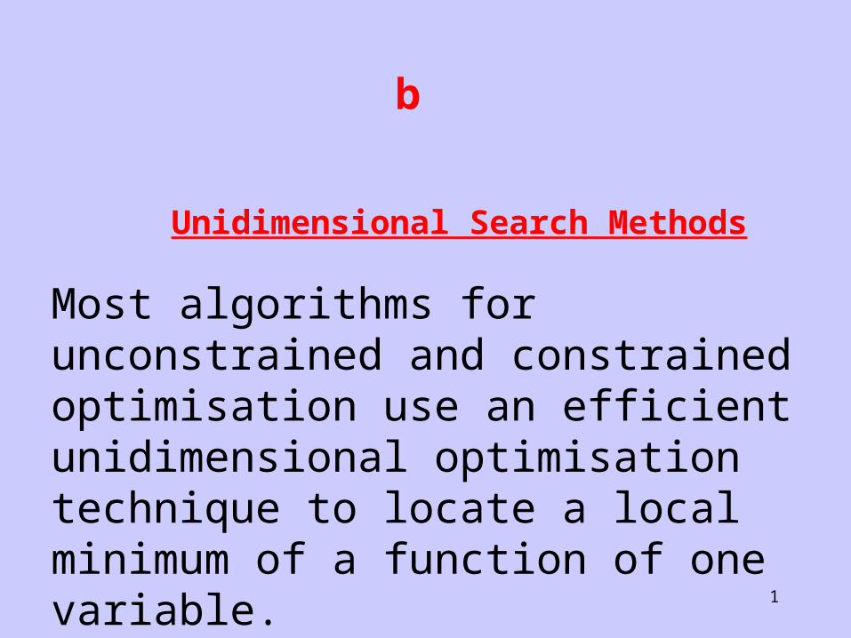
Most algorithms for unconstrained and constrained optimisation use an efficient unidimensional optimisation technique to locate a local minimum of a function of one variable.

2

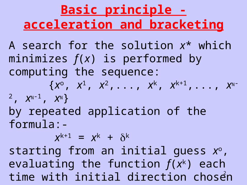
Basic principle - acceleration and bracketing

A search for the solution x* which minimizes f(x) is performed by computing the sequence: {xo, x1, x2,..., xk, xk+1,..., xN-2, xN-1, xN}by repeated application of the formula:- xk+1 = xk + k

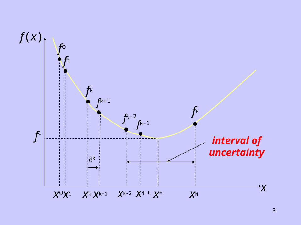
starting from an initial guess xo, evaluating the function f(xk) each time with initial direction chosen such that f(x1) < f(xo), until f(xN) > f(xN-1).

3

x

f(x)

xox1 xkxk+1 xN-1 x* xN

fo

f1

fk

fk+1

fN

fN-2

f*interval ofuncertainty

k

xN-2

fN-1

4

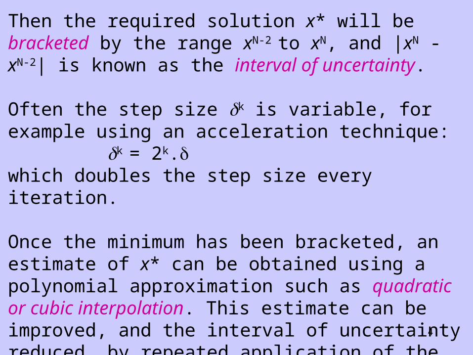
Then the required solution x* will be bracketed by the range xN-2 to xN, and |xN - xN-2| is known as the interval of uncertainty.

Often the step size k is variable, for example using an acceleration technique: k = 2k.which doubles the step size every iteration.

Once the minimum has been bracketed, an estimate of x* can be obtained using a polynomial approximation such as quadratic or cubic interpolation. This estimate can be improved, and the interval of uncertainty reduced, by repeated application of the interpolation.

5

x

f(x)

xN-2 xN-1 xNx* ~*x

fN-2

fN-1

fN

f x hx cx xc

h( ) ~* 1

22

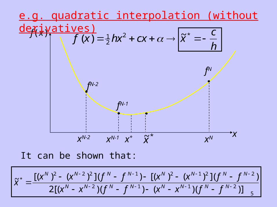
It can be shown that:

~ [( ) ( ) ]( ) [( ) ( ) ]( )

[( )( ) ( )( )]*x

x x f f x x f f

x x f f x x f f

N N N N N N N N

N N N N N N N N

2 2 2 1 2 1 2 2

2 1 1 22

e.g. quadratic interpolation (without derivatives)

6

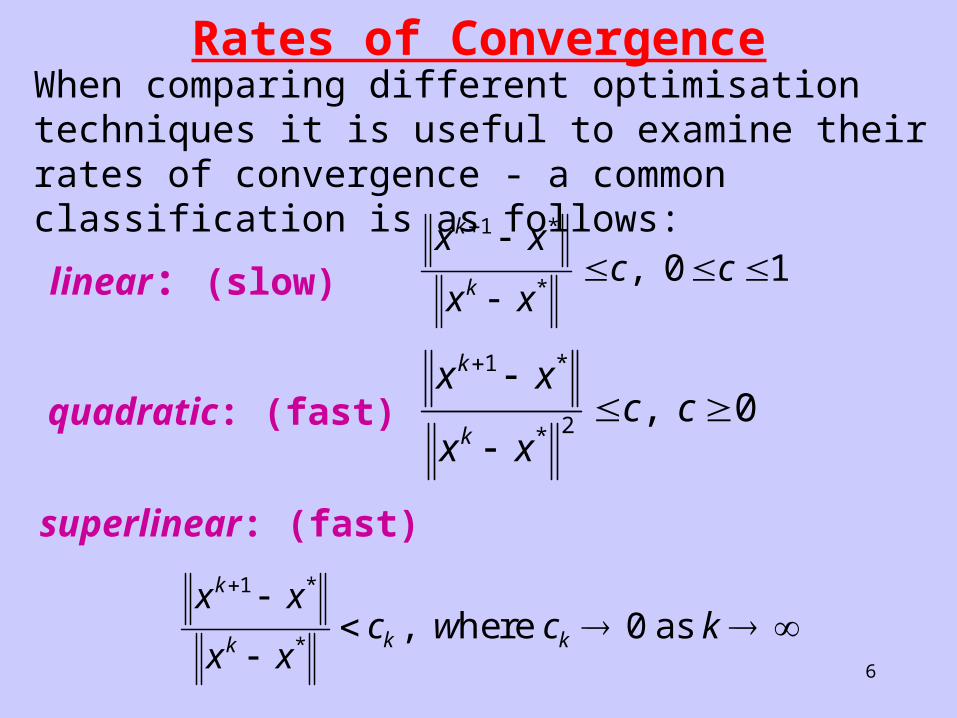
Rates of ConvergenceWhen comparing different optimisation techniques it is useful to examine their rates of convergence - a common classification is as follows: x x

x xc c

k

k

1

0 1*

*,

quadratic: (fast)x x

x xc c

k

k

1

2 0*

*,

superlinear: (fast)

linear: (slow)

x x

x xc w c k

k

k k k

1

0*

*, here as

7

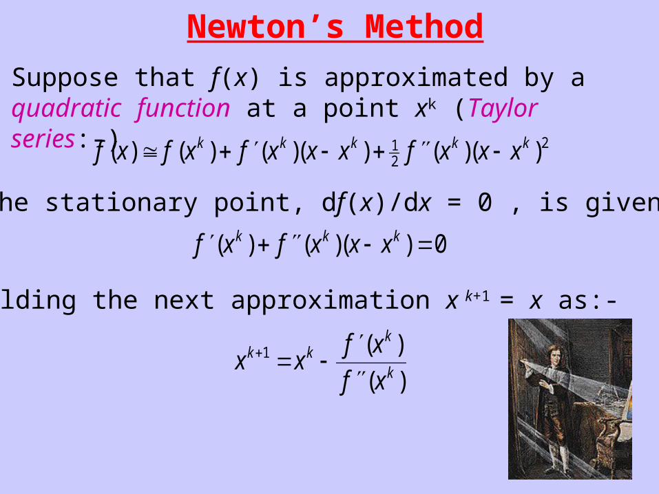
Newton’s Method

Suppose that f(x) is approximated by a quadratic function at a point xk (Taylor series:-)

f x f x f x x x f x x xk k k k k( ) ( ) ( )( ) ( )( ) 12

2

Then the stationary point, df(x)/dx = 0 , is given as:

f x f x x xk k k( ) ( )( ) 0

x xf x

f xk k

k

k

1 ( )

( )

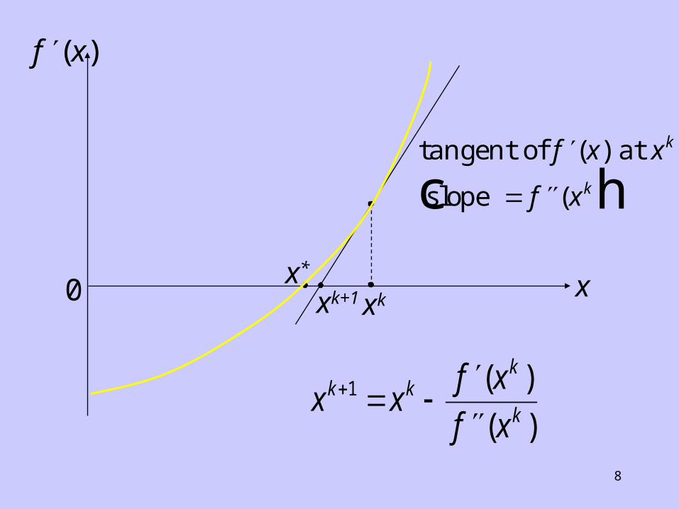
yielding the next approximation x k+1 = x as:-

8

tangent of at

slope

f x x

f x

k

k

( )

(c hx*

xk+1xk x

f x( )

0

x xf x

f xk k

k

k

1 ( )

( )

9

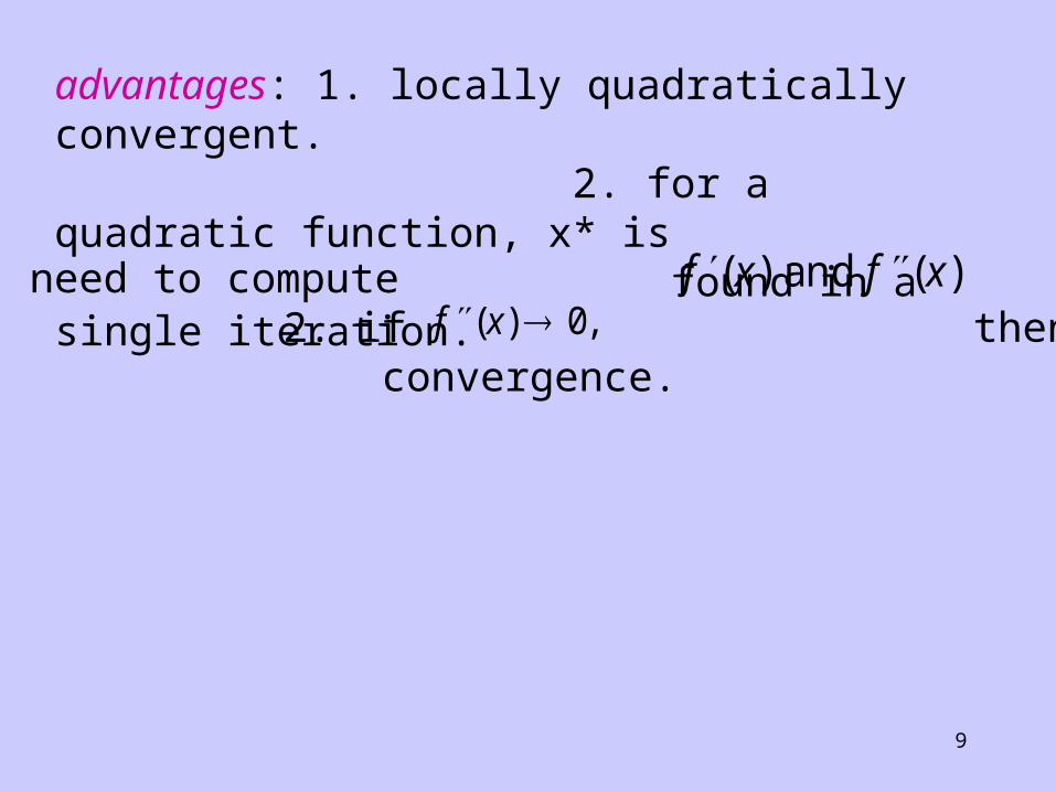
disadvantages: 1. need to compute 2. if then slow convergence.

f x f x( ) ( ) and f x( ) ,0

advantages: 1. locally quadratically convergent. 2. for a quadratic function, x* is found in a single iteration.

10

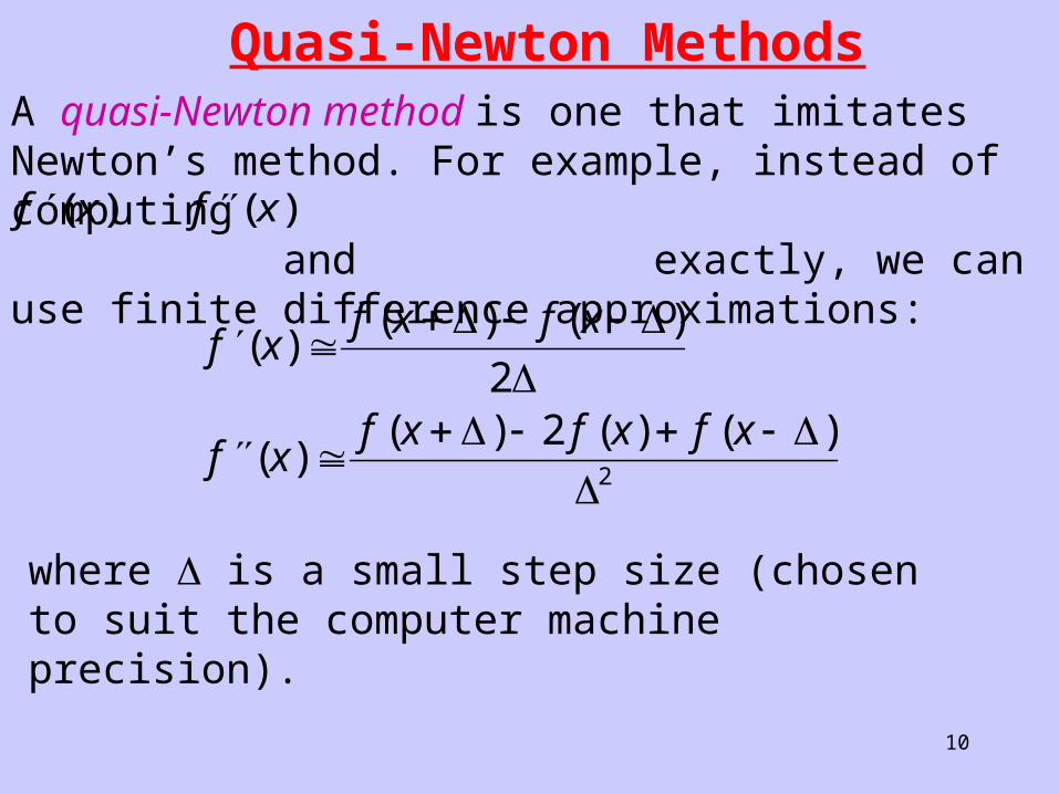
Quasi-Newton MethodsA quasi-Newton method is one that imitates Newton’s method. For example, instead of computing and exactly, we can use finite difference approximations:

f x( ) f x( )

f xf x f x

f xf x f x f x

( )( ) ( )

( )( ) ( ) ( )

22

2

where is a small step size (chosen to suit the computer machine precision).

11

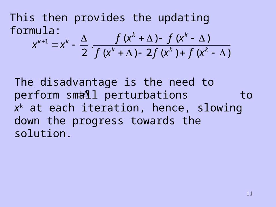
This then provides the updating formula:

x xf x f x

f x f x f xk k

k k

k k k

1

2 2

.( ) ( )

( ) ( ) ( )

The disadvantage is the need to perform small perturbations to xk at each iteration, hence, slowing down the progress towards the solution.

12

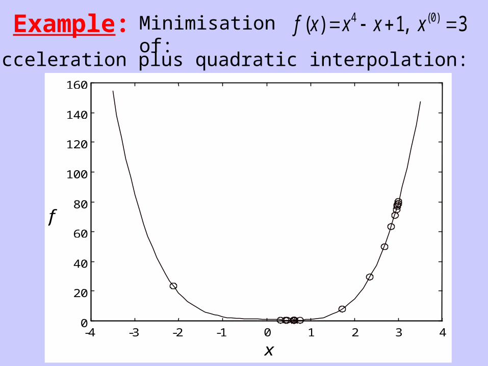
Example:

Minimisation of:

f x x x x( ) , ( ) 4 01 3

(i) acceleration plus quadratic interpolation:

-4 -3 -2 -1 0 1 2 3 4 0

20

40

60

80

100

120

140

160

x

f

13

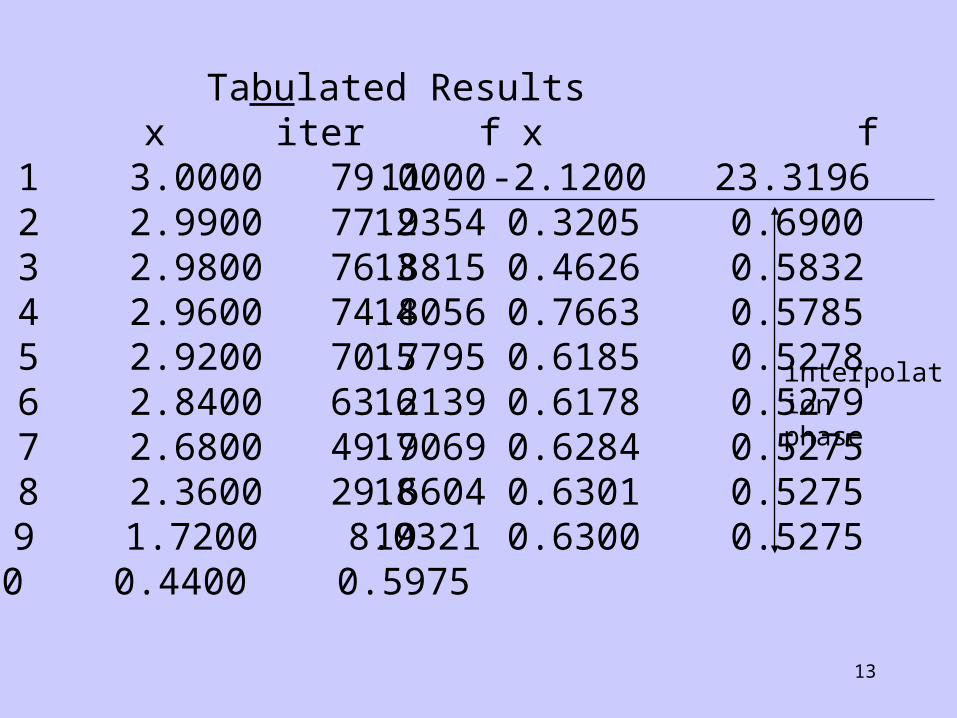
Tabulated Results iter x f 1 3.0000 79.0000 2 2.9900 77.9354 3 2.9800 76.8815 4 2.9600 74.8056 5 2.9200 70.7795 6 2.8400 63.2139 7 2.6800 49.9069 8 2.3600 29.6604 9 1.7200 8.0321 10 0.4400 0.5975

iter x f 11 -2.1200 23.3196 12 0.3205 0.6900 13 0.4626 0.5832 14 0.7663 0.5785 15 0.6185 0.5278 16 0.6178 0.5279 17 0.6284 0.5275 18 0.6301 0.5275 19 0.6300 0.5275

interpolationphase

14

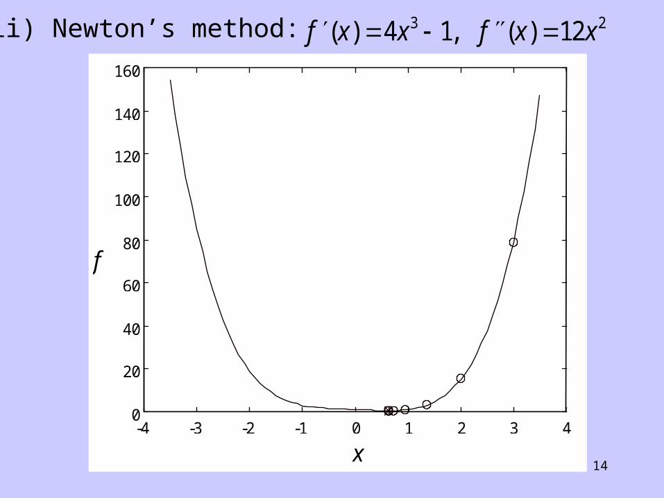
(ii) Newton’s method: f x x f x x( ) , ( )4 1 123 2

-4 -3 -2 -1 0 1 2 3 4 0

20

40

60

80

100

120

140

160

x

f

15

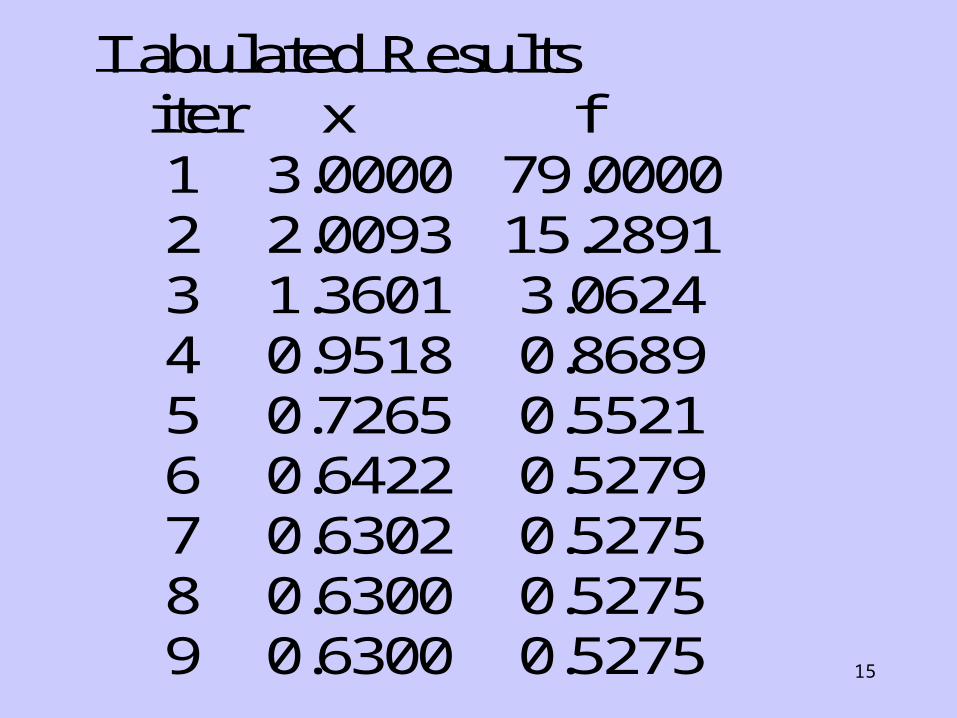
Tabulated Results iter x f 1 3.0000 79.0000 2 2.0093 15.2891 3 1.3601 3.0624 4 0.9518 0.8689 5 0.7265 0.5521 6 0.6422 0.5279 7 0.6302 0.5275 8 0.6300 0.5275 9 0.6300 0.5275

16

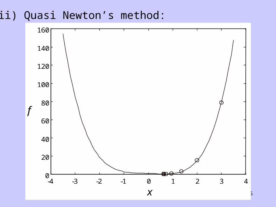
(ii) Quasi Newton’s method:

-4 -3 -2 -1 0 1 2 3 4 0

20

40

60

80

100

120

140

160

x

f

17

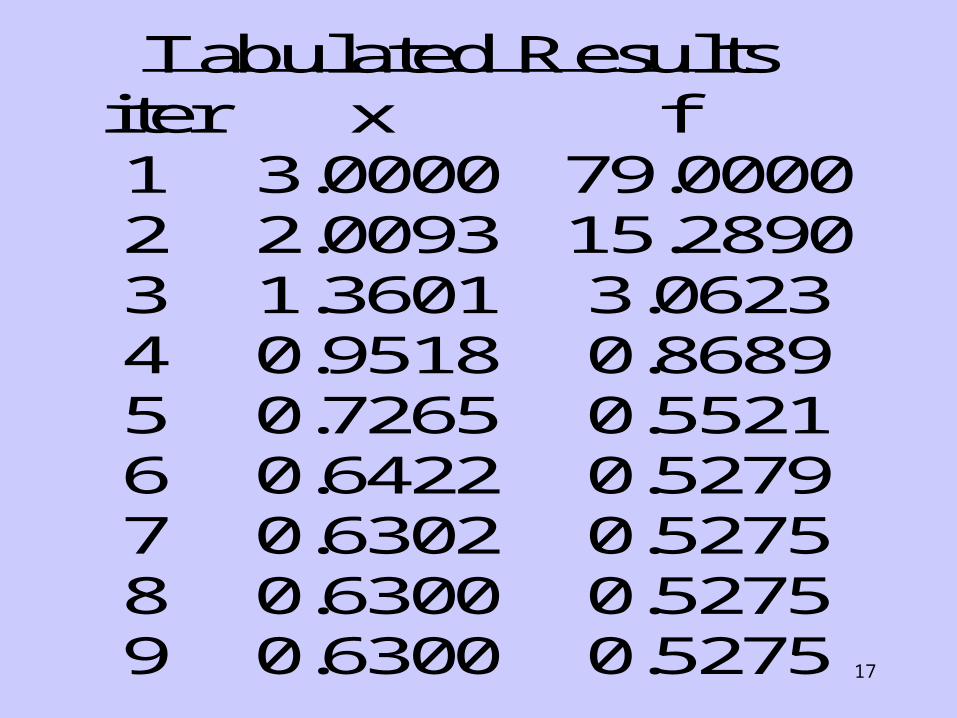
Tabulated Results iter x f 1 3.0000 79.0000 2 2.0093 15.2890 3 1.3601 3.0623 4 0.9518 0.8689 5 0.7265 0.5521 6 0.6422 0.5279 7 0.6302 0.5275 8 0.6300 0.5275 9 0.6300 0.5275

18

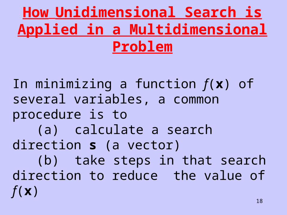
How Unidimensional Search is Applied in a Multidimensional

Problem

In minimizing a function f(x) of several variables, a common procedure is to

(a) calculate a search direction s (a vector)

(b) take steps in that search direction to reduce the value of f(x)

19

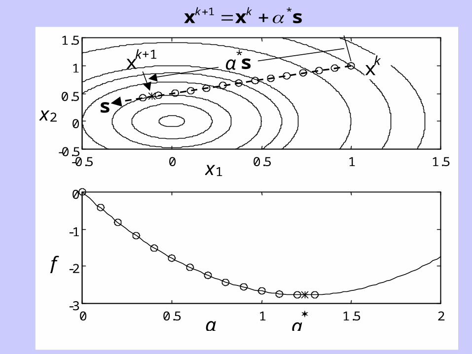
x x sk k 1 *

-0.5 0 0.5 1 1.5 -0.5

0

0.5

1

1.5

x1

x2

0 0.5 1 1.5 2 -3

-2

-1

0

α

f

α

s

xk+1 xk α*s

20

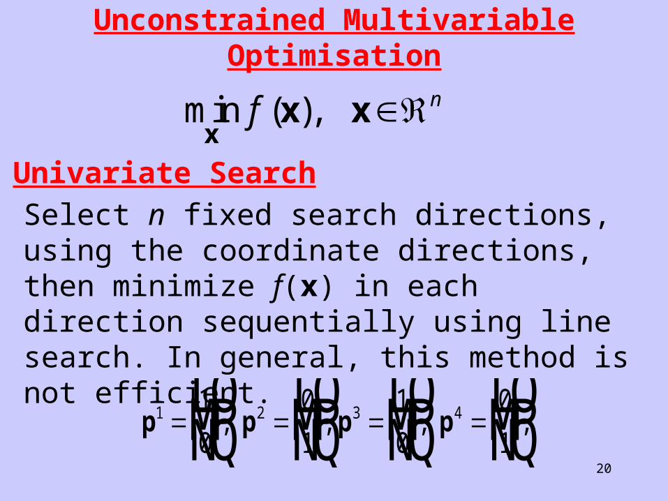
Unconstrained Multivariable Optimisation

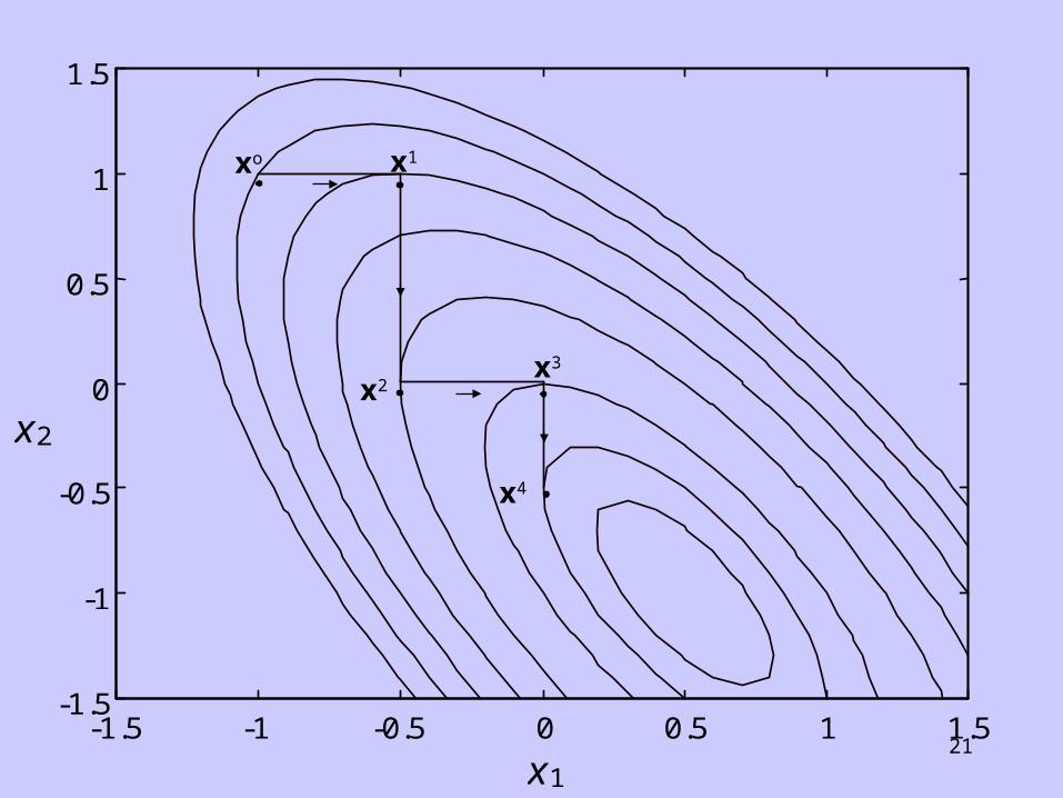
Univariate SearchSelect n fixed search directions, using the coordinate directions, then minimize f(x) in each direction sequentially using line search. In general, this method is not efficient.

min ( ),x

x xf n

p p p p1 2 3 41

0

0

1

1

0

0

1LNMOQP

LNMOQP

LNMOQP

LNMOQP, , , ,

21

-1.5 -1 -0.5 0 0.5 1 1.5 -1.5

-1

-0.5

0

0.5

1

1.5

x1

x2

xo x1

x2x3

x4

22

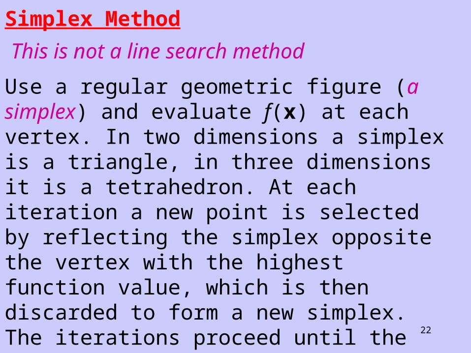
Simplex Method

This is not a line search method

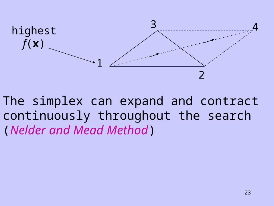
Use a regular geometric figure (a simplex) and evaluate f(x) at each vertex. In two dimensions a simplex is a triangle, in three dimensions it is a tetrahedron. At each iteration a new point is selected by reflecting the simplex opposite the vertex with the highest function value, which is then discarded to form a new simplex. The iterations proceed until the simplex straddles the optimum. The size is reduced and the procedure is repeated.

23

3

12

4highestf(x)

The simplex can expand and contract continuously throughout the search (Nelder and Mead Method)

24

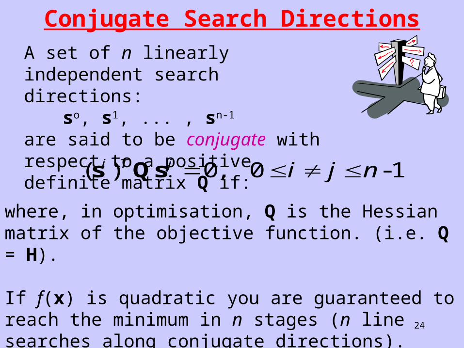
Conjugate Search DirectionsA set of n linearly independent search directions:

so, s1, ... , sn-1

are said to be conjugate with respect to a positive definite matrix Q if: ( ) ,s Qsi T j i j n 0 0 1 -

where, in optimisation, Q is the Hessian matrix of the objective function. (i.e. Q = H).

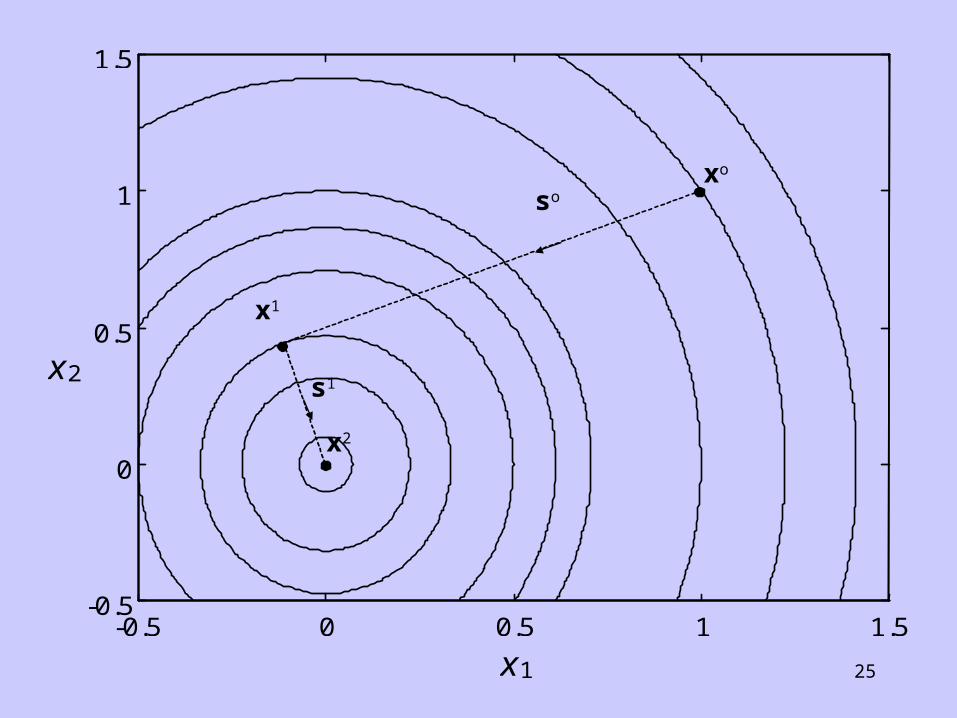
If f(x) is quadratic you are guaranteed to reach the minimum in n stages (n line searches along conjugate directions).

25

-0.5 0 0.5 1 1.5 -0.5

0

0.5

1

1.5

x1

x2

so

s1

xo

x1

x2

26

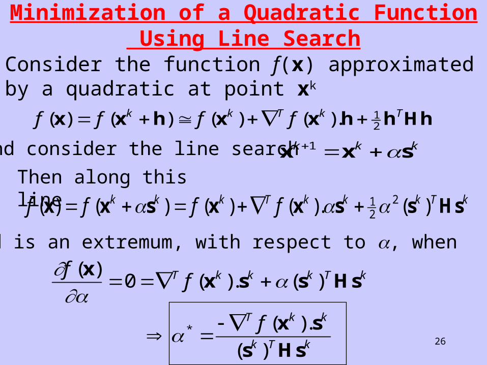
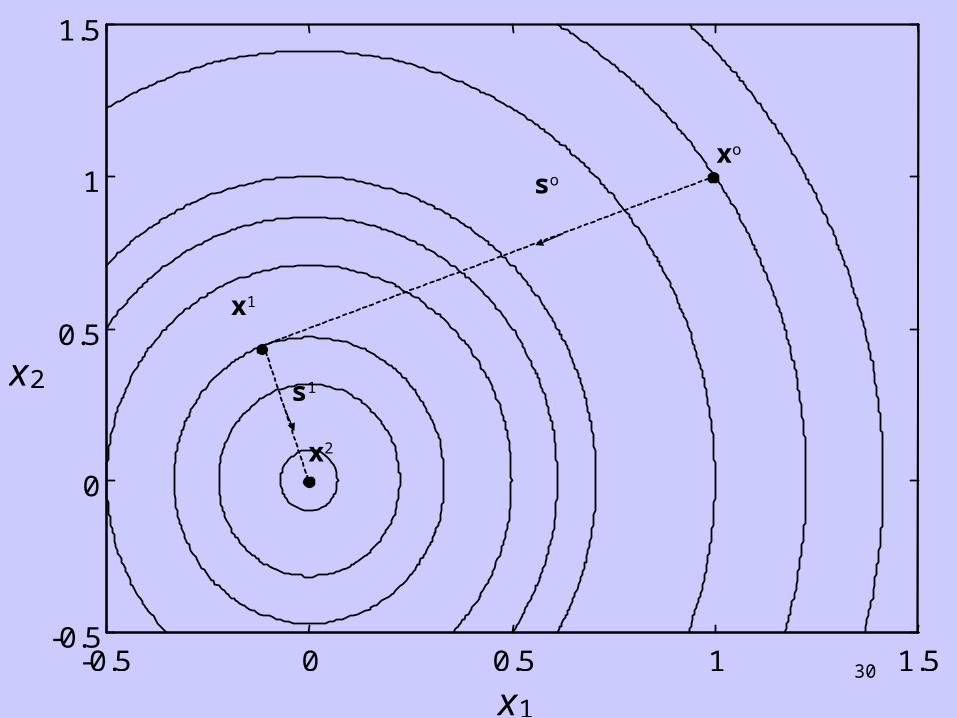
Minimization of a Quadratic Function Using Line Search

Consider the function f(x) approximated by a quadratic at point xk

f f f fk k T k T( ) ( ) ( ) ( ).x x h x x h h Hh 12

and consider the line search x x sk k k 1 Then along this line

f f f fk k k T k k k T k( ) ( ) ( ) ( ). ( )x x s x x s s Hs 12

2

and is an extremum, with respect to , when

ff

f

T k k k T k

T k k

k T k

( )( ). ( )

( ).

( )*

xx s s Hs

x s

s Hs

0

27

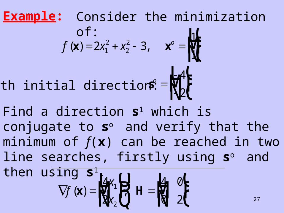
Example: Consider the minimization of:

f x x o( ) ,x x LNMOQP2 3

1

112

22

with initial direction: so LNM

OQP

4

2

Find a direction s1 which is conjugate to so and verify that the minimum of f(x) can be reached in two line searches, firstly using so and then using s1.

LNM

OQP

LNM

OQPf

x

x( ) ,x H

4

2

4 0

0 21

2

28

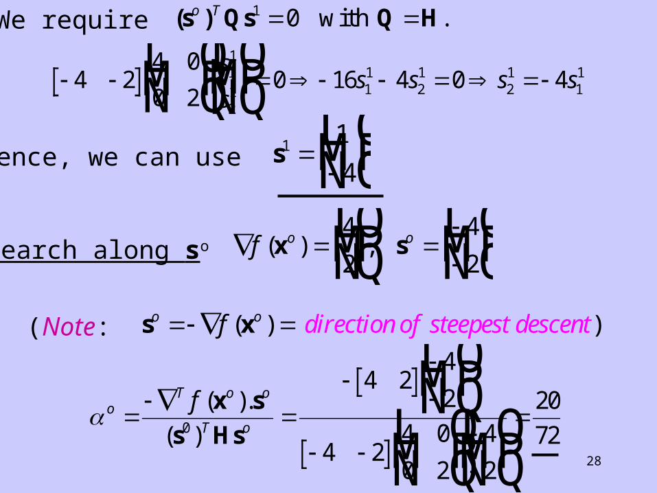
We require (s ) Qs Q Ho T 1 0 with .

LNM

OQPLNMOQP 4 2

4 0

0 20 16 4 0 41

1

21 1

121

21

11s

ss s s s

Hence, we can use s1 1

4

LNM

OQP

Search along so LNMOQP

LNM

OQPf o o( ) ,x s

4

2

4

2

(Note: ( ) )o o direction of steepest descentf s x

oT o o

T o

f

LNM

OQP

LNM

OQP

LNM

OQP

( ).

( )

x s

s Hs0

4 24

2

4 24 0

0 2

4

2

20

72

29

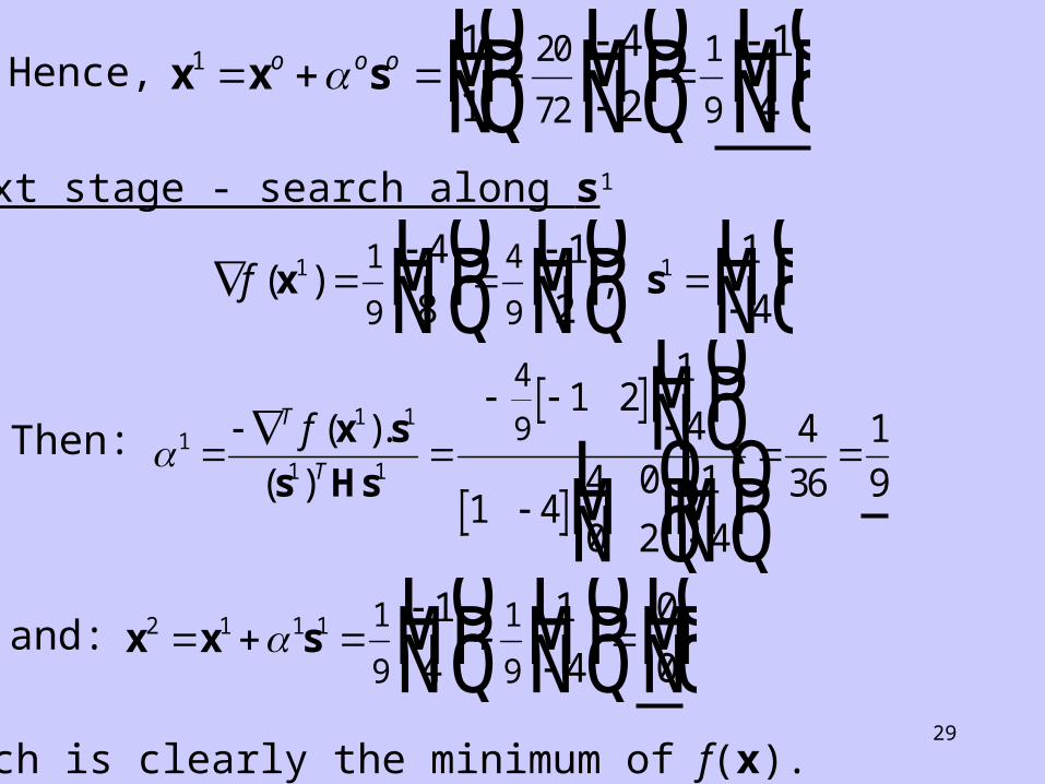
Hence, x x s1 1

1

4

2

1

420

72

1

9

LNMOQP

LNM

OQP

LNM

OQP

o o o

Next stage - search along s1

LNM

OQP

LNM

OQP

LNM

OQPf ( ) ,x s1 11

9

4

9

4

8

1

2

1

4

Then: 11 1

1 1

4

91 2

1

4

1 44 0

0 2

1

4

4

36

1

9

LNM

OQP

LNM

OQPLNM

OQP

T

T

f ( ).

( )

x s

s Hs

and: x x s2 1 1 1 1

9

1

9

1

4

1

4

0

0

LNM

OQP

LNM

OQP

LNMOQP

which is clearly the minimum of f(x).

30

-0.5 0 0.5 1 1.5 -0.5

0

0.5

1

1.5

x1

x2

so

s1

xo

x1

x2

31

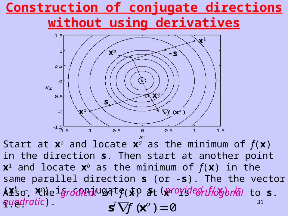
Construction of conjugate directions without using derivatives

-1.5 -1 -0.5 0 0.5 1 1.5 -1.5

-1

-0.5

0

0.5

1

1.5

x1

x2

xo

xa

s

-s

x1

xb

f a( )x

s xT af ( ) 0

Start at xo and locate xa as the minimum of f(x) in the direction s. Then start at another point x1 and locate xb as the minimum of f(x) in the same parallel direction s (or -s). The the vector (xb - xa) is conjugate to s (provided f(x) is quadratic).Also, the gradient of f(x) at xa is orthogonal to s. i.e.

32

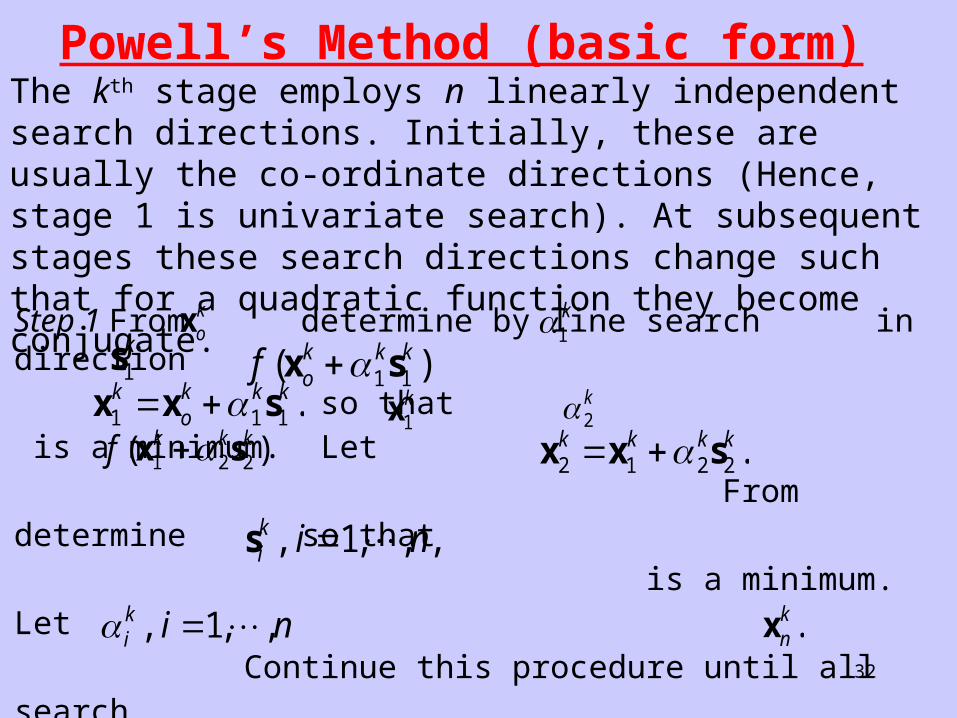
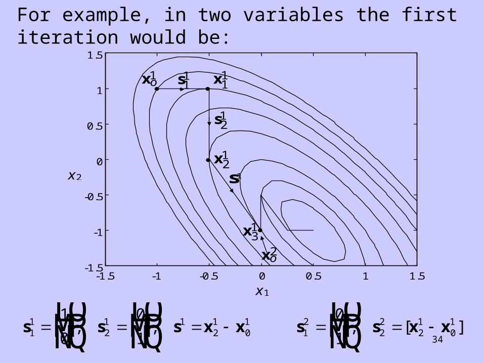
Powell’s Method (basic form) The kth stage employs n linearly independent search directions. Initially, these are usually the co-ordinate directions (Hence, stage 1 is univariate search). At subsequent stages these search directions change such that for a quadratic function they become conjugate. Step 1 From determine by line search in direction so that is a minimum. Let From determine so that is a minimum. Let Continue this procedure until all search directions starting always from the last immediate point in sequence, until all are determined. The final point is

xok

1k

s1k

f ok k k( )x s1 1

x x s1 1 1k

ok k k . x1

k 2k

f k k k( )x s1 2 2 x x s2 1 2 2k k k k .

sik i n, , , , 1

ik i n, , , 1 xn

k .

33

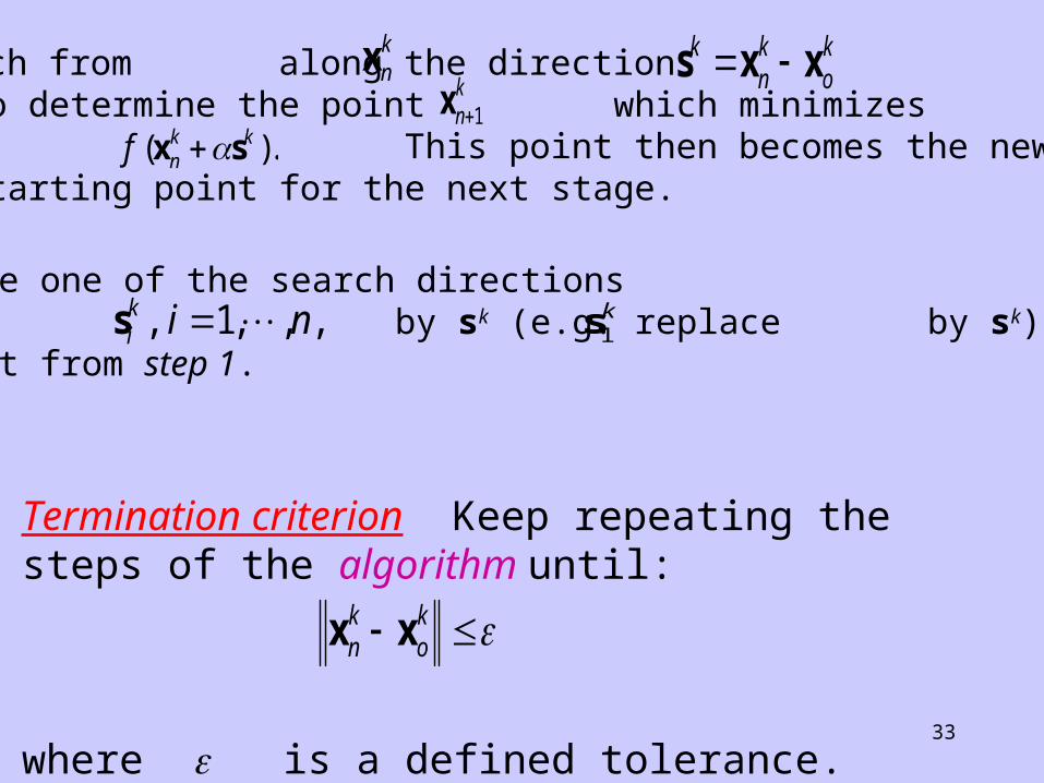
Step 2 Now search from along the direction to determine the point which minimizes This point then becomes the new starting point for the next stage.

f nk k( ).x s

s x xknk

ok

xnk1

xnk

Step 3 Now replace one of the search directions by sk (e.g. replace by sk), and repeat from step 1.

sik i n, , , , 1 s1

k

Termination criterion Keep repeating the steps of the algorithm until:

where is a defined tolerance.

x xnk

ok

34

-1.5 -1 -0.5 0 0.5 1 1.5 -1.5

-1

-0.5

0

0.5

1

1.5

x1

x2

xo1 x1

1

x21

x31

xo2

s11

s21

s1

s s s x x s s x x11

21 1

21

01

12

22

21

011

0

0

1

0

1LNMOQP

LNMOQP

LNMOQP , , , [ ]

For example, in two variables the first iteration would be:

35

Gradient Search Methods

Methods such as univariate, simplex and Powell do not require the use of derivative information in determining the search direction, and are known as direct methods. In general, they are not as efficient as indirect methods which make use of derivatives, first or second, in determining search directions.

For minimization, a good search direction should reduce the objective function at each step of a linear search. i.e.

f fk k( ) ( )x x 1

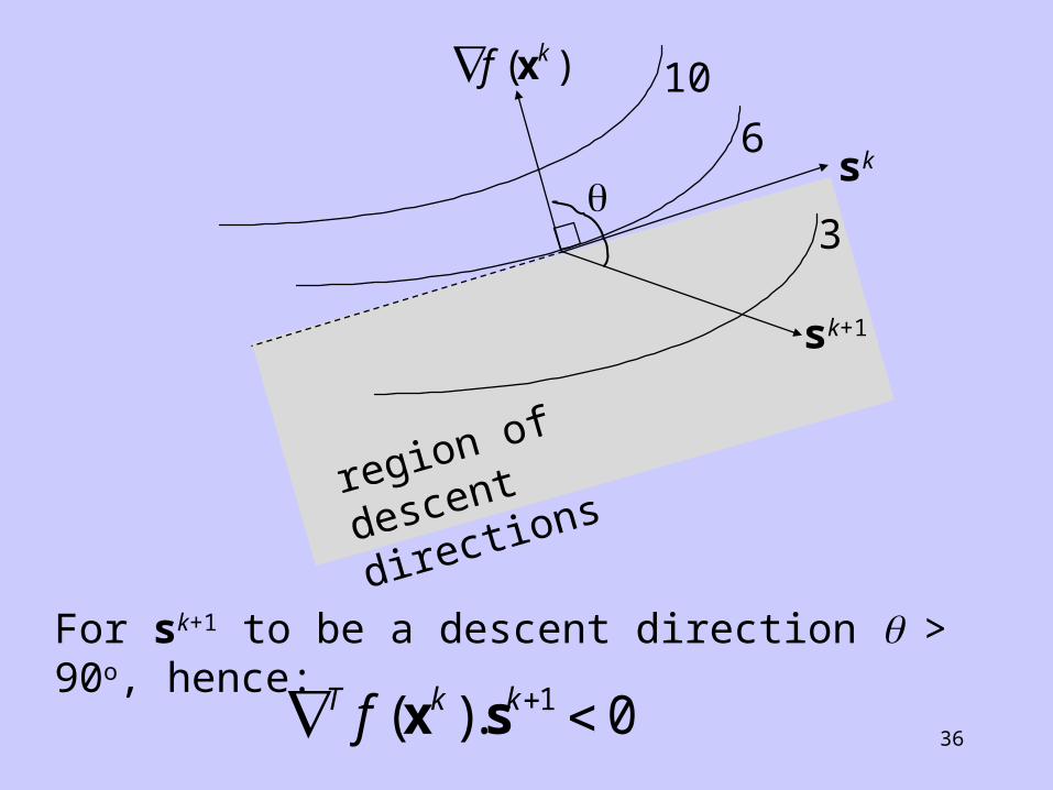
36

For sk+1 to be a descent direction > 90o, hence:

T k kf ( ).x s 1 0

10

6

3

sk

sk+1

f k( )x

region of descent

directions

37

Method of Steepest DescentThe gradient gives the direction of local greatest increase of f(x) and is normal to the contour of f(x) at x. Hence, a local search direction:

f ( )x

s xk kf ( )will give the greatest local decrease of f(x). This is the basis of the steepest descent algorithm.

38

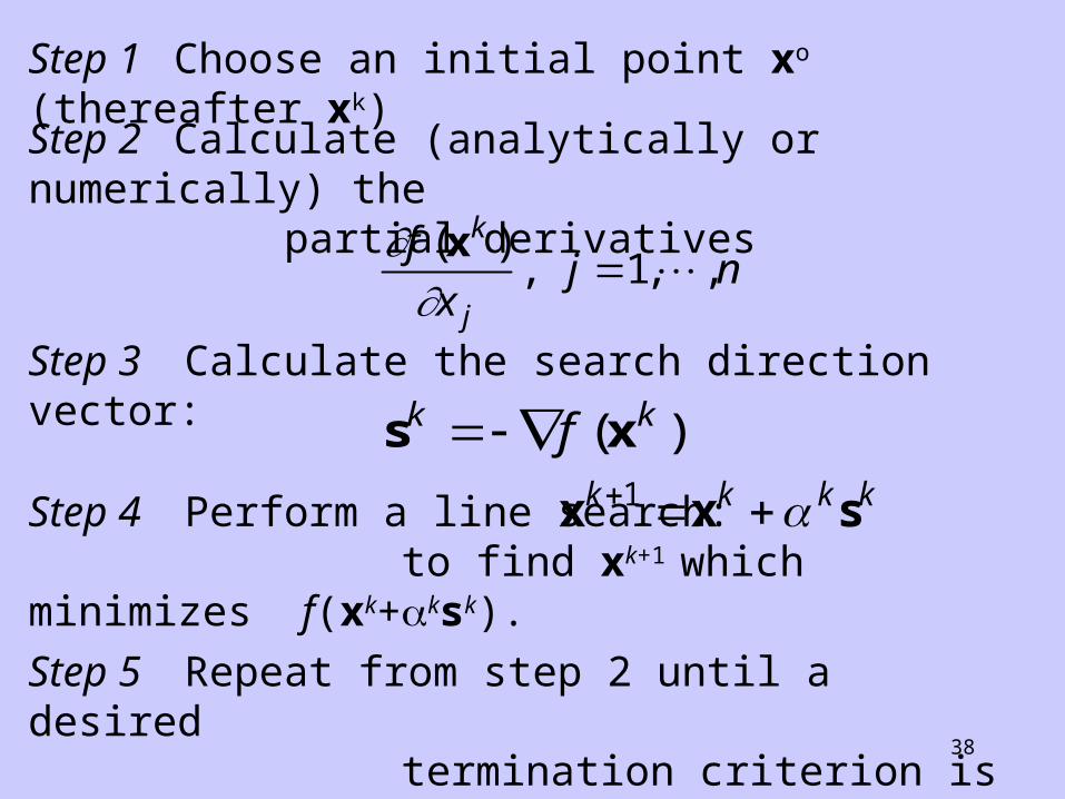
Step 1 Choose an initial point xo (thereafter xk)Step 2 Calculate (analytically or numerically) the

partial derivativesf

xj n

k

j

( ), , ,

x 1

Step 3 Calculate the search direction vector:

s xk kf ( )

Step 4 Perform a line search: to find xk+1 which minimizes f(xk+ksk).

x x sk k k k 1

Step 5 Repeat from step 2 until a desired termination criterion is satisfied.

39

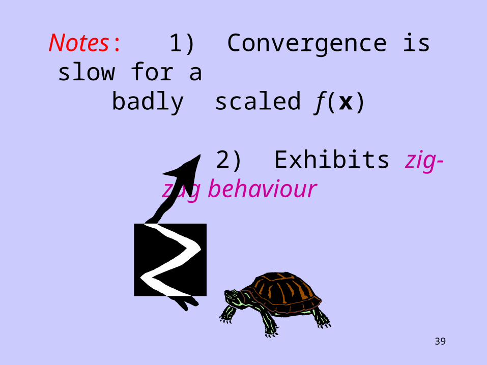
Notes: 1) Convergence is slow for a badly scaled f(x)

2) Exhibits zig-zag behaviour

40

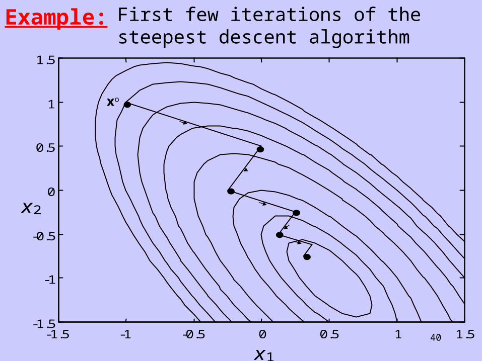
Example:

First few iterations of the steepest descent algorithm

-1.5 -1 -0.5 0 0.5 1 1.5 -1.5

-1

-0.5

0

0.5

1

1.5

x1

x2

xo

41

Fletcher and Reeves Conjugate Gradient Method

This method computes the new search direction by a linear combination of the current gradient and the previous search direction. For a quadratic function this produces conjugate search directions and, hence, will minimize such a function in at most n iterations. The method represents a major improvement over the steepest descent algorithm with only minor extra computational requirements.

42

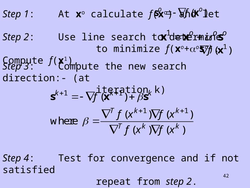
Step 1: At xo calculate f(xo) and let s xo of ( )

Step 2: Use line search to determine to minimize f(xo+oso). Compute f(x1),

x x s1 o o of ( )x1

Step 3: Compute the new search direction:- (at iteration k)

s x sk k k

T k k

T k k

f

f x f x

f x f x

1 1

1 1

( )

( ) ( )

( ) ( )

where

Step 4: Test for convergence and if not satisfied repeat from step 2.

43

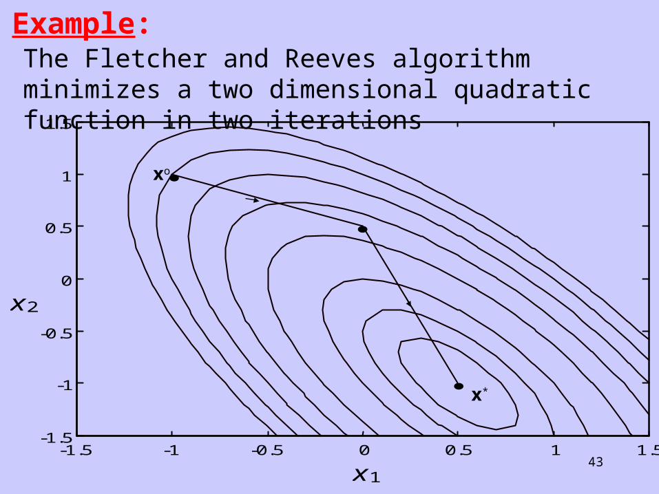
Example:The Fletcher and Reeves algorithm minimizes a two dimensional quadratic function in two iterations

-1.5 -1 -0.5 0 0.5 1 1.5 -1.5

-1

-0.5

0

0.5

1

1.5

x1

x2

x*

xo

44

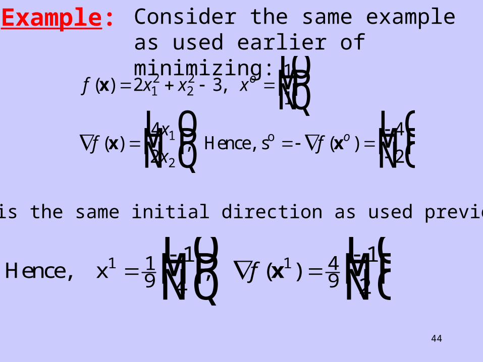
Example: Consider the same example as used earlier of minimizing:

f x x x

fx

xf

o

o

( ) ,

( ) , ( )

x

x x

LNMOQP

LNM

OQP

LNM

OQP

2 31

1

4

2

4

2

12

22

1

2

Hence, so

which is the same initial direction as used previously.

Hence, x 1 LNM

OQP

LNM

OQP

19

49

1

4

1

21, ( )f x

45

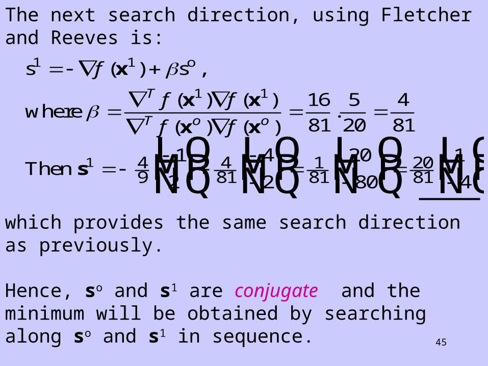
The next search direction, using Fletcher and Reeves is:

s s

where

Then

1 o

LNM

OQP

LNM

OQP

LNM

OQP

LNM

OQP

f

f f

f f

T

T o o

( ) ,

( ) ( )

( ) ( ).

x

x x

x x

s

1

1 1

1

16

81

5

20

4

81

1

2

4

2

20

80

1

449

481

181

2081

which provides the same search direction as previously.

Hence, so and s1 are conjugate and the minimum will be obtained by searching along so and s1 in sequence.

46

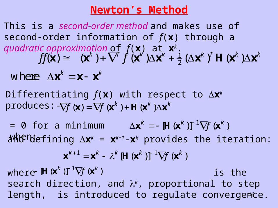
Newton’s MethodThis is a second-order method and makes use of second-order information of f(x) through a quadratic approximation of f(x) at xk.

12 ( ) ( ) ( ) ( ) ( )

where

k T k k k T k k

k k

f f f

x x x x x H x x

x x x

Differentiating f(x) with respect to xk produces:- f f k k k( ) ( ) ( )x x H x x

= 0 for a minimum when:-

x H x xk k kf [ ( )] ( )1

and defining xk = xk+1-xk provides the iteration:

where is the search direction, and k, proportional to step length, is introduced to regulate convergence.

x x H x xk k k k kf 1 1 [ ( )] ( )

[ ( )] ( )H x xk kf1

47

disadvantage: need to determine, analytically or numerically, second order partial derivatives in order to compute the Hessian matrix H(x).

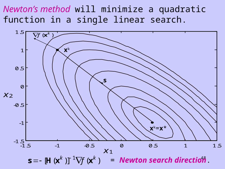
48s H x x [ ( )] ( )k kf1 = Newton search direction.

Newton’s method will minimize a quadratic function in a single linear search.

-1.5 -1 -0.5 0 0.5 1 1.5 -1.5

-1

-0.5

0

0.5

1

1.5

x1

x2

xk=x*

xk

s

f k( )x

49

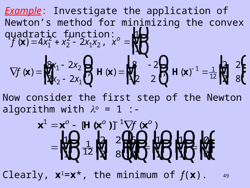
Example: Investigate the application of Newton’s method for minimizing the convex quadratic function:

f x x x x x

fx x

x x

o( ) ,

( ) , ( ) , ( )

x

x H x H x

LNMOQP

LNM

OQP

LNM

OQP

LNM

OQP

4 21

1

8 2

2 2

8 2

2 2

2 2

2 8

12

22

1 2

1 2

2 1

1 112

Now consider the first step of the Newton algorithm with o = 1 :-

x x H(x ) x1 1

1

1

2 2

2 8

6

0

1

1

1

1

0

01

12

LNMOQP

LNM

OQPLNMOQP

LNMOQP

LNMOQP

LNMOQP

o o of[ ] ( )

Clearly, x1=x*, the minimum of f(x).

50

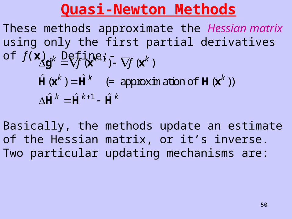
Quasi-Newton MethodsThese methods approximate the Hessian matrix using only the first partial derivatives of f(x). Define:-

g x x

H x H H x

H H H

k k k

k k k

k k k

f f

( ) ( )

( ) ( ))

1

1

(= approximation of

Basically, the methods update an estimate of the Hessian matrix, or it’s inverse. Two particular updating mechanisms are:

51

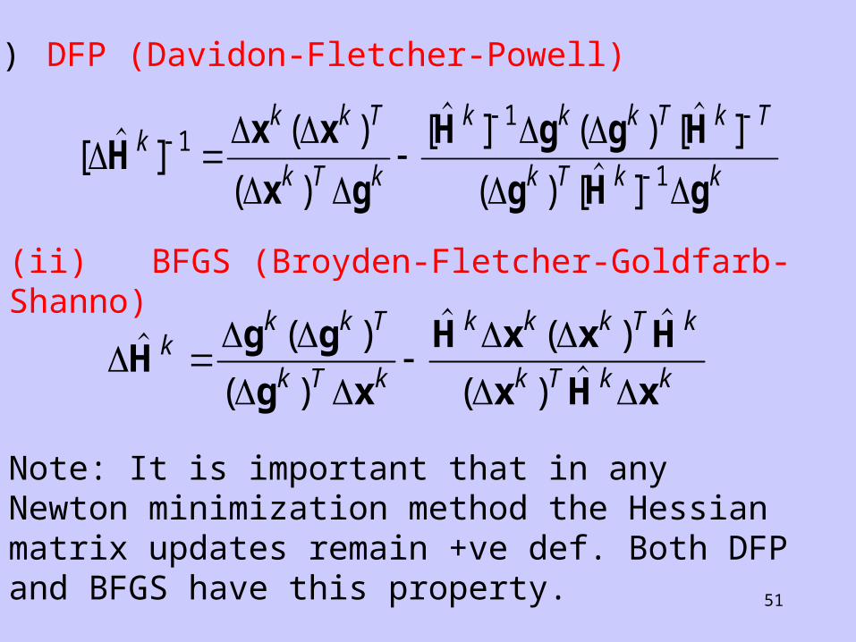
(i) DFP (Davidon-Fletcher-Powell)

[ ]( )

( )

[ ] ( ) [ ]

( ) [ ]

Hx x

x g

H g g H

g H gk

k k T

k T k

k k k T k T

k T k k

11

1

(ii) BFGS (Broyden-Fletcher-Goldfarb-Shanno)

( )

( )

( )

( ) Hg g

g x

H x x H

x H xk

k k T

k T k

k k k T k

k T k k

Note: It is important that in any Newton minimization method the Hessian matrix updates remain +ve def. Both DFP and BFGS have this property.

52

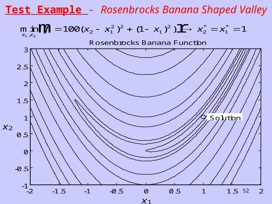
Test Example - Rosenbrocks Banana Shaped Valley

min ( ) ( ) ),

* *

x xf x x x x x

1 2

100 1 12 12 2

12

2 1 m r

-2 -1.5 -1 -0.5 0 0.5 1 1.5 2 -1

-0.5

0

0.5

1

1.5

2

2.5

3 Rosenbrocks Banana Function

x1

x2 Solution

53

It is called the banana function because of the way the curvature bends around the origin. It is notorious in optimization examples because of the slow convergence with which most methods exhibit when trying to solve this problem.

54

55

-2 -1.5 -1 -0.5 0 0.5 1 1.5 2-1

-0.5

0

0.5

1

1.5

2

2.5

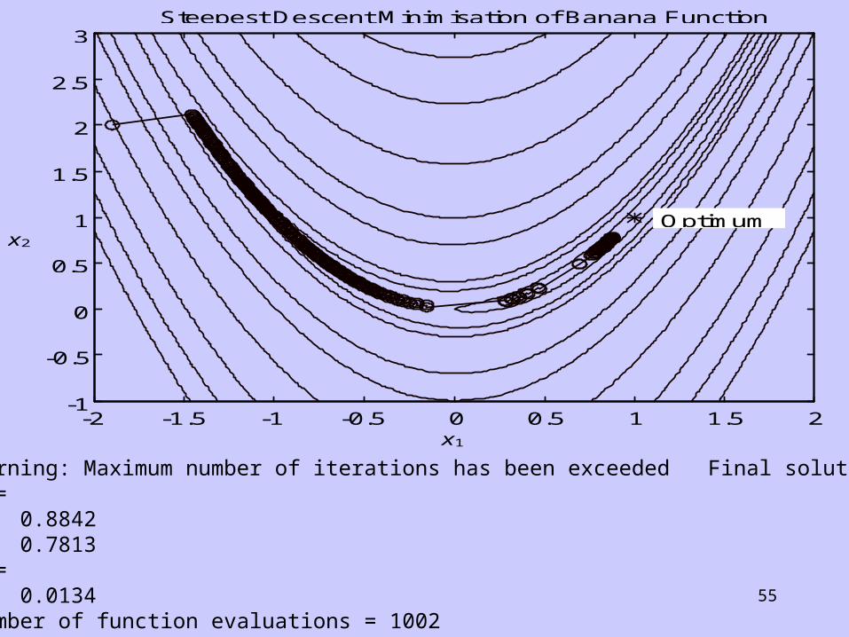
3Steepest Descent Minimisation of Banana Function

x1

x2

Optimum

Warning: Maximum number of iterations has been exceeded Final solution:x = 0.8842 0.7813f = 0.0134number of function evaluations = 1002

56

-2 -1.5 -1 -0.5 0 0.5 1 1.5 2-1

-0.5

0

0.5

1

1.5

2

2.5

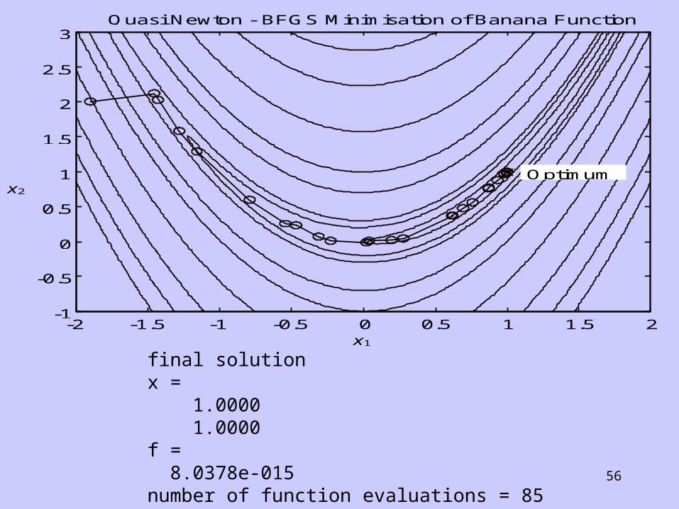
3Quasi Newton - BFGS Minimisation of Banana Function

x1

x2

Optimum

final solutionx = 1.0000 1.0000f = 8.0378e-015number of function evaluations = 85

57

-2 -1.5 -1 -0.5 0 0.5 1 1.5 2-1

-0.5

0

0.5

1

1.5

2

2.5

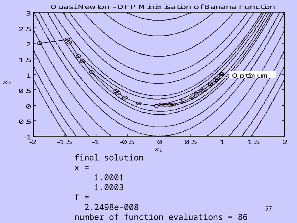
3Quasi Newton - DFP Minimisation of Banana Function

x1

x2

Optimum

final solutionx = 1.0001 1.0003f = 2.2498e-008number of function evaluations = 86

58

-2 -1.5 -1 -0.5 0 0.5 1 1.5 2-1

-0.5

0

0.5

1

1.5

2

2.5

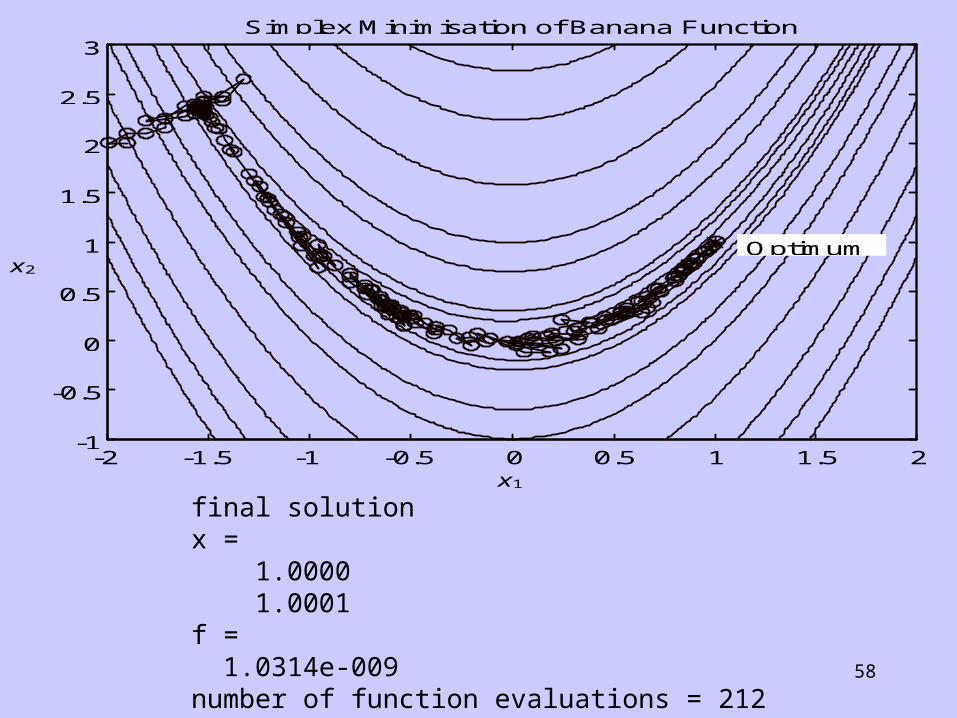
3Simplex Minimisation of Banana Function

x1

x2

Optimum

final solutionx = 1.0000 1.0001f = 1.0314e-009number of function evaluations = 212

59

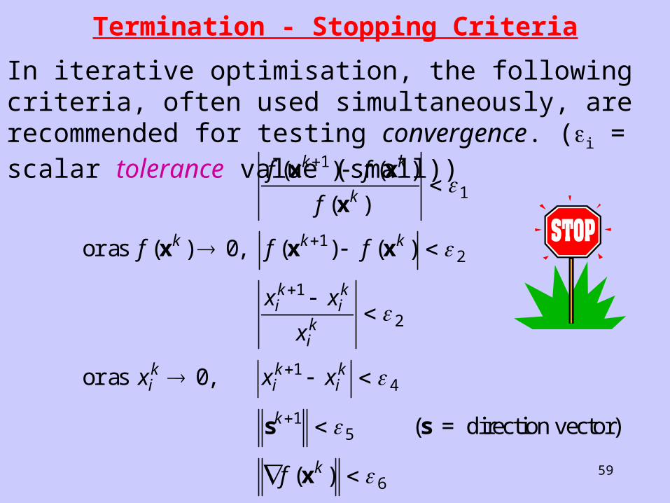
Termination - Stopping Criteria

In iterative optimisation, the following criteria, often used simultaneously, are recommended for testing convergence. (i = scalar tolerance value (small))

or as

or as

( = direction vector)

f f

f

f f f

x x

x

x x x

f

k k

k

k k k

ik

ik

ik

ik

ik

ik

k

k

( ) ( )

( )

( ) , ( ) ( )

,

( )

x x

x

x x x

s s

x

1

1

12

1

2

14

15

6

0

0

60

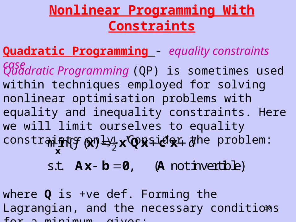
Nonlinear Programming With Constraints

Quadratic Programming - equality constraints caseQuadratic Programming (QP) is sometimes used within techniques employed for solving nonlinear optimisation problems with equality and inequality constraints. Here we will limit ourselves to equality constraints only. Consider the problem: 1

2min{ ( )

s.t. , ( not invertible)

T Tf d

x

x x Qx c x

Ax b 0 A

where Q is +ve def. Forming the Lagrangian, and the necessary conditions for a minimum, gives:

61

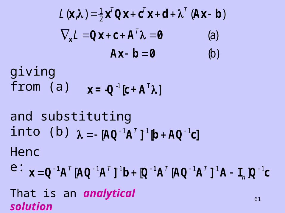
12( , ) ( ) T T TL x x Qx c x d Ax b

That is an analytical solution

(a)

(b)

TL

x Qx c A 0

Ax b 0

1 T ]-x = -Q [c + A giving from (a)

1 1 1 [ T AQ A ] [b AQ c]and substituting into (b)

1 1 1 1 1 [ [ [ ]T T T Tn

1 1x Q A AQ A ] b Q A AQ A ] A I Q c

Hence:

62

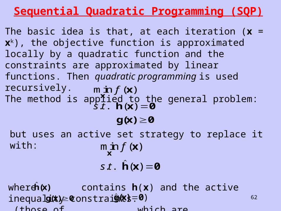
Sequential Quadratic Programming (SQP)

The basic idea is that, at each iteration (x = xk), the objective function is approximated locally by a quadratic function and the constraints are approximated by linear functions. Then quadratic programming is used recursively.The method is applied to the general problem:min ( )

. . ( )x

x

h x 0

g(x) 0

f

s t

but uses an active set strategy to replace it with:min ( )

. . ( )

xx

h x 0

f

s t

where contains h(x) and the active inequality constraints. (those of which are

h(x)g(x) 0 )g(x) 0

63

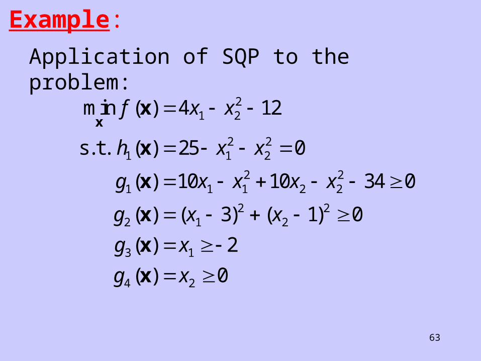
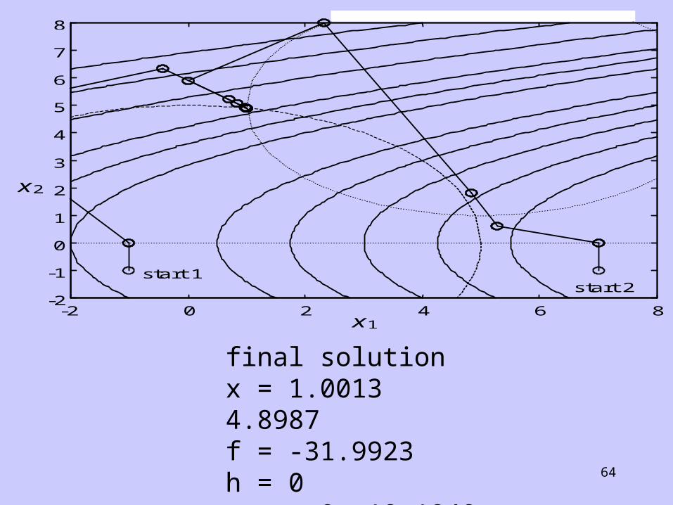
Example:

min ( )

( )

( )

( ) ( ) ( )

( )

( )

xx

x

x

x

x

x

f x x

h x x

g x x x x

g x x

g x

g x

4 12

25 0

10 10 34 0

3 1 0

2

0

1 22

1 12

22

1 1 12

2 22

2 12

22

3 1

4 2

s.t.

Application of SQP to the problem:

64

-2 0 2 4 6 8 -2

-1

0

1

2

3

4

5

6

7

8

x1

x2

start 1 start 2

final solutionx = 1.0013 4.8987f = -31.9923h = 0g = 0 19.1949

65

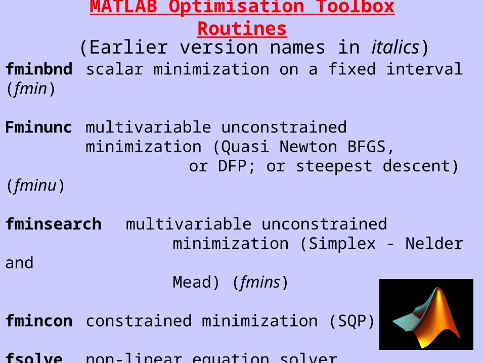
MATLAB Optimisation Toolbox Routines

fminbnd scalar minimization on a fixed interval (fmin)

Fminunc multivariable unconstrainedminimization (Quasi Newton BFGS,

or DFP; or steepest descent) (fminu)

fminsearch multivariable unconstrained minimization (Simplex - Nelder and Mead) (fmins)

fmincon constrained minimization (SQP) (constr)

fsolve non-linear equation solver

linprog linear programming (lp)

(Earlier version names in italics)

66

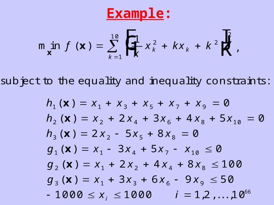
Example:

m in ( )x

xfk

x k x kk kk

FHG

IKJ

1 2 2

1

1 0 2

,

su b je c t to the e q u a lity a nd ine q u a lity c o nst ra in ts :

h x x x x x

h x x x x x

h x x x

g x x x x

g x x x x

g x x x x

x ii

1 1 3 5 7 9

2 2 4 6 8 1 0

3 2 5 8

1 1 4 7 1 0

2 1 2 4 8

3 1 3 6 9

0

2 3 4 5 0

2 5 8 0

3 5 0

2 4 8 1 0 0

3 6 9 5 0

1 0 0 0 1 0 0 0 1 2 1 0

( )

( )

( )

( )

( )

( )

, , . . . ,

x

x

x

x

x

x

67

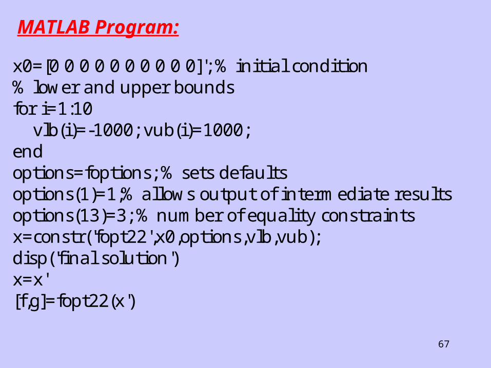
x0=[0 0 0 0 0 0 0 0 0 0]'; % initial condition% lower and upper boundsfor i=1:10 vlb(i)=-1000; vub(i)=1000;endoptions=foptions; % sets defaultsoptions(1)=1;% allows output of intermediate resultsoptions(13)=3; % number of equality constraintsx=constr('fopt22',x0,options,vlb,vub);disp('final solution')x=x'[f,g]=fopt22(x')

MATLAB Program:

68

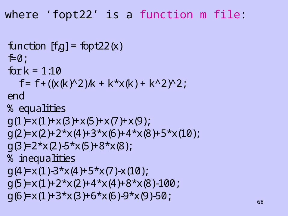
function [f,g] = fopt22(x)f=0;for k = 1:10 f = f +((x(k) 2̂)/k + k*x(k) + k 2̂) 2̂;end% equalitiesg(1)=x(1)+x(3)+x(5)+x(7)+x(9);g(2)=x(2)+2*x(4)+3*x(6)+4*x(8)+5*x(10);g(3)=2*x(2)-5*x(5)+8*x(8);% inequalitiesg(4)=x(1)-3*x(4)+5*x(7)-x(10);g(5)=x(1)+2*x(2)+4*x(4)+8*x(8)-100;g(6)=x(1)+3*x(3)+6*x(6)-9*x(9)-50;

where ‘fopt22’ is a function m file:

69

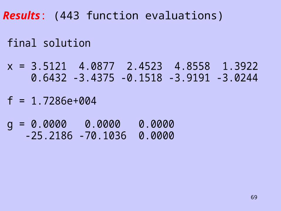
final solution

x = 3.5121 4.0877 2.4523 4.8558 1.3922 0.6432 -3.4375 -0.1518 -3.9191 -3.0244

f = 1.7286e+004

g = 0.0000 0.0000 0.0000 -25.2186 -70.1036 0.0000

Results: (443 function evaluations)