Embed Size (px)
Citation preview
FINITE ELEMENT ANALYSIS AND EXPERIMENTAL VALIDATION OF REINFORCED
CONCRETE SINGLE-MAT SLABS SUBJECTED TO BLAST LOADS
A THESIS IN
Civil Engineering
Submitted to the Faculty of the University of
Missouri-Kansas City in partial fulfillment of
requirements for the degree of
MASTER OF SCIENCE
by
Akash Ashok Iwalekar
Bachelor of Civil Engineering (B.E.)
University of Mumbai – G. V. Acharya Institution of Technology
University of Missouri-Kansas City
2018

2018
Akash Ashok Iwalekar
All Rights Received.
iii
FINITE ELEMENT ANALYSIS AND EXPERIMENTAL VALIDATION OF REINFORCED
CONCRETE SINGLE-MAT SLABS SUBJECTED TO BLAST LOADS
Akash Ashok Iwalekar, Candidate for the Master of Science Degree,
University of Missouri- Kansas City
ABSTRACT
The study carried out in this thesis is the investigation of the behavior of
reinforced concrete slabs subjected to blast loading. A separate experimental study was performed
involving twelve reinforced concrete (RC) slabs in a shock tube (Blast Load Simulator). Records
from this experimental study were used for performing finite element analysis. Numerical
simulation done in this research investigated the effect of using various bond-slip models in
studying the behavior of these twelve RC slabs subjected to blast loading.
LS-DYNA®, a non-linear transient dynamic finite element analysis program,
was used in this study. Finite element models for twelve slabs using the LS-DYNA® subjected to
experimental blast loads were used to study the bond-slip behavior between steel reinforcing bars
and concrete. High-strength concrete reinforced with high-strength steel slabs and normal-strength
concrete reinforced with normal-strength steel slabs were the two material combinations used in
this research. The primary objective of this study was the investigation of two bond interaction
system between steel and concrete, available in LS-DYNA®, for the two material combinations
under blast loading. The assumption of a perfect-bond between concrete and steel was the first
bond interaction system studied, utilizing Constrained Lagrange in Solid Formulation. Beam bond
iv
is another bond interaction system investigated using Beam in Solid formulation in the program.
Furthermore, three functions were investigated in the beam bond interaction system along with the
program generated beam bond function. Validation of these interaction systems, with experimental
data, was the goal of the project.
Upon investigation of this research, comparison between results of the finite
element analysis and the experimental validation of reinforced concrete single-mat slabs which
were subjected to blast loading, assisted in the conclusion that the beam bond function proposed
by Murcia-Delso Juan is the most consistent among all of the interaction systems. However, with
slight modifications in the beam bond function proposed by Grassl, which is identical to the CEB-
FIP model, gives the most accurate results for high strength materials in terms of peak deflection
and residual deflection history. Most accurate prediction to experimental records in given by
perfect bond formulation, and bond-slip fails to give accurate results for blast loading.
v
APPROVAL PAGE
The faculty listed below, appointed by the Dean of the School of Computing and Engineering, has
examined the thesis titled “Finite Element Analysis and Experimental Validation of Reinforced
Concrete Single-Mat Slabs Subjected to Blast Loads,” presented by Akash Ashok Iwalekar,
candidate for Master of Science in Civil Engineering, and certify, that in their opinion, it is worthy
of acceptance.
Supervisory Committee
Thiagarajan Ganesh, Ph.D., P.E., Committee Chair
Department of Civil and Mechanical Engineering
Ceki Halmen, Ph.D., P.E.
Department of Civil and Mechanical Engineering
ZhiQiang Chen, Ph.D.
Department of Civil and Mechanical Engineering
vi
TABLE OF CONTENTS
ABSTRACT……………………………………………………………………………………...iii
LIST OF ILLUSTRATIONS ......................................................................................................... ix
LIST OF TABLES……………………………………………………………………………….xv
CHAPTER 1. INTRODUCTION ................................................................................................... 1
1.1 An overview on Blast Effects on Structures .................................................................... 1
1.2 Significance of Studying Blast Effects on Reinforced Concrete Slabs ............................ 2
1.3 Proposed Solution ............................................................................................................ 3
1.4 Thesis Organization.......................................................................................................... 4
CHAPTER 2. LITERATURE SURVEY ........................................................................................ 6
CHAPTER 3. OBJECTIVE AND SCOPE ................................................................................... 11
3.1 Problem Statement ......................................................................................................... 11
3.2 Objectives ....................................................................................................................... 11
3.3 Tasks............................................................................................................................... 12
CHAPTER 4. EXPERIMENTAL INVESTIGATION ................................................................. 15
4.1 Materials ......................................................................................................................... 16
4.2 Methods .......................................................................................................................... 18
4.3 Experimental Data .......................................................................................................... 19
CHAPTER 5. NUMERICAL MODELING IN LS-DYNA®....................................................... 20
5.1 Significance of Numerical Modeling in LS-DYNA® ................................................... 20
5.2 Geometric Models .......................................................................................................... 21
5.2.1 Meshing for Concrete Model .................................................................................. 21
5.2.2 Meshing for Steel Model ........................................................................................ 23
5.2.3 Hourglass Control in LS-DYNA® ......................................................................... 25
5.2.4 The Constrained Lagrange in Solid formulation .................................................... 26
vii
5.2.5 The Constrained Beam in Solid formulation .......................................................... 26
5.3 Boundary Conditions...................................................................................................... 30
5.4 Material Models in LS-DYNA® .................................................................................... 31
5.4.1 The Concrete Damage Model Release 3 ................................................................. 32
5.4.2 The Plastic Kinematic Model for Steel ................................................................... 36
5.5 Blast Load Application in LS-DYNA® ......................................................................... 36
CHAPTER 6. NUMERICAL ANALUSIS RESULTS AND COMAPRISON WITH
EXPERIMENTAL……………………………………………………………………………….38
6.1 Study NCOUP Parameter of Beam in Solid Formulation .............................................. 39
6.1.1 NCOUP parametric study with JUAN function ..................................................... 39
6.1.2 NCOUP parametric study with CIB-FIP function .................................................. 42
6.1.3 NCOUP parametric study with CIB-FIP-S3 function ............................................ 46
6.2 High Strength Concrete with High Strength Steel Slabs (HSC-V) ................................ 49
6.2.1 Mesh size effect on Slab # 1 (HSC-V1-4in.) .......................................................... 50
6.2.2 Mesh size effect on Slab # 3 (HSC-V2-4in.) .......................................................... 52
6.2.3 Mesh size effect on Slab # 5 (HSC-V3-4in.) .......................................................... 54
6.2.4 Mesh size effect on Slab # 7 (HSC-V4-8in.) .......................................................... 56
6.2.5 Mesh size effect on Slab # 9 (HSC-V5-8in.) .......................................................... 58
6.2.6 Mesh Size Effect for Slab # 11 (HSC-V6-8in.) ...................................................... 61
6.3 Normal Strength Concrete with Normal Strength Steel Slabs (RSC-R) ........................ 62
6.3.1 Mesh size effect on Slab # 2 (RSC-R1-4in.) .......................................................... 63
6.3.2 Mesh Size Effect for Slab # 4 (RSC-R2-4in.) ........................................................ 65
6.3.3 Mesh Size Effect for Slab # 6 (RSC-R3-4in.) ........................................................ 67
6.3.4 Mesh Size Effect for Slab # 8 (RSC-R4-8in.) ........................................................ 70
6.3.5 Mesh Size Effect for Slab # 10 (RSC-R5-8in.) ...................................................... 72
viii
6.3.6 Mesh Size Effect for Slab # 12 (RSC-R6-8in.) ...................................................... 74
CHAPTER 7. DISCUSSION OF RESULTS ............................................................................... 77
7.1 High-Strength Concrete – Comparison of Model with 1 in. (25.4 mm.) Mesh to ½ in.
(12.7 mm.) Mesh Model. ........................................................................................................... 77
7.2 Normal-Strength Concrete – Comparison of Model with 1 in. (25.4 mm.) Mesh to ½ in.
(12.7 mm.) Mesh Model. ........................................................................................................... 79
7.3 Mesh Size Effects ........................................................................................................... 82
CHAPTER 8. CONCLUSION AND FUTURE WORK .............................................................. 84
8.1 Future Scope of Work .................................................................................................... 85
APPENDIX A - PRESSURE AND IMPULSE DATA FOR 12 SLABS ..................................... 86
APPENDIX B - PRESSURE AND IMPULSE PLOTS FOR 12 RC SLABS ............................. 87
APPENDIX C - SUMMARY TABLES ....................................................................................... 93
APPENDIX D – LS-DYNA INPUT............................................................................................. 95
REFERENCES…………………………………………………………………………………107
VITA……………………………………………………………………………………………111
ix
LIST OF ILLUSTRATIONS
Figure 4.1-1: Single-mat reinforced concrete (rc) slab with 4 in. Type single layer reinforcement
........................................................................................................................................... 17
Figure 4.1-2: Single-mat reinforced concrete (rc) slab with 8 in. Type single layer reinforcement
........................................................................................................................................... 17
Figure 4.2-1: Blas load simulator (shock tube) ............................................................................. 18
Figure 5.3-1: Single-mat reinforced concrete slab model with solid elements 1 in. (25.4 mm.) Mesh
size .................................................................................................................................... 22
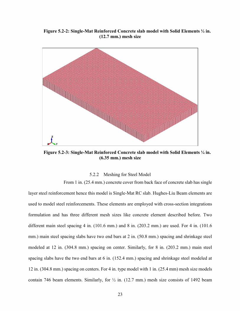
Figure 5.3-2: Single-mat reinforced concrete slab model with solid elements ½ in. (12.7 mm.)
Mesh size .......................................................................................................................... 23
Figure 5.3-3: Single-mat reinforced concrete slab model with solid elements ¼ in. (6.35 mm.)
Mesh size .......................................................................................................................... 23
Figure 5.3-4: Single layer reinforcement in 4 in. Type single-mat rc slab ................................... 25
Figure 5.3-5: Single layer reinforcement in 8 in. Type single-mat rc slab ................................... 25
Figure 5.4-1: Boundary conditions on the front and back face of slab ......................................... 30
Figure 5.4-2: Boundary conditions on the top and bottom face of the slab .................................. 31
Figure 5.5-1: Pressure versus volumetric strain curve for equation of state form 8 with compaction
for 11.6 ksi concrete .......................................................................................................... 35
Figure 5.5-2: Pressure versus volumetric strain curve for equation of state form 8 with compaction
for 5 ksi concrete ............................................................................................................... 36
Figure 6.1-1: Deflection history of constrained beam-bond parameter with juan and cib-fip
functions for cdr3 concrete model of 1 in. (24.4 mm.) Mesh model with constrained
lagrange in solid and experimental deflection for slab#2-rsc-r1-4in. With boundary
conditions of experiment setup. ..................... ERROR! BOOKMARK NOT DEFINED.
Figure 6.1-2: Deflection history of constrained beam-bond parameter with juan and cib-fip
functions for cdmr3 concrete material of 1 in. (24.4 mm.) Mesh model with constrained
lagrange in solid and experimental deflection for slab#2-rsc-r1-4in. With all boundary
conditions fixed. ............................................. ERROR! BOOKMARK NOT DEFINED.
x
Figure 6.2-1: Deflection comparison between ncoup parameter of constrained beam-bond
parameter with juan function for cdr3 concrete model of 1 in. (24.4 mm.) Mesh model with
experimental deflection for slab#4-rsc-r2-4in. ................................................................. 39
Figure 6.2-2: Deflection comparison between ncoup parameter of constrained beam-bond
parameter with juan function for cdr3 concrete model of 1 in. (24.4 mm.) Mesh model with
experimental deflection for slab#12-rsc-r2-8in. ............................................................... 40
Figure 6.2-3: Deflection comparison between ncoup parameter of beam-bond parameter with juan
function for cdr3 concrete model of 1 in. (24.4 mm.) Mesh model with experimental
deflection for slab#1-hsc-v2-4in. ...................................................................................... 41
Figure 6.2-4: Deflection comparison between ncoup parameter of constrained beam-bond
parameter with juan function for cdr3 concrete model of 1 in. (24.4 mm.) Mesh model with
experimental deflection for ............................................................................................... 41
Figure 6.2-5: Deflection comparison between ncoup parameter of constrained beam-bond
parameter with ceb-fip function for cdr3 concrete model of 1 in. (24.4 mm.) Mesh model
with experimental deflection for slab#12-rsc-r2-8in. ....................................................... 43
Figure 6.2-6: Deflection comparison between ncoup parameter of beam-bond parameter with cip-
fip function for cdr3 concrete model of 1 in. (24.4 mm.) Mesh model with experimental
deflection for slab#1-hsc-v2-4in. ...................................................................................... 44
Figure 6.2-7: Deflection comparison between ncoup parameter of constrained beam-bond
parameter with ceb-fip function for cdr3 concrete model of 1 in. (24.4 mm.) Mesh model
with experimental deflection forslab#11-hsc-v6-4in. ....................................................... 45
Figure 6.2-8: Deflection comparison between ncoup parameter of constrained beam-bond
parameter with ceb-fip-s3 function for cdr3 concrete model of 1 in. (24.4 mm.) Mesh model
with experimental deflection for slab#4-rsc-r2-4in. ......................................................... 46
Figure 6.2-9: Deflection comparison between ncoup parameter of constrained beam-bond
parameter with ceb-fip-s3 function for cdr3 concrete model of 1 in. (24.4 mm.) Mesh model
with experimental deflection for slab#12-rsc-r2-8in. ....................................................... 47
Figure 6.2-10: Deflection comparison between ncoup parameter of beam-bond parameter with cip-
fip-s3 function for cdr3 concrete model of 1 in. (24.4 mm.) Mesh model with experimental
deflection for slab#1-hsc-v2-4in. ...................................................................................... 48
xi
Figure 6.2-11: Deflection comparison between ncoup parameter of constrained beam-bond
parameter with ceb-fip-s3 function for cdr3 concrete model of 1 in. (24.4 mm.) Mesh model
with experimental deflection forslab#11-hsc-v6-4in. ....................................................... 49
Figure 6.3-1 : Deflection comparison between 1 in. (25.4 mm.) And 0.5 in. (12.7 mm.) For
constrained lagrange and beam in solid with no defined function and juan function with
experimental deflection for slab#1– hsc-v1-4in. .............................................................. 50
Figure 6.3-2: Deflection comparison between 1 in. (25.4 mm.) And 0.5 in. (12.7 mm.) For ceb-fip
and ceb-fip-s3 functions and experimental deflection for slab#1– hsc-v1-4in. ................ 51
Figure 6.3-3: Deflection comparison between 1 in. (25.4 mm.) And 0.5 in. (12.7 mm.) For
constrained lagrange and beam in solid with no defined function and juan function with
experimental deflection for slab#3– hsc-v2-4in. .............................................................. 52
Figure 6.3-4: Deflection comparison between 1 in. (25.4 mm.) And 0.5 in. (12.7 mm.) For ceb-fip
and ceb-fip-s3 functions and experimental deflection for slab#3– hsc-v2-4in. ................ 53
Figure 6.3-5: Deflection comparison between 1 in. (25.4 mm.) And 0.5 in. (12.7 mm.) For
constrained lagrange and beam in solid with no defined function and juan function with
experimental deflection for slab#5– hsc-v3-4in. .............................................................. 54
Figure 6.3-6: Deflection comparison between 1 in. (25.4 mm.) And 0.5 in. (12.7 mm.) For ceb-fip
and ceb-fip-s3 functions and experimental deflection for slab#5– hsc-v3-4in. ................ 55
Figure 6.3-7: Deflection comparison between slab#1 vs. Slab#5 for ceb-fip and ceb-fip-s3
functions and experimental deflection for 1in. (25.4 mm) mesh size. .............................. 56
Figure 6.3-8: Deflection comparison between 1 in. (25.4 mm.) And 0.5 in. (12.7 mm.) For
constrained lagrange and beam in solid with no defined function and juan function with
experimental deflection for slab#7– hsc-v4-8in. .............................................................. 57
Figure 6.3-9: Deflection comparison between 1 in. (25.4 mm.) And 0.5 in. (12.7 mm.) For ceb-fip
and ceb-fip-s3 functions and experimental deflection for slab#7– hsc-v4-8in. ................ 57
Figure 6.3-10: Deflection comparison between 1 in. (25.4 mm.) And 0.5 in. (12.7 mm.) For
constrained lagrange and beam in solid with no defined function and juan function with
experimental deflection for slab#9– hsc-v5-8in. .............................................................. 58
Figure 6.3-11: Deflection comparison between 1 in. (25.4 mm.) And 0.5 in. (12.7 mm.) For ceb-
fip and ceb-fip-s3 functions and experimental deflection for slab#9– hsc-v5-8in. .......... 59
xii
Figure 6.3-12: Deflection comparison between slab#7 vs. Slab#9 for ceb-fip and ceb-fip-s3
functions and experimental deflection for 1in. (25.4 mm) mesh size. .............................. 60
Figure 6.3-13: Deflection comparison between 1 in. (25.4 mm.) And 0.5 in. (12.7 mm.) For
constrained lagrange and beam in solid with no defined function and juan function with
experimental deflection for slab#11– hsc-v6-8in. ............................................................ 61
Figure 6.3-14: Deflection comparison between 1 in. (25.4 mm.) And 0.5 in. (12.7 mm.) For ceb-
fip and ceb-fip-s3 functions and experimental deflection for slab#11– hsc-v6-8in. ........ 62
Figure 6.4-1: Deflection comparison between 1 in. (25.4 mm.) And 0.5 in. (12.7 mm.) For
constrained lagrange and beam in solid with no defined function and juan function with
experimental deflection for slab#2– rsc-r1-4in. ................................................................ 63
Figure 6.4-2: Deflection comparison between 1 in. (25.4 mm.) And 0.5 in. (12.7 mm.) For ceb-fip
and ceb-fip-s3 functions and experimental deflection for slab#1– rsc-r1-4in. ................. 64
Figure 6.4-3: Deflection comparison between 1 in. (25.4 mm.) And 0.5 in. (12.7 mm.) For
constrained lagrange and beam in solid with no defined function and juan function with
experimental deflection for slab#4– rsc-r2-4in. ................................................................ 65
Figure 6.4-4: Deflection comparison between 1 in. (25.4 mm.) And 0.5 in. (12.7 mm.) For ceb-fip
and ceb-fip-s3 functions and experimental deflection for slab#4– rsc-r2-4in. ................. 66
Figure 6.4-5: Deflection comparison between 1 in. (25.4 mm.) And 0.5 in. (12.7 mm.) For
constrained lagrange and beam in solid with no defined function and juan function with
experimental deflection for slab#6– rsc-r3-4in. ................................................................ 67
Figure 6.4-6: Deflection comparison between 1 in. (25.4 mm.) And 0.5 in. (12.7 mm.) For ceb-fip
and ceb-fip-s3 functions and experimental deflection for slab#6– rsc-r3-4in. ................. 68
Figure 6.4-7:Deflection comparison between slab#2 vs. Slab#4 vs. Slab#6 for constrained lagrange
and beam in solid with no defined function and juan function with experimental deflection
for0.5 in. (12.7 mm.) Mesh size. ...................................................................................... 69
Figure 6.4-8 : Deflection comparison between 1 in. (25.4 mm.) And 0.5 in. (12.7 mm.) For
constrained lagrange and beam in solid with no defined function and juan function with
experimental deflection for slab#8– rsc-r4-8in. ................................................................ 70
Figure 6.4-9 : Deflection comparison between 1 in. (25.4 mm.) And 0.5 in. (12.7 mm.) For ceb-
fip and ceb-fip-s3 functions and experimental deflection for slab#8– rsc-r4-8in. ............ 71
xiii
Figure 6.4-10: Deflection comparison between 1 in. (25.4 mm.) And 0.5 in. (12.7 mm.) For
constrained lagrange and beam in solid with no defined function and juan function with
experimental deflection for slab#10– rsc-r5-8in. .............................................................. 72
Figure 6.4-11 : Deflection comparison between 1 in. (25.4 mm.) And 0.5 in. (12.7 mm.) For ceb-
fip and ceb-fip-s3 functions and experimental deflection for slab#10– rsc-r5-8in. .......... 73
Figure 6.4-12: Deflection comparison between 1 in. (25.4 mm.) And 0.5 in. (12.7 mm.) For
constrained lagrange and beam in solid with no defined function and juan function with
experimental deflection for slab#12– rsc-r6-8in. .............................................................. 74
Figure 6.4-13: Deflection comparison between 1 in. (25.4 mm.) And 0.5 in. (12.7 mm.) For ceb-
fip and ceb-fip-s3 functions and experimental deflection for slab#12– rsc-r6-8in. .......... 75
Figure 6.4-14: comparison between slab#2 vs. Slab#4 vs. Slab#6 for constrained lagrange and
beam in solid with no defined function and juan function with experimental deflection
for0.5 in. (12.7 mm.) Mesh size. ...................................................................................... 76
Figure B-8.1-1 : Average pressure-time history for slab # 1. ....................................................... 87
Figure B-8.1-2: Average pressure-time history for slab # 2. ........................................................ 87
Figure B-8.1-3: Average pressure-time history for slab # 3. ........................................................ 88
Figure B-8.1-4: Average pressure-time history for slab # 4. ........................................................ 88
Figure B-8.1-5: Average pressure-time history for slab # 5. ........................................................ 89
Figure B-8.1-6: Average pressure-time history for slab # 6. ........................................................ 89
Figure B-8.1-7: Average pressure-time history for slab # 7. ........................................................ 90
Figure B-8.1-8: Average pressure-time history for slab # 8. ........................................................ 90
Figure B-8.1-9: Average pressure-time history for slab # 9. ........................................................ 91
Figure B-8.1-10: Average pressure-time history for slab # 10. .................................................... 91
Figure B-8.1-11: Average pressure-time history for slab # 11. .................................................... 92
Figure B-8.1-12: Average pressure-time history for slab # 12. .................................................... 92
Figure D - 8.1-1 : Input and output control parameters ................................................................ 95
Figure D- 8.1-2: iInput parameters for concrete damage model release 3 for high-strength concrete
........................................................................................................................................... 96
Figure D - 8.1-3: Input parameters generated by concrete damage model release 3 for high- strength
concrete. ............................................................................................................................ 97
xiv
Figure D - 8.1-4 : Input parameters for concrete damage model release 3for normal-strength
concrete ............................................................................................................................. 98
Figure D - 8.1-5: Input parameters generated by concrete damage model release 3 for high-strength
concrete ............................................................................................................................. 99
Figure D - 8.1-6: Input parameters for plastic-kinematic model for high-strength concrete ...... 100
Figure D - 8.1-7: Input parameters for plastic-kinematic model for normal-strength concrete . 100
Figure D - 8.1-8: Input parameters for constrained lagrange in solid formulation .................... 100
Figure D- 8.1-9: Input parameters for constrained beam in solid formulation with no user defined
function. .......................................................................................................................... 100
Figure D - 8.1-10: Input parameters for constrained beam in solid formulation with user defined
function. .......................................................................................................................... 101
Figure D - 8.1-11: Input function for ceb-fip function for high-strength concrete. .................... 101
Figure D - 8.1-12 : Input function for ceb-fip function for normal-strength concrete................ 102
Figure D - 8.1-13 : Input function for ceb-fip-s3 function for high-strength concrete. .............. 103
Figure D - 8.1-14: Input function for ceb-fip-s3 function for normal-strength concrete. ........... 104
Figure D - 8.1-15: Input function for juan function for high-strength concrete. ........................ 105
Figure D - 8.1-16: Input function for juan function for normal-strength concrete. .................... 106
xv
LIST OF TABLES
Table 4-1: Experimental program schedule .................................................................................. 15
Table 4-2 : Slab designation details foe experimental program. .................................................. 16
Table 6-1: Ncoup parameter variation results for juan function ................................................... 41
Table 6-2: Ncoup parameter variation results for CEB-FIP function ........................................... 42
Table 6-3: Ncoup parameter variation results for CEB-FIP-s3 function ...................................... 47
Table 6-4: Numerical simulation results for slab#1 HSC-V1-4in. ............................................... 51
Table 6-5: Numerical simulation results for Slab#3, HSC-V2-4in............................................... 52
Table 6-6: Numerical simulation results for Slab#5, HSC-V3-4in............................................... 54
Table 6-7: Numerical simulation results for Slab#7, HSC-V4-8in............................................... 57
Table 6-8: Numerical simulation results for Slab#9, HSC-V5-8in............................................... 58
Table 6-9: Numerical simulation results for Slab#11, HSC-V6-8in............................................. 61
Table 6-10: Numerical simulation results for Slab#2, RSC-R1-4in. ............................................ 63
Table 6-11: Numerical simulation results for Slab#4, RSC-R2-4in. ............................................ 65
Table 6-12: Numerical simulation results for Slab#6, RSC-R3-4in. ............................................ 67
Table 6-13: Numerical simulation results for Slab#8, RSC-R4-8in. ............................................ 70
Table 6-14: Numerical simulation results for Slab#10, RSC-R5-8in. .......................................... 72
Table 6-15: Numerical simulation results for Slab#12, RSC-R6-8in. .......................................... 74
Table 7-1: Analytical and experimental peak slab deflection summary for high strength slabs for
1 in. Mesh size. ..................................................................................................................... 77
Table 7-2: Analytical and experimental peak slab deflection summary for high strength slabs for
1/2 in. Mesh size. .................................................................................................................. 78
Table 7-3: Percentage comparison of peak slab deflections with the experimental value for high
strength slabs for 1in. Mesh size. .......................................................................................... 78
Table 7-4: Percentage comparison of peak slab deflections with the experimental value for high
strength slabs for ½ in. Mesh size. ........................................................................................ 79
Table 7-5: Analytical and experimental peak slab deflection summary for regular strength slabs
for 1 in. Mesh size. ................................................................................................................ 80
Table 7-6: Analytical and experimental peak slab deflection summary for regular strength slabs
for 1/2 in. Mesh size.............................................................................................................. 81
xvi
Table 7-7: Percentage change in peak slab deflection when the mesh size was reduced from 1 in.
(25.4mm.) To ½ in. (12.7 mm.) For r strength slabs. ........................................................... 81
Table 7-8: Percentage comparison of peak slab deflections with the experimental value for regular
strength slabs for ½ in. Mesh size ......................................................................................... 82
Table 7-9: Percentage change in peak slab deflection when the mesh size was reduced from 1 in.
(25.4mm.) To ½ in. (12.7 mm.) For high strength slabs. ...................................................... 83
Table 7-10: Percentage change in peak slab deflection when the mesh size was reduced from 1 in.
(25.4mm.) To ½ in. (12.7 mm.) For regular strength slabs. ................................................. 83
Table C- 0-1: Input parameters for concrete damage model release 3 ......................................... 93
Table C- 0-2: Input parameters for plastic kinematic model for steel rebar ................................. 94

xvii
ACKNOWLEDGEMENT
I would like to take this opportunity to thank all those people who helped me to complete
this thesis.
It is with immense gratitude that I acknowledge the guidance and encouragement of my
advisor, Dr. Thiagarajan Ganesh. Throughout the length of my education and research at
University of Missouri – Kansas City, he has constantly supported me and has given me valuable
insights which made the completion of this thesis possible.
I am grateful to Dr. Ceki Halmen and Dr. Zhiqiang Chen for serving as the members on
the supervisory committee and for providing their valuable input and suggestions. I am thankful
to the School of Computing and Engineering for providing the necessary facilities in order to
pursue the research studies for this thesis.
I would like to express my deepest gratitude to my senior lab mates Hamad, Lorry and
Jade. Their inspiring research work motivated me and was vital in developing my interest in
performing research and provided me the opportunity to learn from them. I am thankful for them
in keeping a peaceful and friendly environment in the lab which was motivating in performing my
research. I owe my sincere thanks to my dear friends Raju, Soham, Maitrey, Plamond and Sanket
for their moral support throughout my studies at UMKC. Their friendships were instrumental in
my desire to achieve my goals.
I also wish to thank all my family members and friends for their support. Most importantly,
I owe my loving thanks and sincere appreciation to my parents Ashok and Ashwini Iwalekar.
Throughout my studies abroad they never failed in their encouragement, patience and
understanding. To them I dedicate this thesis.

1
CHAPTER 1. INTRODUCTION
1.1 An overview on Blast Effects on Structures
In recent times, instances occur where civilian structures were under aggressive
attack by means of blast or explosives. The attack on the World Trade Center on February 26th,
1993, in New York, and the bombing which destroyed the Alfred P. Murrah Building on April
19th, 1995, in Oklahoma City, are two primary examples of attacks that occurred during the past
couple of decades. These attacks have led to the need for more blast resistant designs for civilian
structures, as the reason that lives were lost in these attacks was due to the inability of these
structures to resist blast loading. When considering blast loading, a new efficient design approach
should be adopted in order to minimize the damage specifically to civilian structures. In past,
military structures have been designed for blast loading. In recent history, government and civilian
buildings have increasingly become potential threats to attacks. Therefore, design procedures and
guidelines, which are easy to implement for civilian structures need to be designed and produced.
DoD Minimum Antiterrorism Standards for Buildings, UFC 4-010-01, is one such design
guideline, which has been established for stating the minimum level of protections against terrorist
attacks for the Department of Defense structures [5]. Furthermore, these guidelines outline
feasible ways to implement blast protection in military structures. It is imperative that adaptations
for the application of blast mitigation methodology of civilian structures from military structures
are be done. Blast-effect mitigation is the reduction in the severity of effects of an explosion on a
structure resulting from having taken specific blast hardening measures in order to reduce or
eliminate the effects of an explosion, according to the National Research Council [6]. In order to
find the best alternative for the design of building components, such as wall panels, columns slabs,
2
beams etc., expensive research has been carried out. Structures like offices, research facilities,
education institutions etc., which are occupied by large human populations and are more prone to
aggressor attacks, such consideration state becomes critical.
1.2 Significance of Studying Blast Effects on Reinforced Concrete Slabs
The internal and external structure of buildings like walls and columns can get damaged
due to an explosion, within or near the structure, leading to the partial disability or the complete
failure of fire-safety and life-safety systems. Increasing the resistance of the structure to blast
loading thereby strengthening the structure itself, can be one of the solutions. However, this
adoption can prove to be expensive when it is implemented on a large scale. The study of the blast
damage caused to the Alfred P. Murrah building during the Oklahoma City Bombing, done by
Mlakar et al. [7], has evaluated the effect of the blast caused by the truck bomb on the buildings
structural frame. Columns in the surrounding areas of the blast underwent major damage, and the
blast induced pressures severely affected the floor slabs above and below the blast epicenter. This
caused maximum displacement of 9.3 inches in an upward direction, between, above and below
slabs which lead to the collapse of the slab. As reinforced concrete slabs are one of the most basic
type of slabs designed today, their strengthening is required. Reinforced concrete wall panels
designed for blast loading are one of the additional protective measures that act as a shield for the
main structure. Studies of dynamic behavior of reinforced concrete slabs, under high blast loads
of short duration, become necessary and is the motivation behind this study. Around the world,
structural engineers use advanced analysis methods to ensure resistance to blast loading on their
designed structures. For predicting blast loads and response of structures to blast loading,
experimental studies, theoretical analysis and advanced numerical simulation can be used for the
evaluation of behavior of civilian structure to blast loading.
3
1.3 Proposed Solution
In order to predict the effects of blast and the quantification of structural
response to blast and its interaction with the structures, coming up with theories and experiments
to test these theories are necessary. For estimating the response of a structure to an explosion,
results obtained for these theories and experiments can be used. Even though the computational
approach is far less expensive than the experimental approach, experimental studies are requiring
for the validation of this computational approach. Numerous experiments are performed by various
military organizations on military structures. The application of these experiments on civilian
structures can and needs to be studied and investigated.
This study involves the numerical study of the reinforced concrete slab, an
important component of any structural system. The comparison of the results of high strength and
normal strength material from experiments done previously will be utilized and will then later be
compared with the numerical study. Finite Element Method (FEM) is used to analyze the
effectiveness of the strengthened slabs against blast loading. LS-DYNA®, a non-linear transient
dynamic finite element analysis program code, is employed in this study. This program has various
advantageous features of defining pressure-time histories generated in the blast event and later
analyzing the model. Commercially available material models are used to define concrete and steel
materials, which are Concrete Damage Model Release 3 for concrete and plastic kinematic model
for steel. In order to define bond between the concrete and the steel, both perfect bonds employing
Lagrange in solid, and bond slip under Beam in solid, are used for both material strengths [1].
Comparison of the two bond types is the focus of this study.
At the U.S. Army Engineering Research and Development Center in Vicksburg,
MS, initial experiment investigation was carried out on twelve single-mat reinforced concrete RC
4
slab panels. The slabs consisted of two sets of panels; the first one consisted of High Strength
Concrete reinforced with High Strength Steel Reinforcing bars (HSC-V) and the other one was of
Normal Strength Concrete reinforced with Normal Strength Steel Reinforcing bars (NSC-R). The
twelve sets of concrete had two different sets of reinforcement ratios, one set had #3 bars spaced
at 4 inch (101.6 mm.) and the other set had #3 bars spaced at 8 inches (203.2 mm.). The twelve
slabs were subjected to pressure conditions equivalent to those in a blast load which were generated
using a Blast Load Simulator. The experimental data that was collected for this testing included
measurement of the slab displacement, slab strain and slab damage/crack patterns. The
displacement at mid-span was measured with lasers and accelerometers during the testing, using
pressure versus time history at 6 locations on the slabs. Strains were measured at two locations
using strain gages, photos and videos documented the locations and severity of damage crack
patterns for each slab.
1.4 Thesis Organization
The thesis is organized as follows:
1. Chapter 1 introduces the subject of this thesis, which is about experimental validation of
reinforced concrete single mat slabs subjected to blast loading and finite element analysis.
2. Chapter 2 includes the literature review for the study of this thesis.
3. Chapter 3 includes the scope and the objective of this thesis.
4. Chapter 4 describes experimental investigation. Dr. Ganesh Thiagarajan, the Principal
Investigator for this project, conducted this experiment at U.S. Army Engineer Research
and Development Center at Vicksburg, MS. That experiment is not a part of this thesis;
therefore, it is described in detail. The information collected from this experiment includes
the types of reinforced concrete panels, the equipment used for applying the blast pressures
5
and the various types of data collected. Numerical analysis is performed using the data
obtained from this experiment.
5. Chapter 5 includes details of the reinforced concrete slabs numerical modeling, the
geometry of the finite element models, the various mesh sizes adopted, the material models
used for modeling the steel and the concrete from program are described in this chapter.
6. Chapter 6 includes the results obtained from the numerical simulations performed and the
observations of such. The simulations are done using the LS-DYNA® program.
7. Chapter 7 includes the examination and deliberation of the results presented in Chapter 6.
8. Chapter 8 includes the conclusions that were drawn from this study and are based on the
analysis of the test results. This chapter also includes details and recommendations for
future work.
6
CHAPTER 2. LITERATURE SURVEY
In the research world, efforts have been made to improve the blast resistance of
buildings. The primary focus has been to develop effective methods which can be easily
implemented. The goal would be to produce design protective technologies which are readily
available for both design and structural engineers.
A numerical analysis on the dynamic behavior of RC slabs under blast loading
was performed by Hao and Zhongxian [9]. They discussed the influence of various structural and
geometric parameters of RC slabs under blast loading in their study. Among their testing were the
concrete strength, the reinforcement ratio and the dimension of the slab. They remarked that
reinforced concrete (RC) slab resistance to blast loading increased with an increase in slab
thickness.
To improve the blast resistance of buildings, Crawford and Lan [8] used
different engineering techniques as solutions. They carried out studies of numerical modeling and
testing of the effects of blasts and impacts. From their study, they recommended the use of high-
fidelity physics-based (HFPB) finite element models. Their challenge was to develop a model
which would provide a refined representation of the behavior during blast loading. HFPB models
fulfilled this challenge and validation was stated as being significant. Ductility and plastic
behavior, use of standard material in a non-standard way and shock relative behavior are the three
primary design benchmarks described in their work.
The method of finite element analysis was used by Mosalam and Mosallam [10]
to develop computational models of reinforced concrete slabs (RC) under blast loading. Non-linear
transient analysis was carried out, by them, in order to investigate and compare the behavior
between retrofitted RC slabs with carbon fiber reinforced (CFRP) polymer slabs to as-built RC
7
slabs when subjected to blast loading. The efficiency of CFRP polymer slabs was stated in this
study noting a reduction of the displacement from 40% to 70%, in comparison to as-built slabs.
Computational models were verified using experimental data.
Agardh [11] presented a study of FE model simulation on fiber reinforced
concrete and the experimental results were focused on the behavior of these models under transient
dynamic loads. The comparison of the experiments on conventional reinforced concrete slabs and
steel fiber were carried out in this study with the blast experiments performed in a shock tube.
Validation of these results were done using two codes: LS-DYNA® and ABAQUS®/explicit with
Winfrith concrete model for LS-DYNA® and Constitutive model for brittle cracking in
ABAQUS®/Explicit as concrete models. Accurate results were obtained for the use of parameters
prediction of failure loads and for the displacement for low loads. The exclusion of the strain rate
effect was recommended in this study by stating that the distance between the slabs and the charge
was large, therefore causing the strain rate effect to be insignificant.
Due to the symmetry of the slabs Kuang [12] modeled only a quarter of three-
dimensional FE model of RC slabs that were subjected to blast loading and carried out numerical
simulation in LS-DYNA®. To model concrete material Johnson-Holmquist Concrete (H-J-C) [1]
model was used in this study to account for the damage and strain rate effect and the erosion
technique was used for modeling the spallation process. Effective prediction of the response of the
reinforced concrete section was noted in comparison between the blast test results and the
numerical simulation results.
For the purpose of analyzing responses of two-way reinforced concrete panels
which were subjected to blast loading, El-Dakhakhni [13] used and studied the validity of Single-
Degree-of-Freedom (SDOF) models which were developed in accordance to the guidelines of the
8
UFC 3-340-02 [6]. These RC panels had variations in dimensions, aspect and reinforcement ratios,
and support conditions. Finite element analysis was carried out in LS-DYNA® utilizing the
parameter generation capability of *MAT_CONCRETE_DAMAGE_REL3 (mat type 72R3)
model for the concrete material and PLASTIC_KINEMATIC (mat type 003) for the steel material
[1]. Razagpur (2006) had previously provided validation for these models. Results that were
obtained from these numerical simulations were compared to results obtained for the nonlinear
explicit finite-element (FE) analysis. Significant variations in the shear and deflection predictions
were observed. This study identified the many limitations of the SDOF models over the FE
analysis techniques. Above and beyond the SDOF model analysis parameters, the FE analysis
method can include different failure modes such as shear, bar slippage, etc., as well as material
strength enhancement due to strain rate effects. The results of this study noted the strong
advantages of FE analysis over the SDOF model analysis.
Significant research has been carried out in the last couple of decades in order
to accurately predict concrete material properties in finite element models developed for concrete
structures. In order to replicate the exact behavior in the finite element model, sophisticated
knowledge of the behavior of concrete structures is required. For this process, initial laboratory
experiments were conducted with control over the structural parameters. Data from the
experiments can then be used to calibrate the available computer models. A similar kind of
methodology was adopted by Malvar and Schwer [14]. They characterized the parameters of 45.6
MPa unconfined compressive strength concrete model parameters from laboratory tests. They then
implemented it with LS-DYNA® in commercial K & C concrete model [1]. The results obtained
from this study recommended the use of a model parameter generation capability of Mat72R3 by
using the unconfined compressive strength of the concrete as input.
9
Blast analysis was performed on 1.19m X 2.19m X 0.14m RC slabs by
Tanapornaweekit [12] employing 500kg TNT testing in Woomera, South Australia. For predicting
blast load properties, AIR3D and CONWEP computer programs were used. These predictions
were compared to results obtained by pressure transducers in test. For the purpose of numerical
simulation LS-DYNA® was used and the results obtained from the numerical simulations were
compared to the experimental results. In the numerical simulation, to define the concrete material
of the panel, *MAT_CONCRETE_DAMAGE_REL3 was used. This model takes account for
three failure surfaces which are: Maximum shear failure surface, residual surface and initial yield
surface. The advantage of this material model is that it has automatic parameter generation
capability for the input compressive strength of the concrete [1]. For this study, the compressive
strength of 40 MPa was used as input value, giving a total of 8 automatic parameters that were
generated. Three failure surfaces were considered in this material model and they are governed by
three equations which are discussed in this thesis. For the purpose of modeling the steel material,
model *MAT_PLASTIC_KINAMATIC was utilized [1]. For defining the bond between the steel
and concrete, a full bond between the two materials was assumed between nodes. The results of
the numerical simulation in FE reported that the maximum deflection was 30mm and the maximum
rebound deflection was 4 mm. This corresponds to the experimental difference of 17%.
Experimental results for the maximum and the rebound deflection were 36mm and 5mm
respectively.
The dynamic plastic damage model was adopted by Zhou and Kuznetsov [13]
in order to study and compare both ordinary reinforced and high-strength steel fiber reinforced
concrete slabs. This concert model is developed by taking reference form material models used in
separate researcher which are not part of their project and with equations of concrete strength
10
derived from static and dynamic material testing and parameters such as deflection of damage,
strain-rate effects and concrete strength envelope. The comparison gave understanding as to the
numerical simulation for t > 2ms gives lower value to peak deflection results, for t < 2ms
estimation of ultimate deflection is well with experimental records. This type of results is common
for both RC and the high strength Steel Fiber Reinforced Concrete (SFRC) slabs.
Shetye [2] performed numerical analysis on single-mat reinforced concrete
(RC) slabs in LS-DYNA® on 12 slabs. This study focused on the comparison of two commercially
available concrete material models. Interaction between the steel and the concrete of RC slabs
were modeled employing a perfect bond between them. Effect of mesh size model on finite element
analysis and the outcome of two different reinforcement ratios were also investigated in this study.
Increase in peak deflection, with decrease in mesh size for both concrete models, and on reduction
on reinforcement ratio, led to increased deflection by twice the amount are results stated in this
study with recommendation of Winfrith Concrete Model for both high and regular strength
concrete.
Literature review here indicated different types of approaches adopted for
investigating and analyzing blast mitigation techniques, which are evaluated using SDOF system
or finite element analysis system in order to study the effect of dynamic loading of short duration
on reinforced concrete slabs. This thesis including a similar combination of techniques which
involves two different material strength, two different mesh sizes, two separate reinforcement
ratios and two different bond interaction models between the steel and the concrete and
compression of experimental records to numerical analysis study performed to investigate
validation of numerical approach adopted.
11
CHAPTER 3. OBJECTIVE AND SCOPE
3.1 Problem Statement
To accurately predict the structural response to dynamic loading in finite
element modeling is a difficult task. Hence, it is necessary to include the exact material description
of material parameters through input parameters in model, which helps in capturing rapidly
changing material behavior in dynamic loading. In order to obtain accurate material properties, the
challenging task of comprehensive laboratory testing on materials needs to be performed. In order
to counter this challenge, the use of commercially available material models was employed for this
study, which accurately describe the response and behavior for developed FE slab models. Hence,
it becomes necessary to validate the results obtained from numerical simulation, which employed
commercial material models, to results obtained from experimental investigation.
3.2 Objectives
This thesis focuses on investigating blast loading on Reinforced Concrete
(RC) one-way slabs having a single layer of reinforcement. This is achieved by performing Finite
Element (FE) simulations which the results obtained from this simulation are then compared with
experimental data. The scope of the thesis is outlined as follows to achieve this goal.
1. To perform numerical analysis and modeling in LS-DYNA® program, by using data
from experimental investigation. This includes use of deflection-time history and
pressure-time histories records.
2. In LS-DYNA® program, create slab models identical to experimental investigation
with dimensions of 64 in. x 34 in. x 4in. (1652 mm. x 863 mm. x 101.6 mm.).
12
3. Mesh sizes of 1 in. (25.4 mm) having 4 elements through the slab thickness, ½ in. (12.7
mm.) having 8 elements through the slab thickness and ¼ in. (6.35 mm.) having 16
elements through the slab thickness, to be used in order to perform mesh analysis.
4. To use two different reinforcement ratios for each material combination, for
investigating study the effect of reinforcement ratio.
5. Two types of material combinations to be considered based on concrete strength to be
used, which involves normal strength concrete reinforced with normal strength steel
and high strength concrete reinforced with high strength steel.
6. Using Plastic Kinematic Model to model the steel and Concrete Damage Model
Release 3 to model the concrete in LS-DYNA® program.
7. Use Constrained Lagrange in Solid formulation to model prefect bond and Constrained
Beam in Solid formulation for bond-slip modelling between steel and concrete.
8. Comparison is made between two types of bond relations molded in LS-DYNA®
program are results are compared with experimental investigation to determine which
bond formulation is accurate to predict outcome of analysis. Thus, validating bond
relation between steel and concrete and avoiding expensive blast experiments is the
goal of this study.
3.3 Tasks
Task 1: To utilize information of experimental investigation on twelve
Reinforced Concrete (RC) slab panels performed earlier, which was not part on this study. This
experimental investigation on twelve slabs had a combination of normal strength concrete with
normal reinforced Concrete (RSC-R) and high strength concrete with high strength steel (HSC-V)
slab panels, each with dimensions of 64 in. (1625 mm.) X 34in. (864 mm.) X 4 in. (101.6 mm.)
13
and consisted of single-mat reinforcement. This combination of normal strength concrete (5 ksi,
34.47 MPa) with normal strength steel (60 ksi, 413.68 MPa) and high strength concrete (15 ksi,
103.42 MPa) reinforced with high strength vanadium steel (83 ksi, 572.26 MPa) were loaded with
blast pressure within a Shock Tube for experimental investigations. On six different regions on the
slab, pressure and impulse histories were recorded and deflections were measured using a laser
device which was placed at the center of the slab. The strain history was recorded employing strain
gauges located at quarter points of the unloaded face of the slab.
Task 2: Material of concrete slabs were modelled using commercially
available material models. Concrete Damage Model Release 3 is used for concrete while steel is
modeled using Plastic Kinematic Model. The Bond between the concrete and steel were model
using perfect bond relations and bond-slip mechanisms. Lagrange in solid formulation was used
for modelling perfect bond whereas Beam in solid formulation was used for modeling bond-slip.
In bond-slip formulation, three custom functions are used defining bond-slip law. CEB-FIP, CEB-
FIP-S3 and function for bond-slip law proposed by Juan are used in this study. Mesh size analysis
was also carried out to investigate its effect on FE analysis. These are explained in the following
chapters. Verification of FE analysis results to experimental results was based on deflection history
records of slab when subjected to blast pressures and impulses that the experimental specimen was
subjected to.
Task 3: The effect of the reinforcement ratio was also investigated with two
different reinforcement ratios, #3 bars spaced at 4in. c/c (101.6 mm.) in the longitudinal direction
(reinforcement ratio = 0.68%) for first set of six slabs and #3 bars spaced at 8in. c/c in the
longitudinal direction (reinforcement ratio = 0.46%) for the remaining six slabs for the main steel.
These two set of models are referred to as 4in and 8in models respectively. The ratio of the

14
shrinkage of the steel is the same for all 12 slabs, #3 bars spaced at 8in. c/c in the longitudinal
direction (reinforcement ratio = 0.46%).
The outcome of this study is used for recommendations for the custom
function to be used for defining bond-slip low for both material strengths used in modeling for
numerical formulation and are validated used experimental results, for blast loading in future.
15
CHAPTER 4. EXPERIMENTAL INVESTIGATION
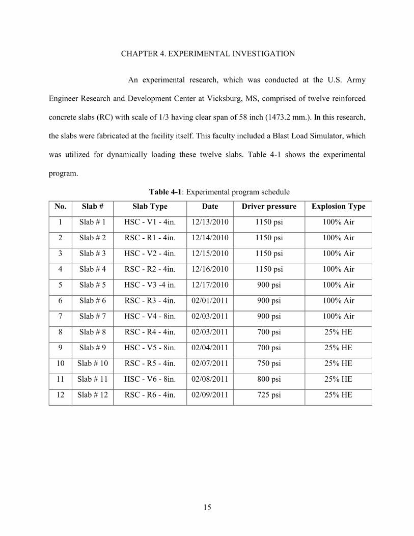
An experimental research, which was conducted at the U.S. Army
Engineer Research and Development Center at Vicksburg, MS, comprised of twelve reinforced
concrete slabs (RC) with scale of 1/3 having clear span of 58 inch (1473.2 mm.). In this research,
the slabs were fabricated at the facility itself. This faculty included a Blast Load Simulator, which
was utilized for dynamically loading these twelve slabs. Table 4-1 shows the experimental
program.
Table 4-1: Experimental program schedule
No. Slab # Slab Type Date Driver pressure Explosion Type
1 Slab # 1 HSC - V1 - 4in. 12/13/2010 1150 psi 100% Air
2 Slab # 2 RSC - R1 - 4in. 12/14/2010 1150 psi 100% Air
3 Slab # 3 HSC - V2 - 4in. 12/15/2010 1150 psi 100% Air
4 Slab # 4 RSC - R2 - 4in. 12/16/2010 1150 psi 100% Air
5 Slab # 5 HSC - V3 -4 in. 12/17/2010 900 psi 100% Air
6 Slab # 6 RSC - R3 - 4in. 02/01/2011 900 psi 100% Air
7 Slab # 7 HSC - V4 - 8in. 02/03/2011 900 psi 100% Air
8 Slab # 8 RSC - R4 - 4in. 02/03/2011 700 psi 25% HE
9 Slab # 9 HSC - V5 - 8in. 02/04/2011 700 psi 25% HE
10 Slab # 10 RSC - R5 - 4in. 02/07/2011 750 psi 25% HE
11 Slab # 11 HSC - V6 - 8in. 02/08/2011 800 psi 25% HE
12 Slab # 12 RSC - R6 - 4in. 02/09/2011 725 psi 25% HE
16
4.1 Materials
Dr. Ganesh Thiagarajan was the Principal Investigator for this project when
this experiment was conducted. High-strength materials were compared to conventional materials
in this study. Resistance of both types of materials, under dynamic loads, were examined. The
overall dimensions for the single-mat slab panels tested are 64 in. (1625 mm.) X 34in. (864 mm.)
X 4 in. (101.6 mm.) which are 1/3 scale models. Based on strength two of material combinations
which were used are designated as “HSC-V” for High-Strength material combination and “RSC-
R” for Normal-Strength material combination. Table 4-1-1 gives detailed description of slab-
designation.
Table 4-2 : Slab designation details foe Experimental Program.
Designation Description Material strength
HSC High-strength concrete 15 ksi (103.42MPa)
RSC Regular-strength concrete 5 ksi (34.47MPa)
V# Vanadium steel rebar 83 ksi (572.26MPa)
R# Grade 60 Conventional rebar 60 ksi (413.68MPa)
4 in. Longitudinal bars spacing -
8 in. Longitudinal bars spacing -
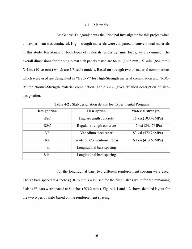
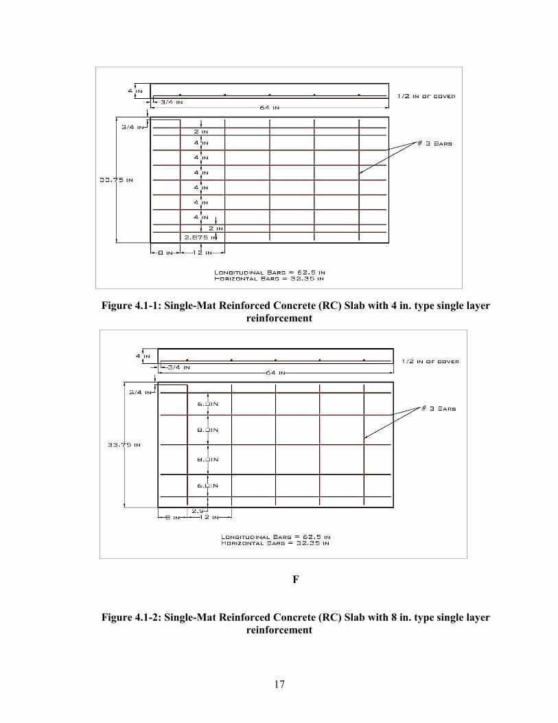
For the longitudinal bars, two different reinforcement spacing were used.
The #3 bars spaced at 4 inches (101.6 mm.) was used for the first 6 slabs while for the remaining
6 slabs #3 bars were spaced at 8 inches (203.2 mm.). Figure 4-1 and 4-2 shows detailed layout for
the two types of slabs based on the reinforcement spacing.
17
Figure 4.1-1: Single-Mat Reinforced Concrete (RC) Slab with 4 in. type single layer
reinforcement
F
Figure 4.1-2: Single-Mat Reinforced Concrete (RC) Slab with 8 in. type single layer
reinforcement
18
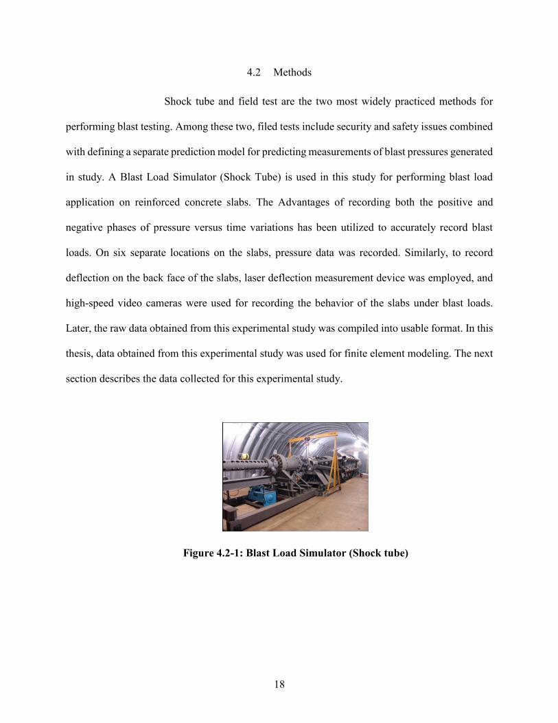
4.2 Methods
Shock tube and field test are the two most widely practiced methods for
performing blast testing. Among these two, filed tests include security and safety issues combined
with defining a separate prediction model for predicting measurements of blast pressures generated
in study. A Blast Load Simulator (Shock Tube) is used in this study for performing blast load
application on reinforced concrete slabs. The Advantages of recording both the positive and
negative phases of pressure versus time variations has been utilized to accurately record blast
loads. On six separate locations on the slabs, pressure data was recorded. Similarly, to record
deflection on the back face of the slabs, laser deflection measurement device was employed, and
high-speed video cameras were used for recording the behavior of the slabs under blast loads.
Later, the raw data obtained from this experimental study was compiled into usable format. In this
thesis, data obtained from this experimental study was used for finite element modeling. The next
section describes the data collected for this experimental study.
Figure 4.2-1: Blast Load Simulator (Shock tube)
19
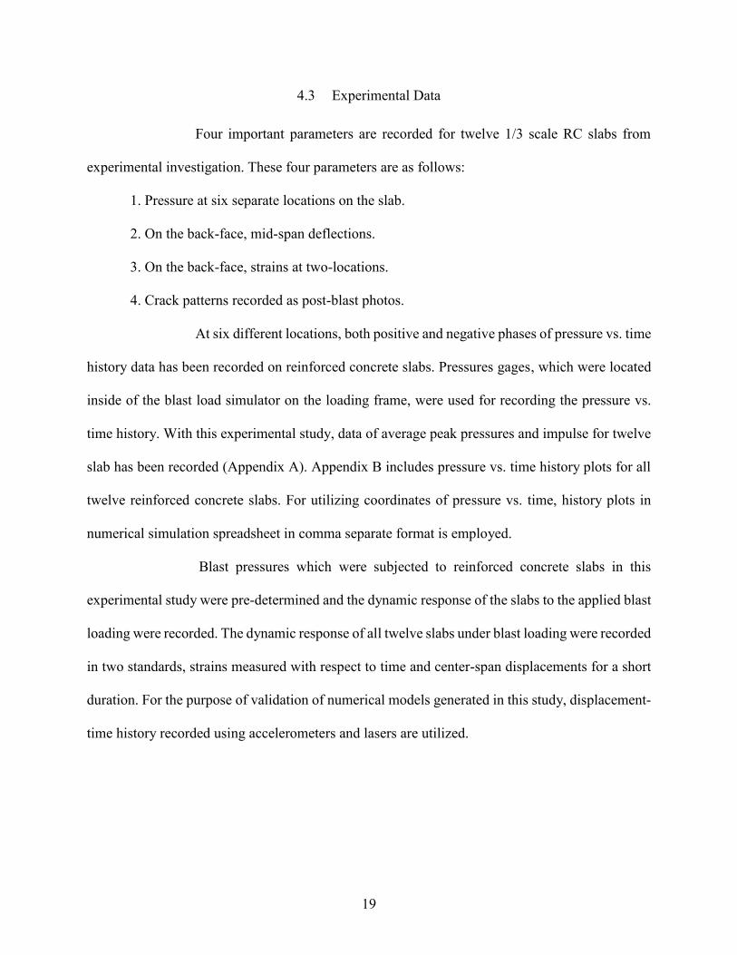
4.3 Experimental Data
Four important parameters are recorded for twelve 1/3 scale RC slabs from
experimental investigation. These four parameters are as follows:
1. Pressure at six separate locations on the slab.
2. On the back-face, mid-span deflections.
3. On the back-face, strains at two-locations.
4. Crack patterns recorded as post-blast photos.
At six different locations, both positive and negative phases of pressure vs. time
history data has been recorded on reinforced concrete slabs. Pressures gages, which were located
inside of the blast load simulator on the loading frame, were used for recording the pressure vs.
time history. With this experimental study, data of average peak pressures and impulse for twelve
slab has been recorded (Appendix A). Appendix B includes pressure vs. time history plots for all
twelve reinforced concrete slabs. For utilizing coordinates of pressure vs. time, history plots in
numerical simulation spreadsheet in comma separate format is employed.
Blast pressures which were subjected to reinforced concrete slabs in this
experimental study were pre-determined and the dynamic response of the slabs to the applied blast
loading were recorded. The dynamic response of all twelve slabs under blast loading were recorded
in two standards, strains measured with respect to time and center-span displacements for a short
duration. For the purpose of validation of numerical models generated in this study, displacement-
time history recorded using accelerometers and lasers are utilized.
20
CHAPTER 5. NUMERICAL MODELING IN LS-DYNA®
The study of numerical simulation is carried out in LS-DYNA®. For this
numerical analysis a numerical model of Single-Mat RC slab was developed. This model was
subjected to blast load to replicate the experiments performed. To achieve the primary objective
of comparing different bond relations between steel and concrete against blast loading, results
achieved form numerical simulations are compared to records of high-strength reinforced and
normal-strength reinforced concrete slabs of experiments. This numerical study performs
validation of different pre-defined bond relation between reinforcing steel and concrete materials
of two different strengths. This chapter discusses significance of LS-DYNA® for numerical
simulations, constitutive material model, ability to define bond relations by user between
reinforcement steel and concrete, boundary conditions and blast load application.
5.1 Significance of Numerical Modeling in LS-DYNA®
LS-DYNA® is a highly non-linear finite element program, which uses explicit
time integration for performing transient dynamic finite element analysis. This program provides
various material models and elements formulation in its material and element library [1]. A single-
mat reinforced concrete slab model was developed in LS-DYNA® and finite element analysis was
carried out.
Accurate modeling of reinforced concrete in finite element analysis is a
challenge, since material contains non-homogeneity and irregular composite bond behavior
between concrete and steel under dynamic loading. Bond relation between steel and concrete
should be defined appropriately in order to get a good response under applied loading. This bond
can be defined in LS-DYNA® using predefined relations in program or using user defined bond
relations. Program has pre-defined material models for steel and concrete. The definition of this
21
predefined material models requires basic properties of materials. Two different elements models
are used from element library to define concrete and steel reinforcement of slab, for concrete solid
element and for steel beam element are selected [1].
To define perfect bond relation *CONSTRAINED_LAGRANGE_IN_SOLID
keyword is used employing concrete bond description by this keyword and merging nodes of
elements of solid element and beam element. *CONSTRAINED_BEAM_IN_SOLID keyword is
used to define this bond in a different way. In this keyword unlike
*CONSTRAINED_LAGRANGE_IN_SOLID the user can define a relation between concrete and
steel through custom functions. This feature has been employed in this study and three functions
are been studied and compared with *CONSTRAINED_LAGRANGE_IN_SOLID. The detailed
explanation of numerical modeling of two separate Single-mat RC slabs geometric models used in
this study are described in the following sections.
5.2 Geometric Models
5.2.1 Meshing for Concrete Model
Pre-processor in LS-DYNA® is used for modeling purpose. Two different
reinforcement spacing of Single-mat are modeled in this study. This is done by using two parts
rectangular concrete block and the reinforcing steel bars. Dimensions for rectangular concrete
block are 64 in. x 34 in. x 4in. (1652 mm. x 863 mm. x 101.6 mm.). With constant stress solid
element formulation this concrete block is modeled employing the eight-noded hexahedron
elements. Two different reinforcement section are developed using two sets of six slab models
having three different mesh sizes. These uniform mesh sizes include 1 in. (25.4 mm) having 4
elements through slab thickness, ½ in. (12.7 mm.) having 8 elements through slab thickness and
¼ in. (6.35 mm.) having 16 elements through slab thickness. The node are connected to concrete
block according to their respective mesh size. As seen in Figure 5.1 for 1 in. (25.4 mm) mesh size
22
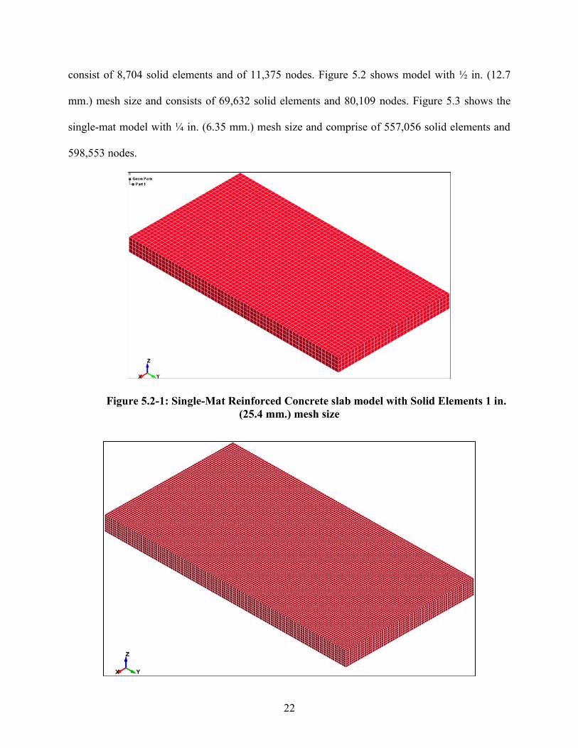
consist of 8,704 solid elements and of 11,375 nodes. Figure 5.2 shows model with ½ in. (12.7
mm.) mesh size and consists of 69,632 solid elements and 80,109 nodes. Figure 5.3 shows the
single-mat model with ¼ in. (6.35 mm.) mesh size and comprise of 557,056 solid elements and
598,553 nodes.
Figure 5.2-1: Single-Mat Reinforced Concrete slab model with Solid Elements 1 in.
(25.4 mm.) mesh size
23
Figure 5.2-2: Single-Mat Reinforced Concrete slab model with Solid Elements ½ in.
(12.7 mm.) mesh size
Figure 5.2-3: Single-Mat Reinforced Concrete slab model with Solid Elements ¼ in.
(6.35 mm.) mesh size
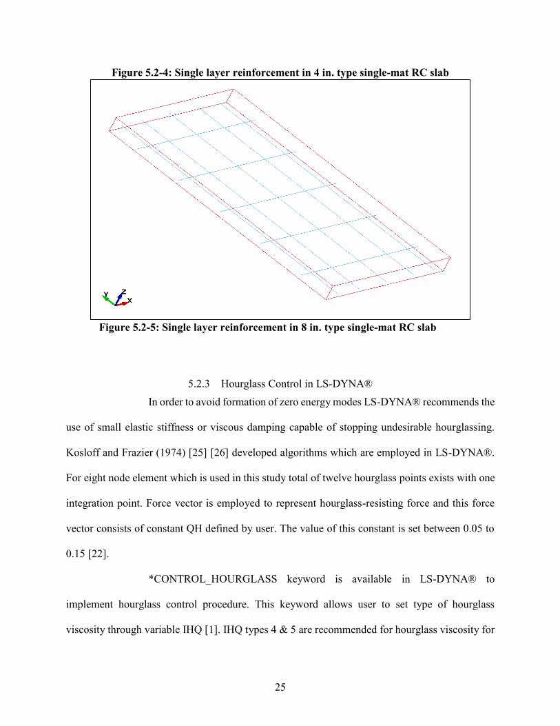
5.2.2 Meshing for Steel Model
From 1 in. (25.4 mm.) concrete cover from back face of concrete slab has single
layer steel reinforcement hence this model is Single-Mat RC slab. Hughes-Liu Beam elements are
used to model steel reinforcements. These elements are employed with cross-section integrations
formulation and has three different mesh sizes like concrete element described before. Two
different main steel spacing 4 in. (101.6 mm.) and 8 in. (203.2 mm.) are used. For 4 in. (101.6
mm.) main steel spacing slabs have two end bars at 2 in. (50.8 mm.) spacing and shrinkage steel
modeled at 12 in. (304.8 mm.) spacing on center. Similarly, for 8 in. (203.2 mm.) main steel
spacing slabs have the two end bars at 6 in. (152.4 mm.) spacing and shrinkage steel modeled at
12 in. (304.8 mm.) spacing on centers. For 4 in. type model with 1 in. (25.4 mm) mesh size models
contain 746 beam elements. Similarly, for ½ in. (12.7 mm.) mesh size consists of 1492 beam
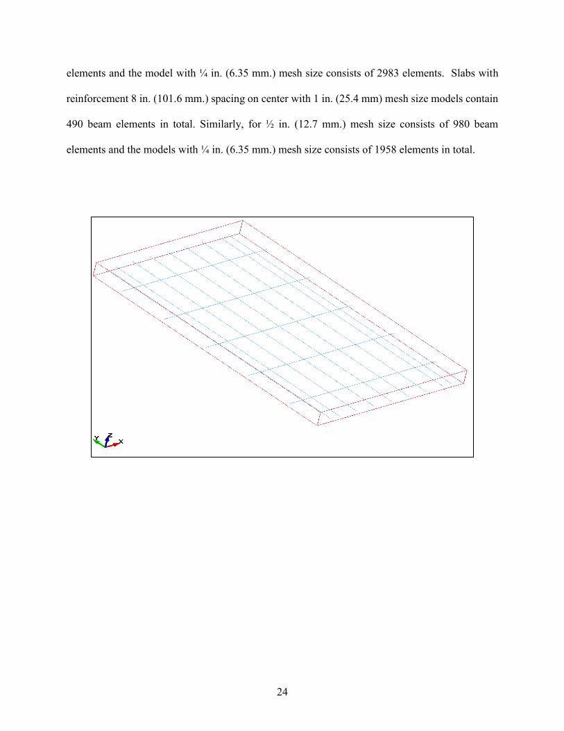
24
elements and the model with ¼ in. (6.35 mm.) mesh size consists of 2983 elements. Slabs with
reinforcement 8 in. (101.6 mm.) spacing on center with 1 in. (25.4 mm) mesh size models contain
490 beam elements in total. Similarly, for ½ in. (12.7 mm.) mesh size consists of 980 beam
elements and the models with ¼ in. (6.35 mm.) mesh size consists of 1958 elements in total.
25
Figure 5.2-4: Single layer reinforcement in 4 in. type single-mat RC slab
Figure 5.2-5: Single layer reinforcement in 8 in. type single-mat RC slab
5.2.3 Hourglass Control in LS-DYNA®
In order to avoid formation of zero energy modes LS-DYNA® recommends the
use of small elastic stiffness or viscous damping capable of stopping undesirable hourglassing.
Kosloff and Frazier (1974) [25] [26] developed algorithms which are employed in LS-DYNA®.
For eight node element which is used in this study total of twelve hourglass points exists with one
integration point. Force vector is employed to represent hourglass-resisting force and this force
vector consists of constant QH defined by user. The value of this constant is set between 0.05 to
0.15 [22].
*CONTROL_HOURGLASS keyword is available in LS-DYNA® to
implement hourglass control procedure. This keyword allows user to set type of hourglass
viscosity through variable IHQ [1]. IHQ types 4 & 5 are recommended for hourglass viscosity for
26
stiffness type control. Hourglass co-efficient is set in *CONTROL_HOURGLASS keyword
through variable QH [1]. This user defined value should be kept less than 1.5, as value exceeding
1.5 may lead to instability. Use of hourglass resistance may lead to loss of energy as work done
by resistance of hourglass is neglected in energy equation. Hence, to validate the accuracy of
simulation total energy of system throughout simulation must by analyzed which consist of friction
energy, damping energy, internal energy, kinetic energy and hourglass energy. In internal energy
includes work done in plastic deformations and elastic strain energy. Output files of MATSUM
and GLSTAT consists data of energy loss due to dissipation of energy by hourglass forces reacting
against formation of hourglass modes. For computation of hourglass energy and inclusion in
energy balance is done under *CONTROL_ENERGY keyword variable HGEN by selection of
type 2 [1]. In order to hourglass control work effectively, non-physical hourglass energy should
be small relative to the peak internal energy (< 10% as rule of thumb) [23].
5.2.4 The Constrained Lagrange in Solid formulation
*CONSTRAINED_LAGRANGE_IN_SOLID (CLS) keyword is used to define
the interface between steel and concrete. This interface is assumed to be a perfect bond. In this
formulation of steel and concrete element nodes are independent of each other. Vasudevan [21]
performed a study on CLS using the Double-mat Reinforced Concrete slab for two concrete
material models Winfrith Concrete Model and Concrete Damage Model Release 3. Shetye [2]
studied effects of CLS formulation for Single-mat model with same concrete material model used
by Vasudevan and compared the both numerical results and experimental.
5.2.5 The Constrained Beam in Solid formulation
Keyword *CONSTRAIN_BEAM_IN_SOLID is alternative to
*CONSTRAIN_LAGRANGE_IN_SOLID and its purpose is to sidestep certain limitations on the
27
CTYPE = 2 in *CONSTRAIN_LAGRANGE_IN_SOLID. *CONSTRAIN_BEAM_IN_SOLID
constrains beam structures to move the Lagrangian solid/thick shell, which are employed as master
components, as it also assumes perfect bond between steel and concrete.
The advantage of *CONSTRAIN_BEAM_IN_SOLID keyword is that the user
can define their own function for bond slip in this keyword using AXFOR input. Function ID is
entered in this input and LS-DYNA manual recommends using AXFOR = -10 were 10 is the
function the ID [1]. Alternatively, program can generate its own bond slip function if user does
not use their own function and parameter CDIR = 0 should be entered for this purpose. In this
study both program generated function and three user-defined functions are compared for all slabs.
For employing a user defined function in this keyword input CDIR = 1 is recommended [1].
NCOUP feature can be used for coupling multiple points in between the beam elements nodes.
This thesis also studies this parameter’s effect on all slip functions used. The following sections
discusses three functions defined for slip between steel reinforcement and concrete.
5.2.5.1 CEB-FIP Function
Grassl [3] conducted research using bond-slip to define interaction between
concrete and steel using the equations of the European CEB-FIP Model code [1] and compared it
with perfect bond. A 3D finite element model was developed for this purpose is LS-DYNA using
damage-plasticity constitutive *MAT_CONCRETE_DAMAGE_PLASTIC_MODEL (CDPME)
for concrete [1]. Coincident slip approach is introduced by spring in between nodes of steel and
concrete and tension stiffening effect was reproduced in bond-slip equation. For this purpose, three
orthogonally oriented springs were used to model interaction between steel and concrete. These
three springs inserted between the coincident nodes. One spring is aligned with average axial
direction of two adjacent beam elements and other two springs are in lateral direction to the beam
28
axis. To define bond-slip law following equations are used in this study; first part (s < smax) is
identical to CEB-FIP model requirements, second part (s ≥ 𝑠𝑚𝑎𝑥) considers Tmax remains constant
after max slip is reached.
𝑇𝑏 = {
𝑇𝑚𝑎𝑥 (𝑠
𝑠𝑚𝑎𝑥)
0.4
if s < 𝑠𝑚𝑎𝑥
𝑇𝑚𝑎𝑥 if s ≥ 𝑠𝑚𝑎𝑥
The first part of bond-slip function (s < 𝑠𝑚𝑎𝑥) is INDE to CEB-FIP Model,
𝑠𝑚𝑎𝑥 is the slip at which bond value is reached and 𝑇𝑚𝑎𝑥 = 2√𝑓𝑐′ MPa. Hence, for high strength
concrete 15 ksi (103.42 MPa) concrete, 𝑇𝑚𝑎𝑥 = 2√103.42 = 20.27 MPa (2940 psi) and for
normal strength concrete 5 ksi (34.47 MPa), 𝑇𝑚𝑎𝑥 = 2√34.47 = 11.60 MPa (1700psi.).
5.2.5.2 CEB-FIP-S3 Function
A study conducted by Grassl [3] studied peak deflection and the residual
deflection was neglected. Hence, the second part of bond-slip function (s ≥ 𝑠𝑚𝑎𝑥) Tmax value
remains constant. In order to properly define residual deflection a new parameter (S3) is
introduced. The new function is defined as follows;
𝑇𝑏 = {
𝑇𝑚𝑎𝑥 (𝑠
𝑠𝑚𝑎𝑥)
0.4
if s < 𝑠𝑚𝑎𝑥
𝑇𝑚𝑎𝑥
𝑆3−𝑠𝑚𝑎𝑥 (S3-𝑠max ) if 𝑠𝑚𝑎𝑥 < 𝑠 < S3
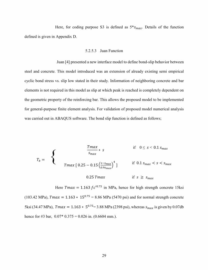
29
Here, for coding purpose S3 is defined as 5*𝑠𝑚𝑎𝑥. Details of the function
defined is given in Appendix D.
5.2.5.3 Juan Function
Juan [4] presented a new interface model to define bond-slip behavior between
steel and concrete. This model introduced was an extension of already existing semi empirical
cyclic bond stress vs. slip low stated in their study. Information of neighboring concrete and bar
elements is not required in this model as slip at which peak is reached is completely dependent on
the geometric property of the reinforcing bar. This allows the proposed model to be implemented
for general-purpose finite element analysis. For validation of proposed model numerical analysis
was carried out in ABAQUS software. The bond slip function is defined as follows;
𝑇𝑏 = {
𝑇𝑚𝑎𝑥
𝑠𝑚𝑎𝑥∗ 𝑠
if 0 ≤ 𝑠 < 0.1 𝑠𝑚𝑎𝑥
𝑇𝑚𝑎𝑥 [ 0.25 − 0.15 (𝑠−𝑠𝑚𝑎𝑥
0.9𝑠𝑚𝑎𝑥)
4
] if 0.1 𝑠𝑚𝑎𝑥 < 𝑠 < 𝑠𝑚𝑎𝑥
0.25 𝑇𝑚𝑎𝑥 if 𝑠 ≥ 𝑠𝑚𝑎𝑥
Here 𝑇𝑚𝑎𝑥 = 1.163 𝑓𝑐′0.75 in MPa, hence for high strength concrete 15ksi
(103.42 MPa), 𝑇𝑚𝑎𝑥 = 1.163 ∗ 150.75 = 8.86 MPa (5470 psi) and for normal strength concrete
5ksi (34.47 MPa), 𝑇𝑚𝑎𝑥 = 1.163 ∗ 50.75= 3.88 MPa (2398 psi), whereas 𝑠𝑚𝑎𝑥 is given by 0.07db
hence for #3 bar, 0.07* 0.375 = 0.026 in. (0.6604 mm.).
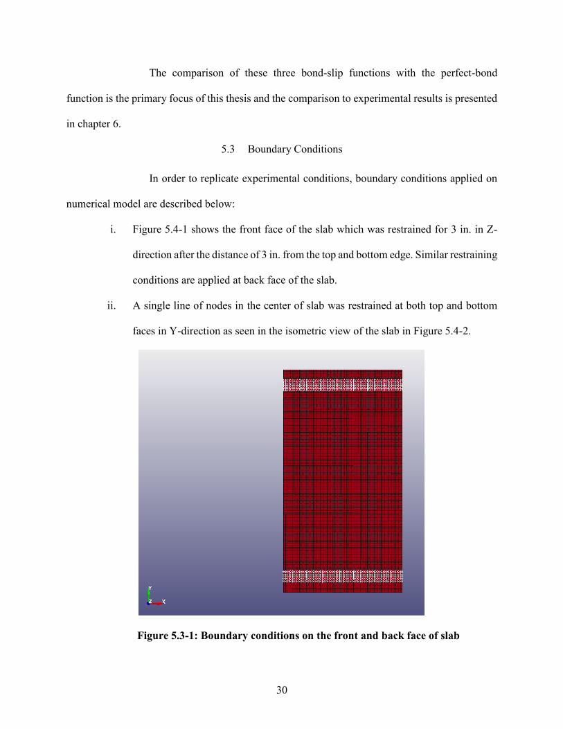
30
The comparison of these three bond-slip functions with the perfect-bond
function is the primary focus of this thesis and the comparison to experimental results is presented
in chapter 6.
5.3 Boundary Conditions
In order to replicate experimental conditions, boundary conditions applied on
numerical model are described below:
i. Figure 5.4-1 shows the front face of the slab which was restrained for 3 in. in Z-
direction after the distance of 3 in. from the top and bottom edge. Similar restraining
conditions are applied at back face of the slab.
ii. A single line of nodes in the center of slab was restrained at both top and bottom
faces in Y-direction as seen in the isometric view of the slab in Figure 5.4-2.
Figure 5.3-1: Boundary conditions on the front and back face of slab
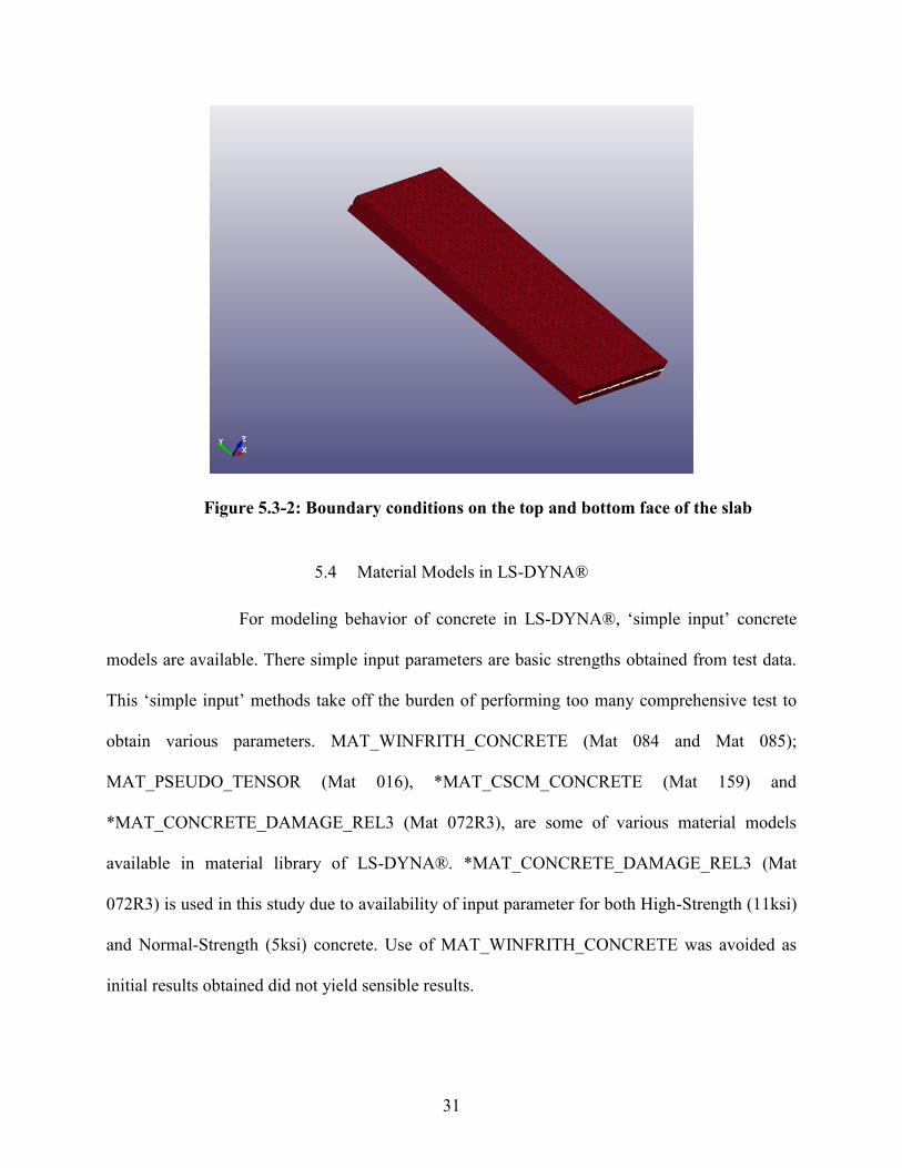
31
Figure 5.3-2: Boundary conditions on the top and bottom face of the slab
5.4 Material Models in LS-DYNA®
For modeling behavior of concrete in LS-DYNA®, ‘simple input’ concrete
models are available. There simple input parameters are basic strengths obtained from test data.
This ‘simple input’ methods take off the burden of performing too many comprehensive test to
obtain various parameters. MAT_WINFRITH_CONCRETE (Mat 084 and Mat 085);
MAT_PSEUDO_TENSOR (Mat 016), *MAT_CSCM_CONCRETE (Mat 159) and
*MAT_CONCRETE_DAMAGE_REL3 (Mat 072R3), are some of various material models
available in material library of LS-DYNA®. *MAT_CONCRETE_DAMAGE_REL3 (Mat
072R3) is used in this study due to availability of input parameter for both High-Strength (11ksi)
and Normal-Strength (5ksi) concrete. Use of MAT_WINFRITH_CONCRETE was avoided as
initial results obtained did not yield sensible results.
32
5.4.1 The Concrete Damage Model Release 3
The Concrete Damage Model Release 3 generates model parameter based on
unconfined compressive strength of concrete and this is its most significant aspect of this material
model. This is done by characterizing most of concrete properties including both plastic and elastic
response critical to blast analysis [30]. Only 1 or 2 parameter input values are required to represent
the complex material concrete and hence termed as a ‘Simple input’ model [14] [28]. Although
internal parameter generation is available, user can also provide their input parameters which is
recommended by Malvar and Schwer in their study [14] if laboratory test data for various
parameters required are available. Once parameters are generated for unconfined compressive
strength of concrete these generated parameters are written and stored in the LS-DYNA® message
file where they can be modified later by the user. Similarly, ‘Tabulated Compaction Equation-of-
state’ (EOS 8) is generated by program for pressure-volume strain response for the model. These
parameters are also written and stored in the “messag” file [1]. These parameters obtained are
studied and modified and again given as input in keyword file. This keyword file with modified
parameters are analyzed using LS-DYNA® manager and LS-PrePost is employed to observe
results.
5.4.1.1 The Three-Shear Failure Surfaces in Concrete Damage Model Release 3
The Karagozian and Case (K&C) – Concrete Damage Model Release 3 uses 3-
shear failure surfaces, initial yield surface residual failure surface and maximum shear failure
surface which makes it a three invariant material model along with incorporating with strain-rate
and damage effects. Set of seven cards of model input parameters are required to be defined for
this material model along with Equation-of-State for the pressure-volume strain response [1].
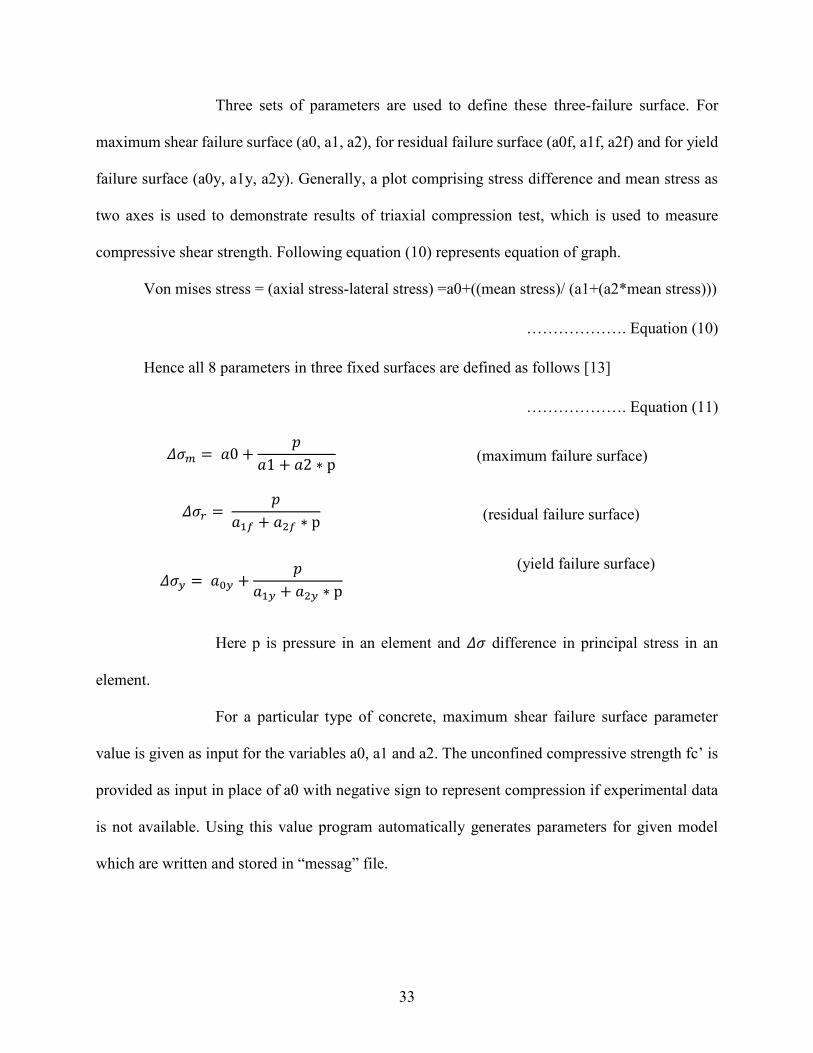
33
Three sets of parameters are used to define these three-failure surface. For
maximum shear failure surface (a0, a1, a2), for residual failure surface (a0f, a1f, a2f) and for yield
failure surface (a0y, a1y, a2y). Generally, a plot comprising stress difference and mean stress as
two axes is used to demonstrate results of triaxial compression test, which is used to measure
compressive shear strength. Following equation (10) represents equation of graph.
Von mises stress = (axial stress-lateral stress) =a0+((mean stress)/ (a1+(a2*mean stress)))
………………. Equation (10)
Hence all 8 parameters in three fixed surfaces are defined as follows [13]
………………. Equation (11)
Here p is pressure in an element and 𝛥𝜎 difference in principal stress in an
element.
For a particular type of concrete, maximum shear failure surface parameter
value is given as input for the variables a0, a1 and a2. The unconfined compressive strength fc’ is
provided as input in place of a0 with negative sign to represent compression if experimental data
is not available. Using this value program automatically generates parameters for given model
which are written and stored in “messag” file.
𝛥𝜎𝑚 = 𝑎0 +𝑝
𝑎1 + 𝑎2 ∗ p (maximum failure surface)
𝛥𝜎𝑟 = 𝑝
𝑎1𝑓 + 𝑎2𝑓 ∗ p (residual failure surface)
𝛥𝜎𝑦 = 𝑎0𝑦 +𝑝
𝑎1𝑦 + 𝑎2𝑦 ∗ p
(yield failure surface)
34
5.4.1.2 The tensile strength of concrete
Based upon unconfined compressive strength input of tensile strength of
concrete can be designated. This is achieved by relationship described below which is based on
CEB-FIP Model Code 1990 as used by Malvar and Schwer [11];
𝑓𝑡 = 1.58 ∗ (𝑓𝑐′2
𝑎0)
13
………………...Equation (12)
According to equation 12 relation tensile strength for unconfined compressive
strength of 11.6 ksi concrete is 7.832 ksi and for 5 ksi unconfined compressive strength, tensile
strength is 4.62 ksi. Some tensile strength values are obtained using automatic parameter
generation method for The Karagozian and Case (K&C) – Concrete Damage Model Release 3
model are written in ‘messag’ file.
5.4.1.3 Equation of State for Concrete Damage Model Release 3
In order to provide pressure and volume strains Concrete Damage Model
release 3 employs an Equation of state. Study conducted by Malvar and Schwer [11] concluded
that in comparison with laboratory data for 46.5 MPa, concrete response of Concrete Damage
Model 3 gives less values in comparison to experimental records. Hence, in order to avoid
variability in volumetric response for concrete (Equation of State), calibration of this material
model is required for specific material. Thus, use of pressure-volume strain data is required for
particular concrete material. The laboratory data available for 11.6 ksi concrete and 5 ksi concrete
is shown in Figure 5.5-1 and 5.5-2 respectively and these values are default parameters are replaced
with these values in ‘messag’ file [2]. The Equation of state thus obtained is provided as new input
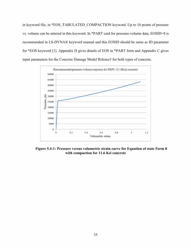
35
in keyword file, in *EOS_TABULATED_COMPACTION keyword. Up to 10 points of pressure
vs. volume can be entered in this keyword. In *PART card for pressure-volume data, EOSID=8 is
recommended in LS-DYNA® keyword manual and this EOSID should be same as ID parameter
for *EOS keyword [1]. Appendix D gives details of EOS in *PART form and Appendix C gives
input parameters for the Concrete Damage Model Release3 for both types of concrete.
Figure 5.4-1: Pressure versus volumetric strain curve for Equation of state Form 8
with compaction for 11.6 Ksi concrete
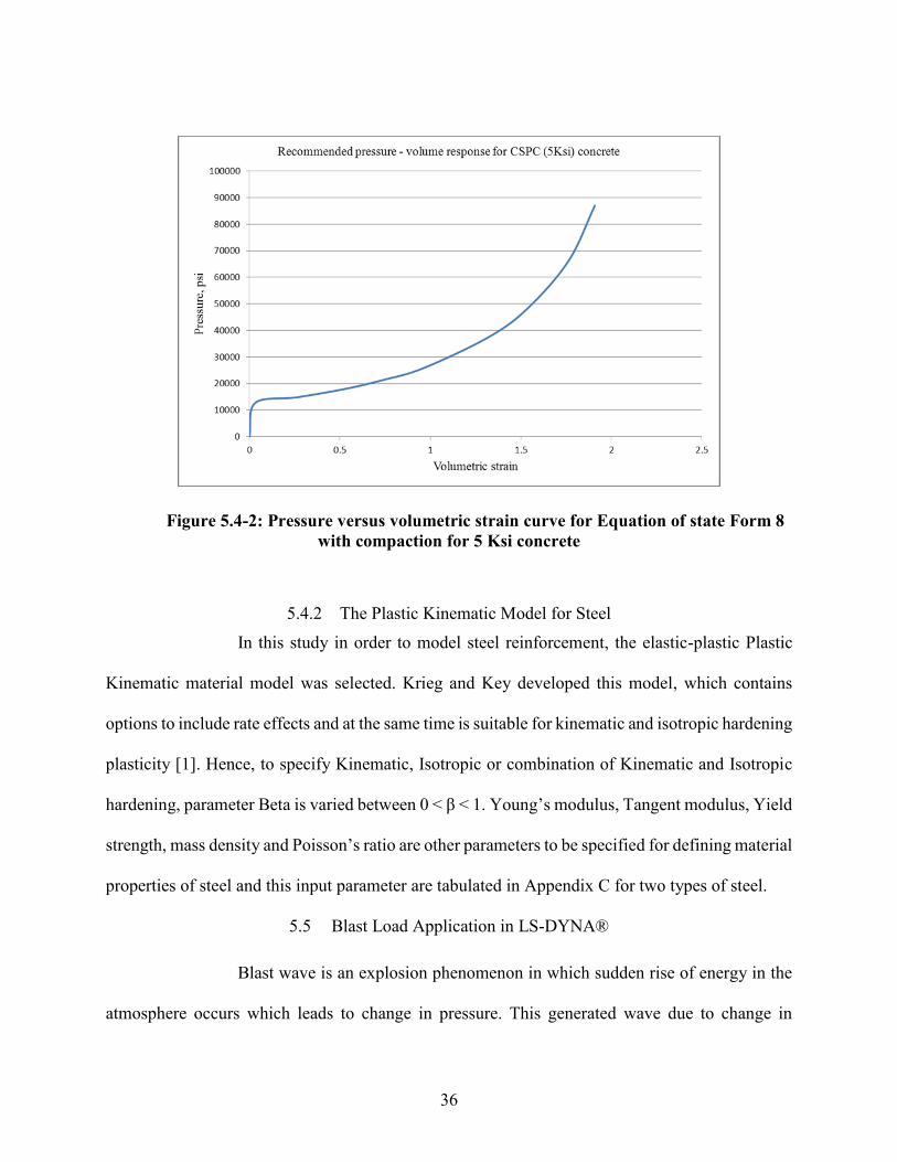
36
Figure 5.4-2: Pressure versus volumetric strain curve for Equation of state Form 8
with compaction for 5 Ksi concrete
5.4.2 The Plastic Kinematic Model for Steel
In this study in order to model steel reinforcement, the elastic-plastic Plastic
Kinematic material model was selected. Krieg and Key developed this model, which contains
options to include rate effects and at the same time is suitable for kinematic and isotropic hardening
plasticity [1]. Hence, to specify Kinematic, Isotropic or combination of Kinematic and Isotropic
hardening, parameter Beta is varied between 0 < β < 1. Young’s modulus, Tangent modulus, Yield
strength, mass density and Poisson’s ratio are other parameters to be specified for defining material
properties of steel and this input parameter are tabulated in Appendix C for two types of steel.
5.5 Blast Load Application in LS-DYNA®
Blast wave is an explosion phenomenon in which sudden rise of energy in the
atmosphere occurs which leads to change in pressure. This generated wave due to change in
37
pressure propagates in all direction emerging form source at very high speed. Nature of explosion
and distance of point of consideration form source of explosion are factors which determine
magnitude and shape of blast wave at desired point.
A shock tube is used to generate pressure which is equivalent to pressure
generated by blast wave. Shock wave facilitates sudden rise in pressure above ambient pressure
which later leads to gradual fall below ambient pressure which results in negative pressure wave.
This can be used to define parameters of blast wave. Peak side-on positive overpressure Pso, with
positive phase duration td and corresponding positive impulse Io are parameter of blast waves to be
used. negative phase of same parameter are denoted by Pso-, td
- and Io- respectively.
In order to define blast wave in an accurate manner it is important to define
these blast wave parameters in finite element analysis which replicates blast phenomenon of shock
tube. To define the load curve and slab surface interaction in LS-DYNA®,
*LOAD_SEGMENT_SET keyword is employed along with *DEFINE_CURVE which is used for
pressure vs. time co-ordinates. Appendix B illustrates pressure versus time history with impulse
values for all 12 slabs whereas figure B-1 to B-12 shows all load curves applied to the front face
of respective slabs.
Thus, using various parameters and keywords of LS-DYNA®, numerical
modeling of 12 reinforced concrete slabs are achieved. All simulation are completed using LS
manager and later LS post processor is used for obtaining results of these simulations. Results
which are important for this thesis, are mid-span deflection time histories for all bond relations
between concrete and steel. Results from numerical simulations are presented in the following
chapter.
38
CHAPTER 6. NUMERICAL ANALUSIS RESULTS AND COMAPRISON WITH
EXPERIMENTAL
In this chapter experimental records are compared with numerical simulation
results obtained from LS-DYNA®. The criterion used for comparison is peak deflection history.
Numerical simulations were performed on twelve slabs of two different material strength, two
separate reinforcement ratios and two types of bond relations are compared in this chapter.
Since Beam in Solid formulation is being investigated in this study, the
parameters of this new keyword are compared, and four slabs consisting of different slab setups
are studied for this purpose. Firstly, the effect of boundary conditions are investigated followed by
a study of the effect of mesh analysis.
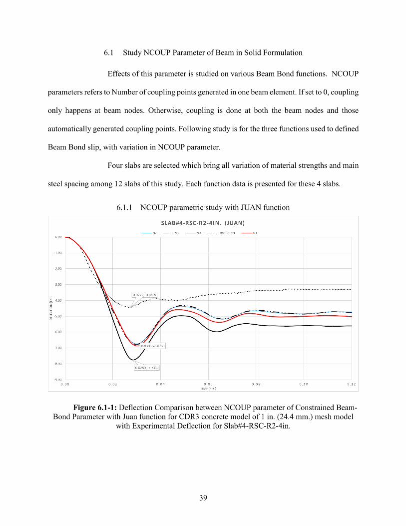
39
6.1 Study NCOUP Parameter of Beam in Solid Formulation
Effects of this parameter is studied on various Beam Bond functions. NCOUP
parameters refers to Number of coupling points generated in one beam element. If set to 0, coupling
only happens at beam nodes. Otherwise, coupling is done at both the beam nodes and those
automatically generated coupling points. Following study is for the three functions used to defined
Beam Bond slip, with variation in NCOUP parameter.
Four slabs are selected which bring all variation of material strengths and main
steel spacing among 12 slabs of this study. Each function data is presented for these 4 slabs.
6.1.1 NCOUP parametric study with JUAN function
Figure 6.1-1: Deflection Comparison between NCOUP parameter of Constrained Beam-
Bond Parameter with Juan function for CDR3 concrete model of 1 in. (24.4 mm.) mesh model
with Experimental Deflection for Slab#4-RSC-R2-4in.
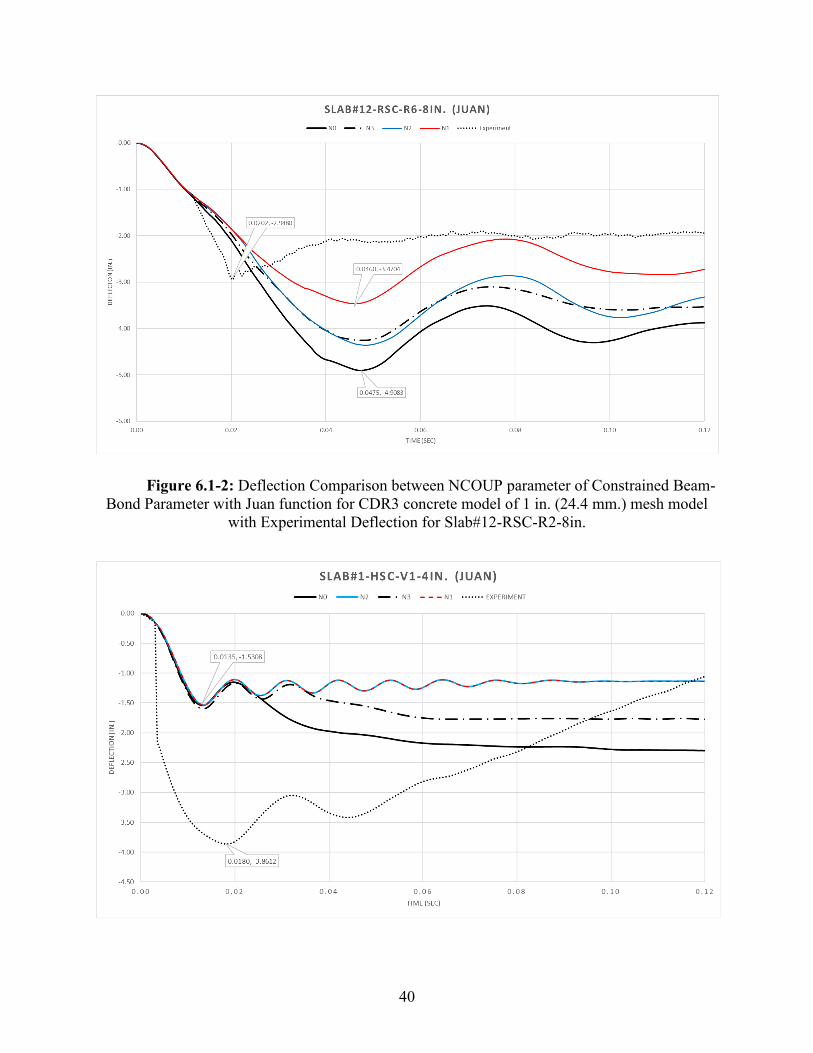
40
Figure 6.1-2: Deflection Comparison between NCOUP parameter of Constrained Beam-
Bond Parameter with Juan function for CDR3 concrete model of 1 in. (24.4 mm.) mesh model
with Experimental Deflection for Slab#12-RSC-R2-8in.
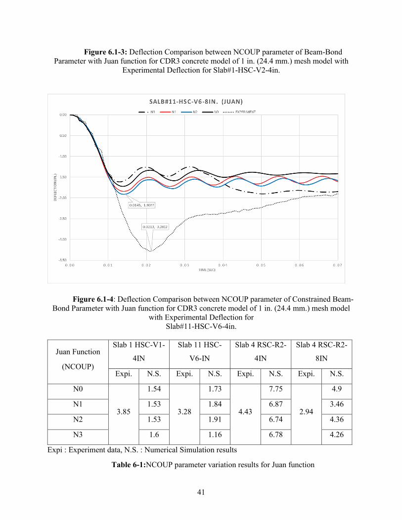
41
Figure 6.1-3: Deflection Comparison between NCOUP parameter of Beam-Bond
Parameter with Juan function for CDR3 concrete model of 1 in. (24.4 mm.) mesh model with
Experimental Deflection for Slab#1-HSC-V2-4in.
Figure 6.1-4: Deflection Comparison between NCOUP parameter of Constrained Beam-
Bond Parameter with Juan function for CDR3 concrete model of 1 in. (24.4 mm.) mesh model
with Experimental Deflection for
Slab#11-HSC-V6-4in.
Juan Function
(NCOUP)
Slab 1 HSC-V1-
4IN
Slab 11 HSC-
V6-IN
Slab 4 RSC-R2-
4IN
Slab 4 RSC-R2-
8IN
Expi. N.S. Expi. N.S. Expi. N.S. Expi. N.S.
N0
3.85
1.54
3.28
1.73
4.43
7.75
2.94
4.9
N1 1.53 1.84 6.87 3.46
N2 1.53 1.91 6.74 4.36
N3 1.6 1.16 6.78 4.26
Expi : Experiment data, N.S. : Numerical Simulation results
Table 6-1:NCOUP parameter variation results for Juan function
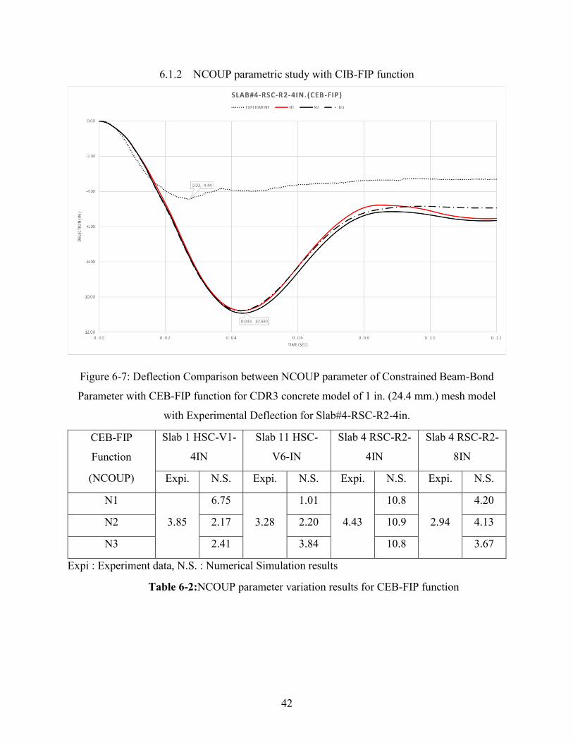
42
6.1.2 NCOUP parametric study with CIB-FIP function
Figure 6-7: Deflection Comparison between NCOUP parameter of Constrained Beam-Bond
Parameter with CEB-FIP function for CDR3 concrete model of 1 in. (24.4 mm.) mesh model
with Experimental Deflection for Slab#4-RSC-R2-4in.
CEB-FIP
Function
(NCOUP)
Slab 1 HSC-V1-
4IN
Slab 11 HSC-
V6-IN
Slab 4 RSC-R2-
4IN
Slab 4 RSC-R2-
8IN
Expi. N.S. Expi. N.S. Expi. N.S. Expi. N.S.
N1
3.85
6.75
3.28
1.01
4.43
10.8
2.94
4.20
N2 2.17 2.20 10.9 4.13
N3 2.41 3.84 10.8 3.67
Expi : Experiment data, N.S. : Numerical Simulation results
Table 6-2:NCOUP parameter variation results for CEB-FIP function
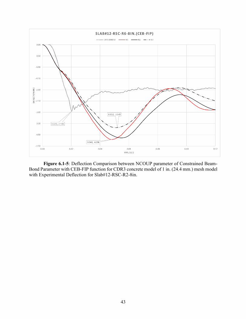
43
Figure 6.1-5: Deflection Comparison between NCOUP parameter of Constrained Beam-
Bond Parameter with CEB-FIP function for CDR3 concrete model of 1 in. (24.4 mm.) mesh model
with Experimental Deflection for Slab#12-RSC-R2-8in.
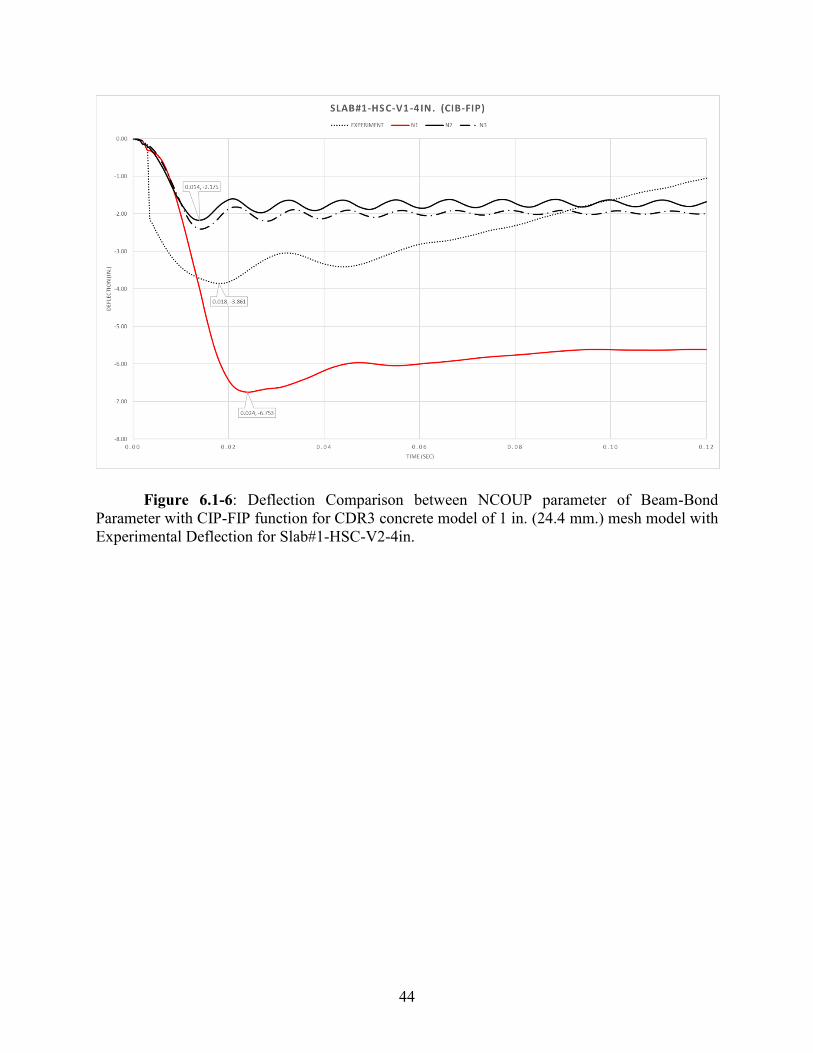
44
Figure 6.1-6: Deflection Comparison between NCOUP parameter of Beam-Bond
Parameter with CIP-FIP function for CDR3 concrete model of 1 in. (24.4 mm.) mesh model with
Experimental Deflection for Slab#1-HSC-V2-4in.
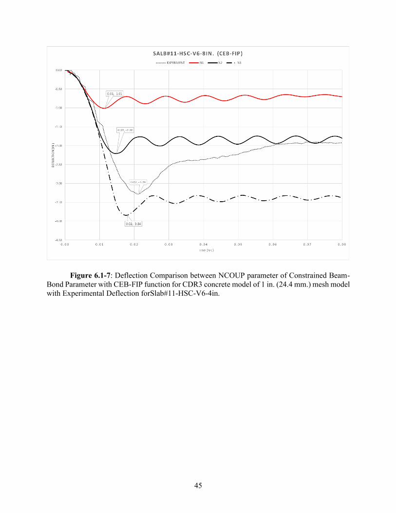
45
Figure 6.1-7: Deflection Comparison between NCOUP parameter of Constrained Beam-
Bond Parameter with CEB-FIP function for CDR3 concrete model of 1 in. (24.4 mm.) mesh model
with Experimental Deflection forSlab#11-HSC-V6-4in.
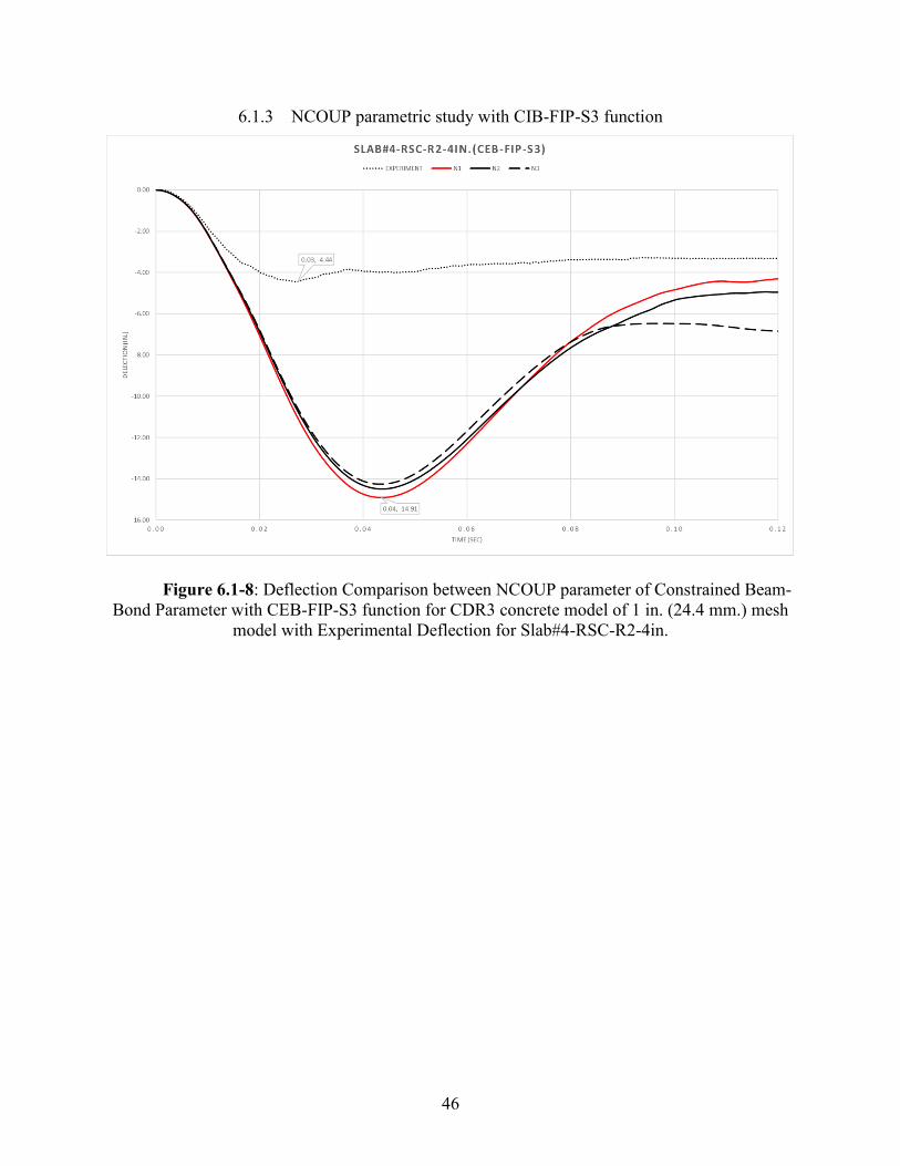
46
6.1.3 NCOUP parametric study with CIB-FIP-S3 function
Figure 6.1-8: Deflection Comparison between NCOUP parameter of Constrained Beam-
Bond Parameter with CEB-FIP-S3 function for CDR3 concrete model of 1 in. (24.4 mm.) mesh
model with Experimental Deflection for Slab#4-RSC-R2-4in.
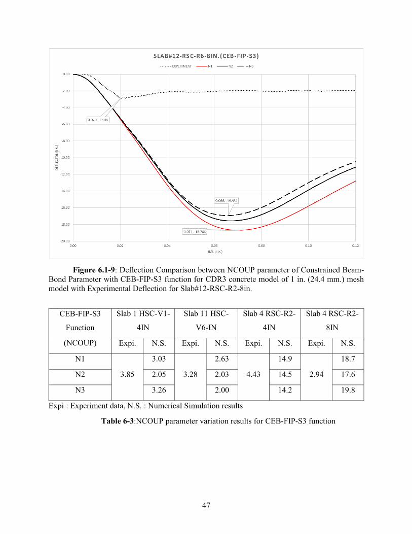
47
Figure 6.1-9: Deflection Comparison between NCOUP parameter of Constrained Beam-
Bond Parameter with CEB-FIP-S3 function for CDR3 concrete model of 1 in. (24.4 mm.) mesh
model with Experimental Deflection for Slab#12-RSC-R2-8in.
CEB-FIP-S3
Function
(NCOUP)
Slab 1 HSC-V1-
4IN
Slab 11 HSC-
V6-IN
Slab 4 RSC-R2-
4IN
Slab 4 RSC-R2-
8IN
Expi. N.S. Expi. N.S. Expi. N.S. Expi. N.S.
N1
3.85
3.03
3.28
2.63
4.43
14.9
2.94
18.7
N2 2.05 2.03 14.5 17.6
N3 3.26 2.00 14.2 19.8
Expi : Experiment data, N.S. : Numerical Simulation results
Table 6-3:NCOUP parameter variation results for CEB-FIP-S3 function
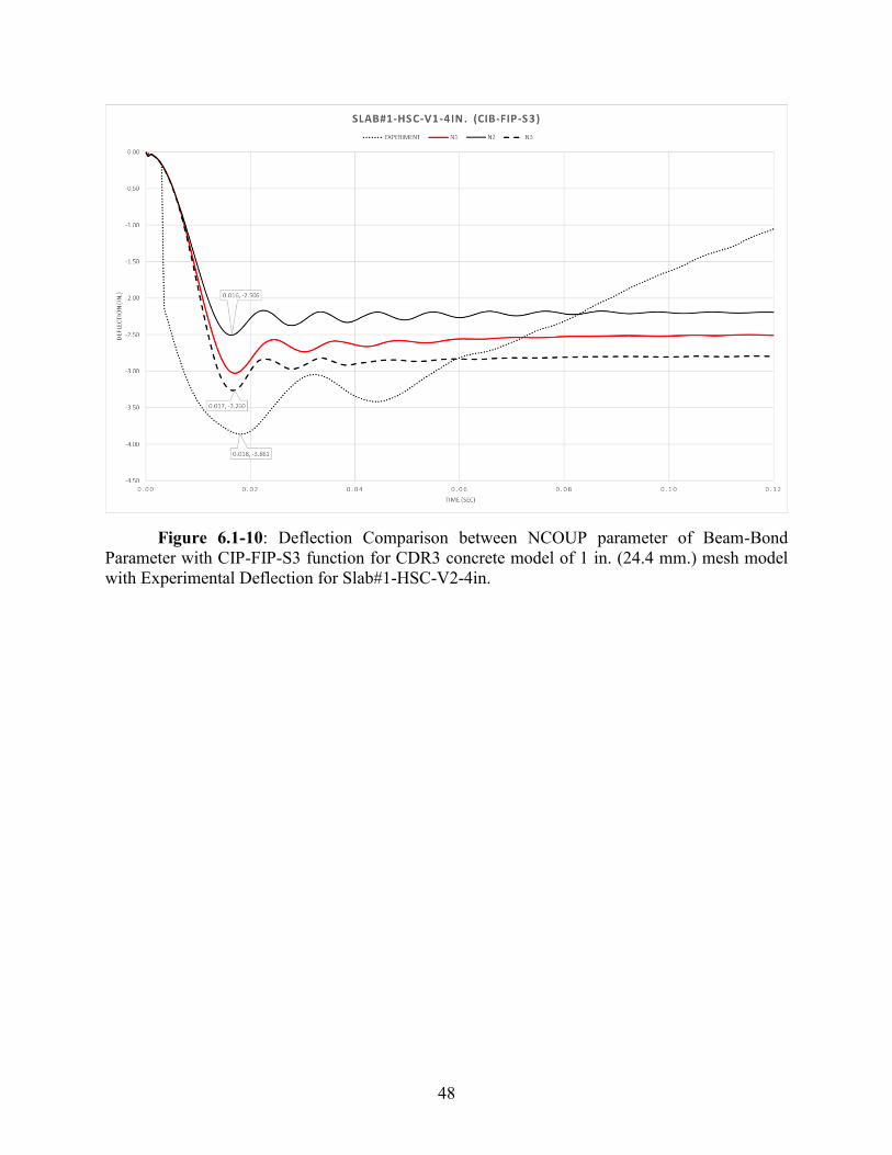
48
Figure 6.1-10: Deflection Comparison between NCOUP parameter of Beam-Bond
Parameter with CIP-FIP-S3 function for CDR3 concrete model of 1 in. (24.4 mm.) mesh model
with Experimental Deflection for Slab#1-HSC-V2-4in.
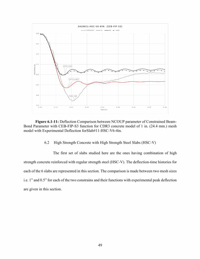
49
Figure 6.1-11: Deflection Comparison between NCOUP parameter of Constrained Beam-
Bond Parameter with CEB-FIP-S3 function for CDR3 concrete model of 1 in. (24.4 mm.) mesh
model with Experimental Deflection forSlab#11-HSC-V6-4in.
6.2 High Strength Concrete with High Strength Steel Slabs (HSC-V)
The first set of slabs studied here are the ones having combination of high
strength concrete reinforced with regular strength steel (HSC-V). The deflection-time histories for
each of the 6 slabs are represented in this section. The comparison is made between two mesh sizes
i.e. 1” and 0.5” for each of the two constrains and their functions with experimental peak deflection
are given in this section.
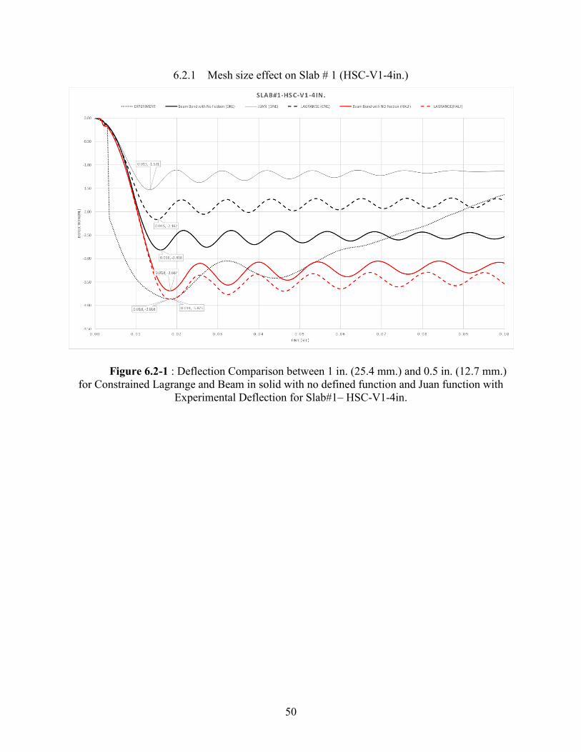
50
6.2.1 Mesh size effect on Slab # 1 (HSC-V1-4in.)
Figure 6.2-1 : Deflection Comparison between 1 in. (25.4 mm.) and 0.5 in. (12.7 mm.)
for Constrained Lagrange and Beam in solid with no defined function and Juan function with
Experimental Deflection for Slab#1– HSC-V1-4in.
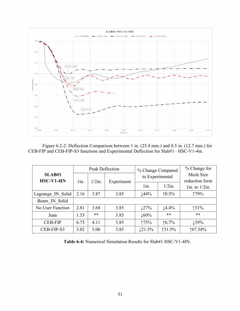
51
Figure 6.2-2: Deflection Comparison between 1 in. (25.4 mm.) and 0.5 in. (12.7 mm.) for
CEB-FIP and CEB-FIP-S3 functions and Experimental Deflection for Slab#1– HSC-V1-4in.
SLAB#1
HSC-V1-4IN
Peak Deflection % Change Compared
to Experimental
% Change for
Mesh Size
reduction form
1in. to 1/2in.
1in. 1/2in. Experiment 1in. 1/2in.
Lagrange_IN_Solid 2.16 3.87 3.85 ↓44% ↑0.5% ↑79%
Beam_IN_Solid
No User Function 2.81 3.68 3.85 ↓27% ↓4.4% ↑31%
Juan 1.53 ** 3.85 ↓60% ** **
CEB-FIP 6.75 4.11 3.85 ↑75% ↑6.7% ↓39%
CEB-FIP-S3 3.02 5.06 3.85 ↓21.5% ↑31.5% ↑67.54%
Table 6-4: Numerical Simulation Results for Slab#1 HSC-V1-4IN.
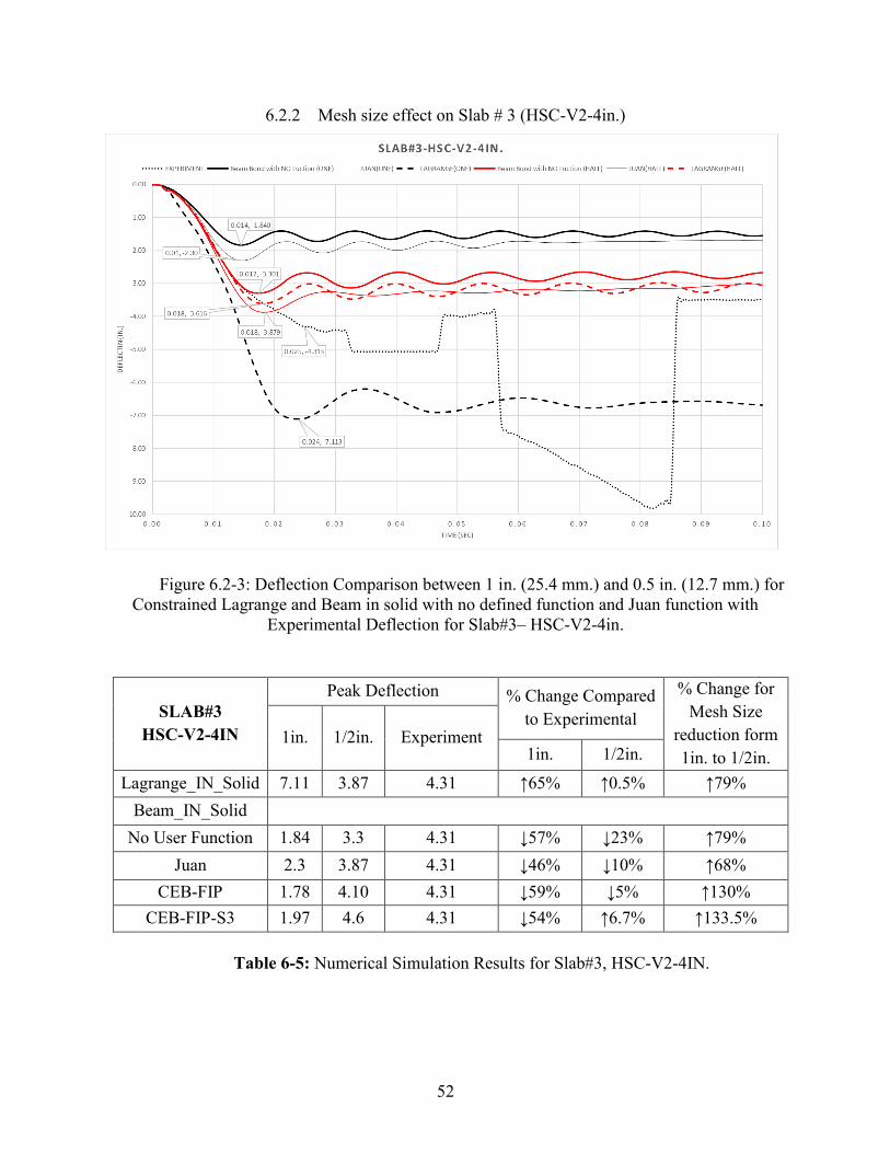
52
6.2.2 Mesh size effect on Slab # 3 (HSC-V2-4in.)
Figure 6.2-3: Deflection Comparison between 1 in. (25.4 mm.) and 0.5 in. (12.7 mm.) for
Constrained Lagrange and Beam in solid with no defined function and Juan function with
Experimental Deflection for Slab#3– HSC-V2-4in.
SLAB#3
HSC-V2-4IN
Peak Deflection % Change Compared
to Experimental
% Change for
Mesh Size
reduction form
1in. to 1/2in.
1in. 1/2in. Experiment 1in. 1/2in.
Lagrange_IN_Solid 7.11 3.87 4.31 ↑65% ↑0.5% ↑79%
Beam_IN_Solid
No User Function 1.84 3.3 4.31 ↓57% ↓23% ↑79%
Juan 2.3 3.87 4.31 ↓46% ↓10% ↑68%
CEB-FIP 1.78 4.10 4.31 ↓59% ↓5% ↑130%
CEB-FIP-S3 1.97 4.6 4.31 ↓54% ↑6.7% ↑133.5%
Table 6-5: Numerical Simulation Results for Slab#3, HSC-V2-4IN.
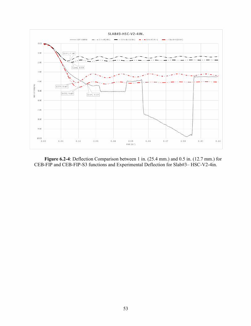
53
Figure 6.2-4: Deflection Comparison between 1 in. (25.4 mm.) and 0.5 in. (12.7 mm.) for
CEB-FIP and CEB-FIP-S3 functions and Experimental Deflection for Slab#3– HSC-V2-4in.
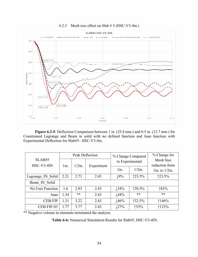
54
6.2.3 Mesh size effect on Slab # 5 (HSC-V3-4in.)
Figure 6.2-5: Deflection Comparison between 1 in. (25.4 mm.) and 0.5 in. (12.7 mm.) for
Constrained Lagrange and Beam in solid with no defined function and Juan function with
Experimental Deflection for Slab#5– HSC-V3-4in.
SLAB#5
HSC-V3-4IN
Peak Deflection % Change Compared
to Experimental
% Change for
Mesh Size
reduction form
1in. to 1/2in.
1in. 1/2in. Experiment 1in. 1/2in.
Lagrange_IN_Solid 2.21 2.73 2.43 ↓9% ↑23.5% ↑23.5%
Beam_IN_Solid
No User Function 1.6 2.93 2.43 ↓34% ↑20.5% ↑83%
Juan 1.34 ** 2.43 ↓44% ** **
CEB-FIP 1.31 3.22 2.43 ↓46% ↑32.5% ↑146%
CEB-FIP-S3 1.77 3.77 2.43 ↓27% ↑55% ↑123%
** Negative volume in elements terminated the analysis
Table 6-6: Numerical Simulation Results for Slab#5, HSC-V3-4IN.
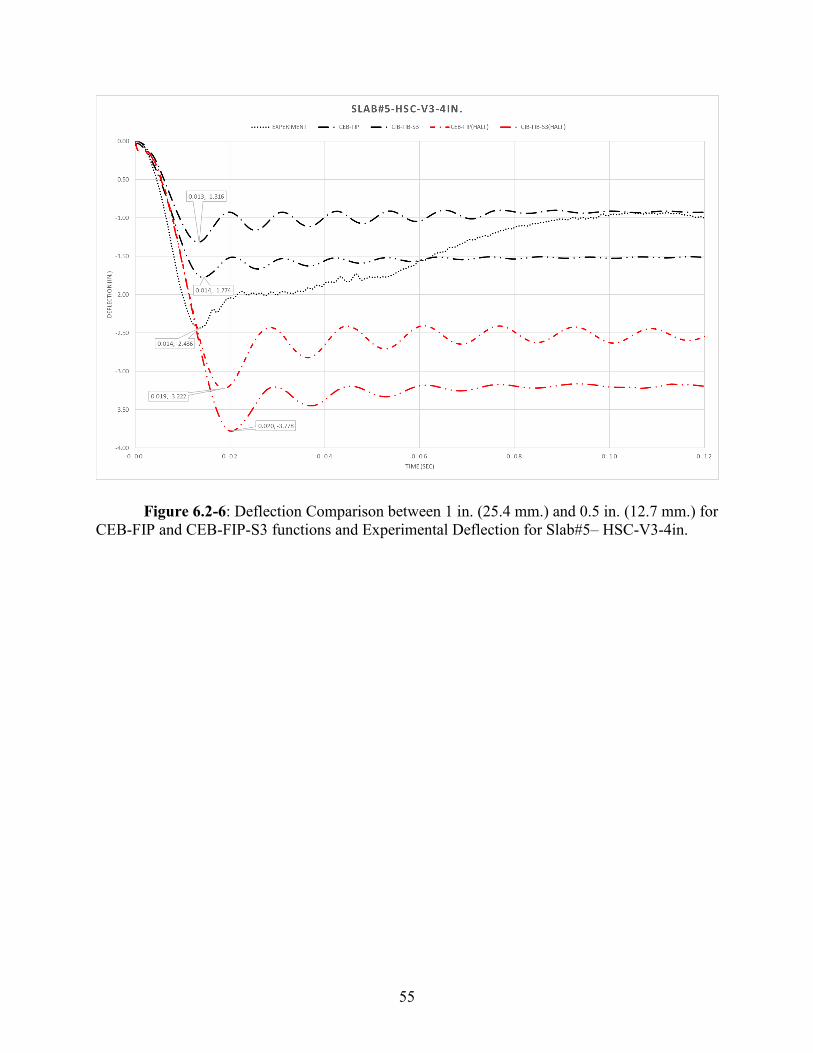
55
Figure 6.2-6: Deflection Comparison between 1 in. (25.4 mm.) and 0.5 in. (12.7 mm.) for
CEB-FIP and CEB-FIP-S3 functions and Experimental Deflection for Slab#5– HSC-V3-4in.
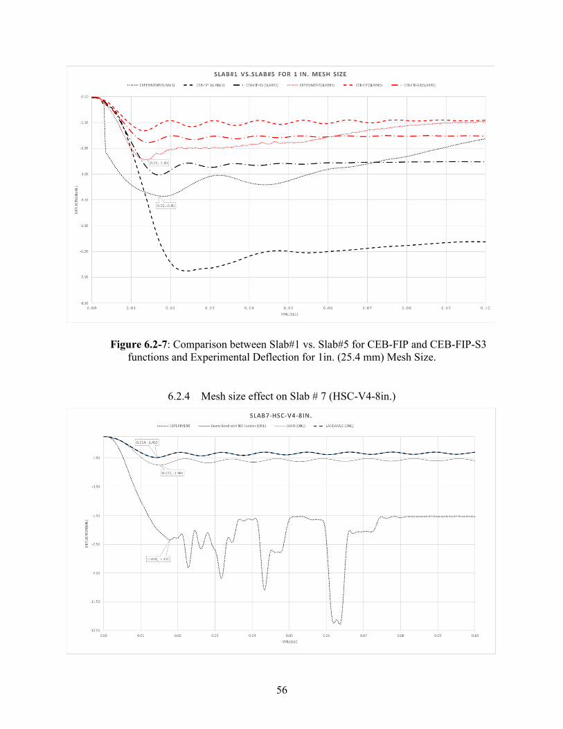
56
Figure 6.2-7: Comparison between Slab#1 vs. Slab#5 for CEB-FIP and CEB-FIP-S3
functions and Experimental Deflection for 1in. (25.4 mm) Mesh Size.
6.2.4 Mesh size effect on Slab # 7 (HSC-V4-8in.)
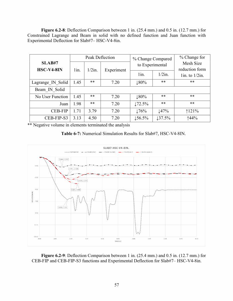
57
Figure 6.2-8: Deflection Comparison between 1 in. (25.4 mm.) and 0.5 in. (12.7 mm.) for
Constrained Lagrange and Beam in solid with no defined function and Juan function with
Experimental Deflection for Slab#7– HSC-V4-8in.
SLAB#7
HSC-V4-8IN
Peak Deflection % Change Compared
to Experimental
% Change for
Mesh Size
reduction form
1in. to 1/2in.
1in. 1/2in. Experiment 1in. 1/2in.
Lagrange_IN_Solid 1.45 ** 7.20 ↓80% ** **
Beam_IN_Solid
No User Function 1.45 ** 7.20 ↓80% ** **
Juan 1.98 ** 7.20 ↓72.5% ** **
CEB-FIP 1.71 3.79 7.20 ↓76% ↓47% ↑121%
CEB-FIP-S3 3.13 4.50 7.20 ↓56.5% ↓37.5% ↑44%
** Negative volume in elements terminated the analysis
Table 6-7: Numerical Simulation Results for Slab#7, HSC-V4-8IN.
Figure 6.2-9: Deflection Comparison between 1 in. (25.4 mm.) and 0.5 in. (12.7 mm.) for
CEB-FIP and CEB-FIP-S3 functions and Experimental Deflection for Slab#7– HSC-V4-8in.
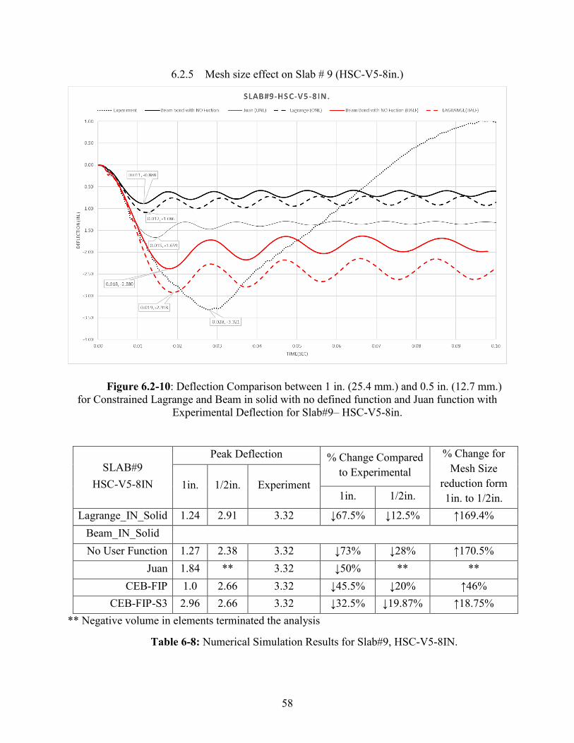
58
6.2.5 Mesh size effect on Slab # 9 (HSC-V5-8in.)
Figure 6.2-10: Deflection Comparison between 1 in. (25.4 mm.) and 0.5 in. (12.7 mm.)
for Constrained Lagrange and Beam in solid with no defined function and Juan function with
Experimental Deflection for Slab#9– HSC-V5-8in.
SLAB#9
HSC-V5-8IN
Peak Deflection % Change Compared
to Experimental
% Change for
Mesh Size
reduction form
1in. to 1/2in.
1in. 1/2in. Experiment 1in. 1/2in.
Lagrange_IN_Solid 1.24 2.91 3.32 ↓67.5% ↓12.5% ↑169.4%
Beam_IN_Solid
No User Function 1.27 2.38 3.32 ↓73% ↓28% ↑170.5%
Juan 1.84 ** 3.32 ↓50% ** **
CEB-FIP 1.0 2.66 3.32 ↓45.5% ↓20% ↑46%
CEB-FIP-S3 2.96 2.66 3.32 ↓32.5% ↓19.87% ↑18.75%
** Negative volume in elements terminated the analysis
Table 6-8: Numerical Simulation Results for Slab#9, HSC-V5-8IN.
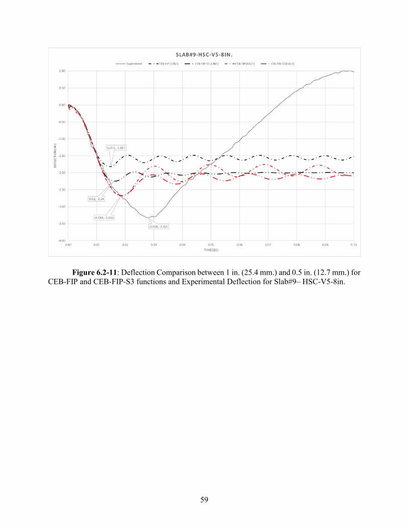
59
Figure 6.2-11: Deflection Comparison between 1 in. (25.4 mm.) and 0.5 in. (12.7 mm.) for
CEB-FIP and CEB-FIP-S3 functions and Experimental Deflection for Slab#9– HSC-V5-8in.
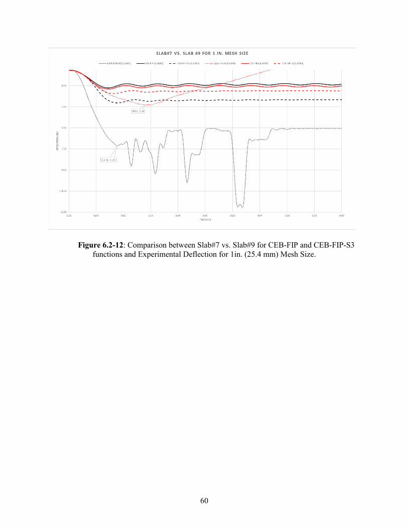
60
Figure 6.2-12: Comparison between Slab#7 vs. Slab#9 for CEB-FIP and CEB-FIP-S3
functions and Experimental Deflection for 1in. (25.4 mm) Mesh Size.
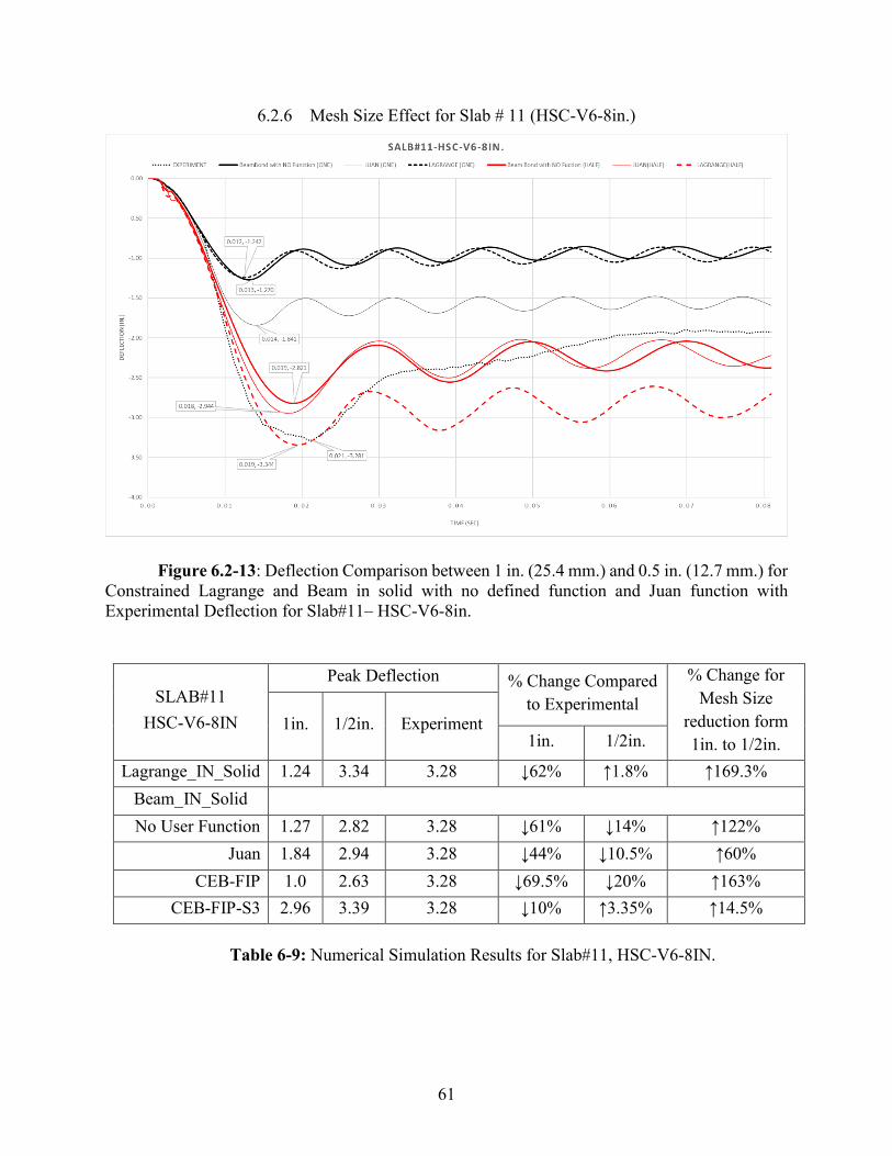
61
6.2.6 Mesh Size Effect for Slab # 11 (HSC-V6-8in.)
Figure 6.2-13: Deflection Comparison between 1 in. (25.4 mm.) and 0.5 in. (12.7 mm.) for
Constrained Lagrange and Beam in solid with no defined function and Juan function with
Experimental Deflection for Slab#11– HSC-V6-8in.
SLAB#11
HSC-V6-8IN
Peak Deflection % Change Compared
to Experimental
% Change for
Mesh Size
reduction form
1in. to 1/2in.
1in. 1/2in. Experiment 1in. 1/2in.
Lagrange_IN_Solid 1.24 3.34 3.28 ↓62% ↑1.8% ↑169.3%
Beam_IN_Solid
No User Function 1.27 2.82 3.28 ↓61% ↓14% ↑122%
Juan 1.84 2.94 3.28 ↓44% ↓10.5% ↑60%
CEB-FIP 1.0 2.63 3.28 ↓69.5% ↓20% ↑163%
CEB-FIP-S3 2.96 3.39 3.28 ↓10% ↑3.35% ↑14.5%
Table 6-9: Numerical Simulation Results for Slab#11, HSC-V6-8IN.
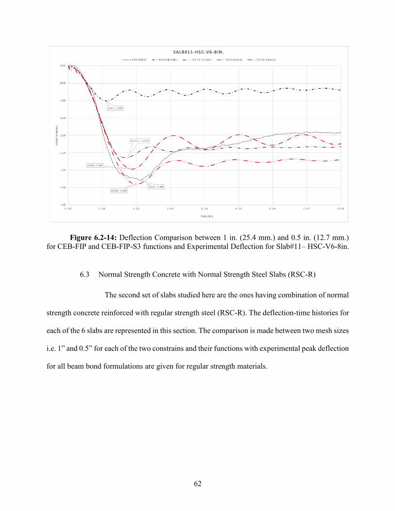
62
Figure 6.2-14: Deflection Comparison between 1 in. (25.4 mm.) and 0.5 in. (12.7 mm.)
for CEB-FIP and CEB-FIP-S3 functions and Experimental Deflection for Slab#11– HSC-V6-8in.
6.3 Normal Strength Concrete with Normal Strength Steel Slabs (RSC-R)
The second set of slabs studied here are the ones having combination of normal
strength concrete reinforced with regular strength steel (RSC-R). The deflection-time histories for
each of the 6 slabs are represented in this section. The comparison is made between two mesh sizes
i.e. 1” and 0.5” for each of the two constrains and their functions with experimental peak deflection
for all beam bond formulations are given for regular strength materials.
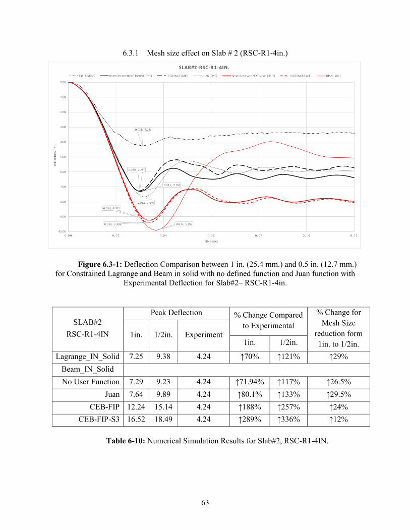
63
6.3.1 Mesh size effect on Slab # 2 (RSC-R1-4in.)
Figure 6.3-1: Deflection Comparison between 1 in. (25.4 mm.) and 0.5 in. (12.7 mm.)
for Constrained Lagrange and Beam in solid with no defined function and Juan function with
Experimental Deflection for Slab#2– RSC-R1-4in.
SLAB#2
RSC-R1-4IN
Peak Deflection % Change Compared
to Experimental
% Change for
Mesh Size
reduction form
1in. to 1/2in.
1in. 1/2in. Experiment 1in. 1/2in.
Lagrange_IN_Solid 7.25 9.38 4.24 ↑70% ↑121% ↑29%
Beam_IN_Solid
No User Function 7.29 9.23 4.24 ↑71.94% ↑117% ↑26.5%
Juan 7.64 9.89 4.24 ↑80.1% ↑133% ↑29.5%
CEB-FIP 12.24 15.14 4.24 ↑188% ↑257% ↑24%
CEB-FIP-S3 16.52 18.49 4.24 ↑289% ↑336% ↑12%
Table 6-10: Numerical Simulation Results for Slab#2, RSC-R1-4IN.
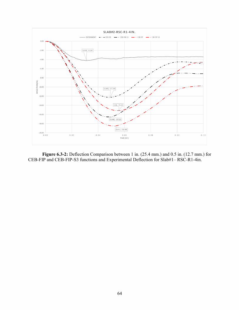
64
Figure 6.3-2: Deflection Comparison between 1 in. (25.4 mm.) and 0.5 in. (12.7 mm.) for
CEB-FIP and CEB-FIP-S3 functions and Experimental Deflection for Slab#1– RSC-R1-4in.
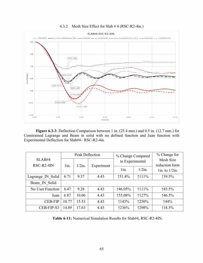
65
6.3.2 Mesh Size Effect for Slab # 4 (RSC-R2-4in.)
Figure 6.3-3: Deflection Comparison between 1 in. (25.4 mm.) and 0.5 in. (12.7 mm.) for
Constrained Lagrange and Beam in solid with no defined function and Juan function with
Experimental Deflection for Slab#4– RSC-R2-4in.
SLAB#4
RSC-R2-4IN
Peak Deflection % Change Compared
to Experimental
% Change for
Mesh Size
reduction form
1in. to 1/2in.
1in. 1/2in. Experiment 1in. 1/2in.
Lagrange_IN_Solid 6.71 9.37 4.43 ↑51.4% ↑111% ↑39.5%
Beam_IN_Solid
No User Function 6.47 9.28 4.43 ↑46.05% ↑111% ↑43.5%
Juan 6.87 10.06 4.43 ↑55.08% ↑127% ↑46.5%
CEB-FIP 10.77 15.53 4.43 ↑143% ↑250% ↑44%
CEB-FIP-S3 14.89 17.63 4.43 ↑236% ↑298% ↑18.5%
Table 6-11: Numerical Simulation Results for Slab#4, RSC-R2-4IN.
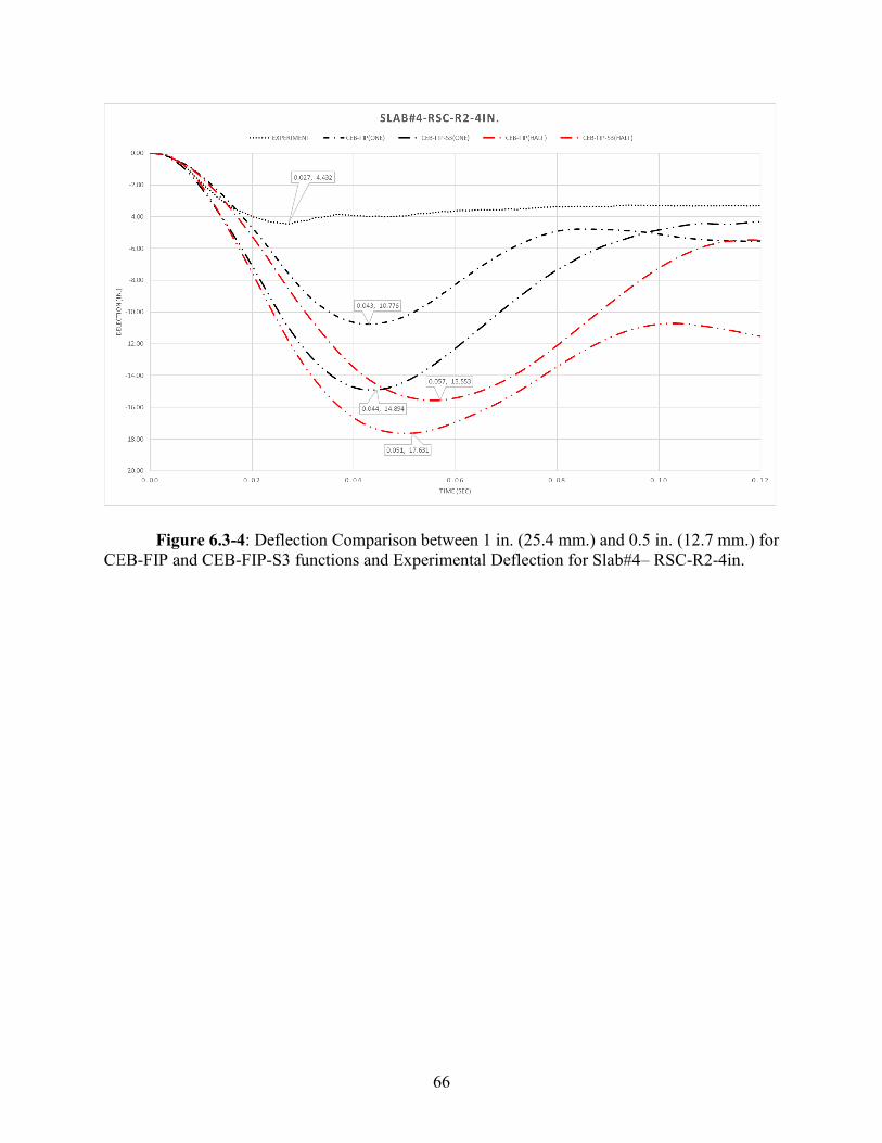
66
Figure 6.3-4: Deflection Comparison between 1 in. (25.4 mm.) and 0.5 in. (12.7 mm.) for
CEB-FIP and CEB-FIP-S3 functions and Experimental Deflection for Slab#4– RSC-R2-4in.
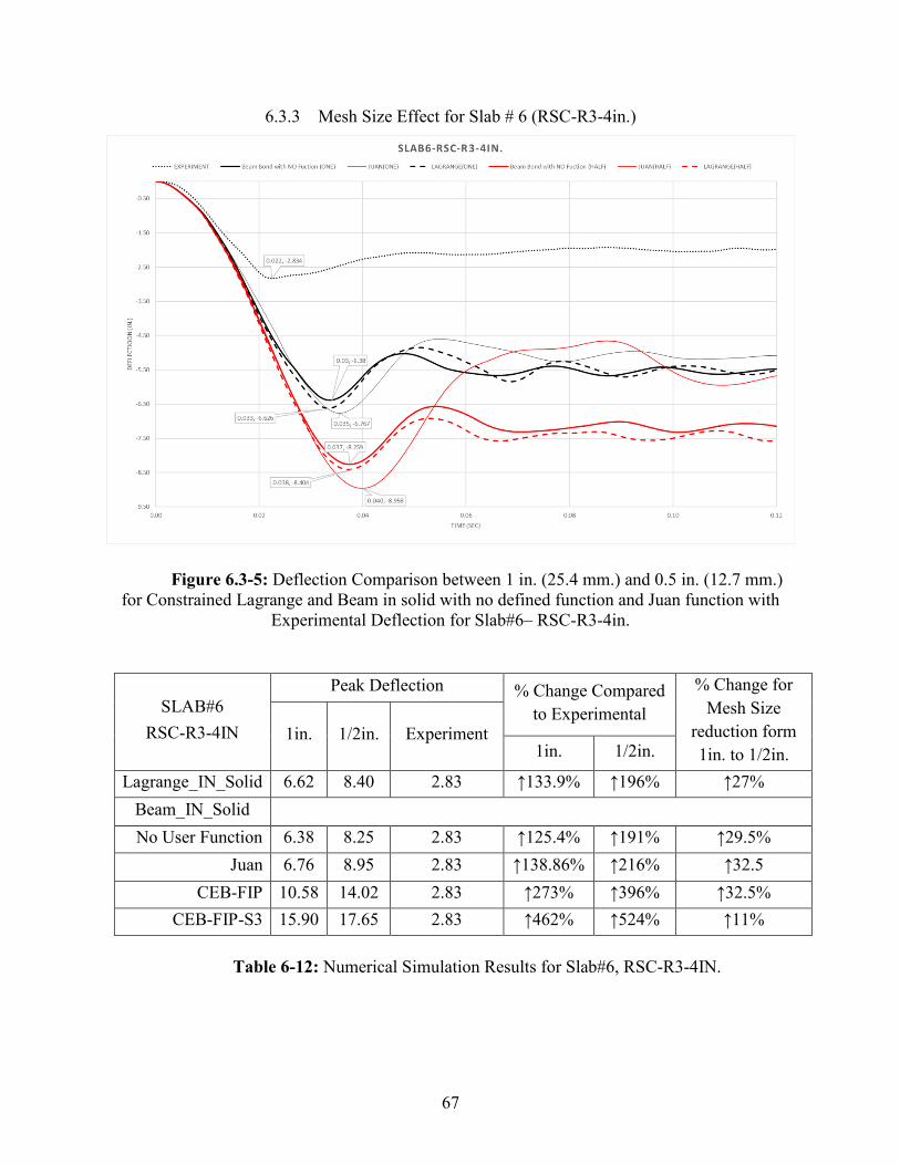
67
6.3.3 Mesh Size Effect for Slab # 6 (RSC-R3-4in.)
Figure 6.3-5: Deflection Comparison between 1 in. (25.4 mm.) and 0.5 in. (12.7 mm.)
for Constrained Lagrange and Beam in solid with no defined function and Juan function with
Experimental Deflection for Slab#6– RSC-R3-4in.
SLAB#6
RSC-R3-4IN
Peak Deflection % Change Compared
to Experimental
% Change for
Mesh Size
reduction form
1in. to 1/2in.
1in. 1/2in. Experiment 1in. 1/2in.
Lagrange_IN_Solid 6.62 8.40 2.83 ↑133.9% ↑196% ↑27%
Beam_IN_Solid
No User Function 6.38 8.25 2.83 ↑125.4% ↑191% ↑29.5%
Juan 6.76 8.95 2.83 ↑138.86% ↑216% ↑32.5
CEB-FIP 10.58 14.02 2.83 ↑273% ↑396% ↑32.5%
CEB-FIP-S3 15.90 17.65 2.83 ↑462% ↑524% ↑11%
Table 6-12: Numerical Simulation Results for Slab#6, RSC-R3-4IN.
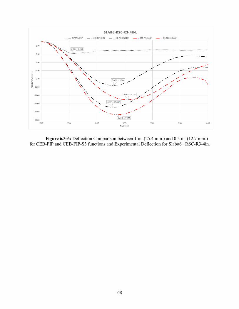
68
Figure 6.3-6: Deflection Comparison between 1 in. (25.4 mm.) and 0.5 in. (12.7 mm.)
for CEB-FIP and CEB-FIP-S3 functions and Experimental Deflection for Slab#6– RSC-R3-4in.
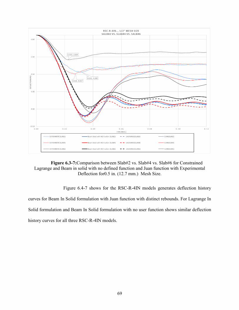
69
Figure 6.3-7:Comparison between Slab#2 vs. Slab#4 vs. Slab#6 for Constrained
Lagrange and Beam in solid with no defined function and Juan function with Experimental
Deflection for0.5 in. (12.7 mm.) Mesh Size.
Figure 6.4-7 shows for the RSC-R-4IN models generates deflection history
curves for Beam In Solid formulation with Juan function with distinct rebounds. For Lagrange In
Solid formulation and Beam In Solid formulation with no user function shows similar deflection
history curves for all three RSC-R-4IN models.
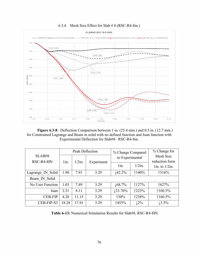
70
6.3.4 Mesh Size Effect for Slab # 8 (RSC-R4-8in.)
Figure 6.3-8 : Deflection Comparison between 1 in. (25.4 mm.) and 0.5 in. (12.7 mm.)
for Constrained Lagrange and Beam in solid with no defined function and Juan function with
Experimental Deflection for Slab#8– RSC-R4-8in.
SLAB#8
RSC-R4-8IN
Peak Deflection % Change Compared
to Experimental
% Change for
Mesh Size
reduction form
1in. to 1/2in.
1in. 1/2in. Experiment 1in. 1/2in.
Lagrange_IN_Solid 1.90 7.91 3.29 ↓42.2% ↑140% ↑316%
Beam_IN_Solid
No User Function 1.03 7.49 3.29 ↓68.7% ↑127% ↑627%
Juan 2.51 8.11 3.29 ↓23.70% ↑223% ↑160.5%
CEB-FIP 4.28 11.15 3.29 ↑30% ↑238% ↑160.5%
CEB-FIP-S3 18.28 17.91 3.29 ↑455% ↓2% ↓3.5%
Table 6-13: Numerical Simulation Results for Slab#8, RSC-R4-8IN.
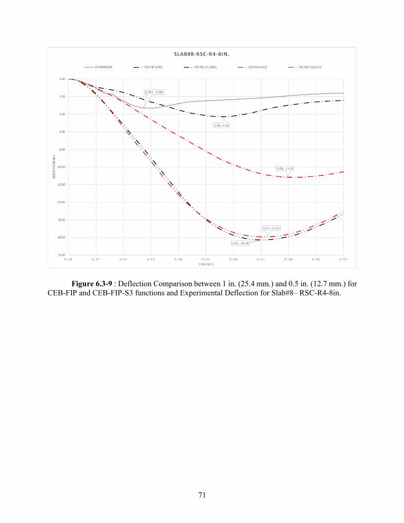
71
Figure 6.3-9 : Deflection Comparison between 1 in. (25.4 mm.) and 0.5 in. (12.7 mm.) for
CEB-FIP and CEB-FIP-S3 functions and Experimental Deflection for Slab#8– RSC-R4-8in.
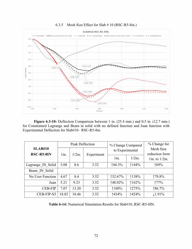
72
6.3.5 Mesh Size Effect for Slab # 10 (RSC-R5-8in.)
Figure 6.3-10: Deflection Comparison between 1 in. (25.4 mm.) and 0.5 in. (12.7 mm.)
for Constrained Lagrange and Beam in solid with no defined function and Juan function with
Experimental Deflection for Slab#10– RSC-R5-8in.
SLAB#10
RSC-R5-8IN
Peak Deflection % Change Compared
to Experimental
% Change for
Mesh Size
reduction form
1in. to 1/2in.
1in. 1/2in. Experiment 1in. 1/2in.
Lagrange_IN_Solid 5.08 8.6 3.52 ↑44.3% ↑144% ↑69%
Beam_IN_Solid
No User Function 4.67 8.4 3.52 ↑32.67% ↑138% ↑79.8%
Juan 5.21 9.23 3.52 ↑48.02% ↑162% ↑77%
CEB-FIP 7.07 13.20 3.52 ↑100% ↑275% ↑86.7%
CEB-FIP-S3 18.82 18.46 3.52 ↑434% ↑424% ↓1.91%
Table 6-14: Numerical Simulation Results for Slab#10, RSC-R5-8IN.
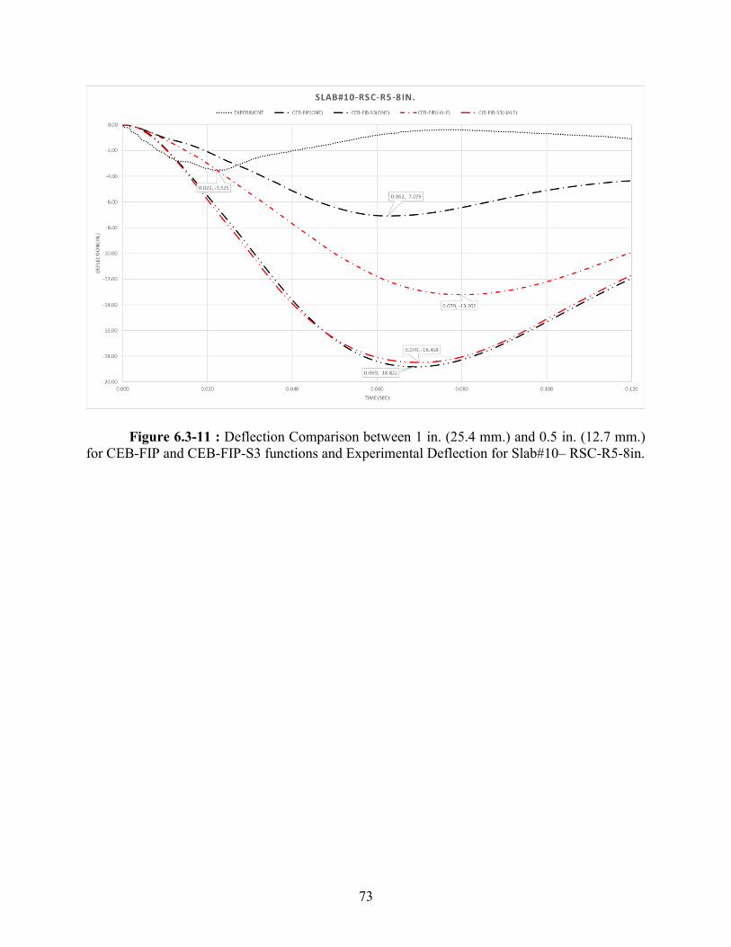
73
Figure 6.3-11 : Deflection Comparison between 1 in. (25.4 mm.) and 0.5 in. (12.7 mm.)
for CEB-FIP and CEB-FIP-S3 functions and Experimental Deflection for Slab#10– RSC-R5-8in.
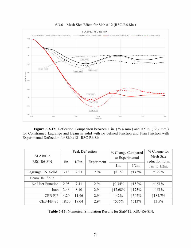
74
6.3.6 Mesh Size Effect for Slab # 12 (RSC-R6-8in.)
Figure 6.3-12: Deflection Comparison between 1 in. (25.4 mm.) and 0.5 in. (12.7 mm.)
for Constrained Lagrange and Beam in solid with no defined function and Juan function with
Experimental Deflection for Slab#12– RSC-R6-8in.
SLAB#12
RSC-R6-8IN
Peak Deflection % Change Compared
to Experimental
% Change for
Mesh Size
reduction form
1in. to 1/2in.
1in. 1/2in. Experiment 1in. 1/2in.
Lagrange_IN_Solid 3.18 7.23 2.94 ↑8.1% ↑145% ↑127%
Beam_IN_Solid
No User Function 2.95 7.41 2.94 ↑0.34% ↑152% ↑151%
Juan 3.46 8.10 2.94 ↑17.68% ↑175% ↑151%
CEB-FIP 4.20 11.96 2.94 ↑42% ↑307% ↑184.7%
CEB-FIP-S3 18.70 18.04 2.94 ↑536% ↑513% ↓3.5%
Table 6-15: Numerical Simulation Results for Slab#12, RSC-R6-8IN.
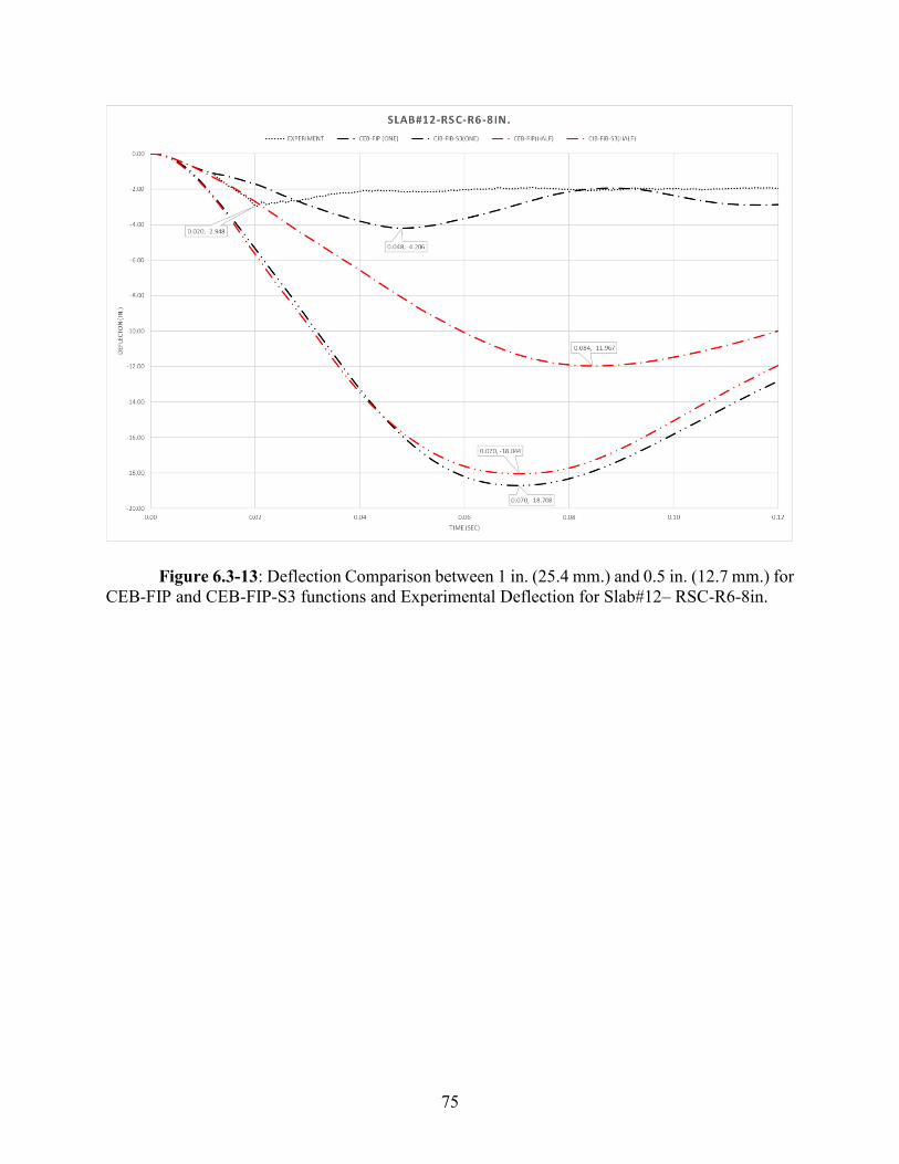
75
Figure 6.3-13: Deflection Comparison between 1 in. (25.4 mm.) and 0.5 in. (12.7 mm.) for
CEB-FIP and CEB-FIP-S3 functions and Experimental Deflection for Slab#12– RSC-R6-8in.
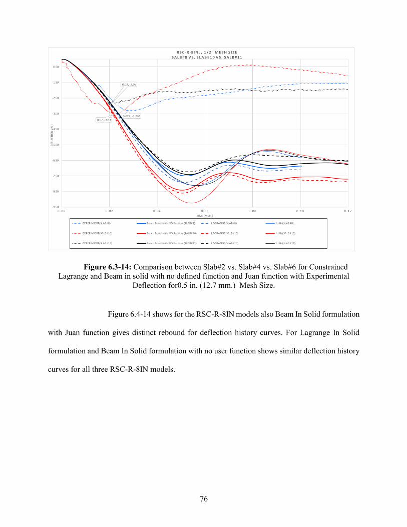
76
Figure 6.3-14: Comparison between Slab#2 vs. Slab#4 vs. Slab#6 for Constrained
Lagrange and Beam in solid with no defined function and Juan function with Experimental
Deflection for0.5 in. (12.7 mm.) Mesh Size.
Figure 6.4-14 shows for the RSC-R-8IN models also Beam In Solid formulation
with Juan function gives distinct rebound for deflection history curves. For Lagrange In Solid
formulation and Beam In Solid formulation with no user function shows similar deflection history
curves for all three RSC-R-8IN models.
77
CHAPTER 7. DISCUSSION OF RESULTS
Comparison of all the twelve slabs is carried out between numerical simulation
results and experimental data. Normal-strength concrete with normal-strength steel (RSC-R) and
high-strength concrete with high-strength steel (HSC-V) are the two material combinations used
for this comparison. These are discussed in detail in this chapter with the comparison criterion of
the deflection response of both the experimental and numerical analysis. High-Strength Concrete
– Comparison of Model with 1 in. (25.4 mm.) Mesh to ½ in. (12.7 mm.) Mesh Model.
The custom defined function for beam bond formulation also has similar change
in peak deflection when compared to experimental peak deflection. Whereas residual defection of
Juan function and CEB-FIP-S3 shows results of rhythm of the defection history curve which dies
once peak deflection is reached for most cases.
For ½ in. (12.7 mm.) mesh size is accurately able to predict peak deflection
history value for high strength material than1 in. (25.4 mm.). But the number of simulations runs
terminated are also more in comparison with 1 in. (25.4 mm.), mesh size. Juan function for beam-
bond formulation produced only two out of six results, whereas both CEB-FIP gave all six slabs
results. Both CEB-FIP functions tend to give more variation for 4in slabs in comparison to the 8in
slabs. Perfect bond formulation and beam-bond formulation generated by this program tended to
give more accurate results than all the three user defined functions for beam-bond formulation.
7.1 High-Strength Concrete – Comparison of Model with 1 in. (25.4 mm.) Mesh to ½ in. (12.7
mm.) Mesh Model.
Table 7-1: Analytical and Experimental Peak Slab Deflection Summary for High
Strength Slabs for 1 in. mesh size.
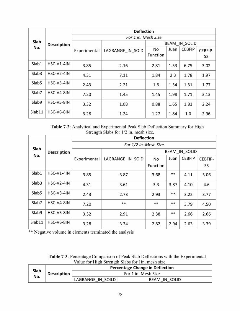
78
Slab No.
Description
Deflection
For 1 in. Mesh Size
Experimental LAGRANGE_IN_SOID
BEAM_IN_SOLID
No Function
Juan CEBFIP CEBFIP-S3
Slab1 HSC-V1-4IN 3.85 2.16 2.81 1.53 6.75 3.02
Slab3 HSC-V2-4IN 4.31 7.11 1.84 2.3 1.78 1.97
Slab5 HSC-V3-4IN 2.43 2.21 1.6 1.34 1.31 1.77
Slab7 HSC-V4-8IN 7.20 1.45 1.45 1.98 1.71 3.13
Slab9 HSC-V5-8IN 3.32 1.08 0.88 1.65 1.81 2.24
Slab11 HSC-V6-8IN 3.28 1.24 1.27 1.84 1.0 2.96
Table 7-2: Analytical and Experimental Peak Slab Deflection Summary for High
Strength Slabs for 1/2 in. mesh size.
Slab
No. Description
Deflection
For 1/2 in. Mesh Size
Experimental LAGRANGE_IN_SOID
BEAM_IN_SOLID
No
Function
Juan CEBFIP CEBFIP-
S3
Slab1 HSC-V1-4IN 3.85 3.87 3.68 ** 4.11 5.06
Slab3 HSC-V2-4IN 4.31 3.61 3.3 3.87 4.10 4.6
Slab5 HSC-V3-4IN 2.43 2.73 2.93 ** 3.22 3.77
Slab7 HSC-V4-8IN 7.20 ** ** ** 3.79 4.50
Slab9 HSC-V5-8IN 3.32 2.91 2.38 ** 2.66 2.66
Slab11 HSC-V6-8IN 3.28 3.34 2.82 2.94 2.63 3.39
** Negative volume in elements terminated the analysis
Table 7-3: Percentage Comparison of Peak Slab Deflections with the Experimental
Value for High Strength Slabs for 1in. mesh size.
Slab No.
Description
Percentage Change in Deflection
For 1 in. Mesh Size
LAGRANGE_IN_SOILD BEAM_IN_SOLID
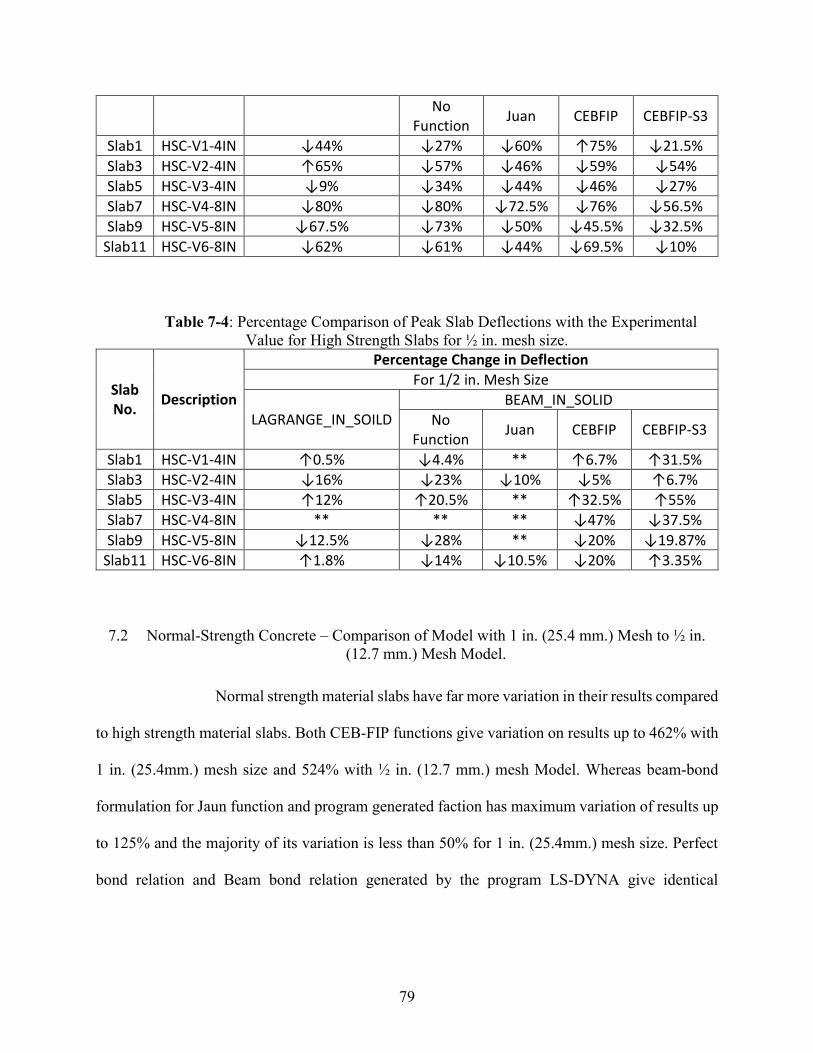
79
No Function
Juan CEBFIP CEBFIP-S3
Slab1 HSC-V1-4IN ↓44% ↓27% ↓60% ↑75% ↓21.5%
Slab3 HSC-V2-4IN ↑65% ↓57% ↓46% ↓59% ↓54%
Slab5 HSC-V3-4IN ↓9% ↓34% ↓44% ↓46% ↓27%
Slab7 HSC-V4-8IN ↓80% ↓80% ↓72.5% ↓76% ↓56.5%
Slab9 HSC-V5-8IN ↓67.5% ↓73% ↓50% ↓45.5% ↓32.5%
Slab11 HSC-V6-8IN ↓62% ↓61% ↓44% ↓69.5% ↓10%
Table 7-4: Percentage Comparison of Peak Slab Deflections with the Experimental
Value for High Strength Slabs for ½ in. mesh size.
Slab No.
Description
Percentage Change in Deflection
For 1/2 in. Mesh Size
LAGRANGE_IN_SOILD BEAM_IN_SOLID
No Function
Juan CEBFIP CEBFIP-S3
Slab1 HSC-V1-4IN ↑0.5% ↓4.4% ** ↑6.7% ↑31.5%
Slab3 HSC-V2-4IN ↓16% ↓23% ↓10% ↓5% ↑6.7%
Slab5 HSC-V3-4IN ↑12% ↑20.5% ** ↑32.5% ↑55%
Slab7 HSC-V4-8IN ** ** ** ↓47% ↓37.5%
Slab9 HSC-V5-8IN ↓12.5% ↓28% ** ↓20% ↓19.87%
Slab11 HSC-V6-8IN ↑1.8% ↓14% ↓10.5% ↓20% ↑3.35%
7.2 Normal-Strength Concrete – Comparison of Model with 1 in. (25.4 mm.) Mesh to ½ in.
(12.7 mm.) Mesh Model.
Normal strength material slabs have far more variation in their results compared
to high strength material slabs. Both CEB-FIP functions give variation on results up to 462% with
1 in. (25.4mm.) mesh size and 524% with ½ in. (12.7 mm.) mesh Model. Whereas beam-bond
formulation for Jaun function and program generated faction has maximum variation of results up
to 125% and the majority of its variation is less than 50% for 1 in. (25.4mm.) mesh size. Perfect
bond relation and Beam bond relation generated by the program LS-DYNA give identical
80
deflection history curves in their results, in most cases, for both mesh sizes, and have less variation
between them.
The nature of residual deflection history curve for Juan function is similar for
most of the twelve slabs, which is not affected by reinforcement ratio. For 1 in. (25.4mm.) mesh
size all the residual deflection curve are similar and for all ½ in. (12.7 mm.) mesh size all the
residual deflection curve are also similar. In the case of both CEB-FIP functions there is no chance
to comment on residual deflection.
For the reduction of the mesh size form 1 in. (25.4mm.) to ½ in. (12.7 mm.)
peak deflection tends to increase. CIB-FIP-S3 function for beam-bond formulation give less
reduction when mesh size is decreased than other bond functions.
The overall mesh analysis results for all six slabs of regular material strength
are tabulated in the Table 7.2-1 to Table 7.2-4. The Table 7.2-1 and Table 7.2-2 gives peak
deflection for 1 in. (25.4 mm) and ½ in. (12.7 mm) mesh size respectively. Table 7.2-3 and Table
7.2-4 gives percentage change in peck deflection for same with respect to the experimental peak
deflections.
Table 7-5: Analytical and Experimental Peak Slab Deflection Summary for Regular
Strength Slabs for 1 in. mesh size.
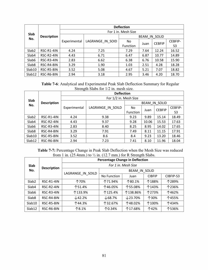
81
Slab No.
Description
Deflection
For 1 in. Mesh Size
Experimental LAGRANGE_IN_SOID BEAM_IN_SOLID
No Function
Juan CEBFIP CEBFIP-
S3
Slab2 RSC-R1-4IN 4.24 7.25 7.29 7.64 12.24 16.52
Slab4 RSC-R2-4IN 4.43 6.71 6.47 6.87 10.77 14.89
Slab6 RSC-R3-4IN 2.83 6.62 6.38 6.76 10.58 15.90
Slab8 RSC-R4-8IN 3.29 1.90 1.03 2.51 4.28 18.28
Slab10 RSC-R5-8IN 3.52 5.08 4.67 5.21 7.07 18.82
Slab12 RSC-R6-8IN 2.94 3.18 2.95 3.46 4.20 18.70
Table 7-6: Analytical and Experimental Peak Slab Deflection Summary for Regular
Strength Slabs for 1/2 in. mesh size.
Slab No.
Description
Deflection
For 1/2 in. Mesh Size
Experimental LAGRANGE_IN_SOILD BEAM_IN_SOLID
No Function
Juan CEBFIP CEBFIP-
S3
Slab2 RSC-R1-4IN 4.24 9.38 9.23 9.89 15.14 18.49
Slab4 RSC-R2-4IN 4.43 9.37 9.28 10.06 15.53 17.63
Slab6 RSC-R3-4IN 2.83 8.40 8.25 8.95 14.02 17.65
Slab8 RSC-R4-8IN 3.29 7.91 7.49 8.11 11.15 17.91
Slab10 RSC-R5-8IN 3.52 8.6 8.4 9.23 13.20 18.46
Slab12 RSC-R6-8IN 2.94 7.23 7.41 8.10 11.96 18.04
Table 7-7: Percentage Change in Peak Slab Deflection when the Mesh Size was reduced
from 1 in. (25.4mm.) to ½ in. (12.7 mm.) for R Strength Slabs.
Slab No.
Description
Percentage Change in Deflection
For 1 in. Mesh Size
LAGRANGE_IN_SOILD BEAM_IN_SOLID
No Function Juan CIBFIP CIBFIP-S3
Slab2 RSC-R1-4IN ↑70% ↑71.94% ↑80.1% ↑188% ↑289%
Slab4 RSC-R2-4IN ↑51.4% ↑46.05% ↑55.08% ↑143% ↑236%
Slab6 RSC-R3-4IN ↑133.9% ↑125.4% ↑138.86% ↑273% ↑462%
Slab8 RSC-R4-8IN ↓42.2% ↓68.7% ↓23.70% ↑30% ↑455%
Slab10 RSC-R5-8IN ↑44.3% ↑32.67% ↑48.02% ↑100% ↑434%
Slab12 RSC-R6-8IN ↑8.1% ↑0.34% ↑17.68% ↑42% ↑536%
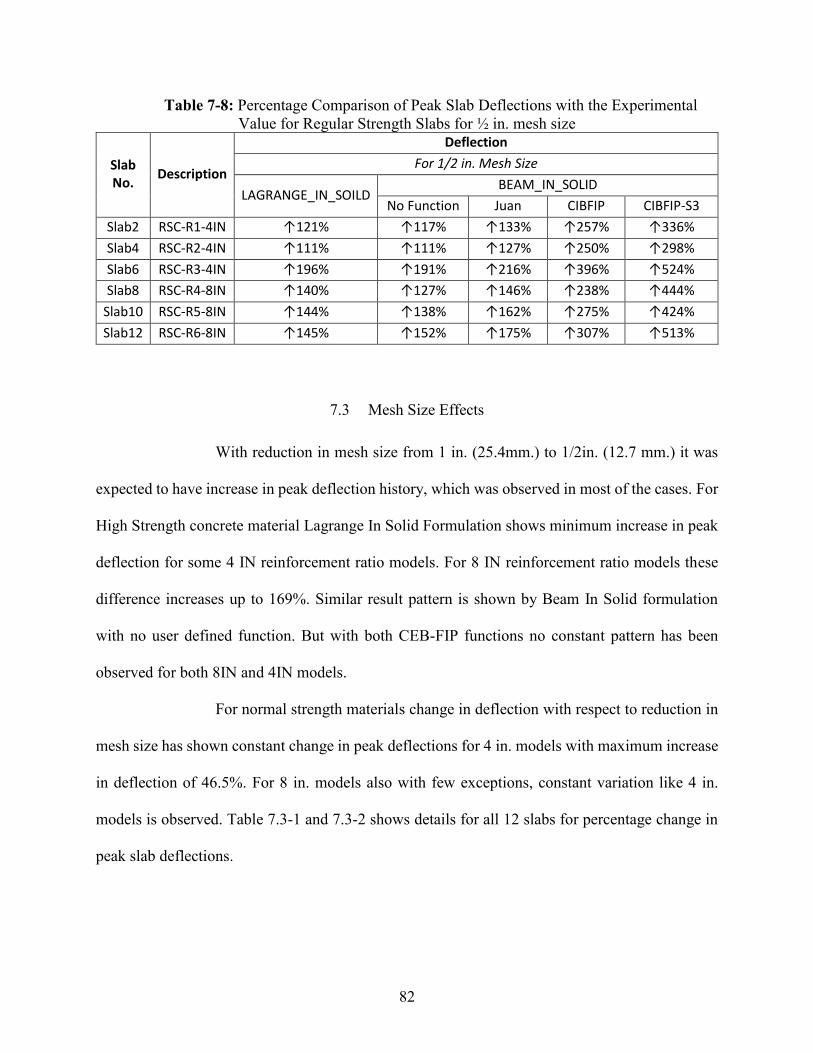
82
Table 7-8: Percentage Comparison of Peak Slab Deflections with the Experimental
Value for Regular Strength Slabs for ½ in. mesh size
Slab No.
Description
Deflection
For 1/2 in. Mesh Size
LAGRANGE_IN_SOILD BEAM_IN_SOLID
No Function Juan CIBFIP CIBFIP-S3
Slab2 RSC-R1-4IN ↑121% ↑117% ↑133% ↑257% ↑336%
Slab4 RSC-R2-4IN ↑111% ↑111% ↑127% ↑250% ↑298%
Slab6 RSC-R3-4IN ↑196% ↑191% ↑216% ↑396% ↑524%
Slab8 RSC-R4-8IN ↑140% ↑127% ↑146% ↑238% ↑444%
Slab10 RSC-R5-8IN ↑144% ↑138% ↑162% ↑275% ↑424%
Slab12 RSC-R6-8IN ↑145% ↑152% ↑175% ↑307% ↑513%
7.3 Mesh Size Effects
With reduction in mesh size from 1 in. (25.4mm.) to 1/2in. (12.7 mm.) it was
expected to have increase in peak deflection history, which was observed in most of the cases. For
High Strength concrete material Lagrange In Solid Formulation shows minimum increase in peak
deflection for some 4 IN reinforcement ratio models. For 8 IN reinforcement ratio models these
difference increases up to 169%. Similar result pattern is shown by Beam In Solid formulation
with no user defined function. But with both CEB-FIP functions no constant pattern has been
observed for both 8IN and 4IN models.
For normal strength materials change in deflection with respect to reduction in
mesh size has shown constant change in peak deflections for 4 in. models with maximum increase
in deflection of 46.5%. For 8 in. models also with few exceptions, constant variation like 4 in.
models is observed. Table 7.3-1 and 7.3-2 shows details for all 12 slabs for percentage change in
peak slab deflections.
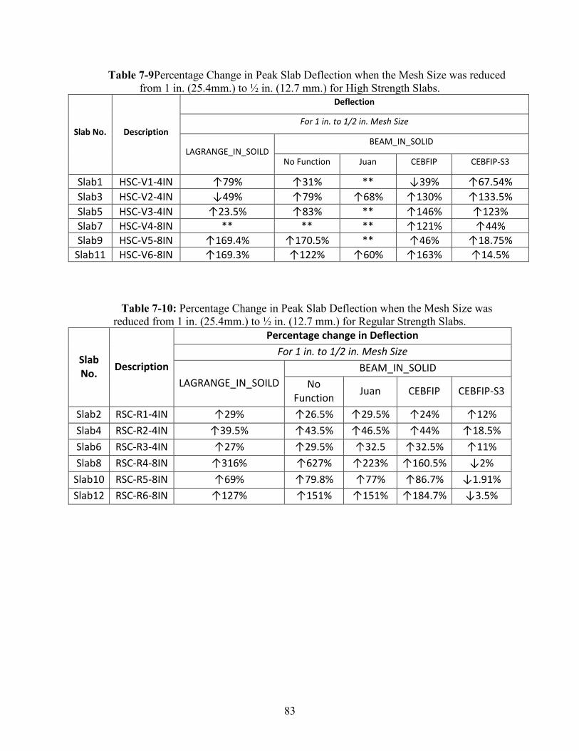
83
Table 7-9Percentage Change in Peak Slab Deflection when the Mesh Size was reduced
from 1 in. (25.4mm.) to ½ in. (12.7 mm.) for High Strength Slabs.
Slab No. Description
Deflection
For 1 in. to 1/2 in. Mesh Size
LAGRANGE_IN_SOILD BEAM_IN_SOLID
No Function Juan CEBFIP CEBFIP-S3
Slab1 HSC-V1-4IN ↑79% ↑31% ** ↓39% ↑67.54%
Slab3 HSC-V2-4IN ↓49% ↑79% ↑68% ↑130% ↑133.5%
Slab5 HSC-V3-4IN ↑23.5% ↑83% ** ↑146% ↑123%
Slab7 HSC-V4-8IN ** ** ** ↑121% ↑44%
Slab9 HSC-V5-8IN ↑169.4% ↑170.5% ** ↑46% ↑18.75%
Slab11 HSC-V6-8IN ↑169.3% ↑122% ↑60% ↑163% ↑14.5%
Table 7-10: Percentage Change in Peak Slab Deflection when the Mesh Size was
reduced from 1 in. (25.4mm.) to ½ in. (12.7 mm.) for Regular Strength Slabs.
Slab No.
Description
Percentage change in Deflection
For 1 in. to 1/2 in. Mesh Size
LAGRANGE_IN_SOILD
BEAM_IN_SOLID
No Function
Juan CEBFIP CEBFIP-S3
Slab2 RSC-R1-4IN ↑29% ↑26.5% ↑29.5% ↑24% ↑12%
Slab4 RSC-R2-4IN ↑39.5% ↑43.5% ↑46.5% ↑44% ↑18.5%
Slab6 RSC-R3-4IN ↑27% ↑29.5% ↑32.5 ↑32.5% ↑11%
Slab8 RSC-R4-8IN ↑316% ↑627% ↑223% ↑160.5% ↓2%
Slab10 RSC-R5-8IN ↑69% ↑79.8% ↑77% ↑86.7% ↓1.91%
Slab12 RSC-R6-8IN ↑127% ↑151% ↑151% ↑184.7% ↓3.5%
84
CHAPTER 8. CONCLUSION AND FUTURE WORK
This chapter discusses conclusions and observations of the results of
comparison of numerical simulation experimental records of all twelve single-mat reinforced
concrete slabs, which were subjected to blast loading. Further results obtained were compared to
experimental data in order to validate bond interactions between concrete and steel. Further, in this
chapter, the scope for future work is also outlined based on the results and conclusions of this
study.
1. Prefect bond formulation using Lagrange In solid Formulation gives most accurate
results for peak deflection when compared to experimental records. Beam In Solid
formulation fails to give accurate results for blast loading,
2. If Beam In solid formulation is to be used than CEB-FIP-S3 function is most
appropriate function for high strength material and bond-slip function defined by Juan
for regular strength concrete is most appropriate.
3. Modification of CEB-FIP function by inclusion of new parameter can control free
vibration of slab after peak deflection is reached.
4. Winfrith concrete Model is unable to produces results which can be compared to
experimental records, hence its use for bond-slip analysis is not recommended.
5. ¼ inch (6.23 mm.) mesh size is unable to generate deflection history curves with normal
termination for analysis.

85
8.1 Future Scope of Work
The suggestions for future work are obtained from studies conducted in this
thesis and are given below.
1. The scope of improvement of beam-bond formulation functions which can address
material strength of concrete used to predict response more accurately in comparison
of experiment records for normal strength-concrete.
2. Based on experimental data available for single–mat slabs pressure- impulse diagrams
can be developed.
3. Use of hourglass control needs to be studied as it influences peak deflection history of
numerical simulation and developing relation between its parameters and the strength
of concrete used.
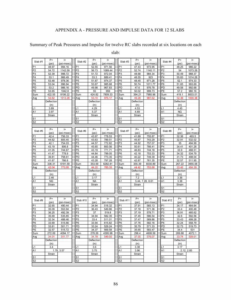
86
APPENDIX A - PRESSURE AND IMPULSE DATA FOR 12 SLABS
Summary of Peak Pressures and Impulse for twelve RC slabs recorded at six locations on each
slab:
P+ I+ P+ I+ P+ I+ P+ I+
(psi) (psi-msec) (psi) (psi-msec) (psi) (psi-msec) (psi) (psi-msec)
P1 48.97 994.16 P1 52.55 971.56 P1 47.43 973.95 P1 48.25 986.22
P2 54.72 1142.59 P2 56.73 1089.44 P2 52.74 1140.11 P2 54 1073.28
P3 52.39 998.72 P3 51.72 972.04 P3 48.68 984.34 P3 50.49 988.37
P4 53.1 966.49 P4 53.3 889.41 P4 48.55 923 P4 55.83 1014.28
P5 53.48 978.36 P5 51.87 974.37 P5 48.45 971.28 P5 52.1 974.33
P6 53.04 996.94 P6 53.67 985.68 P6 50.74 1011.77 P6 51.65 993.69
PD 53.2 986.16 PD 49.98 967.83 PD 47.6 976.78 PD 49.58 992.68
PE 53.65 1042.8 PE 55 959 PE 50.02 999.73 PE 57.2 980.16
Sum 422.55 8106.22 Sum 424.82 7809.33 Sum 394.21 7980.96 Sum 419.1 8003.01
Avg 52.82 1013.28 Avg 53.10 976.17 Avg 49.28 997.62 Avg 52.39 1000.38
Deflection Deflection Deflection Deflection
(in) (in) (in) (in)
L1 3.89 L1 4.29 L1 4.53 L1 4.45
A1 3.97 A1 5.37 A1 4.69 A1 NG
Strain Strain Strain Strain
S1 S1 S1 S1
S2 S2 S2 S2
P+ I+ P+ I+ P+ I+ P+ I+
(psi) (psi-msec) (psi) (psi-msec) (psi) (psi-msec) (psi) (psi-msec)
P1 42.4 756.33 P1 43.97 778.53 P1 41.89 755.87 P1 32.38 493.5
P2 44.62 805.45 P2 43.63 789.51 P2 45.87 743.29 P2 32.91 532.02
P3 42.1 754.03 P3 44.57 772.82 P3 44.92 757.07 P3 35 494.99
P4 43.19 806.8 P4 45.65 800.56 P4 50.61 766.41 P4 34.41 401.28
P5 41.05 744.67 P5 43.19 771.71 P5 46.83 744.18 P5 33.9 488.51
P6 41.47 778.9 P6 44.84 799.05 P6 42.18 753.33 P6 34.32 534.79
PD 39.81 758.61 PD 44.46 773.35 PD 40.22 749.39 PD 31.73 498.04
PE 41.67 786.8 PE 43.28 797.28 PE 42.87 761.35 PE 32.57 511.95
Sum 336.31 6191.59 Sum 353.59 6282.81 Sum 355.39 6030.89 Sum 267.22 3955.08
Avg 42.04 773.95 Avg 44.20 785.35 Avg 44.42 753.86 Avg 33.40 494.39
Deflection Deflection Deflection Deflection
(in) (in) (in) (in)
L1 2.46 L1 3.17 L1 7.2 L1 3.36
A1 NG A1 NA A1 A1 3.38
Strain Strain Strain Strain
S1 S1 S1 S1
S2 S2 S2 S2
P+ I+ P+ I+ P+ I+ P+ I+
(psi) (psi-msec) (psi) (psi-msec) (psi) (psi-msec) (psi) (psi-msec)
P1 32.65 490.44 P1 34.94 518.32 P1 37.91 565.13 P1 34.17 484.64
P2 35.09 553.94 P2 36.43 549.86 P2 37.18 571.36 P2 33.4 400.48
P3 36.25 492.39 P3 37 519.8 P3 37.19 578.71 P3 36.91 485.62
P4 35.69 535.85 P4 34.94 582.35 P4 37.45 586.54 P4 32.6 592.56
P5 32.34 488.46 P5 33.4 511.01 P5 37.47 569.86 P5 33.43 499.28
P6 33.69 515.66 P6 33.94 615.82 P6 37.76 582.16 P6 32.24 558.79
PD 33.81 501.71 PD 33.24 529.24 PD 35.79 571.33 PD 32.73 519.73
PE 32.57 515.72 PE 34.37 569.58 PE 35.65 583.47 PE 34.4 531
Sum 272.09 4094.17 Sum 278.26 4395.98 Sum 296.4 4608.56 Sum 269.88 4072.1
Avg 34.01 511.77 Avg 34.78 549.50 Avg 37.05 576.07 Avg 33.74 509.01
Deflection Deflection Deflection Deflection
(in) (in) (in) (in)
L1 3.4 L1 3.6 L1 3.38 L1 3.17
A1 A1 3.75 A1 3.96 A1
Strain Strain Strain Strain
S1 S1 S1 S1
S2 S2 S2 S2
1.78, 3.57 2.12, 2.85
Slab #4
Slab #8
Slab #9 Slab #10 Slab #11 Slab #12
Slab #1 Slab #2 Slab #3
Slab #5 Slab #6 Slab #7
5.44, 7.28, 8.61
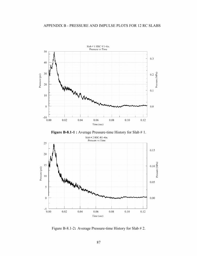
87
APPENDIX B - PRESSURE AND IMPULSE PLOTS FOR 12 RC SLABS
Figure B-8.1-1 : Average Pressure-time History for Slab # 1.
Figure B-8.1-2: Average Pressure-time History for Slab # 2.
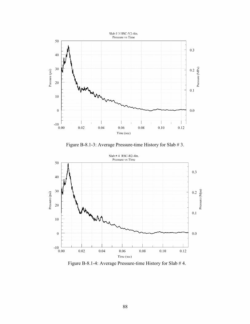
88
Figure B-8.1-3: Average Pressure-time History for Slab # 3.
Figure B-8.1-4: Average Pressure-time History for Slab # 4.
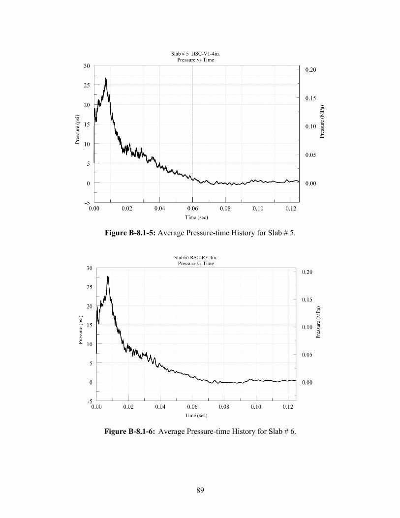
89
Figure B-8.1-5: Average Pressure-time History for Slab # 5.
Figure B-8.1-6: Average Pressure-time History for Slab # 6.
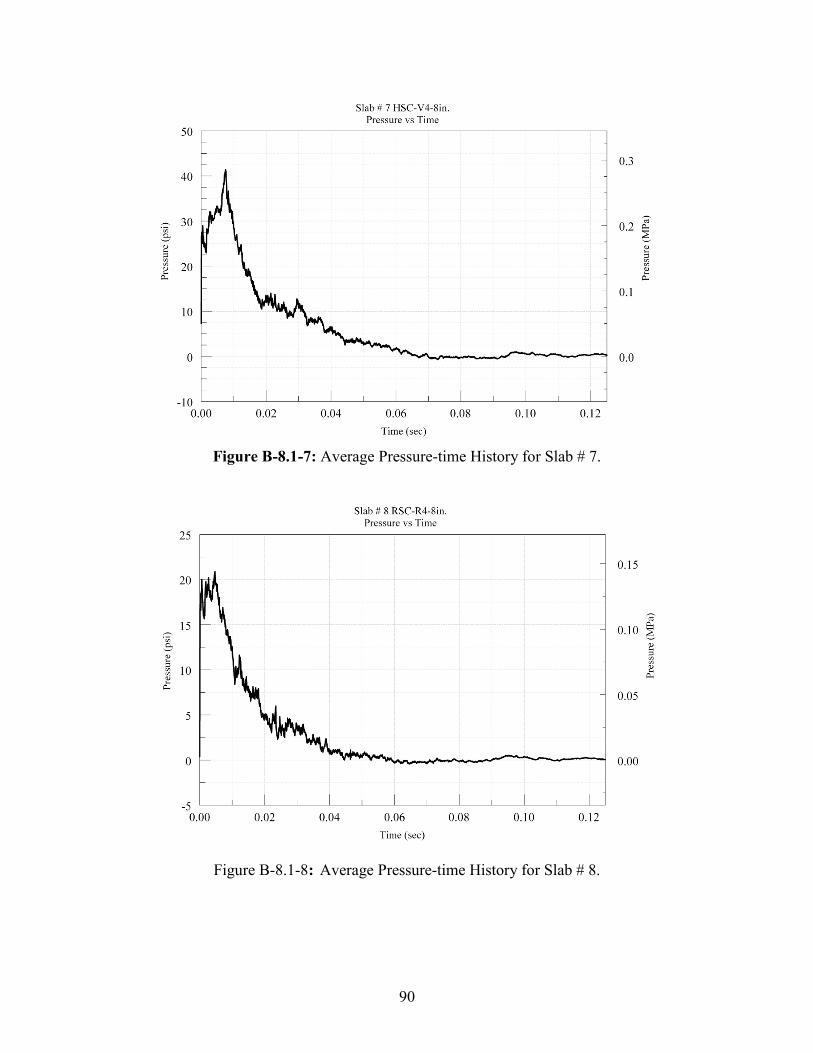
90
Figure B-8.1-7: Average Pressure-time History for Slab # 7.
Figure B-8.1-8: Average Pressure-time History for Slab # 8.
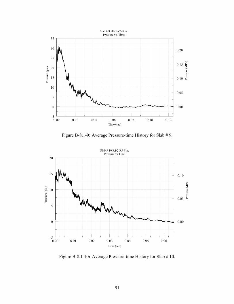
91
Figure B-8.1-9: Average Pressure-time History for Slab # 9.
Figure B-8.1-10: Average Pressure-time History for Slab # 10.
92
Figure B-8.1-11: Average Pressure-time History for Slab # 11.
Figure B-8.1-12: Average Pressure-time History for Slab # 12.
93
APPENDIX C - SUMMARY TABLES
Table C- 0-1: Input parameters for Concrete Damage Model Release 3
Variable Description Input value for
High strength
concrete
Input value for
Normal strength
concrete
RHO Mass Density 2.24E-04 lb-s/in3 2.24E-04 lb-s/in3
PR Poisson’s Ratio 0.18 0.18
FT Uniaxial Tensile Strength 928 psi 462psi
A0/-fc’ Uniaxial Compressive Strength 4700 3200
A1 Maximum shear surface parameter 0.55 0.60
A2 Maximum shear failure parameter 0.0000082 0.00000152
B1 Damage Scaling Parameter 1.6 1.6
OMEGA Fractional dilatancy 0.5 0.5
A1F Residual Failure Coefficient 0.4417 0.4417
Sλ Stretch factor 100 100
NOUT Output selector for effective plastic
strain
2 2
RSIZE Unit Conversion factor for length 1 1
UCF Unit Conversion factor for stress 1 1
LCRATE Load Curve for strain rate effects 0 0
LOCWID Maximum aggregate diameter 1 1
λ01-λ13 Damage Functions default default
B3 Damage scaling coefficient for tri-
axial tension
1.15 1.15
A0Y Initial yield surface cohesion 3460 1500
A1Y Initial yield surface coefficient 0.625 0.625
η01-η13 Scale factor default default
94
B2 Tensile Damage scaling coefficient 1.35 1.35
A2F Residual failure surface coefficient 0.00000763 0.0000177
A2Y Initial yield surface coefficient 0.0000166 0.0000384
Table C- 0-2: Input Parameters for Plastic Kinematic Model for Steel Rebar
Variable Description Input value for
High strength steel
Input value for
Normal strength
steel
RO Mass Density 7.30E-04 lb-s/in3 7.30E-04 lb-s/in3
E Young’s Modulus of Rebar 2.90E+07 psi 2.90E+07 psi
PR Poisson’s Ratio 3.00E-01 psi 3.00E-01 psi
SIGY Yield strength of Rebar 83000 psi 60000 psi
ETAN Tangent Modulus Default Default
BETA Hardening Parameter Default Default
SRC Strain Rate Parameter Default Default
SRP Strain Rate Parameter Default Default
FS Failure Strain for Eroding Elements Default Default
95
APPENDIX D – LS-DYNA INPUT
Figure D - 8.1-1 : Input and Output Control Parameters
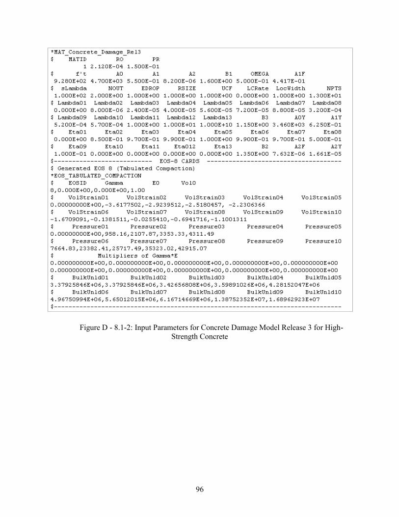
96
Figure D - 8.1-2: Input Parameters for Concrete Damage Model Release 3 for High-
Strength Concrete
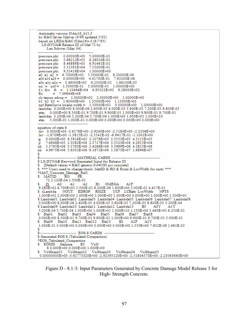
97
Figure D - 8.1-3: Input Parameters Generated by Concrete Damage Model Release 3 for
High- Strength Concrete.
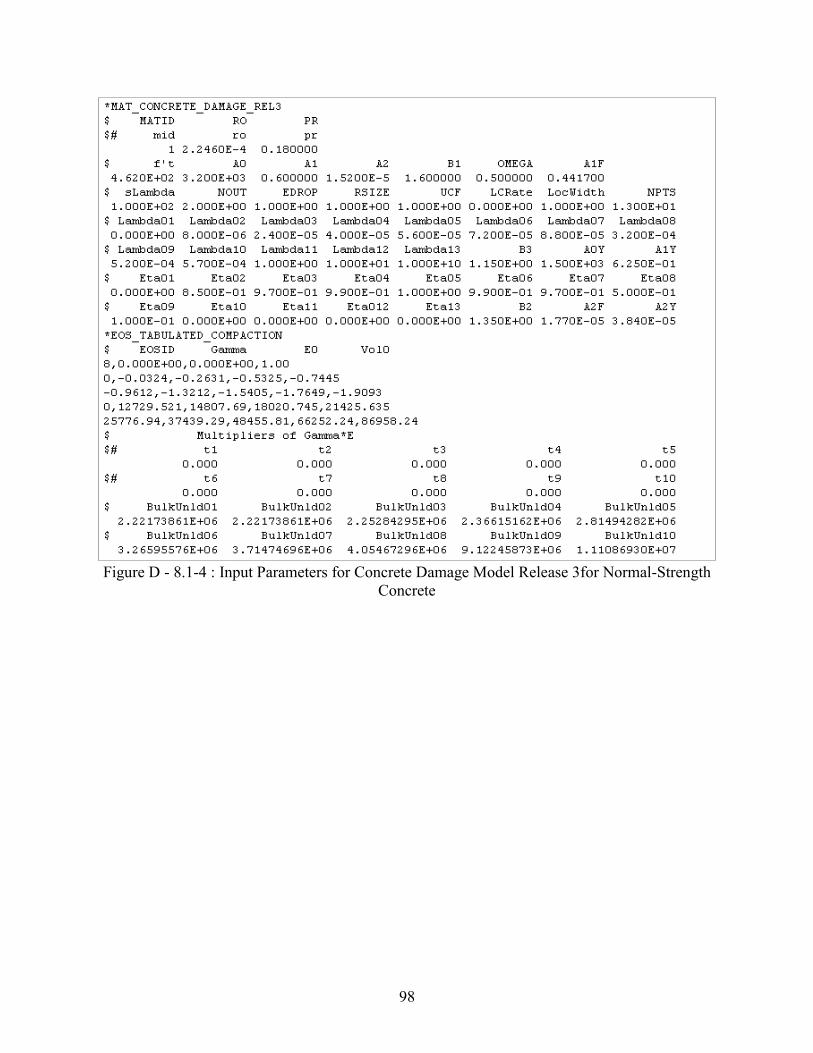
98
Figure D - 8.1-4 : Input Parameters for Concrete Damage Model Release 3for Normal-Strength
Concrete
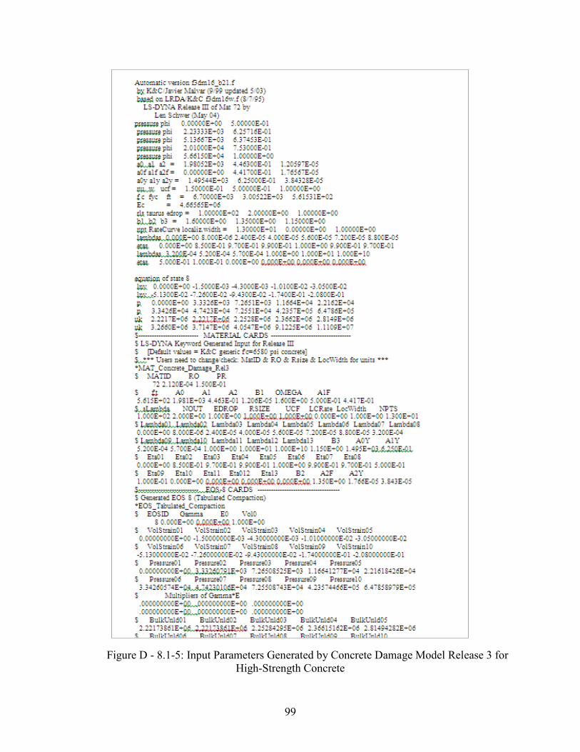
99
Figure D - 8.1-5: Input Parameters Generated by Concrete Damage Model Release 3 for
High-Strength Concrete
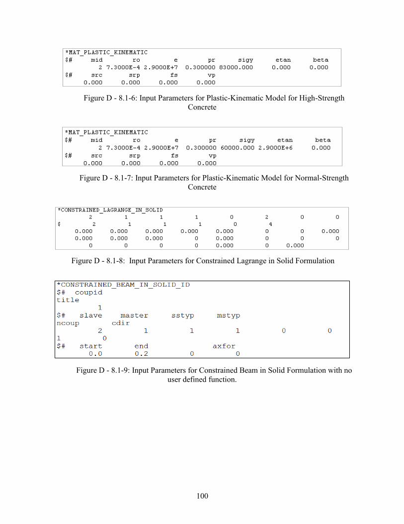
100
Figure D - 8.1-6: Input Parameters for Plastic-Kinematic Model for High-Strength
Concrete
Figure D - 8.1-7: Input Parameters for Plastic-Kinematic Model for Normal-Strength
Concrete
Figure D - 8.1-8: Input Parameters for Constrained Lagrange in Solid Formulation
Figure D - 8.1-9: Input Parameters for Constrained Beam in Solid Formulation with no
user defined function.
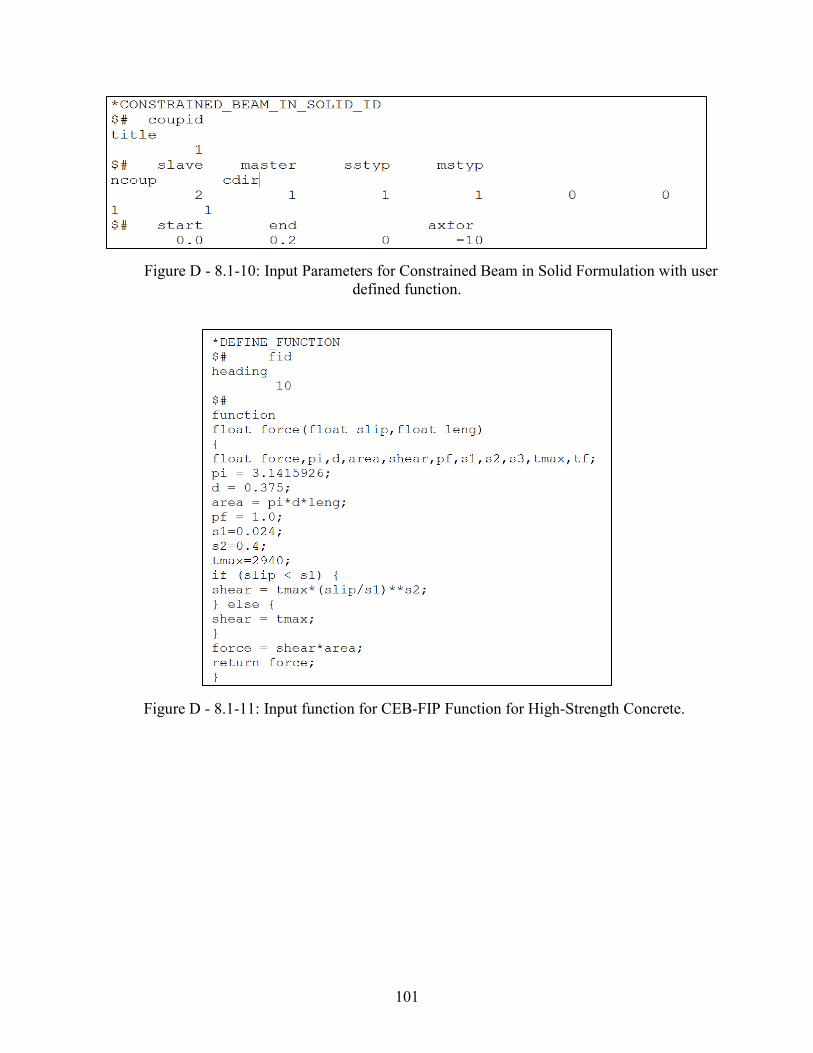
101
Figure D - 8.1-10: Input Parameters for Constrained Beam in Solid Formulation with user
defined function.
Figure D - 8.1-11: Input function for CEB-FIP Function for High-Strength Concrete.
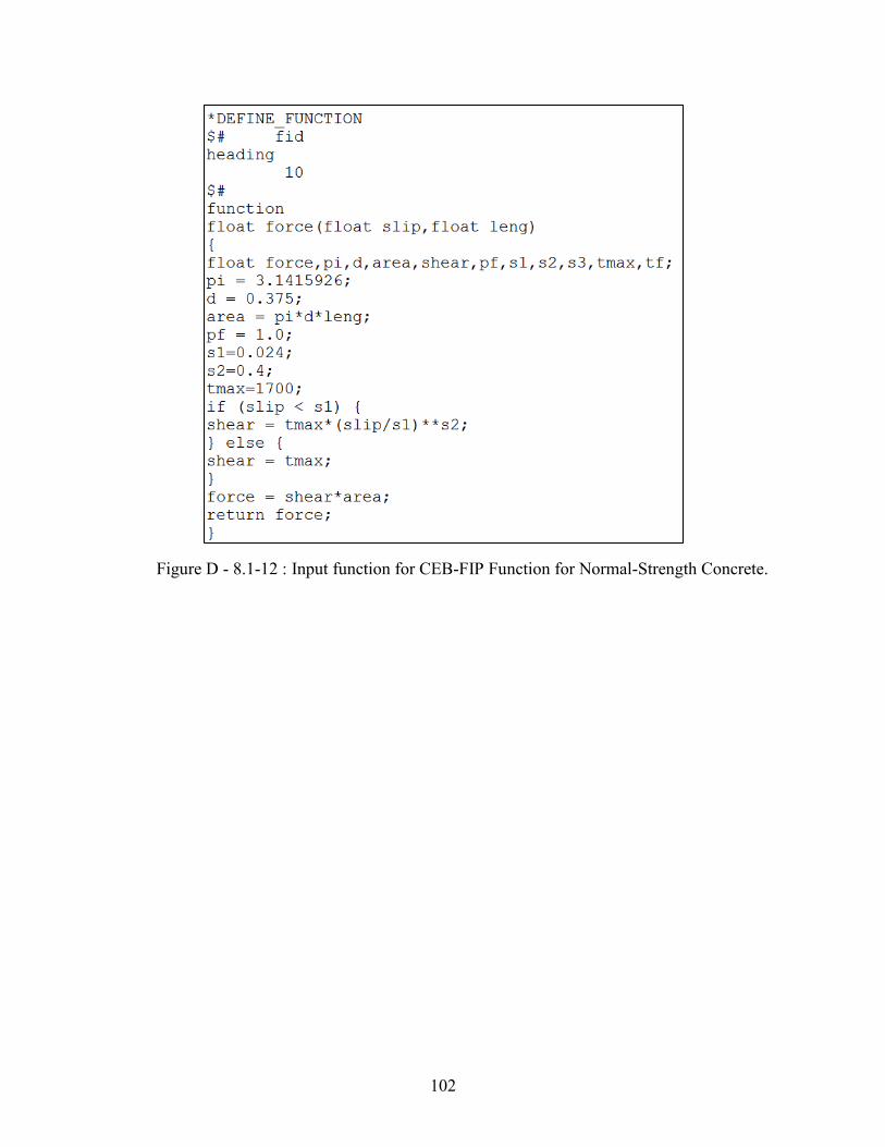
102
Figure D - 8.1-12 : Input function for CEB-FIP Function for Normal-Strength Concrete.
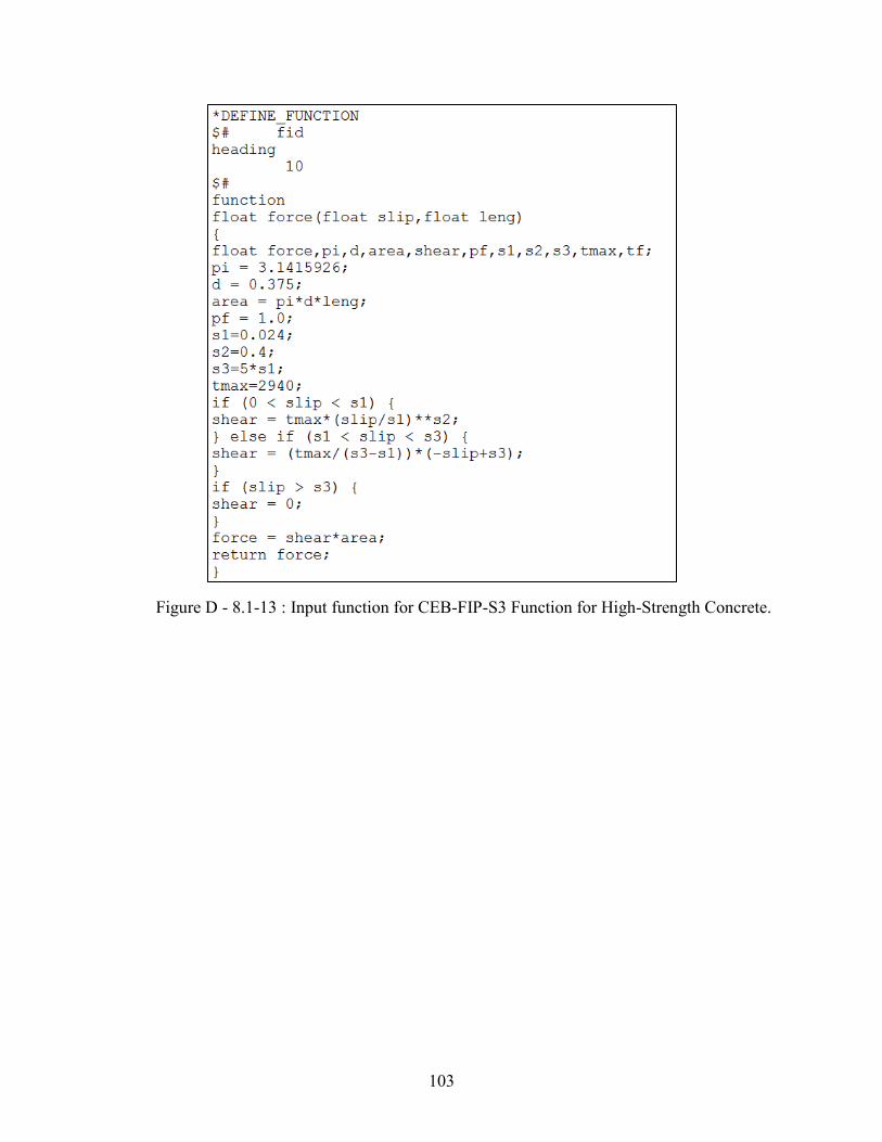
103
Figure D - 8.1-13 : Input function for CEB-FIP-S3 Function for High-Strength Concrete.
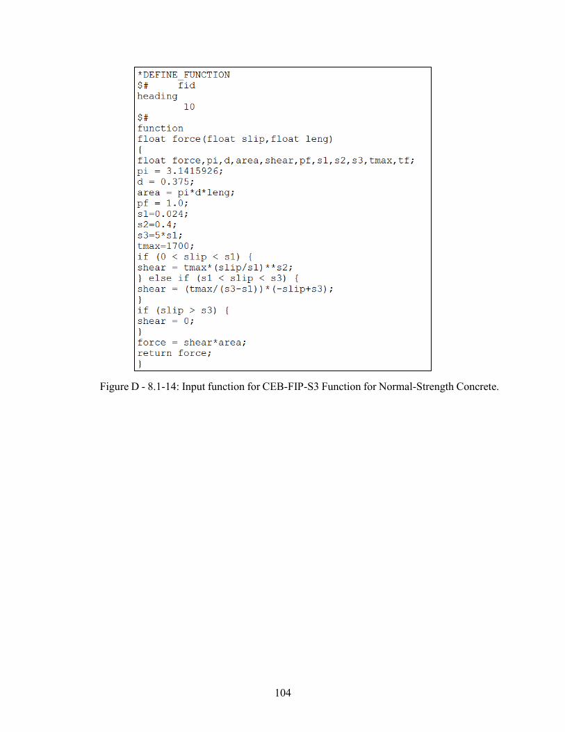
104
Figure D - 8.1-14: Input function for CEB-FIP-S3 Function for Normal-Strength Concrete.
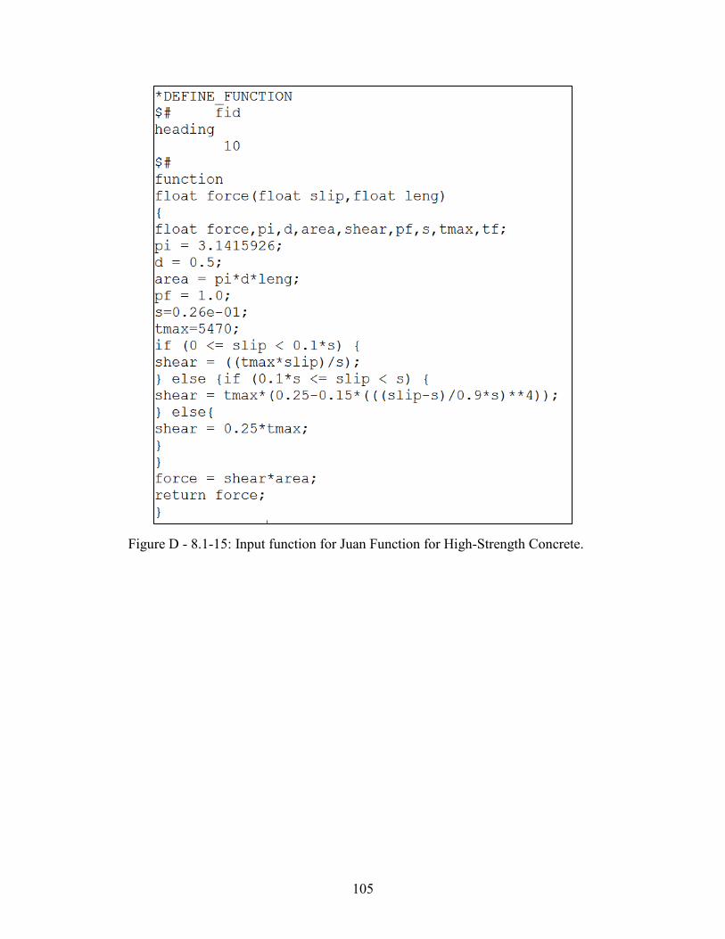
105
Figure D - 8.1-15: Input function for Juan Function for High-Strength Concrete.
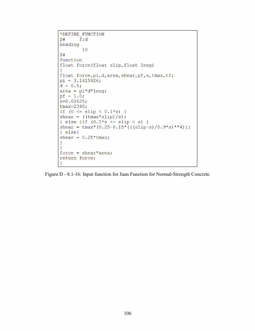
106
Figure D - 8.1-16: Input function for Juan Function for Normal-Strength Concrete.
107
REFERENCES
1. LSDYNAV970, 971 Keyword manual Vol. 1 and Vol. 2, . Livermore Software Technology
Corporation, Livermore, CA.
2. Shetye, G. Finite element analysis and experimental validation of reinforced concrete
single-mat slabs subjected to blast loads. 2013, University of Missouri-Kansas City, MO.
3. Grassl, P., Johansson, M. and Leppanen J. On the numerical modelling of bond for the
failure analysis of reinforced concrete. 2017, University of Glasgow.,
doi:10.20944/preprints201704.0118.v2.
4. Murcia-Delso, J. and Shing, P. Bond-Slip Model for Detailed Finite-Element Analysis of
Reinforced Concrete Structure, J. Struct Eng., 2015, 141(4):04014125.
5. Mlakar Sr, P., et al., The Oklahoma City bombing: Analysis of Blast Damage to the Murrah
Building. Journal of Performance of Constructed Facilities, 1998.12: p.113-119.
6. Department of Defence (D.O.D), Unified facilities criteria (UFC), DoD Minimum
Antiterrorism Standards for Buildings. Department of Defense, UFC 4-010-01, 2007.
https://www.wbdg.org/ffc/dod/unified-facilities-criteria-ufc/ufc-4-010-01.
7. National Research Council. 1995. Protecting Buildings from Bomb Damage : Transfer of
Blast-Effects Mitigation Technologies from Military to Civilian Applications. Washington,
DC: National Academies Press. https://doi.org/10.17226/5021.
8. Crawford, J. and S. Lan, Design and Implementation of Protective Technologies for
Improving Blast Resistance of Buildings, in Enhancing Building Security Seminar
Proceedings. 2005: Singapore.
9. Du, H. and Li, Z. Numerical Analysis of Dynamic Behavior of RC slabs Under Blast
Loading. Transactions of Tianjin University, 2008. 15(1): p.61-64.
108
10. Mosalam, K.M. and A.S. Mosallam, Nonlinear Transient Analysis of Reinforced Concrete
Slabs Subjected to Blast Loading and Retrofitted with CFRP Composites. Composites Part
B: Engineering, 2001. 32(8): p. 623-636.
11. Ågårdh, L., Finite element modeling of fibre reinforced concrete slabs subjected to blast
load. Le Journal de Physique IV, 1997. 7(C3): p. 3-3.
12. Kuang, X., et al., Numerical Simulation for Responses of Reinforced Concrete Slabs under
Blast Loads. Computational Structural Engineering Journal, 2009: p. 691-698.
13. El-Dakhakhni, W.W., W.F. Mekky, and S.H.C. Rezaei, Validity of SDOF Models for
Analyzing Two-Way Reinforced Concrete Panels under Blast Loading. Journal of
Performance of Constructed Facilities, 2010. 24(4): p. 311-325.
14. Schwer, L. and L. Malvar, Simplified Concrete Modeling with
MAT_CONCRETE_DAMAGE_REL3, in JRI LS-DYNA User Week. 2005: LS-DYNA
Anwenderforum, Bamberg.
15. Tanapornraweekit, G., et al. Modelling of a Reinforced Concrete Panel Subjected to Blast
Load by Explicit Non-linear Finite Element Code. in Proceedings of the Earthquake
Engineering 2007. Australia.
16. Zhou, X., et al., Numerical prediction of concrete slab response to blast loading.
International Journal of Impact Engineering, 2008. 35(10): p. 1186-1200.
17. Broadhouse, B., The Winfrith Concrete Model in LS-DYNA3D. Report: SPD/D (95),
Impact, Fire and Blast Department, Winfrith Technology Center, Dorset, UK, 1993: p. 339-
344.
18. Gebbeken, N. and M. Ruppert, A new material model for concrete in high-dynamic
hydrocode simulations. Archive of Applied Mechanics, 2000. 70(7): p. 463-478.
109
19. Low, H.Y. and H. Hao, Reliability analysis of reinforced concrete slabs under explosive
loading. Journal of Structural Safety, 2001. 23(2): p. 157-178.
20. Hallquist, J.O., Stillman, D.W. and Lin, T.L. LS-DYNA3D users manual. LSTC Report,
Livermore, CA, 1994. Vol. 1007.
21. Vasudevan, A., Finite element analysis and experimental comparison of doubly reinforced
concrete slabs subjected to blast loads. 2012, University of Missouri-Kansas City.
22. Hallquist, J.O., LS-DYNA theory manual. Livermore Software Technology Corporation,
2006. 3.
23. Kong, S., Remennikov, A. and B. Uy, Numerical simulation of the response of non-
composite steel-concrete-steel sandwich panels to impact loading. Australian Journal of
Structural Engineering. 12(3): p. 211-224.
24. Hibbitt, Karlsson, and Sorensen, ABAQUS theory manual. 1998: Hibbitt, Karlsson &
Sorensen.
25. Kosloff, D. and Frazier, G.A. Treatment of Hourglass Patterns in Low Order Finite
Element Codes. International journal for numerical and analytical methods in
geomechanics, 2005. Vol. 2(1): p. 57-72.
26. Wilkins, M.L., Use of artificial viscosity in multidimensional fluid dynamic calculations.
Journal of Computational Physics, 1980. 36(3): p. 281-303.
27. Magallanes, J.M., et al. Recent Improvements to Release III of the K&C Concrete Model.
in 11th International LS-DYNA Users Conference. 2010.
28. Malvar, L.J., et al., A Plasticity Concrete Material Model for DYNA3D. International
Journal of Impact Engineering, 1997. 19(9-10): p. 847-873.

110
29. Hallquist, J.O., LS-DYNA theory manual. Livermore Software Technology Corporation,
Livermore, CA, 2006. Vol. 3.

111
VITA
Akash Ashok Iwalekar was born in Mumbai, in the state of Maharashtra, India
on December 23rd, 1992. He joined University of Mumbai’s G.V. Acharya Institute of Technology
to pursue his Civil Engineering Studies. He was awarded a Bachelor of Engineering degree from
the University of Mumbai in December 2014.
Akash joined the University of Missouri – Kansas City (UMKC) in the fall term
of 2016 to pursue his Master’s degree in Civil Engineering. He started working as a Graduate
Research and Teaching Assistant in Civil and Mechanical Engineering Department in the Spring
of 2017. He pursued his research interests in the field of finite-element analysis of reinforced
concrete slabs subjected to blast loading in the Computational Mechanics Laboratory (UMKC)
with Dr. Ganesh Thiagarajan. He is currently pursuing practical training as a Civil Engineer with
Omega Concrete Systems Inc, in Kansas City, Kansas.
Upon completion of his degree requirements, Akash plans to continue his career
in the field of Structural Engineering and to pursue research interests.