1

Finding Cap Rates: A Property Level Analysis of Commercial Real Estate Pricing

Liang Peng*

Department of Finance University of Colorado at Boulder

Leeds School of Business 419 UCB, Boulder, CO 80309-0419

Phone: (303) 492-8215 Fax: (303) 492-5962

E-mail: liang.peng@colorado.edu

January 26, 2013

Abstract

Capitalization rate plays an important role in real estate investment decision-making. Using about 10,000 transaction cap rates of institutional grade apartment, industrial, office, and retail properties in the U.S. market from 1980s to 2012, this paper empirically analyzes two questions. First, how are cap rates of individual properties affected by macroeconomic conditions, local market conditions, and property attributes? Second, what drives the uncertainty in property cap rates? Regression results suggest that location fixed effects and macroeconomic conditions play a dominating role in explaining property cap rates. The four most impactful macroeconomic variables are: (1) the credit availability, which is measured with the development of the CMBS market; (2) risk-adjusted investment performance of real estate in the past, which is measured with the ex post Jensen’s Alpha; (3) the lagged house price index appreciation; and (4) the nonresidential construction spending. Time varying local market conditions and property attributes have very weak explanatory power, and their effects vary across property types. This paper also finds a strong positive relationship between pricing risk and values for all property types: the higher is the cap rate, the higher is the uncertainty in cap rate.

* I thank Real Estate Research Institute for a grant to support this research, and thank National Council of Real Estate Investment Fiduciaries for providing data. I am particularly grateful for numerous constructive comments from Jeffrey Fisher and Joseph L. Pagliari Jr.

1

I. Introduction

Commercial real estate constitutes a large portion of the total wealth in the United States,

and the pricing of commercial properties is an important but relatively less studied area.

Capitalization rate (cap rate), the ratio of income to the property value, is among the most

widely used variables to quantify property values. It plays an important role in real estate

investment decisions. For example, the going-out cap rate is a key input in the classic

Net Present Value (NPV) analysis for investment. Modest changes in the cap rate may

produce substantially different NPVs, and eventually lead to different investment

decisions. Therefore, a good understanding of the determinants of cap rates, particularly

at the property level, has direct implications for commercial real estate investments.

This paper aims to shed light on two fundamental questions regarding cap rates at the

property level. First, how are cap rates of individual properties affected by three types of

variables – macroeconomic conditions, local market conditions, and property attributes

(age, size, etc.)? Second, what drives the uncertainty in property cap rates? Note that the

first question pertains to the first moment (expectation), or point estimates, of cap rates,

and the second question concerns the second moment (variation) of cap rates.

Research on the pricing of individual properties is particularly important for real estate

investors due to the following two reasons. First, real estate is well known for being

heterogeneous in pricing and in risk and returns for a variety of reasons, including

differences in property types (see, e.g. Peng (2012)), local market conditions (se, e.g. and

Plazzi, Torous and Valkanov (2008) for evidence in commercial real estate and Peng and

Thibodeau (2012) for evidence in housing), and property attributes (see, e.g. Pivo and

Fisher (2011)). Second, it is not easy to mitigate the impact of property heterogeneity, or

“idiosyncrasy”, on the performance of real estate portfolios, since individual properties

often represent a non-trivial share of investors’ portfolios. Therefore, better

understanding of the pricing at the property level is crucial for investors.

Using about 10,000 transaction cap rates of institutional grade apartment, industrial,

office, and retail properties from 1980s through 2012 in the database of National Council

2

of Real Estate Investment Fiduciaries (NCREIF), we find that macroeconomic conditions

and time-invariant of local market attributes, measured with fixed effects of Core

Business Statistic Areas (CBSA) where properties are located, play a dominating role in

explaining property level cap rates, though their effects can vary across property types.

The four most impactful macroeconomic variables are: (1) the credit availability, which

is measured with the development of the CMBS market; (2) risk-adjusted investment

performance of real estate in the past, which is measured with the ex post Jensen’s Alpha

estimated from past NCREIF Price Index (NPI) total returns; (3) the lagged house price

index appreciation; and (4) nonresidential construction spending. The first three

significantly affect cap rates for all property types, and the last, the nonresidential

construction spending, has significant impact except for offices. We find very weak

explanatory power of time varying local market conditions and property attributes.

While having low incremental explanatory power, rent growth affects cap rates for

apartment and industrial properties, but the direction of the impact differs and is related

to occupancy. In terms of the impact of property attributes, older apartment and retail

properties tend to have higher cap rates, and larger properties, except apartment, tend to

have lower cap rates.

We find original evidence regarding the uncertainty in property cap rates, which is

measured with the squared value of the component of property cap rate that is not

explained by CBSA fixed effects and macroeconomic conditions. First, there is a

significant positive relationship between property cap rates and uncertainty in cap rates

for all property types. This seems to suggest that properties with lower risk have higher

values. Second, property age and size have no impact on cap rates, with the only

exception being that larger office properties have lower cap rate risk.

This paper makes two important and novel contributions to the literature. While cap rates

have long been a subject of research and many valuable insights have been gained, most

existing works study time series properties of market average cap rates, not cap rate of

individual properties. Further, virtually all studies in the literature analyze the first

moment of cap rates, not their second moment. Therefore, this project expands the

3

literature of the research on cap rates in two dimensions: from analyses of market

averages to analyses of individual properties, and from the first moment to higher

moments of cap rates.

This project not only contributes to the academic literature, but also has direct

implications on the practice of commercial real estate investors. This project aims to

identify variables that affect property cap rates and their uncertainty in a statistically and

economically significant way, which can then be used to guide investors in estimating

cap rates corresponding to different scenarios of future economic conditions at both the

national and regional levels and for properties with specific sets of attributes. It is an

important advantage to be able to utilize relationships identified from a large sample of

property cap rates over a long sample period that covers both booming and busting

markets to estimate cap rates, particularly when the market is thin and lacks sales of

comparable properties and when forecasted future economic conditions drastically differ

from the current market conditions.

The rest of this paper is organized as follows. Section II reviews the literature. Section

III describes the research design. Section IV discusses the data. Section V presents the

empirical results. Conclusions are presented in the last section.

II. Literature review

The literature on the determinants of commercial real estate cap rates consists of

aggregate level research (i.e. average cap rates for certain property types at the national or

regional level) and property level research. The two lines of research have different

focuses. Research at the aggregate level sheds light on the pricing of commercial real

estate as an “asset class”, focuses on the relationship between macroeconomic variables

and the average pricing of properties. This line of research has implications for the role

of well-diversified real estate in a mixed asset portfolio. Research at the property level,

on the other hand, focuses on the pricing of individual properties. Such research

investigates not only macroeconomic variables but also other factors, such as local

market conditions, property attributes, and transaction structures, which might affect the

4

pricing of individual properties. This line of research has direct implications for the

valuation of individual properties, which is a critical component of real estate investment

decision-making.

Some earlier studies along the line of aggregate level research focus on the relationship

between cap rates and expected investment returns of real estate. Froland (1987) studies

the movements of quarterly cap rates for apartments, retail, office, and industrial

properties for the first quarter of 1970 through the second quarter of 1986. He finds

positive correlations of the cap rate with mortgage rates, ten-year bond rates, and the

earnings/price ratio, and negative correlations with inflationary expectations, which is

measured by the Treasury bond-bill spread, and indicators of economic cycles, including

GNP changes. Evans (1990) investigates the correlation between the quarterly average

cap rate of commercial and multifamily properties from American Council of Life

Insurance (ACLI) data and the S&P 500 earning/price ratio for the 1975 to 1988 period.

He finds that the cap rate is correlated with lagged S&P 500 earning/price ratio.

Ambrose and Nourse (1993) also use the ACLI quarterly cap rates, and regress the cap

rates of six property types against the term spread, which measures expected inflation,

and the S&P 500 earning price ratio. They find a negative relationship of the cap rate

with the S&P 500 earning price ratio and a positive relationship with the term spread.

Jud and Winkler (1995) analyze a panel dataset of quarterly cap rates from 1985:4 to

1992:4 for 22 MSAs, and find that the cap rate is related to contemporaneous credit

spread and the stock market risk premium in the previous quarter.

More recent studies investigate not only the relationship between cap rates and expected

investment returns of commercial real estate, but also the relationship between cap rate

and rent growth. Sivitanidou and Sivitanides (1999) study average office cap rates from

1985 to 1995 in 17 office markets. They find that cap rates are related to not only lagged

stock market returns and the term spread, but also local conditions, such as rent growth

and vacancy rate. Sivitanides, Southard, Torto and Wheaton (2001) analyze appraisal-

based capitalization rates from the NCRIEF database in the U.S. market, and Hendershott

and MacGregor (2005) analyze U.K. office and retail cap rates. Both studies find

5

evidence of significance impact of local rent growth expectation on the cap rate, but the

signs are different across the two markets. Plazzi, Torous and Valkanov (2010) study

quarterly value-weighted cap rates in 53 U.S. metropolitan areas from 1994:Q2 to

2003:Q1. They find that the cap rate captures time variation in expected returns but not

expected rent growth rates of apartments as well as retail and industrial properties. By

contrast, offices cap rates are not able to capture the time variation in expected returns but

somewhat track expected office rent growth rates. An and Deng (2009) build a dynamic

cap rate model that links cap rate to multi-period expected returns and rent growths.

Using quarterly series of NCREIF current-value cap rates, which are from properties that

were revalued but not limited to those sold, and Real Estate Research Corporation (RERC)

monthly average transaction cap rates, they estimate the model with Kalman filter, and

find that the cap rate is significantly related to both future expected return and expected

rent growth. Noting that rent growth is affected by not only demand but also supply of

space, Chichernea, Miller, Fisher, White and Sklarz (2008) expand the literature by

relating average cap rates of multifamily properties in 34 MSAs to not only demand side

variables, such as expected employment growth and GMP growth, but also space supply

constraints. Their cross-sectional analyses provide robust evidence that supply

constraints significantly affect cap rates. They also find cap rates are lower in market

with greater liquidity.

Recent evidence shows that the cap rate is driven by not only expected investment returns

and expected rent growth, but also investor sentiment and credit availability. Clayton,

Ling and Naranjo (2009) use a vector-error correction model and the RERC quarterly

series of surveyed cap rates from 1996:Q1 to 2007:Q2 to investigate the role of investor

sentiment in commercial real estate valuation. They derive a measurement of investor

sentiment towards commercial real estate and find this measurement being related to

property cap rates. Arsenault, Clayton and Peng (2012) find very strong and robust

evidence for the effects of mortgage supply/credit availability and property prices on each

other in the U.S. commercial real estate market from 1991:Q1 to 2011:Q2. Using the

growth of the CMBS market as a proxy for exogenous changes in mortgage supply and

use quarterly NCREIF national average current-value cap rates, they find that the larger is

6

the percentage of mortgages backed by CMBS, the lower is the average property cap rate.

Chervachidze and Wheaton (2011) use a quarterly panel dataset of capitalization rates

over 30 MSAs to determine if national macro factors or local market conditions were the

primary drivers in the recent swing of the CRE prices. They find that the expansion of

national debt, which they use to measure the credit availability, is one of the key

variables that explain the majority of the recent swing.

Despite the importance of the pricing of commercial real estate at the property level, the

literature along this line is almost nonexistent. Wiley (2013) uses about 500 transactions

from CoStar and finds evidence that corporate investors, companies buying commercial

real estate for use in their operations, tend to buy at a premium and sell for a discount.

However, his focus is on price per square foot, not the cap rate. Elliehausen and Nichols

(2012) analyze over 8,000 samples of cap rates of offices between 2001 and 2009 in the

Real Capital Analytics (RCA) database. The regress cap rates against macro

fundamentals, property-level characteristics, type of buyers, type of sellers, and local

market conditions, and find that macroeconomic conditions and local market

fundamentals explain the greatest part of variation in capitalization rates.

While both analyzing property level cap rates, our paper has a few distinctions from

Elliehausen and Nichols (2012). First, we analyze four property types – apartment,

industrial, office, and retail, while they focuses on offices. Second, our sample period is

longer – from 80s to the second quarter of 2012 – and covers multiple cycles, while their

sample period is from 2001 to 2009. Third, we include past risk-adjusted investment

performance and credit availability as potential factors, which turn out to be among the

most influential factors, while they do not. Fourth, they observe the financing

arrangements and types of buyers, and thus are able to analyze their effects on cap rates.

We, on the other hand, work on a dataset with relatively homogeneous buyers (the

NCREIF dataset, by design, covers institutional buyers only). Finally, we analyze the

determinant of not only cap rate level, but also the uncertainty in cap rate, while they

focus on the level of cap rates.

7

III. Research design

The determinants of cap rates

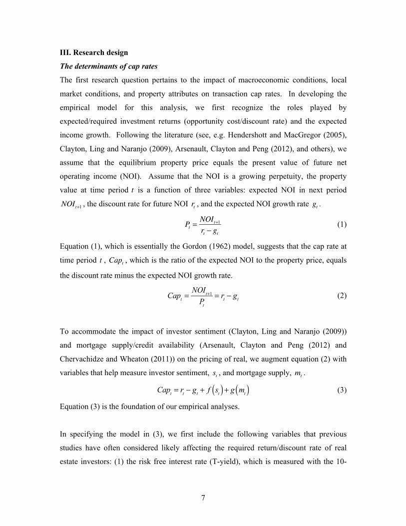
The first research question pertains to the impact of macroeconomic conditions, local

market conditions, and property attributes on transaction cap rates. In developing the

empirical model for this analysis, we first recognize the roles played by

expected/required investment returns (opportunity cost/discount rate) and the expected

income growth. Following the literature (see, e.g. Hendershott and MacGregor (2005),

Clayton, Ling and Naranjo (2009), Arsenault, Clayton and Peng (2012), and others), we

assume that the equilibrium property price equals the present value of future net

operating income (NOI). Assume that the NOI is a growing perpetuity, the property

value at time period t is a function of three variables: expected NOI in next period

NOIt+1 , the discount rate for future NOI rt , and the expected NOI growth rate gt .

Pt =NOIt+1rt − gt

(1)

Equation (1), which is essentially the Gordon (1962) model, suggests that the cap rate at

time period t , Capt , which is the ratio of the expected NOI to the property price, equals

the discount rate minus the expected NOI growth rate.

Capt =

NOIt+1

Pt

= rt − gt (2)

To accommodate the impact of investor sentiment (Clayton, Ling and Naranjo (2009))

and mortgage supply/credit availability (Arsenault, Clayton and Peng (2012) and

Chervachidze and Wheaton (2011)) on the pricing of real, we augment equation (2) with

variables that help measure investor sentiment, st , and mortgage supply, mt .

Capt = rt − gt + f st( ) + g mt( ) (3)

Equation (3) is the foundation of our empirical analyses.

In specifying the model in (3), we first include the following variables that previous

studies have often considered likely affecting the required return/discount rate of real

estate investors: (1) the risk free interest rate (T-yield), which is measured with the 10-

8

Year Treasury Constant Maturity Rate; (2) the expected inflation (Term Spread), which is

measured with the difference between the 10-Year and 1-Year Treasury Constant

Maturity Rates; (3) the credit risk (Credit Spread), which is the difference between

Moody's Seasoned AAA Corporate Bond Yield and BAA Corporate Bond Yield; and (4)

stock market factors, which are the Fama-French factors (FF: Rm-Rf, FF: SMB, and FF:

HML).

Furthermore, Arsenault, Clayton and Peng (2012) find that cap rates are significantly

related to recent performance of commercial real estate investments. Particularly, ex post

Jensen’s Alpha estimated from past commercial investment returns and stock market risk

premium significantly reduces cap rates, likely because they reduce the required risk

premium. Following this study, we include in the model in (3) two performance

measurements of commercial real estate investments: ex post Jensen’s Alpha and CAPM

Beta (NPI: Alpha and NPI: Beta) that are jointly estimated from a regression of the

NCREIF Price Index (total return) in the past 8 quarters against an intercept and the stock

market risk premium, which is measured with the Rm-Rf of Fama-French factor in those

quarters. The intercept term is interpreted as the ex post Jensen’s Alpha and the

coefficient of the stock market risk premium is the CAPM Beta.

We investigate three property attributes that are likely affecting cap rates: (1) the age of

the property when traded (Age); the size of the property (Size) when traded, which is

measured with log of thousand gross square feet; and (3) the “class” of the property (Rent

Premium), which is measured with the median of the historical ratio of the rent (dollar

per square foot per quarter) of the property and the median rent in the CBSA for the same

property type in the sample period. The variable Age likely measures a variety of factors.

For example, newer properties may better utilize new technologies and provide more

amenities. However, Age may also be related to the desirability of the location. For

instance, older office buildings tend to be located in more desirable location, as land in

such location tends to be developed earlier. Therefore, the impact of Age on cap rates

can be complicated and may vary across property types. The variable Size might be

related to possible “clientele effects” – larger buildings more likely host larger

9

corporations, which might react differently to economic shocks than smaller companies.

This might translate into different perceptions of income stability, and thus affect

investors’ required returns. The variable Rent Premium is also possibly related to

“clientele effects” – tenants who afford higher rents might be more resilient to economic

shocks and thus rents might be more stable. However, it is important to note that it is

ultimately an empirical question whether these property attributes affect cap rates.

We consider the following macroeconomic variables that likely influence real estate

investors’ expectation of future income growth: (1) the growth of GDP in the previous

quarter (GDP Growth); and (2) the NBER-based recession indicator (Recession).

Regional/local market conditions that might affect investors’ expectation of income

growth include (1) the median occupancy rate of the CBSA where the property is located

(Occupancy); (2) the growth in the occupancy rate in the present quarter (Occupancy

Growth); (3) the rent growth in the present quarter (Rent Growth); and (4) the interaction

between Rent Growth and Occupancy. We use the interaction term to accommodate

possible nonlinear effect of rent growth on the expected future income growth. When the

occupancy rate is higher, the current rent growth is more likely persistent in the future

due to the limited supply of space.

Clayton, Ling and Naranjo (2009) provide evidence that investor sentiment likely affect

real estate pricing. We use the following variables to measure the sentiment, or optimism,

of investors: (1) total private construction spending on nonresidential properties

normalized with GDP (Construction: Nonresidential); (2) the one-quarter lag of the NPI

total return for the property type (NPI Return); (3) total private construction spending on

residential properties normalized with GDP (Construction: Residential); and (4) the one-

quarter lag of the growth rate of the Standard and Poor's National Composite Home Price

Index for the United States (HPI Growth). We include construction spending as it likely

reflects the market expectation of future demand for space, which may or may not be

accurate/rational. Note that even though we categorize construction spending as a

variable measuring sentiment, it might be also related to the require return of investors

and their expected future returns. For example, overbuilding might reduce expected

10

future income growth. We include the lagged NPI total return, as investors might

extrapolate past returns into the future (see Goetzmann, Peng and Yen (2009) for

evidence for such behavior of home buyers). We include residential construction

spending and lagged growth in house price index, as commercial real estate investor

sentiment might be related to residential real estate investor sentiment - Levitin and

Wachter (2012) point out connections between residential and commercial real estate

bubbles. We choose not to include the mortgage flow, which is used in Clayton, Ling

and Naranjo (2009) to measure sentiment, for two reasons. First, it is likely not

exogenous, as mortgage amount is related to values. Second, unreported robustness

checks indicate that mortgage flow has no significant impact on transaction cap rates.

Arsenault, Clayton and Peng (2012) and Chervachidze and Wheaton (2011) find evidence

that mortgage supply/credit availability affects commercial property pricing. Following

Arsenault, Clayton and Peng (2012), we use the development of the CMBS market to

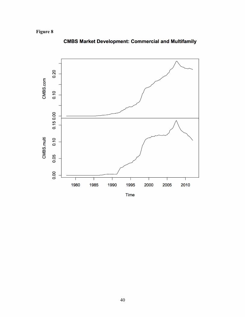
measure the mortgage supply. We measure the CMBS market development for industrial,

office, and retail properties with the ratio of the Federal Flow of Funds Account variable

“Issuers of asset-backed securities; commercial mortgages; asset” to “All sectors;

commercial mortgages; asset”. For apartment, the measurement equals “Issuers of asset-

backed securities; multifamily residential mortgages; asset” divided with “All sectors;

multifamily residential mortgages; asset”. The two measurements are essentially the

percentage of mortgages backed by CMBS. We believe they are superior measurements

of exogenous changes in mortgage supply/credit availability than the total mortgage debt,

as the total mortgage debt is endogenous and jointly determined with property prices.

Finally, time invariant location specific market conditions may affect property cap rates

through their impact on the required returns, expected rent growth, sentiment, and local

credit availability. For example, apartment properties in markets with inelastic land

supply may have lower cap rates, as expected rent growth might be higher with limited

land supply. Such variables are different to measure individually, but it is relatively easy

to control their aggregate effect. We use CBSA dummy variables to capture unobserved

local time invariant variables that affect cap rates.

11

The determinants of cap rate uncertainty

The second research question of this paper is what drives the uncertainty in property cap

rates. While this is a very important question for real estate investors, the literature is

essentially silent on this issue in both theoretical and empirical fronts. This paper aims to

provide initial evidence on this issue.

This paper measures cap rate uncertainty with the magnitude of the component of the cap

rate that is not explained by our model in (3), or more specifically, the squared regression

residuals. We build an empirical model based on the notion that, in a perfect world in

which all factors that affect cap rates have been identified and can be observed for each

individual property, cap rates would be completely explained without residuals, and thus

there is no cap rate uncertainty. Therefore, the uncertainty we measure is primarily

driven by heterogeneity in required returns or expected future income growth, or other

factors, due to the omission of explanatory variables at the national, regional, property,

and transaction level.

Due to the lack of theoretical guidance in searching for the “omitted” variables, we focus

on the possible relationship between the uncertainty in cap rates and the level of cap rates.

We conjecture that investors are risk averse and thus have lower values for properties

with higher risk. Therefore, there might be a positive relationship between the level of

cap rates and the uncertainty in cap rates. To mitigate mechanical relationship between

property cap rates and regression residuals, our analysis measures property values with

the fitted cap rates from estimation of model (3). In this analysis, we include CBSA

dummies to control for risk related to unobserved time invariant local market conditions.

We further control possible effects of property attributes, such as age and size, on cap

rate uncertainty.

IV. Data

Cap rates

12

This paper analyzes actual transaction cap rates of acquisitions and dispositions of the

four main types of institutional grade properties (apartment, industrial, office, and retail)

in the NCREIF database from the third quarter of 1977 to the second quarter of 2012.

We calculate the transaction cap rates for acquisitions and dispositions using similar

approaches with the key difference being the NOI used. For acquisitions, we use the

stabilized annual NOI after the acquisition to calculate cap rates. However, NOI is not

observed after dispositions; therefore, we use the stabilized annual NOI before the

disposition for the cap rate calculation, under the assumption that the NOI after

disposition is proportional in expectation to the NOI before. Our analyses address the

difference in the cap rate definitions for acquisitions and dispositions by including a

dummy variable for dispositions in regressions.

The acquisition cap rates are calculated following the procedure below. First, we identify

acquisitions between 1977:3 and 2012:2 with observed purchase prices (“InitialCost” of

NCREIF database) and transaction time. Second, we identify the quarterly NOI for the

eight quarters (or until the end of the sample period if the acquisition took place within

eight quarters before 2012:2) after each acquisition. For us to proceed with the

calculation of the cap rate, NOI needs to be observed for all the eight quarters; there need

to be at least six quarters that have stabilized NOI, which is defined as NOI when the

occupancy rate (LeasePercent) is above 85%; and the median of the stabilized quarterly

NOI needs to be between 0.5% and 5% of the purchase prices (annual NOI being

between 2% and 20% of the purchase prices). Third, we identify the maximum and the

minimum of the quarterly stabilized NOI, and remove them if they are 50% greater and

less than the median quarterly stabilized NOI. Finally, we calculate the cap rate as four

times the average of the remaining quarterly stabilized NOI, which is intended to capture

the stabilized annual NOI, divided with the purchase prices.

The disposition cap rates are calculated in the same manner, but we use sale prices

(“GrossSalePrice” in NCREIF database) instead of purchase prices, and use the stabilized

NOI before instead of after the disposition. To mitigate possible data errors, we calculate

13

the cap rate for a disposition only if both “GrossSalePrice” and “NetSalePrice” are

observed and their difference is less than 15% of the “NetSalePrice”.

After calculating the acquisition and disposition cap rates, we remove outliers for each

type by excluding the lowest 1% and highest 1% cap rates for each type. Our final

sample consists of 2,891 cap rates (1,608 acquisitions and 1,283 dispositions) for

apartment, 3,113 cap rates (1,961 acquisitions and 1,152 dispositions) for industrial,

2,190 cap rates (1,308 acquisitions 882 dispositions) for office, and 1,832 cap rates

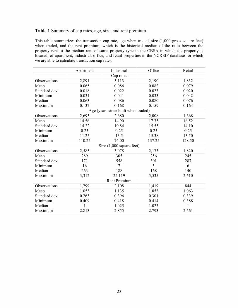
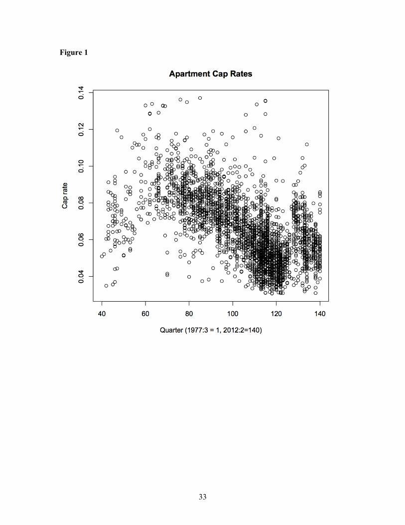
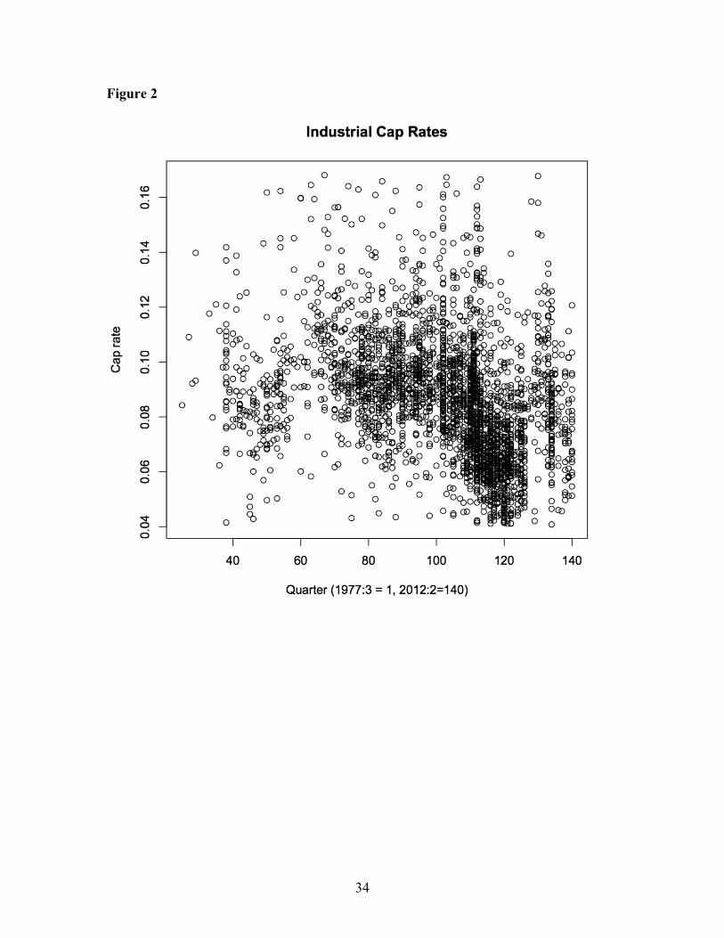
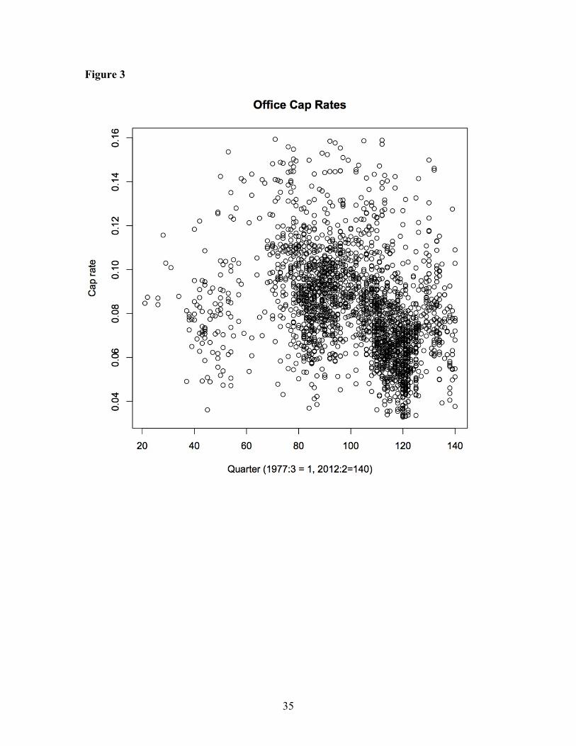
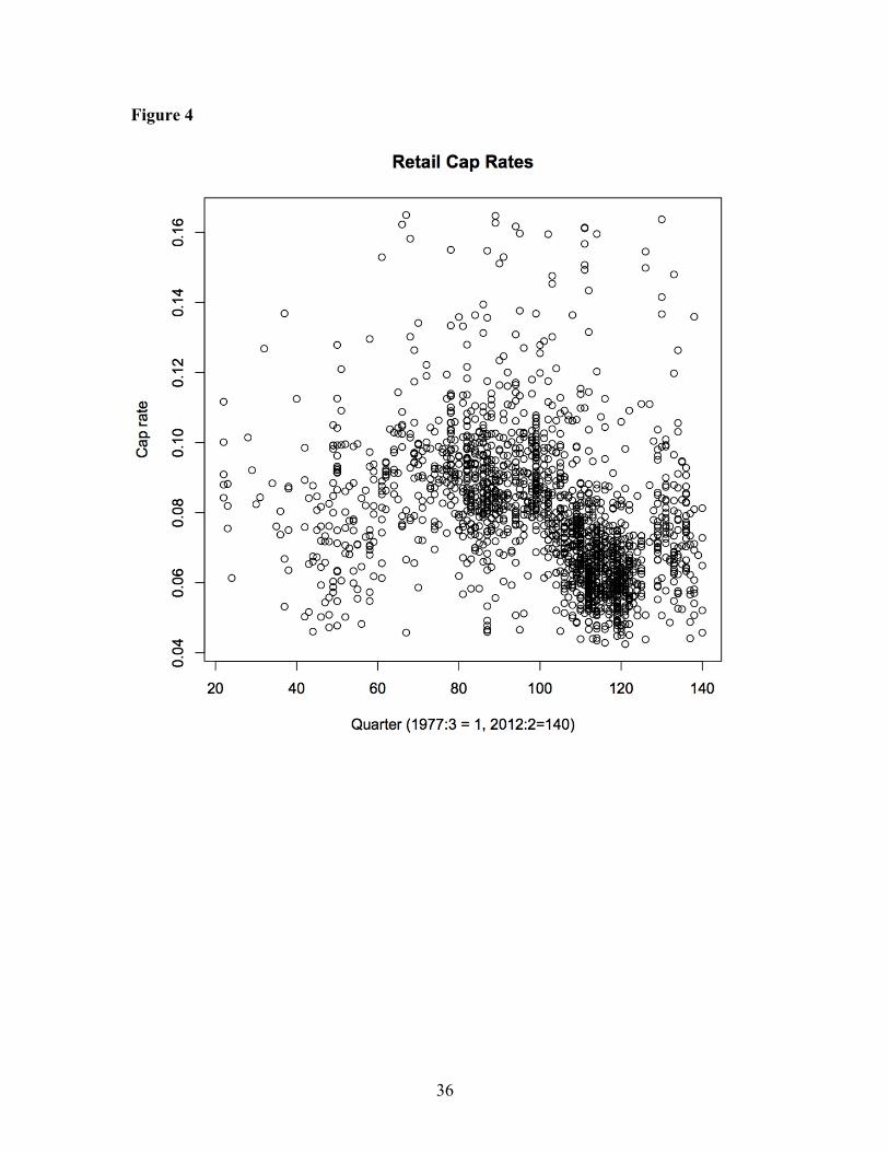
(1,059 acquisitions and 773 dispositions) for retail properties. Table 1 summarizes the

mean, standard deviation, minimum, median, and maximum cap rates for each of the four

property types. Figures 1 to 4 plot the cap rates against the time periods when the

transactions take place for the four property types respectively.

Macro variables

Macro level variables used in our analyses are from four sources: the Federal Reserve

Economic Data (FRED), the Federal Flow of Funds Account, the NCREIF website, and

the data library on the website of Kenneth French.

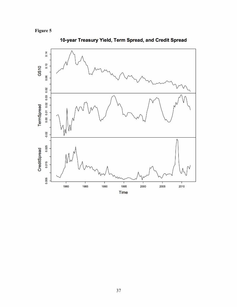
We obtain the following quarterly variables from the FRED: the 10-Year Treasury

Constant Maturity Rate, the term spread (the difference between the 10-Year and 1-Year

Treasury Constant Maturity Rates), the credit spread (the difference between Moody's

Seasoned AAA Corporate Bond Yield and BAA Corporate Bond Yield), the growth rate

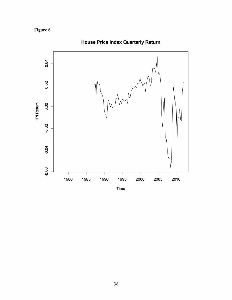
of GDP (GDP being seasonally adjusted annual rate), the Standard and Poor's National

Composite Home Price Index for the United States, NBER-based Recession Indicators,

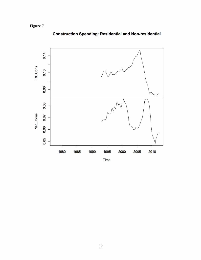
the total private construction spending on residential properties (seasonally adjusted

annual rate), and the total private construction spending on nonresidential properties

(seasonally adjusted annual rate). We normalize the construction spending with the GDP.

Figure 5 plots the time series of the Treasury yield, the term spread, and the credit spread

from 1977:3 to 2012:2. Figures 6 and 7 plot the Home Price Index and the normalized

construction spending for residential and nonresidential properties for this period.

14

We calculate the following quarterly time series using information from the Federal Flow

of Funds Account: the development of the CMBS market for industrial, office, and retail

properties (“Issuers of asset-backed securities; commercial mortgages; asset” divided

with “All sectors; commercial mortgages; asset” for commercial mortgages), the

development of the CMBS market for apartment (“Issuers of asset-backed securities;

multifamily residential mortgages; asset” divided with “All sectors; multifamily

residential mortgages; asset” for multifamily mortgages). The time series of the two

measurements of the CMBS market development are plotted in Figure 8.

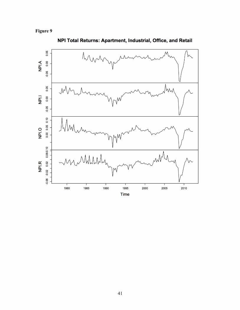
We download the quarterly Fama-French factors – Rm-Rf, SMB, and HML – from

Kenneth French’s website, and the quarterly total returns of NCREIF Price Indices for the

four property types from the website of NCREIF. Figure 9 plots the NPI total returns.

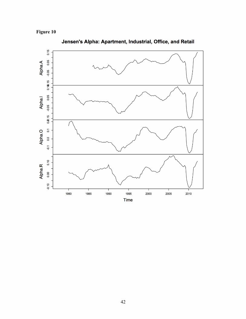
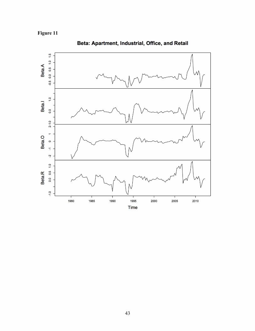
We construct ex post Jensen’s Alpha and CAPM Beta for each property type in each

quarter using the NPI total returns and the stock market risk premium (Rm-Rf of the

Fama-French factors) in the past eight quarters. Specifically, for quarter t , we regress

the NPI total returns in quarters t − 8 to t −1 against an intercept term and the stock

market risk premium in those quarters. The intercept term is the ex post Jensen’s Alpha

and the coefficient of the stock market risk premium is the Beta. Figure 10 and Figure 11

respectively plot the estimated ex post Jensen’s Alpha and the estimated CAPM Beta for

the four property types.

Regional and property-level variables

We calculate the medians of the occupancy rate, rent, and their respective growth rate for

each Core Business Statistic Area (CBSA) for each property type using the NCREIF

database, following the procedure below. We first identify property/quarter observations

with the occupancy rate being observed and greater than 70%. For these property/quarter

observations, we estimate the rent as the gross operating income in that quarter divided

by leased space, which equals the gross square feet times the occupancy rate. For each

CBSA/quarter, if there are at least 6 observations of property occupancy rates or rent in

that CBSA/quarter, we remove possible outliers (2 standard deviations away from the

mean) and then calculate the median occupancy rate or the median rent. To obtain the

15

median growth rate in the occupancy rate and the median growth rate in rents, we used

rents estimated above and the occupancy rate for each property to calculate the growth

rates for each property/quarter. We then eliminate growth rates that are greater 20% or

lower than -20%. If there are at least 6 observations left for that CBSA/quarter, we

remove possible outliers (2 standard deviations away from the mean) and then calculate

the median of the growth rate in occupancy rate and the median in rent growth.

The NCREIF database often contains “YearBuilt” for properties, which is used to

calculate the property age (age being in quarters with the quarter of being built assumed

to be the 2nd quarter of the year when the property was built) when a transaction takes

place. The NCREIF database also often contains information on property size. We use

“GrossSquareFeet” to measure property size, if this information is available and the value

is greater than 5,000 square feet (values lower than 5,000 could be data errors or indicate

properties that are too small). If the value of “GrossSquareFeet” changes over time for a

property, we use the available value of the quarter that is closest to the transaction date.

We also calculate the “rent premium” for each property whenever possible. We first

calculate the property-to-market rent ratio for each quarter that allows such a calculation.

Given the time series of such a ratio, which may contain internal missing information, we

calculate the median of the observed ratios. Summary statistics of Age, Size, and Rent

Premium are reported in Table 1.

V. Empirical results

Determinants of cap rates

It is important to note that there is the well-known “clustering” problem in all of our

regressions in this paper. There could be unobserved common shocks for all properties in

the same quarter, or for all properties in the same CBSA when CBSA dummies are not

included. To mitigate the impact of the unobserved common shocks on the calculation of

the standard deviation (see, e.g. Petersen (2009) for the importance of the correction to

the OLS standard deviation), in all reported results, we calculate one-way (sale quarter)

clustering-robust standard deviations when CBSA dummies are included, and two-way

16

(quarter and CBSA) clustering-robust standard deviations when CBSA dummies are not

included.2

In estimating the model in equation (3), we first include only macroeconomic variables

and run OLS for each property type separately. The reason is that, while all cap rate

observations have corresponding macroeconomic variables, CBSA level or property level

variables are sometimes missing. Using macroeconomic variables only will allow us to

investigate the impact of such variables using the full sample.

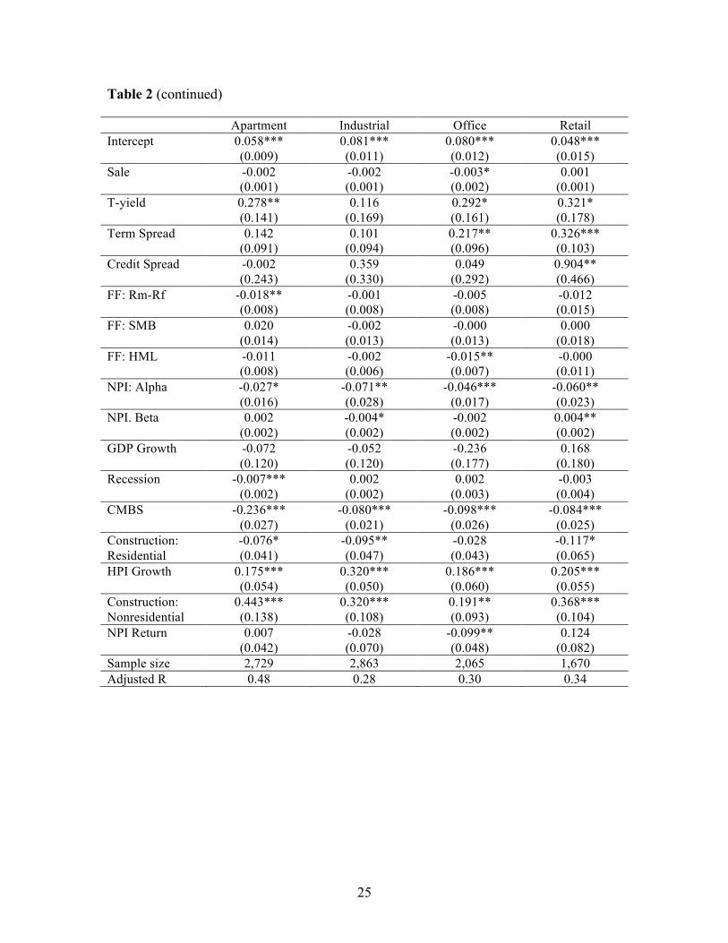
Table 2 reports the results for each property type. Four variables – the ex post Jensen’s

Alpha, the development of the CMBS market, the lagged house price index appreciation,

and the construction spending on nonresidential properties – show statistically significant

explanatory power for cap rates for all four property types. Specifically, the higher is the

ex post Jensen’s Alpha, the lower is the cap rate. This is consistent with Arsenault,

Clayton and Peng (2012). Further, the more developed is the CMBS, which indicates

greater credit availability, the lower is the cap rate. This corroborates Arsenault, Clayton

and Peng (2012) and Chervachidze and Wheaton (2011). It is interesting to see that

higher lagged house price index appreciation and more nonresidential construction

spending seem bad news for property pricing. The negative impact of construction on

property values may indicate that investors reduce their expectation for future income

growth when they expect an increase in space supply. It is worth noting that other

macroeconomic variables, including the term spread, the credit spread, the stock market

factors, and investor sentiment as measured with the lagged NPI total return, do not show

consistent effects on cap rates across property types.

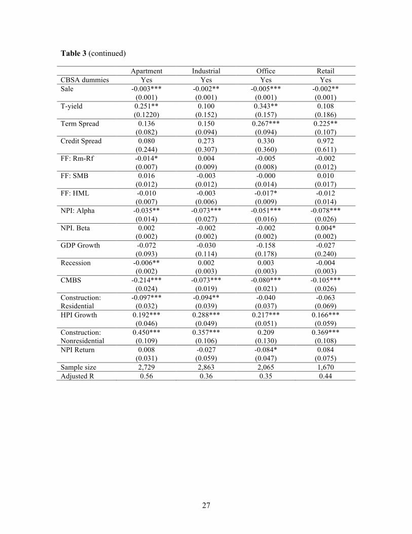
Table 3 reports results from similar regressions, with the only difference being that the

regressions include CBSA dummy variables to capture CBSA specific average cap rates

(CBSA fixed effects). Two results are worth noting. First, it is clear that including

CBSA fixed effects dramatically increase the explanatory power of our model. The

adjusted R2 increases from 0.48 to 0.56 for apartment, from 0.28 to 0.36 for industrial,

2 The R functions we use are from Mahmood Arai’s website.

17

from 0.30 to 0.35 for office, and from 0.36 to 0.44 for retail properties. Second, the four

most influential macroeconomic variables remain significant, except that the

nonresidential construction spending now has insignificant impact on office cap rates.

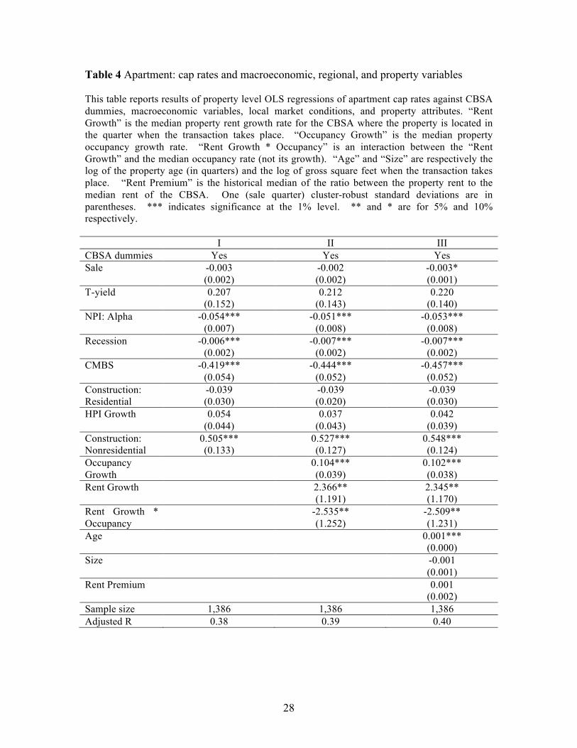
Tables 4 report results of three regressions of cap rates for apartment, all of which include

CBSA dummies. The first regression includes macroeconomic variables that are

significant at 5% level in Table 3 for apartment. The second includes both these

macroeconomic variables and local time varying market variables. The third includes

these macroeconomic variables, local market conditions, and property attributes. For

each property type, we use the same sample for the three regressions. The sample

consists of cap rate observations that have explanatory variables in all three regressions

observed. A disadvantage of using these “complete” observations is the smaller sample

size. An advantage is that when we run the three types of regressions using the same

sample, any gain in goodness of fit is not likely due to a larger sample size, but due to the

inclusion of new independent variables.

Table 4 provides a few important findings. First, local time varying market conditions

and property attributes add very little to the goodness of fit. The adjusted R-square is

0.38, 0.39, and 0.40 for the three regressions respectively, which means including local

market conditions and property attributes does not explain much of the cap rates. Second,

in addition to ex post Jensen’s Alpha, the development of the CMBS market, and the

nonresidential construction spending, the NBER-based recession dummy has a significant

negative effect on the cap rate. This seems to indicate that apartments have relatively

higher values in recessions. This is consistent with that households more likely rent than

own in recessions; therefore, the demand for apartment is higher and thus apartments

might have higher expected future income growth. Third, the lagged house price index

appreciation is no longer significant, likely due to the smaller sample size. Fourth, rent

growth rate has a nonlinear relationship with the cap rate. Rent growth rate has greater

negative impact on the cap rate, which means positive effect on the property value, when

the occupancy rate is higher. Finally, older apartment buildings tend to have higher cap

rates, possibly due to outdated amenities.

18

Table 5 reports the same three regressions, but for industrial properties. The

macroeconomic variables included are those significant for industrial in Table 3. All

three regressions are also based on the same sample of “complete” observations. Table 5

indicates that the four key macroeconomic variables – ex post Jensen’s Alpha, the CMBS

development, the lagged house price index appreciation, and the construction spending of

nonresidential properties – remain significant. Moreover, the construction spending of

residential properties is also significant, and has a negative coefficient. This seems to

suggest that a better prospect of the housing market, which is indicated by the greater

construction spending, is good news for values of industrial properties. This seems

consistent with Miller, Peng and Sklarz (2011), which provide evidence that house

transaction volume, which predicts higher house prices in the future, stimulates economic

production. Table 5 also indicates the same nonlinear impact of rent growth on cap rates.

However, now rent growth seems less effective when the occupancy is high. This seems

puzzling, and contrasts with the results for apartment. Finally, property attributes

contribute modestly to the explanatory power of the model. The adjusted R-square

increased from 0.38 to 0.43 when property age, size, and rent premium are included as

explanatory variables. Table 5 shows that larger and lower class (lower rent premium)

industrial properties tend to have lower cap rates.

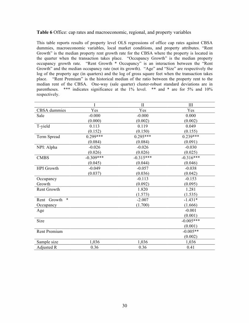
Table 6 reports results of the same three regressions based on “complete” observations

for office properties. First, while the CMBS development remain significant, Jensen’s

Alpha and lagged house price index appreciation are no longer significant, possibly due

to the smaller sample size. Second, the term spread has a significant positive impact on

office cap rates. This is consistent with the notion that, when the expected inflation is

high, office investors requires higher returns. Third, older and larger office properties

tend to have lower cap rates, likely because they have more desirable location, but

alternative explanations cannot be ruled out.

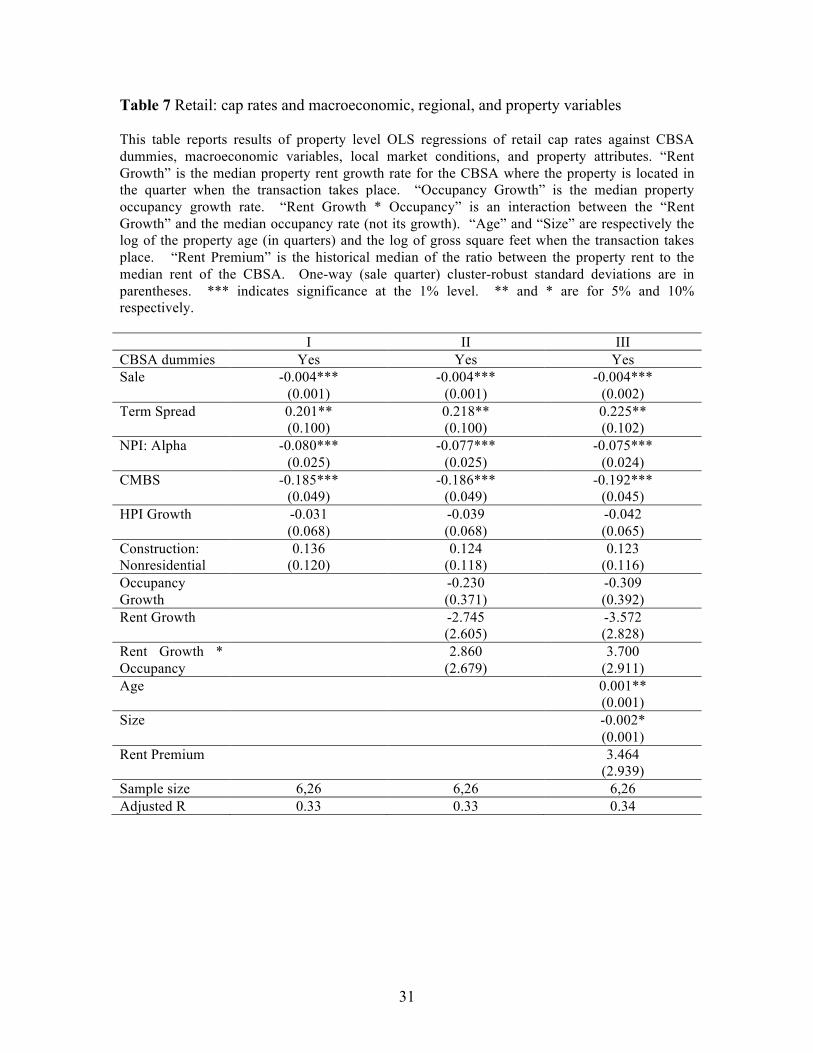
Results of the same three regressions based on “complete” observations for retail

properties are reported in Table 7. Note that the ex post Jensen’s Alpha, the lagged house

19

price index appreciation, and the construction spending of nonresidential properties are

no longer significant. It is also interesting to note that rent growth has no detectable

impact on the cap rate. Finally, both age and size affect cap rates – younger and larger

retail properties tend to have lower cap rates.

We also conduct a few alternative analyses using different measurements of

macroeconomic variables and local market conditions, such as the level of occupancy

rate instead of/in addition to the change of the occupancy rate. These alternative

specifications do not change the main findings reported above, and do not provide better

explanation of property cap rates.

Determinants of cap rate uncertainty

The second part of our empirical analysis is the determinants of the uncertainty in cap

rates, which we measure with squared residuals from the regressions in Table 3. Note

that regressions in Table 3 include CBSA dummies and macroeconomic variables, but

not local market conditions or property attributes. We use residuals from Table 3 instead

of residuals from some regressions in Tables 4 to 7 for two reasons. First, as Tables 4 to

7 indicate, local market conditions and property attributes tend to add modest or little

explanatory power for cap rates. Omitting them does not have meaningful impact on the

residuals. Second, using residuals from Table 2 allows us to maintain a larger sample

size, and gives our analysis more power.

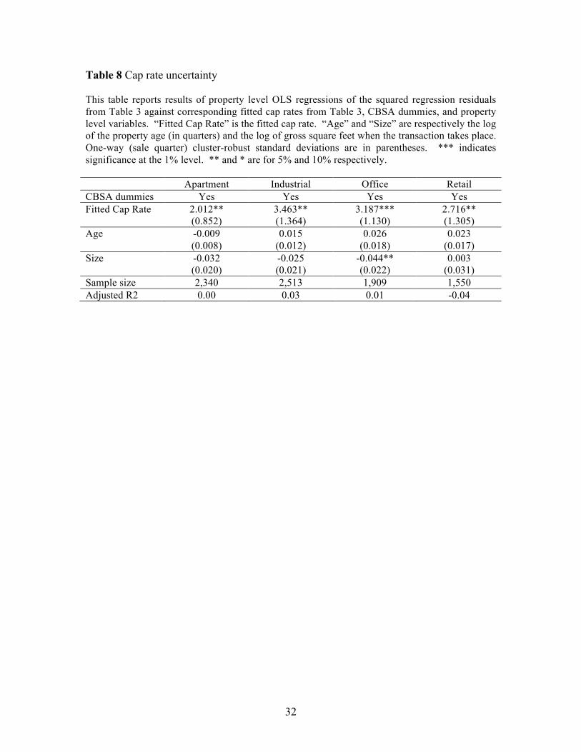
Table 8 reports results of OLS regressions of squared residuals on CBSA dummy

variables, the corresponding fitted values of cap rates, which are from the same

regressions that generate the residuals, as well as the age and the size of properties. Rent

premium is not significant in robustness checks so we do not include it as an explanatory

variable. Since age and size information is sometimes missing, the sample size in Table

8 is smaller than the sample size in Table 3.

Table 8 provides three interesting results. First, the higher is the fitted cap rate, the lower

is the uncertainty in cap rate. This relationship is statistically significant for all properties,

20

and is consistent with the conjecture that investors have higher values for properties with

lower pricing risk. Second, age and size has virtually no relationship with uncertainty in

cap rates, except that larger offices have less cap rate uncertainty. Third, the adjusted R2

is virtually 0 in all regressions. This calls for more theoretical and empirical work on the

determinants of cap rate uncertainty.

VI. Conclusions

Better understanding of the determinants of cap rates of commercial properties is crucial

for economists. Asset pricing is a central question in economics and finance, and the

pricing of large, heterogeneous, and not dividable assets such as commercial properties is

challenging and important given the large size of commercial properties in the economy.

The knowledge on the determinants of property cap rates is also essential for investors to

make provident acquisition and disposition decisions. For example, a slight change in a

going-out cap rate could dramatically affect the valuation of a target of acquisition, and

lead to very different decisions.

This paper makes two important contributions to our understanding of commercial real

estate pricing. First, it provides novel evidence regarding how cap rates of individual

properties are affected by macroeconomic conditions, local market conditions, and

property attributes. It finds that CBSA fixed effects and macroeconomic conditions,

particularly the ex post Jensen’s Alpha, the credit availability, the lagged house price

appreciation, and the nonresidential construction spending, play a dominating role in

explaining cap rates. It finds weak explanatory power of local market conditions and

property attributes, the effects of which vary across property types.

Second, this paper provides an original finding regarding the determinants of uncertainty

in cap rates. Specifically, there is positive relationship between uncertainty in cap rates

and the level of cap rates, which seem to indicate that investors pay more for properties

with less pricing risk.

21

References

Ambrose, B., and H.O. Nourse, 1993, Factors influencing capitalization rates, Journal of Real Estate Research 8, 221-237.

An, Xudong, and Yongheng Deng, 2009, A structural model for capitalization rate, San Diego State University Working Paper.

Arsenault, Marcel, Jim Clayton, and Liang Peng, 2012, Mortgage fund flows, capital appreciation, and real estate cycles, Journal of Real Estate Finance and Economics DOI: 10.1007/s11146-012-9361-4.

Chervachidze, Serguei, and William Wheaton, 2011, What determined the great cap rate compression of 2000–2007, and the dramatic reversal during the 2008–2009 financial crisis?, Journal of Real Estate Finance and Economics DOI 10.1007/s11146-011-9334-z.

Chichernea, Doina, Norman G. Miller, Jeffrey D. Fisher, Bob White, and Michael Sklarz, 2008, A cross-sectional analysis of cap rates by msa, Journal of Real Estate Research 30.

Clayton, Jim, David Ling, and Andy Naranjo, 2009, Commercial real estate valuation: Fundamentals versus investor sentiment, Journal of Real Estate Finance and Economics 38, 5-37.

Elliehausen, Gregory, and Joseph B. Nichols, 2012, Determinants of capitalization rates for office properties, Federal Reserve Board working paper.

Evans, R., 1990, A transfer function analysis of real estate capitalization rates, Journal of Real Estate Research 5, 371-379.

Froland, C, 1987, What determines cap rates on real estate, Journal of Portfolio Management 13, 77-83.

Goetzmann, William N., Liang Peng , and Jacqueline Yen, 2009, The subprime crisis and house price appreciation, Yale ICF Working Paper No. 1340577 Available at SSRN: http://ssrn.com/abstract=1340577.

Gordon, Myron J., 1962, The investment, financing, and valuation of the corporation, Homewood, Illinois: Richard D. Irwin, Inc.

Hendershott, P. H., and B. D. MacGregor, 2005, Investors rationality: Evidence from u.K. Property capitalization rates, Real Estate Economics 33, 299-322.

Jud, D., and D. Winkler, 1995, The capitalization rate of commercial properties and market returns, Journal of Real Estate Research 10: 509-518 10, 509-518.

Levitin, Adam J., and Susan M. Wachter, 2012, The commercial real estate bubble, Business, Economics, and Regulatory Policy Working Paper Series No. 1978264.

Miller, Norman, Liang Peng, and Michael Sklarz, 2011, Economic impact of anticipated house price changes - evidence from home sales, Real Estate Economics 39, 345-378.

Peng, Liang, 2012, Risk and returns of commercial real estate: A property level analysis, Available at SSRN: http://ssrn.com/abstract=1658265.

Peng, Liang, and Thomas Thibodeau, 2012, Risk segmentation of american homes: Evidence from denver, Real Estate Economics forthcoming.

Petersen, Mitchell A., 2009, Estimating standard errors in finance panel data sets: Comparing approaches, Review of Financial Studies 22, 435-480.

Pivo, Gary, and Jeffrey D. Fisher, 2011, The walkability premium in commercial real estate investments, Real Estate Economics 39.

22

Plazzi, Alberto, Walter Torous, and Rossen Valkanov, 2008, The cross-sectional dispersion of commercial real estate returns and rent growth: Time variation and economic flucuations, Real Estate Economics 36, 403-439.

Plazzi, Alberto, Walter Torous, and Rossen Valkanov, 2010, Expected returns and the expected growth in rents of commercial real estate, Review of Financial Studies 23, 3469-3519.

Sivitanides, P., J. Southard, R. Torto, and W. Wheaton, 2001, The determinants of appraisal-based capitalization rates, Real Estate Finance 18, 27-37.

Sivitanidou, R., and P. Sivitanides, 1999, Office capitalization rates: Real estate and capital market influences, Journal of Real Estate Finance and Economics 18, 297-322.

Wiley, Jonathan A., 2013, Buy high, sell low: Corporate investors in the office market, Real Estate Economics 41.

23

Table 1 Summary of cap rates, age, size, and rent premium This table summarizes the transaction cap rate, age when traded, size (1,000 gross square feet) when traded, and the rent premium, which is the historical median of the ratio between the property rent to the median rent of same property type in the CBSA in which the property is located, of apartment, industrial, office, and retail properties in the NCREIF database for which we are able to calculate transaction cap rates. Apartment Industrial Office Retail

Cap rates Observations 2,891 3,113 2,190 1,832 Mean 0.065 0.086 0.082 0.079 Standard dev. 0.018 0.022 0.023 0.020 Minimum 0.031 0.041 0.033 0.042 Median 0.063 0.086 0.080 0.076 Maximum 0.137 0.168 0.159 0.164

Age (years since built when traded) Observations 2,695 2,680 2,008 1,668 Mean 14.56 14.90 17.75 16.52 Standard dev. 14.22 10.84 15.55 14.10 Minimum 0.25 0.25 0.25 0.25 Median 11.25 13.5 15.38 13.50 Maximum 110.25 76.00 137.25 128.50

Size (1,000 square feet) Observations 2,585 3,078 2,173 1,820 Mean 289 305 256 245 Standard dev. 171 558 301 287 Minimum 16 7 5 6 Median 263 188 168 140 Maximum 3,312 22,119 5,535 2,610

Rent Premium Observations 1,799 2,108 1,419 844 Mean 1.053 1.135 1.053 1.063 Standard dev. 0.263 0.396 0.301 0.339 Minimum 0.409 0.418 0.414 0.388 Median 1 1.025 1.023 1 Maximum 2.813 2.855 2.793 2.661

24

Table 2 Cap rates and macro variables This table reports results of property level OLS regressions of cap rates against macro-level variables. “Sale” is a dummy variable if the cap rate is for a disposition. “T-yield” is the 10-Year Treasury Constant Maturity Rate. “Term Spread” is the difference between the 10-Year and 1-Year Treasury Constant Maturity Rates. “Credit Spread” is the difference between Moody's Seasoned AAA Corporate Bond Yield and BAA Corporate Bond Yield. “FF: Rm-Rf”, “FF: SMB”, and “FF: HML” are the Fama-French factors. “NPI: Alpha” and “NPI: Beta” are ex post Jensen’s Alpha and CAPM Beta estimated using the NPI property type total returns and the “FF: Rm-Rf” in the past 8 quarters. “GDP Growth” is one-quarter lag of the growth rate of GDP. “Recession” is the NBER-based recession indicator. “CMBS” is the development of the CMBS market, which equals “Issuers of asset-backed securities; commercial mortgages; asset” divided with “All sectors; commercial mortgages; asset” for industrial, office, and retail properties, and equals “Issuers of asset-backed securities; multifamily residential mortgages; asset” divided with “All sectors; multifamily residential mortgages; asset” for apartment. “Construction: Residential” is the total private construction spending on residential properties normalized with GDP. “HPI growth” is the one-quarter lag of the growth rate of the Standard and Poor's National Composite Home Price Index for the United States. “Construction: Nonresidential” is the total private construction spending on nonresidential properties normalized with GDP. “NPI return” is the one-quarter lag total return of the property type NPI. Two-way (CBSA and sale quarter) cluster-robust standard deviations are in parentheses. *** indicates significance at the 1% level. ** and * are for 5% and 10% respectively.

25

Table 2 (continued)

Apartment Industrial Office Retail Intercept 0.058***

(0.009) 0.081*** (0.011)

0.080*** (0.012)

0.048*** (0.015)

Sale -0.002 (0.001)

-0.002 (0.001)

-0.003* (0.002)

0.001 (0.001)

T-yield 0.278** (0.141)

0.116 (0.169)

0.292* (0.161)

0.321* (0.178)

Term Spread 0.142 (0.091)

0.101 (0.094)

0.217** (0.096)

0.326*** (0.103)

Credit Spread -0.002 (0.243)

0.359 (0.330)

0.049 (0.292)

0.904** (0.466)

FF: Rm-Rf -0.018** (0.008)

-0.001 (0.008)

-0.005 (0.008)

-0.012 (0.015)

FF: SMB 0.020 (0.014)

-0.002 (0.013)

-0.000 (0.013)

0.000 (0.018)

FF: HML -0.011 (0.008)

-0.002 (0.006)

-0.015** (0.007)

-0.000 (0.011)

NPI: Alpha -0.027* (0.016)

-0.071** (0.028)

-0.046*** (0.017)

-0.060** (0.023)

NPI. Beta 0.002 (0.002)

-0.004* (0.002)

-0.002 (0.002)

0.004** (0.002)

GDP Growth -0.072 (0.120)

-0.052 (0.120)

-0.236 (0.177)

0.168 (0.180)

Recession -0.007*** (0.002)

0.002 (0.002)

0.002 (0.003)

-0.003 (0.004)

CMBS -0.236*** (0.027)

-0.080*** (0.021)

-0.098*** (0.026)

-0.084*** (0.025)

Construction: Residential

-0.076* (0.041)

-0.095** (0.047)

-0.028 (0.043)

-0.117* (0.065)

HPI Growth 0.175*** (0.054)

0.320*** (0.050)

0.186*** (0.060)

0.205*** (0.055)

Construction: Nonresidential

0.443*** (0.138)

0.320*** (0.108)

0.191** (0.093)

0.368*** (0.104)

NPI Return 0.007 (0.042)

-0.028 (0.070)

-0.099** (0.048)

0.124 (0.082)

Sample size 2,729 2,863 2,065 1,670 Adjusted R 0.48 0.28 0.30 0.34

26

Table 3 Cap rates, CBSA fixed effect, and macro variables This table reports results of property level OLS regressions of cap rates against dummy variables of CBSAs where properties are located and macro-level variables. “Sale” is a dummy variable if the cap rate is for a disposition. “T-yield” is the 10-Year Treasury Constant Maturity Rate. “Term Spread” is the difference between the 10-Year and 1-Year Treasury Constant Maturity Rates. “Credit Spread” is the difference between Moody's Seasoned AAA Corporate Bond Yield and BAA Corporate Bond Yield. “FF: Rm-Rf”, “FF: SMB”, and “FF: HML” are the Fama-French factors. “NPI: Alpha” and “NPI: Beta” are ex post Jensen’s Alpha and CAPM Beta estimated using the NPI property type total returns and the “FF: Rm-Rf” in the past 8 quarters. “GDP Growth” is one-quarter lag of the growth rate of GDP. “Recession” is the NBER-based recession indicator. “CMBS” is the development of the CMBS market, which equals “Issuers of asset-backed securities; commercial mortgages; asset” divided with “All sectors; commercial mortgages; asset” for industrial, office, and retail properties, and equals “Issuers of asset-backed securities; multifamily residential mortgages; asset” divided with “All sectors; multifamily residential mortgages; asset” for apartment. “Construction: Residential” is the total private construction spending on residential properties normalized with GDP. “HPI growth” is the one-quarter lag of the growth rate of the Standard and Poor's National Composite Home Price Index for the United States. “Construction: Nonresidential” is the total private construction spending on nonresidential properties normalized with GDP. “NPI return” is the one-quarter lag total return of the property type NPI. One-way (sale quarter) cluster-robust standard deviations are in parentheses. *** indicates significance at the 1% level. ** and * are for 5% and 10% respectively.

27

Table 3 (continued)

Apartment Industrial Office Retail CBSA dummies Yes Yes Yes Yes Sale -0.003***

(0.001) -0.002** (0.001)

-0.005*** (0.001)

-0.002** (0.001)

T-yield 0.251** (0.1220)

0.100 (0.152)

0.343** (0.157)

0.108 (0.186)

Term Spread 0.136 (0.082)

0.150 (0.094)

0.267*** (0.094)

0.225** (0.107)

Credit Spread 0.080 (0.244)

0.273 (0.307)

0.330 (0.360)

0.972 (0.611)

FF: Rm-Rf -0.014* (0.007)

0.004 (0.009)

-0.005 (0.008)

-0.002 (0.012)

FF: SMB 0.016 (0.012)

-0.003 (0.012)

-0.000 (0.014)

0.010 (0.017)

FF: HML -0.010 (0.007)

-0.003 (0.006)

-0.017* (0.009)

-0.012 (0.014)

NPI: Alpha -0.035** (0.014)

-0.073*** (0.027)

-0.051*** (0.016)

-0.078*** (0.026)

NPI. Beta 0.002 (0.002)

-0.002 (0.002)

-0.002 (0.002)

0.004* (0.002)

GDP Growth -0.072 (0.093)

-0.030 (0.114)

-0.158 (0.178)

-0.027 (0.240)

Recession -0.006** (0.002)

0.002 (0.003)

0.003 (0.003)

-0.004 (0.003)

CMBS -0.214*** (0.024)

-0.073*** (0.019)

-0.080*** (0.021)

-0.105*** (0.026)

Construction: Residential

-0.097*** (0.032)

-0.094** (0.039)

-0.040 (0.037)

-0.063 (0.069)

HPI Growth 0.192*** (0.046)

0.288*** (0.049)

0.217*** (0.051)

0.166*** (0.059)

Construction: Nonresidential

0.450*** (0.109)

0.357*** (0.106)

0.209 (0.130)

0.369*** (0.108)

NPI Return 0.008 (0.031)

-0.027 (0.059)

-0.084* (0.047)

0.084 (0.075)

Sample size 2,729 2,863 2,065 1,670 Adjusted R 0.56 0.36 0.35 0.44

28

Table 4 Apartment: cap rates and macroeconomic, regional, and property variables This table reports results of property level OLS regressions of apartment cap rates against CBSA dummies, macroeconomic variables, local market conditions, and property attributes. “Rent Growth” is the median property rent growth rate for the CBSA where the property is located in the quarter when the transaction takes place. “Occupancy Growth” is the median property occupancy growth rate. “Rent Growth * Occupancy” is an interaction between the “Rent Growth” and the median occupancy rate (not its growth). “Age” and “Size” are respectively the log of the property age (in quarters) and the log of gross square feet when the transaction takes place. “Rent Premium” is the historical median of the ratio between the property rent to the median rent of the CBSA. One (sale quarter) cluster-robust standard deviations are in parentheses. *** indicates significance at the 1% level. ** and * are for 5% and 10% respectively. I II III CBSA dummies Yes Yes Yes Sale -0.003

(0.002) -0.002 (0.002)

-0.003* (0.001)

T-yield 0.207 (0.152)

0.212 (0.143)

0.220 (0.140)

NPI: Alpha -0.054*** (0.007)

-0.051*** (0.008)

-0.053*** (0.008)

Recession -0.006*** (0.002)

-0.007*** (0.002)

-0.007*** (0.002)

CMBS -0.419*** (0.054)

-0.444*** (0.052)

-0.457*** (0.052)

Construction: Residential

-0.039 (0.030)

-0.039 (0.020)

-0.039 (0.030)

HPI Growth 0.054 (0.044)

0.037 (0.043)

0.042 (0.039)

Construction: Nonresidential

0.505*** (0.133)

0.527*** (0.127)

0.548*** (0.124)

Occupancy Growth

0.104*** (0.039)

0.102*** (0.038)

Rent Growth 2.366** (1.191)

2.345** (1.170)

Rent Growth * Occupancy

-2.535** (1.252)

-2.509** (1.231)

Age 0.001*** (0.000)

Size -0.001 (0.001)

Rent Premium 0.001 (0.002)

Sample size 1,386 1,386 1,386 Adjusted R 0.38 0.39 0.40

29

Table 5 Industrial: cap rates and macroeconomic, regional, and property variables This table reports results of property level OLS regressions of industrial cap rates against CBSA dummies, macroeconomic variables, local market conditions, and property attributes. “Rent Growth” is the median property rent growth rate for the CBSA where the property is located in the quarter when the transaction takes place. “Occupancy Growth” is the median property occupancy growth rate. “Rent Growth * Occupancy” is an interaction between the “Rent Growth” and the median occupancy rate (not its growth). “Age” and “Size” are respectively the log of the property age (in quarters) and the log of gross square feet when the transaction takes place. “Rent Premium” is the historical median of the ratio between the property rent to the median rent of the CBSA. One-way (sale quarter) cluster-robust standard deviations are in parentheses. *** indicates significance at the 1% level. ** and * are for 5% and 10% respectively. I II III CBSA dummies Yes Yes Yes Sale -0.000

(0.001) -0.000 (0.000)

0.000 (0.001)

NPI: Alpha -0.097*** (0.020)

-0.098*** (0.021)

-0.094*** (0.020)

CMBS -0.177*** (0.038)

-0.170*** (0.039)

-0.193*** (0.039)

Construction: Residential

-0.072** (0.031)

-0.068** (0.031)

-0.075** (0.034)

HPI Growth 0.187*** (0.061)

0.190*** (0.061)

0.186*** (0.066)

Construction: Nonresidential

0.413*** (0.096)

0.411*** (0.099)

0.413*** (0.103)

Occupancy Growth

-0.395 (1.319)

-0.562 (1.304)

Rent Growth -12.168*** (3.210)

-13.178*** (3.329)

Rent Growth * Occupancy

12.255*** (3.268)

13.284*** (3.388)

Age 0.001 (0.000)

Size -0.003*** (0.001)

Rent Premium 0.006*** (0.001)

Sample size 1,550 1,550 1,550 Adjusted R 0.38 0.39 0.43

30

Table 6 Office: cap rates and macroeconomic, regional, and property variables This table reports results of property level OLS regressions of office cap rates against CBSA dummies, macroeconomic variables, local market conditions, and property attributes. “Rent Growth” is the median property rent growth rate for the CBSA where the property is located in the quarter when the transaction takes place. “Occupancy Growth” is the median property occupancy growth rate. “Rent Growth * Occupancy” is an interaction between the “Rent Growth” and the median occupancy rate (not its growth). “Age” and “Size” are respectively the log of the property age (in quarters) and the log of gross square feet when the transaction takes place. “Rent Premium” is the historical median of the ratio between the property rent to the median rent of the CBSA. One-way (sale quarter) cluster-robust standard deviations are in parentheses. *** indicates significance at the 1% level. ** and * are for 5% and 10% respectively. I II III CBSA dummies Yes Yes Yes Sale -0.000

(0.000) -0.000 (0.002)

0.000 (0.002)

T-yield 0.113 (0.152)

0.119 (0.150)

0.049 (0.155)

Term Spread 0.299*** (0.084)

0.295*** (0.084)

0.239*** (0.091)

NPI: Alpha -0.026 (0.026)

-0.026 (0.026)

-0.030 (0.025)

CMBS -0.309*** (0.045)

-0.315*** (0.044)

-0.316*** (0.046)

HPI Growth -0.049 (0.037)

-0.057 (0.036)

-0.038 (0.042)

Occupancy Growth

-0.113 (0.092)

-0.153 (0.095)

Rent Growth 1.820 (1.573)

1.281 (1.535)

Rent Growth * Occupancy

-2.007 (1.700)

-1.431* (1.666)

Age -0.001 (0.001)

Size -0.005*** (0.001)

Rent Premium -0.005** (0.002)

Sample size 1,036 1,036 1,036 Adjusted R 0.36 0.36 0.41

31

Table 7 Retail: cap rates and macroeconomic, regional, and property variables This table reports results of property level OLS regressions of retail cap rates against CBSA dummies, macroeconomic variables, local market conditions, and property attributes. “Rent Growth” is the median property rent growth rate for the CBSA where the property is located in the quarter when the transaction takes place. “Occupancy Growth” is the median property occupancy growth rate. “Rent Growth * Occupancy” is an interaction between the “Rent Growth” and the median occupancy rate (not its growth). “Age” and “Size” are respectively the log of the property age (in quarters) and the log of gross square feet when the transaction takes place. “Rent Premium” is the historical median of the ratio between the property rent to the median rent of the CBSA. One-way (sale quarter) cluster-robust standard deviations are in parentheses. *** indicates significance at the 1% level. ** and * are for 5% and 10% respectively. I II III CBSA dummies Yes Yes Yes Sale -0.004***

(0.001) -0.004***

(0.001) -0.004***

(0.002) Term Spread 0.201**

(0.100) 0.218** (0.100)

0.225** (0.102)

NPI: Alpha -0.080*** (0.025)

-0.077*** (0.025)

-0.075*** (0.024)

CMBS -0.185*** (0.049)

-0.186*** (0.049)

-0.192*** (0.045)

HPI Growth -0.031 (0.068)

-0.039 (0.068)

-0.042 (0.065)

Construction: Nonresidential

0.136 (0.120)

0.124 (0.118)

0.123 (0.116)

Occupancy Growth

-0.230 (0.371)

-0.309 (0.392)

Rent Growth -2.745 (2.605)

-3.572 (2.828)

Rent Growth * Occupancy

2.860 (2.679)

3.700 (2.911)

Age 0.001** (0.001)

Size -0.002* (0.001)

Rent Premium 3.464 (2.939)

Sample size 6,26 6,26 6,26 Adjusted R 0.33 0.33 0.34

32

Table 8 Cap rate uncertainty This table reports results of property level OLS regressions of the squared regression residuals from Table 3 against corresponding fitted cap rates from Table 3, CBSA dummies, and property level variables. “Fitted Cap Rate” is the fitted cap rate. “Age” and “Size” are respectively the log of the property age (in quarters) and the log of gross square feet when the transaction takes place. One-way (sale quarter) cluster-robust standard deviations are in parentheses. *** indicates significance at the 1% level. ** and * are for 5% and 10% respectively. Apartment Industrial Office Retail CBSA dummies Yes Yes Yes Yes Fitted Cap Rate 2.012**

(0.852) 3.463** (1.364)

3.187*** (1.130)

2.716** (1.305)

Age -0.009 (0.008)

0.015 (0.012)

0.026 (0.018)

0.023 (0.017)

Size -0.032 (0.020)

-0.025 (0.021)

-0.044** (0.022)

0.003 (0.031)

Sample size 2,340 2,513 1,909 1,550 Adjusted R2 0.00 0.03 0.01 -0.04

33

Figure 1

34

Figure 2

35

Figure 3

36

Figure 4

37

Figure 5

38

Figure 6

39

Figure 7

40

Figure 8

41

Figure 9

42

Figure 10

43

Figure 11