Fixed Strike Asian Cap/Floor on CMS Rates with Lognormal ...€¦ · Fixed Strike Asian Cap/Floor on CMS Rates with Lognormal Approach July 27, 2011 Issue 1.1 Prepared by ... We adapt

Fixed Strike Asian Cap/Floor on CMS Rateswith Lognormal Approach

July 27, 2011

Issue 1.1

Prepared by

Ling Luo and Anthony Vaz

Issue 1.1

Summary

An analytic pricing methodology has been developed for Asian Cap/Floor with fixed strike rateson CMS rates. The price of an Asian Cap/Floor depends on deal parameters such as reset andpayment structures, CMS rate Tenor and number of average CMS rates; and market data such asdiscount curve, swaption volatility curve, realized CMS rates and correlations between projectedCMS rates.

This pricing methodology can price Vanilla Asian Cap/Floor (with fixed averaging periods), as well asPlain Vanilla Cap/Floor.

CMSOptionLN v1p1.pdf (Ling Luo and Anthony Vaz) Page ii of 14

Issue 1.1

Contents

1 Introduction 1

1.1 Scope . . . . . . . . . . . . . . . . . . . . . . . . . . . . . . . . . . . . . . . . . . . . 1

1.2 Measure Change and Adjustment . . . . . . . . . . . . . . . . . . . . . . . . . . . . . 2

1.3 Future Extensions . . . . . . . . . . . . . . . . . . . . . . . . . . . . . . . . . . . . . 3

2 Background 4

2.1 Notation . . . . . . . . . . . . . . . . . . . . . . . . . . . . . . . . . . . . . . . . . . . 4

2.2 Black Swaption Formula . . . . . . . . . . . . . . . . . . . . . . . . . . . . . . . . . . 4

2.3 Forward Measure . . . . . . . . . . . . . . . . . . . . . . . . . . . . . . . . . . . . . . 6

3 Modelling Swap Rates Under a Common Forward Measure 7

3.1 Changing from Ai Swap Measure to Ti Forward Measure . . . . . . . . . . . . . . . . 7

3.2 Changing from Ti Forward Measure to TP Forward Measure . . . . . . . . . . . . . . 8

4 Analytic Pricing of Fixed Strike CMS Asian Cap/Floor 10

5 Parameter Determination in Analytic Pricing Formula 11

A Black Formula for Lognormal Random Variables 13

References 14

CMSOptionLN v1p1.pdf (Ling Luo and Anthony Vaz) Page iii of 14

Issue 1.1

1 Introduction

1.1 Scope

It is desired to find a valuation formula for an Asian CMS Cap/Floor with a fixed strike rate . A CMS(Constant Maturity Swap) rate is equal to the par swap rate for a swap that starts immediatelyfor a specified tenor. Denote R swap ( t; T,M ) as the forward swap rate determined at time t for aswap starting at time T with a tenor of M years, which implies the swap matures at time T + M .Then the CMS rate with M -year tenor at T can be expressed as R CMS (T,M ) = R swap (T ; T,M ).An Asian CMS Cap is a series of call options or caplets on the average CMS rate observed everyreset over a specified time period. An Asian CMS Floor is a series of put options or floorlets on theaverage CMS rate observed every reset over a specified time period. The average number of CMSrates could be fixed or varying for each caplet/floorlet. A Vanilla Asian Cap/Floor is an AsianCap/Floor with fixed averaging periods for each caplet/floorlet. When the averaging

the Vanilla Asian Cap/Floor becomes a Plain Vanilla Cap/Floor .

The price of a product at time t is the present value of all future cash flows generated bythe product. An Asian CMS Cap/Floor can be decomposed into a series of caplets/floorlets andits price at time t equals to the sum of time t prices of the caplets/floorlets whose payments occurafter t. Denote TP (k), k = 1 , 2, . . . , as the scheduled payment times of a Cap/Floor and V ( t; TP (k))is the time t price of the correponding caplet/floorlet with payment at TP (k), then the price of theCap/Floor at time t is given by

P ( t) =k :TP (k )>t

V ( t; TP (k)) . (1)

The prices of the caplets/floorlets can be calculated independently. For the rest of the document,we focus on the analytic formula for the price of one caplet/floorlet.

Assume N is the average number of CMS rates for a caplet/floorlet and T1, T 2, . . . , T N arethe corresponding reset times, then the option payo at time TP (TP > T N ) for $1 notional is givenas follows

V (TP ) = τP × ω ×1N

N

i=1

R CMS (T i , M ) − K

+

,

where we use the notation [·]+ to mean max ( · , 0), K is the fixed strike rate, ω is the option IDwith ω = 1 for caplets and ω = − 1 for floorlets, T i is the reset time for CMS rate R CMS (T i , M ),and τP denotes the year fraction between payment dates. The value of the payo is unknown untiltime TN and is paid on TP . To compute the value of the option at time t ( t < T P ), we compute anexpectation in the TP forward measure; that is,

V ( t) = P ( t, T P ) × τP × E T P ω ×1N

N

i=1

R CMS (T i , M ) − K

+

F t , t < T P (2)

where P ( t, T P ) is the discount factor between t and TP , E T P {·} denotes the expectation under TPforward measure and F t denotes the information filtration at time t. If t ≥ TN , all the CMS rates

CMSOptionLN v1p1.pdf (Ling Luo and Anthony Vaz) Page 1 of 14

periods arefixed at 1,

Issue 1.1

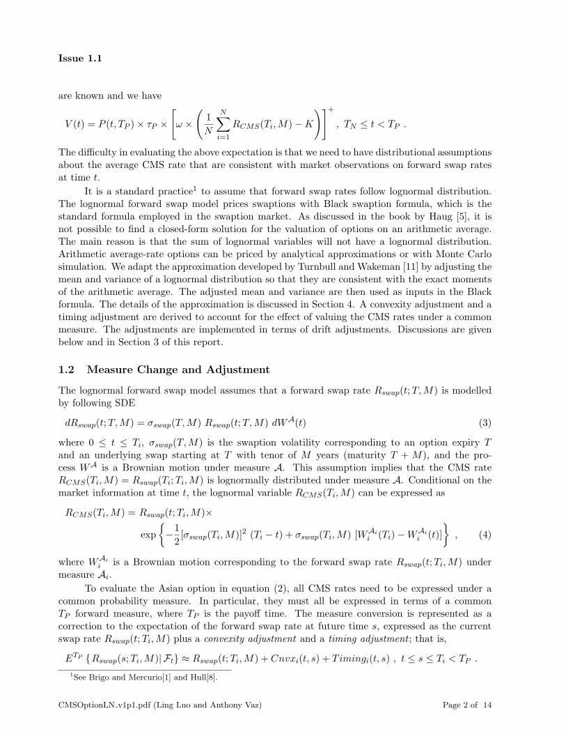
are known and we have

V (t) = P (t, TP )× τP ×

[ω ×

(1

N

N∑i=1

RCMS(Ti,M)−K

)]+, TN ≤ t < TP .

The difficulty in evaluating the above expectation is that we need to have distributional assumptionsabout the average CMS rate that are consistent with market observations on forward swap ratesat time t.

It is a standard practice1 to assume that forward swap rates follow lognormal distribution.The lognormal forward swap model prices swaptions with Black swaption formula, which is thestandard formula employed in the swaption market. As discussed in the book by Haug [5], it isnot possible to find a closed-form solution for the valuation of options on an arithmetic average.The main reason is that the sum of lognormal variables will not have a lognormal distribution.Arithmetic average-rate options can be priced by analytical approximations or with Monte Carlosimulation. We adapt the approximation developed by Turnbull and Wakeman [11] by adjusting themean and variance of a lognormal distribution so that they are consistent with the exact momentsof the arithmetic average. The adjusted mean and variance are then used as inputs in the Blackformula. The details of the approximation is discussed in Section 4. A convexity adjustment and atiming adjustment are derived to account for the effect of valuing the CMS rates under a commonmeasure. The adjustments are implemented in terms of drift adjustments. Discussions are givenbelow and in Section 3 of this report.

1.2 Measure Change and Adjustment

The lognormal forward swap model assumes that a forward swap rate Rswap(t;T,M) is modelledby following SDE

dRswap(t;T,M) = σswap(T,M) Rswap(t;T,M) dWA(t) (3)

where 0 ≤ t ≤ Ti, σswap(T,M) is the swaption volatility corresponding to an option expiry Tand an underlying swap starting at T with tenor of M years (maturity T + M), and the pro-cess WA is a Brownian motion under measure A. This assumption implies that the CMS rateRCMS(Ti,M) = Rswap(Ti;Ti,M) is lognormally distributed under measure A. Conditional on themarket information at time t, the lognormal variable RCMS(Ti,M) can be expressed as

RCMS(Ti,M) = Rswap(t;Ti,M)×

exp

{−1

2[σswap(Ti,M)]2 (Ti − t) + σswap(Ti,M) [WAi

i (Ti)−WAii (t)]

}, (4)

where WAii is a Brownian motion corresponding to the forward swap rate Rswap(t;Ti,M) under

measure Ai.

To evaluate the Asian option in equation (2), all CMS rates need to be expressed under acommon probability measure. In particular, they must all be expressed in terms of a commonTP forward measure, where TP is the payoff time. The measure conversion is represented as acorrection to the expectation of the forward swap rate at future time s, expressed as the currentswap rate Rswap(t;Ti,M) plus a convexity adjustment and a timing adjustment ; that is,

ETP {Rswap(s;Ti,M)| Ft} ≈ Rswap(t;Ti,M) + Cnvxi(t, s) + Timingi(t, s) , t ≤ s ≤ Ti < TP .

1See Brigo and Mercurio[1] and Hull[8].


Issue 1.1

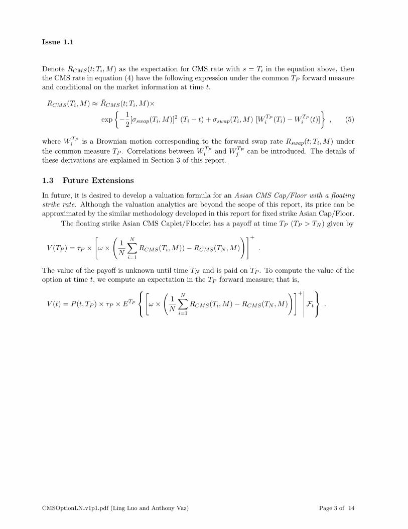
Denote R̄CMS(t;Ti,M) as the expectation for CMS rate with s = Ti in the equation above, thenthe CMS rate in equation (4) have the following expression under the common TP forward measureand conditional on the market information at time t.

RCMS(Ti,M) ≈ R̄CMS(t;Ti,M)×

exp

{−1

2[σswap(Ti,M)]2 (Ti − t) + σswap(Ti,M) [W TP

i (Ti)−W TPi (t)]

}, (5)

where W TPi is a Brownian motion corresponding to the forward swap rate Rswap(t;Ti,M) under

the common measure TP . Correlations between W TPi and W TP

j can be introduced. The details ofthese derivations are explained in Section 3 of this report.

1.3 Future Extensions

In future, it is desired to develop a valuation formula for an Asian CMS Cap/Floor with a floatingstrike rate. Although the valuation analytics are beyond the scope of this report, its price can beapproximated by the similar methodology developed in this report for fixed strike Asian Cap/Floor.

The floating strike Asian CMS Caplet/Floorlet has a payoff at time TP (TP > TN ) given by

V (TP ) = τP ×

[ω ×

(1

N

N∑i=1

RCMS(Ti,M))−RCMS(TN ,M)

)]+.

The value of the payoff is unknown until time TN and is paid on TP . To compute the value of theoption at time t, we compute an expectation in the TP forward measure; that is,

V (t) = P (t, TP )× τP × ETP

[ω ×

(1

N

N∑i=1

RCMS(Ti,M)−RCMS(TN ,M)

)]+∣∣∣∣∣∣Ft

.


Issue 1.1

2 Background

2.1 Notation

Consider a swap that starts at time T0 ≥ 0 and ends at time T0 +M with a tenor of M years, ithas n payments per year at

T1 < . . . < TnM , where TnM = T0 +M .

The first cash flow exchange takes place at T1. A plain vanilla swap contract consists of two legs.One leg pays a floating rate (such as, LIBOR or CDOR) plus a margin spread and the other legpays a fixed rate called the swap rate. The swap rate is determined prior to the start of the swap.Let P (t, T ) be the discount factor between t and T , then the value of the floating leg at time t(t ≤ T0), Vfloat(t), is given by

Vfloat(t) = P (t, T0)− P (t, TnM ).

The value of the fixed leg at time t, Vfixed(t), is given by

Vfixed(t) = Rswap ×nM∑j=1

τjP (t, Tj) ,

where τj is the year fraction between Tj−1 and Tj . The par swap rate is determined so that fixedand floating legs have the same value. Thus the t-time par swap rate is determined as follows:

Rswap(t;T0,M) =P (t, T0)− P (t, TnM )∑nM

j=1 τjP (t, Tj).

The notation Rswap(t;T0,M) indicates that the par swap rate is determined at time t for a swapstarting at time T0 with a tenor of M years, which implies the swap matures at time TnM .

A CMS (constant maturity swap) is a swap contract where one leg pays the M -year swap rate(and possibly plus some margin) while the other leg usually pays a floating rate (such as LIBORor CDOR). The CMS rates are usually set in advance. In particular, the payment on Ti+1 dependson the CMS rate RCMS(Ti,M) which is calculated at Ti for the swap starting at Ti and ending atTi +M , that is, RCMS(Ti,M) = Rswap(Ti;Ti,M).

2.2 Black Swaption Formula

A swaption is an option granting its owner the right, but not the obligation to enter into anunderlying interest rate swap. There are two types of swaption contracts.

1. A payer swaption gives the owner of the swaption the right to enter into a swap, in which hewould pay the fixed leg at the strike rate and receive the floating leg.

2. A receiver swaption gives the owner of the swaption the right to enter into a swap, in whichhe would receive the fixed leg at the strike rate and pay the floating leg.

A swaption is characterized by the following:

1. strike rate (equal to the fixed rate of the underlying swap),


Issue 1.1

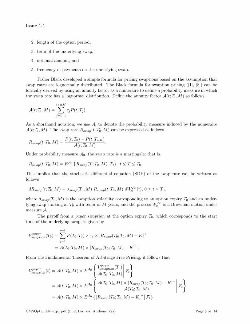
2. length of the option period,

3. term of the underlying swap,

4. notional amount, and

5. frequency of payments on the underlying swap.

Fisher Black developed a simple formula for pricing swaptions based on the assumption thatswap rates are lognormally distributed. The Black formula for swaption pricing ([1], [8]) can beformally derived by using an annuity factor as a numeraire to define a probability measure in whichthe swap rate has a lognormal distribution. Define the annuity factor A(t;Ti,M) as follows.

A(t;Ti,M) =i+nM∑j=i+1

τjP (t, Tj).

As a shorthand notation, we use Ai to denote the probability measure induced by the numeraireA(t;Ti,M). The swap rate Rswap(t;T0,M) can be expressed as follows

Rswap(t;T0,M) =P (t, T0)− P (t, TnM )

A(t;T0,M).

Under probability measure A0, the swap rate is a martingale; that is,

Rswap(t;T0,M) = EA0 {Rswap(T ;T0,M)| Ft} , t ≤ T ≤ T0.

This implies that the stochastic differential equation (SDE) of the swap rate can be written asfollows

dRswap(t;T0,M) = σswap(T0,M) Rswap(t;T0,M) dWA00 (t), 0 ≤ t ≤ T0.

where σswap(T0,M) is the swaption volatility corresponding to an option expiry T0 and an under-lying swap starting at T0 with tenor of M years, and the process WA0

0 is a Brownian motion undermeasure A0.

The payoff from a payer swaption at the option expiry T0, which corresponds to the starttime of the underlying swap, is given by

V payerswaption(T0) =

nM∑j=1

P (T0, Tj)× τj × [Rswap(T0;T0,M)−K]+

= A(T0;T0,M)× [Rswap(T0;T0,M)−K]+ .

From the Fundamental Theorem of Arbitrage Free Pricing, it follows that

V payerswaption(t) = A(t;T0,M)× EA0

{V payerswaption(T0)

A(T0;T0,M)

∣∣∣∣∣Ft

}

= A(t;T0,M)× EA0

{A(T0;T0,M)× [Rswap(T0;T0,M)−K]+

A(T0;T0,M)

∣∣∣∣∣Ft

}= A(t;T0,M)× EA0

{[Rswap(T0;T0,M)−K]+

∣∣Ft

}CMSOptionLN v1p1.pdf (Ling Luo and Anthony Vaz) Page 5 of 14

Issue 1.1

At time t < T0, the swap rate Rswap(T0;T0,M) is has not be realized. Under the lognormalassumption of Rswap(T0;T0,M), the time t swaption value is computed by

V payerswaption(t) = A(t;T0,M)×Black

(K,Rswap(t;T0,M), σswap(T0,M)

√T0 − t,+1

),

where the Black() formula is defined in the Section A in Appendix.

Similarly, the payoff from a receiver swaption at the option expiry T0, which corresponds tothe start time of the underlying swap, is given by

V receiverswaption(T0) =

nM∑j=1

P (T0, Tj)× τj × [K −Rswap(T0;T0,M)]+

= A(T0;T0,M)× [K −Rswap(T0;T0,M)]+ .

Under the lognormal assumption of Rswap(T0;T0,M), the time t swaption value is computed by

V receiverswaption(t) = A(t;T0,M)×Black

(K,Rswap(t;T0,M), σswap(T0,M)

√T0 − t,−1

).

2.3 Forward Measure

The probability measure that results from using a zero coupon bond P (t, T ) as a numeraire iscalled the T forward measure [1][8]. Consider a tradable security S, under T forward measure; thefollowing quotient is a martingale

S(t)

P (t, T );

that is,

S(t)

P (t, T )= ET

{S(s)

P (s, T )

∣∣∣∣Ft

}, t ≤ s ≤ T.

Consider the forward swap rate Rswap(t;T0,M), the following martingale property holdsunder T0 forward measure since a forward swap rate is derived from a tradeable security and itsvalue is known at T0.

Rswap(t;T0,M)

P (t, T0)= ET0

{Rswap(s;T0,M)

P (s, T0)

∣∣∣∣Ft

}, t ≤ s ≤ T0.

With s = T0, we have

Rswap(t;T0,M) = P (t, T0) ET0 {Rswap(T0;T0,M)| Ft} .

It implies that the expected future swap rate is related to its t-time value by a simple discountfactor under T0 forward measure. We shall use this result in the next section.


Issue 1.1

3 Modelling Swap Rates Under a Common Forward Measure

From our discussion in Section 2.2, it is standard practice to assume that a swap rateRswap(t;Ti,M),

Rswap(t;Ti,M) =P (t, Ti)− P (t, Ti+nM )

A(t;Ti,M),

is modelled by (3), that is

dRswap(t;Ti,M) = σswap(Ti,M) Rswap(t;Ti,M) dWAii,t ,

where 0 ≤ t ≤ Ti, and σswap(Ti,M) is the swaption volatility corresponding to an an option expiry

Ti and an underlying swap starting at Ti with tenor of M years, and the process WAii is Brownian

motion under measure Ai. Under probability measure Ai, the swap rate is a martingale; that is,

Rswap(t;Ti,M) = EAi {Rswap(s;Ti,M)| Ft} , for t ≤ s ≤ Ti.

A CMS rate with M -year tenor at Ti can be expressed as RCMS(Ti,M) = Rswap(Ti;Ti,M).

In the case of a fixed strike call option, we wish to compute the expectation of the following[1

N

N∑i=1

RCMS(Ti,M)−K

]+,

and in the case of a fixed strike put option, we compute the expectation of the following[K − 1

N

N∑i=1

RCMS(Ti,M)

]+.

The difficulty is that all the CMS rates are modelled using different probability measures. Hence tocompute the expectation, we must model all the CMS rates under a common probability measure.

The CMS rates RCMS(Ti,M) is the swap rate observed at time Ti for i = 1, 2, . . . , N , whilethe related payment is made at a later time TP . In the following subsections, the swap rateswill be first modelled under Ti forward measure and then modelled using a common TP forwardmeasure. An implied convexity adjustment (from Ai swap measure to Ti forward measure) andan implied timing adjustment (from Ti forward measure to TP forward measure) will be derived.These adjustments will be used to adjust the expected value of CMS rate in (5). For simplicity,we assume that the accrual periods for swap rates are constant and equal to 1/n, where n is thenumber of coupon payments per year.

3.1 Changing from Ai Swap Measure to Ti Forward Measure

Suppose that Gi(yi) is the price of a future M -year bond at time Ti that pays c/n coupon at theend of each payment period, n is the number of coupon payments per year and y is its yield with 2

Gi(y) =

i+nM∑j=i+1

c

n×(1 +

y

n

)−n(Tj−Ti).

2The price formula neglects the final payment of the notional amount under the consideration that there is generallyno exchange of principal in the CMS swap.


Issue 1.1

It can be approximated by its second order Taylor series expanded about yt as follows, where yt isthe forward bond yield at time t (t < Ti).

Gi(y) ≈ Gi(yt) +G′i(yt)(y − yt) +

1

2G′′

i (yt)(y − yt)2, (6)

where G′i(x) and G′′

i (x) are the first and second derivatives of Gi with respect to x. Under the Ti

forward measure, the expected future bond price equals the forward bond price, that is

ETi {Gi(y)| Ft} = Gi(yt) . (7)

Taking the expectation of (6) under the Ti forward measure with the identity (7) yields

G′i(yt) E

Ti {y − yt| Ft}+1

2G′′

i (yt) ETi{(y − yt)

2∣∣Ft

}≈ 0 .

The expression ETi{(y − yt)

2∣∣Ft

}is approximately y2t σ

2y(Ti − t), where y is assumed to follow a

lognormal distribution with volatility σy. Hence it is approximately true that

ETi {y| Ft} ≈ yt −1

2

G′′i (yt)

G′i(yt)

y2t σ2y (Ti − t) ,

with

ETi {y| Ft} = 0 if yt = 0 .

The CMS rates RCMS(Ti,M) can be considered as the yield at time Ti on a M -year bondwith a coupon equal to today’s forward swap rate. Let Ri

t = Rswap(t;Ti,M) and σiR = σswap(Ti,M)

for i = 1, 2, . . . , N , and then the expected swap rate RiTi

under Ti forward measure equals to

ETi{Ri

Ti

∣∣Ft

}= Ri

t + Cnvxi(t, Ti), where

Cnvxi(t, Ti) = −1

2

G′′i (R

it)

G′i(R

it)

(Rit)2 (σi

R)2 (Ti − t)

Note that Cnvxi(t, Ti) = 0 if Rit = 0.

3.2 Changing from Ti Forward Measure to TP Forward Measure

To change the measure from Ti to TP , the Radon-Nikodym derivative is used as follows.

ETP{Ri

Ti

∣∣Ft

}= ETi

{Ri

Ti× dQTP

dQTi

∣∣∣∣Ti

∣∣∣∣∣Ft

}

= ETi

{Ri

Ti× P (Ti, TP )/P (t, TP )

P (Ti, Ti)/P (t, Ti)

∣∣∣∣Ft

}= ETi

{Ri

Ti× P (Ti, TP )

∣∣Ft

}× P (t, Ti)

P (t, TP ). (8)

Suppose that f it := ffwd(t;Ti, TP ) is the forward rate (with compounding frequency n) during

future time period from Ti to TP at time t with 0 ≤ t ≤ Ti < TP , and Hi(fit ) is the forward price

of a future zero-coupon bond at time Ti that pays 1 at time TP , then

Hi(fit ) =

(1 +

f it

n

)−n×(TP−Ti)

=P (t, TP )

P (t, Ti).


Issue 1.1

At time Ti, the zero coupon bond has value

Hi(fiTi) =

P (Ti, TP )

P (Ti, Ti)= P (Ti, TP ) .

The expected future zero-coupon bond price equals the forward bond price under the Ti forwardmeasure, that is

ETi{Hi(f

iTi)∣∣Ft

}= Hi(f

it ) =

P (t, TP )

P (t, Ti). (9)

Apply the martingale property in equation (9) to obtain the following.

ETi{(Ri

Ti−Ri

t)× [Hi(fiTi)−Hi(f

it )]∣∣Ft

}= ETi

{Ri

TiHi(f

iTi)−Ri

TiHi(f

it )−Ri

t Hi(fiTi) +Ri

t Hi(fit )∣∣Ft

}= ETi

{Ri

Ti×Hi(f

iTi)∣∣Ft

}− ETi

{Ri

Ti

∣∣Ft

}×Hi(f

it ) .

On the other hand, Hi(fiTi) can be approximated by its first order Taylor series expanded about

f it . Hence,

ETi{(Ri

Ti−Ri

t)× [Hi(fiTi)−Hi(f

it )]∣∣Ft

}≈ ETi

{(Ri

Ti−Ri

t)× [H ′i(f

it )× (f i

Ti− f i

t )]∣∣Ft

}≈ H ′

i(fit ) R

it σ

iR f i

t σif ρiR,f (Ti − t) ,

under the assumption that f it follows a lognormal distribution with volatility σi

f . Note that H ′i(x)

is the first derivative of Hi with respect to x and ρiR,f measures the correlation between Ri and f i.By comparing the two equations above, we obtain

ETi{Ri

Ti×Hi(f

iTi)∣∣Ft

}≈ ETi

{Ri

Ti

∣∣Ft

}×Hi(f

it ) +H ′

i(fit ) R

it σ

iR f i

t σif ρiR,f (Ti − t) .

Thus equation (8) becomes

ETP{Ri

Ti

∣∣Ft

}= ETi

{Ri

Ti×Hi(f

iTi)∣∣Ft

}× 1

Hi(f it )

≈ ETi{Ri

Ti

∣∣Ft

}+

H ′i(f

it )

Hi(f it )

Rit σ

iR f i

t σif ρiR,f (Ti − t)

≈ Rit + Cnvxi(t, Ti) + Timingi(t, Ti)

with

Cnvxi(t, Ti) = −1

2

G′′i (R

it)

G′i(R

it)

(Rit)2 (σi

R)2 (Ti − t) (10)

Timingi(t, Ti) = − TP − Ti

1 + f it/n

Rit σ

iR f i

t σif ρiR,f (Ti − t) (11)

The convexity and the timing adjustments on CMS rate are similar to those given in Hull[8],Equation (32.2).


Issue 1.1

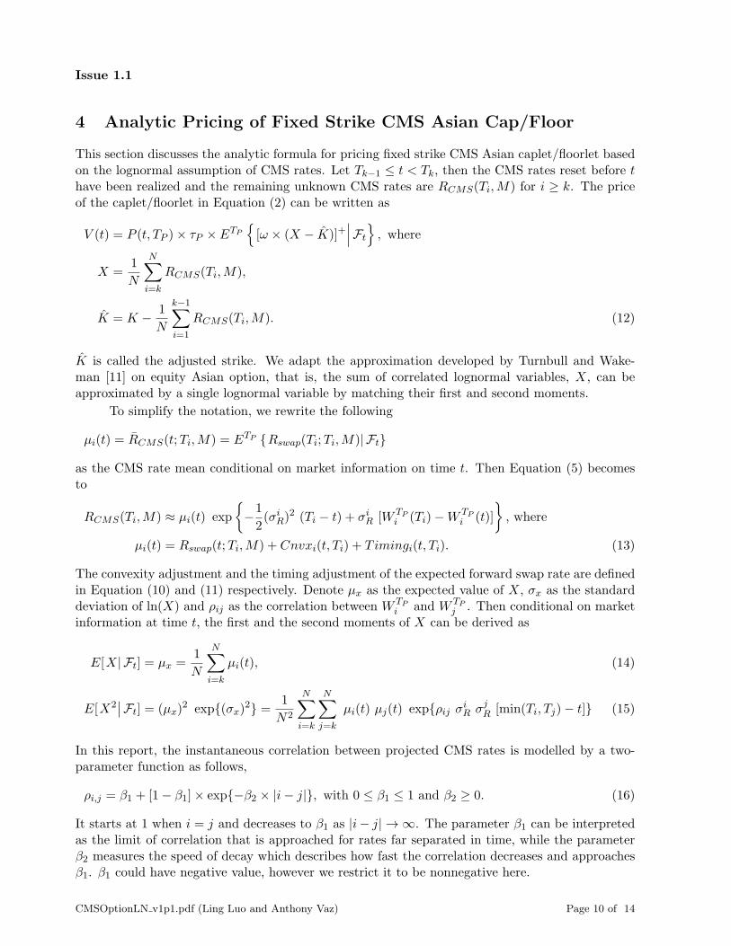
4 Analytic Pricing of Fixed Strike CMS Asian Cap/Floor

This section discusses the analytic formula for pricing fixed strike CMS Asian caplet/floorlet basedon the lognormal assumption of CMS rates. Let Tk−1 ≤ t < Tk, then the CMS rates reset before thave been realized and the remaining unknown CMS rates are RCMS(Ti,M) for i ≥ k. The priceof the caplet/floorlet in Equation (2) can be written as

V (t) = P (t, TP )× τP × ETP

{[ω × (X − K̂)]+

∣∣∣Ft

}, where

X =1

N

N∑i=k

RCMS(Ti,M),

K̂ = K − 1

N

k−1∑i=1

RCMS(Ti,M). (12)

K̂ is called the adjusted strike. We adapt the approximation developed by Turnbull and Wake-man [11] on equity Asian option, that is, the sum of correlated lognormal variables, X, can beapproximated by a single lognormal variable by matching their first and second moments.

To simplify the notation, we rewrite the following

µi(t) = R̄CMS(t;Ti,M) = ETP {Rswap(Ti;Ti,M)| Ft}

as the CMS rate mean conditional on market information on time t. Then Equation (5) becomesto

RCMS(Ti,M) ≈ µi(t) exp

{−1

2(σi

R)2 (Ti − t) + σi

R [W TPi (Ti)−W TP

i (t)]

}, where

µi(t) = Rswap(t;Ti,M) + Cnvxi(t, Ti) + Timingi(t, Ti). (13)

The convexity adjustment and the timing adjustment of the expected forward swap rate are definedin Equation (10) and (11) respectively. Denote µx as the expected value of X, σx as the standarddeviation of ln(X) and ρij as the correlation between W TP

i and W TPj . Then conditional on market

information at time t, the first and the second moments of X can be derived as

E[X| Ft] = µx =1

N

N∑i=k

µi(t), (14)

E[X2∣∣Ft] = (µx)

2 exp{(σx)2} =1

N2

N∑i=k

N∑j=k

µi(t) µj(t) exp{ρij σiR σj

R [min(Ti, Tj)− t]} (15)

In this report, the instantaneous correlation between projected CMS rates is modelled by a two-parameter function as follows,

ρi,j = β1 + [1− β1]× exp{−β2 × |i− j|}, with 0 ≤ β1 ≤ 1 and β2 ≥ 0. (16)

It starts at 1 when i = j and decreases to β1 as |i− j| → ∞. The parameter β1 can be interpretedas the limit of correlation that is approached for rates far separated in time, while the parameterβ2 measures the speed of decay which describes how fast the correlation decreases and approachesβ1. β1 could have negative value, however we restrict it to be nonnegative here.


Issue 1.1

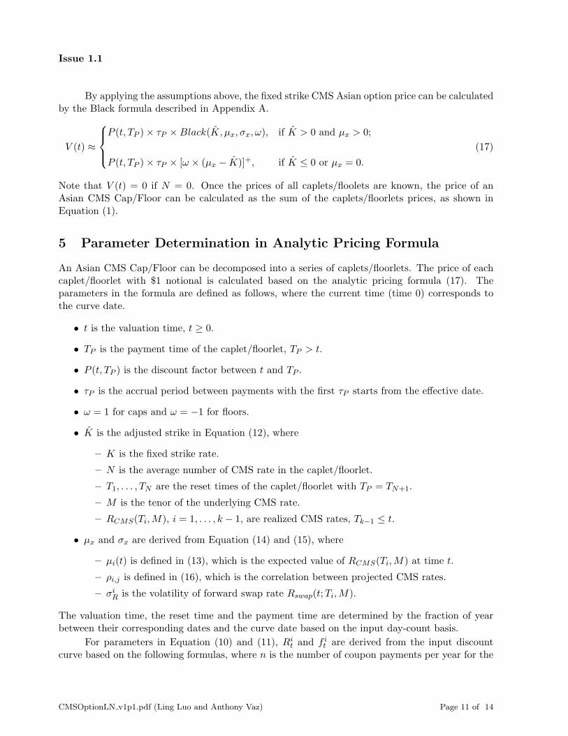
By applying the assumptions above, the fixed strike CMS Asian option price can be calculatedby the Black formula described in Appendix A.

V (t) ≈

P (t, TP )× τP ×Black(K̂, µx, σx, ω), if K̂ > 0 and µx > 0;

P (t, TP )× τP × [ω × (µx − K̂)]+, if K̂ ≤ 0 or µx = 0.

(17)

Note that V (t) = 0 if N = 0. Once the prices of all caplets/floolets are known, the price of anAsian CMS Cap/Floor can be calculated as the sum of the caplets/floorlets prices, as shown inEquation (1).

5 Parameter Determination in Analytic Pricing Formula

An Asian CMS Cap/Floor can be decomposed into a series of caplets/floorlets. The price of eachcaplet/floorlet with $1 notional is calculated based on the analytic pricing formula (17). Theparameters in the formula are defined as follows, where the current time (time 0) corresponds tothe curve date.

• t is the valuation time, t ≥ 0.

• TP is the payment time of the caplet/floorlet, TP > t.

• P (t, TP ) is the discount factor between t and TP .

• τP is the accrual period between payments with the first τP starts from the effective date.

• ω = 1 for caps and ω = −1 for floors.

• K̂ is the adjusted strike in Equation (12), where

– K is the fixed strike rate.

– N is the average number of CMS rate in the caplet/floorlet.

– T1, . . . , TN are the reset times of the caplet/floorlet with TP = TN+1.

– M is the tenor of the underlying CMS rate.

– RCMS(Ti,M), i = 1, . . . , k − 1, are realized CMS rates, Tk−1 ≤ t.

• µx and σx are derived from Equation (14) and (15), where

– µi(t) is defined in (13), which is the expected value of RCMS(Ti,M) at time t.

– ρi,j is defined in (16), which is the correlation between projected CMS rates.

– σiR is the volatility of forward swap rate Rswap(t;Ti,M).

The valuation time, the reset time and the payment time are determined by the fraction of yearbetween their corresponding dates and the curve date based on the input day-count basis.

For parameters in Equation (10) and (11), Rit and f i

t are derived from the input discountcurve based on the following formulas, where n is the number of coupon payments per year for the


Issue 1.1

fixed leg of the swap.

Ri0 = Rswap(0;Ti,M) = n× P (0, Ti)− P (0, Ti +M)∑nM

k=1 P (0, Ti + k/n)

f i0 = ffwd(0;Ti, TP ) = n×

[(P (0, TP )

P (0, Ti)

)−1/[n(Tp−Ti)]

− 1

], TP > Ti

Here Ti is the reset time for Rswap(0;Ti,M). Discount factors are log-linearly interpolated from theinput discount curve with flat extension of continuous compounded zero rates at both ends of thecurve. The volatilities σi

R and σif are linearly interpolated from the corresponding input volatility

curve with flat extension of volatilities at both ends of the curve. The correlations ρiR,f are linearlyinterpolated from the input correlation curve with flat extension of volatilities at both ends of thecurve.


Issue 1.1

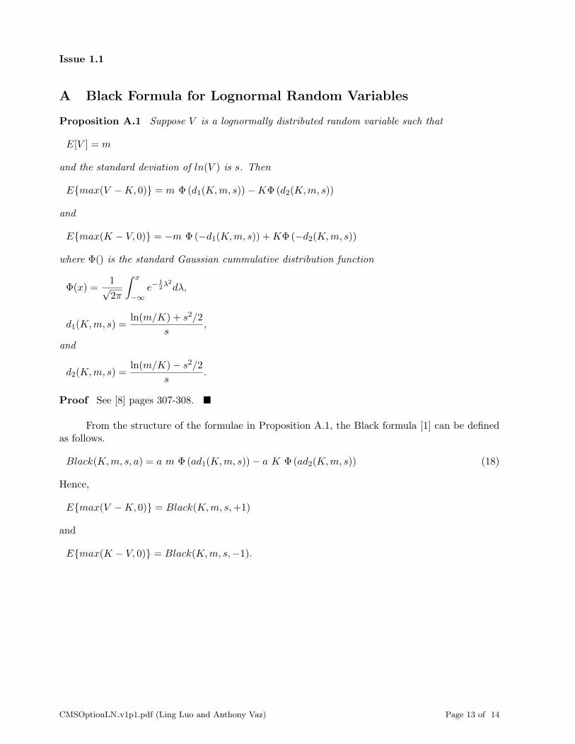
A Black Formula for Lognormal Random Variables

Proposition A.1 Suppose V is a lognormally distributed random variable such that

E[V ] = m

and the standard deviation of ln(V ) is s. Then

E{max(V −K, 0)} = m Φ(d1(K,m, s))−KΦ(d2(K,m, s))

and

E{max(K − V, 0)} = −m Φ(−d1(K,m, s)) +KΦ(−d2(K,m, s))

where Φ() is the standard Gaussian cummulative distribution function

Φ(x) =1√2π

∫ x

−∞e−

12λ2dλ,

d1(K,m, s) =ln(m/K) + s2/2

s,

and

d2(K,m, s) =ln(m/K)− s2/2

s.

Proof See [8] pages 307-308. �

From the structure of the formulae in Proposition A.1, the Black formula [1] can be definedas follows.

Black(K,m, s, a) = a m Φ(ad1(K,m, s))− a K Φ(ad2(K,m, s)) (18)

Hence,

E{max(V −K, 0)} = Black(K,m, s,+1)

and

E{max(K − V, 0)} = Black(K,m, s,−1).


Issue 1.1

References

[1] Damiano Brigo and Fabio Mercurio, Interest Rate Models - Theory and Practice, SpringerVerlag, New York, 2001.

[2] H. Geman, N. El Karoui and J. C. Rochet, “Change of Numeraire, Changes of ProbabilityMeasures and Pricing of Options”, Journal of Applied Probability, Vol. 32, 443-458, 1995.

[3] Patrick Hagan, “Convexity conundrums: Pricing CMS Swaps, Caps and Floors”, WilmottMagazine, March 2003, p.38-44.

[4] Michael Harrison and Stanley Pliska, “Martingales and Stochastic integrals in the theory ofcontinuous trading”, Stochastic Processes and their Applications, Volume 11, No.3, pp. 215260,1981.

[5] Espen Gaarder Haug, The Complete Guide to Option Pricing Formulas, 2nd edition, McGraw-Hill, New York, 2006.

[6] Vicky Henderson and Rafal Wojakowski, “On the Equivalence of Floating and Fixed StrikeAsian Options”, Journal of Finance, Vol. 52, No. 3, pp.923-973, 2001.

[7] Vicky Henderson, David Hobson, William Shaw, and Rafal Wojakowski, “Bounds for in-progress floating-strike Asian options using symmetry”, Annals of Operations Research, Vol.151, No. 1, pp. 81 - 98, 2007.

[8] John Hull, Options, Futures, and Other Derivative Securities, 7th edition, Prentice Hall, NewJersey, 2009.

[9] F. A. Longstaff and E. S. Schwartz, “Valuing American Options by Simulation: A SimpleLeast-Squares Approach”, Review of Financial Studies, Vol. 14, No. 1, pp. 113147, 2001.

[10] Marek Musiela and Marek Rutkowski, Martingale Methods in Financial Modelling, SpringerVerlag, New York, 1997.

[11] Stuart Turnbull and Lee Wakeman, “A Quick Algorithm for Pricing European Average Op-tions”, Journal of Financial and Quantitative Analysis, Vol. 26, No. 3, September 1981, pp.377-389.


Documents

Fixed Strike Asian Cap/Floor on CMS Rates with Lognormal ...€¦ · Fixed Strike Asian Cap/Floor on CMS Rates with Lognormal Approach July 27, 2011 Issue 1.1 Prepared by ... We adapt