Embed Size (px)
Citation preview
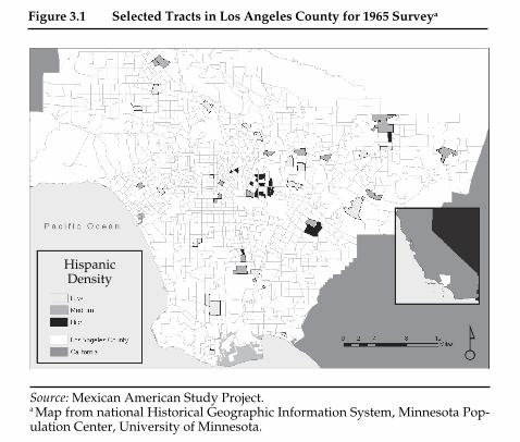
pattern, with the two inner southern rings being high density MexicanAmerican and largely poor, except for the two extreme eastern tracts, whichare poor but mostly African American. The next two rings out from theinner city were traditionally white ethnic working class (especially Germansand Czechs) in the 1960s with upwardly mobile Mexican Americans begin-ning to move in. San Antonio’s deep pattern of segregation precluded theselection of Northside census tracts. By now, the entire Southside is pre-dominately Mexican American and the Northwest is also largely populatedby Mexican Americans as well as the white working and middle class.12
For readers familiar with either area, these maps confirm that respondentscame from a wide diversity of neighborhoods.
The 2000 Mexican American Study Project
In addition to reanalyzing the 1965 data, we also decided to pursue a farmore ambitious goal. We would try to find and interview the survivingoriginal respondents, as well as their children. Based on a pilot test offinding a sample of Los Angeles residents, we came to discover that the
52 Generations of Exclusion
Source: Mexican American Study Project.a Map from national Historical Geographic Information System, Minnesota Pop-ulation Center, University of Minnesota.
HispanicDensity
Figure 3.1 Selected Tracts in Los Angeles County for 1965 Surveya
task would require much detective-like work, making it even harder thananticipated. This would be a multiyear project and would require sub-stantial funding. By mid-1994, we had secured enough to hire severalgraduate students and begin searching for the original respondents. In1997, a large grant enabled us to conduct the actual interviews. Indeed,the process of finding and interviewing respondents would take severalyears and involved several arduous tasks, which we will describe.
We set out to reinterview the original respondents who were ageeighteen to fifty in 1965 and 1966 and in their early fifties to early eightiesduring the 1998 to 2000 follow-up. We omitted the 24 percent who wereover fifty in 1965 and 1966 because of the high probability that they wouldhave died by 1998. When the original respondents age fifty and younger haddied, we searched for family members and conducted an interview aboutthe respondent, which we refer to as informant interviews. In addition,we sought to interview the children of respondents who were younger thaneighteen in 1965 and therefore in their early thirties to early fifties in 1998.The selection method for the original respondents was therefore straight-forward. The sample had been drawn in the 1960s. Our plan was to simply
The Mexican American Study Project 53
Figure 3.2 Selected Tracts in San Antonio (Bexar County) for 1965 Surveya
Source: Mexican American Study Project.a Map from national Historical Geographic Information System, Minnesota Pop-ulation Center, University of Minnesota.
HispanicDensity
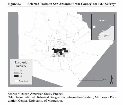
Family generation appears on the horizontal axis in figure 3.1 andindicates historical change. We also break the sample into generations-since-immigration, which is denoted on the vertical axis of figure 3.1.Generation-since-immigration refers to the number of generations sincethe immigrants arrived in the United States. Figure 3.3 summarizes therelation between the family generation and generation-since-immigrationin our study. It shows, for example, that third-generation children hadimmigrant grandparents and that the fourth-generation children hadgreat-grandparents who immigrated at a still earlier period.
The bold octagon defines the two family generations and four generations-since-immigration used in our study. That is, we capture amore dynamic process of real generational change, as required for testinghypotheses of assimilation or ethnic change. This compares to the stan-dard intergenerational comparisons based on cross-sectional data, whichis denoted by the dashed lines on figure 3.3. Such designs are based on
68 Generations of Exclusion
Family Generation
1
2
3
4
Generation-Since-Immigration
OurIntergenerational Design
TypicalCross-Sectional Design
Great-Grandparents Grandparents
Parents (OriginalRespondents) Children
(Immigrants)
Source: Authorsí compilation.
Figure 3.3 Two Dimensions of Generational Change
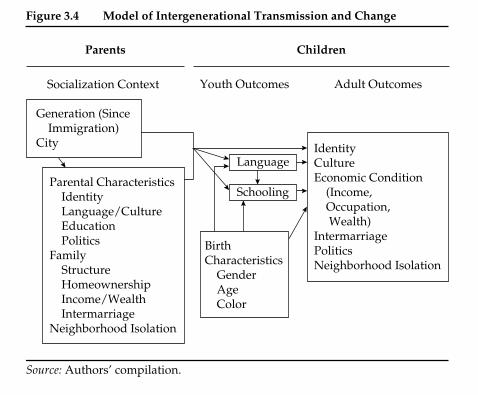
Our Multivariate Model
Aside from examining the extent of change from original respondents totheir children, we are also interested in understanding the factors mostassociated with that change. For example, if children are more likely toattend college than their parents, is it generation that led to the changeor some other factor? Could greater college attendance be due to greaterresources that later generation parents have accrued and that perhapspermitted them to provide for a better education for their children, eitherbecause they moved out of the barrio or because they paid for private edu-cation? Similarly, how are changes in ethnic identity or Spanish-languageproficiency associated with such factors?
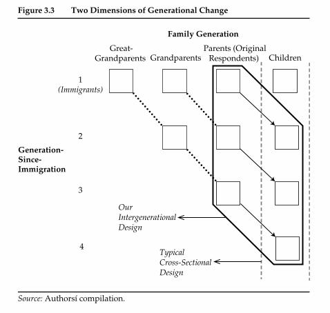
We present our basic model of intergenerational transmission andchange in figure 3.4. The model reads from left to right, beginning with theexogenous characteristics of generation and urban area (Los Angeles Countyor San Antonio City). We are interested, above all, on how generation-since-immigration and, to a lesser extent, urban area are related to theoutcomes for both the original respondents and their children. An analysisof these variables seeks to answer the question like, “to what extent does
70 Generations of Exclusion
Source: Authors’ compilation.
Parents Children
Youth Outcomes Adult OutcomesSocialization Context
Language
Schooling
BirthCharacteristics
GenderAgeColor
Parental CharacteristicsIdentityLanguage/CultureEducationPolitics
FamilyStructureHomeownershipIncome/WealthIntermarriage
Neighborhood Isolation
IdentityCultureEconomic Condition
(Income, Occupation, Wealth)
IntermarriagePoliticsNeighborhood Isolation
Generation (Since Immigration)
City
Figure 3.4 Model of Intergenerational Transmission and Change
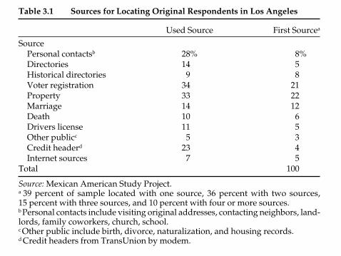
Table 3.1 Sources for Locating Original Respondents in Los Angeles
Used Source First Sourcea
SourcePersonal contactsb 28% 8%Directories 14 5Historical directories 9 8Voter registration 34 21Property 33 22Marriage 14 12Death 10 6Drivers license 11 5Other publicc 5 3Credit headerd 23 4Internet sources 7 5
Total 100
Source: Mexican American Study Project.a 39 percent of sample located with one source, 36 percent with two sources, 15 percent with three sources, and 10 percent with four or more sources.b Personal contacts include visiting original addresses, contacting neighbors, land-lords, family coworkers, church, school.c Other public include birth, divorce, naturalization, and housing records.d Credit headers from TransUnion by modem.
cial sources but do not include any of the financial data. With special per-mission granted to us as researchers, we also accessed CaliforniaDepartment of Motor Vehicles records. Having access to these sources ofinformation shifted most of the searching activities from field work to ourproject offices.
The final stage of our search process coincided with the availability ofinformation through the Internet, including much information we hadpreviously secured in CD format. The availability had many benefits.First, it was easier to identify and purchase sources of information oncompact disks, such as California Property, Texas People Finder, andTexas Property. Second, national phone directories became available.Third, the Internet permitted more powerful and flexible searchingstrategies. Last, Internet data sets merged large quantities of data frommultiple sources.
In sum, technological developments improved our ability to find respon-dents over the course of our search. Additionally, we had devised manycreative ways of searching when we had exhausted the normal search pro-cedures. Table 3.1 presents the sources we used to locate respondents,grouped into broad categories. The first column presents the percentage ofcases that we used, by type of source, in the search process. Because multi-ple sources could be used to locate a respondent, the percentages in the first
56 Generations of Exclusion
homeownership, marriage, children, household composition, and income.The survey ended up being forty-five to seventy-five minutes long, largelydepending on how many questions applied to the respondent. We designedseparate questionnaires each for original respondents, children of respon-dents, and informants for the original respondents. The original respondentand informant questionnaires were made available in English and Spanish.17
For original respondents who had died, we interviewed an informant,which was usually the surviving spouse but sometimes an adult child orother close family member. The informant questionnaire was much like thatfor the respondent, but without attitudinal questions and those for whichwe believed informants could not provide reliable answers. It includedquestions on place of birth, language use, contact with other groups, edu-cational level, employment status, marital status, household composition,income, and children.
The Los Angeles interviews were conducted by the Survey ResearchCenter (SRC) of UCLA’s Institute for Social Science Research (ISSR), andthe San Antonio sample by a Texas-based firm, NuStats Research andConsulting in Austin. Interviews were primarily conducted in respondents’homes. Contact information was forwarded from the UCLA project staff toSRC and NuStats field staff to facilitate appointment setting for interview-ing. Contact was first made with the original respondent and after thatwith randomly selected children of the respondent. Respondents werepaid an incentive of $20 for their participation.
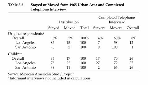
In some cases, we were unable to interview respondents face to face,usually for those who moved out of metropolitan Los Angeles or SanAntonio. The first three columns of table 3.2 show the proportion of respon-
58 Generations of Exclusion
Table 3.2 Stayed or Moved from 1965 Urban Area and CompletedTelephone Interview
Completed Telephone Distribution Interview
Stayed Moved Total Stayers Movers Overall
Original respondentsa
Overall 93% 7% 100% 4% 60% 8%Los Angeles 85 15 100 7 58 12San Antonio 98 2 100 0 100 1
ChildrenOverall 83 17 100 17 70 26
Los Angeles 78 22 100 27 72 37San Antonio 89 11 100 2 66 26
Source: Mexican American Study Project.a Informant interviews not included in calculations.

dents who had moved and the final three show the percentage of movers,stayers, and the overall sample who were interviewed by phone. Anywherefrom 2 to 22 percent of respondents moved out of the two metropolitanareas by 2000. Most of those who moved, but only a few of those whostayed, were interviewed by telephone. For three of the four cases, nomore than 7 percent of the stayers were interviewed by phone. The excep-tion was the 27 percent of children in Los Angeles, most of whom livedoutside of Los Angeles County but within the five-county metropolitanarea. Although we consider them stayers, many were often at a consider-able distance, making personal interviews difficult.18
Success in Locating and InterviewingOriginal Respondents
We located nearly four of every five (79 percent) of the original respondents,as shown in table 3.3. We did have a higher number of refusals thanexpected, however, and were able to interview only 73 percent of those wefound. In the end, we interviewed nearly three of every five (57 percent)of the original respondents who were age fifty or less in 1965.
Most of our nonresponses were refusals. For the most part, we found thatrespondents were receptive and often surprised when we located them.Most did not remember being interviewed more than thirty years earlier.Many, however, were curious that we had located them after so manyyears, especially when they did not recall participating in the original study.Some were suspicious or concerned that we were able to do so and thussometimes refused to be interviewed. Additionally, by 2000, many of ouroriginal respondents had become elderly. We were up against a publicservice campaign at the time aimed at Latino elderly, which warned themto be careful of solicitors, telemarketers, or any stranger coming to thedoor or calling.
The Mexican American Study Project 59
Table 3.3 Searched, Located, and Interviewed Original Respondents by Urban Area
Total Los Angeles San Antonio
a. Searched 1,193 792 401b. Located 941 614 327c. Interviewed 684 434 250
Located of total (b/a) 79% 78% 82%Interviewed of located (c/b) 73 71 76Response rate (c/a) 57 55 62
Source: Mexican American Study Project.
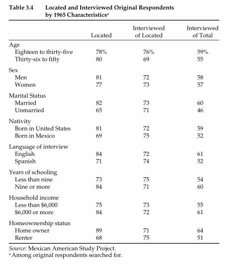
out of the total sample searched for is listed in column 1; the percent ofpersons interviewed among those whom we found are listed in column 2;the final percent interviewed out of the total sample is shown in column 3.For example, the first row shows that persons age eighteen to thirty-five in1965 were slightly less likely to be located than those older than thirty-five,but, when they were located, were more likely to be interviewed. Even-tually, we ended up interviewing 59 percent of the younger respondentsto the original survey and 55 percent of the older respondents. Men wereslightly more likely to be interviewed than women. The differences, though,were greater for all of the other variables. Married persons, those born in
The Mexican American Study Project 61
Table 3.4 Located and Interviewed Original Respondents by 1965 Characteristicsa
Interviewed Interviewed Located of Located of Total
AgeEighteen to thirty-five 78% 76% 59%Thirty-six to fifty 80 69 55
SexMen 81 72 58Women 77 73 57
Marital StatusMarried 82 73 60Unmarried 65 71 46
NativityBorn in United States 81 72 59Born in Mexico 69 75 52
Language of interviewEnglish 84 72 61Spanish 71 74 52
Years of schoolingLess than nine 73 75 54Nine or more 84 71 60
Household incomeLess than $6,000 75 73 55$6,000 or more 84 72 61
Homeownership statusHome owner 89 71 64Renter 68 75 51
Source: Mexican American Study Project.a Among original respondents searched for.
the United States, those interviewed in English, the more educated, thewealthier, and homeowners were all more likely to be interviewed thantheir counterparts.20
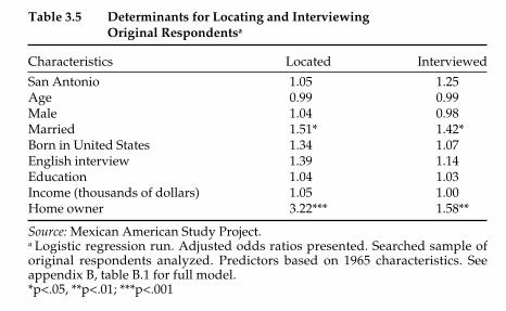
Because many of these variables are interrelated, effects are not neces-sarily independent. For example, persons born in the United States aremore likely to have answered the interview in English, received moreschooling, and owned their homes. It may therefore be that birthplacedrives the differences on language, education, and homeownership. It mayalso be, however, that one or more of these variables have an additionalindependent effect. To determine which variables are responsible or instatistical parlance, which have an independent and significant effect, weran a statistical analysis to predict locating and interviewing respondents.Specifically, we used logistic regression analysis to regress a binary vari-able indicating whether we found a respondent and secured an interviewin the follow-up on a set of potential explanatory variables drawn fromthe 1965 data. The results are shown on table 3.5 (where we present oddratios). Column 1 shows that only two variables were statistically signifi-cant in locating the original respondents: married persons were 1.5 timesmore likely to be found than unmarried, and homeowners were fully 3.2 times more likely than renters, net of all other effects. The other vari-ables, including city of residence, were not independently influential fac-tors and are apparently correlated with homeownership and perhaps alsowith married status. In other words, the fact that we found more SanAntonio respondents seems largely because they are more likely to behomeowners than respondents in Los Angeles.
62 Generations of Exclusion
Table 3.5 Determinants for Locating and Interviewing Original Respondentsa
Characteristics Located Interviewed
San Antonio 1.05 1.25Age 0.99 0.99Male 1.04 0.98Married 1.51* 1.42*Born in United States 1.34 1.07English interview 1.39 1.14Education 1.04 1.03Income (thousands of dollars) 1.05 1.00Home owner 3.22*** 1.58**
Source: Mexican American Study Project.a Logistic regression run. Adjusted odds ratios presented. Searched sample oforiginal respondents analyzed. Predictors based on 1965 characteristics. Seeappendix B, table B.1 for full model.*p<.05, **p<.01; ***p<.001

Those weights are shown in the matrix on table 3.6. Based on the originalrespondent’s homeownership, marital status, city of residence, and incomeduring the original survey, the values in table 3.6 show the extent to whichtheir representation was weighted in the follow-up sample. At one end,married and low-income homeowners who lived in Los Angeles wereespecially likely to have been reinterviewed and thus were given the low-est weight (.584). At the other extreme, unmarried and low income rentersin San Antonio were least likely to be found in the follow-up survey andthus were given the greatest weight. The representation of such personswas inflated more than two times (2.103). With the exception of these twocategories, the other fourteen categories of original respondents fell withina fairly narrow range (.779 to 1.244), which suggests that selectivity wasnot especially problematic.
The 2000 Children Sample
For the child sample, who were adults in 2000, we selected a randomsample of the original respondents’ children born between 1947 and 1966.We selected a maximum of two children for each original respondent.22
When original respondents had one or two children who met the selectioncriteria, all were selected. When more than two children met the criteria,we chose the most recent birthdate.23 As can be seen in table 3.7, ninety-twofamilies had no children who met the criteria, 100 had one, 146 had two,and 358 had three or more. In summary, 2,004 children met the age criteria,1,108 were selected, and 758 (68 percent of those selected) were interviewed.
We selected and located children based on information from the parentswe interviewed. First, we completed a roster of all the original respondents’children, with information on sex, name, birth month and year, biologicalrelationship, country of birth, status (employed, in the military, laid off orunemployed, keeping house, in school, in prison or institution, deceased),
64 Generations of Exclusion
Table 3.6 Weights for Bivariate Analyses with Original Respondentsa
Poor Not Poor
Married Unmarried Married Unmarried
Los AngelesHomeowner 0.584 0.779 0.949 1.168Not homeowner 1.103 1.256 1.126 1.244
San AntonioHomeowner 0.861 1.635 0.809 0.949Not homeowner 1.038 2.103 0.883 1.071
Source: Mexican American Study Project.a Based on 1965 characteristics.

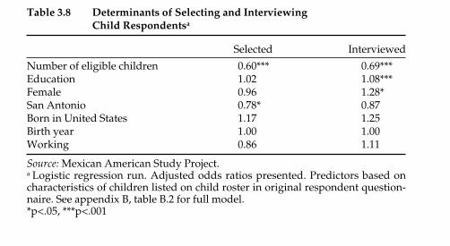
years of education, and whether living with the original respondent parentin 1965 and 1966. We used this information to select children and to deter-mine whether the characteristics of children we interviewed biased thesample in any way. We then determined bias by regressing a binary vari-able for whether we selected a respondent or secured an interview on aset of potential explanatory variables drawn from the child roster.
The results are shown on table 3.8, where we present odd ratios.Column 1 shows the results for selecting the child respondents and col-umn 2 shows the results for interviewing children out of all eligible chil-dren. The number of children in the family had a strong relationship toboth selecting and interviewing children, which was a direct result of ourselection strategy. In families with one or two eligible children, each childhad a 100 percent chance of being selected, whereas in families with three
The Mexican American Study Project 65
Table 3.7 Eligible, Selected, and Interviewed Child Respondentsa
Three to No One Two Twelve
Eligible Eligible Eligible EligibleTotal Children Child Children Children
a. Families 696 92 100 146 358b. Eligible children 2,004 0 100 292 1,612c. Selected children 1,108 0 100 292 716d. Interviewed children 758 0 65 207 486
Response rate (d/c) 68% — 65% 71% 69%
Source: Mexican American Study Project.a Among children listed on roster in original respondent questionnaire.
Table 3.8 Determinants of Selecting and Interviewing Child Respondentsa
Selected Interviewed
Number of eligible children 0.60*** 0.69***Education 1.02 1.08***Female 0.96 1.28*San Antonio 0.78* 0.87Born in United States 1.17 1.25Birth year 1.00 1.00Working 0.86 1.11
Source: Mexican American Study Project.a Logistic regression run. Adjusted odds ratios presented. Predictors based oncharacteristics of children listed on child roster in original respondent question-naire. See appendix B, table B.2 for full model.*p<.05, ***p<.001
These theories, however, often treat generation-since-immigration as coter-minous with family generation, for example, from grandparents, who areoften but not always immigrant, to child to grandchild. A significant over-lap between family generation and generation-since-immigration mayhave been the experience of many European ethnics but it implies sometheoretical and methodological confusion. Empirically, it is very trouble-some in understanding the Mexican American case.
Parsing family generation from generation-since-immigration is par-ticularly important, and complex, for Mexicans, whose history of immi-gration has been, for the most part, throughout the twentieth century. Forexample, the relatively small population born in the United States before1910 intermarried extensively with the larger population of 1910 to 1930immigrants, and their U.S.-born children have intermarried with theimmigrants from subsequent waves. This generational complexity hasbeen a significant issue in studies even though assimilation theories rarelydeal with it. That they do not is not surprising, given the immigrationexperience of most groups.
The classic road to assimilation involved immigration in a relativelycompressed time and thus generational change was generally uniform forentire ethnic groups. Massive immigration from Central and SouthernEurope occurred during a short period in the late nineteenth and earlytwentieth centuries, so that the subsequent history of the group coincidedlargely with the experience of single generations-since-immigration. Italianimmigration, the bulk of which occurred from 1900 to 1914, is a goodexample.25 We seek to resolve this problem, which we illustrate in figure 3.3.
The Mexican American Study Project 67
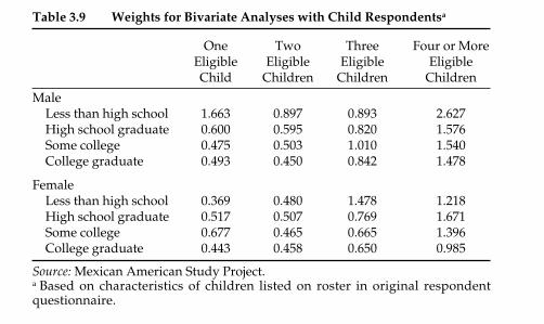
Table 3.9 Weights for Bivariate Analyses with Child Respondentsa
One Two Three Four or More Eligible Eligible Eligible Eligible Child Children Children Children
MaleLess than high school 1.663 0.897 0.893 2.627High school graduate 0.600 0.595 0.820 1.576Some college 0.475 0.503 1.010 1.540College graduate 0.493 0.450 0.842 1.478
FemaleLess than high school 0.369 0.480 1.478 1.218High school graduate 0.517 0.507 0.769 1.671Some college 0.677 0.465 0.665 1.396College graduate 0.443 0.458 0.650 0.985
Source: Mexican American Study Project.a Based on characteristics of children listed on roster in original respondentquestionnaire.
interviews bias the responses. Second, it serves as a proxy measure forpersons who moved out of the area. In particular, we expect that those whodid may be among the more assimilated sectors of the population, andthus it is important to measure or control for this effect. On an indicatorsuch as residential segregation, for example, we would expect personswho were interviewed by telephone to have moved to neighborhoods withfewer other Mexican Americans, because they are likely to have left theethnically dense Los Angeles or San Antonio urban areas.
Generation-Since-Immigration of Childrenas Used in the Multivariate Analyses
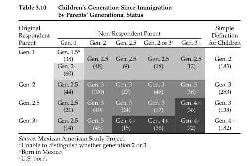
For the multivariate analysis, the children are the primary unit of analysis.This permits us to use parental characteristics for determining child out-comes and to examine generation in greater detail. Whereas a child’s gen-eration in the bivariate analysis is determined as simply the originalrespondent’s generation plus one, for the multivariate analysis we calcu-late the child’s generation based on birthplace and the generation of bothparents. We thus allow for greater generational complexity than in thebivariate analysis by computing half or .5 generations.
Table 3.10 shows the distribution by generation of the 720 U.S.-bornchildren in our sample, according to the generation of both their parents.
72 Generations of Exclusion
Non-Respondent Parent
Table 3.10 Children’s Generation-Since-Immigration by Parents’ Generational Status
Original Simple Respondent Definition Parent Gen. 1 Gen. 2 Gen. 2.5 Gen. 2 or 3a Gen. 3+ for Children
Gen. 1 Gen. 1.5b
(38) Gen. 2.5 Gen. 2.5 Gen. 2.5 Gen. 2.5 Gen. 2 Gen. 2c (48) (9) (18) (12) (185)
(60)
Gen. 2 Gen. 2.5 Gen. 3 Gen. 3 Gen. 3 Gen. 3 Gen. 3 (44) (100) (27) (46) (36) (253)
Gen. 2.5 Gen. 2.5 Gen. 3 Gen. 3 Gen. 3 Gen. 4+ Gen. 3 (21) (40) (24) (17) (36) (138)
Gen. 3+ Gen. 2.5 Gen. 3 Gen. 4+ Gen. 4+ Gen. 4+ Gen. 4+(14) (45) (15) (36) (72) (182)
Source: Mexican American Study Project.a Unable to distinguish whether generation 2 or 3.b Born in Mexico.c U.S. born.
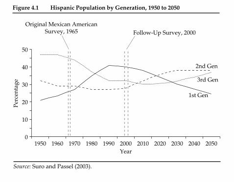
Rodolfo Alvarez,81 the Mexican American generation had arrived to succeeda Mexican immigrant generation and that demographic shift would produce new assimilationist hopes.82 The historian Vicki Ruíz, however,contended that such generational distinctions were often ambiguous inpractice.83 Figure 4.1 shows the changing generational composition of the Hispanic population from 1950 to 2050. By the 1950s, nearly half ofHispanics were third generation or more, given that mass immigration fromLatin America had ended before 1930. The third generation, however, beganto shrink in the 1960s as large-scale Mexican immigration reemerged.
The image of Mexicans and Mexican Americans continued to be poor.The animosity toward Mexicans was apparent in a sensationalist press thatreinforced anti-Mexican stereotypes,84 depicting Mexican American youthas “the enemy within.” It became especially heated with the Zoot Suit Riots in 1943, when white sailors systematically and repeatedly attackedMexican American youth.85 Negative stereotypes of Mexicans wouldpersist and occasionally enter the public discourse as in Judge GeraldChargin’s 1969 tirade against a juvenile who had pled guilty to incest:
Mexican people, after 13 years of age, it’s perfectly all right to go out andact like an animal . . . You are lower than animals and haven’t the right tolive in organized society—just miserable, lousy, rotten people.86
86 Generations of Exclusion
Original Mexican AmericanSurvey, 1965 Follow-Up Survey, 2000
01950 1960 1970 1980 2000 20201990 2010 2030 2040 2050
10
20
30
40
50
Perc
enta
ge
Year
Source: Suro and Passel (2003).
1st Gen
3rd Gen
2nd Gen
Figure 4.1 Hispanic Population by Generation, 1950 to 2050
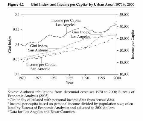
inequality increased in both Los Angeles and San Antonio since 1970, justas it did throughout the United States. The growing inequality mirroredthe structural transformations from heavy manufacturing and highlypaid and unionized blue-collar jobs and toward a service and light man-ufacturing economy characterized by both a growing number of highpaying white-collar work and low paying manual jobs with little job secu-rity. Although inequality in the two urban areas was similar from 1970 to1980, it grew more in San Antonio in the 1980s. However, by the 1990s,inequality shot up in Los Angeles but remained nearly flat in San Antonio,eventually resulting in greater income inequality in Los Angeles.
Nationally, industrial jobs declined numerically from the 1970s for-ward as the United States faced growing competition from foreign indus-tries; concomitantly, the service sector grew. As a result, average incomesdeclined as the number of middle-income blue-collar jobs dropped, lead-ing to a growing hourglass shape to the economy. Blue-collar jobs at the time had afforded relatively high pay and internal career mobilityfor the largely unionized workforce. The new jobs in the low-wageindustries tended to be low paying, low skilled, relatively unstable, and
98 Generations of Exclusion
Source: Authorsí tabulations from decennial censuses 1970 to 2000; Bureau of Economic Analysis (2005).a Gini index calculated with personal income data from census data.b Income per capita based on personal income divided by population size; calcu-lated by Bureau of Economic Analysis; and adjusted to 2000 dollars. c Data for Los Angeles and Bexar Counties.
0.3
0.35
0.4
0.45
0.5
1970 1975 1980 1985Year
1990 1995 2000
Gin
i Ind
ex
10,000
15,000
20,000
25,000
30,000
35,000
Inco
me
per
Cap
ita
Income per Capita,Los Angeles
Income per Capita,San Antonio
Gini Index,San Antonio
Gini Index,Los Angeles
Figure 4.2 Gini Indexa and Income per Capitab by Urban Areac, 1970 to 2000

80 Generations of Exclusion
labor migration across the border also seemed at the time a more com-mon pattern than permanent immigration.40 Mexico’s modernizationproject, led by President Porfirio Díaz from 1880 to 1910, would displacemillions of peasants from their lands as they left to work primarily in therapidly developing mines and railroad construction within Mexico butthat resulted mostly in internal migration. However, by 1907, the bottomhad fallen out of the Mexican economy and the Porfirian administrationbecame increasingly unstable. In response, a decade-long Mexican Revo-lution had begun by 1910.41
Also by 1910, the railroads had greatly expanded their Southwestroutes and linked them to Mexico’s new rail system, which would allowMexicans deep in the interior to migrate to the United States. The MexicanRevolution and the growing need for cheap labor in American Southwest,especially in California’s exploding agricultural sector but also in Texasagriculture and cattle-production, would provoke the immigration oflarge numbers of Mexicans.42 Moreover, by 1909, labor recruiting agentshad become active in El Paso and other border cities. These agents wouldsolicit and direct the often temporary migrants to distant American cities
Table 4.1 Mexican Origin Population in, and Legal Mexican Immigrationto, United States, 1850 to 2000
Mexican OriginPopulation Mexican Immigrantsa
Immigrants toYear Population Period Admitted Residents
1850 81,508 — — —1880 290,642 — — —1900 401,491 1901 to 1910 49,642 12.4%1910 640,104 1911 to 1920 219,004 34.21920 999,535 1921 to 1930 459,287 46.01930 1,500,000b 1931 to 1940 22,319 1.51940 1,567,596 1941 to 1950 60,589 3.91950 2,489,477 1951 to 1960 299,811 12.01960 4,087,546 1961 to 1970 453,937 11.11970 5,641,956 1971 to 1980 640,294 11.31980 8,740,439 1981 to 1990 1,655,843 18.91990 13,495,938 1991 to 2000 2,249,421 16.72000 22,338,000 2001 to 2010c 1,790,487 8.0
Source: Gratton and Guttmann (2000); Rumbaut (2006); U.S. Immigration andNaturalization Service (2005); Office of Immigration Statistics (2003).a Immigration statistics not available for Mexicans for 1886 to 1894 and, whenavailable, often did not include land arrivals.b Estimate.c Projection based on immigrant admits in 2001 to 2003 continuing at same rateuntil 2010.
90 Generations of Exclusion
the new laws well into the 1960s and after, often using a series of sub-terfuges to avoid integration.108
The extent of educational segregation before the 1960s is not wellknown. Surveys of particular school districts report that 90 percent of thesedistricts in Texas and 85 percent in California were racially segregated.109
Also, segregation was often limited to elementary school education whilenearly all high schools in San Antonio and Los Angeles were mixed.110
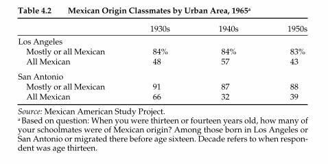
Data from our study permit us to estimate levels of school segregation forthe period in Los Angeles County and San Antonio at roughly the middleschool level. Based on the 1965 data on original respondents collectedby Grebler, Moore, and Guzmán, table 4.2 shows the percent of MexicanAmericans in Los Angeles and San Antonio reporting that they attendedfully segregated or “Mexican schools” when they were thirteen or four-teen years old. To go back as far as we could, we used the entire originalsample and stratified them by age, estimating the decade in which theywere that age. In addition, we restricted the sample to those living in LosAngeles or San Antonio at that age based on those who were born in ormigrated to Los Angeles or San Antonio before age sixteen.
Table 4.2 shows that 83 or 84 percent of Los Angeles and 87 to 91 per-cent of San Antonio school children had mostly or all Mexican-originschoolmates from the 1930s to the 1950s. In the 1930s, fully 66 percent ofyoung adolescent San Antonians were in fully segregated classrooms,versus 48 percent of Los Angelenos of the same age, reflecting the rela-tively rigid segregation of Texas cities and the fact that the proportionMexican was much larger. The extent of segregation in San Antonio subse-quently declines somewhat until the 1940s, and remains flat to at least the1950s. For Los Angeles, complete segregation is erratic, declining in the 1930s, increasing in the 1940s, and dropping again in the 1950s.111 Onthe other hand, 9 percent of San Antonio respondents and 16 percent of LosAngeles respondents reported that a few or none of their classmates were
Table 4.2 Mexican Origin Classmates by Urban Area, 1965a
1930s 1940s 1950s
Los AngelesMostly or all Mexican 84% 84% 83%All Mexican 48 57 43
San AntonioMostly or all Mexican 91 87 88All Mexican 66 32 39
Source: Mexican American Study Project.a Based on question: When you were thirteen or fourteen years old, how many ofyour schoolmates were of Mexican origin? Among those born in Los Angeles orSan Antonio or migrated there before age sixteen. Decade refers to when respon-dent was age thirteen.
96 Generations of Exclusion
time, San Antonio has seen relatively little immigration in the last fiftyyears. In 1970, only 9 percent of Mexican Americans in San Antonio wereimmigrants. By 1990, only 13 percent were. The comparable figures forthe same years in Los Angeles County were 25 and 47 percent.
Changing Los Angeles and San Antonio Economies
In 1965, Los Angeles and San Antonio offered quite distinct opportunitiesfor Mexican Americans though that difference would change by the endof the twentieth century. The industrial and occupational structures of SanAntonio in the 1960s, along with its segregationist and clientelist politics,clearly afforded fewer opportunities to Mexican Americans than the moreeconomically dynamic and modern Los Angeles did. This is apparent inthe data that Grebler, Moore, and Guzmán collected.
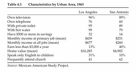
We analyzed data from both waves and present basic economic andsocial indicators in table 4.3. San Antonians were markedly less likely toown televisions and telephones or live in houses with a toilet or hot water.Although roughly 40 percent of San Antonio’s Mexicans earned less than$3,000 annually, only about 13 percent of Angelenos did. Costs of living inthe two cities at the time, interestingly, were similar. Mexican Americanhomes in 1965 already were worth three times as much in Los Angeles.Most notably, though, Angelenos also seemed to be much more accultur-ated on language and religiosity as a much larger percentage of them spokeonly English at home and they less frequently attended religious services.
Largely coinciding with changing patterns of immigration, majorchanges have also occurred in the structure of the United States’ econ-omy since the mid-1970s. With the end of segregation and the most
Table 4.3 Characteristics by Urban Area, 1965
Los Angeles San Antonio
Own television 96% 89%Own telephone 76 60With private toilet 95 89With hot water 99 79Have $500 or more in savings 32 14Monthly income at primary job (mean) $439 $251Monthly income at all jobs (mean) $677 $260Earn less than $3,000 a year 13% 40%Home value (mean) $16,283 $4,902Speak only English to children 31% 10%Frequently attend church 41 62
Source: Mexican American Study Project.

110 Generations of Exclusion
Immigrants, the first generation, age fifty and over
Percent with post-BA diploma
Percent of third and higher-generation
non-Hispanic whites
Percent with nohigh school diploma
Percent with four-yearcollege diploma
AsiaEurope and CanadaSouth AmericaAfro CaribbeanSpanish CaribbeanCentral AmericaPuerto RicoMexico
AsiaEurope and CanadaSouth AmericaAfro CaribbeanSpanish CaribbeanCentral AmericaPuerto RicoMexico
Non-Hispanic whites
Non-Hispanic American Indians
Non-Hispanic AsiansNon-Hispanic blacks
Other Hispanics
Puerto RicoMexico
Native born of native born parents,third and higher generations, age twenty-five to thirty-nine
Native born of foreign or mixed parentage, second generation, age twenty-five to thirty-nine
0
35343117
126121491216
13547111214
8080 6060 4040 2020
Source: Farley and Alba (2002).
Figure 5.1 Educational Attainment by Generation and Origin, 1998 and 2000
Americans (from the West Indian islands and Haiti) do considerably bet-ter. By the third generation, Mexican Americans have the lowest rate at 3 percent, together with African Americans and American Indians.
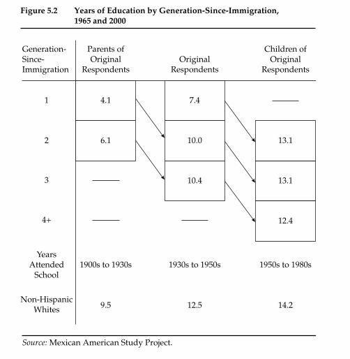
Figure 5.2 shows generational changes for Mexican-origin personsover the span of the twentieth century. In addition to the original respon-dents and their children, we show educational attainment for the parentsof original respondents. The parents were educated mostly in the 1900sto 1930s, the original respondents were schooled from the 1930s to 1950s,and their children were educated from the 1950s to the 1980s. At the sametime, we present results for three generations-since-immigration withineach of these cohorts. Taken together, figure 5.2 shows educational progress
Figure 5.2 Years of Education by Generation-Since-Immigration, 1965 and 2000
Source: Mexican American Study Project.
Generation-Since-Immigration
Parents ofOriginal
Respondents
Children ofOriginal
RespondentsOriginal
Respondents
7.44.1
6.1
1900s to 1930s
9.5 12.5 14.2
1930s to 1950s 1950s to 1980s
1
2
3
4+
YearsAttended
School
Non-HispanicWhites
10.0
10.4
13.1
13.1
12.4
Education 111

Education 113
completed high school, whereas around 80 percent of all children did.18
Understandably, the graduation rate is especially low for immigrantsgiven that they often completed their educations in Mexico, where highschool completion is less common. Only 30 percent of immigrant originalrespondents completed high school, whereas 48 and 57 percent (respec-tively) of their second- and third-generation counterparts did, suggestinga smooth generational improvement for those schooled from the 1930s tothe 1950s. Thus, though improvements from parents to children in grad-uation from high school, especially for immigrants, are clear, they are lessso for the children of the third generation.
Figure 5.3 High School Graduation by Generation-Since-Immigration,1965 and 2000
Source: Mexican American Study Project.a As reported by children, among grandchildren age twenty and older.
Generation-Since-Immigration
OriginalRespondents
Grandchildrenof Original
Respondentsa
Childrenof Original
Respondents
84%
30%
48%
57%
1980s to 1990s1930s to 1950s 1950s to 1980s
1
2
3
4
5+
YearsAttended
School
87%
73%
85%
84%
81%

College Graduate–Gen 2 Original Respondents to Gen 3 Children
High-school Graduate–Gen 2 Original Respondents to Gen 3 Children
High-school Graduate–Gen 3 Original Respondents to Gen 3 Children
College Graduate–Gen 3 Original Respondents to Gen 3 Children
Source: Mexican American Study Project.
Original Respondents (1965) Children (2000)0.1
0.2
0.3
0.4
0.5
0.6
0.7
0.8
Rel
ativ
e od
ds
rati
os
Figure 5.4 Relative Odds Ratios of Mexican Americans to Non-HispanicWhites, 1965 and 2000
inequality because they are not affected, as other indicators of inequality are,by the size of the gap or the specific point at which the gap is measured.
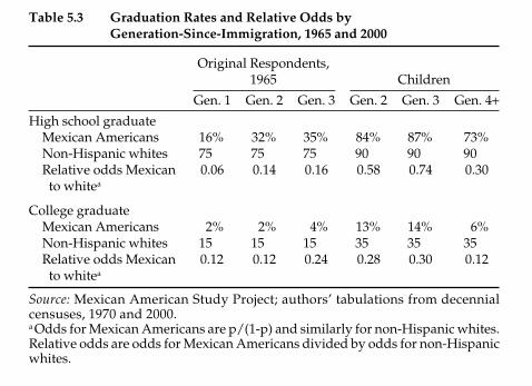
An odds ratio of .06 for high school graduates among first-generationrespondents in 1965, for example, indicates that the odds that a Mexicanimmigrant graduated from high school is about 6 percent (.06) of the oddsthat a white graduated. Table 5.3 shows that the odds ratios of graduatingfrom high school vis-à-vis a non-Hispanic white American are lower amongimmigrants than those born in the United States, as expected. The ratiosincrease with generation-since-immigration, except in the case of fourth-generation children, who have lower odds ratios than both second- andthird-generation children. The odds ratios for children are greater than thoseof the original respondents, indicating a shrinking racial gap in educationalattainment from the original respondents in 1965 to their children in 2000.
Improvement rates of high school graduation are greater than those forcollege graduation. The bold lines in figure 5.4 illustrate the gap betweenMexicans and non-Hispanic whites for high school and college completionfrom the second-generation original respondents to their third-generationchildren, using the odds ratios. The dotted lines show the same gap for thethird-generation respondents, connected to the third-generation children,which one could argue is a fairer comparison. Despite three decades ofuniversity-based affirmative action, college education relative to whiteshas improved from 12 percent odds in the second generation in 1965 to
Education 115
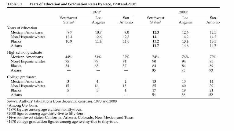
Table 5.1 Years of Education and Graduation Rates by Race, 1970 and 2000a
1970b 2000c
Southwest Los San Southwest Los San Statesd Angeles Antonio Statesd Angeles Antonio
Years of educationMexican Americans 9.7 10.7 9.0 12.3 12.6 12.5Non-Hispanic whites 12.3 12.6 12.3 14.1 14.2 14.2Blacks 10.9 11.4 11.0 13.2 13.4 13.5Asians — — — 14.7 14.6 14.7
High school graduateMexican Americans 44% 51% 37% 74% 76% 77%Non-Hispanic whites 75 79 74 90 94 95Blacks 54 63 57 84 84 89Asians — — — 95 95 93
College graduatee
Mexican Americans 3 4 2 13 13 14Non-Hispanic whites 15 16 15 35 40 39Blacks 5 5 4 17 19 21Asians — — — 54 56 52
Source: Authors’ tabulations from decennial censuses, 1970 and 2000.a Among U.S. born.b 1970 figures among age eighteen to fifty-four.c 2000 figures among age thirty-five to fifty-four.d Five southwest states: California, Arizona, Colorado, New Mexico, and Texas.e 1970 college graduation figures among age twenty-five to fifty-four.
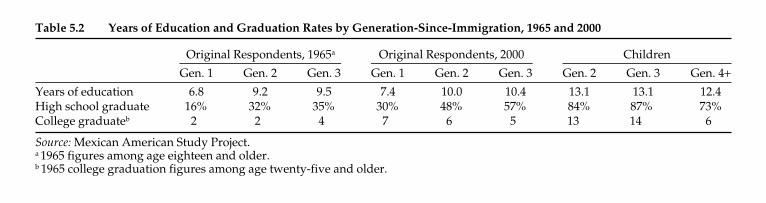
Table 5.2 Years of Education and Graduation Rates by Generation-Since-Immigration, 1965 and 2000
Original Respondents, 1965a Original Respondents, 2000 Children
Gen. 1 Gen. 2 Gen. 3 Gen. 1 Gen. 2 Gen. 3 Gen. 2 Gen. 3 Gen. 4+Years of education 6.8 9.2 9.5 7.4 10.0 10.4 13.1 13.1 12.4High school graduate 16% 32% 35% 30% 48% 57% 84% 87% 73%College graduateb 2 2 4 7 6 5 13 14 6
Source: Mexican American Study Project.a 1965 figures among age eighteen and older.b 1965 college graduation figures among age twenty-five and older.
114 Generations of Exclusion
Our data also allowed us to investigate the educational achievementof the grandchildren of the original respondents, enabling us to distin-guish a fifth generation-since-immigration. We did not directly interviewthe children of the child sample, but instead asked the children of the orig-inal respondents about their own children’s education level. Because manyof these children were not yet adults and thus had not completed theireducation, we limited our investigation to high school graduation rates forthose twenty years old and older. Figure 5.3 shows that these grand-children of the original respondents, who are third to fifth generation,seemed to be doing no better than their parents. By this time, the third,fourth, and fifth generation were performing equally, with no significantdifferences among them. In the third generation, 85 percent had graduatedfrom high school, versus 84 percent of the fourth generation and 81 percentof the fifth generation.19
To demonstrate the gap in educational achievement between MexicanAmericans and whites, we computed odds ratios. These are based on datafrom table 5.1 for whites and table 5.2 for Mexican Americans, and arepresented in table 5.3. We calculate the odds that both groups graduatedfrom high school (by dividing the proportion that graduated by the pro-portion that did not graduate or p/1-p). We then divide the odds forMexican Americans by the odds for whites to yield odds ratios (also referredto as relative odds). These are presented on the third and sixth rows oftable 5.3. Odds ratios have desirable mathematical properties for measuring
Table 5.3 Graduation Rates and Relative Odds by Generation-Since-Immigration, 1965 and 2000
Original Respondents,1965 Children
Gen. 1 Gen. 2 Gen. 3 Gen. 2 Gen. 3 Gen. 4+High school graduate
Mexican Americans 16% 32% 35% 84% 87% 73%Non-Hispanic whites 75 75 75 90 90 90Relative odds Mexican 0.06 0.14 0.16 0.58 0.74 0.30
to whitea
College graduateMexican Americans 2% 2% 4% 13% 14% 6%Non-Hispanic whites 15 15 15 35 35 35Relative odds Mexican 0.12 0.12 0.24 0.28 0.30 0.12to whitea
Source: Mexican American Study Project; authors’ tabulations from decennial censuses, 1970 and 2000.a Odds for Mexican Americans are p/(1-p) and similarly for non-Hispanic whites.Relative odds are odds for Mexican Americans divided by odds for non-Hispanicwhites.
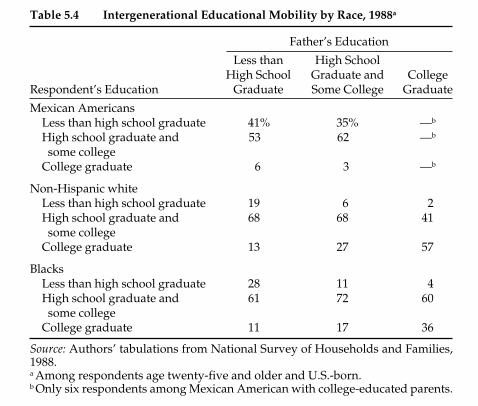
Table 5.4 Intergenerational Educational Mobility by Race, 1988a
Father’s Education
Less than High SchoolHigh School Graduate and College
Respondent’s Education Graduate Some College Graduate
Mexican AmericansLess than high school graduate 41% 35% —b
High school graduate and 53 62 —b
some collegeCollege graduate 6 3 —b
Non-Hispanic whiteLess than high school graduate 19 6 2High school graduate and 68 68 41some college
College graduate 13 27 57
BlacksLess than high school graduate 28 11 4High school graduate and 61 72 60some college
College graduate 11 17 36
Source: Authors’ tabulations from National Survey of Households and Families,1988.a Among respondents age twenty-five and older and U.S.-born.b Only six respondents among Mexican American with college-educated parents.
Education 117
They have the knowledge and the time to read frequently to their childrenand expose them to other cultural advantages. They have higher educa-tional expectations and are role models for their children. They are morelikely to know the pathways to educational success, can better navigatecomplex school systems, and manage their education in numerous otherways.20 The positive effect of parental education on children’s educationis thus not surprising.
The conceptual origin of this view is status attainment theory, whichhas become a mainstay of American sociology. The first stage of thismodel posits that educational or status attainment of any kind is largelytransmitted from parents to children.21 The model also recognizes thatthe rate of transmission may vary by race and ethnicity and other factors,such as generation-since-immigration.22 Modern assimilation theory23
draws largely from the status attainment model in that it predicts that thechildren of immigrants with high levels of education will assimilate fasterthan those whose parents have less education, though it also expects thatfor most descendants of less educated immigrants, education will improvein the second generation and again in the third.

Table 5.5 Intergenerational Educational Mobility by Generation-Since-Immigration, 2000
Father’s Education
Less than High School High School Graduate and College
Child’s Education Graduate Some College Graduate
Generation 2Less than high school 18% 10% —a
graduateHigh school graduate 70 79 —a
and some collegeCollege graduate 12 10 —a
Generation 3+Less than high school 24 10 0graduate
High school graduate and some 71 70 81college
College graduate 6 20 18
Source: Mexican American Study Project.a Only nine respondents among generation 2 with college-educated parents.
Table 5.6 Parental Status and Resources and Years of Education, 2000
Years of Relationship Education with Educationa
Father’s education 0.10***Nine or less years 12.4More than nine years 13.5
Mother’s education 0.08***Nine or less years 12.5More than nine years 13.4
Parents’ income 0.06*$6,000 or less 12.5More than $6,000 13.4
Parent was homeowner 0.32†Renter 12.5Owner 13.3
Number of siblings −0.08*One to three siblings 13.5More than three siblings 12.7
Source: Mexican American Study Project.a Linear regression run. Unstandardized coefficients presented. Child sample ana-lyzed. Adjusted for sibling clustering. Father’s education, mother’s education,parents’ income, and number of siblings entered as continuous variables in regres-sion model. See appendix B, table B.3 for full model.†p<.10, *p<.05, ***p<.001

Education 121
not worse than those of second-generation children. Portes and Rumbautalso contended that the lack of bilingualism among the third generation-since-immigration may be a further language disadvantage, which theyclaimed reduces cognitive abilities overall and lowers the self-esteem ofMexican Americans.
We test these hypotheses using two variables: whether parents wereSpanish monolingual and whether children were bilingual while growingup. Although our sample is primarily U.S.-born, there were Spanish mono-lingual immigrant parents in our study. The children of Spanish mono-linguals had 12.6 years of schooling in contrast to 13.0 for the children ofthose who knew English, whether bilingual or monolingual. Childrenwho grew up hearing Spanish had 13.0 years of education and those whodid not had 12.8 years. However, once we control for other key factors,such as generation-since-immigration and parental status, there are nostatistically significant relationships between language and educationaloutcomes, as the second column of table 5.7 reveals.
A common conception is that the low education of Mexican Americansis due to their parents’ low expectations or aspirations. However, Schneiderand her colleagues, Portes and Rumbaut, and others recognize that one ofthe few advantages of Mexican-origin parents is their high educationalaspirations and expectations.26 Based on our data, 65 percent of the parentsreported in 1965 that they would have liked their children to graduate fromcollege. Thus, we test whether having these aspirations has any effect onthe eventual educational attainment of their children. The children whoseparents wanted them to finish college appear to have somewhat highereducational outcomes—13.3 years of schooling for those who had these
Table 5.7 Cultural Deficits and Years of Education, 2000
Years of Relationship Education with Educationa
Parent is Spanish monolingual −0.18Not Spanish monolingual 13.0Spanish monolingual 12.6
Parent spoke Spanish to child 0.20Did not speak Spanish to child 13.0Spoke Spanish to child 12.8
Parent’s college aspirations for children 0.04Had less than college aspirations 12.7Had college aspirations 13.3
Source: Mexican American Study Project.a Linear regression run. Unstandardized coefficients presented. Child sample ana-lyzed. Adjusted for sibling clustering. See appendix B, table B.3 for full model.
122 Generations of Exclusion
higher aspirations compared to 12.7 to those who did not (see table 5.7).However, this relationship is not statistically significant in the multivari-ate analysis. We suggest that higher educational aspirations are relatedto parent’s own level of schooling, which washes out the parental aspi-rations variable in the multivariate analysis. Parents with higher educa-tional aspirations for their children did not have children who go on tohave higher educations, once we control for other factors.
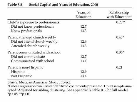
Social CapitalSocial capital as we use it refers roughly to the advantages that some indi-viduals have because of their or their family’s location in, or relation to,social networks.27 Although definitions of social capital are varied, theygenerally refer to the idea that who one knows is beneficial to gettingahead. In our study, our social capital indicators reflect whether respon-dents were exposed to professionals while growing up, whether theyattended church weekly, whether parents communicated with the school,and whether a parent was not Hispanic. The bivariate and multivariateresults in table 5.8 indicate that our first indicator of social capital is stronglyand positively related to children’s educational outcomes. Children whoknew “doctors, lawyers or teachers,” as we asked in the survey, ended upwith more education. We suspect that such persons provided the child
Table 5.8 Social Capital and Years of Education, 2000
Years of Relationship Education with Educationa
Child’s exposure to professionals 0.23**Did not know professionals 12.7Knew professionals 13.3
Parent attended church weekly 0.45*Did not attend church weekly 12.6Attended church weekly 13.3
Parent communicated with school 0.36*Did not communicate 12.7Communicated with school 13.1
Parent is non-Hispanic 0.21Hispanic 12.9Not Hispanic 13.4
Source: Mexican American Study Project.a Linear regression run. Unstandardized coefficients presented. Child sample ana-lyzed. Adjusted for sibling clustering. See appendix B, table B.3 for full model.*p<.05, **p<.01
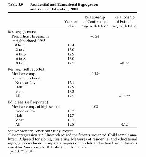
Table 5.9 Residential and Educational Segregation and Years of Education, 2000
Relationship RelationshipYears of of Continuous of Extreme
Educ. Seg. with Educ.a Seg. with Educ.
Res. seg. (census)Proportion Hispanic in −0.24neighborhood, 19650 to .2 13.4.2 to .4 13.0.4 to .6 12.9.6 to .8 13.0.8 to 1.0 12.5 –0.22
Res. seg. (self reported)Mexican comp. −0.13†of neighborhoodNone or few 13.1Half 12.9Most 13.3All 12.5 –0.50**
Educ. seg. (self reported)Mexican comp. of high school 0.03
None or few 13.2Half 12.7Most 13.1All 12.8 0.12
Source: Mexican American Study Project.a Linear regression run. Unstandardized coefficients presented. Child sample ana-lyzed. Adjusted for sibling clustering. Measures of residential and educationalsegregation included in separate regression models and entered as continuousvariables. See appendix B, table B.3 for full model. †p<.10; **p<.01
124 Generations of Exclusion
neighborhoods, thus should attend more integrated schools and seetheir children’s education improve.
The view that segregation continues to drive the inferior education ofLatino and African American children remains popular today. GaryOrfield and Jonathon Kozol, perhaps the two most well-known advocatesof this view, have focused much attention on the role of segregation as themajor contributor to the lowly state of minority education.32 They arguethat segregated schools have lower levels of funding, less experiencedteachers, and poorer facilities in comparison with mostly white schools.Moreover, students in such schools are exposed to more violence.33
We measure segregation in table 5.9 as the presence of other Hispanicsin the neighborhood or the school. Specifically we use three measures:
Education 127
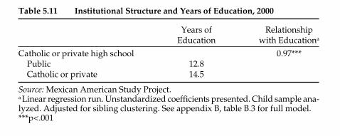
InstitutionalColeman and others have long argued that Catholic schools providesuperior education in part because they have higher expectations forall students and create a more disciplinary climate, which promotesbetter student behavior.37 These findings of better educational outcomesfor Catholic schools are based mostly on quantitative evidence in the1980s using national data sets. These studies also conclude that Catholicschools place a greater emphasis on core academic subjects, require morehomework, enable a common set of values based on religious beliefs, cre-ate a greater sense of community due to smaller school size, and allow forgreater teacher and counselor involvement. More importantly, ThomasHoffer, Andrew Greeley, and James Coleman found that achievementdifferences among whites, blacks, and Hispanics were smaller in Catholicschools than public ones and that racial differences were especially smallby the senior year.38 At least one study noted the especially positive effectof Catholic school for Hispanics.39 Several qualitative studies show thatAfrican Americans also benefit from a Catholic school education.40
We also find that attending Catholic schools had a very strong effect onthe education of children, as table 5.11 reveals. Specifically, the 12 percentof the child sample who began their high school educations in Catholic orprivate schools (89 percent of these were Catholic) eventually completedclose to two (1.7) more years of school than those who began high school inpublic school. In the multivariate analysis, those attending Catholic schoolshave roughly one more year of schooling than their public school counter-parts (see table 5.11). Thus, the very large bivariate difference, while partlyexplained by the controls such as parental status, appears to be mostly fromactual differences between Catholic and public schools.
This finding is consistent with the substantial body of research showinga Catholic–private school bonus, despite extensive methodological debates
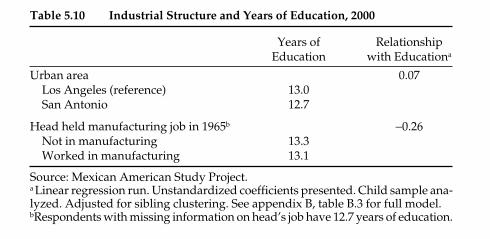
Table 5.10 Industrial Structure and Years of Education, 2000
Years of Relationship Education with Educationa
Urban area 0.07Los Angeles (reference) 13.0San Antonio 12.7
Head held manufacturing job in 1965b −0.26Not in manufacturing 13.3Worked in manufacturing 13.1
Source: Mexican American Study Project.a Linear regression run. Unstandardized coefficients presented. Child sample ana-lyzed. Adjusted for sibling clustering. See appendix B, table B.3 for full model.bRespondents with missing information on head’s job have 12.7 years of education.
128 Generations of Exclusion
about selectivity.41 In particular, much of that research has been challengedby the argument that Catholic and private schools pick the best and mostmotivated students and particularly those whose parents can afford topay. Enrollment in a Catholic school probably also reflects the willingnessof some parents to sacrifice limited incomes to attend these schools.
Recent research, however, which carefully controls for selectivity, sup-ports the contention of better outcomes overall for Catholic school stu-dents,42 especially for minority and inner-city children who often livewhere public school education is poor.43 Our findings also show that asubstantial Catholic–private school bonus seems to persist beyond parentalfinancial or other types of advantages since we control for a host of parentalsocio-economic status and family resource characteristics. Unfortunately,Mexican Americans have not had nearly as much access to Catholic edu-cation that Irish and Italian immigrants and their descendants had, whichwas largely responsible for those groups’ mobility.44
Skin Color, Gender, and AgeTable 5.12 shows that there are no real differences in educational attain-ment related to skin color, gender, and age in the bivariate analysis. Exceptfor marginally significant differences by gender, there are no differences inthe regression analysis either. The results for gender suggest that MexicanAmerican women have slightly less education than men. Jean Phinney andJuana Flores argue that such differences reflect parental expectations thatboys succeed in mainstream society and girls are socialized for moredomestic tasks.45 We also expected that years of education would haveimproved over the twenty-year age range among the children in our sam-ple. However, we find no such difference.
Despite previous findings showing that darker skin color predicts lowereducation levels among Mexican Americans,46 our findings in table 5.12show that those with lighter skin color did no better than their counter-parts. There is also no skin color effect when we examine skin color as a
Table 5.11 Institutional Structure and Years of Education, 2000
Years of RelationshipEducation with Educationa
Catholic or private high school 0.97***Public 12.8Catholic or private 14.5
Source: Mexican American Study Project.a Linear regression run. Unstandardized coefficients presented. Child sample ana-lyzed. Adjusted for sibling clustering. See appendix B, table B.3 for full model.***p<.001
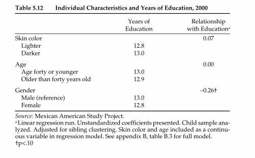
continuum—that is using five or seven categories (analysis not shown).This may reflect a changing effect of skin color, which has been observedfor African Americans,47 or perhaps an effect of place. In places whereMexican Americans comprise a large proportion of the population, like LosAngeles or San Antonio, Mexican children in schools may be readily iden-tified on the basis of other characteristics, such as surname or peer associa-tions, so that skin color is only a secondary marker of race or ethnicity.
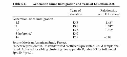
Generation-Since-ImmigrationWe now come back to generation-since-immigration, our main independentvariable of concern. The bivariate results we presented in table 5.2 showincreases in education from the first generation to their children. Thereare few gains from the second to the third generation across family genera-tions or generation-since-immigration, though the fourth generation hadnotably lower years of education than the other U.S.-born. The bivariateresults in the first column of table 5.13 reflect this pattern for the child sam-ple. However, as the multivariate analysis thus far has revealed, suchresults may be due to the effect of other variables that may be similarly cor-related with years of education. We thus examine the independent effectsof generation-since-immigration among the children, as we did for otherfactors.
We further disaggregate our sample into five generation-since-immigration (1.5, 2, 2.5, 3 and 4), which we define on the basis of the placeof birth or generation of both parents. The creation of this variable isdescribed in chapter 3 (see table 3.10). Because the experience of the
Education 129
Table 5.12 Individual Characteristics and Years of Education, 2000
Years of RelationshipEducation with Educationa
Skin color 0.07Lighter 12.8Darker 13.0
Age 0.00Age forty or younger 13.0Older than forty years old 12.9
Gender −0.26†Male (reference) 13.0Female 12.8
Source: Mexican American Study Project.a Linear regression run. Unstandardized coefficients presented. Child sample ana-lyzed. Adjusted for sibling clustering. Skin color and age included as a continu-ous variable in regression model. See appendix B, table B.3 for full model.†p<.10
second generation may be quite heterogeneous, we further divide it intothree groups: the 1.5 generation, which refers to persons who are immi-grants but immigrated with their parents when they were children; the sec-ond generation, which we define for the regression analysis (in this and allsubsequent chapters) as the U.S.-born children of two immigrant parents;and the 2.5 generation, which is also U.S.-born with only one immigrantparent. The 1.5 generation were children at the time of immigration, whofinished who schooling in the United States.
We present the regression coefficients in the second column of table 5.13and they show the additional years of schooling that children from genera-tions 1.5, two, 2.5, and four have in comparison to those from generationthree. The coefficients reveal quite striking results for generation-since-immigration, when all other variables are controlled. There is a progres-sive decline in years of education for each subsequent generation-since-immigration in the multivariate analysis. Immigrant children who came tothe United States at a young age with their parents, the so-called 1.5 gener-ation, have the highest levels of schooling, once all the other variables arecontrolled. They have about a half-year greater schooling than the secondgeneration, who have a half-year more schooling than the 2.5 generation,who in turn have a half-year more schooling than the third generation. Thethird and fourth generations have the least schooling and there is no differ-ence between them. In terms of statistical significance, the 1.5 and the sec-ond generation are significantly better educated than the third generationat the .05 level, the 2.5 generation is marginally better educated than thethird at a marginally significant level (.10) and there are no statistically sig-nificant differences between the third and fourth generations.48 Moreover,the generational differences in the multivariate analysis (column two) areactually greater than in the bivariate analysis (column one). Therefore, con-trolling for various alternative explanations actually increases differencesby generation.49 Thus, our results show that educational attainment
130 Generations of Exclusion
Table 5.13 Generation-Since-Immigration and Years of Education, 2000
Years of RelationshipEducation with Educationa
Generation-since-immigration1.5 13.3 1.46**2 13.1 0.94**2.5 13.2 0.40†3 (reference) 13.04+ 12.5 −0.08
Source: Mexican American Study Project.a Linear regression run. Unstandardized coefficients presented. Child sample ana-lyzed. Adjusted for sibling clustering. See appendix B, table B.3 for full model.†p<.10, **p<.01
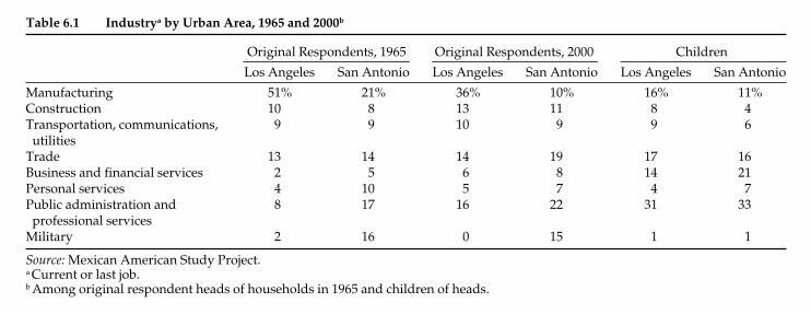
Table 6.1 Industrya by Urban Area, 1965 and 2000b
Original Respondents, 1965 Original Respondents, 2000 Children
Los Angeles San Antonio Los Angeles San Antonio Los Angeles San Antonio
Manufacturing 51% 21% 36% 10% 16% 11%Construction 10 8 13 11 8 4Transportation, communications, 9 9 10 9 9 6utilities
Trade 13 14 14 19 17 16Business and financial services 2 5 6 8 14 21Personal services 4 10 5 7 4 7Public administration and 8 17 16 22 31 33professional services
Military 2 16 0 15 1 1
Source: Mexican American Study Project.a Current or last job.b Among original respondent heads of households in 1965 and children of heads.
jobs. For the children, however, dependence on government jobs hadequalized in the two urban areas. Most strikingly, military employment inSan Antonio decreased from 16 percent for original respondents to 1 per-cent among the children.
Earnings and Income
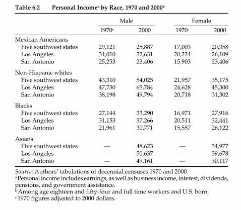
Grebler and his colleagues documented that personal income levels14 forMexican Americans were significantly lower than among non-Hispanicwhites—a gap of 57 percent—in the five southwestern states.15 The gapwas also greater in Texas than in California—79 percent and 50 percentrespectively. Grebler also showed that Mexicans had slightly higher incomethan nonwhites, which at the time of the original study was almostentirely African American. Data presented in table 6.2 show that incomeinequality between Mexican Americans and whites worsened from 1970levels.
To get a sense of how racial-ethnic groups have fared economically overtime, table 6.2 uses 1970 and 2000 census data to calculate average personal
Economic Status 139
Table 6.2 Personal Incomea by Race, 1970 and 2000b
Male Female
1970c 2000 1970c 2000
Mexican AmericansFive southwest states 29,121 25,887 17,003 20,358Los Angeles 34,010 32,631 20,224 26,109San Antonio 25,253 23,406 15,903 23,406
Non-Hispanic whitesFive southwest states 43,310 54,025 21,957 35,175Los Angeles 47,730 65,784 24,628 45,300San Antonio 38,198 49,794 20,718 31,302
BlacksFive southwest states 27,144 33,290 16,971 27,916Los Angeles 31,153 37,266 20,511 32,441San Antonio 21,961 30,771 15,557 26,122
AsiansFive southwest states — 48,623 — 34,977Los Angeles — 50,637 — 39,678San Antonio — 49,161 — 30,117
Source: Authors’ tabulations of decennial censuses 1970 and 2000.a Personal income includes earnings, as well as business income, interest, dividends,pensions, and government assistance.b Among age eighteen and fifty-four and full time workers and U.S. born.c 1970 figures adjusted to 2000 dollars.

Table 6.3 Earnings and Income by Generation-Since-Immigration, 1965 and 2000
Original Respondents, 1965a Original Respondents, 2000 Children
Gen. 1 Gen. 2 Gen. 3 Gen. 1 Gen. 2 Gen. 3 Gen. 2 Gen. 3 Gen. 4+Personal earningsb $25,556 $29,243 $29,319 $25,923 $29,748 $29,151 $36,343 $37,615 $30,559Family incomec $32,404 $35,654 $35,537 $25,445 $28,442 $28,952 $53,174 $53,634 $43,891Below povertyd 25% 20% 20% 38% 37% 38% 17% 14% 21%High family incomee 11 13 12 10 14 16 47 47 36
Source: Mexican American Study Project.a 1965 figures adjusted to 2000 dollars.b Personal earnings includes wages and business income; among workers.c Family income based on husband’s and wife’s income and includes personal income, interest, dividends, pensions, and governmentassistance.d Below poverty based on family income using government thresholds (based on family size and composition).e High family income more than $50,000 in 2000 dollars.
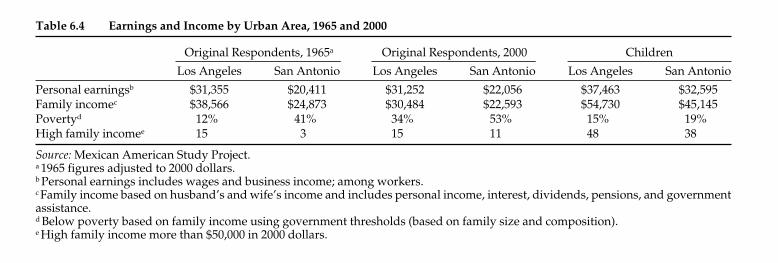
Table 6.4 Earnings and Income by Urban Area, 1965 and 2000
Original Respondents, 1965a Original Respondents, 2000 Children
Los Angeles San Antonio Los Angeles San Antonio Los Angeles San Antonio
Personal earningsb $31,355 $20,411 $31,252 $22,056 $37,463 $32,595Family incomec $38,566 $24,873 $30,484 $22,593 $54,730 $45,145Povertyd 12% 41% 34% 53% 15% 19%High family incomee 15 3 15 11 48 38
Source: Mexican American Study Project.a 1965 figures adjusted to 2000 dollars.b Personal earnings includes wages and business income; among workers.c Family income based on husband’s and wife’s income and includes personal income, interest, dividends, pensions, and governmentassistance.d Below poverty based on family income using government thresholds (based on family size and composition).e High family income more than $50,000 in 2000 dollars.

Table 6.5 Occupational Distribution and Occupational Index by Generation-Since-Immigration, 1965 and 2000
Original Respondents, 1965 Original Respondents, 2000 Children
Gen. 1 Gen. 2 Gen. 3 Gen. 1 Gen. 2 Gen. 3 Gen. 2 Gen. 3 Gen. 4+Occupational distribution
Professional or manager 8% 10% 7% 12% 14% 16% 28% 26% 18%Technical or administrative 10 15 20 21 26 27 38 35 32
Total white collar 18 25 27 33 40 43 66 60 50
Service 5 12 4 13 19 19 12 10 17
Production or repair 20 24 28 19 16 17 10 16 20Operatives or laborer 57 40 42 35 24 21 12 14 14
Total blue collar 77 64 60 54 40 38 22 30 34
Mean occupational indexa 28.5 29.9 30.5 28.0 30.2 31.5 36.4 36.1 32.1
Source: Mexican American Study Project.a Occupational index ranges from zero to one-hundred and a composite of education and wages for workers in detailed occupationalcategories calculated separately for men and women.
our respondents. These results make it quite apparent that intergenera-tional occupational status has improved from the original respondents totheir children. This reflects a long-term change in occupations for the UnitedStates overall. We note that the occupational index of the original respon-dents remained almost exactly the same between 1965 and 2000, suggestingalmost no occupational mobility during the careers of original respondents,though intergenerational occupational mobility was considerable.
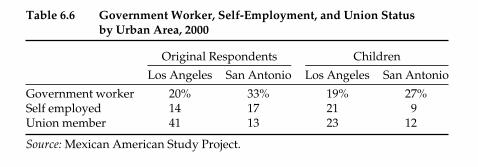
Additional characteristics—such as government employment, self-employment, and union membership—tell us about the quality of respon-dent jobs. However, such characteristics may vary widely betweenCalifornia and Texas because of the very different labor markets and legalenvironments of the two locations. We present data on these characteris-tics by urban area in table 6.6. Just as Grebler and his colleagues showedthat Mexican Americans in Texas in 1965 were more likely to hold gov-ernment jobs than those in California, we find that both original respon-dents and their children in San Antonio were also more likely to work inor recently hold government jobs in 2000.21 Self-employment was rela-tively low for original respondents in both Los Angeles (17 percent) andSan Antonio (14 percent), and was lower still for their children. Last, weobserve that fully 41 percent of original respondents in Los Angeles butonly 13 percent of those raised in San Antonio were union members. Thisis consistent with the fact that Texas is a right-to-work state.22 For the chil-dren, the percentages of unionized workers in our sample fell in LosAngeles, reflecting both a national and local decline in union membershipand a movement to white-collar jobs, where unions tend to be less preva-lent.23 In San Antonio, rates of unionization remained the same for bothoriginal respondents and their children.
Homeownership and Wealth
Recent studies have shown that whereas the average incomes of AfricanAmericans are less than those for whites, differences in wealth are huge.24
Oliver and Shapiro, for example, show that median income among African
148 Generations of Exclusion
Table 6.6 Government Worker, Self-Employment, and Union Status by Urban Area, 2000
Original Respondents Children
Los Angeles San Antonio Los Angeles San Antonio
Government worker 20% 33% 19% 27%Self employed 14 17 21 9Union member 41 13 23 12
Source: Mexican American Study Project.

Table 6.7 Homeownership and Wealth by Generation-Since-Immigration, 1965 and 2000
Original Respondents, 1965 Original Respondents, 2000 Children
Gen. 1 Gen. 2 Gen. 3 Gen. 1 Gen. 2 Gen. 3 Gen. 2 Gen. 3 Gen. 4+Owns own home 54% 55% 47% 73% 73% 65% 59% 58% 49%Owns more than one home —a —a —a 22 22 23 14 12 10Net worthb —a —a —a $131,122 $111,582 $132,478 $48,424 $44,617 $38,364
Source: Mexican American Study Project.a Data not collected in 1965 survey.b Net worth based on equity in home(s) and financial assets minus debts.

Table 6.8 Homeownership and Wealth by Urban Area, 1965 and 2000
Original Respondents, 1965 Original Respondents, 2000 Children
Los Angeles San Antonio Los Angeles San Antonio Los Angeles San Antonio
Owns own home 43% 65% 69% 77% 53% 64%Owns more than one home —a —a 22 26 13 15Net worthb —a —a $141,302 $72,694 $51,711 $40,269
Source: Mexican American Study Project.a Data not collected in 1965 survey.b Net worth based on equity in home(s) and financial assets minus debts.

parents’ education, income, and homeownership had a highly signi-ficant effect on education, these variables do not directly affect socio-economic status.32 Instead, family background affects socioeconomicstatus through the child’s education, which fits well within the statusattainment model.
Despite our expectations, variables such as living in San Antonio or LosAngeles and the extent of ethnic isolation (proportion Hispanics in neigh-borhood) had no effect on socioeconomic status (as shown in the full modelin table B.4 in appendix B). Those who completed the interview by tele-phone, however, had significantly higher earnings, incomes, and net worth.This effect is partly residential because many of the telephone interviewswere with respondents who had moved away from either the Los Angelesor the San Antonio area, though in some cases we simply could not arrangein-person interviews for those who had not moved. Thus, these results sug-gest that Mexican Americans who left Los Angeles or San Antonio wereable to secure higher earnings, income, and wealth.
Interestingly, generation-since-immigration is not significantly relatedto socioeconomic status. The prediction posed by assimilation theorythat socioeconomic status should increase with generational status wasnot supported by our regression, just as it had not been shown in thedescriptive tables. There seems, however, to be minor though not sig-nificant or consistent effects suggesting slight downward assimilation on
Economic Status 153
Table 6.9 Key Determinants of Socioeconomic Status, 2000a
Occupational Earnings Income Net WorthStatus (Dollars) (Dollars) (Dollars)
Generation-since-immigration (ref: 3)1.5 0.57 −354 5,900 11,7792 0.30 −4,418 −2,584 13,3722.5 −0.76 −2,324 −630 3424+ −1.16 −3,663 −777 782
Education 2.99*** 4,043*** 6,177*** 8,977***Telephone interview 7,479** 7,816* 25,650*(2000)
Work experienceb 240*Ageb 2,917***Female −1,2895***
Source: Mexican American Study Project.a Only significant or substantive variables presented. Linear regression run. Un-standardized coefficients presented. Child sample analyzed. Adjusted for siblingclustering. See appendix B, table B.4 for full model.b Age and work experience not included in model together because highly correlated.* p<.05, **p<.01, ***p<.001
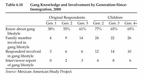
Similarly, involvement in gangs was greatest among the U.S.-bornand persisted, if not actually increased, well into the fourth generation.Among the original respondents, the greatest percentage having a fam-ily member involved in the gang lifestyle was among the third genera-tion (14 percent). Among the child generation, the fourth generationwas the most involved (26 percent). We reach similar conclusions regard-ing whether the respondent was involved in the gang lifestyle. The latergenerations are the most involved, but their participation is not signifi-cantly different from the second and third generations. Finally, inter-viewers were given some training in being attentive to gang tattoos,clothing, and posture that might suggest involvement in gangs or thegang lifestyle. We recognize substantial subjectivity on this measure.Our interviewing staff found that none of the immigrant generationshowed any signs of gang affiliation and that only 2 to 3 percent amongthe second and third generation of the original respondents did. For thechildren’s generation, interviewers identified 4 percent of the secondgeneration-since-immigration as gang-affiliated and 6 to 8 percent of thethird and fourth generation.
Conclusions
Our findings show a consistent lack of economic progress acrossgenerations-since-immigration. Among the child sample, there is noeconomic assimilation, while there are indications of slight economicassimilation for the original respondents. Indeed, our statistical analysisshows that generation-since-immigration has no significant effects on
Economic Status 155
Table 6.10 Gang Knowledge and Involvement by Generation-Since-Immigration, 2000
Original Respondents Children
Gen. 1 Gen. 2 Gen. 3 Gen. 2 Gen. 3 Gen. 4+Know about gang 38% 55% 61% 77% 65% 65%lifestyle
Family member 4 9 14 24 22 26involved in gang lifestyle
Respondent involved 3 6 6 12 14 10in gang lifestyle
Interviewer report 0 2 3 4 8 6of gang lifestyle
Source: Mexican American Study Project.

162 Generations of Exclusion
evenly represented across an urban neighborhoods in respect to eachother. It is easily interpretable because the value represents the minimumpercentage of each of the compared groups, such as Hispanics and non-Hispanic whites, that would have to exchange residences so that eachcensus tract had the same racial composition as the entire metropolitanarea. Thus, the value is completely independent of an urban area’s racialcomposition. The number varies from 0, which represents complete inte-gration, to 100, which represents complete segregation. Neighborhoods,for the purposes of these indexes, are represented by census tracts, whichaverage about 5,000 people in the U.S. Census. Low levels of segregationcharacterize the descendants of Europeans14 and high levels characterizeAfrican Americans.15
The results for dissimilarity show that values for Hispanic-white segre-gation (Hispanics in Los Angeles and San Antonio are primarily MexicanAmericans) vary from 47 to 64. These numbers put Mexican American segregation at the moderate level, though sometimes approaching theextreme.16 Most interesting are the trends from 1960 to 2000, which are verynearly diametrically opposed in the two urban areas. Los Angeles’ segre-gation increased each decade, with the exception of 1970, whereas SanAntonio’s decreased. San Antonio segregation in 1960 looks like LosAngeles segregation in 2000. Although we would expect a decrease in seg-regation since 1960 in response to increasing protections against discrimi-nation in housing and greater mobility afforded to Mexican Americans
Table 7.1 Residential Segregation Between Hispanics and Non-HispanicWhites, 1960 to 2000
1960a 1970b 1980c 1990d 2000d
Dissimilarity indexLos Angeles 57 47 57 61 63San Antonio 64 59 57 54 51
Isolation indexLos Angeles — 38 55e 71 78San Antonio — 68 68e 69 70
Source: Grebler, Moore and Guzmán (1970); Massey and Denton (1987); Iceland,Weinberg, and Steinmetz (2002).a 1960 data from Grebler, Moore and Guzmán (1970).b 1970 data from Massey and Denton (1987).c 1980 data from Massey and Denton (1987) and Iceland, Weinberg, and Steinmetz(2002).d 1990 and 2000 data from Iceland, Weinberg, and Steinmetz (2002).e Massey and Denton (1987) and Iceland, Weinberg, and Steinmetz (2002) indexesfor isolation differ. Massey and Denton report an isolation index of 50 for LosAngeles and 67 for San Antonio while Iceland, Weinberg, and Steinmetz report60 and 70 for respective urban areas. Midpoint used.
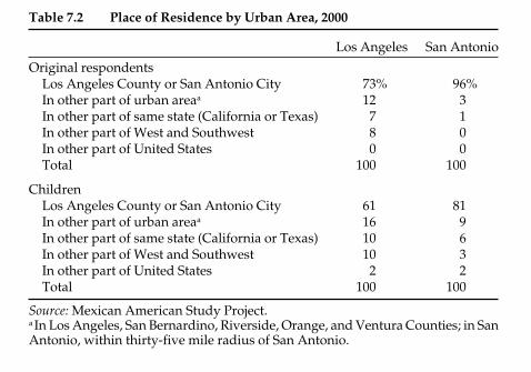
164 Generations of Exclusion
Antonio until 2000, but rose in Los Angeles over the same period. Placeswith more immigrants had greater segregation gains because immigrantsseek out ethnic neighborhoods to facilitate settlement and are limited bytheir lower incomes from moving into integrated neighborhoods.18 Thiswas surely the case for Los Angeles, which had a much higher rate ofimmigration than San Antonio.
Of course, these changes are for the overall population of whites andHispanics. Segregation in each census is not calculated for the same pop-ulation, even though the internal compositions of these populations mayhave changed. Most notably, the generational composition of the Mexican-origin population shifted greatly in Los Angeles from 1970 to 2000 withimmigration. We cannot control this with the available census data. Ourdata, however, unlike that based on the census, allow analysis of segrega-tion by generation, which we do in the following section.
Where They Live Now
Our original sample was of residents in Los Angeles County and SanAntonio City in 1965, many of whom continued to reside there in 2000though some had moved out. Before trying to understand urban segrega-tion in the two cities or among the respondents, we investigate the extentof dispersion outside of the two urban areas. Table 7.2 displays our results.The extent to which original respondents and their children migrated out
Table 7.2 Place of Residence by Urban Area, 2000
Los Angeles San Antonio
Original respondentsLos Angeles County or San Antonio City 73% 96%In other part of urban areaa 12 3In other part of same state (California or Texas) 7 1In other part of West and Southwest 8 0In other part of United States 0 0Total 100 100
ChildrenLos Angeles County or San Antonio City 61 81In other part of urban areaa 16 9In other part of same state (California or Texas) 10 6In other part of West and Southwest 10 3In other part of United States 2 2Total 100 100
Source: Mexican American Study Project.a In Los Angeles, San Bernardino, Riverside, Orange, and Ventura Counties; in SanAntonio, within thirty-five mile radius of San Antonio.
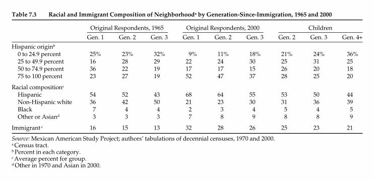
Table 7.3 Racial and Immigrant Composition of Neighborhooda by Generation-Since-Immigration, 1965 and 2000
Original Respondents, 1965 Original Respondents, 2000 Children
Gen. 1 Gen. 2 Gen. 3 Gen. 1 Gen. 2 Gen. 3 Gen. 2 Gen. 3 Gen. 4+Hispanic originb
0 to 24.9 percent 25% 23% 32% 9% 11% 18% 21% 24% 36%25 to 49.9 percent 16 28 29 22 24 30 25 31 2550 to 74.9 percent 36 22 19 17 17 15 26 20 1875 to 100 percent 23 27 19 52 47 37 28 25 20
Racial compositionc
Hispanic 54 52 43 68 64 55 53 50 44Non-Hispanic white 36 42 50 21 23 30 31 36 39Black 7 4 4 2 3 4 5 4 5Other or Asiand 3 3 3 7 8 9 8 8 9
Immigrant c 16 15 13 32 28 26 25 23 21
Source: Mexican American Study Project; authors’ tabulations of decennial censuses, 1970 and 2000.a Census tract.b Percent in each category.c Average percent for group.d Other in 1970 and Asian in 2000.
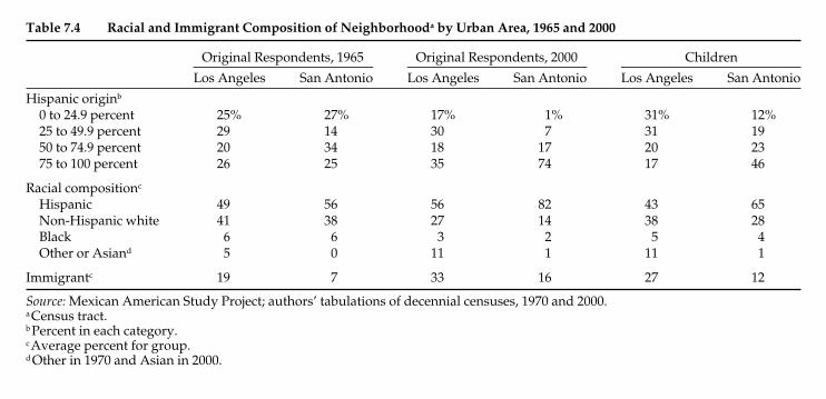
Table 7.4 Racial and Immigrant Composition of Neighborhooda by Urban Area, 1965 and 2000
Original Respondents, 1965 Original Respondents, 2000 Children
Los Angeles San Antonio Los Angeles San Antonio Los Angeles San Antonio
Hispanic originb
0 to 24.9 percent 25% 27% 17% 1% 31% 12%25 to 49.9 percent 29 14 30 7 31 1950 to 74.9 percent 20 34 18 17 20 2375 to 100 percent 26 25 35 74 17 46
Racial compositionc
Hispanic 49 56 56 82 43 65Non-Hispanic white 41 38 27 14 38 28Black 6 6 3 2 5 4Other or Asiand 5 0 11 1 11 1
Immigrantc 19 7 33 16 27 12
Source: Mexican American Study Project; authors’ tabulations of decennial censuses, 1970 and 2000.a Census tract.b Percent in each category.cAverage percent for group.dOther in 1970 and Asian in 2000.
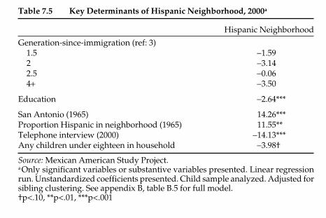
170 Generations of Exclusion
grated in 1965, it would almost certainly become more Hispanic by 2000because of immigration. An equally likely scenario is that many MexicanAmericans moved out from the barrio to more integrated suburbs or neigh-borhoods, though these also became increasingly Hispanic or immigrant.
The children from Los Angeles are likely to live in communities ethni-cally similar to those where they grew up. For instance, the average per-centage Hispanic for Los Angeles respondents in 1965 was 49 percent. Fortheir children, though there were more immigrants, it was 43 percent. Thepercentage white and percentage black remained relatively similar for theLos Angeles children, though the percentage of Asians more than doubled.For San Antonians, the presence of Anglo neighbors declined from 38 to 28percent.
Factors Affecting Residential Segregation
As with the other chapters, here we examine the independent effects ofgeneration-since-immigration and other variables on residential segrega-tion through a multivariate analysis. Residential segregation is a contin-uous dependent variable represented by the percent Hispanic in one’sneighborhood (that is, roughly speaking, the extent of residential isola-tion). We therefore run a linear regression and present the coefficients forthe statistically significant effects in table 7.5.
The results for residential segregation reveal that generation-since-immigration has no statistically significant effect, after controlling for a
Table 7.5 Key Determinants of Hispanic Neighborhood, 2000a
Hispanic Neighborhood
Generation-since-immigration (ref: 3)1.5 −1.592 −3.142.5 −0.064+ −3.50
Education −2.64***
San Antonio (1965) 14.26***Proportion Hispanic in neighborhood (1965) 11.55**Telephone interview (2000) −14.13***Any children under eighteen in household −3.98†
Source: Mexican American Study Project.a Only significant variables or substantive variables presented. Linear regressionrun. Unstandardized coefficients presented. Child sample analyzed. Adjusted forsibling clustering. See appendix B, table B.5 for full model.†p<.10, **p<.01, ***p<.001
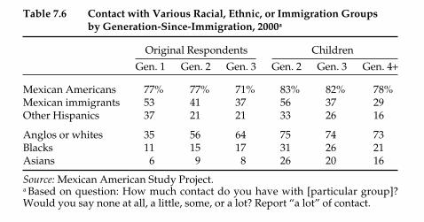
172 Generations of Exclusion
second generation had much contact with Mexican immigrants, versusonly 29 percent of their fourth-generation counterparts. We find similarlevels of contact with other Hispanics—37 percent of first-generation orig-inal respondents versus 21 percent of the third generation, and 33 percentof second-generation children versus 16 percent of the fourth generation.
For the original respondents in 2000, contact across generations-since-immigration with whites and blacks increased. The original respondentsample shows the traditional assimilation pattern of growing contact withthe dominant group, which is consistent with the findings for neighbor-hoods (shown in table 7.3). Original respondent immigrants have rela-tively little contact with African Americans and Asians, but it increaseswith generation-since-immigration, though it also reflects the greater like-lihood of traversing residential boundaries, particularly for the U.S.-born.Moreover, they are age fifty to eighty-five by the time of the second sur-vey and thus may be more likely to participate in senior activities that spanneighborhoods and are more integrated.
For the children, the extent of contact with non-Hispanic whites is nearly at the level of contact for Mexican Americans. Although many ofthe children of the original respondents continue to live in mostly Hispanicneighborhoods, they nevertheless have substantial contact with Anglos.Moreover, this contact is essentially the same across generation-since-immigration. On the other hand, contact with blacks and Asians for thechildren decreases across generation-since-immigration, which may partlyreflect the out-migration of the children from Los Angeles and San Antonio.
Because we suspect that the pattern of contact with other groups hasmuch to do with the local racial composition of Los Angeles compared toSan Antonio, we explore similar data by urban area. Table 7.7 shows thatthose living in San Antonio in 1965 and 1966 continued to have more con-
Table 7.6 Contact with Various Racial, Ethnic, or Immigration Groups by Generation-Since-Immigration, 2000a
Original Respondents Children
Gen. 1 Gen. 2 Gen. 3 Gen. 2 Gen. 3 Gen. 4+
Mexican Americans 77% 77% 71% 83% 82% 78%Mexican immigrants 53 41 37 56 37 29Other Hispanics 37 21 21 33 26 16
Anglos or whites 35 56 64 75 74 73Blacks 11 15 17 31 26 21Asians 6 9 8 26 20 16
Source: Mexican American Study Project.a Based on question: How much contact do you have with [particular group]?Would you say none at all, a little, some, or a lot? Report “a lot” of contact.
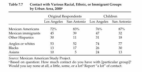
tact with other Mexican Americans than Angelenos did. This largely mir-rors the racial composition of the two cities and, for the U.S.-born MexicanAmerican population, also reflects greater residential isolation in San Antonio. On the other hand, those who grew up in Los Angeles con-tinued to have more contact with Mexican immigrants, non-MexicanHispanics, and Asians, again reflecting urban compositional differencesand especially the greater influence of mass immigration from through-out Latin America and Asia on Los Angeles since 1965. Contact withblacks was nearly the same for those growing up in each urban area.
Although the extent of contact may reflect daily interactions, it says lit-tle about the meaning or strength of these relationships. Contact mayrange from colleagues to clients to friends. Table 7.8 provides informationon the extent to which the friends of our respondents are of Mexican ori-gin. This question was asked in the original survey in 1965 and askedagain in 2000. It generally shows a diversification of friendships over timefor the original respondents and by generation-since-immigration for allrespondents in both survey years. The first row shows the percent withno or few friends of Mexican origin and overall it shows a fairly constantpattern of assimilation. In 1965, 8 percent of immigrants and 17 percentof the third-generation original respondents had no or few Mexican ori-gin friends. By 2000, these proportions had increased to 18 and 26 percent.At the same time, just over half of the immigrants (54 percent) had onlyMexican friends but by 2000 only 27 percent did. For the third generation oforiginal respondents, there was virtually no change in the roughly 20 per-cent who had only Mexican-origin friends during the thirty-five years,though by 2000 more than that had none or few.
The long-term assimilation pattern suggests gradual assimilation, buteven by the fourth generation, signs of ethnic persistence in friendships
Table 7.7 Contact with Various Racial, Ethnic, or Immigrant Groups by Urban Area, 2000a
Original Respondents Children
Los Angeles San Antonio Los Angeles San Antonio
Mexican Americans 72% 83% 76% 87%Mexican immigrants 45 39 47 32Other Hispanics 30 11 31 18
Anglos or whites 53 52 74 77Blacks 13 17 26 30Asians 10 5 24 13
Source: Mexican American Study Project.a Based on question: How much contact do you have with [particular group]?Would you say none at all, a little, some, or a lot? Report “a lot” of contact.
Interethnic Relations 173

Table 7.8 Mexican Origin Friends and Attend Latino Church by Generation-Since-Immigration, 1965 and 2000
Original Respondents, 1965 Original Respondents, 2000 Children, 2000
Gen. 1 Gen. 2 Gen. 3 Gen. 1 Gen. 2 Gen. 3 Gen. 2 Gen. 3 Gen. 4+Have Mexican friends
None or few 8% 13% 17% 18% 26% 26% 25% 33% 33%Half —a —a —a 12 22 23 26 23 24Most 38 55 63 42 30 30 29 31 29All 54 31 19 27 22 20 20 13 14
Mostly Latino congregation 87 80 71 45 39 23 39 30 31
Source: Mexican American Study Project.a Category not used in 1965 questionnaire.
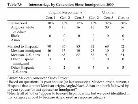
176 Generations of Exclusion
The level of exposure to other groups is known in the intermarriage liter-ature as propinquity.
Intermarriage rates are often based on the most recent marriages frommarriage vital records and thus provide useful time series for under-standing changing ethnic boundaries. They also permit making distinc-tions by age and gender. However, they are unable to indicate differencesin other variables such as generation-since-immigration. According toassimilation theory, intermarriage should increase as persons of a partic-ular ethnic ancestry are further removed from their immigrant ancestors.We calculate the amount to which our sample was intermarried based onthe current or most recent marriages for those who ever married. Table 7.9presents the race-ethnicity-immigration characteristics of the respon-dents’ current or most recent spouse in 2000 for the original respondentsand their children.
Table 7.9 shows that extent of intermarriage increases over generation-since-immigration. If we consider intermarriage as marriage to a non-Hispanic, only 10 percent of the immigrant original respondents wereintermarried, versus 17 percent of the third generation, and 15 percent ofthe second generation. Among the child sample, 18 percent of the secondgeneration, 32 percent of the third generation, and 38 percent of the fourth
Table 7.9 Intermarriage by Generation-Since-Immigration, 2000a
Original Respondents Children
Gen. 1 Gen. 2 Gen. 3 Gen. 2 Gen. 3 Gen. 4+Intermarried 10% 15% 17% 18% 32% 38%
Anglo or white 9 15 16 16 30 36or otherb
Black 0 0 0 0 0 0Asian 1 0 1 2 1 2
Married to Hispanic 90 85 83 82 68 62Mexican immigrant 46 17 10 23 10 3Mexican, U.S. born 41 65 67 53 51 54Other Hispanic 3 1 1 3 0 0immigrant
Other Hispanic, 1 2 6 3 6 5U.S. born
Source: Mexican American Study Project.a Based on questions: Is your spouse (or last spouse): a Mexican origin person, aHispanic that is not of Mexican origin, Anglo, black, Asian or other?; followed by:Is your spouse (or last spouse) an immigrant?b Nearly all of “other” appear to be non-Hispanic white but were not identified inthat category probably because Anglo used as response category.

178 Generations of Exclusion
widened. Among the child sample in San Antonio, only 13 percent inter-marry but in Los Angeles, fully 37 percent do. Some of this might beexplained by the fact that the marriages took place when social composi-tion in the two cities was still quite different.
Table 7.10 also shows that Angelenos are somewhat more likely tomarry Mexican immigrants. The difference is small, however, 13 versus10 percent, and thus the figures do not come close to reflecting LosAngeles’s much larger Mexican immigrant population. The big differ-ence, though, is in marriage to Anglos. Among the children, fully 35 per-cent marry non-Hispanic whites in Los Angeles but only 12 percent in SanAntonio. Given the Mexican proportion of the Los Angeles populationin 2000, part of this might be explained by marriages having taken placein the 1980s or earlier, when there were fewer Mexican immigrants, thelarge majority of whom did not yet have adult children.
All this said, we remain somewhat skeptical of the common argumentthat intermarriage presents the truest or the ultimate sign of assimilation.In places like Los Angeles and San Antonio, where Mexican Americansmake up a large part if not the majority of the population, high inter-marriage rates do not generally mean assimilation. In such contexts,sometimes the non-Mexican partner, who is generally white, may become
Table 7.10 Intermarriage by Urban Area, 2000a
Original Respondents Children
Los San Los SanAngeles Antonio Angeles Antonio
Intermarried 17% 5% 37% 13%Anglo or white 16 5 35 12or otherb
Black 0 0 0 1Asian 1 0 2 0
Married to Hispanic 83 95 63 87Mexican immigrant 26 13 13 10Mexican, U.S. born 53 76 43 73Other Hispanic 1 1 1 0immigrant
Other Hispanic, 2 5 5 4U.S. born
Source: Mexican American Study Project.a Based on questions: Is your spouse (or last spouse): a Mexican origin person, aHispanic that is not of Mexican origin, Anglo, black, Asian or other?; followed by:Is your spouse (or last spouse) an immigrant?b Nearly all of “other” appear to be non-Hispanic white but were not identified inthat category probably because Anglo used as response category.
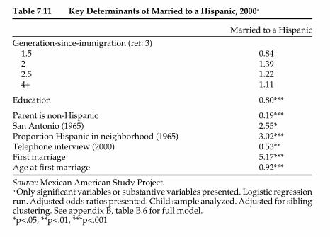
integrated into Mexican American families. More importantly, most ofthe population does not intermarry. Even if there are significant rates ofintermarriage, however, the progeny of such intermarriages will oftenassume a Mexican or Mexican American identity, as we will show inchapter 9. A related issue is the extent to which the children of such inter-marriages are identifiable as Mexicans. The point for this chapter, though,has merely been the extent of contact that Mexican origin persons havewith others.
Factors Affecting Intermarriage
We ran a logistic regression to examine which factors influence whetherrespondents married another Hispanic and present the results on table 7.11.Rather than regression coefficients, we present the more readily inter-pretable odds ratios for intermarriage. Like residential segregation, inter-marriage is not significantly related to generation-since-immigration.Instead, the chances of marrying another Hispanic are more stronglyrelated to the urban ecology of one’s neighborhood of upbringing. Sincethe odds ratios for urban area and Hispanic neighborhood are greaterthan 1, this indicates that San Antonians and those growing up in moreHispanic neighborhoods are more likely to marry other Hispanics. On theother hand, those interviewed by telephone (generally those who moved
Table 7.11 Key Determinants of Married to a Hispanic, 2000a
Married to a Hispanic
Generation-since-immigration (ref: 3)1.5 0.842 1.392.5 1.224+ 1.11
Education 0.80***
Parent is non-Hispanic 0.19***San Antonio (1965) 2.55*Proportion Hispanic in neighborhood (1965) 3.02***Telephone interview (2000) 0.53**First marriage 5.17***Age at first marriage 0.92***
Source: Mexican American Study Project.a Only significant variables or substantive variables presented. Logistic regressionrun. Adjusted odds ratios presented. Child sample analyzed. Adjusted for siblingclustering. See appendix B, table B.6 for full model.*p<.05, **p<.01, ***p<.001
Interethnic Relations 179
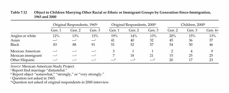
Table 7.12 Object to Children Marrying Other Racial or Ethnic or Immigrant Groups by Generation-Since-Immigration, 1965 and 2000
Original Respondents, 1965a Original Respondents, 2000b Children, 2000b
Gen. 1 Gen. 2 Gen. 3 Gen. 1 Gen. 2 Gen. 3 Gen. 2 Gen. 3 Gen. 4+Anglos or white 12% 13% 13% 19% 14% 13% 20% 15% 13%Asian —c —c —c 41 40 32 45 36 37Black 83 88 91 51 52 57 54 50 46
Mexican American —c —c —c 3 1 1 2 4 9Mexican immigrant —c —c —c 7 18 21 15 25 25Other Hispanic —c —c —c —d —d —d 20 17 23
Source: Mexican American Study Project.a Report find marriage “distasteful.”b Report object “somewhat,” “strongly,” or “very strongly.”c Question not asked in 1965.d Question not asked of original respondents in 2000 interview.
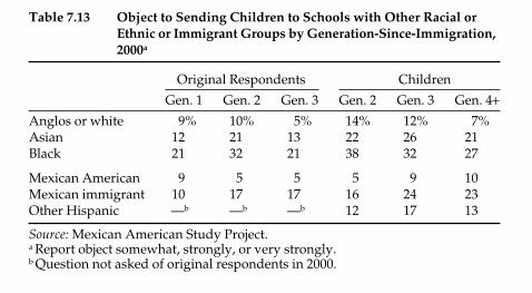
182 Generations of Exclusion
suggests that social distance between Mexican Americans and blacks belieany claim that racial attitudes have improved. On the other hand, theantiblack attitudes are still considerably greater than antiwhite attitudes,which hovered around the 12 to 19 percent range in 1965 and in 2000.Thus, any voiced opposition to marriage is very low for whites butremains considerable when it comes to blacks.
These figures also reveal the extent to which Mexican Americans havehistorically distanced themselves from African Americans. Althoughleading “whiteness” scholars have argued that European immigrants andtheir descendants—especially Jews, the Irish, and Italians—becameaccepted as white, mostly because they were able to distance themselvesfrom blacks and cope with their own low social status by seeing them-selves as hardworking and morally superior to the negative caricaturesof blacks.27 However, the same does not appear to have allowed MexicanAmericans to become white. In both 1965 and 2000, our data show thatMexican Americans created social boundaries from blacks while theywere closest to whites, both in intermarriage and in racial attitudes.
In 2000, we also asked about objection to marriages with Mexican immi-grants, U.S.-born Mexican Americans, other Hispanics, and Asians. Table7.12 shows almost no opposition to marriage with other MexicanAmericans, despite the surprising 9 percent of fourth-generation respon-dents. Opposition to marriage with Mexican immigrants was in mostcases greater than opposition to marriage with Anglos. Opposition tomarriage with blacks ranged from 46 to 54 percent, and opposition tomarriage with Asians was also large—between 36 and 45 percent.
We also asked in the 2000 questionnaire about opposition to attendingschools attended primarily by one or another of these groups. Table 7.13
Table 7.13 Object to Sending Children to Schools with Other Racial orEthnic or Immigrant Groups by Generation-Since-Immigration,2000a
Original Respondents Children
Gen. 1 Gen. 2 Gen. 3 Gen. 2 Gen. 3 Gen. 4+Anglos or white 9% 10% 5% 14% 12% 7%Asian 12 21 13 22 26 21Black 21 32 21 38 32 27
Mexican American 9 5 5 5 9 10Mexican immigrant 10 17 17 16 24 23Other Hispanic —b —b —b 12 17 13
Source: Mexican American Study Project.a Report object somewhat, strongly, or very strongly.b Question not asked of original respondents in 2000.

Culture and Language 193
Spanish and English are mixed—or, as some call it, “speaking Spanglish”or “code-switching”—may mark one as both Mexican and American or per-haps as neither, depending on the context. A speaker of Spanglish may beperceived as fluent in two languages, which marks them as both Americanand Mexican, or as unable to fully communicate in either, marking themas not fully American or Mexican. Alternatively, Spanglish speakers maybe fluent in one or both languages but code switch as a signal of theirMexican American ethnicity or to signal intimacy, informality, or a com-mon bond with listeners. On the other hand, the consequences may bequite negative. A study by Thomas Purnell, William Idsard, and John Baughfound that landlords consistently failed to return calls about inquiries frompotential renters who spoke in Chicano English but regularly returnedcalls from those who spoke standard English.33 For this, we asked respon-dents how often or whether they mixed Spanish and English in the samesentence.
Source: Mexican American Study Project.a Report spoke “mostly” or “only” English.b As reported by original respondents.
Generation-Since-Immigration
1
2
3
4+
Parents ofOriginalRespondentsb
6%
20%
Original Respondents
11%
31%
41% 62%
57%
17%
1965 2000
74%
82%
83%
2000
Children ofOriginalRespondents
Figure 8.1 Spoke English to Children by Generation-Since-Immigration,1965 and 2000a
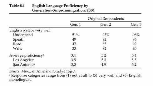
Culture and Language 189
English well or very well in 2000, as the first column of table 8.1 shows.By the second generation, more than 90 percent are. Thus, in the 1960s,the transition to English was almost complete for the children of immi-grants. By the third generation, 96 percent are able to understand or speakEnglish fluently, and more than 90 percent can read and write in English.The final three rows of table 8.1 summarize levels of English proficiencyacross generations-since-immigration, for the original respondents andseparately for Los Angeles and San Antonio. This scale is an average ofresponses from “not at all” (coded as 1) to “very well” (coded as 5) andEnglish monolinguals (coded as 6) to four questions regarding under-standing, speaking, reading, and writing the language. English abilityincreases sharply from immigrants to their children and then levels off inthe third generation for the original respondents. The generational pat-tern is similar for Los Angeles and San Antonio, though English fluencyis somewhat greater in Los Angeles. These results are only for the parentalgeneration, which was mostly raised in the 1930s, 1940s, and 1950s whenmany Mexican Americans had relatively little contact with Americaninstitutions, including schools.
For the child generation raised in the 1950s, 1960s, and 1970s, Englishproficiency is universal for the U.S.-born. All of the children completed the2000 interview in English. That is, 100 percent of the children respondentswere at least able to understand English well, which is not surprising asmost of the literature has shown.
Persistence of Spanish over Time
The important issue in the intergenerational transfer of linguistic abilityamong Mexican Americans, then, is the extent to which Spanish is
Table 8.1 English Language Proficiency by Generation-Since-Immigration, 2000
Original Respondents
Gen. 1 Gen. 2 Gen. 3
English well or very wellUnderstand 51% 93% 96%Speak 49 92 96Read 47 85 92Write 33 82 90
Average proficiencya 3.4 5.2 5.4Los Angelesa 3.5 5.3 5.5San Antonioa 3.0 4.9 5.2
Source: Mexican American Study Project.a Response categories range from (1) not at all to (5) very well and (6) Englishmonolingual.

190 Generations of Exclusion
retained. English is universally acquired, making it not an issue amongthe U.S.-born. If Spanish is retained, we can assume that MexicanAmericans are bilingual. If not, they are English monolingual. Table 8.2shows that among the original respondents or the parental generation, alarge number of the second and third generation understood and spokeSpanish. Three-quarters or more of the second and third generation couldunderstand or speak Spanish well or very well, though only a third (33 per-cent) of the third generation could read and about one-quarter (26 percent)could write at that level.
Spanish-language retention into the second generation of the child sam-ple seems to have remained nearly the same as it did for the second gen-eration among original respondents. Fully 89 percent understood Spanishwell or very well. However, the extent to which the third generationretained Spanish dropped considerably in comparison to original respon-dents of the same generation. For example, 82 percent of the third gener-ation among original respondents could understand Spanish, but only57 percent of the children could. As signs of further erosion, 46 percent ofthe fourth generation could understand Spanish, compared to 82 percentof their third-generation parents. In terms of speaking, reading, and writ-ing, less than half of third-generation parents passed them on to their chil-dren. It seems that while these parents had Spanish-language abilities, thehome language was more than likely to have been exclusively English.This suggests that the social context, at home and outside it, in which thethird generation was raised was more Spanish-speaking before the 1960s.Nevertheless, the fact that nearly half of today’s fourth generation adults
Table 8.2 Spanish Language Proficiency by Generation-Since-Immigration, 2000
Original Respondentsa Childrenb
Gen. 1 Gen. 2 Gen. 3 Gen. 2 Gen. 3 Gen. 4+Spanish well to very wellUnderstand 98% 89% 82% 89% 57% 46%Speak 98 87 75 79 40 36Read 91 42 33 43 19 11Write 89 39 26 36 11 7
Average proficiency 5.3 3.9 3.5 3.7 2.8 2.3Los Angeles 5.3 3.9 3.3 3.7 2.6 2.0San Antonio 5.2 4.1 3.9 3.7 3.2 3.1
Source: Mexican American Study Project.a Response categories range from (1) not at all to (5) very well and (6) Spanishmonolingual for original respondents.b Scale range from (1) not at all to (5) very well for children.
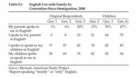
Culture and Language 191
understand Spanish defies the three-generation assimilation model andprobably far surpasses the experience of any other ethnic group.
The final three rows of table 8.2 summarize levels of proficiency acrossgenerations-since-immigration, for the entire sample and separately for LosAngeles and San Antonio. This scale is an average of responses from “not atall” (coded as 1) to “very well” (coded as 5) and Spanish monolingual (codedas 6) to four questions regarding understanding, speaking, reading, andwriting the language. Spanish ability sharply declines from nearly univer-sal fluency from immigrants to their children and then drops to a moderateamount in the third generation, at least for the original respondents. Thethird generation drop-off, though, is much stronger among their children’sgeneration, with continuing erosion into the fourth generation. AlthoughSpanish proficiency is the same for the second generation in the two urbanareas, the language is preserved to a greater extent among the third andfourth generation in San Antonio than in Los Angeles. Despite greater soci-etal openness to the use of foreign languages in the United States, Spanishis not being preserved as it used to be, in Los Angeles or San Antonio. Thedecline of Spanish use among the U.S.-born and its minimal use in LosAngeles contradicts the idea that bilingualism has a greater chance in a soci-ety with mass immigration from Mexico. On the other hand, greater Spanishloss is consistent with a hypothesis that social boundaries between MexicanAmericans and the mainstream have softened in the post–civil rights era.
Table 8.3 shows English-language use, when the respondents were chil-dren and when they had children, based on their recollection. If one looksfrom top to bottom in each column, table 8.3 shows that English usageclearly increases with each family generation, independent of generations
Table 8.3 English Use with Family by Generation-Since-Immigration, 2000
Original Respondents Children
Gen. 1 Gen. 2 Gen. 3 Gen. 2 Gen. 3 Gen. 4+My parents spoke to 1% 6% 20% 13% 55% 67%me in Englisha
I spoke to my parents 0 8 23 21 64 75in Englisha
I spoke or speak to my 17 57 62 74 82 83children in Englisha
My children spoke 30 69 74 82 92 94or speak to me in Englisha
Source: Mexican American Study Project.a Report speaking “mostly” or “only” English.
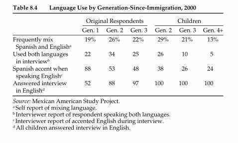
194 Generations of Exclusion
The first row of table 8.4 shows that 19 to 26 percent of original respon-dents in the first to third generations report that they sometimes or fre-quently mix Spanish and English. The second generation was the mostlikely to code-switch, perhaps reflecting their fluency and greater expo-sure to both languages. Interestingly, reported mixing of both languagesremained high for second- and third-generation children. This may reflecta greater need to communicate in Spanish to a growing immigrant pop-ulation in the 1990s, accompanied by a growing inability among later gen-eration Mexican Americans to speak fluent Spanish. However, there is asignificant drop in Spanglish from the third-generation original respon-dents to the fourth-generation children. By the fourth generation, only13 percent of respondents continued to mix the two languages. By thatpoint, most apparently did not know enough Spanish to mix with English.
The second row of table 8.4 reports, according to the interviewer,whether Spanish and English was actually mixed during the interview.Again, the second generation of the original respondents used mixedSpanish and English the most. However, among the children, self-reportedSpanglish use and that reported by interviewers differed by generation.Interestingly, interviewers reported use of both languages among 5 to10 percent of the third- and fourth-generation children, versus 26 percentof the second-generation children and 34 and 25 percent of the second-and third-generation original respondents. This is consistent with thedecline in Spanish among third- and fourth-generation children.
On the other hand, the third row shows that interviewers reportedthat 38 percent of the second generation and 24 to 26 percent of the thirdand the fourth generation in the child sample continued to have Spanish
Table 8.4 Language Use by Generation-Since-Immigration, 2000
Original Respondents Children
Gen. 1 Gen. 2 Gen. 3 Gen. 2 Gen. 3 Gen. 4+Frequently mix 19% 26% 22% 29% 21% 13%Spanish and Englisha
Used both languages 22 34 25 26 10 5in interviewb
Spanish accent when 88 53 48 38 26 24speaking Englishc
Answered interview 52 88 97 100 100 100in Englishd
Source: Mexican American Study Project.a Self report of mixing language.b Interviewer report of respondent speaking both languages.c Interviewer report of accented English during interview.d All children answered interview in English.

Culture and Language 195
accents when speaking English (as perceived by the interviewer). This com-pares to accented English pronunciation among fully half of the second-and third-generation original respondents. The last row in table 8.4 showsthe percentage of respondents interviewed in English. On the one hand, allof the children answered the English questionnaire. On the other, complet-ing the interview among the original respondents varied by generationalstatus—half of first generation original respondents completed our inter-view in Spanish, but only a handful among the second and third genera-tion did so.
Factors Affecting Spanish Proficiency
To examine which factors affect Spanish proficiency, we conducted a regres-sion analysis. We ran a linear regression, because this is a continuousvariable, and present unstandardized coefficients for significant inde-pendent variables in table 8.5. Generational status is a significant predic-tor of Spanish-language proficiency. There is a constant decline across thefive generations or subgenerations in Spanish proficiency, suggesting slowbut linear language shift. Each generation is less proficient in Spanishthan the generation or half-generation before, all at a statistically signifi-cant level when compared to the third generation. This mirrors the resultsof the bivariate analysis: linguistic assimilation occurs independently ofall the variables in the models.
Table 8.5 Key Determinants of Spanish Proficiency, 2000a
Spanish Proficiencyb
Generation-since-immigration (ref: 3)1.5 0.73***2 0.37**2.5 0.32***4+ −0.20*
Education 0.09***
Mother’s education −0.02*Parent spoke Spanish to child 0.88***Parent is non-Hispanic −0.30*San Antonio (1965) 0.36***Female 0.13*
Source: Mexican American Study Project.a Only significant variables or substantive variables presented. Linear regressionrun. Unstandardized coefficients presented. Child sample analyzed. Adjusted forsibling clustering. See appendix B, table B.7 for full model.b Based on average proficiency reported on table 8.2.*p<.05, **p<.01, ***p<.001
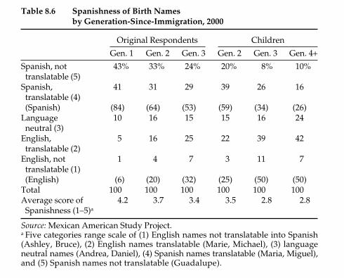
Culture and Language 197
name will establish a strong ethnic identity in the child to the belief that anon-ethnic name will improve a child’s acceptance in the host society.Although parents may choose from a wide variety of names, their choicesare in reality shaped by social and cultural influences. Finally, birth nameshave obvious long-term consequences: as labels, they influence the social-ization of children and contribute to the development of personal identities.
In our 2000 survey, we asked both the original respondent and chil-dren samples what their name was on their birth certificate. With thisinformation, we coded all of the first names into five categories that seekto capture a continuum of English to Spanish names. The first categoryrepresents the most English names and the last represents the most Spanish.Specifically, category 1 refers to English names that are not translatable intoSpanish (such as Ashley and Bruce), category 2 includes English namesthat are translatable (Marie, Michael), category 3 to language neutral names(Daniel, Andrea), category 4 to translatable Spanish names (Maria, Miguel),and category 5 to not translatable Spanish names (Guadalupe). Thesenames were coded 1 to 5 by a panel of bilingual persons.36
The first row of table 8.6 shows that, among the original respondents,fully 43 percent of immigrants were given untranslatable Spanish names,
Table 8.6 Spanishness of Birth Names by Generation-Since-Immigration, 2000
Original Respondents Children
Gen. 1 Gen. 2 Gen. 3 Gen. 2 Gen. 3 Gen. 4+Spanish, not 43% 33% 24% 20% 8% 10%translatable (5)
Spanish, 41 31 29 39 26 16translatable (4)(Spanish) (84) (64) (53) (59) (34) (26)
Language 10 16 15 15 16 24neutral (3)
English, 5 16 25 22 39 42translatable (2)
English, not 1 4 7 3 11 7translatable (1)(English) (6) (20) (32) (25) (50) (50)
Total 100 100 100 100 100 100Average score of 4.2 3.7 3.4 3.5 2.8 2.8
Spanishness (1–5)a
Source: Mexican American Study Project.a Five categories range scale of (1) English names not translatable into Spanish(Ashley, Bruce), (2) English names translatable (Marie, Michael), (3) languageneutral names (Andrea, Daniel), (4) Spanish names translatable (Maria, Miguel),and (5) Spanish names not translatable (Guadalupe).
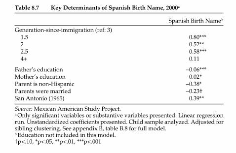
Culture and Language 199
non-Hispanic parent meant that one was less likely to be given a Spanishname. San Antonians are clearly more likely to have Spanish names inde-pendent of all other effects.
Religion and ReligiosityAside from language, perhaps the cultural trait most associated withMexican Americans has been Catholicism, which also serves as a markerdistinguishing Mexican Americans from most other ethnic groups. Manyof the poorest and most despised Europeans, particularly the Irish, Italians,and Poles, were strongly Catholic. However, their children and grandchil-dren seem to have moved to a more secular mindset.37 Whether MexicanAmericans similarly choose to “adopt American ideals of individualism”and a quest for prosperity in place of “religious ideals of community,” as arecent New York Times article put it, is not clear.38 The data on such a trendis not clear for any group, especially since the U.S. Census has not collecteddata on religion since 1950. Several national surveys of religion, though,were taken between 1991 and 2004. Catholics have comprised about one-quarter (23 to 26 percent depending on the estimate and the year) of allAmericans, and about one-third of American Catholics are Hispanic.39
Finke and Stark stress the vitality and growth of Catholicism throughoutAmerican history.40 However, they raise the concern that Catholicism maybecome like other mainline religions with a declining membership base.They note that Hispanic immigration has not helped Catholic expansion asmuch as many have expected because many Hispanic immigrants have
Table 8.7 Key Determinants of Spanish Birth Name, 2000a
Spanish Birth Nameb
Generation-since-immigration (ref: 3)1.5 0.80***2 0.52**2.5 0.58***4+ 0.11
Father’s education −0.06***Mother’s education −0.02*Parent is non-Hispanic −0.38*Parents were married −0.23†San Antonio (1965) 0.39**
Source: Mexican American Study Project.a Only significant variables or substantive variables presented. Linear regressionrun. Unstandardized coefficients presented. Child sample analyzed. Adjusted forsibling clustering. See appendix B, table B.8 for full model.b Education not included in this model.†p<.10, *p<.05, **p<.01, ***p<.001
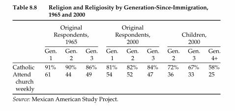
200 Generations of Exclusion
converted to evangelical religions and their children are even more likelyto not be Catholic. Noting widely inconsistent estimates of the religiousidentities of Hispanics among national surveys, Paul Perl, Jennifer Greely,and Mark Gray find several methodological problems with them and arguethat the most reliable estimates reveal that about 70 percent of Hispanicsare Catholics and another 20 percent are Protestant.41 Based on these cross-sectional surveys, they further estimate a downward shift in the proportionof U.S.-born Catholic Hispanics from 74 percent in the first to about 50 per-cent in the third generation. Espinosa and colleagues find a smaller declinefrom 74 to 62 percent across the three generations.42 Religion is also relatedto politics, as 63 percent of Hispanic Protestants voted for Bush, comparedto only 31 percent of Hispanic Catholics.43
Our data reveal a similar pattern across generations-since-immigrationbut also show that historical changes may be even more important. Amongoriginal respondents in 1965, about 90 percent of Mexican Americans wereCatholic, with 91 percent of immigrants being Catholic and only slightreligious assimilation in succeeding generations. By 2000, an additional8 to 10 percent of the original respondents were no longer Catholic inthe first and second generation, while there was relatively little declinefor the third generation, as table 8.8 demonstrates.
Many fewer children, though, were Catholic. Generational differenceshad also become large, suggesting the emergence of religious accultura-tion. Among the second generation, only 72 percent were Catholic, versus90 percent of second-generation original respondents were when theywere young. By the fourth generation, only 58 percent were Catholic,though they were generally raised in households where 86 percent of theiroriginal-respondent parents were Catholic. Additionally, from 1965 to2000, there is a sharpening of differences by generation-since-immigrationbetween original respondents and their children for the entire MexicanAmerican population. These results would have been startling to the inves-
Table 8.8 Religion and Religiosity by Generation-Since-Immigration,1965 and 2000
Original OriginalRespondents, Respondents, Children,
1965 2000 2000
Gen. Gen. Gen. Gen. Gen. Gen. Gen. Gen. Gen.1 2 3 1 2 3 2 3 4+
Catholic 91% 90% 86% 81% 82% 84% 72% 67% 58%Attend 61 44 49 54 52 47 36 33 25churchweekly
Source: Mexican American Study Project.
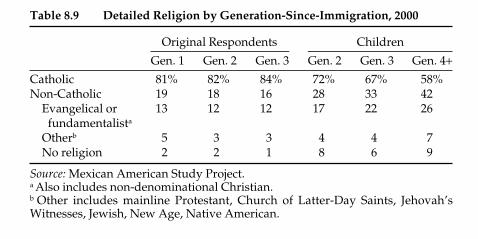
Culture and Language 201
tigators of the original project, who were particularly interested in therole of the Catholic Church. Grebler, Moore, and Guzmán interviewedparish priests and reported that “no pastor interviewed seems to takeProtestant proselytizing seriously.”44 The same religious shift among thegeneral American (and Latin American) Catholic and Protestant religionsto evangelicalism might have been similarly surprising, however.
To be sure, some Catholics are Catholic in name only. They were bap-tized as Catholics and may continue to have a Catholic identity, but rarelypractice their religion. More generally, however, Hispanics are believedto be religious as well as predominantly Catholic. Table 8.8 demonstratesthe extent to which this is true by measuring religiosity and, more specif-ically, the proportion who attended religious services at least once perweek, regardless of their religion. Like the question on religious identity,a question on religiosity was asked in both the 1965 and the 2000 surveys.
Whereas changes in church attendance from 1965 to 2000 were mixed fororiginal respondents, table 8.8 also demonstrates that religiosity droppedacross the board from the parents to the children’s generation. Only 25 to36 percent of children among those who declared they belonged to a reli-gion were regular church-goers, versus 44 to 61 percent of their parents.Also, generation-since-immigration differences sharpened for children,which mirrors the intergenerational findings for Catholic affiliation. Forexample, where 36 percent of the second generation attended churchweekly, only 25 percent of the fourth generation did. Among the originalrespondents, the percent who attended church weekly dropped from thefirst generation (61 percent) to the second generation (44 percent), butthen it leveled off in the third generation (49 percent).
Table 8.9 shows that the decline in the number of Catholics since the1960s and across generations was due mostly to the countertrend in thegrowing proportion that joined evangelical or fundamentalist Christian
Table 8.9 Detailed Religion by Generation-Since-Immigration, 2000
Original Respondents Children
Gen. 1 Gen. 2 Gen. 3 Gen. 2 Gen. 3 Gen. 4+Catholic 81% 82% 84% 72% 67% 58%Non-Catholic 19 18 16 28 33 42
Evangelical or 13 12 12 17 22 26fundamentalista
Otherb 5 3 3 4 4 7No religion 2 2 1 8 6 9
Source: Mexican American Study Project.a Also includes non-denominational Christian.b Other includes mainline Protestant, Church of Latter-Day Saints, Jehovah’sWitnesses, Jewish, New Age, Native American.
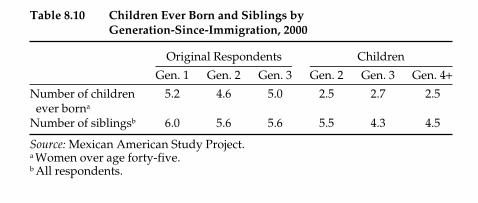
Culture and Language 203
Because our sample size is relatively small, especially when the agerange was restricted, we were unable to analyze fertility rates in detail.Instead, we examined the number of children ever born in table 8.10, asreported by our female respondents forty-five years old and older, whenthey had completed virtually all of their childbearing.51 We found few gen-erational differences in the number of children ever born among eitheroriginal respondents or children. Immigrant fertility was a little higherthan for the second generation among the original respondents, whichin turn was lower than it was for the third generation. Among children,fertility was cut by about half of their parents’, reflecting the overall nationaltrend from baby boom to baby bust. Moreover, there were no significantdifferences by generation. The number of children ever born for motherswho had completed their fertility was 2.5 or 2.7 for all the U.S.-born ofthe children’s generation, which includes second, third, and fourthgeneration-since-immigration and is exactly the same as that for forty-to forty-four-year-old second- and third-generation Mexican Americansbased on the 1998 to 2002 Current Population Survey.52
We also asked respondents to report the number of brothers and sis-ters they had, including any who had died. The second row of table 8.10shows the number of siblings for our respondents, which reflects theirparents’ fertility experiences, combined with results in the first row, approx-imates the experiences of three family generations. Fertility declined pre-cipitously across the generations. The original respondents averages aboutfive children, compared to about two and one-half for their children. Thenumber of siblings also reveals relatively high fertility for the originalrespondents and their parents.53 Results for number of children amongthe original respondents and the siblings among the children were con-sistent and reveal greater fertility for the third generation among originalrespondents. For generation-since-immigration, sibling results were likethose for number of children. In sum, the findings again reveal somewhatgreater fertility for immigrants and declining fertility from grandparentsto parents to children.
Table 8.10 Children Ever Born and Siblings by Generation-Since-Immigration, 2000
Original Respondents Children
Gen. 1 Gen. 2 Gen. 3 Gen. 2 Gen. 3 Gen. 4+Number of children 5.2 4.6 5.0 2.5 2.7 2.5ever borna
Number of siblingsb 6.0 5.6 5.6 5.5 4.3 4.5
Source: Mexican American Study Project.a Women over age forty-five.b All respondents.
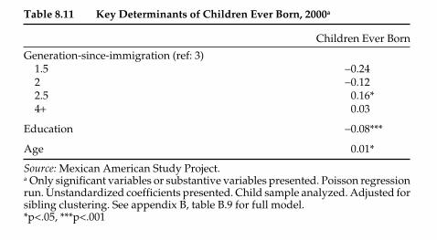
204 Generations of Exclusion
To examine which factors affect the number of children ever born, weconducted a regression analysis, using a poisson model because this isan ordinal variable. We present unstandardized coefficients for significantindependent variables in table 8.11. Generational differences in fertilitywere not significant with the exception of generation 2.5 having signifi-cantly more children than the third generation. The one strong predictorof fertility is education—with more educated women having fewer chil-dren. Age was also significant in that older women had more children,which is expected given that childbearing decreased sharply from the1970s to the 1990s.54
Family ValuesPro-natalist values are commonly thought to operate in tandem with tradi-tional family roles. Early research blamed rigid and authoritarian familiesfor the slow socioeconomic progress of Mexicans and Mexican Americans.55
In particular, male dominance over the family and rigid gender roles werethought to prevent positive personality development and hinder individualachievement and mobility, though they were believed to provide emotionaland economic security. In his review of these studies, Alfredo Mirandé didnot so much argue that this portrait of Chicano familism was inaccurate asthat it had features that have served Mexican Americans well, in large partby providing refuge from oppressive American economic and culturalcolonialism.56 Moreover, such a model could not be generalized to the entireMexican American population, because Mexican familism had beenlargely eroded because of acculturation and urbanization.57 On the otherhand, Mirandé argued that the traditional family and familistic values
Table 8.11 Key Determinants of Children Ever Born, 2000a
Children Ever Born
Generation-since-immigration (ref: 3)1.5 −0.242 −0.122.5 0.16*4+ 0.03
Education −0.08***
Age 0.01*
Source: Mexican American Study Project.a Only significant variables or substantive variables presented. Poisson regressionrun. Unstandardized coefficients presented. Child sample analyzed. Adjusted forsibling clustering. See appendix B, table B.9 for full model.*p<.05, ***p<.001
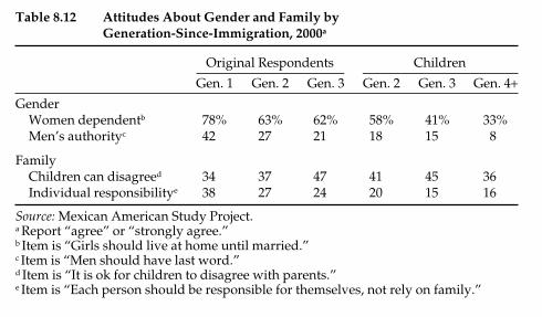
Culture and Language 205
have been largely maintained into later generations because of proximityto Mexico and because they have served to shield children from an oppres-sive social world.
This celebration of patriarchal values and familism among MexicanAmericans was subsequently criticized by Chicana feminists. MaxineBaca Zinn and Lea Ybarra were among the first to take Mirandé to taskbecause he had not adequately considered the structural factors affectingMexican American families or the diversity among them.58 Both argued,in fact, that Mexican American families were, in some circumstances,egalitarian. A second generation of Chicana feminists added further com-plexity to the critique. For example, Patricia Zavella argued that Chicanofamilies are diverse and frequently patriarchal, but so are Anglo fami-lies.59 Moreover, she heeded scholars to separate ideology from reality:even though husbands and wives will frequently voice patriarchal views,the reality is by necessity more complex and sometimes egalitarian. Debatesabout the extent of familism and traditional values continue in more recentresearch.60
To investigate the extent of agreement with traditional family and gen-der attitudes and whether these persist across time and over generations,we asked respondents whether they agreed that girls should live at home,men should have the last word, whether it is acceptable for children todisagree with parents, and whether individuals should rely on their fam-ilies. These results are presented in table 8.12. The questions about appro-priate gender roles—whether girls should live at home and men shouldhave the last word—show a familiar pattern: immigrants and originalrespondents hold the most traditional gender attitudes. Traditional gender
Table 8.12 Attitudes About Gender and Family by Generation-Since-Immigration, 2000a
Original Respondents Children
Gen. 1 Gen. 2 Gen. 3 Gen. 2 Gen. 3 Gen. 4+Gender
Women dependentb 78% 63% 62% 58% 41% 33%Men’s authorityc 42 27 21 18 15 8
FamilyChildren can disagreed 34 37 47 41 45 36Individual responsibilitye 38 27 24 20 15 16
Source: Mexican American Study Project.a Report “agree” or “strongly agree.”b Item is “Girls should live at home until married.”c Item is “Men should have last word.”d Item is “It is ok for children to disagree with parents.”e Item is “Each person should be responsible for themselves, not rely on family.”

206 Generations of Exclusion
attitudes lessen with generation-since-immigration and from parents tothe children61
On the other hand, the results for the other two questions (rows threeand four) were unexpected. The third row refers to individualism versusfamilism, which Huntington, like many before him, believe representsa cultural divide that explains differences in economic success betweenMexican Americans and Anglos.62 Mexicans, these scholars argue, are toofamily oriented and not individualistic enough, which impedes them frommoving up and out of the working class. However, the results show thatimmigrants are generally the most individualistic and that the parental gen-eration has the highest proportions of persons believing that they shouldbe responsible for themselves (row 4). Apparently, later generations preferto rely on their families. Thus, these findings show that belief in the valueof individualism is stronger for immigrants and the more ethnic parentalgeneration, which is consistent with de la Garza and his colleagues.63 Theindividualism of immigrants makes sense if we consider that they weremotivated enough to have left their own communities in search of workopportunities hundreds of miles away in a very culturally distinct place.
MusicFinally, we sought to measure the extent to which ethnic popular culturepersists across generations, especially given the enduring persistence ofU.S.-based Chicano culture and the diffusion of Spanish media through-out much of the Southwest.64 We asked respondents to name theirfavorite genre of music in an open-ended question. We coded responsesinto categories consisting of more than thirty genres including rock androll, rancheras, Tex-Mex, big band, and jazz. We then created three gen-eral categories to capture a continuum of ethnic preferences, which wepresent in table 8.13. The American–black music category includes suchgenres as rock, swing, country, soul, and American-English in general.The Mexican category includes banda, cumbia, ranchera, or Mexican-Spanish in general. We also created an intermediate category to capture
Table 8.13 Favorite Music by Generation-Since-Immigration, 2000
Original Respondents Children
Gen. 1 Gen. 2 Gen. 3 Gen. 2 Gen. 3 Gen. 4+American, black 20% 37% 46% 55% 59% 65%Chicano (oldies, 3 15 23 27 29 25Tex-Mex, Latin)
Mexican 74 44 29 15 9 9No preference 3 4 1 3 3 0
Source: Mexican American Study Project.
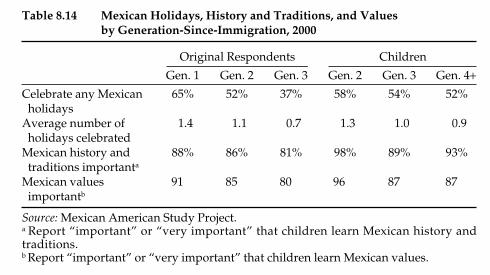
208 Generations of Exclusion
attend such a celebration whereas the generation mostly in their fortiesand fifties may seek to instill ethnic pride in their children by celebrat-ing an ethnic holiday. Also, these were self-reports based on a generalquestion about whether respondents celebrate Mexican holidays, whichthey then named.
Perceptions of discrimination and identity differed greatly betweenMexican Americans and European ethnics in later generations, but theextent to which they celebrated holidays differed to a lesser extent. Fully27 percent of European ethnics participated in ethnic festivals or cele-brations in the Albany study by Richard Alba.67 Participation in ethnicholidays, though, requires little knowledge of or investment in one’s eth-nicity. Observing ethnic celebrations may be similar for both groups, butethnicity is a different experience altogether for Mexican Americans. Forthe descendants of Europeans, ethnicity is largely symbolic. For MexicanAmericans, it is much more bound up with other life experiences, as thisand the following chapters show.
The last two rows of table 8.14 show that at least 80 percent of MexicanAmericans in all generations believe that children should learn aboutMexican history, tradition, and values. Mexican history and values seemto be cherished among the vast majority of even those Mexican Americansmost removed from the immigration experience, at the point that theywould like their children to learn about them. These findings, like thoseshowing significant ethnic holiday observance, demonstrate that fourth-generation Mexican Americans at least hold the symbolic ethnicity of later-generation European Americans. However, based on an abundance ofother evidence in this book, there can be no doubt that there is more than
Table 8.14 Mexican Holidays, History and Traditions, and Values by Generation-Since-Immigration, 2000
Original Respondents Children
Gen. 1 Gen. 2 Gen. 3 Gen. 2 Gen. 3 Gen. 4+Celebrate any Mexican 65% 52% 37% 58% 54% 52%holidays
Average number of 1.4 1.1 0.7 1.3 1.0 0.9holidays celebrated
Mexican history and 88% 86% 81% 98% 89% 93%traditions importanta
Mexican values 91 85 80 96 87 87importantb
Source: Mexican American Study Project.a Report “important” or “very important” that children learn Mexican history and traditions.b Report “important” or “very important” that children learn Mexican values.
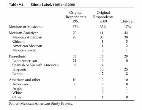
and business endorsed categories that bring together the growing diversityamong persons of Spanish-speaking origin, though they may also continueto serve as euphemisms for Mexican.
In the 2000 survey, respondents were asked: “People have differentways of thinking about their ethnic background or origins. What aboutyou? How do you think of yourself: What do you consider your ethnicbackground to be?”
Unlike the question in the 1965 survey, ours is strictly open-ended.That is, we did not provide any response categories but let respondentsgive their own answers.13 The open-ended question in 2000 thus allowsfor more categories of ethnic identification than did the 1965 item, whichwas only partially open-ended.
The second column of table 9.1 shows that a combined 74 percent ofthe original respondents preferred one of the categories of Mexican (orMexicano) and Mexican American in 2000. The original respondents in2000 are half as likely to use pan-ethnic terms and twice as likely to useMexican American regardless of their preferences thirty-five years ago.Because the distribution of the 1965 and the 2000 respondents differ greatly,we examine how the 1965 responses changed by 2000 below.
Column three of table 9.1 indicates that the proportion of children iden-tifying as Mexican or Mexicano is less than half (17 percent) that of the
Ethnic Identity 215
Table 9.1 Ethnic Label, 1965 and 2000
Original OriginalRespondents Respondents
1965 2000 Children
Mexican or Mexicano 37% 33% 17%
Mexican American 20 41 44Mexican American 20 39 38Chicano 1 3American Mexican 1 2Mexican mixed 0 1
Pan-ethnic 33 16 29Latin American 24 0 0Spanish or Spanish American 9 4 1Hispanic 10 25Latino 2 2
American and other 10 10 10American 8 9 8Anglo 0 1White 0 1Other 2 1 0
Source: Mexican American Study Project.

included Mexicano, Mexicano-Americano, Latino, and Hispano. We sus-pect that the purpose of the Spanish question was to observe whetherone’s preferred ethnic label in a Spanish-language context might differfrom an English one. Table 9.2 compares the responses of those respond-ing to the English interview with the Spanish one. Among those answer-ing the English questionnaire, fully 18 percent of those choosing any termchose Latino and another 2 percent chose Hispano. This also reveals thatmost Mexican Americans understood Spanish well enough to haveanswered the question. Moreover, the second column of table 9.2 alsoshows that for those answering the Spanish questionnaire, in which thesame categories were given, 14 percent chose Latino and 1 percentHispano, though the question was not asked of most 1965 respondentsresponding in Spanish for reasons unknown to us.
To consider the issue of assimilation being so advanced that some ofMexican-origin may no longer identify as such, we examined the responsesof children whose primary ethnic identity was American, Anglo, white,or other. This is an important issue to explore because it addresses amethodological problem, raised by several researchers,15 that assimilatedMexican Americans might not identity as such and therefore be missedin analyses of ethnic and generational change. As already noted, we foundthat the large majority of children had identified as Mexican, MexicanAmerican, or Hispanic (which we refer to as a Hispanic identifier) at somepoint in the survey. Table 9.3 shows that of eighty-five persons whoseprimary identity is white, American, or other, forty-four also chose aHispanic identifier as a second ethnic identifier. Among those who did
Ethnic Identity 217
Table 9.2 Second Ethnic Label Question by Language of Interview, 1965a
Original Respondents
English SpanishQuestionnaire Questionnaire All
Mexicano 45% 65% 49%Mexico Americano 20 15 19Latino 18 14 17Hispano 2 1 1Tejano 2 1 1Americano 7 2 6Other 6 2 6Total 100 100 100
Number of valid responses 637 172 809Number missing responses 93 291 384
Source: Mexican American Study Project.a Asked in Spanish using different response categories in both English andSpanish questionnaires.
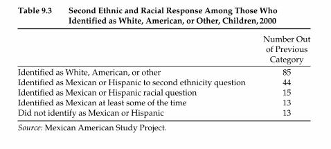
not, fifteen chose a Hispanic identifier as a racial identifier. Among theremaining respondents, thirteen reported that they think of themselvesas Mexicans at least some of the time. The last thirteen respondents reportno affinity with being Mexican or Hispanic in our survey. They represent,however, less than 2 percent of the entire sample. Thus, there is a poten-tially small degree of opting-out of the Mexican or Hispanic category. Ourevidence shows that this amount may be minimized, depending on theethnic questions in the survey, though it may remain a small problem.With our longitudinal study and intergenerational methodology, webelieve that we have nearly eliminated this problem.
Ethnic Identity by Urban Area
The use of particular ethnic terms largely depends on the local context, astable 9.4 shows. In Los Angeles in 1965, nearly half of the original respon-dents identified as Mexican (45 percent) and more than a quarter (26 per-cent) identified as Mexican American. This contrasts sharply with SanAntonio, where fully 59 percent identified as Latin American and only7 percent identified as Mexican American and 21 percent as Mexican,which is further evidence of the greater racial stigma of the word Mexicanin San Antonio. On the other hand, Spanish or Spanish American was usedby 10 percent in Los Angeles versus 6 percent in San Antonio, but this palesin comparison to the much greater use of the pan-ethnic Latin Americanused by 59 percent of San Antonians in 1965. Twelve percent in Los Angelesbut only 6 percent in San Antonio identified as American or other.
By 2000, the distribution of the preferred terms had somewhat convergedbetween the two cities, though the original respondents in San Antoniocontinued to prefer pan-ethnic terms, just as Angelenos had a greaterpreference for Mexican American. In 2000, fully 21 percent of the San
218 Generations of Exclusion
Table 9.3 Second Ethnic and Racial Response Among Those WhoIdentified as White, American, or Other, Children, 2000
Number Outof PreviousCategory
Identified as White, American, or other 85Identified as Mexican or Hispanic to second ethnicity question 44Identified as Mexican or Hispanic racial question 15Identified as Mexican at least some of the time 13Did not identify as Mexican or Hispanic 13
Source: Mexican American Study Project.
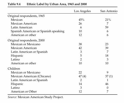
Antonio respondents interviewed in 1965 used Hispanic or Latino and only7 percent continued to prefer Latin American or Spanish. For their children,a similar pattern emerges except that fully 46 percent of San Antonians pre-ferred to be called Hispanic, which is nearly equal to the percentage whochoose the combined Mexican (9 percent) and Mexican American (37 per-cent) categories. In Los Angeles, only 19 percent chose a pan-ethnic term,and a full 69 preferred Mexican or Mexican American. These city differencessuggest that Mexican, or its derivative Mexican American, continue to bestigmatized in Texas, making it easier to identify as Hispanic.
We also show, in parentheses, the proportion of the children who preferthe term Chicano, which we put under the category Mexican Americanbut which has special significance as a term of political affirmation for somein that generation. Four percent used the term in Los Angeles comparedto only 1 percent in San Antonio, which is not surprising given apparentlymore intense ethnic politics in Los Angeles.16 Answers to further open-ended questions showed that many more of the children, especially in LosAngeles, occasionally think of themselves as Chicano though they mightprefer one of the more standard categories. They reported that the occa-sions in which they thought of themselves as Chicano were generally in
Ethnic Identity 219
Table 9.4 Ethnic Label by Urban Area, 1965 and 2000
Los Angeles San Antonio
Original respondents, 1965Mexican 45% 21%Mexican American 26 7Latin American 6 59Spanish American or Spanish speaking 10 6American or other 12 6
Original respondents, 2000Mexican or Mexicano 38 23Mexican American 42 39Latin American or Spanish 3 7Hispanic 5 18Latino 2 3American or other 10 10
ChildrenMexican or Mexicano 22 9Mexican American (Chicano) 47 (4) 37 (1)Latin American or Spanish 2 1Hispanic 14 46Latino 3 0American or Other 12 7
Source: Mexican American Study Project.

Table 9.5 Ethnic Label by Generation-Since-Immigration, 1965 and 2000
Original Respondents, 1965 Original Respondents, 2000 Children
Gen. 1 Gen. 2 Gen. 3 Gen. 1 Gen. 2 Gen. 3 Gen. 2 Gen. 3 Gen. 4+Mexican or Mexicano 56% 30% 27% 67% 25% 19% 28% 15% 10%Mexican American 21 26 10 15 51 43 43 43 44Pan-ethnica 20 31 44 11 14 26 25 30 33American or other 4 12 19 7 10 13 5 12 12
Source: Mexican American Study Project.a Pan-ethnic labels primarily Latin American and Spanish in 1965; primarily Hispanic and Latino in 2000.

the language effect is net of generation, thus not attributable simply to thechildren of immigrants being more or less likely to have these identities.We also expect that parent’s ethnicity should affect the children’s identi-fication. We find that children who have a non-Hispanic parent are morelikely to identify as American or other.25
The results in table 9.6 also show that persons raised in more Hispanicneighborhoods are more likely to identify as American or other. Theproportion Hispanic in a neighborhood refers to the neighborhood context in which the respondents were raised (based on 1970 censusdata for the census tract in which their parents were interviewed andwhere they resided in 1965). Because this finding is counterintuitive,we examined alternative models to learn what might be driving thiseffect. We get the effect in the multivariate analysis, but not when weexamine the effect of proportion Hispanic with no other variables in theanalysis. Moreover, we find it primarily with the Los Angeles sample(analysis not shown). This finding may be the result of U.S.-bornMexican Americans making quasi-ethnic distinctions by identifyingthemselves as American in distinction to immigrants, especially recentarrivals, in neighborhoods where there are few persons of any otherethnicity. The effect may be particularly strong in Los Angeles becausethe proportion of recent immigrants there is clearly greater than in SanAntonio.
224 Generations of Exclusion
Table 9.6 Key Determinants of Ethnic Label, 2000a
American orMexican Other
Generation-since-immigration (ref: 3)1.5 3.54** 0.612 1.01 0.542.5 0.88 0.604+ 0.76 1.24
Education 0.99 1.08
Parent spoke Spanish to child 2.65*** 0.36*Parent is non-Hispanic 2.27*San Antonio (1965) 0.27***Proportion Hispanic in neighborhood (1965) 2.66*Age 1.08**
Source: Mexican American Study Project.a Only significant variables or substantive variables presented. Logistic regressionrun. Compared to all other ethnic identities. Adjusted odds ratios presented.Child sample analyzed. Adjusted for sibling clustering. See appendix B, tablesB.10 and B.11 for full model.*p<.05, **p<.01, ***p<.001
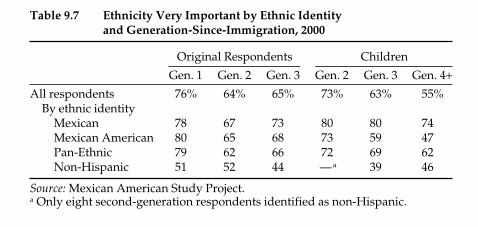
In addition, we find that San Antonio residents are less likely to use theMexican category than Angelenos, independent of all other effects in themodel. This might be due, in part, to the increased immigration in LosAngeles encouraging an identity as Mexican overall, though again, MexicanAmericans may be more likely to identify as American in those neighbor-hoods where there are few non-Mexicans. Among the respondent’s indi-vidual characteristics, only age affected ethnic identity. Older persons aremore likely to identify as American than any other identity. This probablyreflects the fact that the younger respondents came of age in the politicallyturbulent period of the late 1960s and early 1970s.
Salience of Ethnicity
That persons prefer to identify with a particular category may not reflecthow important ethnic identity is for them. Thus, we asked respondentsabout the salience or importance of their ethnic choice. Table 9.7 reportson those who claimed that their ethnic background was very importantto them, by generational status. The results indicate that ethnic identity wasmost salient for the first generation, at 76 percent. The second and thirdgeneration original respondents gave it somewhat less importance thanfirst generation but did not differ in the importance they gave to theirethnicity. Among the children, the importance of their ethnicity steadilydecreased by generation, from 73 to 55 percent. Next, we examine impor-tance by the four ethnic identity categories. For those identifying asMexican, ethnicity remained very important across all generations. As weshowed previously in table 9.5, the proportion identifying as Mexicandecreased in succeeding generations. It may be that the smaller groupthat continues to identify as Mexican in later generations does so becausethe ethnic category has significant meaning to them. More than half inalmost every category claim that their ethnicity is very important to them,
Ethnic Identity 225
Table 9.7 Ethnicity Very Important by Ethnic Identity and Generation-Since-Immigration, 2000
Original Respondents Children
Gen. 1 Gen. 2 Gen. 3 Gen. 2 Gen. 3 Gen. 4+All respondents 76% 64% 65% 73% 63% 55%
By ethnic identityMexican 78 67 73 80 80 74Mexican American 80 65 68 73 59 47Pan-Ethnic 79 62 66 72 69 62Non-Hispanic 51 52 44 —a 39 46
Source: Mexican American Study Project.a Only eight second-generation respondents identified as non-Hispanic.
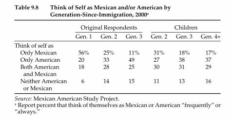
the third-generation respondents and 37 percent of their fourth-generationchildren. Thus, table 9.8 also provides evidence of ethnic resurgence. Fromthe third generation parents to their fourth generation children, there is aslight increase in the proportion feeling Mexican and a noticeable decreasein the proportion thinking of themselves as American. Of course, “frequentlythink” may mean different things to different people. Thus, one mayinterpret this table as showing a drop in the sense of feeling only Mexican,an increase in the sense of feeling American, but at the same time that 25to 31 percent frequently think of themselves as both, across generations.
When asked to identify when they thought of themselves as American,the most common answer among original respondents was that they ortheir children were born in the United States: “I was born here and I don’tknow anything else” being a typical answer. The act of voting was men-tioned most often, but more general notions of rights and freedoms alsocame up occasionally. Other less common responses included having“white relatives or friends,” “during the Fourth of July,” “when cashingsocial security checks or paying income tax.” Responses for children weresimilar, except that politics came up much more often. Respondents in theyounger generation mentioned voting and feeling a need to discuss ordefend America more often.
When asked when they thought of themselves as Mexican, respondentsmost often referred to social gatherings in which they were either a smallminority or the large majority. In the first, respondents often mentionedthat their appearance made them stand out as Mexican and that sometimesthey felt discriminated against because of it. One original respondent toldus, for example, “You get this feeling when you go to an upper class storeand people tend to ignore you because they think you are in the wrongplace.” Another said “When people look at me and think I am Mexican
Ethnic Identity 227
Table 9.8 Think of Self as Mexican and/or American by Generation-Since-Immigration, 2000a
Original Respondents Children
Gen. 1 Gen. 2 Gen. 3 Gen. 2 Gen. 3 Gen. 4+Think of self as
Only Mexican 56% 25% 11% 31% 18% 17%Only American 20 33 49 27 38 37Both American 18 28 25 30 31 29and Mexican
Neither American 6 14 15 11 13 16or Mexican
Source: Mexican American Study Project.a Report percent that think of themselves as Mexican or American “frequently” or“always.”
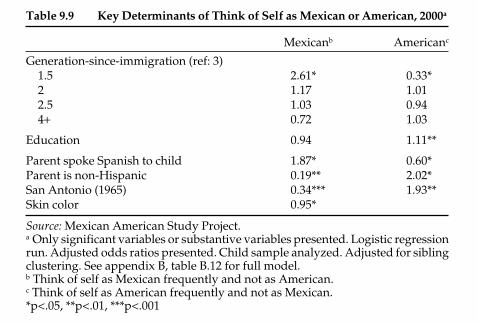
and expect me to speak Spanish.” The other end of the social gatheringspectrum involved a Mexican-origin majority, such as holiday celeb-rations. One respondent said he felt most Mexican “around a bunch ofother Mexicans.” The next two most common responses were listening toMexican music or speaking Spanish, both typical of social gatherings. Otherresponses were less frequent and included mentions of food and socialstatus. Responses for the parental and child generations were similar,except the child generation was much more likely to mention Mexicanimmigrant coworkers, needing to translate at work, and interactions withimmigrants suggesting that the new immigration had a greater effect inreinforcing ethnicity among the adult children.
We ran two regressions to examine the factors associated with oftenthinking of oneself as only Mexican or as American. Table 9.9 shows thatthose who often thought of themselves as Americans were more likely tobe more educated. Thus it appears that greater education implies greaterattachment to a national identity than an ethnic one. Additionally, we find,as expected, that immigrants were most likely to consider themselvesMexican and least likely to consider themselves American, as were thosegrowing up with speaking Spanish and those with a non-Hispanic parent.Angelenos also differed from San Antonians in thinking of themselves asmore Mexican and less American. Last, darker skin respondents were lesslikely to see themselves as Mexicans. This result is the opposite of whatwe would expect and is one of the few instances in which skin color hada significant effect on a dependent variable.
228 Generations of Exclusion
Table 9.9 Key Determinants of Think of Self as Mexican or American, 2000a
Mexicanb Americanc
Generation-since-immigration (ref: 3)1.5 2.61* 0.33*2 1.17 1.012.5 1.03 0.944+ 0.72 1.03
Education 0.94 1.11**
Parent spoke Spanish to child 1.87* 0.60*Parent is non-Hispanic 0.19** 2.02*San Antonio (1965) 0.34*** 1.93**Skin color 0.95*
Source: Mexican American Study Project.a Only significant variables or substantive variables presented. Logistic regressionrun. Adjusted odds ratios presented. Child sample analyzed. Adjusted for siblingclustering. See appendix B, table B.12 for full model.b Think of self as Mexican frequently and not as American.c Think of self as American frequently and not as Mexican.*p<.05, **p<.01, ***p<.001
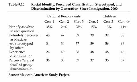
white in subsequent generations-since-immigration supports racializa-tion theories.
Perceived Race, Stereotyping, and Discrimination
We also asked our respondents about how others perceived them, whichgets at another, perhaps more important, dimension of race, which is gen-erally believed to be based on physical appearance. For blacks, it is basedon having at least one drop of African blood. The vast majority of AfricanAmericans, however, are identifiable based on physical appearance. Indeed,racial discrimination often depends on one’s physical appearance, especiallyin the important first impressions made by potential employers or in otherconsequential social interactions. Race is presumably based on physicalappearance for Asians also, but the extent of consistency between self-identification and identification by others is less than for African Americansand in the same range as Latinos.29 Thus, Latinos are distinguished as aseparate group to the same extent as Asians. Racial identities generallymirror those made in general society, and individuals are socialized tounderstand how others categorize them.
The second row of table 9.10 shows the extent to which our respon-dents believe they are definitely perceived as Mexican by others. Abouthalf (48 percent) of the immigrants believe they are and the percentagesdecline somewhat with each subsequent generation. By the fourth gener-ation, more than a third (38 percent) sense that they are definitely perceived
Ethnic Identity 231
Table 9.10 Racial Identity, Perceived Classification, Stereotyped, andDiscrimination by Generation-Since-Immigration, 2000
Original Respondents Children
Gen. 1 Gen. 2 Gen. 3 Gen. 2 Gen. 3 Gen. 4+Identify as white 38% 26% 28% 15% 13% 11%in race question
Definitely perceived 48 47 39 39 39 38as Mexican
Are stereotyped 34 34 37 59 56 66by others
Experience 24 40 38 48 48 46discrimination
Perceive “a great 36 38 37 37 35 37deal” of groupdiscrimination
Source: Mexican American Study Project.
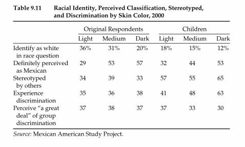
persons were less likely to identify as white, more likely to be perceivedas Mexican, and more likely to experience stereotyping and discrimination.Differences in stereotyping are not well correlated with skin color, perhapsbecause the question can be interpreted about stereotyping of the groupand not the individual respondent. The same goes for group discrimination.For the most part, the correlation is strong and suggests that darker personswere more discriminated against and saw themselves as nonwhite, thoughthe percentage of light-colored Mexican Americans also identifying asnonwhite and perceiving discrimination is substantial as well, certainlygreater than for European Americans.
Factors Affecting Racial Identity and Perceived DiscriminationTable 9.12 presents the odds ratios for determinants of whether respon-dents identified as white and reported experiencing discrimination. Wepresent the coefficients for variables that are statistically significant andfor generation-since-immigration and education. Interestingly, column 1results demonstrate that only one significant variable determined whetherrespondents identified as white, the comparison of Los Angeles and SanAntonio. Mexican Americans who grew up in San Antonio were more thanfive times as likely to identify as white as their counterparts in Los Angeles.This reveals a regional context of racial identity that is widely differentiatedbetween the two cities and probably between Texas and California. Thisalso reflects a well-accepted understanding that the Chicano political
234 Generations of Exclusion
Table 9.11 Racial Identity, Perceived Classification, Stereotyped, and Discrimination by Skin Color, 2000
Original Respondents Children
Light Medium Dark Light Medium Dark
Identify as white 36% 31% 20% 18% 15% 12%in race question
Definitely perceived 29 53 57 32 44 53as Mexican
Stereotyped 34 39 33 57 55 65by others
Experience 35 36 38 41 48 63discrimination
Perceive “a great 37 38 37 37 33 30deal” of groupdiscrimination
Source: Mexican American Study Project.
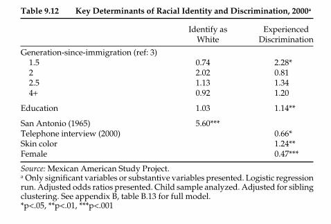
movement of the 1960s, which pursued a racialized identity rather thanan assimilationist strategy, as we described in chapter 4, became moreentrenched and accepted in Los Angeles than in San Antonio.
Angelenos and San Antonians are equally likely to report experiencesof discrimination. Many Mexican Americans, in Texas especially, wereconscious of discrimination but were nevertheless more likely to identifyas white. The idea of Mexicans as white but distinguished from so-calledAnglos, seems to be a locally accepted identity derived from the strategiesof Mexican American leaders of claiming whiteness to overcome their race-based exclusion. Reporting a white racial identity for Mexican Americansis not inconsistent with experiencing racial discrimination.
The second column of table 9.12 shows that the 1.5 generation was morelikely than the U.S.-born to experience discrimination, even thoughnearly all of them were at least partially educated and socialized in theUnited States. This may have to do with language characteristics that fur-ther distinguish them from non-Hispanics, including accent and a highcomfort level with Spanish. Also, more educated persons are generallymore likely to report discrimination. That may reflect that they are morelikely to have contact and compete with whites in the labor market or per-haps it reveals a more heightened sense that discrimination limits theiropportunities. Respondents interviewed over the telephone were abouttwo-thirds (.66) as likely to report experiences with discrimination. Thisprobably reflects the fact that they had mostly moved out of the LosAngeles or San Antonio area, suggesting that discrimination, or at least
Ethnic Identity 235
Table 9.12 Key Determinants of Racial Identity and Discrimination, 2000a
Identify as ExperiencedWhite Discrimination
Generation-since-immigration (ref: 3)1.5 0.74 2.28*2 2.02 0.812.5 1.13 1.344+ 0.92 1.20
Education 1.03 1.14**
San Antonio (1965) 5.60***Telephone interview (2000) 0.66*Skin color 1.24**Female 0.47***
Source: Mexican American Study Project.a Only significant variables or substantive variables presented. Logistic regressionrun. Adjusted odds ratios presented. Child sample analyzed. Adjusted for siblingclustering. See appendix B, table B.13 for full model.*p<.05, **p<.01, ***p<.001

Politics 259
Regression Analysis of Immigration Attitudes Last we examine what best pre-dicts having positive attitudes toward immigration (using the compositemeasure of attitudes in the last row on table 10.12). This is shown on table10.13. Not surprisingly, immigrants (generation 1.5) have significantly morepositive attitudes toward immigration than other generations. This mayreflect the fact that the less educated are more likely to directly compete withimmigrants in the labor market and thus would probably be inclined towant greater restrictions on immigration. Similarly, competition for hous-ing and schools from immigrants may be seen as negatively affecting costand quality of housing and education. More educated Mexican Americansalso have significantly more positive attitudes than the less educated. Thechildren of homeowners had less positive attitudes—this could be an effectof feeling that increased immigration negatively affects neighborhoods andconsequently home values. Apparently, this is a sentiment passed on fromparents to children. Children growing up in San Antonio had less positiveattitudes toward immigration, which probably reflects less exposure toimmigration. Interestingly, women also had less positive attitudes.
Figure 10.1 Agree that Mexicans Should be Able to Immigrate, 1965 and 2000
Source: Mexican American Study Project.
Generation-Since-Immigration
1
2
3
4+
Original Respondents
62%
50%
43% 56%
63%
72%
1965 2000
53%
54%
53%
2000
Children ofOriginalRespondents
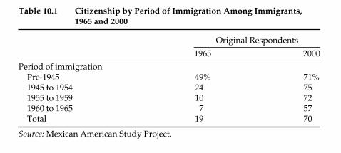
244 Generations of Exclusion
Voter Registration and Turnout
Although citizenship status is an issue for the Mexican-origin populationtoday, our sample was largely born in the United States and those whowere not have been United States residents for at least thirty years. Thusineligibility is not the primary reason for not voting or participating in the political process. Voting in the United States requires two steps for theU.S.-born, registration and actual voting. Table 10.2 shows that amongAmerican citizens, non-Hispanic whites have the highest registration andvoting rates, followed by blacks, then by Hispanics, and lastly by Asians.These numbers were self-reported by American citizens soon after theelections in 2000. Among adult American citizen Latinos, both voter reg-istration and turnout was low compared to other groups.35 Some, thoughnot all, of these differences may be explained by differences in age struc-ture and educational levels. Older and more educated people are morelikely to register and to vote.
Table 10.3 shows self-reported voting behavior from our data. Speci-fically, it presents voting registration and voting turnout rates in 1965 and2000 for original respondents and their children. In surveys of this type,overreporting is the rule, especially if much time has expired between the
Table 10.1 Citizenship by Period of Immigration Among Immigrants,1965 and 2000
Original Respondents
1965 2000
Period of immigrationPre-1945 49% 71%1945 to 1954 24 751955 to 1959 10 721960 to 1965 7 57Total 19 70
Source: Mexican American Study Project.
Table 10.2 Registered and Voted by Race, 2000a
Registered Voted
Hispanics 57% 45%Non-Hispanic whites 72 62Blacks 67 57Asians 52 43
Source: U.S. Bureau of the Census (2002).a Among general population of U.S. citizens.
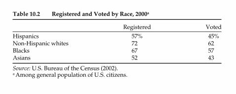
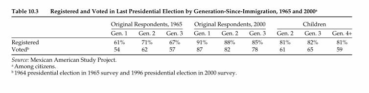
Table 10.3 Registered and Voted in Last Presidential Election by Generation-Since-Immigration, 1965 and 2000a
Original Respondents, 1965 Original Respondents, 2000 Children
Gen. 1 Gen. 2 Gen. 3 Gen. 1 Gen. 2 Gen. 3 Gen. 2 Gen. 3 Gen. 4+Registered 61% 71% 67% 91% 88% 85% 81% 82% 81%Votedb 54 62 57 87 82 78 61 65 59
Source: Mexican American Study Project.a Among citizens.b 1964 presidential election in 1965 survey and 1996 presidential election in 2000 survey.

246 Generations of Exclusion
election and the survey. Overreports of registering to vote can be expectedgiven that many Americans consider it their duty and lapses are oftenunjustifiable. Nonetheless, the figures in table 10.3 are useful in providingrelational differences among the generations. In 1965, voter registrationwas between 61 and 71 percent for all generational groups. It increasedbetween 1965 and 2000, when respondents in all generations reported voterregistration rates of greater than 80 percent (actual registration rates in thegeneral population are likely to be in the 60 to 70 percent range). The chil-dren of the original respondents were more likely to register to vote thantheir parents, at roughly the same age, were in 1965. However, by 2000, par-ents were more likely to register than their children. This might be an ageeffect because seniors are the most likely age group to vote.36
Voting, like registration, is overreported, especially in surveys takensome time after the vote is cast. For example, more than half (54 to 62 per-cent) of the eligible original respondents reported voting in 1964. However,78 percent or more reported voting in 1996, but only 59 to 65 percent ofthe children did. Thus, the elderly original respondents were thus clearlymore likely to vote than their children, in both elections. These numbersindicate that 80 to 90 percent reported voting out of those registered tovote. Figures of actual voting do not therefore appear to be as exagger-ated as those for registration because data based on exit poll data showedthat more than 80 percent of registered Latinos voted in the 1996 elec-tion.37 Among original respondents and children, there is no well-definedgenerational pattern.
We conducted regression analysis to predict reported voting in the1996 election. The results in table 10.4 show that the 1.5 generation, thosewho arrived in the United States as children, was much less likely tovote than the third generation. There are no other significant differencesby generation-since-immigration in voting. Each subsequent generation
Table 10.4 Key Determinants of Voting in 1996 Presidential Election, 2000a
Voted in 1996
Generation-since-immigration (ref: 3)1.5 0.27*2 0.872.5 0.824 0.95
Education 1.30***
Source: Mexican American Study Project.a Only significant variables or substantive variables presented. Logistic regressionrun. Adjusted odds ratios presented. Child sample analyzed. Adjusted for siblingclustering. See appendix B, table B.14 for full model.*p<.05, ***p<.001
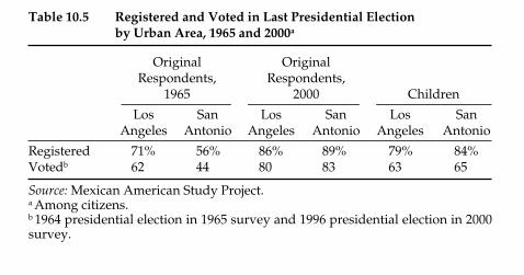
Table 10.6 Party Affiliation by Generation-Since-Immigration, 2000
Original Respondents Children
Gen. 1 Gen. 2 Gen. 3 Gen. 2 Gen. 3 Gen. 4+Democrat 78% 80% 69% 56% 54% 62%Republican 5 6 11 20 16 15Independent 10 10 12 15 21 14Other 7 4 8 9 9 9
Source: Mexican American Study Project.
248 Generations of Exclusion
Table 10.5 Registered and Voted in Last Presidential Election by Urban Area, 1965 and 2000a
Original Original Respondents, Respondents,
1965 2000 Children
Los San Los San Los San Angeles Antonio Angeles Antonio Angeles Antonio
Registered 71% 56% 86% 89% 79% 84%Votedb 62 44 80 83 63 65
Source: Mexican American Study Project.a Among citizens.b 1964 presidential election in 1965 survey and 1996 presidential election in 2000survey.
family and other values make them self-professed conservative or, asDe Sipio calls them, “proto-Republicans.”41 Indeed, Republicans haverecently made inroads in capturing the Latino vote. They have shown thatthe presumed allegiance of Mexican Americans to the Democratic Partyis questionable.42 On the other hand, though Mexican Americans are con-servative on moral issues, entrepreneurialism, support for the military,and the death penalty, these issues rank as less important to them thanothers that make them closer to the Democrats. These include educationand social services spending and the appropriate role and scope of thegovernment.43 Generational differences for Mexican Americans thuscapture the extent of stability or malleability of the Mexican Americanvote.44
Table 10.6 shows that fully 69 to 80 percent of the original respondentsconsidered themselves Democrats in 2000 versus only 54 to 62 percent ofthe children’s generation. For the original respondents, the third generationwas less Democratic than the other two generations. Among the children,
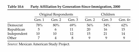
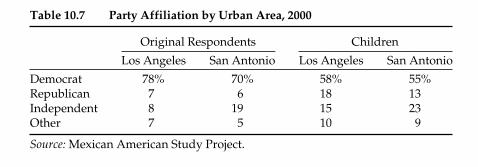
Politics 249
however, the fourth generation was the most Democratic, but the differ-ences were not large in either cohort. On the other hand, only 5 or 6 percentof the original respondents in the first and second generations—versus11 percent of the third generation—considered themselves Republican.Most of the non-Democrats considered themselves Independent or thirdparty and generational differences were not significant in either category.Many of the children of the original respondents had become Republicans.Interestingly, it was the second generation that had become the mostRepublican, the opposite of the pattern for their parents’ generation.Fully 20 percent of the second generation among children were Repub-lican and another 24 percent reported being Independent or anotherparty.
Where between 5 and 11 percent of the original respondents consideredthemselves Republicans in 2000, fully 15 to 20 percent of their children did.From the original respondents to their children, the proportion Republicangrew four times between immigrants and their second-generation chil-dren, more than two times from the second to the third generation, andalmost 50 percent from the third to the fourth generation. We suspect thatif we had comparable 1965 data about which party respondents consid-ered themselves, the intergenerational partisan shift would have beeneven more pronounced. We do have data on voting for president, whichsuggests great change.
Table 10.7, showing partisan data by urban area, indicates that bothoriginal respondents and their children in Los Angeles were more likelyto be Democrat than in San Antonio. Yet those in San Antonio were notmore likely to be Republican. Rather they described themselves moreoften as Independents, which may simply indicate dissatisfaction withthe political process rather than a particular ideology.
Presidential Voting, 1964 and 2000
Partisanship in actual voting is often quite different from declared parti-sanship. Many more of both original respondents and children voted
Table 10.7 Party Affiliation by Urban Area, 2000
Original Respondents Children
Los Angeles San Antonio Los Angeles San Antonio
Democrat 78% 70% 58% 55%Republican 7 6 18 13Independent 8 19 15 23Other 7 5 10 9
Source: Mexican American Study Project.
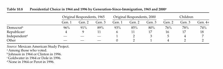
Table 10.8 Presidential Choice in 1964 and 1996 by Generation-Since-Immigration, 1965 and 2000a
Original Respondents, 1965 Original Respondents, 2000 Children
Gen. 1 Gen. 2 Gen. 3 Gen. 1 Gen. 2 Gen. 3 Gen. 2 Gen. 3 Gen. 4+Democratb 96% 91% 89% 93% 85% 80% 76% 78% 74%Republicanc 4 9 11 6 11 17 16 17 18Independentd — — — 1 2 3 5 4 7Other — — — 0 2 1 4 2 2
Source: Mexican American Study Project.a Among those who voted.b Johnson in 1964 or Clinton in 1996.c Goldwater in 1964 or Dole in 1996.d None in 1964 or Perot in 1996.

Table 10.10 Key Determinants of Voted Republican in 1996 and Identify Republican, 2000a
Voted Identify Republican Republican
Generation-Since-Immigration (ref: 3)1.5 0.96 0.662 2.23 3.21*2.5 1.28 2.07*4+ 1.33 1.18
Education 1.05 1.08
Father’s education 1.15**
Parent voted in 1964 (ref: voted Democrat)Voted Republican 4.36** 3.95**Did not vote 0.53*
Source: Mexican American Study Project.aOnly significant variables or substantive variables presented. Logistic regressionrun. Adjusted odds ratios presented. Child sample analyzed. Adjusted for siblingclustering. See appendix B, table B.15 for full model.*p<.05, **p<.01
252 Generations of Exclusion
Table 10.9 Presidential Choice in 1964 and 1996 by Urban Area, 1965 and 2000a
Original Original Respondents, Respondents,
1965 2000 Children
Los San Los San Los San Angeles Antonio Angeles Antonio Angeles Antonio
Democratb 91% 93% 86% 80% 77% 74%Republicanc 9 7 10 17 15 23Independentd — — 3 1 6 3Other — — 1 2 2 1
Source: Mexican American Study Project.a Among those who voted.b Johnson in 1964 or Clinton in 1996.c Goldwater in 1964 or Dole in 1996.d None in 1964 or Perot in 1996.

Politics 255
nistic nativist policies that seek to curtail or end immigration. Chapter 9showed that many Mexican-origin persons of all generations perceiveddiscrimination against members of their group.
Immigration Attitudes Ethnic attitudes about immigration vary widely byrace-ethnicity. Hispanics were much more pro-immigrant than whites andAfrican Americans.50 Based on a nationwide Gallup Poll about immigra-tion, Table 10.11 shows that the majority of non-Hispanic whites (52 per-cent) and blacks (66 percent) believed that immigrants hurt citizens bydriving down wages, but only 27 percent of Hispanics held such an opin-ion. Similarly, only 19 percent of whites and 30 percent of blacks agreedthat the United States should make it easier for illegal immigrants tobecome American citizens but fully 70 percent of Hispanics did.
But does this mean that all Mexican Americans, regardless of immigra-tion status, hold these attitudes? To what extent are pro-immigration atti-tudes merely due to self-interested immigrants or perhaps their second-generation children? The failure to disentangle most presentations ofimmigration attitudes by generation among Hispanics is certainly a prob-lem. One might expect later generations-since-immigration to hold atti-tudes about immigration similar to those of blacks and whites. This expec-tation is consistent with assimilation theory. On the other hand, there maybe an ethnic bloc that supported immigrants and that kept later-generationMexican Americans from holding widespread nativist sentiments.
Table 10.12 shows a surprising amount of ethnic cohesion aroundimmigration. It also reveals much less assimilation than assimilationtheorists might expect. Third- and fourth-generation voters had remark-ably similar preferences as immigrants and thus their attitudes on thesecontentious issues are quite distinct from those of non-Hispanics. Theoverall differences between Mexican American or Latino attitudes com-pared to either whites or blacks on immigration shown in table 10.11 thusseem to hold up regardless of generation-since-immigration. Table 10.12presents some signs of eroding support for immigration by later-generationMexican Americans compared to immigrants, but this was not always thecase. More important, their opinions were quite strong compared with those
Table 10.11 Immigration Attitudes by Race, 2005
Non-HispanicWhites Blacks Hispanics
Immigrants hurt economy by reducing wages 52% 66% 27%United States should make it easier for illegalsto become American citizens 19 30 70
Source: Gallup Poll (2005).
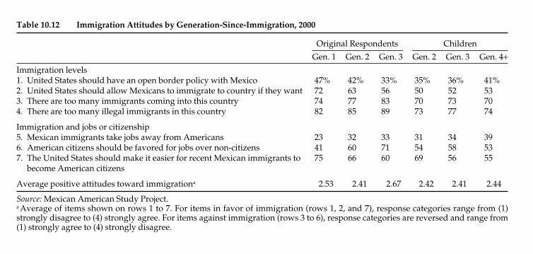
Table 10.12 Immigration Attitudes by Generation-Since-Immigration, 2000
Original Respondents Children
Gen. 1 Gen. 2 Gen. 3 Gen. 2 Gen. 3 Gen. 4+Immigration levels1. United States should have an open border policy with Mexico 47% 42% 33% 35% 36% 41%2. United States should allow Mexicans to immigrate to country if they want 72 63 56 50 52 533. There are too many immigrants coming into this country 74 77 83 70 73 704. There are too many illegal immigrants in this country 82 85 89 73 77 74
Immigration and jobs or citizenship5. Mexican immigrants take jobs away from Americans 23 32 33 31 34 396. American citizens should be favored for jobs over non-citizens 41 60 71 54 58 537. The United States should make it easier for recent Mexican immigrants to 75 66 60 69 56 55
become American citizens
Average positive attitudes toward immigrationa 2.53 2.41 2.67 2.42 2.41 2.44
Source: Mexican American Study Project.a Average of items shown on rows 1 to 7. For items in favor of immigration (rows 1, 2, and 7), response categories range from (1)strongly disagree to (4) strongly agree. For items against immigration (rows 3 to 6), response categories are reversed and range from(1) strongly agree to (4) strongly disagree.
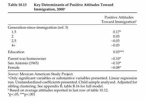
260 Generations of Exclusion
Affirmative Action Attitudes We asked one question about affirmativeaction in our survey (table 10.14). We found strong support in all genera-tions of Mexican Americans, but immigrants were the most supportive.There is no strong trend toward assimilation after that. The lack of a clearpattern, however, may not be surprising given that affirmative action,unlike immigration, is likely to affect all generations similarly. Among thegeneral population, Hispanics support for affirmative action (69 percent)is considerably more than that of non-Hispanic whites (44 percent), andsimilar to that of blacks (64 percent).
Language Attitudes Finally, we asked several attitudinal questions inrelation to the use of Spanish or English and bilingualism. Table 10.15shows that, for the most part, attitudes about language use do not clearlyfollow distinctions by generation-since-immigration. It does demonstrate,however, that the child cohort has more relaxed attitudes about whetherSpanish or English should be used. On all language items, whether pro-Spanish or pro-English, sentiments were always stronger in the parentgeneration, suggesting simultaneous feelings of both ethnic distinctive-ness and Americanness among that generation. In only one question didgeneration-since-immigration matter for both parents and children in anyconsistent way. Agreement with whether everyone should know English(row 4) increased with each succeeding generation-since-immigration in
Table 10.13 Key Determinants of Positive Attitudes Toward Immigration, 2000a
Positive Attitudes Toward Immigrationb
Generation-since-immigration (ref: 3)1.5 0.17*2 0.032.5 −0.034+ −0.03
Education 0.03***
Parent was homeowner −0.10*San Antonio (1965) −0.10*Female −0.08*
Source: Mexican American Study Project.a Only significant variables or substantive variables presented. Linear regressionrun. Unstandardized coefficients presented. Child sample analyzed. Adjusted forsibling clustering. See appendix B, table B.16 for full model.b Based on average attitudes reported in last row of table 10.12.*p<.05, ***p<.001
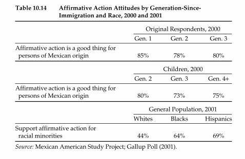
Politics 261
both samples. For the parent generation only, feelings that the local popu-lation should learn Spanish (row 5) tended to erode over succeedinggenerations-since-immigration. Nearly half (48 percent) of immigrants in the original sample believed that all residents in Los Angeles or SanAntonio, regardless of ancestry, should learn Spanish versus only one-third(33 percent) of the third generation.
ConclusionsOur evidence shows that though the participation of Mexican Americansin formal politics has been increasing through voting registration, partic-ipation continues to be low compared to whites and African Americans.We find no evidence of any patterned change with generation-since-immigration. We do, however, find that participation in the electoralprocess increased sharply from 1965 to 2000, especially in San Antonio.The weight of poll taxes in Texas and other factors that had discouragedMexican Americans from voting have since been largely lifted, extendingpolitical citizenship to Mexican Americans on a wide basis. The low overallrates of voter registration and participation among the Mexican Americanpopulation are partly driven by the immigrant generation, many of whomare not citizens and thus cannot vote. Among our surviving immigrant orig-inal respondents of the 1965 sample, fully 70 percent had become citizens by2000. However, among U.S.-born Mexican Americans, voting registrationand participation continues to be lower than for non-Hispanic whites, which
Table 10.14 Affirmative Action Attitudes by Generation-Since-Immigration and Race, 2000 and 2001
Original Respondents, 2000
Gen. 1 Gen. 2 Gen. 3
Affirmative action is a good thing forpersons of Mexican origin 85% 78% 80%
Children, 2000
Gen. 2 Gen. 3 Gen. 4+Affirmative action is a good thing forpersons of Mexican origin 80% 73% 75%
General Population, 2001
Whites Blacks Hispanics
Support affirmative action forracial minorities 44% 64% 69%
Source: Mexican American Study Project; Gallup Poll (2001).
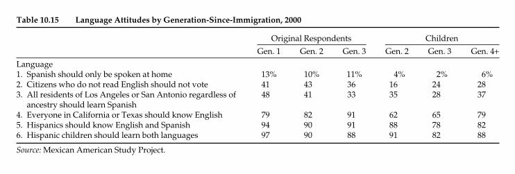
Table 10.15 Language Attitudes by Generation-Since-Immigration, 2000
Original Respondents Children
Gen. 1 Gen. 2 Gen. 3 Gen. 2 Gen. 3 Gen. 4+Language1. Spanish should only be spoken at home 13% 10% 11% 4% 2% 6%2. Citizens who do not read English should not vote 41 43 36 16 24 283. All residents of Los Angeles or San Antonio regardless of 48 41 33 35 28 37
ancestry should learn Spanish4. Everyone in California or Texas should know English 79 82 91 62 65 795. Hispanics should know English and Spanish 94 90 91 88 78 826. Hispanic children should learn both languages 97 90 88 91 82 88
Source: Mexican American Study Project.

268 Generations of Exclusion
sense of the American racial hierarchy. Our analysis shows that the lowlevels of education of later generations are unlikely to be attributable tothe alleged cultural deficiencies sometimes used to explain low educationfor immigrant children, such as poor ability in English or the lack of disci-pline or knowledge of American schools.
Figure 11.1 also shows a quite different pattern for language. Specifically,it reveals a slow but certain linear trend toward universal English mono-lingualism, which is consistent with reaching full assimilation on the lin-guistic dimension. Mexican Americans retain Spanish more than othergroups but do not keep it indefinitely. In the American context, the eventualloss of the ethnic language of immigrant ancestors is considered normaland even desirable, though bilingualism is common and often perceivedas indispensable in other societies. Virtually all other groups in United
Source: Mexican American Study Project.a From multivariate analysis among children.
Complete Assimilation
EnglishMonolingual
Years of Schooling Deficit
1 1.5 2 2.5 3 4 5
Lev
el o
f Ass
imila
tion
Generation-Since-Immigration
Figure 11.1 Educational and Linguistic Incorporation by Generation-Since-Immigration, 2000a
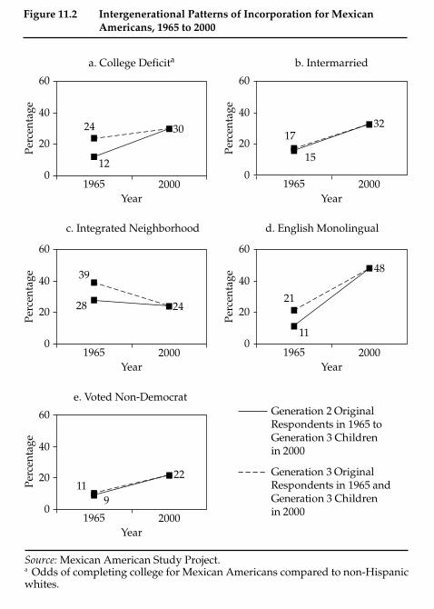
270 Generations of Exclusion
Source: Mexican American Study Project.a Odds of completing college for Mexican Americans compared to non-Hispanic whites.
a. College Deficita
1965
60
40
20
24
12
30
02000
Perc
enta
ge
Year
Year
Year
Year
Year
c. Integrated Neighborhood
1965
60
40
20
39
28 24
02000
Perc
enta
ge
b. Intermarried
1965
60
40
2017
15
32
02000
Perc
enta
ge
e. Voted Non-Democrat
1965
60
40
2011
9
22
02000
Perc
enta
ge
21
11
48
Generation 2 Original Respondents in 1965 to Generation 3 Children in 2000
Generation 3 Original Respondents in 1965 and Generation 3 Children in 2000
d. English Monolingual
1965
60
40
20
02000
Perc
enta
ge
Figure 11.2 Intergenerational Patterns of Incorporation for MexicanAmericans, 1965 to 2000
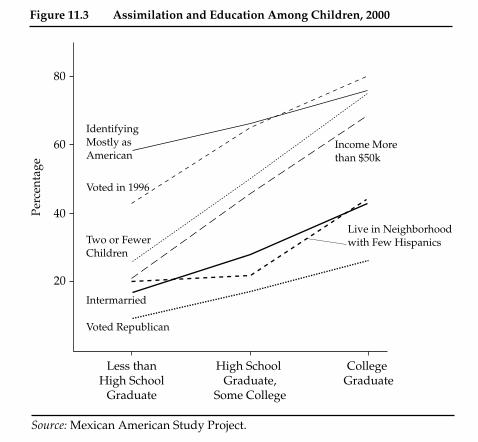
Conclusions 275
levels of schooling: less than high school, high school graduates with noor some college, and college graduates. Figure 11.3 demonstrates thatassimilation on each dimension increased with the level of schooling.16 Itshows, for example, that Mexican Americans with higher levels of educa-tion are more likely to have an American than an ethnic identity and aremore likely to vote, suggesting greater integration in the American polity.Relatedly, they are also more likely to vote Republican, suggesting thatthey are less committed to the usual party of the ethnic group. Their levelof education makes a notable difference in socioeconomic status (percent-age with incomes greater than $50,000)17 and exposure to other groups(percentage living in a neighborhood with 25 percent or fewer Hispanicsand percentage intermarried). Finally, they also have lower fertility (per-centage with two or fewer children), itself an important determinant ofthe educational level of the next generation.
These patterns are similar for the original respondent generation, thoughthe rates are often lower. We show these results in figure 11.4. For example,only about 5 percent of high school dropouts among the original respon-
Source: Mexican American Study Project.
IdentifyingMostly as American
Voted in 1996
Two or FewerChildren
Income Morethan $50k
Intermarried
Voted Republican
Live in Neighborhoodwith Few Hispanics
80
Less thanHigh School
Graduate
Perc
enta
ge
60
40
20
High School Graduate,
Some College
College Graduate
Figure 11.3 Assimilation and Education Among Children, 2000
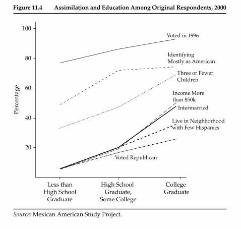
276 Generations of Exclusion
dents intermarried, versus more than 40 percent of college graduates.This compares with their children’s generation, in which about 15 percentof high school dropouts intermarried and nearly 40 percent of college grad-uates did. Thus, at the less-educated end, rates of intermarriage increasedabout three times. At the other, though, intermarriage rates have surpris-ingly remained stable from 1965 to 2000. To take two more examples, less-educated people in 1964 were much less likely to vote than in 1996 but werealso much more likely to live in integrated neighborhoods in 1964 than in1996.18 The most important point of figures 11.3 and 11.4, though, is toshow that assimilation is consistently related to education for two distinctgenerations of Mexican Americans and the persistence of educational dis-advantage largely predicts the group’s slow or halted assimilation.
Race, ethnicity, and class are thus deeply intertwined for MexicanAmericans. Low levels of education puts them largely in working classsectors (including low-level white-collar jobs) and the ethnic boundaries of
Figure 11.4 Assimilation and Education Among Original Respondents, 2000
Source: Mexican American Study Project.
IdentifyingMostly as American
Voted in 1996
Three or FewerChildren
Income Morethan $50k
Intermarried
Voted Republican
Live in Neighborhoodwith Few Hispanics
80
Less thanHigh School
Graduate
Perc
enta
ge
100
60
40
20
High School Graduate,
Some College
College Graduate

Table A.1 Descriptive Statistics for Dependent Variables in Regression Analysis, 2000a
Standard Sample Dependent Variables Mean Deviation Minimum Maximum Size Chapter
Years of education 13.26 2.18 2 17 758 5Occupational status 36.65 12.98 7 81 723 6Earnings $37,001 $26,142 $1,758 $167,962 698 6Family income $54,425 $37,301 $0 $171,672 725 6Net worth $51,190 $99,570 −$74,000 $1,000,000 700 6Hispanic in neighborhood (2000) 50.28 29.50 1 98 709 7Married to Hispanic 0.70 0.46 0 1 660 7Spanish proficiency 3.04 1.14 1 5 758 8Spanish birth name 2.98 1.17 1 5 758 8Children ever born 2.18 1.41 0 8 419 8Identify as Mexican 0.16 0.37 0 1 758 9Identify as Mexican American 0.43 0.49 0 1 758 9Identify as Hispanic or Latino 0.30 0.46 0 1 758 9Identify as American or other 0.11 0.32 0 1 758 9Think of self as Mexican frequently 0.19 0.39 0 1 758 9Think of self as American frequently 0.37 0.48 0 1 758 9Identify as white 0.15 0.35 0 1 758 9Experienced discrimination 0.46 0.50 0 1 758 9Voted in 1996 0.68 0.47 0 1 758 10Voted Republican 0.18 0.38 0 1 515 10Identify with Republican party 0.17 0.38 0 1 562 10Positive attitudes toward immigration 2.42 0.45 1 4 562 10
Source: Mexican American Study Project.a Child sample used in all regression analyses.
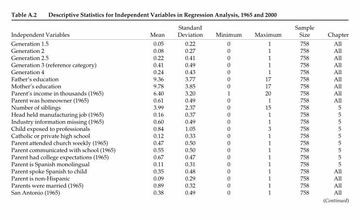
Table A.2 Descriptive Statistics for Independent Variables in Regression Analysis, 1965 and 2000
Standard Sample Independent Variables Mean Deviation Minimum Maximum Size Chapter
Generation 1.5 0.05 0.22 0 1 758 AllGeneration 2 0.08 0.27 0 1 758 AllGeneration 2.5 0.22 0.41 0 1 758 AllGeneration 3 (reference category) 0.41 0.49 0 1 758 AllGeneration 4 0.24 0.43 0 1 758 AllFather’s education 9.36 3.77 0 17 758 AllMother’s education 9.78 3.85 0 17 758 AllParent’s income in thousands (1965) 6.40 3.20 1 20 758 AllParent was homeowner (1965) 0.61 0.49 0 1 758 AllNumber of siblings 3.99 2.37 0 15 758 5Head held manufacturing job (1965) 0.16 0.37 0 1 758 5Industry information missing (1965) 0.60 0.49 0 1 758 5Child exposed to professionals 0.84 1.05 0 3 758 5Catholic or private high school 0.12 0.33 0 1 758 5Parent attended church weekly (1965) 0.47 0.50 0 1 758 5Parent communicated with school (1965) 0.55 0.50 0 1 758 5Parent had college expectations (1965) 0.67 0.47 0 1 758 5Parent is Spanish monolingual 0.11 0.31 0 1 758 5Parent spoke Spanish to child 0.35 0.48 0 1 758 AllParent is non-Hispanic 0.09 0.29 0 1 758 AllParents were married (1965) 0.89 0.32 0 1 758 AllSan Antonio (1965) 0.38 0.49 0 1 758 All
(Continued)
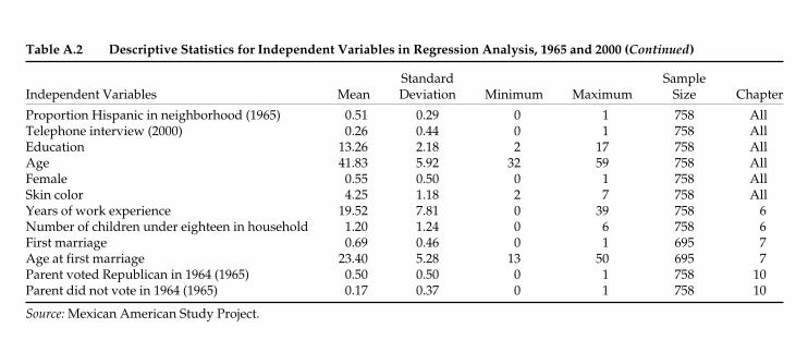
Proportion Hispanic in neighborhood (1965) 0.51 0.29 0 1 758 AllTelephone interview (2000) 0.26 0.44 0 1 758 AllEducation 13.26 2.18 2 17 758 AllAge 41.83 5.92 32 59 758 AllFemale 0.55 0.50 0 1 758 AllSkin color 4.25 1.18 2 7 758 AllYears of work experience 19.52 7.81 0 39 758 6Number of children under eighteen in household 1.20 1.24 0 6 758 6First marriage 0.69 0.46 0 1 695 7Age at first marriage 23.40 5.28 13 50 695 7Parent voted Republican in 1964 (1965) 0.50 0.50 0 1 758 10Parent did not vote in 1964 (1965) 0.17 0.37 0 1 758 10
Source: Mexican American Study Project.
Table A.2 Descriptive Statistics for Independent Variables in Regression Analysis, 1965 and 2000 (Continued)
Standard Sample Independent Variables Mean Deviation Minimum Maximum Size Chapter

297
Table B.1 Determinants of Locating and Interviewing OriginalRespondents, 2000 a
Located Interviewed
San Antonio 1.05 1.25Age 0.99 0.99Male 1.04 0.98Married 1.51* 1.42*Born in U.S. 1.34 1.07English interview 1.39 1.14Education 1.04 1.03Income (thousands) 1.05 1.00Homeowner 3.22*** 1.58**
Mean on dependent variable .789 .573Pseudo R2 .099 .025Log pseudo-likelihood −554 −794N 1193 1193
Source: Mexican American Study Project.a Logistic regression run. Adjusted odds ratios presented. Searched sample oforiginal respondents analyzed. Predictors based on 1965 characteristics.*p<.05, **p<.01; ***p<.001
Appendix B
Multivariate Analyses
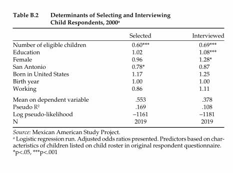
298 Appendix B
Table B.2 Determinants of Selecting and Interviewing Child Respondents, 2000a
Selected Interviewed
Number of eligible children 0.60*** 0.69***Education 1.02 1.08***Female 0.96 1.28*San Antonio 0.78* 0.87Born in United States 1.17 1.25Birth year 1.00 1.00Working 0.86 1.11
Mean on dependent variable .553 .378Pseudo R2 .169 .108Log pseudo-likelihood −1161 −1181N 2019 2019
Source: Mexican American Study Project.a Logistic regression run. Adjusted odds ratios presented. Predictors based on char-acteristics of children listed on child roster in original respondent questionnaire.*p<.05, ***p<.001

Appendix B 299
Table B.3 Determinants of Years of Education, 2000a
Years of Education
Unstandardized Robust Standard Coefficient Errors
Generation-since-immigration (ref: 3)1.5 1.46** 0.452 0.94** 0.312.5 0.40† 0.214+ −0.08 0.21
Parental status characteristicsFather’s education 0.10*** 0.03Mother’s education 0.08*** 0.02Parents’ income in thousands (1965) 0.06* 0.03Parent was homeowner (1965) 0.32† 0.19Number of siblings −0.08* 0.03Head held manufacturing job (1965) −0.26 0.23Industry information missing (1965) −0.45* 0.19
Childhood characteristicsChild exposed to professionals 0.23** 0.07Catholic or private high school 0.97*** 0.22Parent attended church weekly (1965) 0.45* 0.17Parent communicated with school (1965) 0.36* 0.18Parent had college expectations 0.04 0.17for children (1965)
Parent spoke Spanish to child 0.20 0.21Parent is Spanish monolingual −0.18 0.32Parent is non-Hispanic 0.21 0.30Parents were married (1965) −0.10 0.28
Residential characteristicsSan Antonio (1965) 0.07 0.21Proportion Hispanic in −0.24 0.28neighborhood (1965)
Telephone interview (2000) −0.05 0.18
Individual characteristicsFemale −0.26† 0.15Skin color 0.07 0.06Age 0.00 0.02
Intercept 10.69R2 .257N 758
Source: Mexican American Study Project.a Linear regression run. Child sample analyzed. Adjusted for sibling clustering:number of clusters = 482; robust standard errors are calculated.†p<.10, *p<.05, **p<.01, ***p<.001
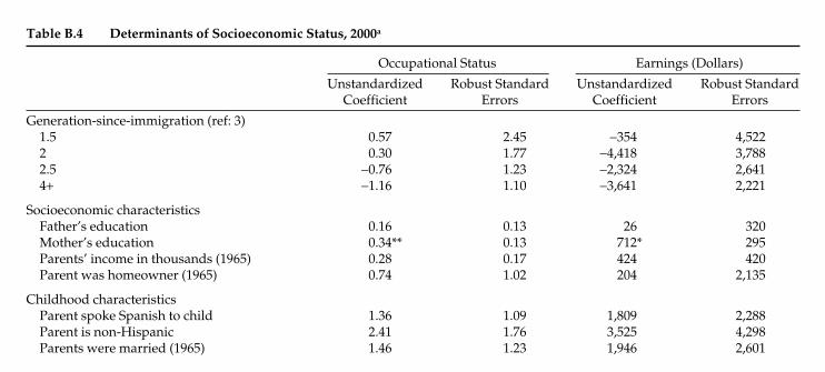
Table B.4 Determinants of Socioeconomic Status, 2000a
Occupational Status Earnings (Dollars)
Unstandardized Robust Standard Unstandardized Robust Standard Coefficient Errors Coefficient Errors
Generation-since-immigration (ref: 3)1.5 0.57 2.45 −354 4,5222 0.30 1.77 −4,418 3,7882.5 −0.76 1.23 −2,324 2,6414+ −1.16 1.10 −3,641 2,221
Socioeconomic characteristicsFather’s education 0.16 0.13 26 320Mother’s education 0.34** 0.13 712* 295Parents’ income in thousands (1965) 0.28 0.17 424 420Parent was homeowner (1965) 0.74 1.02 204 2,135
Childhood characteristicsParent spoke Spanish to child 1.36 1.09 1,809 2,288Parent is non-Hispanic 2.41 1.76 3,525 4,298Parents were married (1965) 1.46 1.23 1,946 2,601

Residential characteristicsSan Antonio (1965) 1.57 1.16 −1,053 2,273Proportion Hispanic in neighborhood (1965) 1.42 1.58 −3,807 3,466Telephone interview (2000) 1.28 1.02 7,479** 2,483
Human capitalEducation 2.99*** 0.22 4,043*** 486Years of work experienceb 0.09 0.06 240* 120Ageb
Individual characteristicsFemale 1.16 0.81 −12,676*** 1,717Skin color 0.26 0.33 742 685
Intercept −17.29 −29,402R2 .332 .261N 723 698
(Continued)
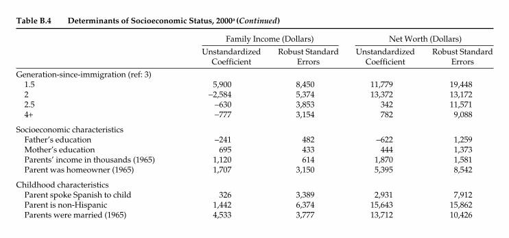
Generation-since-immigration (ref: 3)1.5 5,900 8,450 11,779 19,4482 −2,584 5,374 13,372 13,1722.5 −630 3,853 342 11,5714+ −777 3,154 782 9,088
Socioeconomic characteristicsFather’s education −241 482 −622 1,259Mother’s education 695 433 444 1,373Parents’ income in thousands (1965) 1,120 614 1,870 1,581Parent was homeowner (1965) 1,707 3,150 5,395 8,542
Childhood characteristicsParent spoke Spanish to child 326 3,389 2,931 7,912Parent is non-Hispanic 1,442 6,374 15,643 15,862Parents were married (1965) 4,533 3,777 13,712 10,426
Table B.4 Determinants of Socioeconomic Status, 2000a (Continued)
Family Income (Dollars) Net Worth (Dollars)
Unstandardized Robust Standard Unstandardized Robust Standard Coefficient Errors Coefficient Errors
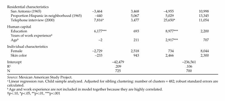
Residential characteristicsSan Antonio (1965) −3,464 3,468 −4,955 10,998Proportion Hispanic in neighborhood (1965) −440 5,067 5,029 13,345Telephone interview (2000) 7,816* 3,477 25,650* 11,054
Human capitalEducation 6,177*** 693 8,977*** 2,200Years of work experienceb
Ageb −2 211 2,917*** 707
Individual characteristicsFemale −2,729 2,518 734 8,044Skin color −233 943 2,466 2,300
Intercept −42,479 −236,561R2 .209 .106N 725 700
Source: Mexican American Study Project.a Linear regression run. Child sample analyzed. Adjusted for sibling clustering: number of clusters = 482; robust standard errors arecalculated.b Age and work experience are not included in model together because they are highly correlated.†p<.10, *p<.05, **p<.01, ***p<.001

304 Appendix B
Table B.5 Determinants of Hispanic Neighborhood, 2000a
Hispanic Neighborhood
Unstandardized Robust Standard Coefficient Errors
Generation-since-immigration (ref: 3)1.5 −1.59 5.332 −3.14 4.422.5 −0.06 2.684+ −3.50 2.64
Socioeconomic characteristicsFather’s education −0.51 0.34Mother’s education −0.62* 0.31Parents’ income in thousands (1965) −0.02 0.40Parent was homeowner (1965) 1.53 2.55
Childhood characteristicsParent spoke Spanish to child 1.77 2.64Parent is non-Hispanic −5.07 3.31Parents were married (1965) 3.89 3.53
Residential characteristicsSan Antonio (1965) 14.26*** 2.74Proportion Hispanic in 11.55** 3.78neighborhood (1965)
Telephone interview (2000) −14.13*** 2.46
Human capitalEducation −2.64*** 0.53
Individual characteristicsFemale −1.59 2.02Skin color −0.99 0.88Age −0.37 0.20Any children under −3.98† 2.09eighteen in household
Intercept 108.13R2 .329N 709
Source: Mexican American Study Project.a Linear regression run. Child sample analyzed. Adjusted for sibling clustering:number of clusters = 482; robust standard errors are calculated.b Age and work experience not included in model together because highly correlated.†p<.10, *p<.05, **p<.01, ***p<.001
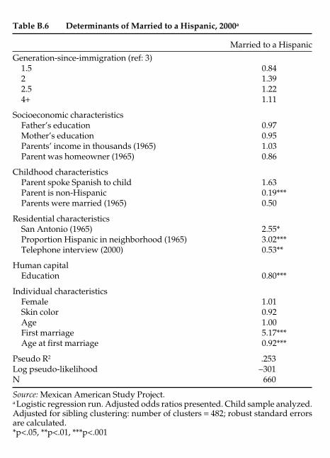
Appendix B 305
Table B.6 Determinants of Married to a Hispanic, 2000a
Married to a Hispanic
Generation-since-immigration (ref: 3)1.5 0.842 1.392.5 1.224+ 1.11
Socioeconomic characteristicsFather’s education 0.97Mother’s education 0.95Parents’ income in thousands (1965) 1.03Parent was homeowner (1965) 0.86
Childhood characteristicsParent spoke Spanish to child 1.63Parent is non-Hispanic 0.19***Parents were married (1965) 0.50
Residential characteristicsSan Antonio (1965) 2.55*Proportion Hispanic in neighborhood (1965) 3.02***Telephone interview (2000) 0.53**
Human capitalEducation 0.80***
Individual characteristicsFemale 1.01Skin color 0.92Age 1.00First marriage 5.17***Age at first marriage 0.92***
Pseudo R2 .253Log pseudo-likelihood −301N 660
Source: Mexican American Study Project.a Logistic regression run. Adjusted odds ratios presented. Child sample analyzed.Adjusted for sibling clustering: number of clusters = 482; robust standard errorsare calculated.*p<.05, **p<.01, ***p<.001
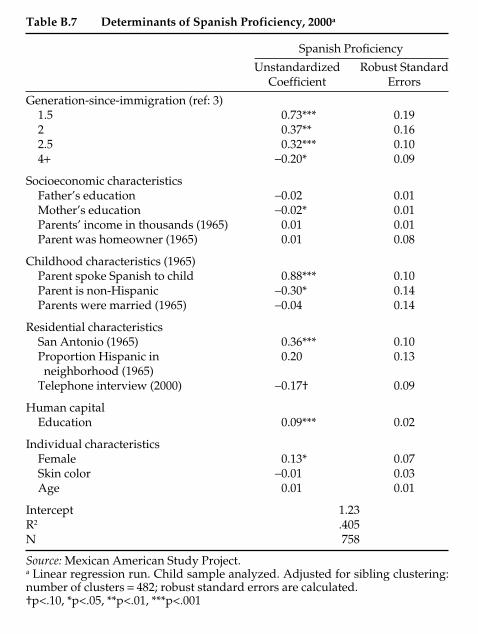
306 Appendix B
Table B.7 Determinants of Spanish Proficiency, 2000a
Spanish Proficiency
Unstandardized Robust Standard Coefficient Errors
Generation-since-immigration (ref: 3)1.5 0.73*** 0.192 0.37** 0.162.5 0.32*** 0.104+ −0.20* 0.09
Socioeconomic characteristicsFather’s education −0.02 0.01Mother’s education −0.02* 0.01Parents’ income in thousands (1965) 0.01 0.01Parent was homeowner (1965) 0.01 0.08
Childhood characteristics (1965)Parent spoke Spanish to child 0.88*** 0.10Parent is non-Hispanic −0.30* 0.14Parents were married (1965) −0.04 0.14
Residential characteristicsSan Antonio (1965) 0.36*** 0.10Proportion Hispanic in 0.20 0.13neighborhood (1965)
Telephone interview (2000) −0.17† 0.09
Human capitalEducation 0.09*** 0.02
Individual characteristicsFemale 0.13* 0.07Skin color −0.01 0.03Age 0.01 0.01
Intercept 1.23R2 .405N 758
Source: Mexican American Study Project.a Linear regression run. Child sample analyzed. Adjusted for sibling clustering:number of clusters = 482; robust standard errors are calculated.†p<.10, *p<.05, **p<.01, ***p<.001

Appendix B 307
Table B.8 Determinants of Spanish Birth Name, 2000a
Spanish Birth Name
Unstandardized Robust Standard Coefficient Errors
Generation-since-immigration (ref: 3)1.5 0.80*** 0.172 0.52** 0.172.5 0.58*** 0.124+ 0.11 0.10
Socioeconomic characteristicsFather’s education −0.06*** 0.01Mother’s education −0.02* 0.01Parents’ income in thousands (1965) 0.01 0.02Parent was homeowner (1965) −0.01 0.10
Childhood characteristicsParent is non-Hispanic −0.38* 0.16Parents were married (1965) −0.23† 0.12
Residential characteristicsSan Antonio (1965) 0.39** 0.11Proportion Hispanic in 0.16 0.16neighborhood (1965)
Telephone interview (2000) 0.03 0.10
Individual characteristicsFemale −0.05 0.08Skin color 0.01 0.04Age 0.01 0.01
Intercept 3.17R2 .192N 758
Source: Mexican American Study Project.aLinear regression run. Child sample analyzed. Adjusted for sibling clustering:number of clusters = 482; robust standard errors are calculated.†p<.10, *p<.05, **p<.01, ***p<.001

308 Appendix B
Table B.9 Determinants of Children Ever Born, 2000a
Children Ever Born
Unstandardized Robust Standard Coefficient Errors
Generation-since-immigration (ref: 3)1.5 −0.24 0.152 −0.12 0.142.5 0.16* 0.084+ 0.03 0.07
Socioeconomic characteristicsFather’s education −0.01 0.01Mother’s education −0.01 0.01Parents’ income in thousands (1965) −0.01 0.01Parent was homeowner (1965) 0.09 0.07
Childhood characteristicsParent spoke Spanish to child 0.13 0.07Parent is non-Hispanic −0.12 0.13Parents were married (1965) −0.06 0.08
Residential characteristicsSan Antonio (1965) 0.04 0.08Proportion Hispanic in −0.07 0.11neighborhood (1965)
Telephone interview (2000) 0.04 0.08
Human capitalEducation −0.08*** 0.01
Individual characteristicsSkin color −0.02 0.03Age 0.01* 0.01
Intercept 1.55N 758
Source: Mexican American Study Project.a Poisson regression run. Child sample analyzed. Adjusted for sibling clustering:number of clusters = 482; robust standard errors are calculated.*p<.05, ***p<.001
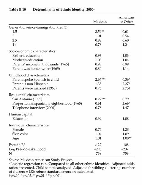
Appendix B 309
Table B.10 Determinants of Ethnic Identity, 2000a
American Mexican or Other
Generation-since-immigration (ref: 3)1.5 3.54** 0.612 1.01 0.542.5 0.88 0.604+ 0.76 1.24
Socioeconomic characteristicsFather’s education 0.96 1.03Mother’s education 1.03 1.04Parents’ income in thousands (1965) 0.98 0.99Parent was homeowner (1965) 0.80 1.14
Childhood characteristicsParent spoke Spanish to child 2.65*** 0.36*Parent is non-Hispanic 1.38 2.27*Parents were married (1965) 0.76 2.75†
Residential characteristicsSan Antonio (1965) 0.27*** 0.79Proportion Hispanic in neighborhood (1965) 0.61 2.66*Telephone interview (2000) 0.78 1.47
Human capitalEducation 0.99 1.08
Individual characteristicsFemale 0.74 1.28Skin color 1.04 1.09Age 1.01 1.08**
Pseudo R2 .122 108Log Pseudo-Likelihood −296 −237N 758 758
Source: Mexican American Study Project.a Logistic regression run. Compared to all other ethnic identities. Adjusted oddsratios presented. Child sample analyzed. Adjusted for sibling clustering: numberof clusters = 482; robust standard errors are calculated.†p<.10, *p<.05, **p<.01, ***p<.001
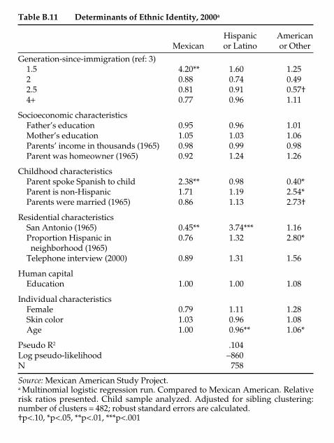
310 Appendix B
Table B.11 Determinants of Ethnic Identity, 2000a
Hispanic American Mexican or Latino or Other
Generation-since-immigration (ref: 3)1.5 4.20** 1.60 1.252 0.88 0.74 0.492.5 0.81 0.91 0.57†4+ 0.77 0.96 1.11
Socioeconomic characteristicsFather’s education 0.95 0.96 1.01Mother’s education 1.05 1.03 1.06Parents’ income in thousands (1965) 0.98 0.99 0.98Parent was homeowner (1965) 0.92 1.24 1.26
Childhood characteristicsParent spoke Spanish to child 2.38** 0.98 0.40*Parent is non-Hispanic 1.71 1.19 2.54*Parents were married (1965) 0.86 1.13 2.73†
Residential characteristicsSan Antonio (1965) 0.45** 3.74*** 1.16Proportion Hispanic in 0.76 1.32 2.80*neighborhood (1965)
Telephone interview (2000) 0.89 1.31 1.56
Human capitalEducation 1.00 1.00 1.08
Individual characteristicsFemale 0.79 1.11 1.28Skin color 1.03 0.96 1.08Age 1.00 0.96** 1.06*
Pseudo R2 .104Log pseudo-likelihood −860N 758
Source: Mexican American Study Project.a Multinomial logistic regression run. Compared to Mexican American. Relativerisk ratios presented. Child sample analyzed. Adjusted for sibling clustering:number of clusters = 482; robust standard errors are calculated.†p<.10, *p<.05, **p<.01, ***p<.001
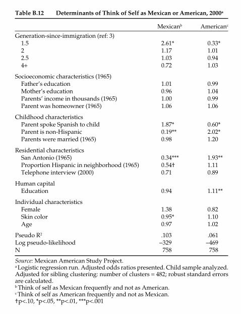
Appendix B 311
Table B.12 Determinants of Think of Self as Mexican or American, 2000a
Mexicanb Americanc
Generation-since-immigration (ref: 3)1.5 2.61* 0.33*2 1.17 1.012.5 1.03 0.944+ 0.72 1.03
Socioeconomic characteristics (1965)Father’s education 1.01 0.99Mother’s education 0.96 1.04Parents’ income in thousands (1965) 1.00 0.99Parent was homeowner (1965) 1.06 1.06
Childhood characteristicsParent spoke Spanish to child 1.87* 0.60*Parent is non-Hispanic 0.19** 2.02*Parents were married (1965) 0.98 1.20
Residential characteristicsSan Antonio (1965) 0.34*** 1.93**Proportion Hispanic in neighborhood (1965) 0.54† 1.11Telephone interview (2000) 0.71 0.89
Human capitalEducation 0.94 1.11**
Individual characteristicsFemale 1.38 0.82Skin color 0.95* 1.10Age 0.97 1.02
Pseudo R2 .103 .061Log pseudo-likelihood −329 −469N 758 758
Source: Mexican American Study Project.a Logistic regression run. Adjusted odds ratios presented. Child sample analyzed.Adjusted for sibling clustering: number of clusters = 482; robust standard errorsare calculated.b Think of self as Mexican frequently and not as American.c Think of self as American frequently and not as Mexican.†p<.10, *p<.05, **p<.01, ***p<.001

312 Appendix B
Table B.13 Determinants of Racial Identity and Discrimination, 2000a
Identify as Experienced White Discrimination
Generation-since-immigration (ref: 3)1.5 0.74 2.28*2 2.02 0.812.5 1.13 1.344+ 0.92 1.20
Socioeconomic characteristicsFather’s education 0.99 1.06*Mother’s education 1.04 0.94*Parents’ income in thousands (1965) 1.01 0.99Parent was homeowner (1965) 1.00 0.89
Childhood characteristicsParent spoke Spanish to child 0.68 0.99Parent is non-Hispanic 1.59 0.96Parents were married (1965) 1.05 0.77
Residential characteristicsSan Antonio (1965) 5.60*** 1.01Proportion Hispanic in neighborhood (1965) 0.76 1.08Telephone interview (2000) 0.90 0.66*
Human CapitalEducation 1.03 1.14**
Individual characteristicsFemale 1.50 0.47***Skin color 0.97 1.24**Age 1.03 1.01
Pseudo R2 .107 .070Log pseudo-likelihood −282 −486N 758 758
Source: Mexican American Study Project.a Logistic regression run. Adjusted odds ratios presented. Child sample analyzed.Adjusted for sibling clustering: number of clusters = 482; robust standard errorsare calculated.*p<.05, **p<.01, ***p<.001
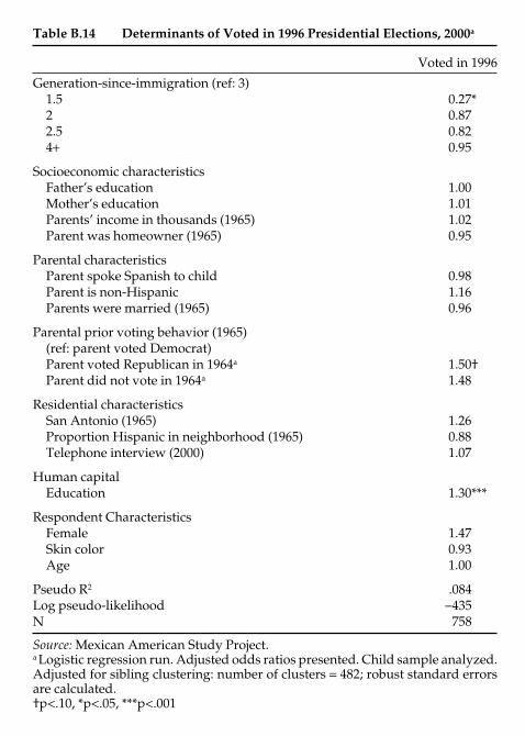
Appendix B 313
Table B.14 Determinants of Voted in 1996 Presidential Elections, 2000a
Voted in 1996
Generation-since-immigration (ref: 3)1.5 0.27*2 0.872.5 0.824+ 0.95
Socioeconomic characteristicsFather’s education 1.00Mother’s education 1.01Parents’ income in thousands (1965) 1.02Parent was homeowner (1965) 0.95
Parental characteristicsParent spoke Spanish to child 0.98Parent is non-Hispanic 1.16Parents were married (1965) 0.96
Parental prior voting behavior (1965)(ref: parent voted Democrat)Parent voted Republican in 1964a 1.50†Parent did not vote in 1964a 1.48
Residential characteristicsSan Antonio (1965) 1.26Proportion Hispanic in neighborhood (1965) 0.88Telephone interview (2000) 1.07
Human capitalEducation 1.30***
Respondent CharacteristicsFemale 1.47Skin color 0.93Age 1.00
Pseudo R2 .084Log pseudo-likelihood −435N 758
Source: Mexican American Study Project.a Logistic regression run. Adjusted odds ratios presented. Child sample analyzed.Adjusted for sibling clustering: number of clusters = 482; robust standard errorsare calculated.†p<.10, *p<.05, ***p<.001
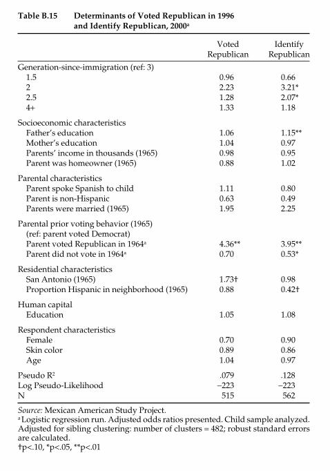
314 Appendix B
Table B.15 Determinants of Voted Republican in 1996 and Identify Republican, 2000a
Voted Identify Republican Republican
Generation-since-immigration (ref: 3)1.5 0.96 0.662 2.23 3.21*2.5 1.28 2.07*4+ 1.33 1.18
Socioeconomic characteristicsFather’s education 1.06 1.15**Mother’s education 1.04 0.97Parents’ income in thousands (1965) 0.98 0.95Parent was homeowner (1965) 0.88 1.02
Parental characteristicsParent spoke Spanish to child 1.11 0.80Parent is non-Hispanic 0.63 0.49Parents were married (1965) 1.95 2.25
Parental prior voting behavior (1965)(ref: parent voted Democrat)Parent voted Republican in 1964a 4.36** 3.95**Parent did not vote in 1964a 0.70 0.53*
Residential characteristicsSan Antonio (1965) 1.73† 0.98Proportion Hispanic in neighborhood (1965) 0.88 0.42†
Human capitalEducation 1.05 1.08
Respondent characteristicsFemale 0.70 0.90Skin color 0.89 0.86Age 1.04 0.97
Pseudo R2 .079 .128Log Pseudo-Likelihood −223 −223N 515 562
Source: Mexican American Study Project.a Logistic regression run. Adjusted odds ratios presented. Child sample analyzed.Adjusted for sibling clustering: number of clusters = 482; robust standard errorsare calculated.†p<.10, *p<.05, **p<.01
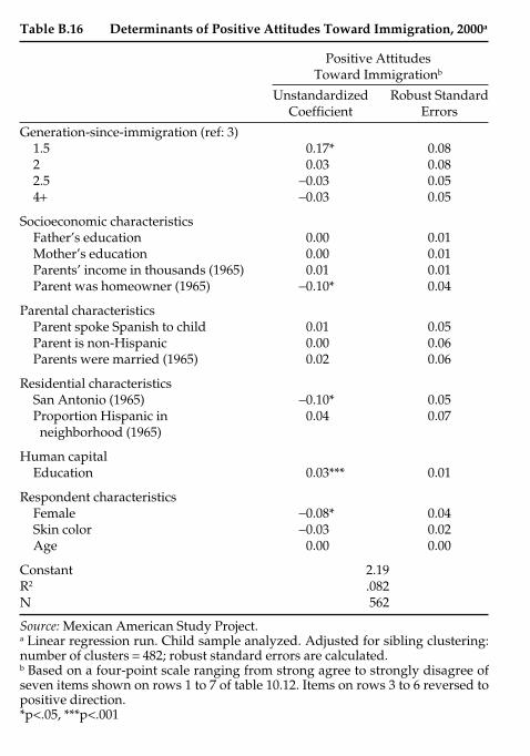
Appendix B 315
Table B.16 Determinants of Positive Attitudes Toward Immigration, 2000a
Positive Attitudes Toward Immigrationb
Unstandardized Robust Standard Coefficient Errors
Generation-since-immigration (ref: 3)1.5 0.17* 0.082 0.03 0.082.5 −0.03 0.054+ −0.03 0.05
Socioeconomic characteristicsFather’s education 0.00 0.01Mother’s education 0.00 0.01Parents’ income in thousands (1965) 0.01 0.01Parent was homeowner (1965) −0.10* 0.04
Parental characteristicsParent spoke Spanish to child 0.01 0.05Parent is non-Hispanic 0.00 0.06Parents were married (1965) 0.02 0.06
Residential characteristicsSan Antonio (1965) −0.10* 0.05Proportion Hispanic in 0.04 0.07neighborhood (1965)
Human capitalEducation 0.03*** 0.01
Respondent characteristicsFemale −0.08* 0.04Skin color −0.03 0.02Age 0.00 0.00
Constant 2.19R2 .082N 562
Source: Mexican American Study Project.a Linear regression run. Child sample analyzed. Adjusted for sibling clustering:number of clusters = 482; robust standard errors are calculated.b Based on a four-point scale ranging from strong agree to strongly disagree ofseven items shown on rows 1 to 7 of table 10.12. Items on rows 3 to 6 reversed topositive direction.*p<.05, ***p<.001