Experimental and Finite Element Analysis for a

American Institute of Aeronautics and Astronautics

1

Experimental and Finite Element Analysis for a Multifunctional Beam with Frequency-dependent

Viscoelastic Behavior

Ya Wang aand Daniel J. Inmanb a,b Department of Aerospace Engineering,

The University of Michigan, Ann Arbor, Michigan 48109-2140, USA

This paper investigates the frequency dependent viscoelastic dynamics of a five layer

multifunctional beam from finite element analysis and experimental validation. The frequency-

dependent behavior of the stiffness and damping of a viscoelastic material directly affects system

modal frequencies and damping, and results in complex vibration modes and differences in the

relative phase of vibration. A second order three parameter Golla-Hughes-McTavish (GHM) method

and a second order three fields Anelastic Displacement Fields (ADF) is used to implement the

viscoelastic material model, enabling the straightforward development of time domain and frequency

domain finite elements, and describing the frequency dependent viscoelastic behavior. Considering

the parameter identification, a strategy to estimate the fractional order of the time derivative and the

relaxation time is outlined. The curve-fitting aspects of both GHM and ADF show good agreement

with experimental data obtained from dynamic mechanics analysis. The performance of the finite

element of the layered multifunctional beam is verified through experimental model analysis.

Keywords: Finite Element Analysis, Golla-Hughes-McTavish, Anelastic Displacement Fields,

Frequency-dependent viscoelastic behavior

NOMENCLATURE

0

( ) : material modulus function : static or relaxed modulus

( ) , ( ) : modulus function for GHM and ADF models( ), ( ) : relax function and loss factor

'( ), "( ) : storage and

G A

G sG

G s G sH s

G Gη ω

ω ω loss modulus representing real and imagiary parts of complex modulus, , : finite element global mass, viscous damping and stiffness matrices of elastic systems

, , : finite element global mG G G

M D KM D K

0

ass, viscous damping and stiffness matrices of GHM model, , : finite element global mass, viscous damping and stiffness matrices of ADF model

, : static and dynamic stiffness, :

A A A

v v∞

M D KK K

q F finite element displacement and load vectors temperature

, , : parameters of the i-th mini-oscillator of GHM model : stress : strain : frequency : Laplace vari

i i i

s

θα ζ ω

σεω

=

able

a Post-doctoral Research Fellow, AIAA Member, [email protected]. b “Kelly” Johnson Collegiate Professor, Department Chairman, AIAA Fellow, [email protected].

Dow

nloa

ded

by U

NIV

ER

SIT

Y O

F M

ICH

IGA

N o

n A

pril

2, 2

014

| http

://ar

c.ai

aa.o

rg |

DO

I: 1

0.25

14/6

.201

3-16

40

54th AIAA/ASME/ASCE/AHS/ASC Structures, Structural Dynamics, and Materials Conference

April 8-11, 2013, Boston, Massachusetts

AIAA 2013-1640

Copyright © 2013 by Ya Wang, Dan Inman. Published by the American Institute of Aeronautics and Astronautics, Inc., with permission.

Structures, Structural Dynamics, and Materials and Co-located Conferences


2

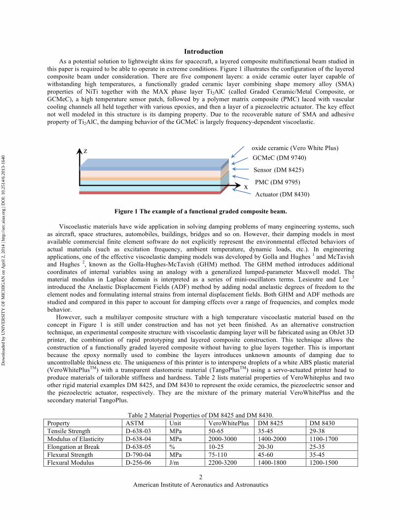
Introduction As a potential solution to lightweight skins for spacecraft, a layered composite multifunctional beam studied in

this paper is required to be able to operate in extreme conditions. Figure 1 illustrates the configuration of the layered composite beam under consideration. There are five component layers: a oxide ceramic outer layer capable of withstanding high temperatures, a functionally graded ceramic layer combining shape memory alloy (SMA) properties of NiTi together with the MAX phase layer Ti2AlC (called Graded Ceramic/Metal Composite, or GCMeC), a high temperature sensor patch, followed by a polymer matrix composite (PMC) laced with vascular cooling channels all held together with various epoxies, and then a layer of a piezoelectric actuator. The key effect not well modeled in this structure is its damping property. Due to the recoverable nature of SMA and adhesive property of Ti2AlC, the damping behavior of the GCMeC is largely frequency-dependent viscoelastic.

Figure 1 The example of a functional graded composite beam.

Viscoelastic materials have wide application in solving damping problems of many engineering systems, such as aircraft, space structures, automobiles, buildings, bridges and so on. However, their damping models in most available commercial finite element software do not explicitly represent the environmental effected behaviors of actual materials (such as excitation frequency, ambient temperature, dynamic loads, etc.). In engineering applications, one of the effective viscoelastic damping models was developed by Golla and Hughes 1 and McTavish and Hughes 2, known as the Golla-Hughes-McTavish (GHM) method. The GHM method introduces additional coordinates of internal variables using an analogy with a generalized lumped-parameter Maxwell model. The material modulus in Laplace domain is interpreted as a series of mini-oscillators terms. Lesieutre and Lee 3 introduced the Anelastic Displacement Fields (ADF) method by adding nodal anelastic degrees of freedom to the element nodes and formulating internal strains from internal displacement fields. Both GHM and ADF methods are studied and compared in this paper to account for damping effects over a range of frequencies, and complex mode behavior.

However, such a multilayer composite structure with a high temperature viscoelastic material based on the concept in Figure 1 is still under construction and has not yet been finished. As an alternative construction technique, an experimental composite structure with viscoelastic damping layer will be fabricated using an ObJet 3D printer, the combination of rapid prototyping and layered composite construction. This technique allows the construction of a functionally graded layered composite without having to glue layers together. This is important because the epoxy normally used to combine the layers introduces unknown amounts of damping due to uncontrollable thickness etc. The uniqueness of this printer is to intersperse droplets of a white ABS plastic material (VeroWhitePlusTM) with a transparent elastomeric material (TangoPlusTM) using a servo-actuated printer head to produce materials of tailorable stiffness and hardness. Table 2 lists material properties of VeroWhiteplus and two other rigid material examples DM 8425, and DM 8430 to represent the oxide ceramics, the piezoelectric sensor and the piezoelectric actuator, respectively. They are the mixture of the primary material VeroWhitePlus and the secondary material TangoPlus.

Table 2 Material Properties of DM 8425 and DM 8430.

Property ASTM Unit VeroWhitePlus DM 8425 DM 8430 Tensile Strength D-638-03 MPa 50-65 35-45 29-38 Modulus of Elasticity D-638-04 MPa 2000-3000 1400-2000 1100-1700 Elongation at Break D-638-05 % 10-25 20-30 25-35 Flexural Strength D-790-04 MPa 75-110 45-60 35-45 Flexural Modulus D-256-06 J/m 2200-3200 1400-1800 1200-1500

GCMeC (DM 9740) z

x

oxide ceramic (Vero White Plus)

Sensor (DM 8425)

PMC (DM 9795)

Actuator (DM 8430)

Dow

nloa

ded

by U

NIV

ER

SIT

Y O

F M

ICH

IGA

N o

n A

pril

2, 2

014

| http

://ar

c.ai

aa.o

rg |

DO

I: 1

0.25

14/6

.201

3-16

40


3

Table 3 displays two flexible materials DM 9740 and DM 9795 to represent the viscoelastic layer GCMeC and the vascular PMC layer, respectively. They are the combination of the primary material TangoPlus and the secondary material VeroWhitePlus.

Table 3 Material Properties of DM940 and DM 9795. Property ASTM Unit DM 9740 DM 9795 Tensile Strength D-412 MPa 1.3-1.8 8.5-10.0 Elongation at Break D-412 % 110-130 35-45 Tensile Tear Resistance D-624-Die C N/mm 5.5-7.5 41-44 Hardness Shore A D-2240 35-40 92-95

Finite Element Methods for Layered Composite Beam with Incorporated Viscoelastic Materials As shown in Figure 1, there are five component layers under consideration: the piezoelectric actuator layer (DM

8430), the PMC base beam (DM 9795), the high temperature sensor layer (DM 8425), the GCMeC viscoelastic layer (DM 9740), and the oxide ceramic constraint layer (Vero White Plus). Matrices and vectors associated with each layer but base layer are denoted with subscripts p, s, v and c, respectively. Nodes in the cross section are denoted using the global coordinate system located at the center of the left end of the base beam, and relative coordinate systems located at the bottom of each viscoelastic and piezoelectric layer. In order to faciliate beam modeling with hybrid damping treatments, the following assumptions are made:

1) The viscoelatic layer is augmented with the inclusion of a shear angle associated with transverse shear in addition to Euler-Bernoulli hypotheses.

2) The other four layers but viscoelatic layer are assumed to be elastic; Euler-Bernoulli bending assumption applies; Transverse and rotatory cross-section inertia are included.

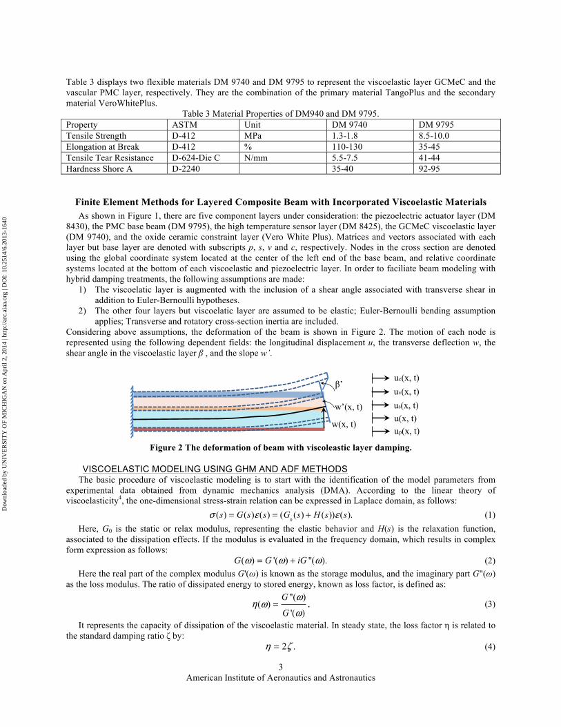
Considering above assumptions, the deformation of the beam is shown in Figure 2. The motion of each node is represented using the following dependent fields: the longitudinal displacement u, the transverse deflection w, the shear angle in the viscoelastic layer β , and the slope w’.

Figure 2 The deformation of beam with viscoleastic layer damping.

VISCOELASTIC MODELING USING GHM AND ADF METHODS The basic procedure of viscoelastic modeling is to start with the identification of the model parameters from

experimental data obtained from dynamic mechanics analysis (DMA). According to the linear theory of viscoelasticity4, the one-dimensional stress-strain relation can be expressed in Laplace domain, as follows:

σ (s) = G(s)ε (s) = (G0(s) + H (s))ε (s). (1)

Here, G0 is the static or relax modulus, representing the elastic behavior and H(s) is the relaxation function, associated to the dissipation effects. If the modulus is evaluated in the frequency domain, which results in complex form expression as follows:

( ) '( ) ''( ).G G iGω ω ω= + (2) Here the real part of the complex modulus G'(ω) is known as the storage modulus, and the imaginary part G"(ω)

as the loss modulus. The ratio of dissipated energy to stored energy, known as loss factor, is defined as:

"( )

( )'( ).G

G

ωη ω

ω= (3)

It represents the capacity of dissipation of the viscoelastic material. In steady state, the loss factor η is related to the standard damping ratio ζ by:

2 .η ζ= (4)

w(x, t)

w’(x, t)

β’

u(x, t)us(x, t)uv(x, t)

up(x, t)

uc(x, t)

Dow

nloa

ded

by U

NIV

ER

SIT

Y O

F M

ICH

IGA

N o

n A

pril

2, 2

014

| http

://ar

c.ai

aa.o

rg |

DO

I: 1

0.25

14/6

.201

3-16

40


4

However, η(ω) is not useful by itself in predicting transient or broad band responses of viscoelastic systems. The plots of complex modulus (storage modulus and loss modulus) or loss factor versus frequency are obtained from the DMA test of the viscoelastic material. These plots are then curve fit for modal parameter identification. Thus, in literature, the focus of the viscoelastic modeling is given on development of material modulus function G(s).

The modulus function derived from GHM method is given by:

2

0 2 21

2( ) ( )(1 ).

2

G

G

Nk k

kk k k k

s sG s G s

s s

ζ ωα

ζ ω ω=

+= +

+ +∑ (5)

Here NG is the number of mini-oscillator terms represented by three positive parameters (αk, ζk, ωk,). The modulus function can be expressed in complex forms, by simply making s iω= . Thus, the storage modulus (real part) developed by the GHM method becomes:

2 2 2 2 2 2

0 2 2 2 2 2 21

( ( ) 4 )'( ) (1 ).

( ) 4

G

G

Nk k k k

k k k k

G Gα ω ω ω ζ ω ω

ωω ω ζ ω ω=

− += +

− +∑ (6)

The loss modulus (imaginary part) from the GHM method yields:

3

0 2 2 2 2 2 21

2''( )

( ) 4.

G

G

Nk k k

k k k k

G Gα ζ ω ω

ωω ω ζ ω ω=

=− +

∑ (7)

The material modulus function developed by the ADF method is represented by:

0 2 2

1

( ) (1 ).A

A

N

kk k

sG s G

ω=

= + Δ+Ω

∑ (8)

Here NA is the number of anelastic displacement fields, represented by Ωk, the inverse of the characteristic relaxation time at constant deformation, and Δk, the relaxation magnitude. Decompose the modulus function in complex form, leads to the expression of the storage modulus by the ADF method:

2

0 21

( / )'( ) (1 )

( / ).

1A

A

Nk

kk k

G Gω

ωω=

Ω= + Δ

+ Ω∑ (9)

The loss modulus from the ADF method becomes:

2

1

/''( )

( / ).

1A

A

Nk

r kk k

G Gω

ωω=

Ω= Δ

+ Ω∑ (10)

Therefore, the material parameter determination is carried out by formulating an optimization problem in which the objective function represents the difference between the experimental data points and the corresponding model predictions. The numbers of design variables, for the GHM and ADF method are 1+3NG and 1+2NA, respectively.

FINITE ELEMENT MATRICES OF VISCOELASTIC CONSTRAINED LAYER SANDWICH BEAM The two-dimensional finite element formulation of this three-layer sandwich beam is derived in this section,

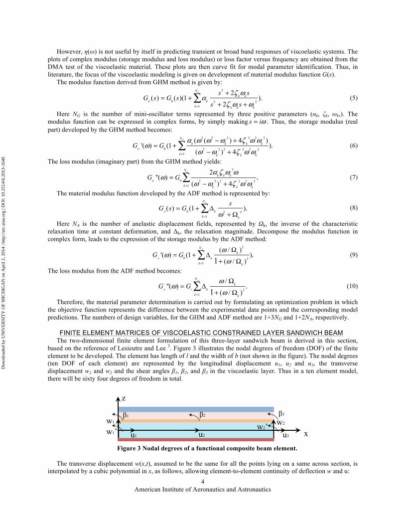
based on the reference of Lesieutre and Lee 3. Figure 3 illustrates the nodal degrees of freedom (DOF) of the finite element to be developed. The element has length of l and the width of b (not shown in the figure). The nodal degrees (ten DOF of each element) are represented by the longitudinal displacement u1, u2 and u3, the transverse displacement w1 and w2 and the shear angles β1, β2, and β3 in the viscoelastic layer. Thus in a ten element model, there will be sixty four degrees of freedom in total.

Figure 3 Nodal degrees of a functional composite beam element.

The transverse displacement w(x,t), assumed to be the same for all the points lying on a same across section, is

interpolated by a cubic polynomial in x, as follows, allowing element-to-element continuity of deflection w and u:

w2’ w2

β3

w1’w1

xu3u1 u2

β2β1

z

Dow

nloa

ded

by U

NIV

ER

SIT

Y O

F M

ICH

IGA

N o

n A

pril

2, 2

014

| http

://ar

c.ai

aa.o

rg |

DO

I: 1

0.25

14/6

.201

3-16

40


5

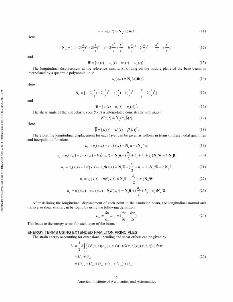
w = w(x, t) = Nw(x)w(t). (11)

Here

Nw = [ 1− 3(

x

l)2 + 2(

x

l)3 x − 2

x2

l+

x3

l 23(

x

l)2 − 2(

x

l)3 −

x2

l+

x3

l 2]. (12)

and ' '

1 1 2 2 .[ ( ) ( ) ( ) ( )]Tw t w t w t w t=w (13) The longitudinal displacement at the reference axis, u0(x,t), lying on the middle plane of the base beam, is

interpolated by a quadratic polynomial in x: u0

(x, t) = Nu(x)u(t). (14)

Here

2 2 2,[1 3( ) 2( ) 4( ) 4( ) 2( ) ]

x x x x x x

l l l l l l= − + − − +uN (15)

and

1 2 3[ ( ) ( ) ( )] .Tu t u t u t=u (16) The shear angle of the viscoelastic core β(x,t) is interpolated consistently with u(x,t): .( , ) ( ) ( )x t x tβ = uN β (17)

Here

1 2 3 ,[ ( ) ( ) ( )]Tt t tβ β β=β (18) Therefore, the longitudinal displacement for each layer can be given as follows in terms of these nodal quantities

and interpolation functions:

0 ,( , ) '( , ) 'bu u x t zw x t z= − = −u wN u N w (19)

0 ,( , ) '( , ) ( , ) ( )

2b

c v s v c v

hu u x t zw x t h x t h h z hβ= − − = − + + + −u w uN u N 'w N β (20)

0 ,( , ) '( , ) ( , ) ( )

2b

v v s v v

hu u x t zw x t z x t h z zβ= − − = − + + −u w uN u N 'w N β (21)

0 ,( , ) '( , ) ( )

2b

s s

hu u x t zw x t z= − = − +u wN u N 'w (22)

0 ( , ) '( , ) ( , ) ( ) .

2b

p v p p

hu u x t zw x t h x t h zβ= − − = + + −u wN u N 'w (23)

After defining the longitudinal displacement of each point in the sandwich beam, the longitudinal normal and

transverse shear strains can be found by using the following definition:

., ( )xx xz

u u w

x z xε ε

∂ ∂ ∂= = +∂ ∂ ∂

(24)

This leads to the energy terms for each layer of the beam.

ENERGY TERMS USING EXTENDED HAMILTON PRINCIPLES The strain energy accounting for extensional, bending and shear effects can be given by:

2 2

0

1( ( , )( ( , , )) ( , )( ( , , )) )

2

( )

l

xx xz

z

E G

E b Ec Ev Es Ep Gv

U b E x z x z t G x z x z t dzdx

U U

U U U U U U

ε ε= +

= +

= + + + + +

∫ ∫ (25)

Dow

nloa

ded

by U

NIV

ER

SIT

Y O

F M

ICH

IGA

N o

n A

pril

2, 2

014

| http

://ar

c.ai

aa.o

rg |

DO

I: 1

0.25

14/6

.201

3-16

40


6

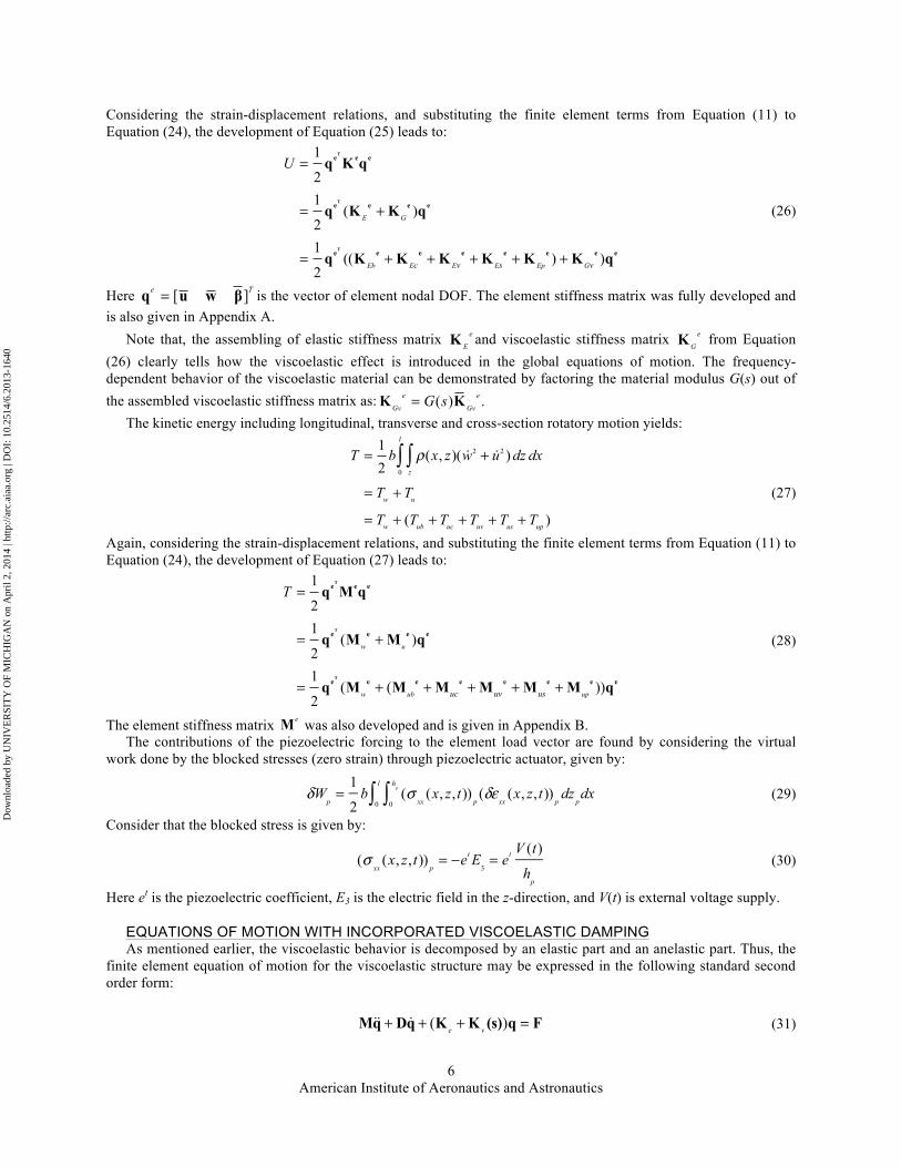
Considering the strain-displacement relations, and substituting the finite element terms from Equation (11) to Equation (24), the development of Equation (25) leads to:

1

21

( )21

(( ) )2

E G

Eb E E E Ep Gc v s v

U =

= +

= + + + + +

T

T

T

e e e

e e e e

e e e e e e e e

q K q

q K K q

q K K K K K K q

(26)

Here [ ]e T=q u w β is the vector of element nodal DOF. The element stiffness matrix was fully developed and is also given in Appendix A.

Note that, the assembling of elastic stiffness matrix e

EK and viscoelastic stiffness matrix e

GK from Equation (26) clearly tells how the viscoelastic effect is introduced in the global equations of motion. The frequency-dependent behavior of the viscoelastic material can be demonstrated by factoring the material modulus G(s) out of the assembled viscoelastic stiffness matrix as: ( ) .e e

Gv GvG s=K K The kinetic energy including longitudinal, transverse and cross-section rotatory motion yields:

T =12b ρ(x, z)( w2 + u2 )dz dx

z∫

0

l

∫= Tw + Tu= Tw + (Tub + Tuc + Tuv + Tus + Tup )

(27)

Again, considering the strain-displacement relations, and substituting the finite element terms from Equation (11) to Equation (24), the development of Equation (27) leads to:

1

21

( )21

( ( ))2

w u

w ub upuc uv us

T =

= +

= + + + + +

T

T

T

e e e

e e e e

e e e e e e e e

q M q

q M M q

q M M M M M M q

(28)

The element stiffness matrix eM was also developed and is given in Appendix B. The contributions of the piezoelectric forcing to the element load vector are found by considering the virtual

work done by the blocked stresses (zero strain) through piezoelectric actuator, given by:

δW

p=

1

2b (σ

xx(x, z, t))

p0

hp∫0

l

∫ (δεxx

(x, z, t))pdz

pdx (29)

Consider that the blocked stress is given by:

(σ

xx(x, z, t))

p= −et E

3= et V (t)

hp

(30)

Here et is the piezoelectric coefficient, E3 is the electric field in the z-direction, and V(t) is external voltage supply.

EQUATIONS OF MOTION WITH INCORPORATED VISCOELASTIC DAMPING As mentioned earlier, the viscoelastic behavior is decomposed by an elastic part and an anelastic part. Thus, the

finite element equation of motion for the viscoelastic structure may be expressed in the following standard second order form:

Mq + D q + (K e +K v (s))q = F (31)

Dow

nloa

ded

by U

NIV

ER

SIT

Y O

F M

ICH

IGA

N o

n A

pril

2, 2

014

| http

://ar

c.ai

aa.o

rg |

DO

I: 1

0.25

14/6

.201

3-16

40


7

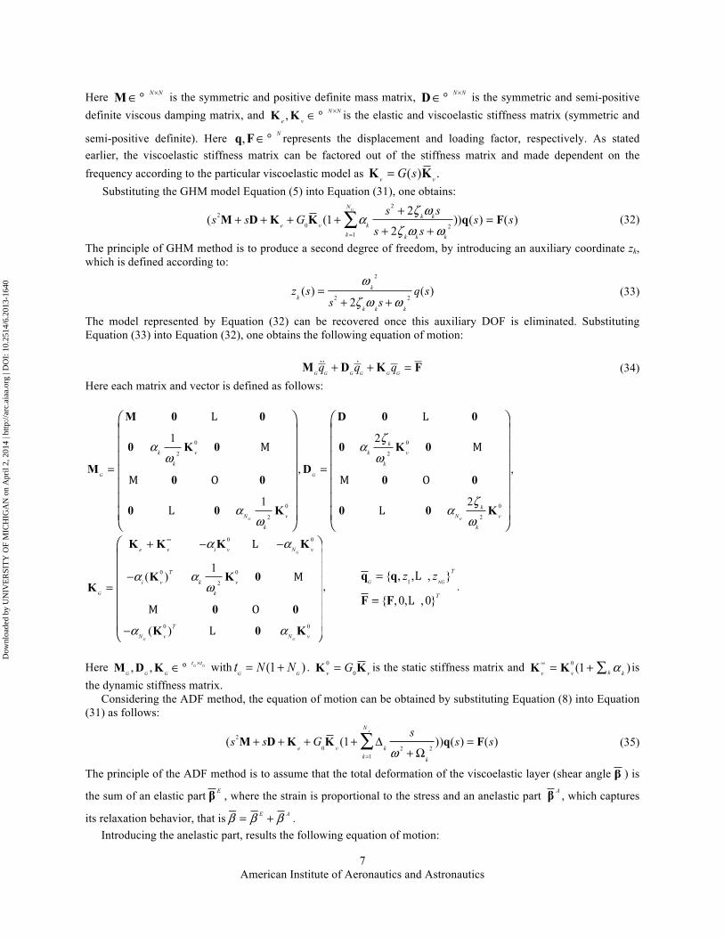
Here N N×∈M ° is the symmetric and positive definite mass matrix, N N×∈D ° is the symmetric and semi-positive definite viscous damping matrix, and , N N

e v

×∈K K ° is the elastic and viscoelastic stiffness matrix (symmetric and

semi-positive definite). Here , N∈q F ° represents the displacement and loading factor, respectively. As stated earlier, the viscoelastic stiffness matrix can be factored out of the stiffness matrix and made dependent on the frequency according to the particular viscoelastic model as ( ) .v vG s=K K

Substituting the GHM model Equation (5) into Equation (31), one obtains:

2

2

0 21

2( (1 )) ( ) ( )

2

GNk k

e v kk k k k

s ss s G s s

s s

ζ ωα

ζ ω ω=

++ + + + =

+ +∑M D K K q F (32)

The principle of GHM method is to produce a second degree of freedom, by introducing an auxiliary coordinate zk, which is defined according to:

z

k(s) =

ωk

2

s2 + 2ζkω

ks +ω

k

2q(s) (33)

The model represented by Equation (32) can be recovered once this auxiliary DOF is eliminated. Substituting Equation (33) into Equation (32), one obtains the following equation of motion:

MGqG+ D

GqG+K

GqG= F (34)

Here each matrix and vector is defined as follows:

0

2

0

2

1

1G

G

k v

k

N v

k

αω

αω

=

⎛ ⎞⎜ ⎟⎜ ⎟⎜ ⎟⎜ ⎟⎜ ⎟⎜ ⎟⎜ ⎟⎝ ⎠

M 0 0

0 K 0

M0 0

0 0 K

L

M

M O

L

,

0

2

0

2

2

2G

G

kk v

k

kN v

k

ζα

ω

ζα

ω

=

⎛ ⎞⎜ ⎟⎜ ⎟⎜ ⎟⎜ ⎟⎜ ⎟⎜ ⎟⎜ ⎟⎝ ⎠

D 0 0

0 K 0

D0 0

0 0 K

L

M

M O

L

,

0 0

0 0

2

0 0

1( )

( )

G

G G

G

e v i v N v

T

i v k v

k

T

N v N v

α α

α αω

α α

∞+ − −

−=

−

⎛ ⎞⎜ ⎟⎜ ⎟⎜ ⎟⎜ ⎟⎜ ⎟⎜ ⎟⎝ ⎠

K K K K

K K 0K

0 0

K 0 K

L

M

M O

L

, 1{ , , , }

{ ,0, , 0}

G NG

T

T

z z=

=

q q

F F

L

L.

Here , , G G

G G G

t t×∈M D K ° with (1 )G G

N Nt = + . 0

0v vG=K K is the static stiffness matrix and 0 (1 )kv v kα∞ = +∑K K is the dynamic stiffness matrix.

Considering the ADF method, the equation of motion can be obtained by substituting Equation (8) into Equation (31) as follows:

(s2M + sD + K

e+ G

0K

v(1+ Δ

k

s

ω 2 +Ωk

2)

k=1

NA

∑ )q(s) = F(s) (35)

The principle of the ADF method is to assume that the total deformation of the viscoelastic layer (shear angle β ) is

the sum of an elastic part Eβ , where the strain is proportional to the stress and an anelastic part Aβ , which captures

its relaxation behavior, that is β = β E + β A . Introducing the anelastic part, results the following equation of motion:

Dow

nloa

ded

by U

NIV

ER

SIT

Y O

F M

ICH

IGA

N o

n A

pril

2, 2

014

| http

://ar

c.ai

aa.o

rg |

DO

I: 1

0.25

14/6

.201

3-16

40


8

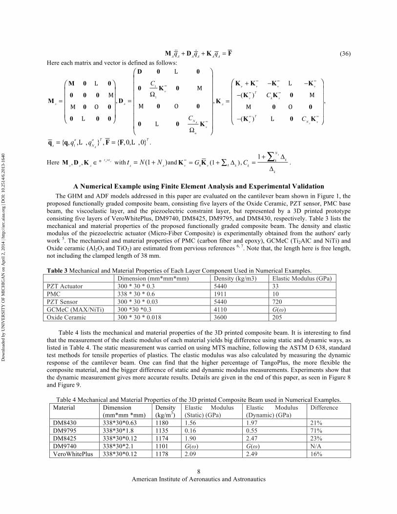
M AqA + DA

qA +K AqA = F (36) Here each matrix and vector is defined as follows:

A=

⎛ ⎞⎜ ⎟⎜ ⎟⎜ ⎟⎜ ⎟⎝ ⎠

M 0 0

0 0 0M

0 0

0 0 0

L

M

M O

L

,

1

1

A

A

v

N

v

n

C

C

∞

∞

Ω=

Ω

⎛ ⎞⎜ ⎟⎜ ⎟⎜ ⎟⎜ ⎟⎜ ⎟⎜ ⎟⎜ ⎟⎝ ⎠

D 0 0

0 K 0

D0 0

0 0 K

L

M

M O

L

,( )

( )A

A

e v v v

T

v k v

T

v N v

C

C

∞ ∞ ∞

∞ ∞

∞ ∞

+ − −

−=

−

⎛ ⎞⎜ ⎟⎜ ⎟⎜ ⎟⎜ ⎟⎝ ⎠

K K K K

K K 0K

0 0

K 0 K

L

M

M O

L

,

1{ , , , } , { ,0, ,0}A A

a a T T

Nq q= =q q F FL L .

Here , , A A

A A A

t t×∈M D K ° with (1 )A AN Nt = + and

0 (1 )kv v kG∞ = + Δ∑K K ,1 AN

kkk

k

C+ Δ

=Δ∑ .

A Numerical Example using Finite Element Analysis and Experimental Validation The GHM and ADF models addressed in this paper are evaluated on the cantilever beam shown in Figure 1, the

proposed functionally graded composite beam, consisting five layers of the Oxide Ceramic, PZT sensor, PMC base beam, the viscoelastic layer, and the piezoelectric constraint layer, but represented by a 3D printed prototype consisting five layers of VeroWhitePlus, DM9740, DM8425, DM9795, and DM8430, respectively. Table 3 lists the mechanical and material properties of the proposed functionally graded composite beam. The density and elastic modulus of the piezoelectric actuator (Micro-Fiber Composite) is experimentally obtained from the authors' early work 5. The mechanical and material properties of PMC (carbon fiber and epoxy), GCMeC (Ti2AlC and NiTi) and Oxide ceramic (Al2O3 and TiO2) are estimated from pervious references 6, 7. Note that, the length here is free length, not including the clamped length of 38 mm.

Table 3 Mechanical and Material Properties of Each Layer Component Used in Numerical Examples. Dimension (mm*mm*mm) Density (kg/m3) Elastic Modulus (GPa) PZT Actuator 300 * 30 * 0.3 5440 33 PMC 338 * 30 * 0.6 1911 10 PZT Sensor 300 * 30 * 0.03 5440 720 GCMeC (MAX/NiTi) 300 *30 *0.3 4110 G(ω) Oxide Ceramic 300 * 30 * 0.018 3600 205

Table 4 lists the mechanical and material properties of the 3D printed composite beam. It is interesting to find that the measurement of the elastic modulus of each material yields big difference using static and dynamic ways, as listed in Table 4. The static measurement was carried on using MTS machine, following the ASTM D 638, standard test methods for tensile properties of plastics. The elastic modulus was also calculated by measuring the dynamic response of the cantilever beam. One can find that the higher percentage of TangoPlus, the more flexible the composite material, and the bigger difference of static and dynamic modulus measurements. Experiments show that the dynamic measurement gives more accurate results. Details are given in the end of this paper, as seen in Figure 8 and Figure 9.

Table 4 Mechanical and Material Properties of the 3D printed Composite Beam used in Numerical Examples. Material Dimension

(mm*mm *mm) Density (kg/m3)

Elastic Modulus (Static) (GPa)

Elastic Modulus (Dynamic) (GPa)

Difference

DM8430 338*30*0.63 1180 1.56 1.97 21% DM9795 338*30*1.8 1135 0.16 0.55 71% DM8425 338*30*0.12 1174 1.90 2.47 23% DM9740 338*30*2.1 1101 G(ω) G(ω) N/A VeroWhitePlus 338*30*0.12 1178 2.09 2.49 16%

Dow

nloa

ded

by U

NIV

ER

SIT

Y O

F M

ICH

IGA

N o

n A

pril

2, 2

014

| http

://ar

c.ai

aa.o

rg |

DO

I: 1

0.25

14/6

.201

3-16

40


9

CURVE FITS FOR GHM AND ADF MODEL PARAMETER IDENTIFICATION As seen from Equations (34) and (35), the inclusion of the dissipative variables in the GHM and ADF models to

account for the viscoelastic behavior leads to augmented coupled systems of equations of motion in which the total number of DOF largely exceeds the number of structural DOF. Moreover, for both models, non-positive-definite inertia matrices are obtained. As result, numerical preprocessing is found to be necessary prior to the resolution of the equations for response analyses.

A positive-definite inertia matrix can be obtained for the GHM model by performing the spectral decomposition of the stiffness matrix related to the viscoelastic substructure 2. The null eigenvalues and corresponding eigenvectors are eliminated and, as result, fewer dissipative coordinates and a positive-definite viscoelastic matrix are obtained. As for the ADF model, it is not possible to obtain a positive-definite mass matrix by using the same approach. However, the problems entailed by the singularity can be avoided by performing an adequate transformation of augmented system of second-order equations into a state-space first-order form, the dimension of which is, in general, much smaller than that obtained for the GHM model 8.

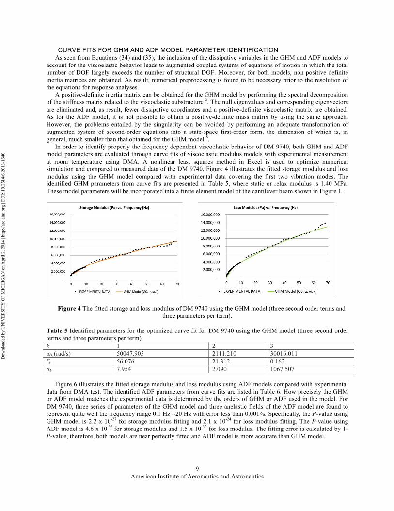
In order to identify properly the frequency dependent viscoelastic behavior of DM 9740, both GHM and ADF model parameters are evaluated through curve fits of viscoelastic modulus models with experimental measurement at room temperature using DMA. A nonlinear least squares method in Excel is used to optimize numerical simulation and compared to measured data of the DM 9740. Figure 4 illustrates the fitted storage modulus and loss modulus using the GHM model compared with experimental data covering the first two vibration modes. The identified GHM parameters from curve fits are presented in Table 5, where static or relax modulus is 1.40 MPa. These model parameters will be incorporated into a finite element model of the cantilever beam shown in Figure 1.

Figure 4 The fitted storage and loss modulus of DM 9740 using the GHM model (three second order terms and three parameters per term).

Table 5 Identified parameters for the optimized curve fit for DM 9740 using the GHM model (three second order terms and three parameters per term). k 1 2 3 ωk (rad/s) 50047.905 2111.210 30016.011 ζk 56.076 21.312 0.162 αk 7.954 2.090 1067.507

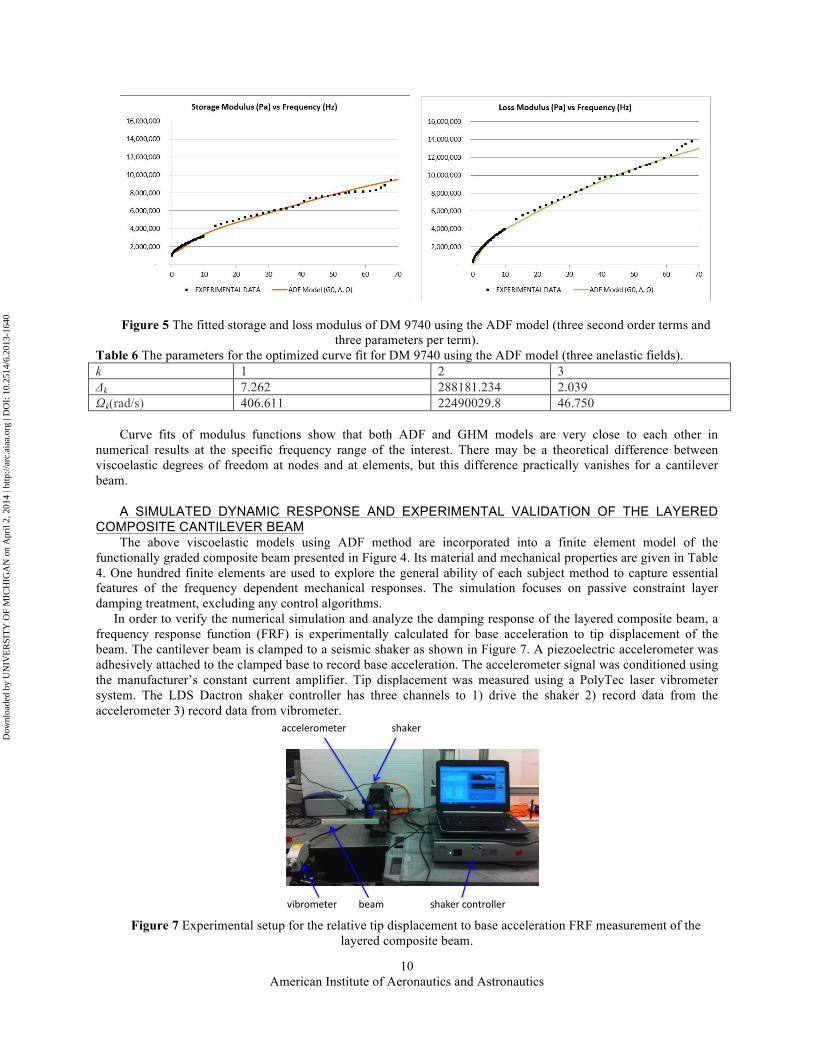
Figure 6 illustrates the fitted storage modulus and loss modulus using ADF models compared with experimental data from DMA test. The identified ADF parameters from curve fits are listed in Table 6. How precisely the GHM or ADF model matches the experimental data is determined by the orders of GHM or ADF used in the model. For DM 9740, three series of parameters of the GHM model and three anelastic fields of the ADF model are found to represent quite well the frequency range 0.1 Hz ~20 Hz with error less than 0.001%. Specifically, the P-value using GHM model is 2.2 x 10-27 for storage modulus fitting and 2.1 x 10-24 for loss modulus fitting. The P-value using ADF model is 4.6 x 10-36 for storage modulus and 1.5 x 10-32 for loss modulus. The fitting error is calculated by 1- P-value, therefore, both models are near perfectly fitted and ADF model is more accurate than GHM model.

Dow

nloa

ded

by U

NIV

ER

SIT

Y O

F M

ICH

IGA

N o

n A

pril

2, 2

014

| http

://ar

c.ai

aa.o

rg |

DO

I: 1

0.25

14/6

.201

3-16

40


10

Figure 5 The fitted storage and loss modulus of DM 9740 using the ADF model (three second order terms and three parameters per term).

Table 6 The parameters for the optimized curve fit for DM 9740 using the ADF model (three anelastic fields). k 1 2 3 Δk 7.262 288181.234 2.039 Ωk(rad/s) 406.611 22490029.8 46.750

Curve fits of modulus functions show that both ADF and GHM models are very close to each other in numerical results at the specific frequency range of the interest. There may be a theoretical difference between viscoelastic degrees of freedom at nodes and at elements, but this difference practically vanishes for a cantilever beam.

A SIMULATED DYNAMIC RESPONSE AND EXPERIMENTAL VALIDATION OF THE LAYERED COMPOSITE CANTILEVER BEAM

The above viscoelastic models using ADF method are incorporated into a finite element model of the functionally graded composite beam presented in Figure 4. Its material and mechanical properties are given in Table 4. One hundred finite elements are used to explore the general ability of each subject method to capture essential features of the frequency dependent mechanical responses. The simulation focuses on passive constraint layer damping treatment, excluding any control algorithms.

In order to verify the numerical simulation and analyze the damping response of the layered composite beam, a frequency response function (FRF) is experimentally calculated for base acceleration to tip displacement of the beam. The cantilever beam is clamped to a seismic shaker as shown in Figure 7. A piezoelectric accelerometer was adhesively attached to the clamped base to record base acceleration. The accelerometer signal was conditioned using the manufacturer’s constant current amplifier. Tip displacement was measured using a PolyTec laser vibrometer system. The LDS Dactron shaker controller has three channels to 1) drive the shaker 2) record data from the accelerometer 3) record data from vibrometer.

Figure 7 Experimental setup for the relative tip displacement to base acceleration FRF measurement of the

layered composite beam.

shaker

shaker controllerbeam

accelerometer

vibrometer

Dow

nloa

ded

by U

NIV

ER

SIT

Y O

F M

ICH

IGA

N o

n A

pril

2, 2

014

| http

://ar

c.ai

aa.o

rg |

DO

I: 1

0.25

14/6

.201

3-16

40


11

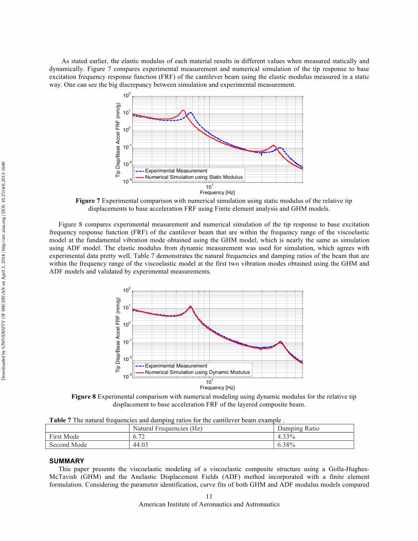
As stated earlier, the elastic modulus of each material results in different values when measured statically and

dynamically. Figure 7 compares experimental measurement and numerical simulation of the tip response to base excitation frequency response function (FRF) of the cantilever beam using the elastic modulus measured in a static way. One can see the big discrepancy between simulation and experimental measurement.

Figure 7 Experimental comparison with numerical simulation using static modulus of the relative tip

displacements to base acceleration FRF using Finite element analysis and GHM models.

Figure 8 compares experimental measurement and numerical simulation of the tip response to base excitation frequency response function (FRF) of the cantilever beam that are within the frequency range of the viscoelastic model at the fundamental vibration mode obtained using the GHM model, which is nearly the same as simulation using ADF model. The elastic modulus from dynamic measurement was used for simulation, which agrees with experimental data pretty well. Table 7 demonstrates the natural frequencies and damping ratios of the beam that are within the frequency range of the viscoelastic model at the first two vibration modes obtained using the GHM and ADF models and validated by experimental measurements.

Figure 8 Experimental comparison with numerical modeling using dynamic modulus for the relative tip

displacement to base acceleration FRF of the layered composite beam. Table 7 The natural frequencies and damping ratios for the cantilever beam example . Natural Frequencies (Hz) Damping Ratio First Mode 6.72 4.33% Second Mode 44.03 6.38%

SUMMARY This paper presents the viscoelastic modeling of a viscoelastic composite structure using a Golla-Hughes-

McTavish (GHM) and the Anelastic Displacement Fields (ADF) method incorporated with a finite element formulation. Considering the parameter identification, curve fits of both GHM and ADF modulus models compared

10110-3

10-2

10-1

100

101

102

Frequency [Hz]

Tip

Dis

p/Ba

se A

ccel

FR

F (m

m/g

)

Experimental MeasurementNumerical Simulation using Static Modulus

10110-3

10-2

10-1

100

101

102

Frequency [Hz]

Tip

Dis

p/Ba

se A

ccel

FR

F (m

m/g

)

Experimental MeasurementNumerical Simulation using Dynamic Modulus

Dow

nloa

ded

by U

NIV

ER

SIT

Y O

F M

ICH

IGA

N o

n A

pril

2, 2

014

| http

://ar

c.ai

aa.o

rg |

DO

I: 1

0.25

14/6

.201

3-16

40


12

with experimental data are presented. And a good agreement (less than 0.001% error) is reached. Continuing efforts are addressing the material modulus comparison of the GHM and the ADF model. There may be a theoretical difference between viscoelastic degrees of freedom at nodes and elements, but their numerical results are very close to each other at the specific frequency range of interest. With identified model parameters, numerical simulation is carried out to predict the damping behavior in its first two vibration modes. The experimental testing on the layered composite beam validates the numerical predication pretty well. Experimental results also show that elastic modulus measured from dynamic response yields more accurate results than static measurement, such as tensile testing, especially for flexible materials.

ACKNOWLEDGMENTS The authors gratefully acknowledge the support from the U.S. Air Force Office of Scientific Research under the

grant No FA-9550-09-1-0686 “Synthesis, Characterization and Modeling of Functionally Graded Hybrid Composites for Extreme Environments” monitored by Dr. David Stargel.

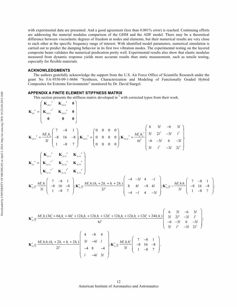
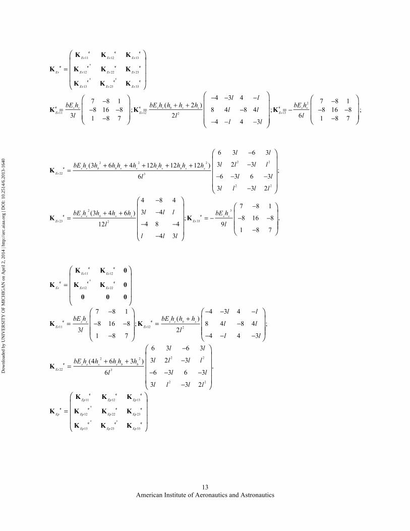
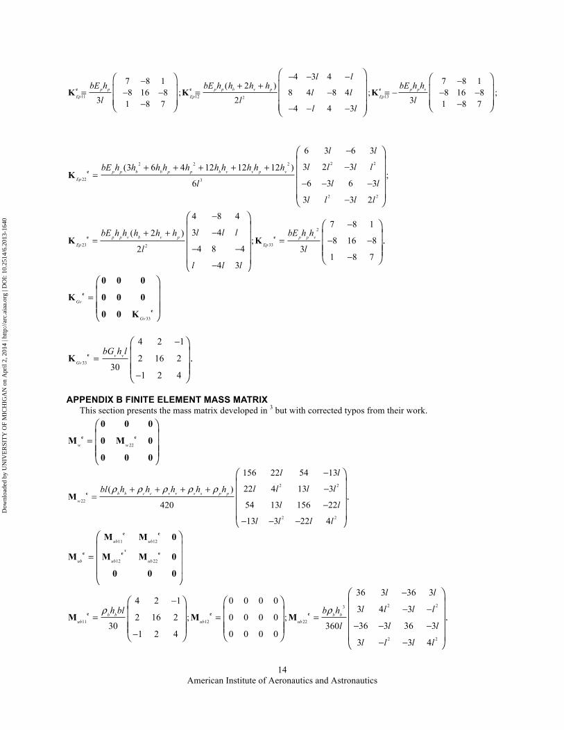
APPENDIX A FINITE ELEMENT STIFFNESS MATRIX This section presents the stiffness matrix developed in 3 with corrected typos from their work.

11 12

12 22

Eb Eb

Eb Eb Eb=

⎛ ⎞⎜ ⎟⎜ ⎟⎜ ⎟⎝ ⎠

T

e e

e e e

K K 0

K K K 0

0 0 0

2 23

11 12 22 3

2 2

6 3 6 37 8 1 0 0 0 0

3 2 38 16 8 ; 0 0 0 0 ;

6 3 6 33 61 8 7 0 0 0 0

3 3 2

.b b b bEb Eb Eb

l l

l l l lbE h bE h

l ll l

l l l l

−−

−= − − = =

− − −−

−

⎛ ⎞⎛ ⎞ ⎛ ⎞ ⎜ ⎟⎜ ⎟ ⎜ ⎟ ⎜ ⎟⎜ ⎟ ⎜ ⎟ ⎜ ⎟⎜ ⎟ ⎜ ⎟⎝ ⎠ ⎝ ⎠ ⎜ ⎟⎝ ⎠

e e eK K K

11 12 13

12 22 23

13 23 33

Ec Ec Ec

Ec Ec Ec Ec

Ec Ec Ec

=

⎛ ⎞⎜ ⎟⎜ ⎟⎜ ⎟⎝ ⎠

T

T T

e e e

e e e e

e e e

K K K

K K K K

K K K

K Ec11

e =bEchc3l

7 −8 1−8 16 −81 −8 7

⎛

⎝⎜⎜

⎞

⎠⎟⎟;K Ec12

e =bEchc (hb + 2hv + hc + 2hs )

2l 2

−4

8

−4

−3l

4l

−l

4

−8

4

−l

4l

−3l

⎛

⎝

⎜⎜⎜

⎞

⎠

⎟⎟⎟;K Ec13

e = −bEchchv3l

7 −8 1−8 16 −81 −8 7

⎛

⎝⎜⎜

⎞

⎠⎟⎟;

K Ec22

e =bEchc (3hb

2 + 6hbhc + 4hc2 +12hbhv +12hvhc +12hv

2 +12hbhs +12hshc +12hs2 + 24hvhs )

6l3

6 3l −6 3l3l 2l 2 −3l l 2

−6 −3l 6 −3l3l l 2 −3l 2l 2

⎛

⎝

⎜⎜⎜

⎞

⎠

⎟⎟⎟;

K Ec23

e =bEchchv (hb + 2hv + hc + 2hs )

2l 2

4

3l

−4

l

−8

−4l

8

−4l

4

l

−4

3l

⎛

⎝

⎜⎜⎜⎜

⎞

⎠

⎟⎟⎟⎟

;K Ec33

e =bEchchv

2

3l

7 −8 1−8 16 −81 −8 7

⎛

⎝⎜⎜

⎞

⎠⎟⎟.

Dow

nloa

ded

by U

NIV

ER

SIT

Y O

F M

ICH

IGA

N o

n A

pril

2, 2

014

| http

://ar

c.ai

aa.o

rg |

DO

I: 1

0.25

14/6

.201

3-16

40


13

11 12 13

12 22 23

13 23 33

Ev Ev Ev

Ev Ev Ev Ev

Ev Ev Ev

=

⎛ ⎞⎜ ⎟⎜ ⎟⎜ ⎟⎝ ⎠

T

T T

e e e

e e e e

e e e

K K K

K K K K

K K K

K Ev11

e =bEvhv3l

7 −8 1−8 16 −81 −8 7

⎛

⎝⎜⎜

⎞

⎠⎟⎟;K Ev12

e =bEvhv (hb + hv + 2hs )

2l 2

−4

8

−4

−3l

4l

−l

4

−8

4

−l

4l

−3l

⎛

⎝

⎜⎜⎜

⎞

⎠

⎟⎟⎟;K Ev13

e = −bEvhv

2

6l

7 −8 1−8 16 −81 −8 7

⎛

⎝⎜⎜

⎞

⎠⎟⎟;

2 22 2 2

22 3

2 2

2 3

23 332

6 3 6 3

3 2 3(3 6 4 12 12 12 );

6 3 6 36

3 3 2

4 8 47 8 1

3 4(3 4 6 ); 8 16 8

4 8 412 91 8 7

4 3

v v b b v v s v b s sEv

v v b v s v vEv Ev

l l

l l l lbE h h h h h h h h h h

l ll

l l l l

l l lbE h h h h bE h

l l

l l l

−

−+ + + + +=

− − −

−

−−

−+ += = − − −

− −−

−

⎛ ⎞⎜ ⎟⎜ ⎟⎜ ⎟⎜ ⎟⎝ ⎠

⎛ ⎞⎛⎜ ⎟⎜⎜ ⎟⎜⎜ ⎟ ⎜⎝⎜ ⎟⎝ ⎠

e

e e

K

K K .⎞⎟⎟⎟⎠

11 12

12 22

Es Es

Es Es Es=

⎛ ⎞⎜ ⎟⎜ ⎟⎜ ⎟⎝ ⎠

T

e e

e e e

K K 0

K K K 0

0 0 0

11 12 2

2 22 2

22 3

2 2

7 8 1 4 3 4( )

8 16 8 ; 8 4 8 4 ;3 2

1 8 7 4 4 3

6 3 6 3

3 2 3(4 6 3 )

6 3 6 36

3 3 2

.

s s s s b sEs Es

s s s s b bEs

l lbE h bE h h h

l ll l

l l

l l

l l l lbE h h h h h

l ll

l l l l

− − − −+

= − − = −

− − − −

−

−+ +=

− − −

−

⎛ ⎞ ⎛ ⎞⎜ ⎟ ⎜ ⎟⎜ ⎟ ⎜ ⎟⎜ ⎟ ⎜ ⎟⎝ ⎠ ⎝ ⎠

⎛ ⎞⎜ ⎟⎜ ⎟⎜ ⎟⎜ ⎟⎝ ⎠

e e

e

K K

K

11 12 13

12 22 23

13 23 33

Ep Ep Ep

Ep Ep Ep Ep

Ep Ep Ep

=

⎛ ⎞⎜ ⎟⎜ ⎟⎜ ⎟⎝ ⎠

T

T T

e e e

e e e e

e e e

K K K

K K K K

K K K

Dow

nloa

ded

by U

NIV

ER

SIT

Y O

F M

ICH

IGA

N o

n A

pril

2, 2

014

| http

://ar

c.ai

aa.o

rg |

DO

I: 1

0.25

14/6

.201

3-16

40


14

K Ep11

e =bEphp3l

7 −8 1−8 16 −81 −8 7

⎛

⎝⎜⎜

⎞

⎠⎟⎟;K Ep12

e =bEphp (hb + 2hv + hp )

2l 2

−4

8

−4

−3l

4l

−l

4

−8

4

−l

4l

−3l

⎛

⎝

⎜⎜⎜

⎞

⎠

⎟⎟⎟;K Ep13

e = −bEphphv3l

7 −8 1−8 16 −81 −8 7

⎛

⎝⎜⎜

⎞

⎠⎟⎟;

2 22 2 2

22 3

2 2

2

23 332

6 3 6 3

3 2 3(3 6 4 12 12 12 );

6 3 6 36

3 3 2

4 8 47 8 1

3 4( 2 ); 8 16 8

4 8 42 31 8 7

4 3

p p b b p p b v v p v

Ep

p p v b v p p p v

Ep Ep

l l

l l l lbE h h h h h h h h h h

l ll

l l l l

l l lbE h h h h h bE h h

l l

l l l

−

−+ + + + +=

− − −

−

−−

−+ += = − −

− −−

−

⎛ ⎞⎜ ⎟⎜ ⎟⎜ ⎟⎜ ⎟⎝ ⎠

⎛ ⎞⎛ ⎞⎜ ⎟⎜⎜ ⎟⎜⎜ ⎟ ⎜⎝⎜ ⎟⎝ ⎠

e

e e

K

K K .⎟⎟⎟⎠

33

Gv

Gv

=⎛ ⎞⎜ ⎟⎜ ⎟⎜ ⎟⎝ ⎠

e

e

0 0 0

K 0 0 0

0 0 K

33

4 2 1

2 16 230

1 2 4

.v vGv

bG h l−

=

−

⎛ ⎞⎜ ⎟⎜ ⎟⎜ ⎟⎝ ⎠

eK

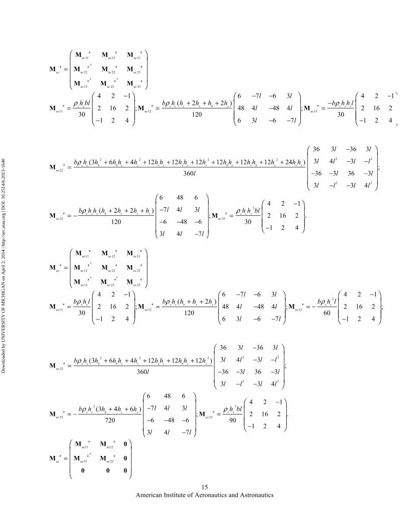
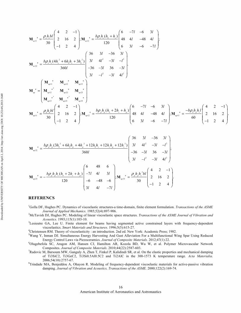
APPENDIX B FINITE ELEMENT MASS MATRIX This section presents the mass matrix developed in 3 but with corrected typos from their work.

22w w=⎛ ⎞⎜ ⎟⎜ ⎟⎜ ⎟⎝ ⎠

e e

0 0 0

M 0 M 0

0 0 0

2 2

22

2 2

156 22 54 13

22 4 13 3( )

54 13 156 22420

13 3 22 4

.b b c c v v s s p p

w

l l

l l l lbl h h h h h

l l

l l l l

ρ ρ ρ ρ ρ

−

−+ + + +=

−

− − −

⎛ ⎞⎜ ⎟⎜ ⎟⎜ ⎟⎜ ⎟⎝ ⎠

eM

11 12

12 22

ub ub

ub ub ub=

⎛ ⎞⎜ ⎟⎜ ⎟⎜ ⎟⎝ ⎠

T

e e

e e e

M M 0

M M M 0

0 0 0

2 23

11 12 22

2 2

36 3 36 34 2 1 0 0 0 0

3 4 32 16 2 ; 0 0 0 0 ;

36 3 36 330 3601 2 4 0 0 0 0

3 3 4

.b b b bub ub ub

l l

l l l lh bl b h

l ll

l l l l

ρ ρ

−−

− −= = =

− − −−

− −

⎛ ⎞⎛ ⎞ ⎛ ⎞ ⎜ ⎟⎜ ⎟ ⎜ ⎟ ⎜ ⎟⎜ ⎟ ⎜ ⎟ ⎜ ⎟⎜ ⎟ ⎜ ⎟⎝ ⎠ ⎝ ⎠ ⎜ ⎟⎝ ⎠

e e eM M M

Dow

nloa

ded

by U

NIV

ER

SIT

Y O

F M

ICH

IGA

N o

n A

pril

2, 2

014

| http

://ar

c.ai

aa.o

rg |

DO

I: 1

0.25

14/6

.201

3-16

40


15

11 12 13

12 22 23

13 23 33

uc uc uc

uc uc uc uc

uc uc uc

=

⎛ ⎞⎜ ⎟⎜ ⎟⎜ ⎟⎝ ⎠

T

T T

e e e

e e e e

e e e

M M M

M M M M

M M M

11 12 13

4 2 1 6 7 6 3 4 2 1( 2 2 )

2 16 2 ; 48 4 48 4 ; 2 16 230 120 30

1 2 4 6 3 6 7 1 2 4

.c c c c c v b s c c vuc uc uc

l lh bl b h h h h h b h h l

l l

l l

ρ ρ ρ− − − −

+ + + −= = − =

− − − −

⎛ ⎞ ⎛ ⎞ ⎛ ⎞⎜ ⎟ ⎜ ⎟ ⎜ ⎟⎜ ⎟ ⎜ ⎟ ⎜ ⎟⎜ ⎟ ⎜ ⎟ ⎜ ⎟⎝ ⎠ ⎝ ⎠ ⎝ ⎠

e e eM M M

2 22 2 2 2

22

2 2

23

36 3 36 3

3 4 3(3 6 4 12 12 12 12 12 12 24 );

36 3 36 3360

3 3 4

6 48 6

7 4 3( 2 2 )

6 48 6120

3 4 7

c c b b c c s c v c v b s v b s v suc

c c v b v s cuc

l l

l l l lb h h h h h h h h h h h h h h h h h

l ll

l l l l

l l lb h h h h h h

l l l

ρ

ρ

−

− −+ + + + + + + + +=

− − −

− −

−+ + += −

− − −

−

⎛ ⎞⎜ ⎟⎜ ⎟⎜ ⎟⎜ ⎟⎝ ⎠

⎛ ⎞⎜⎜⎜⎜⎝

e

e

M

M2

33

4 2 1

; 2 16 230

1 2 4

.c c vuc

h h blρ−

=

−

⎛ ⎞⎟⎜ ⎟⎟⎜ ⎟⎟ ⎜ ⎟⎝ ⎠⎟⎠

eM

11 12 13

12 22 23

13 23 33

uv uv uv

uv uv uv uv

uv uv uv

=

⎛ ⎞⎜ ⎟⎜ ⎟⎜ ⎟⎝ ⎠

T

T T

e e e

e e e e

e e e

M M M

M M M M

M M M

2

11 12 13

4 2 1 6 7 6 3 4 2 1( 2 )

2 16 2 ; 48 4 48 4 ; 2 16 2 ;30 120 60

1 2 4 6 3 6 7 1 2 4

v v v v b v s v vuv uv uv

l lb h l b h h h h b h l

l l

l l

ρ ρ ρ− − − −

+ += = − = −

− − − −

⎛ ⎞ ⎛ ⎞ ⎛ ⎞⎜ ⎟ ⎜ ⎟ ⎜ ⎟⎜ ⎟ ⎜ ⎟ ⎜ ⎟⎜ ⎟ ⎜ ⎟ ⎜ ⎟⎝ ⎠ ⎝ ⎠ ⎝ ⎠

e e eM M M

2 22 2 2

22

2 2

2 3

23 33

36 3 36 3

3 4 3(3 6 4 12 12 12 );

36 3 36 3360

3 3 4

6 48 64 2 1

7 4 3(3 4 6 ); 2 16 2

6 48 6720 90

3 4 7

v v b b v v s v b s suv

v v b v s v vuv uv

l l

l l l lb h h h h h h h h h h

l ll

l l l l

l l lb h h h h h bl

l l l

ρ

ρ ρ

−

− −+ + + + +=

− − −

− −

−−+ +

= − =− − −

−

⎛ ⎞⎜ ⎟⎜ ⎟⎜ ⎟⎜ ⎟⎝ ⎠

⎛ ⎞⎜ ⎟⎜ ⎟⎜ ⎟⎜ ⎟⎝ ⎠

e

e e

M

M M

1 2 4

.−

⎛ ⎞⎜ ⎟⎜ ⎟⎜ ⎟⎝ ⎠

11 12

12 22

us us

us us us=

⎛ ⎞⎜ ⎟⎜ ⎟⎜ ⎟⎝ ⎠

T

e e

e e e

M M 0

M M M 0

0 0 0

Dow

nloa

ded

by U

NIV

ER

SIT

Y O

F M

ICH

IGA

N o

n A

pril

2, 2

014

| http

://ar

c.ai

aa.o

rg |

DO

I: 1

0.25

14/6

.201

3-16

40


16

11 12

2 22 2

22

2 2

4 2 1 6 7 6 3( )

2 16 2 ; 48 4 48 4 ;30 120

1 2 4 6 3 6 7

36 3 36 3

3 4 3(4 6 3 )

36 3 36 3360

3 3 4

.

s s s s b sus us

s s s b s bus

l lh bl b h h h

l l

l l

l l

l l l lb h h h h h

l ll

l l l l

ρ ρ

ρ

− − −+

= = −

− − −

−

− −+ +=

− − −

− −

⎛ ⎞ ⎛ ⎞⎜ ⎟ ⎜ ⎟⎜ ⎟ ⎜ ⎟⎜ ⎟ ⎜ ⎟⎝ ⎠ ⎝ ⎠

⎛ ⎞⎜ ⎟⎜ ⎟⎜ ⎟⎜ ⎟⎝ ⎠

e e

e

M M

M

11 12 13

12 22 23

13 23 33

up up up

up up up up

up up up

=

⎛ ⎞⎜ ⎟⎜ ⎟⎜ ⎟⎝ ⎠

T

T T

e e e

e e e e

e e e

M M M

M M M M

M M M

11 12 13

4 2 1 6 7 6 3 4 2 1( 2 )

2 16 2 ; 48 4 48 4 ; 2 16 230 120 60

1 2 4 6 3 6 7 1 2 4

.p p b v p b p vb bup up up

l lb h h h h b h h lh bl

l l

l l

ρ ρρ− − − −

+ + −= = − =

− − − −

⎛ ⎞ ⎛ ⎞ ⎛ ⎞⎜ ⎟ ⎜ ⎟ ⎜ ⎟⎜ ⎟ ⎜ ⎟ ⎜ ⎟⎜ ⎟ ⎜ ⎟ ⎜ ⎟⎝ ⎠ ⎝ ⎠ ⎝ ⎠

e e eM M M

2 22 2 2

22

2 2

2

23 33

36 3 36 3

3 4 3(3 6 4 12 12 12 );

36 3 36 3360

3 3 4

6 48 64 2 1

7 4 3( 2 ); 2 16

6 48 6120 30

3 4 7

p p b b p p b v v p v

up

p p v b v p p p v

up up

l l

l l l lb h h h h h h h h h h

l ll

l l l l

l l lb h h h h h h h bl

l l l

ρ

ρ ρ

−

− −+ + + + +=

− − −

− −

−−+ +

= − =− − −

−

⎛ ⎞⎜ ⎟⎜ ⎟⎜ ⎟⎜ ⎟⎝ ⎠

⎛ ⎞⎜ ⎟⎜ ⎟⎜ ⎟⎜ ⎟⎝ ⎠

e

e e

M

M M 2

1 2 4

.−

⎛ ⎞⎜ ⎟⎜ ⎟⎜ ⎟⎝ ⎠

REFERENCS

1Golla DF, Hughes PC. Dynamics of viscoelastic structures-a time-domain, finite element formulation. Transactions of the ASME Journal of Applied Mechanics. 1985;52(4):897-906.

2McTavish DJ, Hughes PC. Modeling of linear viscoelastic space structures. Transactions of the ASME Journal of Vibration and Acoustics. 1993;115(1):103-10.

3Lesieutre GA, Lee U. Finite element for beams having segmented active constrained layers with frequency-dependent viscoelastics. Smart Materials and Structures. 1996;5(5):615-27.

4Christensen RM. Theory of viscoelasticity : an introduction. 2nd ed. New York: Academic Press; 1982. 5Wang Y, Inman DJ. Simultaneous Energy Harvesting And Gust Alleviation For a Multifunctional Wing Spar Using Reduced

Energy Control Laws via Piezoceramics. Journal of Composite Materials. 2012;47(1):22. 6Olugebefola SC, Aragon AM, Hansen CJ, Hamilton AR, Kozola BD, Wu W, et al. Polymer Microvascular Network

Composites. Journal of Composite Materials. 2010;44(22):2587-603. 7Radovic M, Barsoum MW, Ganguly A, Zhen T, Finkel P, Kalidindi SR, et al. On the elastic properties and mechanical damping

of Ti3SiC2, Ti3GeC2, Ti3Si0.5Al0.5C2 and Ti2AlC in the 300-1573 K temperature range. Acta Materialia. 2006;54(10):2757-67.

8Trindade MA, Benjeddou A, Ohayon R. Modeling of frequency-dependent viscoelastic materials for active-passive vibration damping. Journal of Vibration and Acoustics, Transactions of the ASME. 2000;122(2):169-74.

Dow

nloa

ded

by U

NIV

ER

SIT

Y O

F M

ICH

IGA

N o

n A

pril

2, 2

014

| http

://ar

c.ai

aa.o

rg |

DO

I: 1

0.25

14/6

.201

3-16

40

Documents

Experimental and Finite Element Analysis for a