Embed Size (px)
Citation preview

Mississippi State University Mississippi State University
Scholars Junction Scholars Junction
Theses and Dissertations Theses and Dissertations
8-2-2003
Experimental Measurement and Finite Element Simulation of Experimental Measurement and Finite Element Simulation of
Springback in Stamping Aluminum Alloy Sheets for Auto-Body Springback in Stamping Aluminum Alloy Sheets for Auto-Body
Panel Application Panel Application
Crisbon Delfina Joseph
Follow this and additional works at: https://scholarsjunction.msstate.edu/td
Recommended Citation Recommended Citation Joseph, Crisbon Delfina, "Experimental Measurement and Finite Element Simulation of Springback in Stamping Aluminum Alloy Sheets for Auto-Body Panel Application" (2003). Theses and Dissertations. 2146. https://scholarsjunction.msstate.edu/td/2146
This Graduate Thesis - Open Access is brought to you for free and open access by the Theses and Dissertations at Scholars Junction. It has been accepted for inclusion in Theses and Dissertations by an authorized administrator of Scholars Junction. For more information, please contact [email protected].

EXPERIMENTAL MEASUREMENT AND FINITE ELEMENT SIMULATION OF
SPRINGBACK IN STAMPING ALUMINUM ALLOY SHEETS FOR
AUTO-BODY PANEL APPLICATION
By
Crisbon Delfina Joseph
A Thesis Submitted to the Faculty of Mississippi State University
in Partial Fulfillment of the Requirements for the Degree of Master of Science
in Mechanical Engineering in the Department of Mechanical Engineering
Mississippi State, Mississippi
August 2003
EXPERIMENTAL MEASUREMENT AND FINITE ELEMENT SIMULATION OF
SPRINGBACK IN STAMPING ALUMINUM ALLOY SHEETS FOR
AUTO-BODY PANEL APPLICATION
By
Crisbon Delfina Joseph
Approved:
_________________________________ _________________________________ Judy A. Schneider Steven R. Daniewicz Assistant Professor of Mechanical Associate Professor of Mechanical Engineering (Director of Thesis) Engineering (Committee Member) _________________________________ _________________________________ John T. Berry Rogelio Luck Professor of Mechanical Engineering Graduate Coordinator of the Department (Committee Member) of Mechanical Engineering
_________________________________ A. Wayne Bennett Dean of the College Engineering

Name: Crisbon Delfina Joseph Date of Degree: August 2, 2003 Institution: Mississippi State University Major Field: Mechanical Engineering Major Professor: Dr. Judy A. Schneider Title of Study: EXPERIMENTAL MEASUREMENT AND FINITE ELEMENT
SIMULATION OF SPRINGBACK IN STAMPING ALUMINUM ALLOY SHEETS FOR AUTO-BODY PANEL APPLICATION
Pages in Study: 83 Candidate for Degree of Master of Science
Use of weight-saving materials to produce lightweight components with enhanced
dimensional control is important to the automotive industry. This has increased the need
to understand the material behavior with respect to the forming process at the
microstructural level. A test matrix was developed based on the orthogonal array of
Taguchi design of experiment (DOE) approach. Experiments were conducted for the V-
bending process using 6022-T4 AA to study the variation of springback due to both
process and material parameters such as bend radius, sheet thickness, grain size, plastic
anisotropy, heat treatment, punching speeds, and time. The design of experiments was
used to evaluate the predominate parameters for a specific lot of sheet metal. It was
observed that bend radius had greatest effect on springback. Next, finite element
simulation of springback using ANSYS implicit code was conducted to explore the limits
regarding process control by boundary values versus material parameters. 2-D finite
element modeling was considered in the springback simulations. A multilinear isotropic

material model was used where the true stress-strain material description was input in
discrete form. Experimental results compare well with the simulated predictions. It was
found that the microstructure of the material used in this study was processed for sheet
metal forming process.

ii
DEDICATION
To my family and friends

iii
ACKNOWLEDGEMENTS
First of all, I would like to express my sincere gratitude to my major advisor Dr.
Judy A. Schneider for her constant support and motivation throughout the entire period of
this research. Dr. Schneider is the most important reason for my success in publication
and presentation of papers in various conferences. I always revere her patience and
encouragement. I would also like to thank my committee members Dr. Steven R.
Daniewicz and Dr. John T. Berry for their suggestions and guidance provided in the
realization of this research. Mr. Grant Harlow is greatly appreciated for designing and
fabricating the tooling used for testing in this research. Acknowledgement is due to
ALCOA for providing us with the sheet metal that was studied in this research. Finally, I
would like to thank CAVS (Center of Advanced Vehicular Systems), MSU for funding
this research in conjunction with Nissan.
iv
TABLE OF CONTENTS
Page
DEDICATION........................................................................................................... ii
ACKNOWLEDGEMENTS....................................................................................... iii
LIST OF TABLES..................................................................................................... vii
LIST OF FIGURES ................................................................................................... ix
NOMENCLATURE .................................................................................................. xi
CHAPTER
I. INTRODUCTION.......................................................................................... 1
1-1 Research Objective................................................................................ 1 1-2 Project Overview................................................................................... 2
II. BACKGROUND ........................................................................................... 4
2-1 Sheet Metal Forming Process................................................................. 4 2-2 V-Bending Process ................................................................................. 6 2-3 Springback.............................................................................................. 7
III. EXPERIMENTAL DESCRIPTION............................................................. 9
3-1 Material Characterization ....................................................................... 9 3-1-1 Microstructure.............................................................................. 10 3-1-2 Heat Treatment / Hardness .......................................................... 11 3-1-3 Tensile Testing............................................................................. 12
3-2 Design of Experiments ........................................................................... 14 3-2-1 Taguchi Methodology.................................................................. 14 3-2-2 Taguchi Matrix ............................................................................ 15

v
CHAPTER Page
3-3 V-Bend Fixture....................................................................................... 17
IV.FINITE ELEMENT ANALYSIS ......................................................................... 19
4-1 Literature Review ................................................................................. 19 4-1-1 Finite Element Codes.................................................................. 20 4-1-2 Summary of Elements used in SMF Simulation ........................ 22 4-1-3 Material Behavior....................................................................... 23 4-1-4 Yield Criterion............................................................................ 24 4-1-5 Constitutive Models ................................................................... 28
4-2 Sheet Metal Forming Simulation......................................................... 32 4-2-1 Sheet Metal Forming Codes ...................................................... 32 4-2-2 Convergence Criteria.................................................................. 33
4-3 Springback Simulation ........................................................................ 34 4-3-2 V-Bend Simulation Approach .................................................... 36
V. RESULTS ....................................................................................................... 39
5-1 Taguchi DOE Test Results ................................................................... 39 5-1-1 ANOVA (Analysis of Variance)............................................... 40 5-1-2 S/N ANOVA (Signal to Noise ANOVA) ................................. 42
5-2 Simulation Test Cases .......................................................................... 43 5-2-1 V-Bend Simulation Results....................................................... 44
VI. DISCUSSION................................................................................................. 47
6-1 Taguchi Experimental Results.............................................................. 47 6-1-1 Effect of Bend Radius ............................................................... 48 6-1-2 Effect of Other Factors.............................................................. 50 6-1-3 Other Defects Observed............................................................ 51
6-2 Finite Element Simulation.................................................................... 51 6-3 Comparison of Experimental and Simulation Results.......................... 51
6-4 Orientation Imaging Microscopy ......................................................... 52
VII. CONCLUSIONS............................................................................................ 54

vi
CHAPTER Page VIII. RECOMMENDED FOLLOW-ON STUDIES.............................................. 55 REFERENCES .......................................................................................................... 56 APPENDIX
A UNIAXIAL TENSION TEST RESULTS..................................................... 64
B V-BEND TEST PROCEDURE ..................................................................... 69
C TAGUCHI ANALYSIS DESCRIPTION...................................................... 72
D ANSYS INPUT FILE MAC.DAT .................................................................. 82

vii
LIST OF TABLES
TABLE Page
3-1 Registered Composition (in wt.%) of Aluminum Alloy 6022 per Aluminum Association Inc. ..............................................................................................9
3-2 Polishing Procedure for 6022-T4 AA....................................................................10
3-3 Rockwell B Hardness Values at Various Temperatures ........................................12
3-4 Mechanical Properties of 6022-T4 AA Tested in Uniaxial Tension at Different Directions......................................................................................................14
3-5 (a) Factor and Level Descriptions..........................................................................16
(b) L18 Test Matrix.................................................................................................17
4-1 Implicit vs. Explicit codes .....................................................................................21
4-2 Elements used in SMF Simulation.........................................................................23
4-3 Various Yield Criteria Reported in Literature .......................................................27
4-4 (a) Non-Linear Inelastic Models ............................................................................30
(b) Material Models Requiring Equations of State................................................31
4-5 Commercially Available Finite Element Codes for SMF Simulation....................33
5-1 The L18 Test Matrix and Recorded Springback Angles .........................................40
5-2 Initial ANOVA for Springback Measurement .......................................................41
5-3 Pooled ANOVA Table……………………………………………………………41 5-4 Initial S/N ANOVA................................................................................................43
5-5 Pooled S/N ANOVA Table ....................................................................................43

viii
TABLE Page
5-6 Finite Element Simulation Test Matrix ..................................................................44
5-7 V-Bend Simulation Results ....................................................................................45
C-1 Totals Table for Analysis of Variance...................................................................74
C-2 Signal to Noise Ratios for the V-Bend Experiments .............................................78

ix
LIST OF FIGURES
FIGURE Page
1-1 V-Bend Project Overview........................................................................................2
1-2 Design Parameters that Effect Springback ..............................................................3
2-1 Bending of Sheet Metal ...........................................................................................6
2-2 V-Bending Process...................................................................................................7
2-3 Springback Phenomenon .........................................................................................7
3-1 As-Received Microstructure of 6022-T4 AA ........................................................10
3-2 Heat Treatment Study of 6022-T4 AA ..................................................................11
3-3 Uniaxial Tensile Testing........................................................................................12
3-4 True Stress-Strain Plots for 6022-T4 AA in Three Directions to the Rolling Plane..............................................................................................................13
3-5 (a) V-Bend fixture installed on Model 5800 Instron machine, (b) V-
Bend Process.................................................................................................18
5-1 V-Bend Model with Boundary Conditions and Mesh ...........................................44
5-2 Simulated Result for Bend Radius 3mm................................................................45
5-3 Simulated Result for Bend Radius 5mm................................................................45
5-4 Simulated Result for Bend Radius 9.5mm.............................................................45
6-1 V-Bends at Different Bend Radii ...........................................................................49
6-2 Variation of Springback Angle with Respect to Different Bend Radii ..................49
6-3 Comparison of Experimental and Simulation Results............................................51
6-4 OIM Images for 6022-T4 AA Material as per INCA Inc.………………………. 53

x
FIGURE Page
A-1 Stress Strain Plot at Different Speeds When Tested 0 Degrees to Rolling Direction .......................................................................................................65
A-2 Stress Strain Plot at Different Speeds When Tested 45 Degrees to Rolling Direction .......................................................................................................66
A-3 Stress Strain Plot at Different Speeds When Tested 90 Degrees to Rolling Direction .......................................................................................................66
A-4 Mechanical Properties of 6022-T4 AA…………………………………………..68

xi
NOMENCLATURE
)( ijF σ = Yield Function
321 ,, σσσ = Principal Stresses
321 ,, nnn = Principal Directions
σ = Flow Stress
E = Young’s Modulus ε = Strain
k = Material Constant
n = Strain Hardening Exponent
DOF = Degrees of Freedom
S = Sum of Squares
V = Variance Between the Individual Control Factor Effects
Ve = Variance in the Experimental Data Due to Random Experimental Error
P% = Percentage Contribution
S’ = Pure Sum of Squares
ST = Sum of Squares for Total
NS/ = Overall Mean Signal to Noise Ratio
STBNS / = Smaller the Better Type S/N Ratio
y = Mean
GTSS = Grand Total Sum of Squares

1
CHAPTER I
INTRODUCTION 1-1 Research Objective
The objective of this research is to study the sheet metal forming/stamping aspects
of automotive manufacture, specifically the relative contribution of material and process
parameters on the formability of lightweight auto-body materials. This project was
motivated because the production of lightweight car exteriors with enhanced repeatable
dimensional tolerances is important to the automotive industry. Many of these parts are
formed using sheet metal stamping. The use of aluminum alloy sheets in the manufacture
of auto-body panels has increased fourfold in the automotive industry because of its high
strength, low density and corrosion resistance. But one of the major concerns of stamping
lightweight aluminum alloys is springback. Hence, to be cost effective, accurate
predictions must be made of its formability. The automotive industry places rigid
constraints on final shape and dimensional tolerances. Compensating for springback
becomes critical in this highly automated environment.
Springback or elastic recovery relates to the change in shape between the fully
loaded and unloaded configurations the material encounters during a stamping operation.
This results in the formed component being out of tolerance and can create major
problems in the assembly or installation.

2
Accurate springback prediction is imperative for robust design of tooling; thereby
saving costs and die try-out times. The effect of the various process and material
parameters on spring-back and spring-in are examined in this research. A 090 V-Bend
process was selected for this study. The sheet material used is 6022-T4 aluminum alloy
developed by ALCOA in the early 90’s.
1-2 Project Overview
Figure 1-1 V-Bend Project Objective
This thesis is comprised of two parts as shown in Figure 1-1. The first part
involves the experimental measurement of springback, and the second part deals with

3
springback simulation. Previous investigations [1-12] have studied the effect of certain
process or material parameters on springback. This study will evaluate processing
parameters in addition to material parameters in relation to their overall contribution to
springback. In the first part, experiments were designed using the Taguchi design of
experiments (DOE) methodology [13] to include the various process and material
parameters that effect springback as illustrated in Figure1-2. V-bend fixtures were
designed and fabricated and the test matrix was set up. Results were recorded and
analyzed, and the relative significance of the various factors that have been reported to
effect springback was determined [14]. Based on the experimental results, appropriate
material models were used to simulate the process. The literature concerning factors
affecting springback is split between processing parameters and material parameters.
Once a relative ranking of process parameters and material parameters for a given lot of
material is obtained, the process can be modeled using FE.
Figure1-2 Design Parameters that Effect Springback
4
CHAPTER II
BACKGROUND 2-1 Sheet Metal Forming Process
Sheet metal forming (SMF) is one of the most common metal manufacturing
process used. Its applications are wide in aircraft components, automobile components
etc. The characteristics of sheet metal forming processes are: (1) the work piece is a sheet
or a part fabricated from a sheet (2) the surfaces of the deforming material and of the
tools are in contact (3) the deformation usually causes significant changes in shape, but
not in cross-section (sheet thickness and surface characteristics), of the sheet (4) in some
cases, the magnitude of permanent plastic and recoverable elastic deformation is
comparable, therefore elastic recovery or springback may be significant.
The technical-economic advantages of SMF are that it is a highly efficient process
that can be used to produce complex parts. It can produce parts with high degree of
dimensional accuracy and increased mechanical properties along with a good surface
finish. But the limitation is that the deformation imposed in SMF process is complicated.
Stamping is one type of sheet metal forming process, which is widely used in
automotive industries. The popularity of stamping is mainly due to its high productivity,
relatively low assembly costs and the ability to offer high strength and lightweight
products [15].

5
In general, the deformation of sheet materials in the stamping process is classified
by four types of deformation modes; i.e., bending, deep drawing, stretching and stretch
flanging. Since this project deals with the bending process, this study will be focused on
the bending operation.
Bending is the plastic deformation of metals about a linear axis called the bending
axis with little or no change in the surface area. Bending types of forming operations
have been used widely in sheet metal forming industries to produce structural stamping
parts such as braces, brackets, supports, hinges, angles, frames, channel and other non-
symmetrical sheet metal parts [16].
One of the important characteristics noticed during the bending operation is that
the tensile stress decreases toward the center of the sheet thickness and becomes zero at
the neutral axis whereas the compressive stress increases from the neutral axis toward the
inside of the bend as shown in Figure 2-1. Even with large plastic deformation in
bending, the center region (elastic metal band or zone) of the sheet remains elastic and so
on unloading elastic recovery occurs [15].

6
Figure 2-1 Bending of Sheet Metal
2-2 V-Bending Process
Figure 2-2 illustrates the V-bending process. Sheet metal is placed over the die
and bent as the punch descends into the die. The V-die bending process falls into two
categories, namely air bending and bottom bending. This study is limited to bottom
bending, in which the punch fully sets in the die. The first diagram shows the loading
process and the second one shows the forming of the V-bend. Upon unloading (third
diagram) springback or spring-in (negative springback) is observed depending on the
process and material parameters used, this context is explained in the later chapters.
Plastic deformation
Elastic zone
Tensile stresses
Compressive stresses
Springback forces
Neutral axis

7
Figure 2-2 V-Bending Process
2-3 Springback
Springback or elastic recovery refers to the shape discrepancy between the fully
loaded and unloaded configurations. The stress strain plot shown in Figure 2-3 illustrates
the springback phenomenon. Upon unloading in a stamping process there is elastic
recovery, which is the release of the elastic strains and the redistribution of the residual
stresses through the thickness direction, thus producing springback.
Figure 2-3 Springback Phenomenon
Spring-in
Springback
Punch
Sample
Die
Plastic deformation
Elastic recovery
Stress
Strain
UnloadLoad

8
Springback causes changes in shape and dimensions that can create major
problems in the assembly; hence springback prediction is an important issue in sheet
metal forming industry. Many factors could affect springback in the process, such as
material variations in mechanical properties, sheet thickness, tooling geometry (including
die radius and the gap between the die and the punch), processing parameters and
lubricant condition [16]. Various investigations [1-12] of springback prediction show that
process parameters such as bend radius, die gap and punching speeds, and material
properties such as sheet thickness, flow stress, texture and grain size have considerable
influence on springback. Many of the factors affecting springback are also manifested in
the minimum bending radius or bendability limit in addition to the surface or edge
condition of the sheet [17]. Hisashi’s [18] research showed the effect of increasing the die
profile radius as the material strength increases. Larger springback has been correlated
with an increase in normal anisotropy and decrease in strain hardening exponent
[3,12,19,20].

9
CHAPTER III
EXPERIMENTAL DESCRIPTION 3-1 Material Characterization
6022- T4 aluminum developed in early 1990’s by ALCOA, is becoming popular
in automotive industry, it is the material that was used in this project. This aluminum
alloy is a precipitation-strengthened alloy with major alloying elements Mg and Si. It is
intended for automotive body sheet applications. The T-4 processing includes a high-
temperature solution heat treatment, a quench, and then natural aging to a
microstructurally stable condition. The chemistry and material properties of the material
received from ALCOA are summarized in Table 3-1.
Table 3-1 Registered Composition (in wt.%) of Aluminum Alloy 6022 per Aluminum
Association Inc. (Note: single numbers refer to the maximum values)
Property Value Composition Si 0.8-1.5, Mg 0.45-0.70, Fe 0.05-0.20, Mn 0.02-
0.10, Cu 0.01-0.11, Ti 0.15, Cr 0.10, Zn 0.25 Young’s Modulus 69 GPa UTS 236-237 MPa Yield Strength 125-126 MPa Elongation 27.5%
10
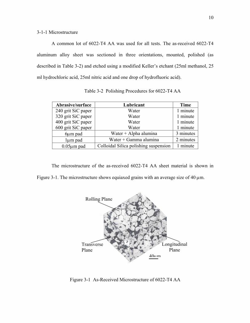
3-1-1 Microstructure
A common lot of 6022-T4 AA was used for all tests. The as-received 6022-T4
aluminum alloy sheet was sectioned in three orientations, mounted, polished (as
described in Table 3-2) and etched using a modified Keller’s etchant (25ml methanol, 25
ml hydrochloric acid, 25ml nitric acid and one drop of hydrofluoric acid).
Table 3-2 Polishing Procedures for 6022-T4 AA
Abrasive/surface Lubricant Time 240 grit SiC paper 320 grit SiC paper 400 grit SiC paper 600 grit SiC paper
Water Water Water Water
1 minute 1 minute 1 minute 1 minute
6µm pad Water + Alpha alumina 3 minutes 1µm pad Water + Gamma alumina 2 minutes
0.05µm pad Colloidal Silica polishing suspension 1 minute
The microstructure of the as-received 6022-T4 AA sheet material is shown in
Figure 3-1. The microstructure shows equiaxed grains with an average size of 40 µm.
Figure 3-1 As-Received Microstructure of 6022-T4 AA
Rolling Plane
Transverse Plane
Longitudinal Plane
40µm

11
3-1-2 Heat Treatment / Hardness
A comprehensive heat treatment study was conducted to increase the grain size of
the material without changing its hardness. This was done to vary the grain size for the
test matrix. Negligible grain growth was observed in Al 6022-T4 below 560° C as shown
in Figure 3-2. The software Scion Image [21] was used to measure the diameter of the
grains. The dark areas in the figure constitute the second phase Mg2Si particles. The grain
sizes of 125 µm and 185 µm were obtained by heat-treating the material at 560° C for
4hrs and 24 hrs respectively.
Figure 3-2 Heat Treatment Study of 6022-T4 AA
12
Rockwell B hardness tests indicated negligible change in the hardness of the
material due to heat treatment as illustrated in Table 3-3.
Table 3-3 Rockwell B Hardness Values at Various Temperatures.
Test Points 1 2 3 4 Average Room Temp. 64.5 68.0 71.0 68.5 68.0 +/-4.0 560 C, 4hrs. 67.0 71.5 68.0 72.5 69.8 +/-4.0 560 C, 24hrs. 63.0 67.0 70.5 77.5 69.5 +/-7.0
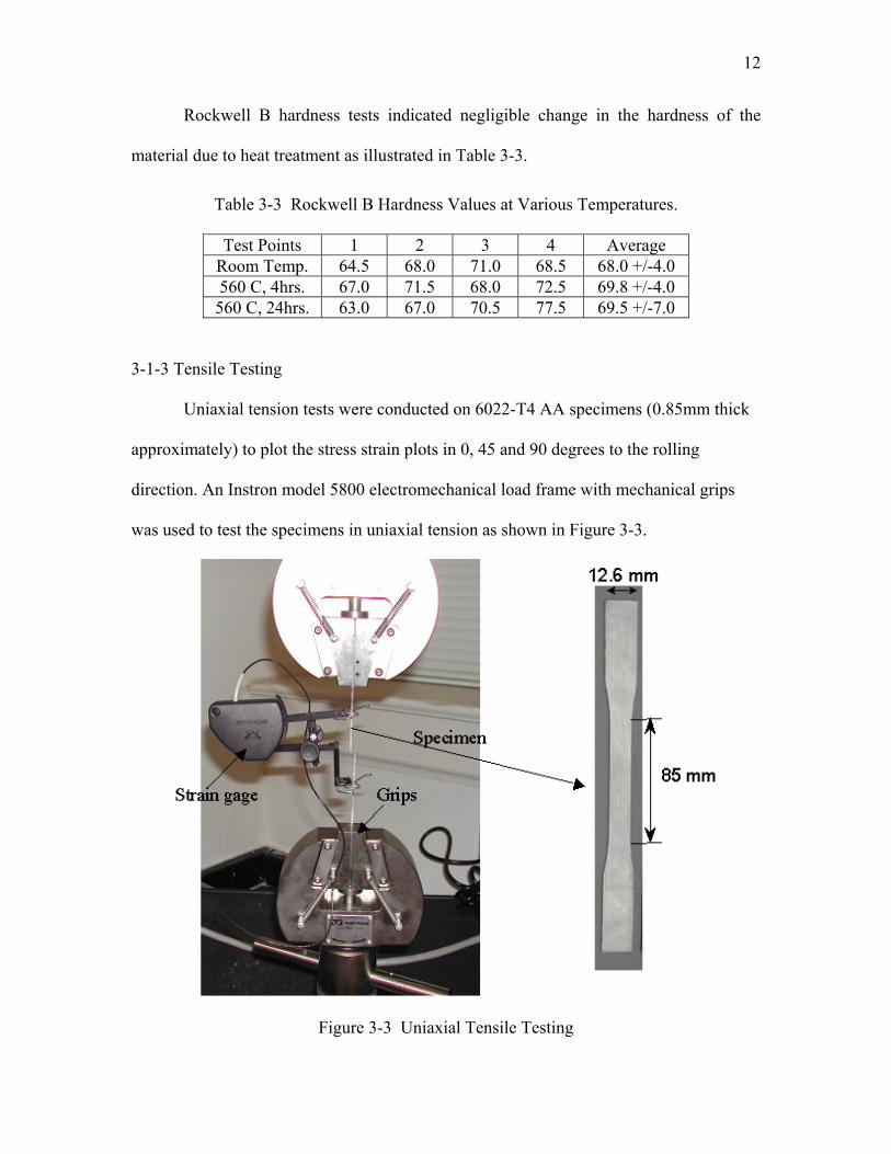
3-1-3 Tensile Testing
Uniaxial tension tests were conducted on 6022-T4 AA specimens (0.85mm thick
approximately) to plot the stress strain plots in 0, 45 and 90 degrees to the rolling
direction. An Instron model 5800 electromechanical load frame with mechanical grips
was used to test the specimens in uniaxial tension as shown in Figure 3-3.
Figure 3-3 Uniaxial Tensile Testing

13
Three repeats at each orientation was conducted. Also, the tests were run at
different speeds i.e. at minimum and maximum speed of the Instron machine (5.1mm/min
and 510mm/min), but it was found that the material properties were rate independent as
seen in Appendix A. The following Figure 3-4 shows the true stress-strain plots of 6022-
T4 AA in three different directions.
6022-T4 AA
0
50
100
150
200
250
300
350
400
0 0.05 0.1 0.15 0.2 0.25
True Strain (mm/mm)
True
Str
ess
(MPa
)
0 degrees45 degrees90 degrees
Figure 3-4 True Stress-Strain Plots for 6022-T4 AA in Three Directions to the Rolling
Plane
This data will be used in the simulations to observe the effect of material behavior
(texture) on springback. The other data in three directions to rolling direction (RD) are
listed in Table 3-4 and the respective plots are illustrated in Appendix A.
Grain size = 40µm

14
Table 3-4 Mechanical Properties of 6022-T4 AA Tested in Uniaxial Tension at
Different Directions.
Property 0 degrees to RD
45 degrees to RD
90 degrees to RD
Young’s modulus 69 GPa 69 GPa 69 GPa Yield Strength (0.2% offset) 170 MPa 160 MPa 163 MPa
Ultimate Tensile Strength 285 MPa 272 MPa 273 MPa % Elongation to Failure 20.27 22.63 21.52
Toughness 46.21 MPa 45.48 MPa 46.16 MPa Resilience (Work) 0.51 MPa 0.4 MPa 0.489 MPa
r value [45] 0.7 0.48 0.59
3-2 Design of Experiments
3-2-1 Taguchi Methodology
The Taguchi design of experiments method was used in this project to evaluate
the relative contribution of process and material parameters on springback in V-die
bending.
According to Taguchi, quality characteristic is a parameter whose variation has a
critical effect on product quality, e.g., weight, cost, target thickness, strength, material
properties, etc. The Taguchi quality strategy is to improve quality in the product design
stage by: (1) making the design less sensitive towards influence of uncontrollable factors
and (2) Optimizing the product design.
Designing an experiment:
Taguchi method uses a special set of arrays called orthogonal arrays. These
standard arrays stipulate the way of conducting the minimal number of experiments,
which could give the full information of all the factors that affect the performance
parameters [13].

15
3-2-2 Taguchi Matrix
Experiments were designed to study the parameters that effect springback. Three
levels of sheet thickness were chosen to represent variations in the as-received sheet.
Bending the sheet metal at three different directions, parallel, perpendicular and forty-
five degrees to the rolling direction, was the boundary condition used to evaluate the
contribution of planar anisotropy on springback.
Zhang et al [20] have shown that forming speed has a great effect on springback
behavior of the formed part. The maximum tool velocity of the Instron model 5800 load
frame used for V-Bending is 8.5 mm/s; hence, the punching speeds are varied between
0.085mm/s and 8.5mm/s. Carden et al. [23] have speculated that for 6022-T4 aluminum,
the springback angles continued to increase for periods up to several months after sheet
metal forming. Hence, shelf life and dwell time were included in the test matrix.
Experimental investigations [4,24,25] and analytical calculations [12,26] showed that
when the ratio of the die gap to sheet thickness is slightly greater than one, the effect of
die gap on springback is greatest. For this study the die gap was set to be equal to the
sheet thickness, to eliminate the effect of die gap.
Carden et al [23] showed that friction in normal industrial ranges (i.e., well
lubricated to dry conditions) has no measurable effect on springback, although very low
friction conditions increase springback for 6022-T4. In this study, lubrication was not
taken into consideration. A common tool radius of 9.5mm is referenced for the
automotive industry [27]. For this study, three bending radii were selected, 3, 5, and 9.5
mm.

16
The following Tables 3-5a and 3-5b show the Taguchi test matrix for the tests to
be performed on prediction of springback during V-bending process. To design
experimental matrix for seven factors with three levels, the L18 orthogonal array was most
applicable. The L18 array requires the minimum number of tests (18) to investigate the
factor effect on springback. In this study only the individual effect of each factor on
springback was investigated. The L18 is not structured to study interactions.
Table 3-5a Factor and Level Descriptions
Factor Factor Description Level 1 Level 2 Level 3 A Bend Radius 3mm 5mm 9.5mm B Sheet Thickness 0.84mm 0.86mm 0.89mm C Grain size 40 µm 125 µm 185 µm D Rolling Direction Parallel Perpendicular 45 degrees E Punching speeds 0.085 mm/sec 0.85 mm/s 8.5 mm/s F Shelf life None 15 days 2 months G Dwell Time None 30 min 1 hour e Error N/A N/A N/A

17
Table 3-5b L18 Test Matrix
Factors Run # e A B C D E F G 1 1 1 1 1 1 1 1 1 2 1 1 2 2 2 2 2 2 3 1 1 3 3 3 3 3 3 4 1 2 1 1 2 2 3 3 5 1 2 2 2 3 3 1 1 6 1 2 3 3 1 1 2 2 7 1 3 1 2 1 3 2 3 8 1 3 2 3 2 1 3 1 9 1 3 3 1 3 2 1 2 10 2 1 1 3 3 2 2 1 11 2 1 2 1 1 3 3 2 12 2 1 3 2 2 1 1 3 13 2 2 1 2 3 1 3 2 14 2 2 2 3 1 2 1 3 15 2 2 3 1 2 3 2 1 16 2 3 1 3 2 3 1 2 17 2 3 2 1 3 1 2 3 18 2 3 3 2 1 2 3 1
3-3 V-Bend Fixture
A V-bend fixture was designed and built to install on a Model 5800 Instron EM
load frame as shown in Figures 3-5a and 3-5b. The description of the data sheet to record
data and also the procedure for conducting the v-bend test are explained in Appendix B.
The experiments were performed using the bend fixture. The dimensions of the sheet
metal specimens used in the V-bend test are 56mm length and 30.5mm width. The
sample is not restrained during the bending process. The two linear ball bearing/bushing
assemblies as shown in the figure guarantee accurate punch guidance.

18
Figure 3-5a V-Bend fixture installed on Model 5800 Instron machine
Figure 3-5b V-Bend Process
Bearing guides
sample
Inserts for varying punch radii
Fixture mounted to
compression platens

19
CHAPTER IV
FINITE ELEMENT ANALYSIS
4-1 Literature Review
The finite element method, a powerful numerical technique, has been applied in
the past years to a wide range of engineering problems. Although much FE analysis is
used to verify the structural integrity of designs, more recently FE has been used to model
fabrication processes. When modeling fabrication processes that involve deformation,
such as SMF, the deformation process must be evaluated in terms of stresses and strain
states in the body under deformation including contact issues. The major advantage of
this method is its applicability to a wide class of boundary value problems with little
restriction on work piece geometry.
The three basic requirements for the successful commercial application of
numerical simulation are [28]: (1) simplicity of application (2) accuracy and (3)
computing efficiency. The characteristic features of the finite element method are [29]:
The domain of the problem is represented by a collection of simple sub domains, called
finite elements. The collection of finite elements is called the finite element mesh. Over
each finite element, the physical process is approximated by functions of desired type
(polynomials or otherwise), and algebraic equations relating physical quantities at
selective points, called nodes, of the element are developed.

20
The use of finite element analysis is beneficial in the design of tooling in sheet
metal forming operations because it is more cost effective than trial and error. The prime
objective of an analysis is to assist in the design of the product by: (1) predicting the
material deformation and (2) predicting the forces and stresses necessary to execute the
forming operation.
4-1-1 Finite Element Codes:
Implicit vs Explicit Codes
Implicit code solves for equilibrium at the every time step (t+∆t). Depending
upon the procedure chosen, each iteration requires the formation and solution of the
linear system of equations. Explicit method solves for equilibrium at time t by direct
time integration. This explicit procedure is conditionally stable since iterative procedure
is not implemented to reach equilibrium and also ∆t is limited by natural time. The Table
4-1 summarizes the difference in implicit and explicit codes.
21
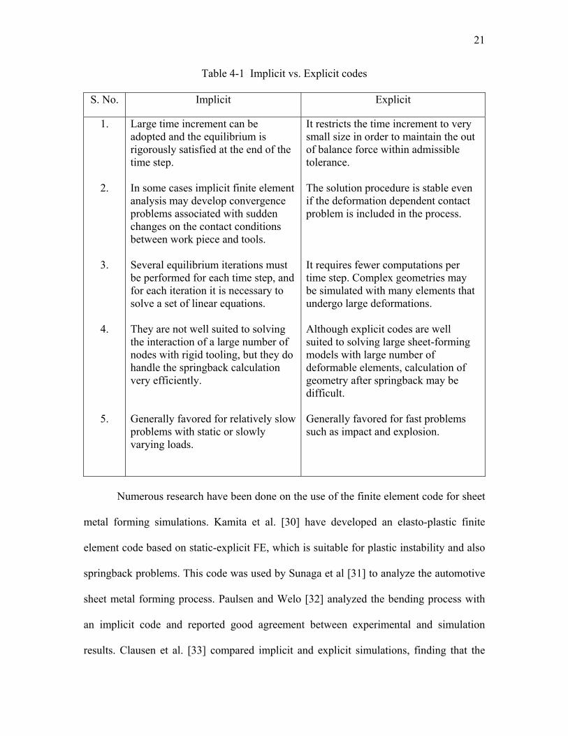
Table 4-1 Implicit vs. Explicit codes
S. No. Implicit Explicit
1.
2.
3.
4.
5.
Large time increment can be adopted and the equilibrium is rigorously satisfied at the end of the time step. In some cases implicit finite element analysis may develop convergence problems associated with sudden changes on the contact conditions between work piece and tools. Several equilibrium iterations must be performed for each time step, and for each iteration it is necessary to solve a set of linear equations. They are not well suited to solving the interaction of a large number of nodes with rigid tooling, but they do handle the springback calculation very efficiently. Generally favored for relatively slow problems with static or slowly varying loads.
It restricts the time increment to very small size in order to maintain the out of balance force within admissible tolerance. The solution procedure is stable even if the deformation dependent contact problem is included in the process. It requires fewer computations per time step. Complex geometries may be simulated with many elements that undergo large deformations. Although explicit codes are well suited to solving large sheet-forming models with large number of deformable elements, calculation of geometry after springback may be difficult. Generally favored for fast problems such as impact and explosion.
Numerous research have been done on the use of the finite element code for sheet
metal forming simulations. Kamita et al. [30] have developed an elasto-plastic finite
element code based on static-explicit FE, which is suitable for plastic instability and also
springback problems. This code was used by Sunaga et al [31] to analyze the automotive
sheet metal forming process. Paulsen and Welo [32] analyzed the bending process with
an implicit code and reported good agreement between experimental and simulation
results. Clausen et al. [33] compared implicit and explicit simulations, finding that the

22
response differences were almost negligible. Investigations have shown that explicit
method is well suited for solving large sheet forming models, and implicit codes handle
the springback calculation very efficiently. Hence, recently researchers have adopted a
new method of coupling the implicit and explicit methods to solve complex sheet metal
forming processes would save design effort and production time. Narasimhan et al. [34]
have used ANSYS/LS-DYNA explicit coupled with ANSYS implicit for springback
simulation. Finn et al. [35] combined the commercial codes LS-DYNA3D and NIKE3D
for prediction of springback in automotive body panels. Taylor et al. [36] discussed the
numerical solution of sheet-metal forming applications using the ABAQUS general-
purpose implicit and explicit finite-element modules.
4-1-2 Summary of Elements used in SMF Simulation
FEA of the sheet metal forming problem usually adopts one of three analysis
methods based on the membrane, shell and continuum element [37]. The Table 4-2
summarizes the elements used in finite element method for sheet metal forming
simulation.

23
Table 4-2 Elements used in SMF Simulation
Element Specialty Limitation
Membrane Computational efficiency and better convergence in contact analysis than the shell or continuum element [37]
It does not consider bending effect and has to tolerate inaccuracy in the bending dominant problems.
Shell Can capture the combination of stretching and bending as opposed
to membrane elements. Use of shell element gives more number of degrees of freedom to capture
accurate stress distribution including in- plane and out-plane deformation.
It takes a substantial amount of computational time and computer space for its 3-D calculation with
integration in the thickness direction.
Continuum Are used where fully 3-D theory is needed to describe the deformation process. They can handle through-
thickness compressive straining whereas shell elements cannot.
More elements are needed to describe the shell-type structures, so that a large system of equations
must be solved [38].
4-1-3 Material Behavior
The history of plasticity theory dates back to 1864 when Tresca published his
yield criterion based on his experimental results on punching and extrusion.
When a material body is subjected to external forces, it deforms [39]. The type of
deformation is dependent on the load applied and the material. A reversible and time
independent deformation is called elastic. A reversible but time-dependent deformation is
known as viscoelastic, where the deformation increases with time after application of
load, and it decreases slowly after the load is removed. The deformation is called plastic
if it is irreversible or permanent.
Plasticity theory deals with the establishment of stress-strain and load-deflection
relationships for a plastically deforming ductile material or structure. This involves the
experimental observation, and the mathematical representation.

24
The theories of plasticity can be divided into two groups: (1) the mathematical theory and
(2) the physical theory.
Mathematical theories are formulated to represent the experimental observations
as general mathematical formulations. They are based on hypotheses and assumptions
from experimental results. Whereas, the physical theories require a deep knowledge of
the physics of plastic deformation at the microscopic level and explain why and how the
plastic deformation occurs.
Mechanics of plastic deformation can be understood and quantified if one looks
into the microstructure of the material and explores the mechanisms of the plastic
deformation or flow at the microscopic level.
The four fundamental elements of plastic deformation are [39]: (1) initial yield
surface (2) constitutive equations for hardening parameters (3) constitutive equations for
plastic strain and (4) loading and unloading criteria.
4-1-4 Yield Criterion
The yield surface is an important concept in plasticity since it defines the critical
stress levels beyond which plastic deformation occurs, and it serves as a potential for the
strains. It divides the stress space into the elastic and plastic domains. It is used together
with a constitutive equation as the material input for numerical simulations of forming
processes.
A yield criterion is a basic assumption about a material for the purpose of
determining the onset of the plastic deformation. The yield function can be written
mathematically in the general form [39]:
0)( =ijF σ 4-1

25
with 0)( <ijF σ for elastic deformation domain 4-2
0)( =ijF σ for plastic deformation domain 4-3
If the material is isotropic, the yielding depends only on the magnitudes of the principal
stresses. For such materials the yield criterion is given by:
0),,( 321 =σσσF 4-4
For fully anisotropic materials the initial yield criterion should be expressed in terms of
six independent components of the stress tensor σ :
0)( =ijF σ
or, 0),,,,,( =zxyzxyzzyyxxF σσσσσσ 4-5
In terms of principal stresses, and principal directions in (i=1,2,3):
0),,,,,( 321321 =nnnF σσσ 4-6
Isotropic material is one whose properties do not vary with distance or direction
whereas for an anisotropic material it is vice versa. The above equation indicates that the
yielding of an anisotropic material depends both on the “intensity” of the stress tensor
(the principal stresses) and also on its “orientation” (the principal directions).
The purpose of applying plasticity theory in metal forming is to investigate the
mechanism of plastic deformation in metal forming processes. Such investigations allows
the analysis and prediction of [40]:
• Metal flow behavior (velocities, strain rates and strains)
• Temperatures and heat transfer,
• Local variation in material strength or flow stress and
• Stresses, forming load, pressure and energy.

26
• Limit strains above which failure occurs.
Several representations for the isotropic yield surface of polycrystalline materials
have been proposed including those by Tresca 1864 [43], von Mises 1913 [44], Taylor
1938, Bishop and Hill 1951 and Hosford 1972 [47]. Hershey 1954 [46] and Hosford 1972
[47] have proposed a non-quadratic isotropic yield criterion to more accurately describe
the yield surface of polycrystalline materials. Over the years, yield functions were
developed to describe the plastic anisotropy of sheet metals, for instance, Hill (1948,
1979, 1990, 1993). Yield functions such as Barlat and Lian 1989 [50]; Barlat et al., 1991
[40]; Karafillis and Boyce 1993 [51]; Barlat, Becker et al., 1997; Barlat, Maeda et al.,
1997, were developed particularly for aluminum alloy sheets. Hill, 1987; Barlat et al.,
1993; Barlat and Chung, 1993; Barlat et al., 1998 have described plastic anisotropy by
strain rate potential concept. Yld96 has proved to be one of the most accurate anisotropic
yield functions for aluminum and its alloys at the present time [22]. Zhao et al [41] have
shown that Barlat Yld96 is excellent for reproducing springback angles, and oriented
tensile results.
Barlat et al. [22] have identified some problems associated with Yld96 and have
proposed a new plane stress yield function, Yld2000 that well describes the anisotropic
behavior of sheet metals, in particular aluminum alloy sheets. This yield function
provides a simpler formulation than Yld96, and its implementation into FE codes appears
to be straightforward.
There have been discrepancies on the use of the type of yield criteria
(isotropic/anisotropic) for sheet metal forming simulations. According to Zhao et al. [41],
the von Mises isotropic yield function is better (for springback analyses) than the

27
remaining anisotropic yield functions. Lumin et al. [42] investigated that plastic
anisotropy has little effect on springback for small membrane deformation. The non-
linear isotropic/kinematic-hardening model with the von Mises yield criterion predicts
springback very accurately for bending dominant problems. In large membrane
deformation the plastic anisotropy should be taken into account correctly.
In order to model the anomalous behavior of non-ferrous metals, some non-
quadratic planar anisotropic yield criteria have been reported. Yield criteria developed
over the years are discussed in Table 4-3.
Table 4-3 Various Yield Criteria Reported in Literature
Yield criterion Type Shear Dimension
Tresca [43]
Von Mises [44]
Hill (1948) [45]
Hershey (1954) [46]
Hosford (1972) [47]
Hill (1979) [48]
Barlat (1989) [49,50] (ALCOA)
Barlat (1991) [40]
(ALCOA)
Karafillis and Boyce (1993) [51]
Barlat (1996)
Barlat (2001) [22]
Isotropy
Isotropy
Planar anisotropy
Isotropy
Isotropy
Isotropy
Planar anisotropy subjected to plane stress condition
Planar anisotropy
Both isotropic and planar anisotropy
Anisotropic
Plane stress, anisotropic
Yes
No
Yes
Yes
Yes
Yes
Yes
Yes
6 3 3
6

28
4-1-5 Constitutive models
Constitutive equations describe the non-linear stress-strain relationship of the
material used in the structural components being analyzed. They relate the stress to strain
and/or strain rate that characterize the behavior of a material under an application of
forces or loads. These equations vary for different materials. They can even differ for the
same material in different regimes of deformation [39]. These constitutive models are in
relation to the material parameters, which have to be determined [52]. The equations
below show the basic constitutive relations.
εσ E= in the elastic region 4-7
nkεσ = in the plastic region 4-8
where σ is the flow stress, ε is the strain, k is the material constant and n is the strain
hardening exponent.
Describing the flow stress of a material has to incorporate factors such as degree
and rate of deformation and temperature during processing [53]. The combined effect of
these factors on flow stress is rather complicated. Hence there is a need for a constitutive
equation that quantifies the effects of these factors on the flow stress of the work
material.
A constitutive model must be computationally efficient so that it can be
implemented in large computer codes. Many constitutive models have been proposed and
used (Tables 4-4a and 4-4b) in the past but they vary in complexity and adaptability to
numerical computational schemes. Some of these models describe only the variation of

29
yield stress with strain rate changes, while others describe strain and strain rate hardening
effects without softening effects caused by temperature.
Materials subjected to large deformation and very high rates of strain require
information on the mechanical behavior in the form of a constitutive equation, which
relates the stress system in the material to the instantaneous values of strain, strain rate
and temperature [54]. While strain is not a true state function, constitutive equations of
this form usually allow an adequate description of the structural response to be predicted
for most engineering purposes.
Numerical models require equations, which account for variations in behavior.
The constitutive equation, when incorporated in a suitable finite element code, allows the
changing deformation and stress state within the component to be determined during the
course of the impact for the given boundary and loading conditions. To obtain the
appropriate constitutive equation for a given material, data are usually obtained from
standard specimen tests, which are performed at constant temperature, and strain rate
[54].

30
Table 4-4a Non-Linear Inelastic Models
Material Title
Elements used
Shows:
Materials
Year developed
1 Plastic Kinematic/Isotropic
Bricks, beams, thin and thick shells
Strain-rate effects and failure
Composites, metals, plastics
1976 by Krieg and Key [55]
2 Power law isotropic plasticity
Bricks, beams, thin and thick shells
Strain rate effects
Hydro-dyn, metals, plastics
3 Strain rate dependent isotropic plasticity
Bricks, thin and thick shells
Strain rate effects and failure
Metals, plastics
4 Strain rate sensitive power law plasticity
Bricks, thin and thick shells
Strain rate effects
Metals
5 Barlat’s 3-parameter plasticity model
Thin shells Metals 1989 by Barlat and Lian [50]
6 Barlat’s anisotropic plasticity model
Bricks, thin and thick shells
Ceramics, metals
1991 by Barlat, Lege and Brem [40]
7 Barlat’s plane stress anisotropic plasticity model
Bricks, thin and thick shells
Ceramics, metals
2000 by Barlat et al [22]

31
Table 4-4b Models Requiring Equations of State
Material Title
Elements used
Shows:
Materials
Year developed
1 Steinberg-Guinan Bricks, thin and thick shells
Strain rate effects, failure, equations of state, and thermal effects
Metals 1980 by D.J Steinberg; M.W. Guinan [56]
2 Johnson-Cook plasticity model
Bricks, thin shells
Strain rate effects, failure, equations of state and thermal effects
Metals 1983 by Johnson and Cook [57]
3 Cowper-Sydmond’s
Thin and thick shells
Strain rate effects Metals 1983 by Jones [58]
4 Modified Zerilli/Armstrong
Bricks and thin shells
Strain rate, failure and thermal effects
Metals 1987 by Zerilli and Armstrong [59]
5 Modified Johnson-Cook
Bricks, thin shells
Strain rate effects, failure, equations of state and thermal effects
Metals 1999 by Kang et al. [60]
6 Bamman Shell, brick Damage, high-strain effect

32
4-2 Sheet Metal Forming Simulation
Finite element method is generally composed of three basic steps, namely:
preprocessing of input data, computational analysis, and post-processing of results. The
description of these terms when simulating sheet metal forming process is [61]:
Preprocessing: it is the creation of a geometric model for the part to be formed, the
imposition of the appropriate boundary conditions for the forming process, the selection
of the constitutive equation for plastic deformation, and the selection of material and
process variables. Computational analysis: involves solving appropriate equations to
obtain the deformed shape of the part. Post-processing: Results from numerical
simulation runs provide predicted shapes of the panels as well as stress and strain
distribution data for the entire surface area of the formed parts. Surface stress and strain
data for the deformed shapes are given in the form of color-coded or contour plots to
facilitate the interpretation of results.
4-2-1 Sheet Metal Forming Codes
Table 4-5 summarizes a few commercially available finite element codes that are
popularly used for sheet metal forming simulation.

33
Table 4-5 Commercially Available Finite Element Codes for SMF Simulation
4-2-2 Convergence Criteria
The modeling of sheet metal forming processes is one example of highly non-
linear problems where the iterative solution procedure can become very slow or diverge
[68]. The non-linearities observed can be categorized as geometrical non-linearities,
material non-linearities due to plastic deformation, friction force reversals and contact
mode changes. In a static finite element code, high mesh resolution can cause
convergence problems, especially for large deformable elements [34]. But a sufficiently
Code Implicit/ Explicit
Specialty Limitations
1. Sheet Metal Forming Codes: AUTOFORM [62,63]
Implicit Highly automated. Convergence-Contact elements
ITAS [28,30,38,64]
Explicit Plastic instability: wrinkling, spring back
Difficulty in matrix computation
PAMSTAMP [65,66]
Explicit With CAD model-stamping operation can
be simulated
Strain in local longitudinal and lateral direction not available
SHEET [67] Implicit Simulates the stretch/draw forming
operation of plane strain sections.
Through thickness stress variations i.e. bending
stresses
2. Generic Codes: LS-DYNA Explicit Can handle complex
problems with large deformation, and has no convergence problems.
Does not have preprocessor and complex
post-processor
ABAQUS Implicit-Explicit
Problems with large deformation, no
convergence problems.
Does not have preprocessor
ANSYS
Implicit Availability to use user material model
There is convergence problem during non-linear analysis and contact conditions.

34
fine mesh must be generated so that the fine features are captured. According to K. C. Ho
et al. [69], in order to obtain optimal and reliable convergence, it is essential that the rigid
tool surface representation is smooth
Numerous authors have reported such convergence problems in analyzing sheet
metal forming processes. Studies were conducted to overcome these problems. K. Chung
et al. [70] suggested implementing rigid-body motion constraints for unloading elements.
While P.T. Vreede et al. [71] presented a contact element with damping in the direction
normal to the sheet which smoothens the transition from opened to closed contact
elements and vice versa. L. B. Chappius et al. [72] paid special attention to the continuity
in the tool surface description, a careful treatment of the contact condition, a smoothened
friction and applied an anisotropic hardening law. J. K. Lee et al. [73] stated that their
contact algorithm appeared to be one of the major factors responsible for the degradation
of the convergence characteristics.
4-3 Springback Simulation
The automotive industry places rigid constraints on final shape and dimensional
tolerances. Hence springback prediction and compensation is critical in this highly
automated environment. In the past two decades, finite element method has proven to be
a powerful tool in simulating sheet metal forming processes. With the increasing demand
from the industries to shorten the lead times and with increased usage of lightweight,
higher strength materials in manufacturing auto-body panels, the simulation of
springback has become essential for proper design of the forming tools.
Springback simulation is difficult and complicated; to obtain useful results
requires accurate material and geometric description of the process in the formulation.

35
The interaction of the workpiece with the tooling needs to be described precisely. Various
approaches were adopted and formulated by researchers in the past years to accurately
simulate springback in sheet metal forming processes. Advances in springback simulation
to reduce computational time and increase overall efficiency of the process have been
tremendous. Studies involving the use of different types of materials models, finite
element codes, elements, hardening rules, frictional constraints, etc., are reported in
literature [7,25,34-35,69,75-79].
Nilsson et al [80] simulated springback in V-die bending for several materials
neglecting friction. The true stress-strain curve from a tensile test was used as the
material description. They noted a good correlation between simulation and experimental
results. Huang and Leu [81] have used elasto-plastic incremental finite-element computer
code based on an updated Lagrangian formulation to simulate the V-die bending process
of sheet metal under the plane-strain condition. Isotropic and normal anisotropic material
behavior was considered including nonlinear work hardening. Huang et al [82] studied
springback and springforward phenomena in V-bending process using an elasto-plastic
incremental finite element calculation. Ogawa et al. [83] did a somewhat similar study
but used different element mesh sizes and compared their results with experimental
predictions. Lee and Yang [84] evaluated the numerical parameters that influence the
springback prediction by using FE analysis of a stamping process. Song et al [85] have
showed that a material property described by the kinematic hardening law provides a
better prediction of springback than the isotropic hardening law. Analytical model and
FEA results were compared with the experimental results. Li et al. [86] used a linear
hardening model and an elasto-plastic power-exponent hardening model to study the

36
springback in V-free bending. According to their results, the material-hardening mode
directly affects the springback simulation accuracy. Geng et al [87] have also showed that
the simulated springback angle depends intimately on both hardening law after the strain
reversal and on the plastic anisotropy. They have analyzed a series of draw bend-tests
using a new anisotropic hardening model that extends existing mixed kinematic/isotropic
and non-linear kinematic formulations. Li et al. [27] compared the use of solid and shell
elements in their springback simulation with 2D and 3D finite element modeling.
In this paper springback simulation of V-die bend process using ANSYS implicit
is studied. A 2-D model is considered with von Mises yield criterion.
4-3-1 V-Bend Simulation Approach
There are various factors that need to be considered while simulating sheet metal
forming processes, which is a large deformation problem, such as the complications of
geometrical and material nonlinear behaviors, frictional contact boundary conditions,
solution procedure for convergence, etc. The following describes the approach adopted in
this research to simulate springback in V-die bending process.
Finite element code:
2-D finite element modeling is considered in the springback simulations.
Research results in the literature have shown that for the forming phase, an explicit code
is suitable and for the springback phase of the simulation, a static implicit time
integration approach is preferable. However, since modeling of V-Bending is not very
complex, this study used ANSYS implicit for both loading and unloading process.
37
Material model:
Due to rolling processes, metal sheets before stamping operations usually exhibit
significant plastic anisotropy that can be attributed principally to the presence of
crystallographic texture. Hence, anisotropy is an important parameter that has to be
considered for more realistic modeling of sheet metal bending. In this study two classes
of material behavior are compared. Initially the multilinear isotropic material model is
used, where the true stress-strain material description is input in discrete form. These
results will be compared to Barlat’s 2000 [22] anisotropic material model. This plane-
stress anisotropic yield function describes the planar anisotropic behavior of aluminum
alloy sheets.
Modeling assumptions:
The tooling was treated as rigid surfaces and lubrication was not taken into
account. The coefficient of friction between the workpiece and the tool was assumed to
remain constant during the process. The value of friction coefficient used was 0.16.
The boundary and load conditions were set to the same condition as in the
experiment. The deformation is achieved by prescribing the displacement of the punch,
which corresponds with how the deformation is achieved in reality. Guided by the
experimental results, the approach toward modeling is to vary dominant parameters. Due
to symmetry only one half of the geometry was modeled.
Element description:
Bending dominated problems are generally simulated with solid or shell elements.
Use of shell element gives more number of degrees of freedom to capture accurate
behavior including in-plane and out-plane deformation. In this analysis the sheet is

38
modeled with deformable contact shell elements whereas the tooling is modeled with
rigid shell elements. Four noded quadrilateral elements have been used in the simulations
since investigations [74] have shown that triangular finite elements can cause numerical
problems or deteriorate the solution accuracy.

39
CHAPTER V
RESULTS 5-1 Taguchi DOE Test Results
The L18 matrix was conducted and the springback angles were recorded with three test
points for each experiment as illustrated in the same Table 5-1. A vernier protractor was
used to measure the V-angle. The least count of the protractor is 5’. The factor
descriptions can be referred back to Table 3-3a. The Taguchi analysis approach can be
sub-divided into two parts:
1. ANOVA (Analysis of Variance): This is done to find the relative contribution of
each control factor to the overall measured response.
2. S/N ANOVA (Signal to Noise ANOVA): This is done to find the effect of noise
due to repetition of runs.
The mathematical evaluation of these analyses is described in Appendix C.

40
Table 5-1 The L18 Test Matrix and Recorded Springback Angles
Factors Springback angle: 3 test points
Run #
e A B C D E F G (a) (b) (c)
Total: (radians)
1 1 1 1 1 1 1 1 1 '0354− '0454− '0453− -13.083 2 1 1 2 2 2 2 2 2 '0 203− '0253− '0403− -10.417 3 1 1 3 3 3 3 3 3 '0203− '003− '0303− -9.833 4 1 2 1 1 2 2 3 3 00 '0350− '0350 0 5 1 2 2 2 3 3 1 1 '0301− '0151− '0550− -3.667 6 1 2 3 3 1 1 2 2 '0550− '001− '0350− -2.5 7 1 3 1 2 1 3 2 3 '0252 '0400 '0 01 4.084 8 1 3 2 3 2 1 3 1 '0102 '0301 '0251 5.084 9 1 3 3 1 3 2 1 2 '0154 '0304 '0503 12.58 10 2 1 1 3 3 2 2 1 '0453− '0554− '0454− -13.417 11 2 1 2 1 1 3 3 2 '0453− '0303− '003− -10.25 12 2 1 3 2 2 1 1 3 '0104− '004− '0203− -11.5 13 2 2 1 2 3 1 3 2 '0102− '0502− '0401− -6.667 14 2 2 2 3 1 2 1 3 '0251− '0152− '0103− -6.834 15 2 2 3 1 2 3 2 1 '0500− '0500− '0251− -3.083 16 2 3 1 3 2 3 1 2 '0201 '0201 '0151 3.916 17 2 3 2 1 3 1 2 3 '0353 '0503 '0203 10.746 18 2 3 3 2 1 2 3 1 '0301 '0300 '0151 3.25 5-1-1 ANOVA (Analysis of Variance)
The relative contribution of each control factor to the overall measured response
is obtained by using an analysis of variance (ANOVA) [13]. A mathematical technique
known as the sum of squares is used to quantitatively evaluate the deviation of the control
factor effect response averages from the overall experimental mean response. An F-ratio
is used to test for the significance of factor effects. This is done by comparing the
variance between the individual control factor effects (V) against the variance in the
experimental data due to random experimental error (Ve). Table 5-2 summarizes the
initial ANOVA with the F-Statistics for the factors.

41
Table 5-2 Initial ANOVA for Springback Measurement
The primary error term is because one column of L18 is not filled and secondary
error term is because there are repetitions of runs. Next pooling of the factors whose F-
ratio is less than one is done with the error term. Concentration of the factors is made to
better analyze the experiment. Table 5-3 illustrates the pooled ANOVA table for our
experiments. A Percentage Contribution (P%) is also computed for the remaining terms.
This is done by taking the Pure Sum of Squares (S’) for each of the terms and dividing by
the sum of squares for total (ST).
Table 5-3 Pooled ANOVA Table
Factor DOF S V F (pool) S’ P% = S’/ST A 2 327.53 163.77 78.206* 323.34 88.06 C 2 16.633 8.3165 4.077** 12.445 3.39
e (pool) 11 23.034 2.094 31.41 8.55 Total 15 367.20 367.20 100
* Significant at 99% confidence F.99(2, 11) = 7.20
** Significant at 95% confidence F.95(2, 11) = 3.98
Table 5-3 shows that factor A i.e., bend radius is the major factor that contributes
to springback in V-Bending process. Factor C i.e., grain size ended up being a factor to a
Factor DOF (df) Sum of squares (S) Variance = S/df F- Statistics =V/ Ve
A 2 327.53 163.765 34.189 B 2 5.795 2.898 0.605 C 2 16.633 8.317 1.736 D 2 6.43 3.215 0.672 E 2 0.486 0.243 0.051 F 2 0.568 0.284 0.059 G 2 4.965 2.482 0.518
e 1 (primary) 1 4.79 4.79 e 2
(secondary) 38 10.850 0.286
Total 53 378.047

42
lesser extent. The rest of the factors that are pooled in the error term are thought of as a
random variation component. The percentage contribution of error is a key measure of
the successfulness of an experiment. It explains the leftover variation that was not
accounted for by the factors and levels analyzed in the experiment. A general rule of the
thumb is if this percentage contribution is less than 50% this is a good experiment
5-1-2 S/N ANOVA (Signal to Noise ANOVA)
S/N (signal to noise ratio) ANOVA was done to investigate the contribution of
repetitions across an experimental run. Here the signal-to-noise metric is used to analyze
the data. The overall mean signal to noise ratio ( NS/ ) for the entire matrix experiment is
the reference point from which the variance of each control factor’s S/N averages is
calculated by summing the squared deviations from the overall mean. The other
parameters are evaluated as before.

43
Table 5-4 Initial S/N ANOVA
Factor
DOF (df)
Sum of squares (S)
Variance = S/df
F- Statistics =V/ Ve
A 2 291.493 195.747 14.39 B 2 17.298 8.6489 0.636 C 2 2.5097 1.2549 0.0923 D 2 85.387 42.693 3.139 E 2 21.795 10.897 0.801 F 2 33.899 16.95 1.246 G 2 4.447 2.224 0.164
e 1 (primary) 1 13.599 13.6 e 2 (secondary) 38 65.88 1.734
Total 53 536.30
Table 5-5 Pooled S/N ANOVA Table:
Factor DOF S V F (pool) S’ P% = S’/ST A 2 291.49 195.75 29.538* 278.24 59.15 D 2 85.387 42.693 6.44** 72.133 15.33 F 2 33.899 16.95 2.557 20.645 4.39
e (pool) 9 59.646 6.627 99.411 21.13 Total 15 470.43 470.43 100
* Significant at 99% confidence F.99(2, 11) = 7.20
** Significant at 95% confidence F.95(2, 11) = 3.98
As seen from Table 5-5, bend radius has about 59.15%, rolling direction 15.33%
and shelf life 4.39% contribution to springback. Also it is important to note that bend
radius is at 99% confidence level, rolling direction at 95% confidence and shelf life at
less than 95% confidence level.
5-2 Simulation Test Cases
Experimental results have shown that bend radius is the only predominant factor
that effected springback and it was significant at 99% confidence level. Grain size and
texture had some contribution to springback but it was significant at 95% confidence
44
level only. The contribution of shelf life was valid below 95% confidence level. Hence to
validate the significance of process parameters versus the material parameters on
springback in V-bending, finite element analysis was conducted using ANSYS implicit.
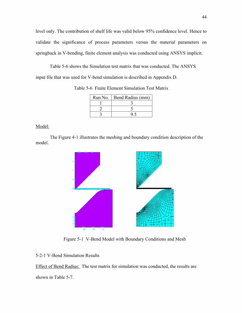
Table 5-6 shows the Simulation test matrix that was conducted. The ANSYS
input file that was used for V-bend simulation is described in Appendix D.
Table 5-6 Finite Element Simulation Test Matrix
Model:
The Figure 4-1 illustrates the meshing and boundary condition description of the model.
Figure 5-1 V-Bend Model with Boundary Conditions and Mesh 5-2-1 V-Bend Simulation Results Effect of Bend Radius: The test matrix for simulation was conducted, the results are shown in Table 5-7.
Run No. Bend Radius (mm)1 3 2 5 3 9.5

45
Table 5-7 V-Bend Simulation Results
Figures below show the simulated results, for 3mm, 5mm and 9.5mm radius. Figure 5-2
shows the exploded view of the sheet under deformation.
Figure 5-2 Simulated Result for Bend Radius 3mm
Figure 5-3 Bend Radius 5mm Figure 5-4 Bend Radius 9.5mm
Run No. Bend Radius (mm)
Springback angle, degrees
1 3 -3.5 2 5 -0.5 3 9.5 4.5

46
Effect of Rolling Direction:
An attempt was made to study the effect of rolling direction on springback using
Barlat’s 2000 anisotropic model. But this attempt was not successful since the user option
in ANSYS implicit does not support contact elements, which are very essential in
simulating sheet metal forming process. Hence this work is recommended for follow-on
studies by using different sheet metal forming codes. In this research, ANSYS implicit,
which is a generic code, was used due to lack of availability of sheet metal forming
codes.

47
CHAPTER VI
DISCUSSION 6-1 Taguchi Experimental results
This study revealed some interesting results. Negative springback or spring-in
was observed in experiments with bend radius less than 5mm. Earlier investigations have
shown that this behavior is noted for thin sheets (R/t < 5, where R is the bend radius and t
is the thickness of the sheet). According to Lembit et al [88], some post-forming
deformations may have occurred during removal of the part from the forming press,
accounting for the flexibility of the thin sheets. Moreover, aluminum alloys are known to
adhere easily to the tools, hence on application of high loads, spring-in may have
occurred on unloading, due to lower flow stresses. Bending at a sharp radius, can cause
the formation of invisible cracks, which might have caused a reduction in springback.
There was no stress cracking observed by light microscopy in the samples tested.
Davies et al [9] found that for ratios of material thickness to bend radius greater
than 0.2, there was a considerable amount of negative springback observed. This is
because the higher the strength, the larger the deformed volume of the material in the
bend. According to Zhang et al [10] as the punch pushes down, the two ends of the
specimens

48
are forced towards the die surfaces and some plastic deformation may occur in the two
contact regions of the specimen with the die resulting in negative springback. Other
effects of various factors on springback are discussed below.
6-1-1 Effect of Bend Radius
Table 5-2 shows that bend radius has a significant effect on springback, and it
overshadows all the other factors. Figure 6-1 shows the sectional profiles of specimens at
various bend radii after forming. Livatyali et al [4] showed that at smaller bending radii,
the sheet is deformed more locally and severely, resulting in the increased plastic
stiffness of the bent zone, and hence creep would be reduced. Investigations show that the
stress over the punch corner is the most significant factor that governs the magnitude of
springback. Hence, springback is greater for the larger die radius this is due to the
comparatively small bending stress locked into the sheet at the punch corner [67].
According to Forcellese [89] when the sheet is bent with a smaller radius, the metal under
the punch is stressed beyond the yield strength through almost the entire sheet thickness.
Such enlargement of the plastic zone produces a reduction in the springback angle.
Figure 6-1 V-Bends at Different Bend Radii
3mm
5mm
9.5mm
3mm
5mm
9.5mm

49
Angle Variation after Bending
-5-4-3-2-1012345
Bend radii, mm
Sprin
g-ba
ck a
ngle
, de
gree
s
Figure 6-2 Variation of Springback Angle with Respect to Different Bend Radii
Gardiner [90] conducted V-bend experiments to measure springback and studied
the effect of bend radius. In this study tests with small bend radii were most difficult to
conduct and resulted in a large data scatter. However, the experimental results shown in
Figure 6-2 illustrate less scatter in the springback angle at small bend radius. Huang et al
[91] conducted experiments for springback of small radius-to-thickness bends in the
range R/t<10, and showed larger springback than that predicted by any known theory.
6-1-2 Effect of Other Factors
Previous investigations have shown that using thicker material will reduce
springback. Forcellese et al [89] showed that for a given radius of the outer fiber under
loading, the increase in the sheet thickness leads to an increase in the bending moment
and the bending strain at the outer fiber, thus reducing the springback angle. In our study,
the contribution of sheet thickness to springback is not significant when compared to
bend radius. Foecke et al [92] has shown that sheets with finer grain sizes, particularly at
3mm 5mm
9.5mm

50
the surface, develop less roughening and have better formability characteristics. That is
springback is reduced when the material has a finer grain size. Present results show that
grain size is significant only to a very small extent.
Sheet metals that exhibit different flow strengths in different directions in the
plane of the sheet are defined as having planar anisotropy [6]. Parallel, perpendicular and
forty-five degrees to the rolling direction represent the three vectors of the planar
anisotropy. Leu [17] showed that anisotropy has a great effect on the bending limit with
the relative differences in yield strength. Springback is reported higher at higher strength,
reflecting minimal spring observed for the bend perpendicular to the rolling direction. In
this study the rolling direction was found to be somewhat significant.
According to Jian Cao et al [15] setting the punch speed to the maximum possible
press value is desired to reach the highest production rate. Shelf life and dwell time are
linearly proportional to the springback behavior; this may be related to the creep
characteristics of aluminum alloy. Present results have shown that shelf life has very little
effect on springback. Contribution of punch speed and dwell time to springback are
almost negligible when compared to bend radius in this study.
6-1-3 Other Defects Observed
Visible surface roughness in regions of the part, which have undergone
appreciable deformation, is called orange peeling. It occurs on free surfaces of metal
alloys where neighboring grains on the surface have different orientation [5]. Orange peel
effects were observed for run numbers 1 and 11, the cause for this is smaller bend radius.
However, the samples heat-treated to increase grain size, did not show orange peel. Using

51
finer-grain-size sheet metal, where the grains deform more nearly as a whole, can reduce
this condition.
6-2 Finite Element Simulation Results
A 2-D finite element model with multilinear isotropic material description gives a
good prediction of springback. Although an attempt that was made to study the effect of
texture (planar anisotropy) on springback was not successful. This might well be a topic
for further study. The Barlat’s 2000 anisotropic model is not defined in ANSYS implicit
code and can be user defined. But the user option in ANSYS implicit code does not
support contact elements, which are essential in simulating sheet metal forming process.
Hence this specific aspect is recommended for follow-on studies by using different sheet
metal forming codes, which support material models that describe the anomalous
behavior of highly textured aluminum alloys.
6-3 Comparison of Experimental and Simulation Results
-5-4-3-2-1012345
Bend radius
Spr
ingb
ack
angl
e, d
egre
es
Experimental
Finite ElementAnalysis
Figure 6-3 Comparison of Experimental and Simulation Results
3mm
5mm
9.5mm

52
There appears to be only a small difference in the experimental and simulation
results, the difference being less than one degree, this shows that the isotropic material
model works well in the prediction of springback. Two important points should be noted
in this context:
1. Figure 3-1 shows that the batch of 6022-T4 AA material used for this study
possesses equiaxed grains; this may well contribute to the material being
isotropic.
2. The grain size of the material as seen in Figure 3-1 was observed to be 40µm,
which is very small. It is presumed that the material was recrystallized and
processed to render it nearly isotropic so that the anomalous behavior is taken
care of.
6-4 Orientation Imaging Microscopy
To crosscheck our results for the texture of the sheet metal, an image analysis of
the as-received 6022-T4 AA material was performed by INCA Inc. Figure 6-4 shows the
OIM images of the 6022 material and it can be observed that the grain size is random.
There is no indication of texture in this rolled material. The color of the grains is not
uniform; it is spread out indicating that the material is nearly isotropic.

53
Figure 6-4 OIM Images for 6022-T4 AA Material as per INCA Inc.

54
CHAPTER VII
CONCLUSIONS
Experimental measurement and finite element simulation of springback on V-
bending 6022-T4 AA was conducted. The relative contribution of process and material
parameters on springback was evaluated using a Taguchi Design of experiment approach.
Experimental predictions showed that the bend radius has the greatest effect on
springback, and it overshadows the other parameters. Spring-in or negative springback
was observed for very small bend radii. Grain size/microstructure showed very little
effect on springback at 95% confidence level. Texture, which showed 15.33%
contribution to springback in the S/N (signal to noise) ANOVA, was significant at only
about 95% confidence level. The other factors studied have negligible effect on
springback when compared to bend radius.
Finite element simulation of springback using ANSYS implicit was conducted to
explore the limits regarding process control by boundary values versus material
parameters. A 2-D model with multilinear isotropic material description was considered.
The experimental results compare well with the simulated results for the effect of bend
radius on springback. Thus proving that the microstructure of the material used in this
study was processed to render it nearly isotropic.

55
CHAPTER VIII
RECOMMENDED FOLLOW-ON STUDIES
In summary, this work evaluated the relative contribution of various process
parameters in addition to material parameters on springback. This springback study went
beyond the work of others as previous investigations have studied only the effect of
certain process or material parameters on springback. Also, this research throws light on
whether the process is driven by boundary values rather than material issues.
Experimental results have shown that though texture had some effect on
springback, it was significant at only 95% confidence level. Finite element results with
isotropic model were in good agreement with the experimental predictions, thereby
proving that the material received from Alcoa was processed to make it nearly isotropic.
An attempt was made to verify the experimental results as to the effect of texture
on springback with finite element analysis using ANSYS implicit code. But this was not
possible due to the limitation of the code, as its user option does not support contact
elements that are required in sheet metal forming simulation. This is an important issue
that needs to be researched by using sheet metal forming codes.
Another important area that needs to be researched is the study of the critical
degree of texture in sheet metal that would require anisotropy. The effect of anisotropy
on springback can be investigated by increasing the texture of the material.

56
REFERENCE
1. T.C. Hsu and I. R. Shien, “Finite Element Modeling of Sheet Forming Process
with Bending Effects,” Journal of Materials Processing Technology, 63, 1997, pp. 733-737.
2. W. Johnson and A.N. Singh, Large Deformations, ed. N. K. Gupta and S.
Sengupta (Delhi: South Asian Publishers Pvt. Ltd., 1982), pp. 236-250.
3. Z.T. Zhang and D. Lee, “Effect of Process Variables and Material Properties on the Springback Behavior of 2D-Draw Bending Parts,” Automotive stamping technology, 1995, pp. 11-18.
4. H. Livatyali and T. Altan, “Prediction and Elimination of Springback in Straight
Flanging Using Computer Aided Design Methods, Part 1: Experimental Investigation,” Journal of Materials Processing Technology, 117, 2001, pp. 262-268.
5. W.F. Hosford and R.M. Caddell, Metal Forming: Mechanics and Metallurgy, 2nd
ed. (New York, NY: Prentice-Hall, 1993).
6. R.G. Davies, C.C. Chu, and Y.C. Liu, “Recent Progress on the Understanding of Springback,” Computer Modeling of Sheet Metal Forming Process: Theory,” 1985, pp. 259-271.
7. Z. Tan, B. Persson and C. Magnusson, “An Empiric Model for Controlling
Springback in V-die Bending of Sheet Metals,” Journal of Materials Processing Technology, 34, 1992, pp. 449-455.
8. R.L. Rolf and E.P. Patrick, “Bending and Springback of Aluminum Alloy Sheet
and Plate,” Formability Topics-Metallic Materials, ASTM STP 647, 1978, pp. 65-85.
9. R.G. Davies and Y.C. Liu, “Control of Springback in a Flanging Operation,”
Journal of Applied Metalworking, 3, no. 2, 1984, pp. 142-147.
10. L.C. Zhang, G. Lu and S.C Leong, “V-Shaped Sheet Forming by Deformable Punches,” Journal of Materials Processing Technology, 63, 1997, pp. 134-139.
57
11. B.S Levy, “Empirically Derived Equations for Predicting Springback in Bending,” Journal of Applied Metalworking, 3, no. 2, 1984, pp. 135-141.
12. C. Wang, G. Kinzel and T. Altan, “Mathematical Modeling of Plane-Strain
Bending of Sheet and Plate,” Journal of Materials Processing Technology, 39, 1993, pp. 279-304.
13. W.Y. Fowlkes and C.M. Creveling, Engineering Methods for Robust Product
Design (Massachusetts, MA: Addison Wesley Longman, Inc., 1995).
14. C. D. Joseph, J. A. Schneider, G. Harlow, “Formability Issues of Auto-Body Materials,” Proceedings of the ASME Southeastern Region XI Technical Conference, 2, no. 1, April 2003.
15. Jian Cao, Brad L Kinsey et al., “Next Generation Stamping Dies-Controllability
and Flexibility”. Robotics and Computer Integrated Manufacturing, 17, 2001, pp. 49-56
16. Chuantao Wang, Gary Kinzel, Taylan Altan, “Mathematical Modeling of Plane-
Strain Bending of Sheet and Plate”. Journal of Materials Processing Technology, 39, 1993, pp. 279-304.
17. D.K. Leu, “A Simplified Approach for Evaluating Bendability and Springback in
Plastic Bending of Anisotropic Sheet Metals,” Journal of Materials Processing Technology, 66, 1997, pp. 9-17.
18. Hisashi Hayashi, “The Control of Shape Fixation and Springback of Aluminum
Alloy Sheet in Model Forming,” The Institute of Physical and Chemical Research (RIKEN), 1996, pp. 115-123.
19. M. Samuel, “Experimental and Numerical Prediction of Springback and Side
Wall Curl in U-Bendings of Anisotropic Sheet Metals,” Journal of Materials Processing Technology, 105, 2000, pp. 382-393.
20. Z.T. Zhang and D. Lee, “Springback Analysis and Control in Forming Two-Step
Rail-Shaped Sheet Metal Parts,” Society of Automotive Engineers, 1996, pp. 51-59.
21. www.scioncorp.com
22. F. Barlat, J. C. Brem, Y.W. Yoon et al., “Plane Stress Yield Function for
Aluminum Alloy Sheets”. International Journal of Plasticity, Dec. 2001.
23. W.D Carden et al, “Measurement of Springback,” International Journal of Mechanical Sciences, 44, 2002, pp.79-101.

58
24. R.G. Davies, Journal of Applied Metalworking, 1 no. 4, 1981, pp. 45-52.
25. C.C. Chu, “Elastic-Plastic Springback of Sheet Metals Subjected to Complex Plane Strain Bending Histories,” International Journal of Solids and Structures, 22, no. 10, 1986, pp.1071-1081.
26. N.M. Wang, “Predicting the Effect of Die Gap on Flange Springback”. 13th
Biennial Congress International Deep Drawing Research Group, Feb. 20-25, 1984, pp.133-147.
27. K. P. Li, W.P. Carden and R. H. Wagoner, “Simulation of Springback”.
International Journal of Mechanical Sciences, 44, 2002, pp.103-122.
28. W. Kubli, J. Reissner, “Optimization of Sheet-Metal Forming Process Using the Special-Purpose Program AUTOFORM”. Journal of Materials Processing Technology, 50, 1995, pp. 292-305.
29. J.N. Reddy, An Introduction to Finite Element Method, Mc Graw Hill, Inc., 2nd
ed., 1993.
30. Kiyoshi Kamita, Takamichi Arakawa, Hiroshi Fukiharu and Akitake Makinouchi, “Evaluation of Geometrical Defects by Finite Element Simulation in the Sheet Metal Forming Processes,” European Congress on Computational Methods in Applied Sciences and Engineering, ECCOMAS, 2000.
31. Hideyuki Sunaga and Akitake Makinouchi, “Sheet Metal Forming Simulation
System for Predicting Failures in Stamping Products,” RIKEN review No.14 December 1996, pp. 47-48.
32. Paulsen F, Welo T., “Applications of Numerical Simulation in the Bending of
Aluminum-Alloy Profiles,” Journal of Materials Processing Technology, 58, 1996, pp. 274-85.
33. Clausen A H, Hopperstad O S, Langseth M., “Stretch Bending Analyses Using
Implicit and Explicit FE Codes,” Proceedings of the 10th Nordic Seminar on Computational Mechanics, Tallinn, Estonia, 1997.
34. Narkeeran Narasimhan, Michael Lovell, “Predicting Springback in Sheet Metal
Forming: An Explicit to Implicit Sequential Solution Procedure,” Finite Elements in Analysis and Design, 33, 1999, pp. 29-42.
35. M J Finn, P C Galbraith, L Wu, J O Hallquist, L Lum, T L Lin, “Use of a Coupled
Explicit-Implict Solver for Calculating Spring-Back in Automotive Body Panels,” Journal of Materials Processing Technology, 50, 1995, pp. 395-409.
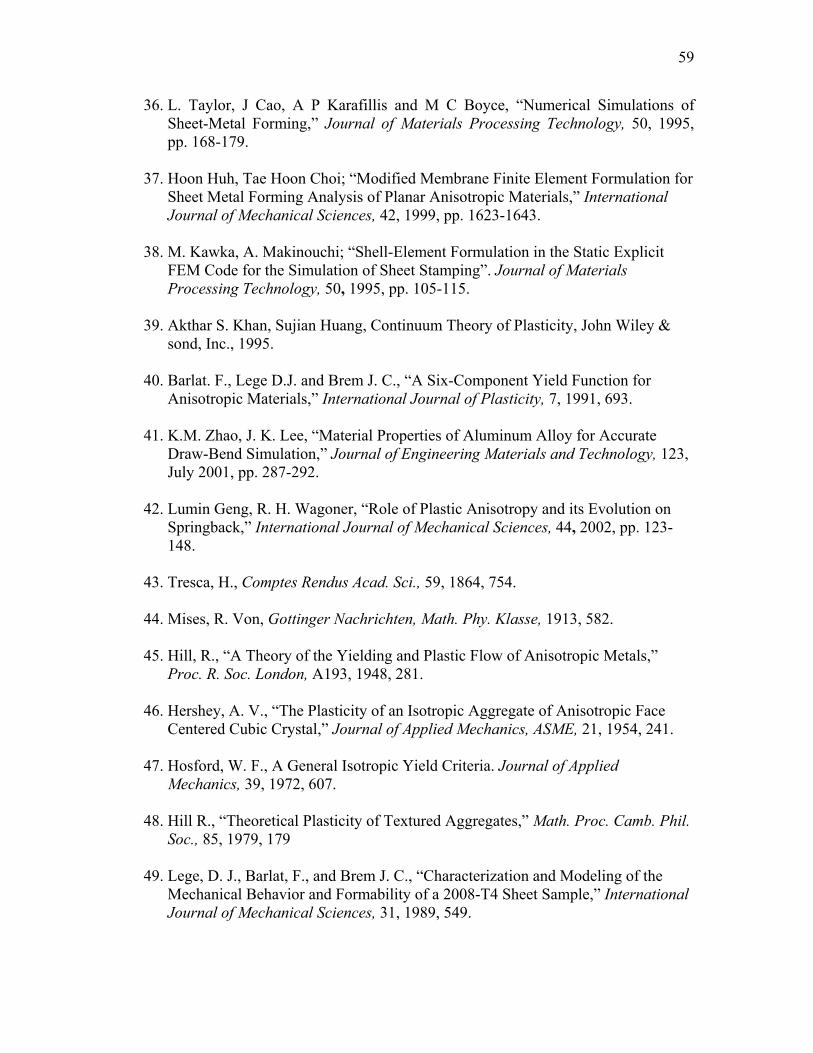
59
36. L. Taylor, J Cao, A P Karafillis and M C Boyce, “Numerical Simulations of Sheet-Metal Forming,” Journal of Materials Processing Technology, 50, 1995, pp. 168-179.
37. Hoon Huh, Tae Hoon Choi; “Modified Membrane Finite Element Formulation for
Sheet Metal Forming Analysis of Planar Anisotropic Materials,” International Journal of Mechanical Sciences, 42, 1999, pp. 1623-1643.
38. M. Kawka, A. Makinouchi; “Shell-Element Formulation in the Static Explicit
FEM Code for the Simulation of Sheet Stamping”. Journal of Materials Processing Technology, 50, 1995, pp. 105-115.
39. Akthar S. Khan, Sujian Huang, Continuum Theory of Plasticity, John Wiley &
sond, Inc., 1995.
40. Barlat. F., Lege D.J. and Brem J. C., “A Six-Component Yield Function for Anisotropic Materials,” International Journal of Plasticity, 7, 1991, 693.
41. K.M. Zhao, J. K. Lee, “Material Properties of Aluminum Alloy for Accurate
Draw-Bend Simulation,” Journal of Engineering Materials and Technology, 123, July 2001, pp. 287-292.
42. Lumin Geng, R. H. Wagoner, “Role of Plastic Anisotropy and its Evolution on
Springback,” International Journal of Mechanical Sciences, 44, 2002, pp. 123-148.
43. Tresca, H., Comptes Rendus Acad. Sci., 59, 1864, 754.
44. Mises, R. Von, Gottinger Nachrichten, Math. Phy. Klasse, 1913, 582.
45. Hill, R., “A Theory of the Yielding and Plastic Flow of Anisotropic Metals,”
Proc. R. Soc. London, A193, 1948, 281.
46. Hershey, A. V., “The Plasticity of an Isotropic Aggregate of Anisotropic Face Centered Cubic Crystal,” Journal of Applied Mechanics, ASME, 21, 1954, 241.
47. Hosford, W. F., A General Isotropic Yield Criteria. Journal of Applied
Mechanics, 39, 1972, 607.
48. Hill R., “Theoretical Plasticity of Textured Aggregates,” Math. Proc. Camb. Phil. Soc., 85, 1979, 179
49. Lege, D. J., Barlat, F., and Brem J. C., “Characterization and Modeling of the
Mechanical Behavior and Formability of a 2008-T4 Sheet Sample,” International Journal of Mechanical Sciences, 31, 1989, 549.

60
50. Barlat, F., Lian J, “Plastic Behavior and Stretchability of Sheet Metals, Part I: A Yield Function for Orthotropic Sheet Under Plane Stress Conditions,” International Journal of plasticity, 5, 1989, 51.
51. A.P. Karafillis and M.C. Boyce, “A General Anisotropic Yield Criterion Using
Bounds and a Transformation Weighting Tensor,” Journal of Mech. Phy. Solids, 41, no.12, 1993, pp. 1859-1886.
52. P. Ducroco, E. Markiewicz, P. Drazetic, and P Guyon, “An Inverse Approach to
Determine the Constitutive Model Parameters Using Drop Tests and Numerical Tools,” International Journal of Impact Engineering, v 21, n 6, Jul, 1998, p 433-449.
53. J. Y. Sheikh-Ahmad, J.A. Bailey, “A Constitutive Model for Commercially Pure
Titanium,” Journal of Engineering Materials and Technology, 117, April 1995, pp. 139-144.
54. J.P Noble and J. Harding, “An Evaluation of Constitutive Relations for High-Rate
Material Behavior Using the Tensile Hopkinson Bar,” Journal De Physique IV, 4, September 1994, pp. C8-477 to C8-482.
55. R.D. Krieg, S.W Key, “Implementation of a Time Dependent Plasticity Theory
into Structural Computer Programs,” American Society of Mechanical Engineers, Applied Mechanics Division, AMD, v 20, 1976, p 125-137
56. S.G. Cochran, M.W. Guinan, D.J. Steinberg, “Constitutive Model for Metals
Applicable at High-Strain Rate,” Journal of Applied Physics, v 51, n 3, Mar, 1980, p 1498-1504
57. G.R. Johnson, W.H. Cook, “A Constitutive Model and Data for Metals Subjected
to Large Strains, High Strain Rates and High Temperatures,” Proceedings of the 7th International Symposium on Ballistics, 1983, pp. 541-547.
58. N. Jones, J.G. Oliveira, “Impulsive Loading of a Cylindrical Shell with
Transverse Shear and Rotatory Inertia,”International Journal of Solids and Structures, v 19, n 3, 1983, p 263-279
59. F.J. Zerilli and R.W. Armstrong, “Constitutive Equation for HCP Metals and
High Strength Alloy Steels,” American Society of Mechanical Engineers, Aerospace Division (Publication) AD, v 48, High Strain Rate Effects on Polymer, Metal and Ceramic Matrix Composites and Other Advanced Materials, 1995, p 121-126
60. W.J. Wang, S.S. Cho, H. Huh and D.T. Chung, “Modified Johnson-Cook Model
for Vehicle Body Crashworthiness Simulation,” International Journal of Vehicle Design, 21, nos. 4/5, 1999, pp. 424-435.

61
61. M Y Demeri and S. C Tang, “Post Processing Analysis in Sheet Metal Forming
Simulation,” JOM, June 1992, pp. 14-16.
62. Keecheol Park, Youngsuk Kim, “The Effect of Material and Process Variables on the Stamping Formability of Sheet Materials,” Journal of Materials Processing Technology, 51, 1995, pp. 64-78.
63. K.P. Rao, S.M Doraivelu, “Flow Curves and Deformation of Materials at
Different Temperatures and Strain Rates,” Journal of Mechanical Working Technology, 6, 1982, pp. 63-88.
64. Dong Hongzhi, Lin Zhongqin, “Investigation of Sheet Metal Forming by Numerical Simulation and Experiment,” Journal of Materials Processing Technology, 103, 2002, pp. 404-410.
65. M. Kawka, A. Makinouchi; “Plastic Anisotropy in FEM Analysis Using
Degenerated Solid Element,” Journal of Materials Processing Technology, 60, 1996, pp. 239-242.
66. E. Nakamachi, K. Hiraiwa, H. Morimoto, M. Harimoto; “Elastic/Crystalline
Viscoplastic Finite Element Analyses of Single and Poly-Crystal Sheet Deformations and their Experimental Verification,” International Journal of Plasticity, 16, 2000, pp. 1419-1441.
67. D. Lefebvre, E. Haug, F. Hatt; “Industrial Applications of Computer Simulation
in Stamping,” Journal of Materials Processing Technology, 46, 1994, pp. 351-389.
68. Sven K. Esche, Gary L Kinzel, and Taylan Altan, “Issues in Convergence
Improvement for Non-Linear Finite Element Programs,” International Journal for Numerical Methods in Engineering, 40, 1997, pp. 4577-4594.
69. K C Ho, J Lin, and T A Dean, “Integrated Numerical Procedures for Simulating
Springback in Creep Forming Using ABAQUS,” ABAQUS UK Users Group Conference, 2001.
70. K. Chung and R. H. Wagoner, “Numerical Improvement of Viscoplastic, Non-
Linear Finite Element Analysis,” International Journal of Mechanical Sciences, 29, 1987, pp. 45-59.
71. P. T. Vreede, M. F. M. Louwes, J. Huetink, N A J Langerak, “Contact Behavior
Modeled with Interface Elements and Tool Description,” Proceedings of the 4th International Conference, NUMIFORM 92, 1992, pp. 565-570.

62
72. L. B. Chappius, S.C. Tang, X. M. Chen and J.H. Wu, “A Numerically Stable Computer Model for Sheet Metal Forming Analysis by 2D Membrane Theory,” SAE 930518, 1993.
73. J.K Lee, U.Y. Cho, J. Hambrecht and S Choudhry, “Recent Advances in Sheet
Metal Forming Analysis,” Proceedings of the Winter Annual Meeting, ASME vol. AMD 125, 1991, pp. 119-130.
74. M S Joun and M C Lee, “Quadrilateral Finite-Element Generation and Mesh
Quality Control for Metal Forming Simulation,” International Journal for Numerical Methods in Engineering, 40, 1997, pp. 4059-4075.
75. Morestin, F. Boivin, M. and Silva, C., “Elasto Plastic Formulation Using a
Kinematic Hardening Model for Springback Analysis in Sheet Metal Forming,” Journal of Materials Processing Technology, 56, 1996, pp. 619-630.
76. Zhang, L C and Lin, Z., “An Analytical Solution to Springback of Sheet Metals
Stamped by Rigid Punch and an Elastic Die,” Journal of Materials Processing Technology, 63, 1997, pp. 49-54.
77. Bradley N. Maker, “Implicit Springback Calculation Using LS-DYNA,” 5th
International LS-DYNA Users Conference, 21-22, Sept. Southfield, MI, USA, 1998.
78. Lembit M. Kutt, Jerrell A. Nardiello, Patricia L. Ogilvie et al, “Non-Linear Finite
Element Analysis of Springback,” Communications in Numerical Methods in Engineering, 15, 1999, pp. 33-42.
79. F. Micari, A. Forcellese, L. Fratini, F. Gabrielli and N. Alberti, “Springback
Evaluation in Fully 3-D Sheet Metal Forming Processes”.
80. Annika Nilsson, Lars Melin, Claes Magnusson, “Finite-Element Simulation of V-Die Bending: a Comparison with Experimental Results,” Journal of Materials Processing Technology, 65, 1997, pp. 52-58.
81. You-Min Huang and Daw-Kwei Leu, “Effects of Process Variables on V-Die
Bending Process of Steel Sheet,” International Journal of Mechanical Sciences, 40, no. 7, 1998, pp. 631-650.
82. Huang, Y. M., Lu, Y. H and Makinouchi, A., “Elasto-Plastic Finite-Element
Analysis of V-Shape Sheet Bending,” Journal of Materials Processing Technology, 35, 1992, pp. 129-150.
83. Ogawa, H., Makinouchi, A., Takizawa, H., and Mori, N., “Development of an
Elasto-Plastic FE Code for Accurate Prediction of Springback in Sheet Bending Processes and its Validation by Experiments,” Advanced Technology of Plasticity

63
1993 Proceedings of Fourth International Conference on Technology of Plasticity, pp. 1641-1646.
84. Lee, S W and Yang, D Y., “An Assessment of Numerical Parameters Influencing
Springback in Explicit Finite Element Analysis of Sheet Metal Forming Process,” Journal of Materials Processing Technology, 80-81, 1998, pp. 60-67.
85. Nan Song, Dong Qian, Jian Cao, et al., “Effective Models for Prediction of
Springback in Flanging,” Transactions of the ASME, 123, October 2001, pp. 456-461.
86. Xuechun Li, Yuying Yang, Yongzhi Wang Jun Bao and Shunping Li, “Effect of
the Material-Hardening Mode on the Springback Simulation Accuracy of V-Free Bending,” Journal of Materials Processing Technology, 123, 2002, pp. 209-211.
87. Y.T. Keum, K.B Lee, “Sectional Finite Element Analysis of Forming Processes
for Aluminum Alloy Sheet Metals,” International Journal of Mechanical Sciences, 42, 2000, pp. 1911-1933.
88. Lembit M. Kutt et al, “Non-Linear Finite Element Analysis of Springback.
Communications in Numerical Methods in Engineering,” 15, 1999, pp. 33-42.
89. Forcellese and F. Gabrielli, “Artificial Neural-Network-Based Control System for Springback Compensation in Press-Brake Forming,” International Journal of Materials and Product Technology, 16, nos. 6/7, 2001.
90. F. J Gardiner, “ The Springback of Metals,” Transactions of the ASME, May
1994.
91. Huang, Mai and J.C. Gerdeen, “Springback of Doubly Curved Developable Surfaces - An Overview,” SAE paper 940938, Analysis of autobody stamping technology, SP-1021, SAE international congress, Detroit, MI, 1994, pp.125-138.
92. T. Foecke, S.W. Banovic, and R.J Fields, “Sheet Metal Formability Studies at the
National Institute of Standards and Technology,” JOM, 2001, pp. 27-30.

64
APPENDIX A
UNIAXIAL TENSION TEST RESULTS

65
The Figures A-1 to A-3 illustrates the engineering stress strain plots recorded at
different speeds of the load frame (5.1mm/min and 510mm/min) with three repetitions
each. The uniaxial tests are conducted at 0, 45 and 90 degrees to the rolling direction. As
seen from the plots, there is not much variation in the properties of the material at the
varying speeds; this signifies that the material properties are rate independent.
0 degrees to rolling direction
0
50
100
150
200
250
300
0 0.05 0.1 0.15 0.2 0.25Engineering Strain (mm/mm)
Engi
neer
ing
Stre
ss (M
Pa)
5.1mm/min, run15.1mm/min, run25.1mm/min, run3510mm/min, run1510mm/min, run2510mm/min, run3
Figure A-1 Stress Strain Plot at Different Speeds When Tested 0 Degrees to Rolling Direction
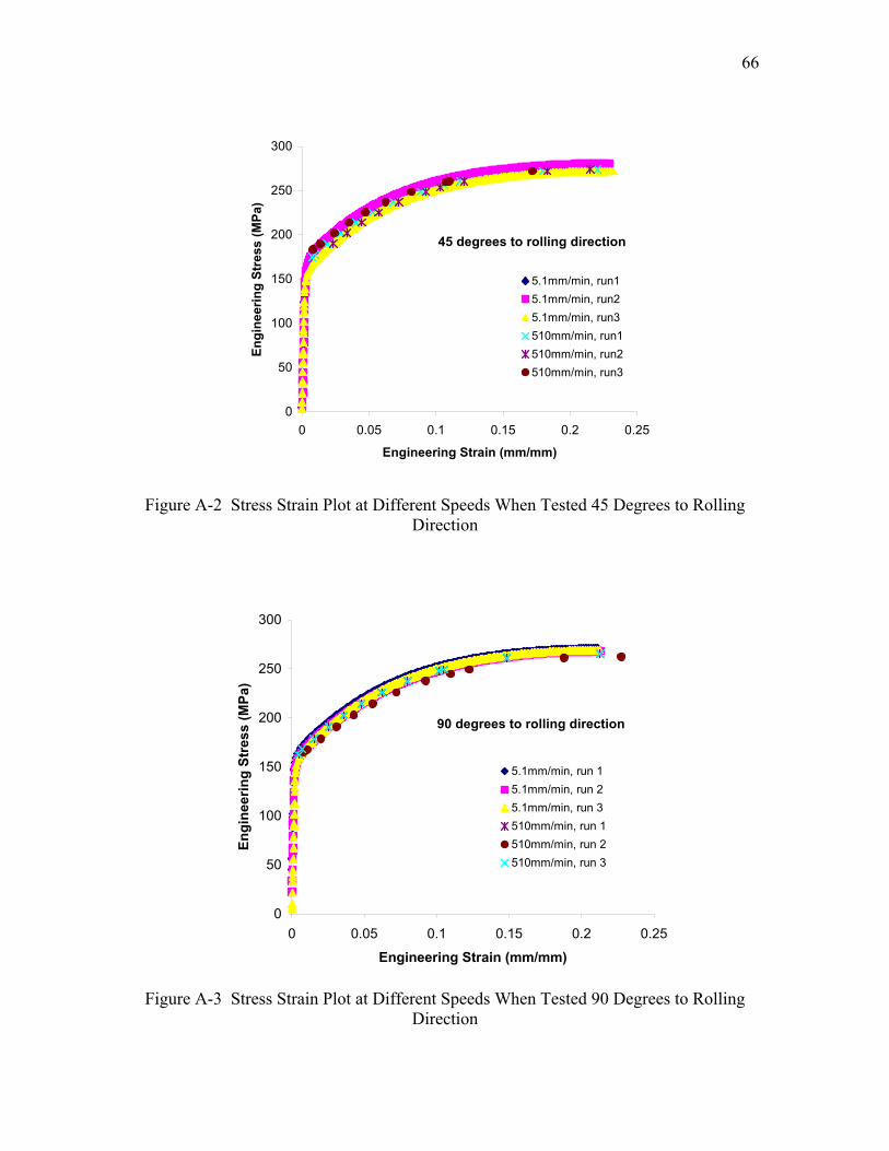
66
45 degrees to rolling direction
0
50
100
150
200
250
300
0 0.05 0.1 0.15 0.2 0.25
Engineering Strain (mm/mm)
Engi
neer
ing
Stre
ss (M
Pa)
5.1mm/min, run15.1mm/min, run25.1mm/min, run3510mm/min, run1510mm/min, run2510mm/min, run3
Figure A-2 Stress Strain Plot at Different Speeds When Tested 45 Degrees to Rolling Direction
90 degrees to rolling direction
0
50
100
150
200
250
300
0 0.05 0.1 0.15 0.2 0.25
Engineering Strain (mm/mm)
Engi
neer
ing
Stre
ss (M
Pa)
5.1mm/min, run 15.1mm/min, run 25.1mm/min, run 3510mm/min, run 1510mm/min, run 2510mm/min, run 3
Figure A-3 Stress Strain Plot at Different Speeds When Tested 90 Degrees to Rolling
Direction

67
Figure A-4 describes the mechanical properties of 6022-T4 AA tested uniaxially
at three directions to the rolling plane, i.e., 0, 45 and 90 degrees. It shows that 0 degrees
has the highest strength followed by 90 degrees. 45 degrees to the rolling plane has the
least strength.
158160162164166168170172
0 45 90 135
Tensile axis angle from rolling (degrees)
Yiel
d St
reng
th (M
PA)
Yield Strength
270
275
280
285
290
0 45 90 135Tensile axis angle from
rolling (degrees)U
TS (M
Pa)
UTS
0
0.10.2
0.3
0.40.5
0.6
0 45 90 135Tensile axis angle to rolling
direction (degrees)
Res
ilien
ce (M
Pa)
Resilience (Work)
45.4
45.6
45.8
46
46.2
46.4
0 45 90 135Tensile axis angle from
rolling (degrees)
Toug
hnes
s (M
Pa)
Toughness

68
00.10.20.30.40.50.60.70.8
0 45 90 135Tension axis angle
from rolling (degrees)
r val
ue
r value [45]
20
20.5
21
21.5
22
22.5
23
0 45 90 135Tensile axis angle to rolling
direction (degrees)
% E
long
atio
n to
Fai
lure
% Elongation toFailure
Figure A-4 Mechanical Properties of 6022-T4 AA

69
APPENDIX B
V-BEND TEST PROCEDURE

70

71
V-Bend Test Procedure
1. Start FT Console; get to live displays (right click on main menu bar). 2. Calibrate/Balance load cell. 3. Start Merlin 4. Set "1 travel - use feeler gauge, lower punch to 30 lb with
"035.0 (sheet thickness) 5. Reset gage length on either load frame or screen right hand side icon, with strain
gage (equal to thickness of sheet metal) 6. At the load frame, jog up or down (fine position controls speed). Set anvil height. 7. Set load and extension limits.
Load limits: Upper transducer limit: Value: 1000 lb Action: Stop Lower transducer limit: Value: -1000 lb Action: Stop Extension limits: Upper transducer limit: Value: "1 Action: Stop Lower transducer limit: Value: - "1 Action: Stop
Note: -1000 lb load stops test 8. Before starting test: ensure that there are no blinking lights. If so, enable loads and
limits, and arm all physical limits. First click on the STOP icon to stop it from blinking.
9. File setup: Save as ASCII raw.dat 10. Start test; After completion of test - store data
File Data
End & save data 11. At completion of test:
Exit Merlin File Exit Exit FT Console Right click on top bar Exit
12. Note: For hold testing, record load before and after hold period Make angle measurements immediately after test.

72
APPENDIX C
TAGUCHI ANALYSIS DESCRIPTION

73
This section describes the statistical evaluation of springback recorded in Table 5-
1 from experimental testing. Analysis of variance is a computational technique that
quantitatively estimates the relative contribution of each control factor to the overall
measured response and expresses it as a percentage.
It uses a mathematical technique known as the sum of squares to quantitatively
examine the deviation of the control factor effect response averages from the overall
experimental mean response. The significance of the individual control factors is
quantified by comparing the variance between the control factor effects against the
variance in the experimental data due to random experimental error and the effects of
unrepresented interactions, this is given by the F-ratio. It is used to test for the
significance of factor effects.
error alexperiment todue squaremean factor control a todue squaremean
=− ratioF
The Taguchi approach, ANOVA can be applied to two forms of data. First, it can be
applied to the data as measured in engineering units to find the relative contribution of
each control factor to the overall measured response. Second, it can be applied to the data
after it has been transformed into S/N ratios. This is done to find the effect of noise due to
repetition of runs.
1. ANOVA (Analysis of Variance)
The first step in this analysis is to calculate the totals for each of the factors and
the error column. The first level of factor A would be represented by all the data points
where the first level of Factor A occurred in the experiment. The first level of factor A

74
occurred in experiments 1, 2, 3, 10, 11, and 12. This is done in the same manner for each
level of each of the factors and the error column. Table C-1 represents the totals table for
the analysis of variance.
Table C-1 Totals Table for Analysis of Variance
Totals Mean A1 -68.5 -3.80556A2 -22.751 -1.26394A3 39.66 2.203333B1 -25.167 -1.39817B2 -15.338 -0.85211B3 -11.086 -0.61589C1 -3.09 -0.17167C2 -24.917 -1.38428C3 -23.584 -1.31022D1 -25.333 -1.40739D2 -16 -0.88889D3 -10.258 -0.56989E1 -17.92 -0.99556E2 -14.838 -0.82433E3 -18.833 -1.04628F1 -18.588 -1.03267F2 -14.587 -0.81039F3 -18.416 -1.02311G1 -24.916 -1.38422G2 -13.338 -0.741 G3 -13.337 -0.74094e1 -17.752 -0.65748e2 -33.839 -1.2533
Sum of Squares: Sum of Squares for the total, ST: Sum of squares for the total is calculated by taking each of the 54 data points,
square them, and from the sum of those squared observations, subtract away the total of
all the data points, squared, divided by the total number of data points, i.e., 54.
ST = (-4.583) 2 + (-4.75) 2+(-3.75) 2 +(-3.333) 2 +……………..+(1.25) 2 - (-51.591) 2

75
54 = 378.047 Sum of Squares for factors:
nnnnS
2
3*
2
2*
2
1*
2
*)3*2*1(*)3(*)2(*)1(* ++
−++=
54)(
181818
2321
23
22
21 AAAAAAS A
++−++=
= 376.82 - 49.29 = 327.53 Similarly for other factors: SB = 55.085 - 49.29 = 5.795 SC = 65.923 - 49.29 = 16.633 SD = 55.72 - 49.29 = 6.43 SE = 49.776 - 49.29 = 0.486 SF = 49.8579 - 49.29 = 0.5679 SG = 54.2547 - 49.29 = 4.9647 Se1 = (-17.752 + 33.839) 2 / 54 = 4.79 Se2 = ST - (SA +…+Se1) = 10.8504 Degrees of Freedom:
The Degrees of Freedom must be calculated for each of the factors, the error term and the
total. The Degrees of Freedom for the total is obtained by taking the total number of data
points and subtracting 1. The Degrees of Freedom for any factor is computed by taking
the number of levels for that factor and subtracting 1. The Degrees of Freedom for Error
is the left over Degrees of Freedom not accounted for by the factors.

76
Total: dfT = n-1 = 54-1 = 53
Factors: dfA…….dfG = 3-1 = 2
Error (primary) dfe1 = 2-1 =1
Error (secondary) dfe2 = dfT - (dfA +dfB +dfC +dfD +dfE +dfF +dfG +dfe1)
= 53-15 = 38
Variance:
Variance is the sum of squares divided by the Degrees of Freedom.
F-Statistic:
A test statistic is now calculated to help test for the significance of the difference that is
demonstrated by the experiment for the outcome of interest. To calculate the F-Statistic
for a factor divide the Variance for that factor by the Variance for error, forming a ratio
of variances. The bigger this ratio is the more difference there is between the levels for a
factor. Thus an initial ANOVA Table is evaluated and is illustrated in Table 5-2.
Since 21 ee VV ≥ the secondary error is discarded and all the factors are tested
versus the primary error
Pooling rules:
1. Factors that have an F-Statistic less than or equal to 1 should be pooled into an
error term and thought of as a random variation component.
2. When after pooling all the factors where the F ratio is less than or equal to 1, the
number of factors remaining is not equal to or less than ½ the number of columns
in the array, then additional pooling must be done.
Calculations for pooled error term: Pooling factors whose F<1 with the error term

77
Se(pool) = SB +SD +SE + SF + SG + Se = 23.034 dfe (pool) = 2*5 + 1 =11 Ve(pool) = Se (pool) / dfe (pool) = 23.034/11 = 2.094 Next, the pure sum of squares must be calculated. This is given by the formula as below:
eAAA VdfSS )(' −= = 323.342
eCCC VdfSS )(' −= = 12.445
eeTee VdfdfSS )(' −+= = 23.034 + (15-11) 2.094 = 31.41 A Percentage Contribution (P%) is also computed for the remaining terms. This is done
by taking the Pure Sum of Squares for each of the terms and dividing by the sum of
squares for total. The pooled ANOVA Table is described in Table 5-3.
Analyzing this pooled ANOVA table. The percentage contribution of error is a
key measure of the successfulness of an experiment. This percentage contribution
explains the leftover variation that was not accounted for by the factors and levels
analyzed in the experiment. A general rule of the thumb is if this percentage contribution
is less than 50% this is a good experiment.
2. S/N (Signal to Noise) ANOVA
The next step would be to reduce and analyze the data to find the effect of noise
due to repetitions of runs. The smaller the better type of analysis is used in this regard.

78
The signal-to-noise metric is designed to be used to optimize the robustness of a product
or process. The smaller the better type S/N ratio is given by,
]log[10/ 22 ySNS STB +−=
where, y is the mean, which is defined as the central tendency of the sample data and it is given by,
∑=
=n
iiy
ny
1
1
The variability of sample data is given by the sample variance, 2S ,
∑=
−−
=n
ii yy
nS
1
22 )(1
1
Table C-2 shows the S/N ratios of the 18 runs.
Table C-2 Signal to Noise Ratios for the V-Bend Experiments
Run #
Factors Springback angle (radians): 3 test points
Mean S/N ratio
e A B C D E F G (a) (b) (c) 1 1 1 1 1 1 1 1 1 -4.583 -4.75 -3.75 -4.361 -12.859 2 1 1 2 2 2 2 2 2 -3.333 -3.417 -3.667 -3.472 -10.823 3 1 1 3 3 3 3 3 3 -3.333 -3.0 -3.5 -3.278 -10.338 4 1 2 1 1 2 2 3 3 0 -0.583 0.583 -0.389 5.774 5 1 2 2 2 3 3 1 1 -1.5 -1.25 -0.917 -1.22 -1.970 6 1 2 3 3 1 1 2 2 -0.917 -1.0 -0.583 -0.833 1.293 7 1 3 1 2 1 3 2 3 2.417 0.667 1 1.361 -4.339 8 1 3 2 3 2 1 3 1 2.167 1.5 1.417 1.695 -4.832 9 1 3 3 1 3 2 1 2 4.25 4.5 3.83 4.194 -12.481 10 2 1 1 3 3 2 2 1 -3.75 -4.917 -4.75 -4.472 -13.096 11 2 1 2 1 1 3 3 2 -3.75 -3.5 -3.0 -3.417 -10.727 12 2 1 3 2 2 1 1 3 -4.167 -4 -3.333 -3.833 -11.728 13 2 2 1 2 3 1 3 2 -2.167 -2.833 -1.667 -2.22 -7.219 14 2 2 2 3 1 2 1 3 -1.417 -2.25 -3.167 -2.278 -7.749 15 2 2 3 1 2 3 2 1 -0.833 -0.833 -1.417 -1.028 -0.683 16 2 3 1 3 2 3 1 2 1.333 1.333 1.25 1.305 -2.318 17 2 3 2 1 3 1 2 3 3.583 3.833 3.33 3.582 -11.104 18 2 3 3 2 1 2 3 1 1.5 0.5 1.25 1.083 -1.595

79
The overall mean S/N ratio ( NS / ) for the entire matrix experiment is the
reference point from which the variance of each control factor’s S/N averages is
calculated by summing the squared deviations from the overall mean.
The ANOVA process begins by determining the grand total sum of squares (GTSS):
∑=
=18
1
2)/(i
iNSGTSS
= (-12.859) 2 + (-10.823) 2 +. ………+ (-1.595) 2
= 1294.082
The GTSS can be decomposed into two parts:
1. The sum of the squares due to the overall experimental mean:
SS due to the overall experimental mean = (# of experiments) * 2
/ NS
= 18*(-6.48839) 2
= 757.7856 2. The sum of the squares due to variation about the mean, referred to as the total
sum of the squares:
Total sum of squares = 2
18
1)//( NSNSS
iiT −= ∑
=
=536.30
Note that the grand total SS = total SS + SS due to mean.
The experiment is structured such that the orthogonal (balanced) nature of the design
produces data that must be gathered in the following format, for the L18:
- Six runs for A at level 1 (runs 1, 2, 3, 10, 11, 12)
- Six runs for A at level 2 (runs 4, 5, 6, 13, 14, 15)
- Six runs for A at level 3 (runs 7, 8, 9, 16, 17, 18)

80
Therefore, for factor A, the sum of squares due to variation about the mean is;
22
21 )//)(2.exp(#)//)(1.exp(# NSNSatAofNSNSatAofS AAA −+−=
23 )//)(3.exp(# NSNSatAof A −+
2
32
22
1 )//(6)//(6)//(6 NSNSNSNSNSNS AAA −+−+−=
222 )5.6111.6(6)5.6759.1(6)5.65947.11(6 +−++−++−=
= 291.493
where 1/ ANS is the average of the 6 samples for each level (I = 1, 2, or 3) This procedure is repeated for the remaining factors and their sum of squares are as
follows:
BS = 17.2979
CS = 2.5097
DS = 85.3867
ES = 21.79449
FS = 33.899244
GS = 4.447
1eS = 13.5995
2eS , gives the sum of squares for the secondary error.
12 eGFEDCBATe SSSSSSSSSS −−−−−−−−=
= 65.88
Degrees of Freedom:
Total: dfT = n-1 = 54-1 = 53

81
Factors: dfA…….dfG = 3-1 = 2
Error (primary) dfe1 = 2-1 =1
Error (secondary) dfe2 = dfT - (dfA +dfB +dfC +dfD +dfE +dfF +dfG +dfe1)
= 53-15 = 38
Variance and F-Statistics are calculated as in the previous ANOVA analysis. The initial
S/N ANOVA Table is shown in Table 5-4. Pooling is done in a similar fashion as
described before.
Calculations for pooled error term: Pooling factors whose F<1 with the error term Se(pool) = SB +SC +SE + SG + Se = 59.6486 dfe (pool) = 2*4 + 1 =9 Ve(pool) = Se (pool) / dfe (pool) = 59.6486/9 = 6.627 Next, the pure sum of squares must be calculated. This is given by the formula as below:
eAAA VdfSS )(' −= = 278.2378
eDDD VdfSS )(' −= = 72.1327
eFFF VdfSS )(' −= = 20.645
eeTee VdfdfSS )(' −+= = 59.6486 + (15-9) * (6.627) = 99.4106 The pooled ANOVA table is illustrated in Table 5-5.

82
APPENDIX D
ANSYS INPUT FILE MAC.DAT FOR CHAPTER V,
V-BEND SIMULATION

83
ANSYS Input file mac.dat for Chapter V, V-bend simulation
RESUME FINISH Timevar=0 Nsteps=183 !Number of step Dismax=-0.1 secdis=-0.0574 /solu AUTOTS,ON NSEL,s,LOC,Y,59,60 CM,CMNODES,NODE Cmsel,all nsel,all esel,all *DO,J,1,Nsteps TimeVar=Timevar+1 *if,J,gt,183,then RStrs=Rstrs+secdis *else RStrs=dismax*j *endif Time,TimeVar CMSEL,S,CMNODES D,all,uy,rstrs nsel,all esel,all SOLVE SAVE *enddo ! Unloading Nsteps=28 *DO,J,1,Nsteps TimeVar=Timevar+1 *if,J,eq,1,then RStrs=Rstrs-secdis *else RStrs=Rstrs-dismax *endif Time,TimeVar CMSEL,S,CMNODES D,all,uy,rstrs nsel,all esel,all SOLVE SAVE *enddo