Evidence on the existence of speculative bubbles in farmland prices

Journal of Real Estate Finance and Economics, 6:223-236 (1993) �9 1993 Kluwer Academic Publishers

Evidence on the Existence of Speculative Bubbles in Farmland Prices

ABEBAYEHU TEGENE AND FREDERICK R. KUCHLER Economic Research Service, U.S. Department of Agriculture, 1301 NY Ave. NW,, Washington, DC20005-4788

Abstract

We conduct tests for the contribution of speculative bubbles to farmland prices. These tests are carried out under the hypothesis that farmland investors rationally form expectations. The outcome of tests reported here allows us to infer whether farmland prices are determined by market fundamentals--discounted returns from the highest economic land use--or whether rumors about farmland price movements are self-fulfilling. The tests are stationarity and cointegmtion tests relating farmland prices to rents. The tests are carried out using data from three farm production regions--the Corn Belt, the Northern Plains, and the Lake States. In each region, we find little evidence to reject the hypothesis that market fundamentals determine farmland prices.

Key words: Farmland prices, Rental rates, Speculative bubbles, Market fundamentals, Unit root, Stationarity, Cointegration

1. Introduct ion

This article examines some of the evidence for the existence of speculative bubbles in farmland prices. We examine farmland price behavior across the North Central region, the prin- cipal agricultural region of the United States. There is some circumstantial evidence sup- porting the existence of a speculative bubble. We test for the presence of speculative bubbles in farmland prices, assuming that farmland investors can be characterized as forming rational expectations.

The long run, stable relation between farmland prices and returns leads us to infer that bubbles do not exist. We conclude market fundamentals determine, and have determined, farmland prices. The approach we adopt draws on the methods developed by Campbell and Shiller (1987) and Diba and Grossman (1988). Falk (1988) used these methods to test for the existence of speculative bubbles in Iowa farmland prices. His results suggested the non-existence of bubbles. We examine three multi-state regions, and our results leave less doubt that Falk 's results were unique and specific to one state. We also give special atten- tion to the 1970s, the per iod when speculative bubbles are alleged to have occurred.

During the 1970s, farmland prices increased rapidly. Many farmland market observers commented that farmland prices reflected speculative mania rather than market fundamentals (Featherstone and Baker, 1987; Paarlberg, 1980; Plaxico, 1979). The existence of speculative mania, often called a bubble, means that investors purchase farm real estate on the assumption of future sales at higher prices, and not on the basis of expected income calculations. Some commented that the farm debt crisis logically followed such speculation (Belongia, 1985).

224 ABEBAYEHU TEGENE AND FREDERICK R. KUCHLER

If these market observers are correct and the farmland market is subject to speculative bubbles, then existing federal farm policies would not be useful tools for guiding farm income or the wealth of the agricultural sector. Any support program influencing current income would be almost irrelevant to farmland investors during the upswing in farmland prices and might not offer enough income support to investors who bought farmland at the price peak to support their debt levels when the bubble inevitably bursts.

The presence of a price bubble is revealed by evidence that asset prices rise (or fall) over an extended period without similar changes in returns. When market fundamentals determine asset prices, any of the forces that determine the present value of expected earnings from asset ownership--including anticipated changes in demand for the commodity the asset produces, discount rates, government programs, or production costs--can explain price changes. When speculative bubbles drive asset prices, any connection between price changes and market fundamentals, including government programs, will be relatively small. Price changes resulting from speculative mania could quickly swamp changes attributable to market fundamentals.

This paper focuses on three regions within the North Central United States: (1) the Lake States (Michigan, Wisconsin, Minnesota); (2) the Corn Belt (Ohio, Indiana, Illinois, Iowa, Missouri); and (3) the Northern Plains (North Dakota, South Dakota, Nebraska, Kansas). These regions are major agricultural regions in the U.S., and they have experienced putatively large land price swings in the 1970s and 1980s. Second, these regions' farmland prices are probably less influenced by urban pressure than elsewhere. Farmland values are more closely related to farm activities than elsewhere. Finally, leasing is a common practice in these regions. 1 Hence, observed rent series can be used as a good proxy for returns to land (farming) 2

Some evidence for the existence of a speculative bubble is considered in Section 2. Characteristics of land prices and returns with and without speculative bubbles are presented in Section 3. Section 4 is a description of the data and empirical results. Concluding remarks are made in Section 5.

2. The Evidence

During the 1970s, the rates at which farmland price gains accrued were greatest in the Corn Belt states, although other states in the central U.S. displayed similar patterns. In Iowa, for example, average per-acre values more than quadrupled between 1970 and 1980. In- vestors who bought farmland at the price peak (1981) experienced a 60 percent capital loss over the following six years, measured in nominal terms. In real terms, in the Corn Belt, Lake States, and Northern Plains regions, when values bottomed out they were similar to values reached in the mid-1960s. All the gains of the 1970s were gone (U.S. Department of Agriculture, Economic Research Service, 1989 and earlier issues).

A market displaying a bubble in asset prices differs from markets in which bubbles are absent because a bubble will cause prices and returns to diverge. In an efficient asset market, today's price will be equivalent to the sum of tomorrow's anticipated price and anticipated earnings, discounted back to today. The presence of a bubble implies there is an additional element determining price--the bubble--which can grow at the discount rate without violating market efficiency and rational asset price expectations (Diba, 1990).

EVIDENCE ON THE EXISTENCE OF SPECULATIVE BUBBLES IN FARMLAND PRICES 225

An assumption common to the land value literature is that the value of land is equal to the present value of projected returns from the land. One measure of the return from land is the rent that a tenant is willing to pay to acquire control of the land. Let Pt denote the real price per acre of farmland, traded at the beginning of period t. Let R t denote the real rent in period t that can be obtained from the ownership of an acre of land. Farmland price can be expressed as:

o o

P, = a~__a aiE(g,+ilI,) i=0

(1)

where a = (1 + r) -1 is the discount rateS; r is the constant real interest rate; E denotes conditional mathematical expectations, assumed to be equivalent to linear projections; and It is the information set at time t. It is assumed to contain, at a minimum Pt, Pt-a, �9 . .

and Rt, Rt-1, . . . Equation (1) is derived from a standard efficient market model (see, for example, West,

1987):

Pt = aE[ (P t+ l + Rt)]/t)] (2)

Equation (1) is one of many possible solutions to equation (2). Applying the law of iterated expectations and solving equation (2) recursively, we obtain:

T

Pt = aZa iE(R t+i l l t ) + arE(Pt+rllt) (3)

i=0

If the transversality condition

limr-~oo arE(Pt+ Tllt) = 0

holds, then Pt = Pt*, where o o

* I,,,) Pt = a aiE(Rt+i i=0

(4)

(5)

Ptdefined in (5) is the unique forward solution to equation (2) as long as the transversality condition (4) holds (West, 1987). Thus, the present value model given by equation (1) is a solution to the arbitrage relation (2) only if condition (4) holds.

If the transversality condition fails, there is a family of solutions to equation (2) (Taylor, 1977); Blanchard and Watson, 1982; West, 1987). Any Pt that satisfies

Pt = P~ + bt (6)


where

bt = aE(bt+lllt), that is, bt+ 1 = a - tb t + vt+l (7)

and E(vt bt_ s) = 0, S > 0 is also a solution to equation (2). P; can be interpreted as the fundamental component and bt as the rational bubble component (Blanchard and Fischer, 1989). The innovation of the bubble term vt+ 1 reflects new information about intrinsically irrelevant variables ("sunspots"), or it can be the result of information about the Rt process that is not already incorporated in the market fundamentals component of Pt. The existence of a rational bubble component in farmland prices implies the price of an acre of land in period t will deviate from its fundamental value according to equations (6) and (7). The present value model states that farmland prices are determined by market fundamentals according to equation (1) or (5).

The growth of the speculative bubble is not contrary to the efficient markets assumption so long as the current value of the bubble is equal to the expected discounted value of next period's bubble. As long as investors believe the bubble will continue growing at the current discount rate (equation 7), markets can satisfy a conventional definition of efficiency. The bubble component is the otherwise extraneous event that affects asset prices because everyone expects it to do so. It is self-fulfilling. Flood and Hodrick state, "Apparently, market prices can be sternly sensible or very silly indeed" (Flood and Hodrick, 1990, p. 88).

Looking only at the pattern of farmland price changes, some market observers concluded that a price bubble occurred in the 1970s. Equation (7) shows that if a speculative bubble existed, it should have grown on average at the rate at which farmland investors discount returns from land ownership.

Table 1 shows average annual growth rates in inflation-adjusted prices. The growth rates in the 1970s were greater than the period between 1950 and 1970. If a speculative bubble caused the difference in growth rates, the bubble should have grown at a rate similar to that shown at the bottom of table 1. Many economic studies of the farmland market have concluded that capitalization rates are in the range of four percent to five percent (Burt, 1986, Scott 4 1983). The difference in growth rates (table 1) is equivalent to the accepted capitalization rate.

The evidence that the increased growth rate in the 1970s matches what we expect from a speculative bubble is circumstantial. To test the hypothesis that a speculative bubble occurred, we need to compare prices with earnings.

Table 1. Average annual real farmland price growth rates.

Percent

Period Corn Belt Lake States Northern Plains

1950-1970 2.60 2.55 2.32 1970-1980 7.99 7.70 6.83 Difference 5.39 5.15 4.51


3. Rents and Prices With and Without Bubbles

Following Campbell and Shiller (1987), we define a variable St referred to as the "spread:"

St =- P t - (1/r)Rt (8)

If Pt is completely determined by its market fundamental according to equation (1) or (5), then it can be shown that the spread can also be written as a linear combination of the variables APt and ARt:

o o

S t = (r)Z dE(ARt+i) i=I

(9)

and

1 E(APt+ 1) St = r (lO)

If there is a rational bubble component in Pt so that

o o

Pt = a ~ a aiE(Rt+i) + bt i=O

(6a)

holds, St as defined in (9) will involve b t while St as defined in (10) will be independent of b t. That is, while (10) is valid in the presence of a rational bubble, (9) becomes

o o

s, = ( r ) ~ aiE(,aR,+i) + b, i=1

(9a)

These representations of the spread form the basis for testing a no-bubble hypothesis. From (7), bt+a = a-lbt + Vt+l. Since a -1 = (1 + r) > 1, b t has an explosive root, that is, bt is nonstationary. If AR t is stationary, it follows from (9) and (9a) that the spread, St, is stationary in the absence of a bubble and nonstationary otherwise. Equation (10) implies that AP t will be stationary if Pt does not have a bubble component and nonstationary otherwise.

Thus, if Pt and R t are related according to equation (1) or (5) (no bubble), and if ARt is a stochastic stationary process, then (i) AP t is a stochastic stationary process, and (ii) Pt and R t are cointegrated of order (1, 1) (Campbell and Shiller, 1987). The stationarity of ARt and the implications of stationarity under the present value model (5) can be tested using the Dickey-Fuller and Augmented Dickey-Fuller tests.

228 A B E B A Y E H U T E G E N E A N D F R E D E R I C K R. K U C H L E R

4. Data and Empirical Results

A. The Stationarity of AP t and AR t

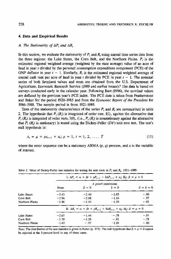
In this section, we evaluate the stationarity of Pt and Rt using annual time series data from the three regions: the Lake States, the Corn Belt, and the Northern Plains. Pt is the estimated regional weighted average (weighted by the state acreage) value of an acre of land in year t divided by the personal consumption expenditure component (PCE) of the GNP deflator in year t - 1. Similarly, Rt is the estimated regional weighted average of annual cash rent per acre of land in year t divided by PCE in year t - 1. The nominal series of both farmland values and rents are obtained from the U.S. Department of Agriculture, Economic Research Service (1989 and earlier issues), s The data is based on surveys conducted early in the calendar year. Following Burt (1986), the nominal values are deflated by the previous year's PCE index. The PCE data is taken from Featherstone and Baker "for the period 1920-1985 and from the Economic Report of the President for 1986-1988. The sample period is from 1921-1989.

Tests of the stationarity characteristics of the series Pt and Rt are summarized in table 2. The hypothesis that Pt (Rt) is integrated of order one, I(1), against the alternative that Pt (Rt) is integrated of order zero, I(0), (i.e., P t (Rt) is nonstationary against the alternative that Pt (Rt) is stationary) is tested using the Dickey-Fuller (DF) unit root test. The test's null hypothesis is:

xt = # + pxt-1 + ut; p = 1, t = 1 ,2 , . . . . T (11)

where the error sequence can be a stationary ARMA (p, q) process, and x is the variable of interest.

Table 2. Value o f D i c k e y - F u U e r test s ta t i s t ics for t es t ing for un i t roots in Pt and Rt, 1 9 2 1 - 1 9 8 9 .

I. AP t = ot + 3t + oPt- I + 6APt-1 + ut; H 0 : 3 = P = 0

A priori r e s t r i c t i ons

N o n e 3 = 0 6 = 0 j3 = 6 = 0

L a k e States - 3 . 4 3 - 2 . 4 0 - 1.05 - . 9 0

C o r n Bel t - 2 . 9 4 - 2 . 0 8 - 1 .14 - .97

N o r t h e r n P la ins - 2 . 8 6 - 2 . 1 3 - 1 .39 - . 9 3

11. AR t = ~ + fit + oRt_ 1 + ~ARt-1 + ut; H0: ~ = P = 0

L a k e States - 2 . 0 7 - 1 .44 - .78 - .91

C o r n Bel t - 1 .70 - 1 .26 - .81 - .78

N o r t h e r n P la ins - 1.43 - . 9 7 - 1 .24 - .80

Note: T h e d i s t r ibu t ion o f the tes t s ta t is t ics is g i v e n in Fu l l e r (p. 373) . T h e nul l hypo the s i s tha t 13 = p = 0 canno t

be re jec ted at the 5 -pe rcen t l eve l in any o f t h e s e cases .


Two versions of the test statistic were applied to the data: DF(/z), which allows for a constant term in the fitted regression; and DF(Iz, t), which allows for a constant term and trend in the fitted regression. Both statistics have equation (11) as their null hypothesis, but possess different critical values. When carrying out the DF(#) test, the null hypothesis is equation (11) with/z = 0. The alternative hypothesis in DF(#) is that the data possesses a stationary autoregressive representation about a constant term, #. For DF(tz, t), the alternative specification implies that the data follows a stable autoregressive model about a constant term and a linear trend.

Both tests, the details of which are given in Dickey and Fuller (1979) and Fuller (1976), are implemented by testing the null hypothesis that/3 = 0 = 0 in a model of the form:

z~kX t = IA "Jv ~t + pxt_ 1 -[- ~ 6 iAx t_ i -[- e t i=1

(12)

where e t is assumed to be distributed N.I.I .D(0, o2). For either test, the test statistic, z, is computed as the ratio of the OLS estimate of p to its standard error. The distribution of this test statistic is discussed in Dickey and Fuller and in Fuller. The critical values for DF(Iz), ~ , and DF(Iz, t), "~, are given in Fuller, p. 373.

An a priori restriction/3 = 0 was imposed on the DF(#) test. Both the DF(tz) and DF(#, t) tests were carried out with and without imposing the restriction 6 = 0. The regressions were run with and without autoregressive terms. The autoregressive terms appear to be necessary to make the errors serially independent.

The rejection region for the five percent test for unit roots includes values smaller (more negative) than - 2 . 9 3 for DF(tz) and -3 .50 for DF(#, t). As can be seen in table 2, in no case were we able to reject the null hypothesis of a unit root in Pt or R t at the .05 level. The results reported in table 2 suggest that Pt and Rt are nonstationary in levels but are stationary in their first differences. 6

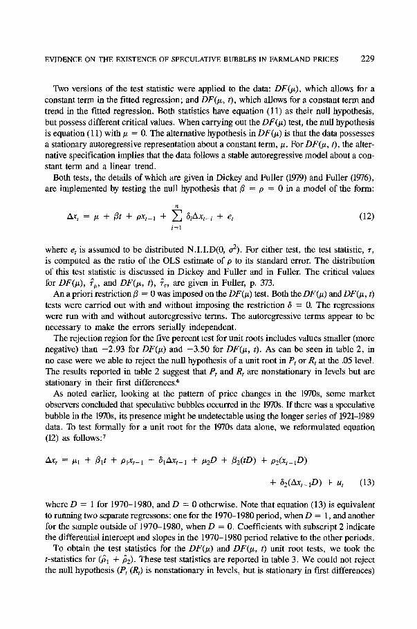
As noted earlier, looking at the pattern of price changes in the 1970s, some market observers concluded that speculative bubbles occurred in the 1970s. I f there was a speculative bubble in the 1970s, its presence might be undetectable using the longer series of 1921-1989 data. To test formally for a unit root for the 1970s data alone, we reformulated equation (12) as follows: 7

z~x t = tzl + 131t + PlXt_l + (~l~t_l q- /z2O -'[- /~2(tD) q- P2(Xt_lD)

+ 62(z~Ct_l D ) + U t (13)

where D = 1 for 1970-1980, and D = 0 otherwise. Note that equation (13) is equivalent to nmning two separate regressons: one for the 1970-1980 period, when D = 1, and another for the sample outside of 1970-1980, when D = 0. Coefficients with subscript 2 indicate the differential intercept and slopes in the 1970-1980 period relative to the other periods.

To obtain the test statistics for the DF(#) and DF(#, t) unit root tests, we took the t-statistics for (ill + 22)- These test statistics are reported in table 3. We could not reject the null hypothesis (Pt (Rt) is nonstationary in levels, but is stationary in first differences)

230 A B E B A Y E H U T E G E N E A N D F R E D E R I C K R. K U C H L E R

Table 3. Value of Dickey-Fuller test statistics for testing for unit roots in Pt and Rt, 1970-1980 .

I. AP t = oq + B t t + ptPt_l + f l ake r - 1 + o~2D + /32(tD) + p2(et_l D) + f2(zM~t_l D ) + ut; H 0 : ~ 1 = ~2 = Ol = P2 = 0

A priori restr ict ions

None fll = /~2 = 0 fit = 62 = 0 /31 = /~2 = f l = 52 = 0

Lake States - 1 .697 1.443 - 1 .267 2 . 3 6 2

Corn Belt - 3 . 1 0 5 1.107 2 . 6 9 9 1 .953

Nor the rn Plains - 3 . 0 0 3 1 .250 2 . 4 0 9 1.79

I I . ~kR I = ~1 "~" 3it + plRt-1 + fl~kR/-I "~ c~2D + 32(tD) + p2(Rt-1D) + f2(ARt_ID) + u,; H0:/31 = /32 = a t = 02 = 0

Lake States - 3 .503 - 1 .155 - 2 . 8 2 0 - . 18

Corn Belt - 3 . 4 7 7 - . 6 0 8 - 3 . 0 6 3 - . 3 0 6

Nor thern Plains -2 .699 - . 7 9 3 - 2 . 5 8 4 - . 8 9 9

Note: The distr ibution o f the test statistics is g iven in Ful ler (p. 373). The null hypothesis that 131 = ~2 = a t

= p: = 0 cannot be rejected at the 10-percent level in any o f these cases .

at the five percent level for any case. In the Lake States (equation for R), ~ is equal to the critical value at the five percent level. In some cases, the test statistics are even the wrong sign for the series to be stationary in levels.

Perron (1989) extended the Dickey-Fuller methodology so that it can be applied to test for a unit root in a time series when there is a one-time change in the structure ("interventions") of the series. The interventions are assumed to occur at a known date, TB (1 <TB < T, where T is the sample size). The approach allows an exogenous change in the level and/or the rate of growth of the series.

The null hypothesis is that the time series is characterized by the presence of a unit root. The approach allows the change in the trend function to be instantaneous or gradual. For a case in which both the level and the trend coefficients are allowed to change gradually, the equation to be estimated is:

k xt = I~ + 13t + pxt-1 + Z ~iAxt-i + OD1 + ,/D2 + c~D3 + e t (14)

/=1

whereD1 = 1, i f t > T~;D2 = t, i f t > TB;andD3 = 1, i f t = TB + 1. The null hypothesis of a unit root is tested using the "t-statistic," tp, t~ divided by its

standard error. Perron tabulated critical values for the distribution of t 0 for testing a unit root in equation (14). The critical values are tabulated for different values of )~ = TB/T.

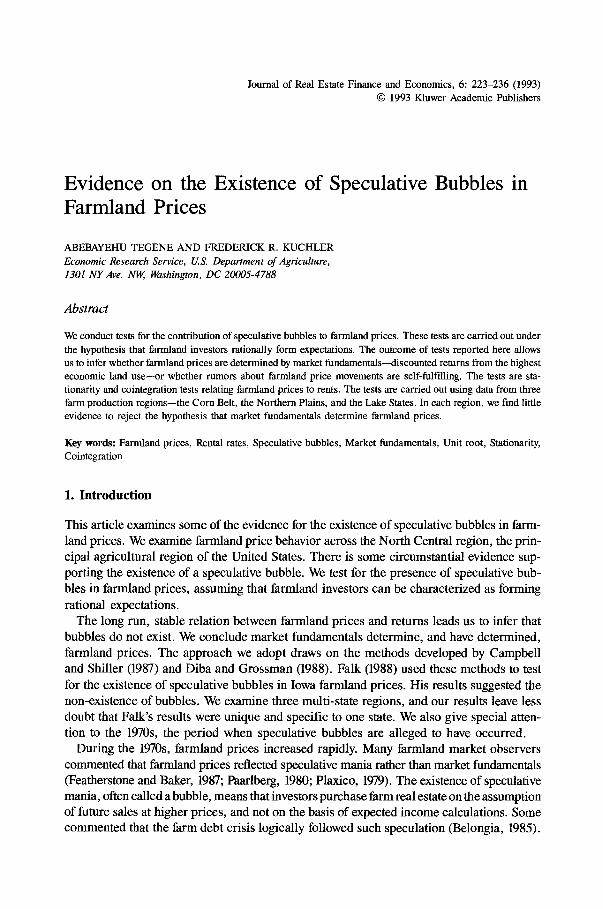
Visual inspection of Figure 1 indicates two significant changes in the trend function of prices and rents: one at the beginning of 1970s and another at the beginning of 1980s. The changes appear to be gradual rather than instantaneous. Since Perron's method deals with one break in the series, and since our main interest is in the 1970s, we ran the test using 1921-1980 data, with the change in the structure of the series assumed to have occurred in 1970 (i.e., TB = 1970). We focus on the development of the bubble.


We ran equation (14) for both the price and rent series for the three regions. The "t- statistics" for testing O = 1 (unit root) with k = 2 were (-2.31, -3.04, -2.02) for the price and ( - 2 . 72 , -1 .77 , -1.53) for the rent series in the Lake States, Corn Belt, and Northern Plains, respectively. Critical values for ~ = .83 (TB/T) are -4 .04 (5 percent) and -3.69 (10 percent) levels (Perron, 1989, p. 1377). The null hypothesis of a unit root cannot be rejected even at the ten percent level in any of the series.

We also carried out the test assuming only the slope of the trend function changes after 1970. The "t-statistics" for k = 2 are ( -2 .89 , -3 .46 , -2 .42) for the price series and (-2.83, -1.79, -1.52) for the rent series in the Lake States, Corn Belt, and Northern Plains, respectively. Critical values are -3.82 (5 percent level) and -3.50 (ten percent level). Again, we fail to reject the presence of unit root in each of the series.

The results obtained from Perron's test and Dickey-Fuller tests (tables 2 and 3) suggest that the farmland values and rents in each of the three regions are integrated of order one. First order integration implies that AP t and ARt are stationary. One implication of the "spread" model shown in equations 9, 9a, and 10 is that if A R t is a stationary series, then the present value model implies that APt will also be stationary in the absence of rational bubbles. The results presented above provide no evidence for the presence of a rational bubble in farmland prices. In the next section, we examine another implication of the spread model.

B. Cointegration o f Pt and R e

The second implication of the model of price "spread" is the positive proposition that prices and rents must be cointegrated. The notion of cointegration corresponds to the notion of long run equilibrium. Consider for example, a pair of series xt and Yt each of which is I (d) . The linear combination zt = xt - otyt will generally be I(d). However, if there is a constant ot such that zt is I (d - b), where b > 0, xt and Yt are said to be cointegrated of order d, b (CI(d, b)), and the vector (1, -or) is called the cointegrating vector and the relation x t = otyt is called the cointegrating regression (Granger, 1986; Engle and Granger, 1987). Integration of the same order is a necessary (but not sufficient) condition for a pair of variables to be cointegrated. There are two cointegrating regressons: xt on Yt and Yt on xt. Stock (1987) has shown that a consistent estimator of ot can be obtained from the regression of xt on Yt and also from the inverse regression coefficient of Yt on xt.

The relation xt = otyt may be considered a long run or equilibrium relationship and zt

measures the extent to which the system composed of xt and Yt is out of equilibrium. If xt and Yt are I(1) but move together in the long run, their difference (sometimes denoted equilibrium error), zt, will be I(0). Otherwise, the two series will drift apart without bound (Granger, 1986). Hence, cointegration of a pair of variables is at least a necessary condition for the variables to display a stable, long run relation.

Applying the Campbell and Shiller argument to the farmland price example indicates if (1) the first differences of rents (ARt) are stationary, and (2) rational bubbles do not exist, then farmland values and rents are cointegrated of order (1, 1), (Falk, 1988). That is, evidence that first differences of prices and rents are stationary and/or evidence that prices and rents are cointegrated would be evidence against the existence of a rational bubble


(Diba and Grossman, 1988). The converse hypothesis is, however, not verified by nonsta- tionarity findings or by failure to demonstrate cointegration? The finding that first differences of farmland prices and rents are nonstationary, or that prices and rents are not cointegrated, will not necessarily establish the existence of a rational bubble.

In the preceding section, we found evidence that farmland price changes in all three regions are stationary. In this section, we examine whether or not farmland prices are cointegrated with rents. A number of tests have been proposed recently to determine if a pair of series xt and Yt are cointegrated. 9 Engle and Granger (1987) have computed the critical values and examined the power properties of the various tests. In a first order system, two procedures, Durbin-Watson and Dickey-Fuller tests, were found to be most powerful. For higher order systems, Engle and Granger recommended the Augmented Dickey-Fuller (ADF) test.

The ADF cointegration test null hypothesis is H0: xt and Yt are not cointegrated. The test statistic is computed from results of two regression equations. The cointegration regression of xt on Yt yields OLS residuals denoted Ur The regression

n

AUt = I ~ + f~O Ut-1 "-]- E ~ iAut - i "[- Yt i=1

(16)

yields the test statistic, the ratio of/~0 to its estimated standard error. The order of n is set to ensure that the estimated residuals series, vt, is white noise.

Given the empirical evidence above that the farmland price and rent series in each region is I(1), for the price and the rent series to be cointegrated, the spread as defined by equation (8) must be I(0). This latter condition implies the absence of an explosive rational bubble in farmland prices. That is, in the absence of a rational bubble, land prices and rents will be CI(1, 1) with cointegrating vector (1, - r - l ) .

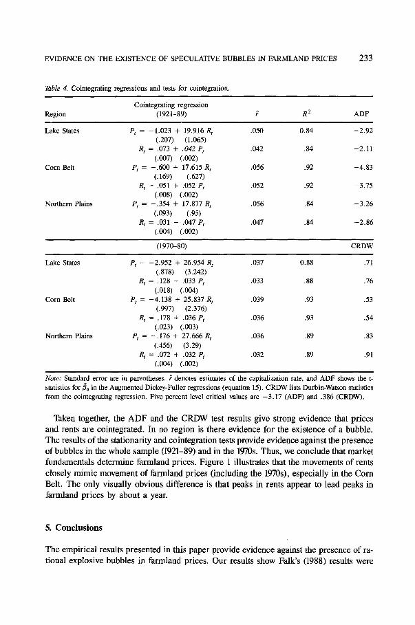
Table 4 presents the cointegration regressions and the summary of the results of cointegration tests between Pt and R t. The cointegrating regressions were run in both directions. The upper half of the table shows the results of the ADF test using the 1921-1989 data. Critical values for ADF cointegration test are -2.84, -3.17, and -3 .77 at the 10 percent, 5 percent, and 1 percent level, respectively (Engle and Granger, 1987, p. 269). The hypothesis of no cointegration between farmland prices and rents is rejected at the one percent level in the Corn Belt and the Northern Plains regions (when R t is the regressor) and at the ten percent level in the Lake States (when Rt is the regressor). The hypothesis could not be rejected for the Lake States at the ten percent level when Pt is the regressor. The less conclusive result for the Lake States could be due to the low power of these tests. Thus, we conclude there is very strong evidence that farmland prices and rents are cointegrated in two regions and there is weak evidence for cointegration in the Lake States.

With only 11 observations, we could not use the ADF test of cointegration for the 1970-1980 data. Since the cointegrating regression Durbin-Watson (CRDW) test leaves larger degrees of freedom than the ADF or DF tests, we used the CRDW test for this segment of the sample. The results are shown in the second panel of table 4. The DW statistic for the cointegration regression is larger :than .511 in every case. At the one percent level, the staistics imply we should reject the hypothesis of non-cointegration between Pt and R t in the 1970s. Although the sample size is very limited, the results do suggest that prices and rents are cointegrated.


Table 4. Cointegrating regressions and tests for cointegration.

Cointegrating regression Region (1921-89) ~ R 2 ADF

Lake States Pt = - 1.023 + 19.916 R t .050 0.84 -2.92 (.207) (1.065)

R t = .073 + .042 Pt .042 .84 -2.11 (.007) (.002)

Corn Belt Pt = -.600 + 17.615 R t .056 .92 -4.83 (.169) (.627)

R t = .051 + .052 Pt .052 .92 -3.75 (.008) (.002)

Northern Plains Pt = -.354 + 17.877 R t .056 .84 -3.26 (.093) (.95)

R t = .031 + .047 Pt .047 .84 -2.86 (.004) (.002)

(1970-80) CRDW

Lake States Pt = -2.952 + 26.954 R t .037 0.88 .71 (.878) (3.242)

R t = .128 + .033 Pt .033 .88 .76 (.018) (.004)

Corn Belt Pt = -4.138 + 25.837 R t .039 .93 .53 (.997) (2.376)

R t = .178 + .036 Pt .036 .93 .54 (.023) (.003)

Northern Plains Pt = -.176 + 27.666 R t .036 .89 .83 (.456) (3.29)

R t = .072 + .032 Pt .032 .89 .91 (.004) (.002)

Note: Standard error are in parentheses. ~ denotes estimates of the capitalization rate, and ADF shows the t- statistics for rio in the Augmented Dickey-Fuller regressions (equation 15). CRDW lists Durbin-Watson statistics from the cointegrating regression. Five percent level critical values are -3.17 (ADF) and .386 (CRDW).

Taken together, the A D F and the C R D W test results g ive strong ev idence that pr ices

and rents a re cointegrated. In no reg ion is there ev idence for the existence o f a bubble.

The results o f the stationarity and cointegrat ion tests provide evidence against the presence

of bubbles in the whole sample (1921-89) and in the 1970s. Thus, we conclude that market

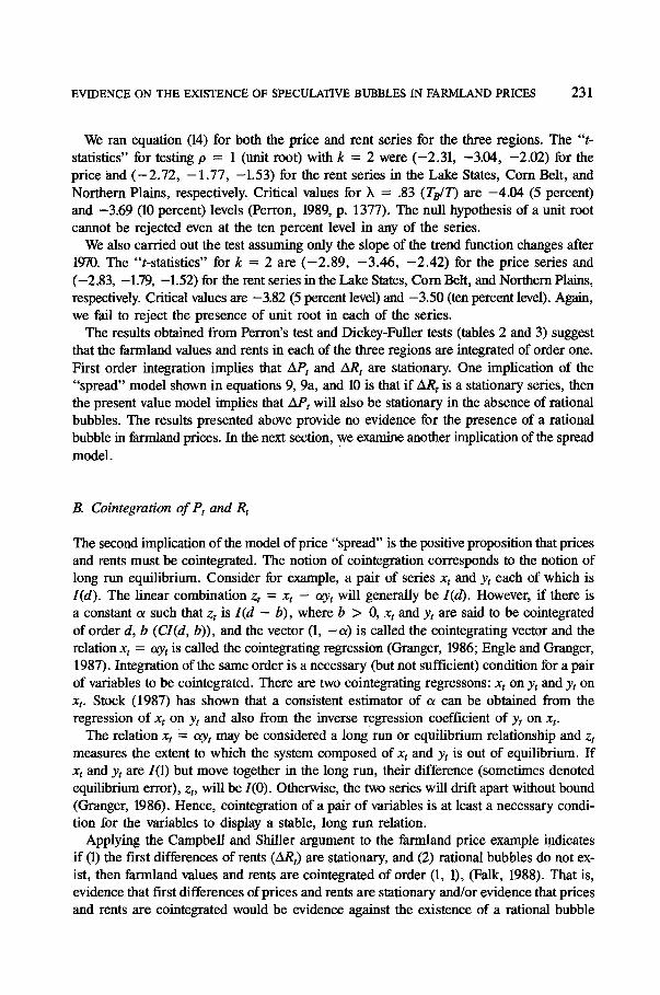
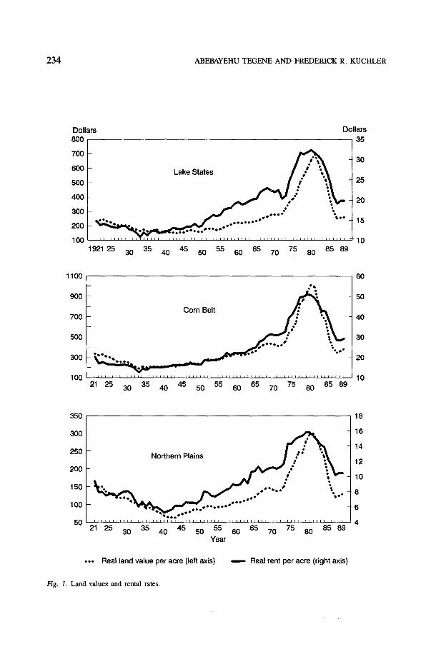
fundamentals de termine farmland prices. F igure 1 il lustrates that the movements of rents

c losely m i m i c m o v e m e n t o f farmland prices ( including the 1970s), especial ly in the Corn

Belt. The only visual ly obvious di f ference is that peaks in rents appear to lead peaks in

farmland pr ices by about a year.

5. Conclusions

The empi r ica l results presented in this paper provide ev idence against the presence of ra-

t ional explos ive bubbles in farmland prices. Our results show Falk 's (1988) results were

2 3 4 ABEBAYEHU TEGENE AND FREDERICK R. KUCHLER

Dollars 800

Dollars 35

700

600

500

400

300

200

100

Lake States

. . . . . . �9 ' ' " ~ , . . - .~ ~.." ~eeQe~ ~ ,oe ~176176176176

oee~ ~176 t1111;111111 i ~ l l l l l l = l l l l t l l l = i l t l l l i = l q l l i = l l = l l i i l l l ~ i i l i l t l l i t l l ~

1921 25 30 35 40 45 50 55 60 65 70 75 80 85 89

30

25

20

15

10

1100 60

900 ~ 50

Corn Belt 700 40

500 30 ~ v -%,o oQe ~ ~ 1 7 6 ~ ' ~

300 20

100 10 21 25 30 35 40 45 50 55 60 65 70 75 80 85 89

350 [- . . . . . . . . . . . . . . . 18

250 14 200 Northern Plains = 12

150 �9 " % �9 o ~oe 8

~176 . . . . t . . . . 0 . . . ~ -~ 6 50 ; l l l l l l l l l l r l l l l ~ l l t l l l l L i i I I I l ~ l T I I l l l ~ l l l l l ~ l l l ~ l ~ l l l l l l l l ~ l l l l l l l 4

21 25 35 45 55 65 75 85 89 30 40 50 60 70 80 Year

�9 .. Real land value per acre (left axis) ~ , - Real rent per acre (right axis)

F/g. 1. Land values and rental rates.


not anomalous. Further, examination of the 1970-1980 data alone do not show any evidence for the existence of speculative bubbles. If there was no speculative bubble, then one must conclude that the run up in farmland prices during the 1970s was the result of changed expectations.

There are many ways expectations could have changed, causing farmland prices to rise. In the 1970s, farmland investors may have believed that income from farming would rise. Alternatively, the low real interest rates might have caused investors to believe that they ought to reduce the rate at which they discount future income.

Many analysts have stated that the aggressive lending policies of the Farm Credit System touched off a speculative bubble in farmland prices. That conclusion appears to be incor- rect, but the evidence does not rule out the possibility that aggressive lending, reflected in lower mortgage rates, could have caused investors to re-evaluate their expectations.

With real exports growing more than 10 percent a year in the 1970s, many analysts and policymakers expressed concern that farmers worldwide could not produce enough food and that demand for U.S. agricultural products would keep rising. But U.S. agricultural exports declined by more than 50 percent from their peak during the early 1980s, showing that forecasts of slow food production growth relative to demand were wrong.

The Federal Reserve changed its operating procedures from targeting interest rates to limiting money growth in 1979 and sharply cut the inflation rate in the early 1980s. Growth in worldwide agriculture production, a global recession, a higher dollar, and steeply rising real interest rates have been credited with pushing U.S. agriculture into its most severe financial crisis since the Great Depresssion.

The quadrupling of farmland prices in some regions during the 1970s ought not to be surprising. Many factors changed. Instead of evidence for a speculative bubble, the price changes could indicate that investors use forecasts cautiously in their business planning.

Notes

1. See U.S. Department of Agriculture, Economic Research Service (1989). In 1988, for example, close to 50 percent of the land operated in these regions was rented.

2. Although cash rents are not a perfect measure of land earnings, they are found to predict land price changes much more accurately than does farm income (Tweeten, 1986) and are major determinants of land values (Castle and Hoch, 1982; Burt, 1986).

3. Burt (1986) argues that a constant real interest rate is appropriate for modelling farmland prices. 4. "The rate of return to land on a current account basis (current income/current price) has ranged from 3%

to 5 %." (Scott, 1983, p. 796). 5. See Tegene and Kuchler (1990) for details of data construction. 6. All values of the DF(tt) and DF(#, t) for testing AP t (ARt) is stationary exceed the critical value, -3.50. We

also applied Hasza-Fuller tests to test the null hypothesis that Pt (Rt) is I(2) against the alternative hypothesis that Pt(Rt) is I(0) or 1(1). The results were consistent with the conclusion that Pt and R t are nonstationary in levels, but are stationary in first differences. The details of these tests are available from the authors.

7. Although the sample is too small to derive any reliable inference, we nonetheless computed the DF~) statistics using eleven observations (1970-1980). In each of the six cases, ~:u, was positive.

8. For example, the presence of a nonstationary unobservable component in market fundamentals could make prices and rents non-cointegrated (Diba and Grossman, 1988).

9. Useful summaries are provided in Engle and Granger 0987).


References

Belongia, M.T. "Factors Behind the Rise and Fall of Farmland Prices: A Preliminary Assessment?' Fed. Res. Bank of St. Louis Rev. 67 (1985), 18-24.

Blanchard, O.J., and Fischer, S., Lectures on Macroeconomics. Cambridge: MIT Press, 1989. Blanchard, O.J., and Watson, M. "Bubbles, Rational Expectations and Financial Markets" In P. Wachtel, ed.,

Crisis in the Economic and Financial Structure. Lexington: Lexington Books, 1982. Burt, O.R. "Econometric Modeling of the Capitalization Formula for Farmland Prices)' American Journal of

Agricultural Economics 68 (1986), 10-26. Campbell, J., and ShiUer, R, "Cointegration, and Tests of the Present Value Relation" Journal of Political Economy

95 (1987), 1062-1088. Castle, E.N., and Hoch, I. "Farm Real Estate Price Components, 1920-19787' American Journal of Agricultural

Economics 64 (1982), 8-18. Diba, B.T. "Bubbles and Stuck-Price Volatility." In G.P. Dwyer and R.W. Haler, eels., The Stock Market: Bub-

bles, Volatility, and Chaos, Boston: Kluwer Academic Publishers, 1990. Diba, B., and Grossman, H. "Explosive Rational Bubbles in Stock Prices?" American Economic Review 78 (1988),

520-30. Dickey, D., and Fuller, W. "Distribution of the Estimators for Autoregressive Time Series with a Unit Root?'

Journal of the American Statistical Association 74 (1979), 427-31. Engle, R., and Granger, C.W.J. "Cointegration and Error-Correction: Representation, Estimation, and Testing?'

Econometrica 55 (1987) 251-76. Falk, B. '~A Search for Speculative Bubbles in Farmland Prices?' Department of Economics working paper, Iowa

State University, 1988. Featherstone, A.M., and Baker, T. ' ~n Examination of Farm Sector Real Asset Dynamics: 1910-85." American

Journal of Agricultural Economics 69 (1987), 532-546. Flood, R.P., and Hodrick, R.J. "On Testing for Speculative Bubbles?' Journal of Economic Perspectives 4 (1990),

85-101. Fuller, W. Introduction to Statistical "l~me Series. New York: Wiley, 1976. Granger, C.W.J. "Developments in the Study of Cointegrated Economic Variables)' Oxford Bulletin of Economics

and Statistics 48 (1986), 213-218. Paarlberg, D. Farm and Food Policy Issues of the 1980's. Lincoln: University of Nebraska Press, 1980. Perron, P. "The Great Crash, the Oil Price Shock, and the Unit Root Hypothesis." Econometrica 57 (1989),

1361-1401. Plaxico, J.S. "Implications of Divergences in Sources of Returns in Agriculture" American Journal of Agricultural

Economics 61 (1979), 1098-1102. Scott, Jr., J.T. "Factors Affecting Land Price Decline." American Journal of Agricultural Economics 83 (1983),

796-800. Stock, J. '9~symptotic Properties of Least Squares Estimators of Cointegration Vectors)' Econometrica 55 (1987),

1035-56. Taylor, J.B. "On the Conditions of Uniqueness in the Solution of Rational Expectations Models?' Econometrica

45 (1977), 1377-85. Tegene, A. and Kuchler, E "The Contribution of Speculative Bubbles to Farmland Prices)' Tech. Bul. No. 1782

U.S. Depa~ment of Agriculture, Economic Research Service, July 1990. Tweeten, L. 'gt Note on Explaining Farmland Price Changes in the Seventies and Eighties" Agricultural Economics

Research 38 (1986), 25-30. U.S. Department of Agriculture, Economic Reseach Service. '~gricultural Resources: Agricultural Land Values

and Market Situation and Outlook Report?' AR-18, Washington, D.C. (June 1989). West, K. "A Specification Test for Speculative Bubbles?' Quarterly Journal of Economics 102 (198"/), 553-580.

Documents

Evidence on the existence of speculative bubbles in farmland prices