Fe

dera

l Res

erve

Ban

k of

Chi

cago

A Leverage-based Model of Speculative Bubbles

Gadi Barlevy

REVISED July 8, 2013 WP 2011-07

A Leverage-based Model of Speculative Bubbles∗

Gadi BarlevyEconomic Research DepartmentFederal Reserve Bank of Chicago

230 South LaSalleChicago, IL 60604

e-mail: gbarlevy@frbchi.org

July 8, 2013

Abstract

This paper examines whether theoretical models of bubbles based on the notion that the price ofan asset can deviate from its fundamental value are useful for understanding historical episodes thatare often described as bubbles, and which are distinguished by features such as asset price boomsand busts, speculative trading, and seemingly easy credit terms. In particular, I focus on risk-shiftingmodels similar to those developed in Allen and Gorton (1993) and Allen and Gale (2000). I show thatsuch models could give rise to these phenomena, and discuss under what conditions price booms andspeculative trading would emerge. In addition, I show that these models imply that speculative bubblescan be associated with low spreads between borrowing rates and the risk free rate, in accordance withobservations on credit conditions during historical episodes often suspected to be bubbles.

∗This paper represents a substantial revision of Federal Reserve Bank of Chicago Working paper No. 2008-01. I am gratefulto Franklin Allen, Marios Angeletos, Bob Barsky, Marco Bassetto, Christian Hellwig, Guido Lorenzoni, Kiminori Matsuyama,Ezra Oberfield, Rob Shimer, Kjetil Storesletten, and Venky Venkateswaran for helpful discussions, as well as participants atvarious seminars. I also wish to thank David Miller, Kenley Barrett, and Shani Shechter for their research assistance on thisor earlier versions of the paper. The views expressed here need not reflect those of the Federal Reserve Bank of Chicago or theFederal Reserve System.

1

1 Introduction

The large fluctuations in U.S. equity and housing prices over the past decade and a half have led to renewed

interest in the phenomenon of asset bubbles. Among non-economists, the term “bubble”has come to refer

to any historical episode in which asset prices rise and fall significantly over a relatively short period of

time.1 By contrast, economists usually use the term “bubble”to mean that an asset trades at a price that

differs from its fundamental value, i.e. the expected discounted value of the dividends it generates. The

latter notion is meant to capture the idea that asset prices convey distorted signals as to the true value

of the underlying assets. The two notions are certainly compatible: The price of an asset can rise above

fundamentals and then collapse. But economists working on models of bubbles have largely ignored the

question of whether these models can account for the key features of the historical episodes suspected to

be bubbles, focusing instead on whether assets can trade at a price that differs from fundamentals. The

distinguishing features of the historical episodes include not just a boom and bust in asset prices, but a high

incidence of speculative trading in which agents buy assets with the explicit aim of profiting from selling

them later on rather than accruing dividends and low spreads on loans taken out against these assets.

This paper examines whether one particular class of models that can generate a gap between the price of an

asset and its fundamental value —the risk-shifting theory of bubbles developed by Allen and Gorton (1993)

and Allen and Gale (2000) —can also generate the qualitative features common to the historical episodes

often described as bubbles. In risk-shifting models, traders purchase risky assets with funds obtained from

others. The financial contracts traders use to secure these funds are assumed to involve limited liability.

The latter feature implies traders would be willing to pay more for assets than the expected dividends they

yield, since traders can shift any losses they incur on to their financiers. In other words, agents value assets

above the dividends these assets generate because of the option to default on loans issued against the asset.

This intuition can be illustrated in a purely static model where assets trade hands exactly once. Thus,

overvaluation can occur independently of boom-bust dynamics or speculative trade.

While both Allen and Gorton (1993) and Allen and Gale (2000) consider dynamic models of risk-shifting,

the various assumptions they impose to maintain tractability make it diffi cult to gauge whether and when

these models give rise to the key features that characterize the historical episodes often described as “bub-

bles.”For example, Allen and Gorton (1993) assume bilateral trades rather than a market for assets. This

implies asset prices in their model are not uniquely determined, and so their model has little to say on when

price booms and busts will arise. In addition, both papers effectively require agents who buy an overvalued

asset to sell it after some exogenously determined holding period. As such, they cannot address whether

1For example, Merriam-Webster.com defines a bubble as “a state of booming economic activity (as in a stock market) thatoften ends in a sudden collapse,”while the New York Times Online Guide to Essential Knowledge defines it as a “market inwhich the price of an asset continues to rise because speculators believe it will continue to rise even further, until prices reacha level that is not sustainable; panic selling begins and the price falls precipitously.”

1

these models give rise to “speculative”bubbles in which traders buy an asset with the aim of profiting from

selling it, or to what Hong and Sraer (2011) dub “quiet”bubbles in which assets are overvalued but trade

only infrequently. To address these questions requires a dynamic model in which agents trade strategically.

There has also been little work on whether risk-shifting models of bubbles are consistent with the lax

credit conditions that accompany historical episodes identified as bubbles. At a first glance, these models

seem to imply that if anything, bubbles should be associated with higher borrowing costs. In particular,

traders who buy overvalued assets are only able to raise funds by pooling with other borrowers whom

financiers would like to finance. If creditors understand that some of those they fund will buy risky assets,

they would presumably charge a spread over the risk-free rate to cover the expected losses on speculators.

One of the points of this paper is to show why this intuition can be misleading, and to outline reasons why

the spread between the borrowing rate and the risk-free rate may in fact be lower in speculative episodes.

In what follows, I develop a dynamic model of risk-shifting where agents borrow to buy risky assets and

then choose if and when to sell them. If agents fear that future traders may not always buy the asset in

order to gamble at the expense of creditors, assets can exhibit rapid price appreciation as long as they

continue to trade. The intuition is related to the one Blanchard and Watson (1982) derive for rational

bubbles: If an asset might cease to become overvalued in the future, rational agents must be compensated

for holding the asset now while it is still overvalued rather than sell it. This compensation accrues as

capital gains if the asset remains overvalued. However, an important difference between the Blanchard and

Watson (1982) framework and mine is that their model is silent on whether assets trade, since agents in

their model are always indifferent between holding and selling an asset. This is not true in my model, where

agents sometimes sell the asset and sometimes hold it to maturity. This feature of my model reveals that

the price dynamics in Blanchard and Watson (1982) should be seen as a bound on the rate of asset price

appreciation rather than the rate at which rational bubbles always grow. It also reveals when bubbles will

be “noisy” rather than quiet and feature repeated trade: When assets are more overvalued, when asset

price appreciation is high, and when assets returns are skewed towards a high upside potential relative to

the mean. An additional insight is that noisy bubbles can be associated with lower borrowing spreads than

quiet bubbles. This is because when traders sell bubble assets, the risk lenders are exposed to in lending

against assets is partly shifted to future lenders. Thus, it may be cheap to borrow against assets precisely

when assets trade hands repeatedly, a common feature of empirical episodes suspected to be bubbles.

The second modification I consider is to allow lenders to design contracts optimally. This modification

reveals another reason why speculation can be associated with low borrowing spreads, especially for specu-

lators. Specifically, lenders will want to minimize the losses they incur from speculators, e.g. by restricting

loan size or providing only short-term financing. At the same time, lenders would not want to impose these

features on profitable borrowers. To induce speculators to accept more restricted contracts, lenders must

make them more attractive on some other dimension, which can include lower rates.

2

While this paper only considers risk-shifting models of bubbles, other models have been developed in

which assets can trade above their fundamental value. One example are models in which there is a shortage

of assets that perform some essential function such as a store of value or liquidity. This scarcity can lead

people to value whatever assets are available above and beyond the dividends they yield. Examples of

such models include overlapping generations models such as Samuelson (1958), Diamond (1965), and Tirole

(1985).2 Another example are the so-called “greater-fool” models of bubbles, where agents buy assets

they view as overvalued because they expect to profitably resell these assets to other agents who value the

asset differently. These models include Allen, Morris, and Postlewaite (1993) and Conlon (2004). Without

denying the importance of these models, there does seem to be value in studying risk-shifting models of

bubbles in particular. One reason is that in these models credit markets play a central role in allowing

bubbles to arise, which accords with the observation that in many historical episodes traders would often

borrow against the assets they purchase. The central role of credit markets also implies these models can be

used to explore one potential concern about bubbles, namely that the collapse of a bubble can be especially

consequential if it results in default by those who borrowed against these assets. Finally, risk-shifting models

of bubbles can lead to different policy implications than alternative models that give rise to bubbles. For

example, since bubbles do not arise in these models because assets play a valuable role such as a store of

value of liquidity, assets that trade above fundamentals may be ineffi ciently oversupplied. At the same time,

unlike in greater fool models, risk-shifting models allow for it to be common knowledge that some assets

are overpriced, so a policymaker with no more knowledge than private agents might want to intervene.

The paper is structured as follows. Section 2 lays out the basic features of my model economy. Section 3

studies the implications of the model for price dynamics and speculation when the set of contracts agents

can enter is exogenously restricted to simple debt contracts. Section 4 allows for endogenous contracting,

and examines what type of contracts will be offered when speculative bubbles arise. Section 5 concludes.

2 Setup

I begin by describing the key features of the environment I study. The model is meant to generalize the

Allen and Gale (2000) model to allow for strategic dynamic trades and, later on, for endogenous contracting.

To keep the analysis tractable, I restrict attention to a two-period model, where periods are indexed by

t ∈ {1, 2}. I first describe the assets that agents can trade. I then describe the agents who populate the

2There are also examples of such models where agents have infinite horizons, e.g. Kocherlakota (1992) and Santos andWoodford (1997). Both offer examples of bubbles in models inspired by Bewley (1980) where there are finitely many agentswith infinite horizons but limits on what agents can trade. Both papers go on to show that if agents face borrowing limits,bubbles can also emerge on assets available in zero net supply. The latter seems less relevant for understanding historicalepisodes suspected to be bubbles, where the relevant assets were in positive net supply. While early models focused on thecase where assets served the role as a store of value, more recent work, including Caballero and Krishnamurthy (2006), Farhiand Tirole (2011), and Rocheteau and Wright (2011) instead focus on the case where assets provide a liquidity role.

3

economy. Finally, I describe the operation of credit markets in my economy.

As in Allen and Gale (2000), I assume a continuum of assets that are available in fixed supply and cannot

be sold short. Restricting supply in some manner is necessary for assets to trade above their fundamental

value. More generally, I could have allowed for an upward sloping supply schedule within a period, although

this would have been more cumbersome. The fixed supply of the asset can be viewed as a technological

constraint on the production of additional assets. The restrictions on short sales can be motivated by similar

informational frictions to those I consider, e.g. agents who sell short cannot be trusted to deliver the assets

they sell or to replicate its payoffs. However, in what follows I take short sales restrictions as given rather

than derive them. Since the supply of assets is assumed to be fixed, I can normalize its mass to 1.

The payouts on assets are risky. For simplicity, suppose the assets pay a single common dividend d at

the end of date t = 2 that can take on just two values:

d =

{D > 0 with probability ε0 with probability 1− ε (1)

For example, an asset can represent a claim to the profits of a firm with a patent that may or may not pan

out, and D represents the value of profits to the firm if the patent is successful.

At the beginning of date 1, agents know only that d is distributed according to (1). For reasons I explain

shortly, I allow d to be revealed with some probability between dates 1 and 2. That is, before agents trade

the asset at date 2, d will be revealed with probability q ∈ [0, 1]. For example, sticking to the patentexample, a technological discovery may occur at the end of date 1 that reveals whether the patent is viable.

Formally, let It denote the information traders observe at date t concerning dividends. Then I1 = ∅ and

I2 ={

d with probability q∅ with probability 1− q

When 0 < q < 1, agents who buy assets at date 1 are uncertain whether these assets will remain risky at

date 2. This turns out to be important, since the riskiness of the asset affects demand for it, and so demand

for the assets at date 2 is uncertain as of date 1. There are other reasons why demand for the asset might be

uncertain, e.g. the number of agents who show up at date 2 might be random, or there might be uncertainty

as to other assets agents may buy at date 2. I focus on early revelation of d only for convenience.

For simplicity, I will assume agents are all risk neutral and do not discount. As such, the expected utility

value of the dividends the asset generates for any agent is just E [d|It]. I will refer to this expectation asthe fundamental value of the asset. It represents the value to society of creating an additional unit of the

asset at date t. That is, if additional units of the asset could be produced at some cost at date t, the price

of the asset would have to equal E [d|It] to provide proper incentives for creating additional units.

4

I now turn to the agents that populate the economy. Since there are several types of agents in the model,

differing in their endowments and opportunity sets, it will help to begin with a brief overview. At the core of

the model are two types who stand to gain by trading with each other, although this trade does not involve

the assets just described. Rather, some agents, whom I call creditors, are endowed with resources but can

earn only low returns on their savings, while other agents, whom I call entrepreneurs, lack resources but

have access to a production technology that yields a high rate of return. Creditors can thus benefit from

lending to entrepreneurs in exchange for a higher return. The reason these two types have any bearing on

the assets just described is that there is a third group of agents, whom I call non-entrepreneurs, that lack

both resources and access to a production technology, but who can buy the aforementioned risky assets.

If creditors cannot distinguish entrepreneurs from non-entrepreneurs, in trying to trade with entrepreneurs

they may end up lending to non-entrepreneurs who buy risky assets. The desire by creditors to trade with

entrepreneurs allows resources to flow into the asset market and influence asset prices.

Closing the model requires two additional groups: The first group, whom I call original owners, is

endowed with the risky assets at the beginning of date 1. The second group, whom I call non-participants,

lacks resources, lacks access to a productive technology, and cannot trade assets. This group will only

become relevant when I consider endogenous contracts in the next section, where their presence serves

to limit the type of contracts creditors offer. In particular, their presence prevents creditors from paying

non-entrepreneurs not to buy assets, since this would also draw in non-participants who cannot buy assets.

Formally, the endowments and opportunity sets of the five types can be characterized as follows:

1. Creditors: Creditors are endowed with a large amount of resources at date 1 that they can store

until date 2 at a gross return of 1. They can also buy risky assets, although they will never strictly

prefer to do so in equilibrium. The mass of creditors is assumed to be large, more than enough to

supply the demand of potential borrowers whom I discuss next.

2. Entrepreneurs: Entrepreneurs are endowed with neither resources nor assets. However, they have

access to a productive technology that allows them to produce R > 1 units of output per unit of input

invested, up to a capacity of 1 unit of input. I assume they cannot buy risky assets. This avoids

having to verify that they prefer production over buying assets, although there are parameters that

guarantee this will be the case. Entrepreneurs arrive at exogenously set times, either at t = 1 or t = 2,

and if they want to invest they must contact creditors the period they arrive. Regardless of when they

invest, the output from their investment accrues at the end of date 2.

3. Non-Entrepreneurs: Non-entrepreneurs are also endowed with neither resources nor assets. In

contrast to entrepreneurs, they do not have access to a productive technology. But they can buy

risky assets. Like entrepreneurs, they arrive at exogenously set times, either at t = 1 or t = 2, and if

5

they wish to buy risky assets they must both contact creditors and buy assets the period they arrive.

Let nt < ∞ denote the mass of non-entrepreneurs who arrive at date t, and let mt < ∞ denote the

combined mass of entrepreneurs and non-entrepreneurs who arrive at date t. To cut down on the

number of parameters, I assume the ratio of non-entrepreneurs to entrepreneurs is the same in both

periods. That is, regardless of t, the number of non-entrepreneurs nt = φmt for some φ ∈ (0, 1).

4. Original Owners: Original owners are endowed with one unit of the asset each and a large amount

of resources, which they can store at a gross return of 1. For ease of exposition, I assume that unlike

creditors, they do not participate in the credit market, either as lenders or borrowers. This assumption

is not restrictive given that in equilibrium they could not profit from trading in the credit market.

5. Non-Participants: Non-participants are endowed with neither resources, assets, nor a productive

technology. In addition, they face a prohibitive cost of entering the market for risky assets. The mass

of such agents is large, in a sense that will be clarified in Section 4 when they become relevant.

Many of the assumptions above only serve to simplify the analysis, and can be considerably relaxed

without affecting some of the key results. In particular, the result that assets can trade above their funda-

mental value E [d|It] arises because creditors can profitably finance entrepreneurs, but only on terms thatwould make it profitable for non-entrepreneurs to borrow and buy risky assets. The existence of bubbles

thus hinges on there being at least some entrepreneurs with profitable investment opportunities but limited

resources, allowing non-entrepreneurs to borrow and then buy risky assets with little of their own at stake.

The remaining assumptions I impose —such as the exogenous arrival dates of agents, the finite number of

agents who arrive at each period, and the finite capacity of entrepreneurs —are unnecessary for this result.

At the same time, my assumptions do matter for price dynamics and trade volume. Specifically, if there

were no limit on how much agents could borrow at date 1, asset prices would be bid up immediately, assets

would trade hands only once, and asset prices would not grow. To generate price appreciation and repeated

trading, we need total borrowing at date 1 to be finite, so the finite capacity of entrepreneurs is important.

Similarly, assuming that agents arrive at exogenous dates is not entirely innocuous. If entrepreneurs and

non-entrepreneurs all arrived in period 1 and chose when to trade, the number of agents who trade in each

period would be endogenous. Since my results depend on the number of traders that arrive at each period,

it is not obvious that endogenous timing would accommodate all of the phenomena I emphasize. However,

as will become clear below, for certain parameter values such as a small ε, price appreciation and repeated

turnover would probably arise even if I allowed agents to time their actions.

To focus on the key features of the model I am after, I impose two parameter restrictions. First, I restrict

the return on production R to an intermediate range of values:

1 +φ (1− ε)

1− φ (1− ε) < R <1

ε(2)

6

It is easy to verify that this range is nonempty for φ ∈ (0, 1) and ε ∈ (0, 1). The reason R cannot be too lowis that the earnings of entrepreneurs must cover the expected losses creditors incur on non-entrepreneurs

who use the funds they borrow to buy risky assets. At low values of R, lending would simply shut down. But

high values of R can also be problematic. In particular, if R exceeded 1/ε, entrepreneurs would earn a higher

return than non-entrepreneurs could ever earn from buying risky assets. This implies non-entrepreneurs

might not be able to profit from buying risky assets, since borrowers may be charged a high rate that still

attracts entrepreneurs but would make it unprofitable to buy and hold risky assets. In addition, once I allow

more general contracts, if entrepreneurs earn more than non-entrepreneurs ever could they could prove their

type to creditors by showing their earnings. Creditors could then avoid lending to non-entrepreneurs.

Second, I restrict the total number of non-entrepreneurs over the two periods to not be too large:

n1 + n2 < (1− q)D/R+ qεD (3)

Since each agent will be able to borrow at most one unit of resources given the finite capacity of entrepre-

neurs, assumption (3) restricts the total amount of resources agents can borrow to spend on risky assets.

As we shall see below, this will impose an upper bound on the price of the asset. (3) rules out the case

where the price of the asset is high enough that non-entrepreneurs who buy risky assets earn zero expected

profits, rendering them indifferent between buying and not buying the asset. The latter case introduces an

additional variable —the fraction of non-entrepreneurs who buy assets —and is thus more tedious to analyze.

Remark 1: Note that the second inequality in (2) implies D/R > εD. Hence, the upper bound in (3) is

strictly greater than εD for q < 1. In the next section I show that n1+n2 > εD is a necessary and suffi cient

condition for a bubble. My parametric restrictions are thus compatible with the possibility of a bubble.

Finally, I need to describe the functioning of credit markets where creditors can trade with entrepreneurs,

non-entrepreneurs, and non-participants. Creditors cannot distinguish the different types that seek to

borrow, nor can they monitor what agents do with the funds they receive. To motivate this assumption, we

can think of entrepreneurs as earning the return R by purchasing some type of asset, e.g. purchasing an asset

they can manage better than its current owner, or buying an undervalued asset based on private information

as in Allen and Gorton (1993). If creditors cannot tell apart different types of assets, entrepreneurs and

non-entrepreneurs will look indistinguishable. Alternatively, creditors may not even get to observe the

underlying assets, as is sometimes the case with hedge funds that don’t divulge their trading strategies.

Credit markets are run as follows: First, creditors post contracts. Agents then arrive and choose among

contracts. Specifically, agents flow in according to some pre-arranged order, where the fraction of non-

entrepreneurs within each arriving cohort is φ. The reason I require sequential arrivals is that, as we shall

see below, it is possible that more than one type of contract will be offered in equilibrium. In this case,

more attractive contracts must be rationed, and sequential arrival rations them to those who arrive first.

7

In terms of the types of contracts creditors can offer, for now I restrict lenders to offering only a limited

set of contracts, retaining comparability with Allen and Gale (2000) who also focus on a particular set of

contracts. I will allow a more general class of contracts in Section 4. The set of contracts I initially study

are fixed-size, full recourse, simple debt contracts. Specifically, at each date t, lenders can offer to lend one

unit of resources to borrowers who show up at that date, the most creditors would ever agree to offer given

the finite capacity of entrepreneurs. The borrower is required to pay back a pre-specified amount 1 + rt at

the end of date 2, which is when entrepreneurs would first be able to make a payment. The only dimension

along which lenders can compete is the rate rt they charge borrowers. If the borrower fails to repay his

obligation in full, the lender has full recourse to go after the borrower’s remaining resources, up to the

amount of the obligation. Hence, entrepreneurs cannot escape repaying their debt, and wealthy agents will

not find it profitable to borrow and buy risky assets given they will always be liable for losses they incur.3

Beyond the threat of recourse, an important reason borrowers repay their debt in the real world is that

default tends to be costly, e.g. it may be associated with a loss of access to future credit. One can crudely

capture this intuition in my model by assuming that if the borrower pays z < 1 + rt, he will incur a cost

k (1 + rt − z) proportional to his shortfall. I want to allow for this possibility, but to avoid keeping track ofanother parameter I focus on the limiting case where k → 0. All of my results extend to the case where k

is positive but small. At the same time, taking the limit as k → 0 is not equivalent to setting k = 0. For

example, when k > 0, agents will not borrow if they expect to default with certainty, a property that will

be preserved in the limit as k → 0. But agents would be willing to borrow and default when k = 0. Looking

at the limit as k → 0 thus rules out equilibria that are not robust to the introduction of small default costs.

3 Equilibrium

I now proceed to analyze the equilibrium of this economy. Intuitively, an equilibrium consists of state-

contingent paths for the price of the asset {pt (It)}2t=1 and the borrowing rate {rt (It)}2t=1 that ensure both

the asset market and credit markets clear. Specifically,

1. At each date t, for each information set It, demand for the asset by potential buyers at price pt isequal to the amount those who already own the asset are willing to sell at price pt

2. At each date t, for each information set It, creditors earn zero expected profits when they offer a loanat rate rt, and creditors cannot expect to earn positive profits by offering an alternative contract

3One could interpret these loans as collateralized by the assets the borrower purchases: If the borrower fails to repay, fullrecourse allows the creditor to seize any dividends that accrue to the asset. However, as will become clear once I allow creditorsto design their contracts, creditors must have very limited information about the assets used as collateral, or else the contractwould naturally make use of such information in a way that would make it different from a debt contract.

8

As anticipated in the previous section, there may be situations in which condition (2) will require creditors

to offer more than one interest rate at date t = 1. Thus, a proper definition of equilibrium needs to be

modified to allow for multiple interest rates. With this caveat in mind, I now proceed to characterize the

conditions that ensure the asset market clears and that creditors not expect to earn positive profits.

First, though, I introduce some terminology that will help in describing equilibrium in the asset market.

I will refer to the risky asset as a bubble if at any date t, its price pt differs from the fundamental value

E [d|It]. Note that my definition for fundamental value only reflects the value of dividends and not theoption value to default on loans borrowed against an asset, even though non-entrepreneurs value the asset

in part because they can default on loans against it. The justification for doing so is that society as a whole

is no better off from this option, which merely redistributes resources from creditors to borrowers. Thus,

this option value should not be viewed as something intrinsic that makes the asset more valuable.

Next, following Harrison and Kreps (1978), I define speculation to mean that agents assign a positive

value to the right to resell the asset when they purchase it. This definition is meant to capture the notion

that agents who buy an asset intend to profit by selling the asset rather than merely waiting to collect all

of its dividends.4 Consistent with these definitions, I will refer to a speculative bubble as a bubble where the

agents who buy it at date 1 would strictly prefer to sell it at date 2 in some state of the world.5 A speculative

bubble thus implies that the same assets trade hands multiple times in some states of the world. However, a

bubble asset may trade hands multiple times even if it does not meet the definition of a speculative bubble,

since agents who buy the asset at date 1 may in fact be indifferent about selling it at date 2. To distinguish

this case from the one in which the asset is a bubble but agents who buy at date 1 hold on to their assets

until d is realized, I borrow the terminology of Hong and Sraer (2011) and refer to the case where an asset

is a bubble that trades hands at most once as a quiet bubble. Likewise, I refer to a bubble that trades hands

more than once with some probability as a noisy bubble.6 A speculative bubble will always be noisy, but

not all noisy bubbles are speculative. As I show below, depending on parameter values, my model admits

4Note that per this definition, finitely-lived agents who buy infinitely-lived assets are engaging in speculation. But this isnot because traders view selling the asset as inherently more profitable than waiting to collect all of its dividends, which is thenotion Harrison and Kreps claimed to be after. Rather, it is because finitely-lived agents cannot collect all dividend payments.However, in both the Harrison and Kreps (1978) model and my model, agents live long enough to collect all dividends. In thatcase, this definition for speculation does seem to capture the notion of trying to profit by selling the asset.

5At first glance, the notions of a bubble and speculation may seem identical. On the one hand, if asset prices were alwaysequal to fundamentals, agents should be indifferent between selling an asset and holding it to maturity and the right to sellthe asset would be worthless. Thus, speculation would seem to imply a bubble. But this intuition breaks down if agentsvalue assets differently, as occurs here where agents value the asset differently because they borrow different amounts againstit. Although defining fundamentals is tricky when agents value the asset differently, Barlevy and Fisher (2012) provide anexplicit example where prices can arguably be said to equal fundamentals but leveraged agents are engaged in speculation. Inthe opposite direction, it might seem intuitive that assets can only trade above their fundamental value if agent expect to selltheir assets. However, the fact that bubbles can arise in static risk-shifting models where there is only one round of tradingsuch as Allen and Gale (2000) suggests an asset can be overvalued even without speculation.

6Allen and Gorton (1993) use the term “churning” to refer to the same phenomenon.

9

the possibility of no bubbles, quiet bubbles in which assets are overvalued but trade hands no more than

once, and noisy and speculative bubbles in which assets trade hands multiple times.

To solve for equilibrium, I work backwards from date 2. At this point, I2 ∈ {∅, d}. Consider first the casewhere I2 = d, i.e. where the dividend is revealed before agents trade. In this case, the equilibrium price

for the asset must be d. For suppose the price exceeded d. In that case, supply would be strictly positive:

Agents who own the asset earn more from selling the asset than holding it.7 But demand for the asset

would be zero, since agents with resources would prefer storage to buying the asset, while agents without

resources would have to default with certainty if they had to compensate creditors for their opportunity

cost. We can similarly rule out a price below d. In that case, demand for the asset would be strictly positive

since agents with resources could earn a higher return than from storage or from lending. At the same time,

supply would be zero, since agents would earn more holding the asset than selling it. This leaves p2 (d) = d.

Since p2 (d) is trivial to characterize, I will henceforth use p2 to refer to p2 (∅), the price if d is not revealed.

The formal analysis for the case where I2 = ∅ is carried out in an Appendix. Here, I only sketch the

argument. Assumption (2) ensures that the return R on entrepreneurial activity is high enough to make it

profitable to extend credit even when a fraction φ of borrowers are non-entrepreneurs who are expected to

incur losses to their lenders. Thus, creditors will provide loans in equilibrium. Assumption (3) ensures that

the equilibrium price of the asset at date 2 is low enough that borrowing to buy risky assets and defaulting

if d = 0 is profitable for non-entrepreneurs. Specifically, I derive the following result in the Appendix:

Lemma 1: Let pt denote the equilibrium price of the asset at state It = ∅. If (2) and (3) hold, thenpt < D/R for t ∈ {1, 2}.

Lemma 1 implies D/pt > R, i.e. holding the asset to maturity will yield more income if d = D than

an entrepreneur could be asked to pay. Pretending to be an entrepreneur and buying risky assets will

thus guarantee positive expected profits. Since my assumptions on the various types ensure only non-

entrepreneurs ever buy risky assets, computing demand is straightforward: Each of the n2 non-entrepreneurs

will borrow one unit of resources to buy assets, and so the amount of assets demanded at price p2 is n2/p2.

Turning to asset supply, those who own the asset at date 2 can include original owners who did not sell

their holdings at date 1 and non-entrepreneurs who showed up at date 1 and bought assets. In fact, using

assumptions (2) and (3), we can deduce that all n1 non-entrepreneurs who could have borrowed at date 1

would have done so, and hence n1/p1 shares will be held at the beginning of date 2 by agents who bought

them at date 1, while 1 − n1/p1 shares will be held by original owners who held on to their asset at date

7Here the fact that I focus on the limiting case where the cost of default k → 0 is important, since it implies that evenagents who intend to default will strictly prefer to sell their asset holdings.

10

1. At date 2, the two groups have different reservation prices at which they would agree to sell the asset.

Original owners would sell the asset at any price p2 above εD, their expected payoff from holding the asset.

Agents who borrowed one unit of resources at rate r1 at date 1 to buy assets have a different reservation

price. To see this, note that if they held on to their assets, their expected profits would equal

ε

(D

p1− (1 + r1)

)(4)

If they sold their assets at date 2 instead, they would earn

p2p1− (1 + r1) (5)

Comparing the two, they should be willing to sell their assets if

p2 ≥ εD + (1− ε) (1 + r1) p1 (6)

Traders who bought assets at date 1 with borrowed funds have a higher reservation price than original

owners. Moreover, their reservation price is increasing in the rate r1 they are charged. Given the interest

rates charged at date 1, we can readily derive the supply schedule for the asset at date 2.

A market clearing price p2 is one at which supply and demand are equal. Figure 1 plots the supply and

demand curves assuming all borrowers are charged a single interest rate r1 at date 1. Under this assumption,

the supply schedule is a two-step function. The demand curve is a hyperbola that depends on n2. Figure 1

shows the different ways supply and demand could intersect. The figure suggests four cases are possible:

a. At least some original owners hold on to assets until the end of date 2. In this case, p2 = εD.

b. All original owners sell by date 2, but no non-entrepreneur who bought at date 1 sells at date 2.

c. All original owners sell by date 2, and some non-entrepreneurs who bought at date 1 sell at date 2.

d. All original owners and all non-entrepreneurs who bought at date 1 sell at date 2.

Note that in cases (b)-(d), the price p2 exceeds εD = E [d|∅], i.e. there is a bubble. Although Figure 1is suggestive, two important caveats are in order. First, it is only meant to illustrate the different ways in

which the demand curve could intersect a step-function. It does not correspond to the effects of increasing

n2, the number of non-entrepreneurs arriving at date 2. This is because changing n2 will in general affect

the price of the asset at date 1, and will therefore affect both demand and supply for the asset at date 2.

Second, the supply curve in Figure 1 is drawn assuming all borrowers at date 1 are charged the same rate

r1 in equilibrium. For cases (a), (b), and (d), this will indeed be the case. But in case (c), there will in fact

be two different rates offered at date 1. To see why, suppose all borrowers were charged the same rate r1 at

11

date 1. Since in case (c) only some of the non-entrepreneurs who buy assets at date 1 sell them at date 2,

there must be some creditor who lends at date 1 and assigns probability less than 1 that a non-entrepreneur

who borrows from him would sell at date 2. Suppose this creditor charged a slightly lower rate. From (6),

we know that the reservation price is increasing in r1. Hence, the creditor could induce a discrete jump in

the probability that a non-entrepreneur who borrows from him sells the asset. Inducing the borrower to

sell the asset and pay back his loan with certainty rather than hold on to the asset and pay back his loan if

d = D leads to a discrete rise in the creditors ex-ante expected profits from the non-entrepreneur that can

more than offset the lower interest rate. Case (c) is thus incompatible with a single interest rate r1.

Instead, in case (c), equilibrium requires two different interest rates at date 1, a low rate r1∗ and a high

rate r∗1 . Non-entrepreneurs who are charged r1∗ will sell the asset at date 2, while those charged r∗1 will

hold on to it. The supply curve in this case will be a three-step function, as shown in Figure 2. The number

of contracts offered with each rate depends on the volume of trade between non-entrepreneurs who buy at

date 1 and non-entrepreneurs who buy at date 2. If we increase n2, specifically if we increase the number of

borrowers m2 but keep the fraction of non-entrepreneurs φ fixed, more non-entrepreneurs who buy at date

1 will have to sell at date 2, and so a larger fraction of the loans at date 1 will charge the lower rate r1∗.

In all four cases (a)-(d), supply and demand for the asset intersect exactly once, so the market clearing

price p2 is unique. Moving back to date 1, we can similarly derive supply and demand for the asset.

Appealing to assumptions (2) and (3), all non-entrepreneurs will borrow one unit of resources and use it to

buy assets. Demand for the asset at date 1 is thus n1/p1. As for supply, original owners of the asset can

either sell the asset for p1 or hold the asset until date 2. Per my discussion above, original owners always

weakly prefer to sell their asset at date 2 regardless of the realization of I2. Hence, waiting to sell the assetwould yield an expected payoff of qεD + (1− q) p2. This expression corresponds to the reservation price oforiginal owners at date 1. Given a value for p2, there will be a unique equilibrium price p1 at date 1.

To summarize, the requirement that pt clear the market at each It yields a pair of conditions associatedwith market clearing at I1 = ∅ and I2 = ∅ respectively that uniquely determine p1 and p2. The market

clearing at date 1 implies p1 will depend on what agents believe about the price p2, consistent with the

usual notion that asset prices are forward looking. More interestingly, market clearing at date 2 implies p2

will depend on the price p1 that prevailed at date 1. This non-traditional backward-looking aspect arises

because p1 governs the reservation price of agents who bought the assets at date 1. Since these agents are

leveraged, the value of their option to default will depend on the price of the asset at date 1.

The last step in solving for equilibrium is to use zero-profit conditions to pin down interest rates rt (It).When I2 = d, risk-shifting opportunities disappear. Loans are thus riskless, and competition will drive the

net interest rate on loans to 0, i.e. r2 (d) = 0. Once again, since interest rates are trivial to characterize in

this case, I will use r2 to refer to r2 (∅). If I2 = ∅, creditors who extend credit at date 2 will earn a return

12

r2 from entrepreneurs and from non-entrepreneurs if d = D, but will recoup nothing from non-entrepreneurs

if d = 0. Their expected profits will equal 0 if r2 satisfies

(1− φ) r2 + φ [ε (1 + r2)− 1] = 0 (7)

Note that r2 does not depend on the price of the asset. In particular, we have

r2 =φ (1− ε)

1− φ (1− ε) (8)

Moving to date 1, let µ denote the probability that a non-entrepreneur who buys assets at date 1 will sell

them at date 2 if I2 = ∅. As discussed above, equilibrium requires that µ = 0 or µ = 1, i.e. a creditor must

not anticipate that a non-entrepreneur who borrows from him will randomize whether he sells the asset or

not. For each µ, expected profits must equal 0. Hence, r1 must satisfy

(1− φ) r1 + φµ [(1− q + qε) (1 + r1)− 1] + φ (1− µ) [ε (1 + r1)− 1] = 0 (9)

A borrower who expects to sell his assets with certainty will be charged a lower rate, which I denote r1∗,

while a borrower who expects to hold on to his assets will be charged a higher rate, which I denote r∗1 .

Substituting in for µ ∈ {0, 1} yields the following expressions

r1∗ =φq (1− ε)

1− φq (1− ε) , r∗1 =φ (1− ε)

1− φ (1− ε) (10)

Remark 2: Note that r1∗, r∗1 , and r2 are all positive. Hence, non-participants will never benefit from

taking out a loan, which is why I can ignore them for now in analyzing the credit market.

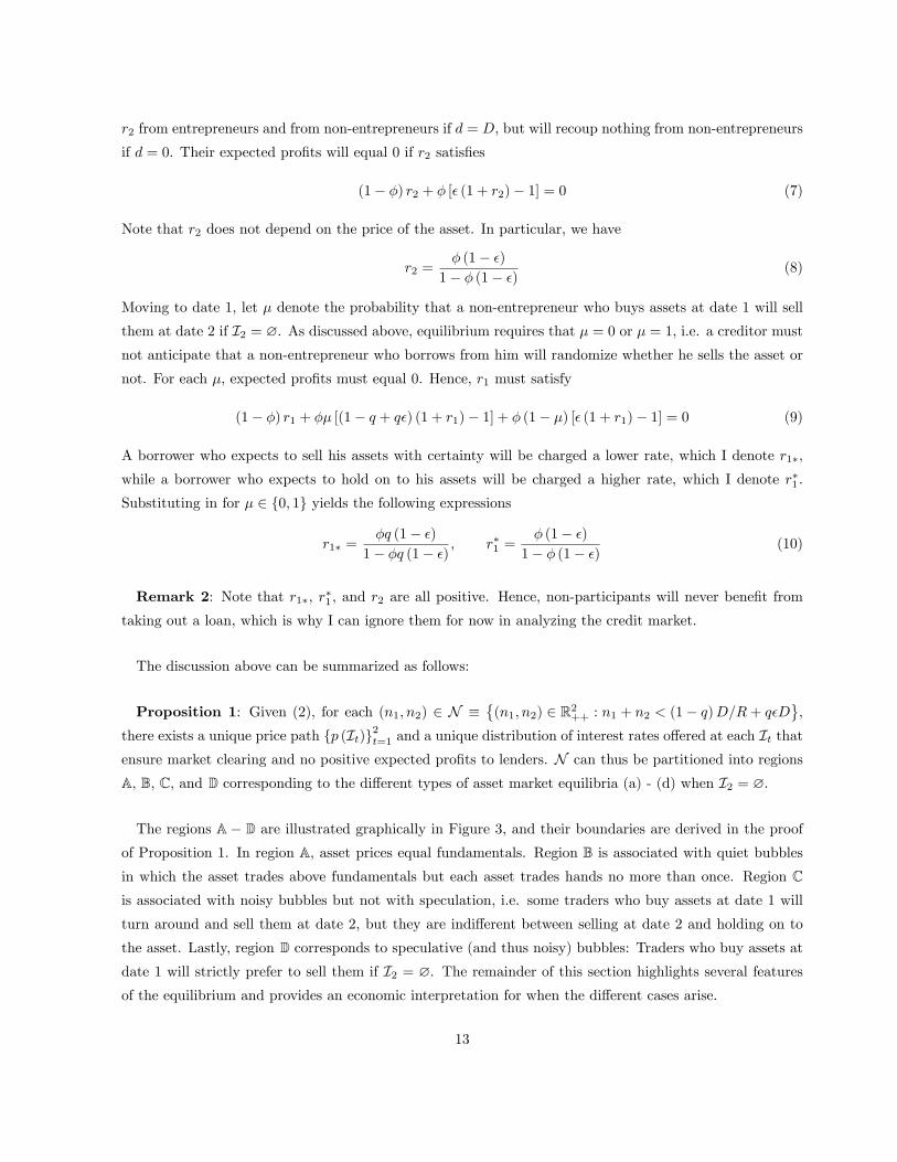
The discussion above can be summarized as follows:

Proposition 1: Given (2), for each (n1, n2) ∈ N ≡{(n1, n2) ∈ R2++ : n1 + n2 < (1− q)D/R+ qεD

},

there exists a unique price path {p (It)}2t=1 and a unique distribution of interest rates offered at each It thatensure market clearing and no positive expected profits to lenders. N can thus be partitioned into regions

A, B, C, and D corresponding to the different types of asset market equilibria (a) - (d) when I2 = ∅.

The regions A− D are illustrated graphically in Figure 3, and their boundaries are derived in the proofof Proposition 1. In region A, asset prices equal fundamentals. Region B is associated with quiet bubblesin which the asset trades above fundamentals but each asset trades hands no more than once. Region Cis associated with noisy bubbles but not with speculation, i.e. some traders who buy assets at date 1 will

turn around and sell them at date 2, but they are indifferent between selling at date 2 and holding on to

the asset. Lastly, region D corresponds to speculative (and thus noisy) bubbles: Traders who buy assets atdate 1 will strictly prefer to sell them if I2 = ∅. The remainder of this section highlights several featuresof the equilibrium and provides an economic interpretation for when the different cases arise.

13

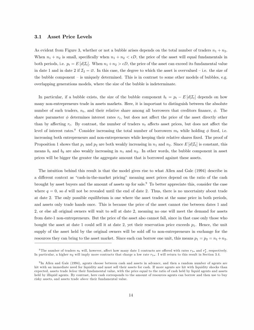
3.1 Asset Price Levels

As evident from Figure 3, whether or not a bubble arises depends on the total number of traders n1 + n2.

When n1 + n2 is small, specifically when n1 + n2 < εD, the price of the asset will equal fundamentals in

both periods, i.e. pt = E [d|It]. When n1+n2 > εD, the price of the asset can exceed its fundamental value

in date 1 and in date 2 if I2 = ∅. In this case, the degree to which the asset is overvalued —i.e. the size ofthe bubble component —is uniquely determined. This is in contrast to some other models of bubbles, e.g.

overlapping generations models, where the size of the bubble is indeterminate.

In particular, if a bubble exists, the size of the bubble component bt = pt − E [d|It] depends on howmany non-entrepreneurs trade in assets markets. Here, it is important to distinguish between the absolute

number of such traders, nt, and their relative share among all borrowers that creditors finance, φ. The

share parameter φ determines interest rates rt, but does not affect the price of the asset directly other

than by affecting rt. By contrast, the number of traders nt affects asset prices, but does not affect the

level of interest rates.8 Consider increasing the total number of borrowers mt while holding φ fixed, i.e.

increasing both entrepreneurs and non-entrepreneurs while keeping their relative shares fixed. The proof of

Proposition 1 shows that p1 and p2 are both weakly increasing in n1 and n2. Since E [d|It] is constant, thismeans b1 and b2 are also weakly increasing in n1 and n2. In other words, the bubble component in asset

prices will be bigger the greater the aggregate amount that is borrowed against these assets.

The intuition behind this result is that the model gives rise to what Allen and Gale (1994) describe in

a different context as “cash-in-the-market pricing”meaning asset prices depend on the ratio of the cash

brought by asset buyers and the amount of assets up for sale.9 To better appreciate this, consider the case

where q = 0, so d will not be revealed until the end of date 2. Thus, there is no uncertainty about trade

at date 2. The only possible equilibrium is one where the asset trades at the same price in both periods,

and assets only trade hands once. This is because the price of the asset cannot rise between dates 1 and

2, or else all original owners will wait to sell at date 2, meaning no one will meet the demand for assets

from date-1 non-entrepreneurs. But the price of the asset also cannot fall, since in that case only those who

bought the asset at date 1 could sell it at date 2, yet their reservation price exceeds p1. Hence, the unit

supply of the asset held by the original owners will be sold off to non-entrepreneurs in exchange for the

resources they can bring to the asset market. Since each can borrow one unit, this means p1 = p2 = n1+n2.

8The number of traders nt will, however, affect how many date 1 contracts are offered with rates r1∗ and r∗1 , respectively.In particular, a higher n2 will imply more contracts that charge a low rate r1∗. I will return to this result in Section 3.4.

9 In Allen and Gale (1994), agents choose between cash and assets in advance, and then a random number of agents arehit with an immediate need for liquidity and must sell their assets for cash. If more agents are hit with liquidity shocks thanexpected, assets trade below their fundamental value, with the price equal to the ratio of cash held by liquid agents and assetsheld by illiquid agents. By contrast, here cash corresponds to the amount of resources agents can borrow and then use to buyrisky assets, and assets trade above their fundamental value.

14

This intuition for why higher n1 and n2 increase the size of the bubble continues to hold with uncertainty.

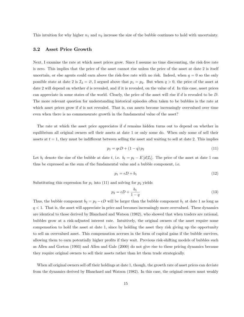
3.2 Asset Price Growth

Next, I examine the rate at which asset prices grow. Since I assume no time discounting, the risk-free rate

is zero. This implies that the price of the asset cannot rise unless the price of the asset at date 2 is itself

uncertain, or else agents could earn above the risk-free rate with no risk. Indeed, when q = 0 so the only

possible state at date 2 is I2 = ∅, I argued above that p1 = p2. But when q > 0, the price of the asset at

date 2 will depend on whether d is revealed, and if it is revealed, on the value of d. In this case, asset prices

can appreciate in some states of the world. Clearly, the price of the asset will rise if d is revealed to be D.

The more relevant question for understanding historical episodes often taken to be bubbles is the rate at

which asset prices grow if d is not revealed. That is, can assets become increasingly overvalued over time

even when there is no commensurate growth in the fundamental value of the asset?

The rate at which the asset price appreciates if d remains hidden turns out to depend on whether in

equilibrium all original owners sell their assets at date 1 or only some do. When only some of sell their

assets at t = 1, they must be indifferent between selling the asset and waiting to sell at date 2. This implies

p1 = qεD + (1− q) p2 (11)

Let bt denote the size of the bubble at date t, i.e. bt = pt − E [d|It]. The price of the asset at date 1 canthus be expressed as the sum of the fundamental value and a bubble component, i.e.

p1 = εD + b1 (12)

Substituting this expression for p1 into (11) and solving for p2 yields

p2 = εD +b11− q (13)

Thus, the bubble component b2 = p2− εD will be larger than the bubble component b1 at date 1 as long as

q < 1. That is, the asset will appreciate in price and becomes increasingly more overvalued. These dynamics

are identical to those derived by Blanchard and Watson (1982), who showed that when traders are rational,

bubbles grow at a risk-adjusted interest rate. Intuitively, the original owners of the asset require some

compensation to hold the asset at date 1, since by holding the asset they risk giving up the opportunity

to sell an overvalued asset. This compensation accrues in the form of capital gains if the bubble survives,

allowing them to earn potentially higher profits if they wait. Previous risk-shifting models of bubbles such

as Allen and Gorton (1993) and Allen and Gale (2000) do not give rise to these pricing dynamics because

they require original owners to sell their assets rather than let them trade strategically.

When all original owners sell off their holdings at date 1, though, the growth rate of asset prices can deviate

from the dynamics derived by Blanchard and Watson (1982). In this case, the original owners must weakly

15

prefer to sell the asset for price p1 at date 1 than to hold it and sell at date 2, and so p1 ≥ qεD+(1− q) p2.Thus, (1− q)−1 represents an upper bound on the rate at which the bubble can grow. But there is also alower bound on the rate at which the bubble can grow. In particular, if all original owners sell their assets

at date 1, non-entrepreneurs who show up at date 2 will have to buy assets from non-entrepreneurs who

arrived at date 1. The latter will only agree to sell if the price is at least equal to their reservation price,

εD + (1− ε) (1 + r1∗) p1. Hence, the price of the asset p2 must satisfy

εD + (1− ε) p1 (1 + r1∗) ≤ p2 ≤ εD +b11− q (14)

We know from Lemma 1 that p1 (1 + r1∗) < D, and so the lower bound on p2 implies that p2/p1 ≥ (1 + r1∗),i.e. the price of the asset must grow faster than the rate at which non-entrepreneurs must pay to borrow

resources.10 This is because non-entrepreneurs who sell the asset at date 1 must not only earn enough to

pay their creditors, but must be compensated for the option value of default they give up and which they

could have exercised if they held on to their assets. Intuitively, price appreciation in this case is driven by

the fact that an increase in price allows for trade. In particular, if the price of the asset rises, agents who

buy the asset borrow more against each asset than those from whom they buy the assets. As a result, the

option to default is more valuable for new buyers than it is to its existing owners, meaning they will value

the asset more than the original cohort of buyers. The implied rate of price appreciation may be slower

than the growth rate due to the considerations first pointed out by Blanchard and Watson (1982). Since

this lower rate of price appreciation occurs when the original owners sell all of their asset holdings at date

1, asset price appreciation will generally be lower when trade volume in the bubble asset is high early on.

In sum, the rate at which the bubble component grows depends on when traders show up and is bounded

by (1− q)−1, a bound which is increasing in the probability of the bubble bursting. This insight suggests whythe phenomena that distinguish historical episodes suspected to be bubbles, e.g. rapid price appreciation,

might be rare. When rapid appreciation is possible, i.e. when q is large, appreciation is also less likely

to materialize since the bubble is likely to burst. However, the fact that we observe rapid asset price

appreciation only infrequently does not imply that bubbles — instances in which assets are overvalued —

are also inherently rare. In particular, quiet bubbles associated with low values of q can be quite common,

although they are also harder to identify empirically since this requires estimating fundamentals.

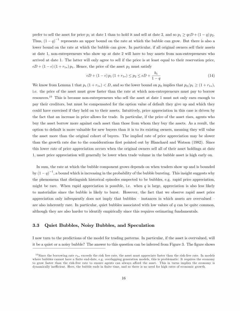
3.3 Quiet Bubbles, Noisy Bubbles, and Speculation

I now turn to the predictions of the model for trading patterns. In particular, if the asset is overvalued, will

it be a quiet or a noisy bubble? The answer to this question can be inferred from Figure 3. The figure shows

10Since the borrowing rate r1∗ exceeds the risk free rate, the asset must appreciate faster than the risk-free rate. In modelswhere bubbles cannot have a finite end-date, e.g. overlapping generation models, this is problematic: It requires the economyto grow faster than the risk-free rate to ensure agents can always afford the asset. This in turns implies the economy isdynamically ineffi cient. Here, the bubble ends in finite time, and so there is no need for high rates of economic growth.

16

the nature of the asset market equilibrium at date 2 for different values of n1 and n2. Recall that region

B corresponds to quiet bubbles where assets trade hands only once, while regions C and D correspond tonoisy bubbles where at least some of the agents who buy assets at date 1 will sell them at date 2. Figure

3 is drawn as if all four types of equilibria are possible. However, this will not be true in general. In

particular, whether equilibria corresponding to regions C and D are possible depends on the location of theouter boundary for region B relative to the outer boundary of the set N . If the outer boundary for region B—whose location depends on the parameters q, ε, and φ —is suffi ciently far away from the origin, then the

only type of equilibrium bubbles that can arise for (n1, n2) ∈ N are quiet bubbles. Whether speculation

and noisy bubbles can arise depends on these parameters.

The formal analysis of how these parameters affect the types of equilibria is contained in the Appendix.

Here, I only review the results. Consider first q, which I argued in Section 3.2 governs the rate at which

the bubble can grow. As q → 0, region B expands outwards to cover all pairs (n1, n2) ∈ N for which

n1 + n2 > εD. In other words, for small q, only quiet bubbles are possible. Intuitively, the smaller the

risk of the bubble collapsing, the less the bubble can grow over time without inducing agents to hold on to

the asset. But if asset prices do not grow much over time, traders who borrow to buy the asset will not

earn enough when they sell the asset to cover their interest obligation and the option value to default they

give up by selling the asset. Hence, noisy bubbles will not arise for low values of q. Can they arise for high

values? As q → 1, region B shrinks towards the origin, meaning fewer values of (n1, n2) will be associatedwith quiet bubbles. However, the set N also shrinks. In the Appendix, I show that if R is close to its upper

bound of 1/ε, noisy bubbles will exist for some (n1, n2) ∈ N when q is close to 1. When R is close to its

lower bound in (2), noisy bubbles still exist for some (n1, n2) ∈ N when q is close to 1 and either ε or φ are

large. Since q governs the rate at which asset prices can appreciate, it follows that noisy bubbles are more

likely to arise when price appreciation is high. As in Section 3.2, it also follows that speculative trading will

be rarely observed, since when it can take place the bubble is likely to burst before speculators can sell.

Turning to ε, in the limit as ε→ 1, any (n1, n2) ∈ N for which n1+n2 > εD must fall in region B. Thus,when ε is large, if there is a bubble it must be a quiet bubble. In the opposite direction, as ε→ 0, then as

long as q < 1, in the limit all (n1, n2) ∈ N lie in either region C or D. That is, when ε is small, bubblesmust arise and are inherently noisy.11 To understand this result, note that for small values of ε, holding

on to the asset is likely to be unprofitable, since d is likely to assume its low realization. Thus, a high ε

will encourage those who buy the asset early to turn around and sell it rather than hold on to it. This

suggests penny stocks, i.e. stocks that trade at low prices but have a skewed return distribution, should

be particularly vulnerable to speculative bubbles. Interestingly, Eraker and Ready (2013) find that such

11 Interestingly, Hong and Sraer (2011) also find that noisy bubbles are more likely for assets with a high upside potential,but for different reasons. In particular, a high upside in their model allows for more potential for disagreement as to the valueof the asset, which encourages trade. This feature is absent from my setting.

17

stocks seem to be overvalued, since they tend to have a negative expected return that cannot be explained

by asset characteristics. As for φ, region B becomes larger as φ rises, i.e. higher values for φ are more likelyto be associated with quiet bubbles. Intuitively, a higher φ increases the cost of borrowing, which raises the

reservation price of agents who borrowed to buy the asset. High values of φ thus discourage turnover.

While q, ε, and φ determine whether bubbles can be noisy, it is clear from Figure 3 that when noisy

bubbles are possible, they occur only when either n1 or n2 are large. Intuitively, noisy bubbles require that

either a lot of traders buy at date 1 who can later sell, or else a large number arrive and wish to buy assets

at date 2. Recall from Subsection 3.1 that other things equal, higher values of n1 and n2 imply the asset

will be more overvalued. This implies that noisy bubbles will tend to be associated with assets that are

more overvalued, while assets that are only slightly overvalued will be associated with quiet bubbles. What

is not evident from Figure 3 is that too much overvaluation discourages noisy bubbles. In particular, if

n1 + n2 > qεD + (1− ε)D/R, we can no longer use (3) to ensure that all non-entrepreneurs will buy theasset. Although I omit the formal analysis of this case, with a large number of traders the expected profits

from buying the asset will turn to zero. This will reduce the volume of trade associated with the asset.

Although either n1 or n2 must be large for bubbles to turn noisy, the role of n1 and n2 in contributing to

noisy bubbles is not symmetric. On the one hand, holding the total number of non-entrepreneurs n1 + n2

fixed, a noisy bubble is more likely to arise if most traders arrive early rather than late, i.e. when n1 is large

rather than n2. Intuitively, if a lot of traders show up at date 1, they will have to be those who sell the asset

at date 2 if there is additional demand. But if few traders show up at date 1, additional demand at date

2 might still be potentially met by original owners. At the same time, the features most associated with

historical episodes suspected to be bubbles arise when n2 is large rather than n1. First, recall from Section

3.2 that asset price growth is likely to be higher when n1 is small. In addition, Figure 3 reveals that region

D where speculative bubbles arise requires that n2 be large relative to n1. Thus, scenarios with rapid assetprice growth and traders who are keen to both buy and sell assets are more likely to be associated with a

rising trade volume rather than a falling one.

3.4 Borrowing Rates in Credit Markets

Finally, many of the historical episodes suspected to be bubbles are associated with low interest rates charged

to those who borrow against supposedly bubble assets. This may seem at odds with the risk-shifting view of

bubbles: Since risk-shifting requires creditors to charge higher spreads to cover losses on speculators, spreads

should presumably be higher with bubbles than when bubbles are absent. However, my model implies that

noisy bubbles can be associated with lower borrowing rates than quiet bubbles. Whether historical episodes

should be associated with high or low borrowing spreads depends on whether the tranquil times against

which these episodes are judged are periods in which asset prices reflect fundamentals or in which the assets

18

exhibit quiet bubbles. In principle, as noted by Diba and Grossman (1987), assets that can potentially

exhibit bubbles in the future must contain a bubble component in the present, even if it is arbitrarily small.

Since we argued in Section 3.3 that small overvaluation is likely to be associated with quiet bubbles, it

seems reasonable to view tranquil times as periods in which the asset is slightly overvalued.

To see that noisy bubbles can be associated with lower borrowing spreads than quiet bubbles, consider

the effect of increasing the absolute number of non-entrepreneurs n2 who arrive at date 2 while holding

their share among total borrowers φ fixed. Graphically, this implies moving up along Figure 3. The higher

is n2, the larger the fraction of date 1 buyers who will have to sell their assets. Thus, as long as we are in

an equilibrium of type (c), more borrowers will be offered a low rate r1∗ rather than a high rate r∗1 , until

eventually we move into an equilibrium of type (d) in which all the agents who buy at date 1 will sell at

date 2 if the payoff on the asset remains uncertain. The intuition for this is due to dynamic risk-shifting:

When traders turn around and sell the overvalued assets they buy, their lenders will anticipate that part

of the risk from lending against an overvalued asset will be borne by future lenders. This allows them to

charge lower rates to their borrowers. However, since noisy bubbles are more likely at high values of q, the

lower rate r1∗ may not be substantially lower than r∗1 since much of the risk is still associated with early

periods. In the next section, where I let creditors choose from a larger set on contracts, I discuss another

reason for why speculative bubbles may be associated with low spreads.

3.5 Summary

The preceding analysis shows that risk-shifting models of bubbles in which assets can trade above their

fundamental value may give rise to patterns consistent with historical episodes taken to be bubbles, e.g. rapid

price appreciation, speculative trading, and low spreads charged to those who borrow against assets used

for speculative trading. However, an overvalued asset will not always exhibit these patterns. Assets that are

only slightly overvalued will tend to trade infrequently and can exhibit low rates of price appreciation. More

overvalued assets, especially those with a high trade volume and against which a large amount is borrowed,

are those that are prone to become speculative bubbles. But since rapid appreciation and speculation can

only be high when bubbles are likely to burst early, such patterns should be observed relatively infrequently.

4 Endogenous Contracts

Up to now, I allowed creditors to offer only fixed-size, full-recourse, simple debt contracts. In this section,

I allow lenders to choose from a broader set of contracts. This serves two purposes. First, it offers a

robustness exercise: Can speculative bubbles still emerge when lenders can choose from a broader set of

contracts? Second, it reveals what types of contracts will emerge when speculative bubbles arise. To

19

preview my results, I find that endogenizing contracts makes it harder but not impossible for bubbles to

occur: Although lenders would like to avoid funding agents who plan to buy overvalued assets, they will not

always be able to avoid doing so. When lenders cannot avoid taking on non-entrepreneurs, they will design

contracts to minimize losses on non-entrepreneurs, and the purchase of overvalued assets will be financed

using certain types of contracts. In particular, my model gives rise to Spence-Miyazaki-Wilson contracts,

along the lines of Spence (1977), Miyazaki (1977), and Wilson (1977), whereby creditors earn profits on

entrepreneurs that cross-subsidize the minimal losses possible on non-entrepreneurs.

Analyzing contract choice requires being more explicit about what agents know and can condition their

contacts on. In line with my focus on debt contracts, I consider a costly state verification model as in

Townsend (1979) and Gale and Hellwig (1985) that gives rise to debt-like contracts. That is, creditors

cannot immediately observe what assets borrowers purchased. However, at the end of date 2, creditors can

learn what assets the borrower purchased as well as their cash holdings by paying a cost. The auditing

cost is assumed to be a fraction λ < 1 of the borrower’s cash holdings, meaning it is less costly to audit

agents with fewer resources to hide. Assuming a purely proportional cost is analytically convenient, since

it implies an agent with no cash can be audited at no cost. Adding a fixed cost of verification would not

fundamentally change my results as long as the fixed cost component was small, but it would raise the issue

of stochastic auditing as a way to minimize auditing costs. I wish to avoid randomization, not just because

it is rarely employed in practice but because it raises some technical issues that I discuss below. In what

follows, I assume λ is close to 1. As I discuss below, a suffi ciently high value for λ will deter lenders from

auditing borrowers who claim to be entrepreneurs unless they fail to pay the amount required of them.

Appealing to the revelation principle, we can replicate any contract with a direct mechanism in which

borrowers report their private information, and these reports trigger transfers as well as an audit strategy.

Transfers can only depend on the borrower’s actual private information if the lender audits the borrower.

Contracts can of course still depend on publicly observable information, e.g. payments can depend on I2 ord even if creditors do not observe whether a given borrower bought risky assets. However, this conditioning

is possible only because I’ve assumed one type of risky asset. With more than one type of risk asset, such

conditioning might not be possible. In particular, suppose that we allowed for a continuum of ex-ante

identical risky assets, all of which pay a single dividend d distributed according to (1). However, ex-post,

only a fraction ε pay out d = D, and for a fraction q of each type of asset the value of d is revealed before

date 2. Non-entrepreneurs who secure funds would prefer to concentrate in one asset rather than diversify,

and each period non-entrepreneurs would spread out uniformly across all assets whose dividend remains

uncertain. As long as we adjust the number of traders in period 2 to account for the fact that fewer assets

will trade at date 2 than at date 1, we can reinterpret the model in the previous section with only one type

of asset as one with different assets but no aggregate uncertainty and thus nothing for lenders to condition

20

on.12 Motivated by this interpretation, I consider contracts that do not condition on asset market variables.

This also leads to a contract that more closely resembles a standard debt contract.13

Formally, a contract amounts to a sequence of announcements by borrowers at the various stages where

they have private information, and a sequence of transfers and actions triggered by these announcements. I

use θj denote the reports at stage j = 1, 2, 3, ... and xj(θj) as the transfer from the borrower following each

report. Figure 4 summarizes the contract for agents who arrive at date 1 as a flow chart. The contract for

agents who arrive at date 2 can be constructed similarly.

A contract begins with an agent reporting upon his arrival whether he is an entrepreneur (denoted θ1 = e)

or not (θ1 = n). While I could allow non-entrepreneurs and non-participants to distinguish themselves, this

turns out to be unnecessary. The contract then stipulates a transfer x1(θ1) from the creditor to the borrower.

Since agents own no resources, x1(θ1) ≥ 0.

The next stage at which the agent has private information is after he chooses what to do with the funds

he received. Assumptions (2) and (3) ensure agents will not be indifferent between actions, and will allocate

all of the funds they receive to a single use. This simplifies what agents can report. An agent who reported

he was an entrepreneur can only truthfully report that he either initiated entrepreneurial activity (θ2 = e)

or did nothing (θ2 = ∅), and so without loss of generality I restrict agents to these two reports. An agentwho reported he was not an entrepreneur can only truthfully report that he bought assets (θ2 = b) or did

nothing (θ2 = ∅), so I restrict him to these two reports. Let x2(θ1, θ2) denote the transfer from the lender

to the borrower following this report. If the agent reports that he used his funds, i.e. θ2 ∈ {e, b}, he wouldhave no resources to transfer if he were truthful, so x2(θ1, θ2) ≥ 0. If the agent reports he did nothing, theconstraint is x1(θ1) + x2(θ1, θ2) ≥ 0, i.e. he cannot transfer more resources than he originally received.

For agents who arrive at date 1, the next stage at which they may receive private information is at the

beginning of date 2, after the asset market clears but before d and R are paid out. At this point, an agent

who reported buying assets, i.e. θ2 = b, must report whether he sold his assets before d was revealed

(θ3 = p2), sold them after learning d is high (θ3 = D), sold them after learning d is low (θ3 = 0), or held

on to them (θ3 = h). An agent who reports θ2 ∈ {e,∅} would have nothing to report at this stage if hewere truthful. For completeness, I let them report θ3 = ∅. Let x3(θ1, θ2, θ3) denote the net transfer fromthe lender to the borrower after report θ3 is submitted.

12 In particular, if we want the mass of traders at date 2 to equal n2, the number of traders who arrive must equal n2/ (1− q).

13Allowing contracts to condition on the asset market would not change my qualititative results. In particular, it wouldlead creditors to charge high payments in states where non-entrepreneurs earn profits, e.g. if d = D, and low (even negative)payments in other states. However, the most a contract can demand from entrepreneurs in any state is R, and assumption(3) implies the return to buying the risk asset and holding it to maturity exceeds R. Hence, non-entreperneurs would want totrade with creditors if contracts were contingent on asset market data.

21

At the end of date 2, an agent must issue a final report on his earnings. I denote this report y. If the

initial transfer x1(θ1) > 0, it will be convenient to let y denote earnings divided by x1(θ1). If x1(θ1) = 0,

the agent cannot do anything anyway, so I can restrict him to reporting y = 0. When x1(θ1) > 0, five

reports are possible for y: R − 1, if the agent chose to produce; p2/p1 − 1, if the agent bought and soldassets before learning d; D/p1 − 1, if d = D and the agent did not sell the assets before d was revealed;

−1, if d = 0 and the agent did not sell the asset before d was revealed; and 0, if the agent did nothing. Ilet the agent report any of these y regardless of previous reports. In particular, I need to let an agent who

bought assets but pretended to engage in entrepreneurial activity come clean if d = 0. After these reports,

the lender can choose whether to audit the agent. This means that the contract must specify an auditing

rule σy(θ1, θ2, θ3, y) equal to 1 if the agent is audited and 0 otherwise. I do not allow for stochastic audits

where 0 < σy < 1. This restriction prevents a lender from offering a contract with a slightly higher audit

probability and a slightly lower interest rate that would attract entrepreneurs who have no reason to fear

auditing. Allowing lenders to offer such contracts would imply no equilibrium exists, for the reason pointed

out in Rothschild and Stiglitz (1976): Any potential equilibrium would be vulnerable to cherry-picking of

good types. Restricting contracts to deterministic audits is one way to address this non-existence problem.

Other approaches would allow for stochastic auditing, but are considerably more involved.14

Finally, the contract stipulates a transfer xy(θ1, θ2, θ3, y) from the lender to the borrower if there is no

audit, and a transfer xy(θ1, θ2, θ3, y, y) if there is an audit, where y denotes actual earnings.

Now that I’ve described contracts, I can proceed to characterize equilibrium contracts. Since the lender

chooses contracts optimally, I begin with some observations about optimal contracts. First, suppose a

borrower announces he has no cash at the end of date 2, i.e.

x1(θ1) + x2(θ1, θ2) + x3(θ1, θ2, θ3) + yx1(θ1) = 0 (15)

If this report is truthful, the agent will not be able to make any transfers, and so xy(θ1, θ2, θ3, y) ≥ 0. Assuch, it will be optimal for the lender to audit the borrower and grab all of his resources if he is untruthful.

The reason is that if the agent is telling the truth then the audit is costless, while if he is not telling the

truth the agent can be punished. Since λ < 1, auditing and punishing an agent is never costly for the

lender. At the same time, punishing false reports relaxes incentive constraints, so the lender should do it.

A second observation is that a lender can use transfers to limit the misreports agents can make. In

particular, if x1(θ1) > 0, the lender can confirm a report that the agent did nothing with his funds, i.e.

θ2 = ∅, by asking the agent to transfer back his resources, i.e. x2(θ1, θ2) = −x1(θ1). This would only

14Wilson (1977), Miyazaki (1977), and Spence (1977) suggested dealing with this non-existence by redefining equilibrium sothat an equilibrium contract cannot be improved upon only by contracts that remain profitable when unprofitable contractsare withdrawn. Mimra and Wambach (2011) and Netzer and Scheuer (2013) provide game-theoretic foundations for this ideaby allowing lenders withdraw contracts (possibly at a small cost) after observing the contracts offered by others.

22

be feasible if θ2 = ∅. Subsequent transfers can then be used to achieve any desired terminal payoff forthis type. Likewise, the lender can confirm whether an agent who bought assets at date 1 sold them at

date 2 for a positive price, i.e. θ3 ∈ {p2, D}, by asking the agent to transfer more than x1(θ1) after thisannouncement, i.e. x2(θ1, θ2) < x1(θ1). Again, this would only be feasible if the agent in fact bought and

sold assets. Lastly, the lender can verify whether the agent earned D per asset by requiring an agent who

reports y = D/p1 − 1 to transfer D/p1. The upper bound on R in (2), together with (3), puts a limit on

the price p2, implying that D/p2 > R. Thus, a non-entrepreneur who buys assets has enough funds to pass

himself off as an entrepreneur, but not vice-versa. Note that confirming an agent earned y = D/p1− 1 mayrequire an additional transfer after xy(θ1, θ2, θ3, y) to achieve a given payoff to the borrower, i.e. the agent

and lender must transfer resources back and forth. These transfers greatly limit the type of misreports by

agents and thus reduce the number of incentive constraints the contract is subject to.

The last observation is that it will be optimal for the lender to audit the agent and seize all of his cash

if the agent is ever inconsistent in his reports, e.g. announcing that he bought assets but then reporting

y = R−1. This implies that in equilibrium, an agent who reports he chose to produce, i.e. θ2 = e, will have

to pay some amount if he reports his income is R− 1, and will be audited and left with no cash otherwise.Likewise, an agent who reports he bought assets, i.e. θ2 = b, will have to pay some amount that may depend

on what he says he did with the assets he bought, and will be audited and left with no cash otherwise.

We can use the observations above to determine when the equilibrium contract will call for an audit.

First, without loss of generality, an agent who announces y = −1 without contradicting past reports will beaudited. This is because we can always take the equilibrium contract and construct an equivalent contract

with x2(θ1, θ2) = x3(θ1, θ2, θ3) = 0 for reports consistent with a report of y = −1, ensuring the agent willhave no cash at the end of date 2 if the true y = −1. This allows the lender to audit at no cost if the agentis truthful while discouraging misreports. If we set xy(·) to ensure the same terminal payoff to a truthfulagent as in the original contract, this contract will do at least as well as the original equilibrium contract.

Next, suppose the agent reports y = 0 or y = D/p1−1. Since the lender can directly confirm these reportsusing transfers, neither report will be audited in equilibrium. The lender cannot fully verify y = p2/p1 − 1,since an agent who sells his assets early at price D can pass himself as this type. Since lenders prefer non-

entrepreneurs sell their assets if d is not revealed, they may want to audit such reports to reward agents.

For now, I take no stand on whether this report will be audited, although I argue below that it will not.

Finally, suppose the agent reports y = R − 1. As anticipated above, it will be optimal not to audit theborrower following this report if λ is close to 1. For suppose the optimal contract did audit agents making

this report. As λ→ 1, the rate that must be charged to entrepreneurs to ensure non-negative profits must

tend to R, since auditing costs on these agents are equal to λR while the expected profit from lending to

non-entrepreneurs is negative. At the same time, the first inequality in (2) implies there exists a rate strictly

23

below R such that charging this rate to all borrowers and collecting it in full from entrepreneurs and with

probability ε from non-entrepreneurs will yield positive profits. Since the latter is a lower bound on the

profits of the lender, it follows that as λ ↑ 1, not auditing a report of y = R− 1 will be optimal.

It follows that equilibrium contracts are essentially variable-size debt contracts with a repayment schedule:

An agent who arrives at date 1 and reports θ1 ∈ {e, n} receives xθ11 resources together with a particular

repayment schedule. An agent who reports θ1 = e will be asked to pay back (1 + re1)xe1 at the end of date

2 or else be audited. An agent who reports θ1 = n will be asked to pay back an amount that depends on

when he pays. If he waits until the end of period 2, meaning he reported holding on to his assets (θ3 = h),

he will have to pay xn1 (1 + rn,late1 ) and will be audited otherwise. If he pays at the beginning of date 2,

meaning he sold assets for a positive price, he would owe xn1 (1+rn,D1 ) if he sold at price D and a potentially

different amount xn1 (1+rn,p21 ) if he sold at price p2. If he pays earlier still at date 1, meaning he did nothing

(θ2 = ∅), he would owe xn1 (1 + rn,∅1 ). That is, the borrower either receives xe1 with a requirement to repay

at rate re1 at the end of date 2, or he receives xn1 with a rate schedule

{rn,∅1 , rn,D1 , rn,p21 , rn,late1

}. This

description abstracts from the back-and-forth transfers to verify the borrower’s reports that are needed to

sustain the contract, but it correctly capture the terminal payoffs to the lender.

By a similar argument, an agent who arrives at date 2 receives a variable-size debt contract depending

on his report θ1 ∈ {e, n} that specifies an initial transfer xθ12 and an amount he must repay at the end of

period 2, but which might charge a different rate if he shows he did nothing with the funds he received.

Given the optimal audit rules I derived above, agents who report θ1 = n will at some point be either

audited or forced to make a transfer that reveals their identity. As such, we need not worry about whether

entrepreneurs will try to report θ1 = n. Instead, the relevant incentive constraints are that non-entrepreneurs

not try to pass themselves as entrepreneurs or misreport when they sold assets or for how much. Alas for

lenders, these incentive constraints have real bite, since non-entrepreneurs can secure themselves positive

expected profits from pretending to be entrepreneurs. In particular, they can buy risky assets and hold them

to the end of date 2, then pay back no more than R < D/p if d = D, all without being audited. Creditors

who want to to fund entrepreneurs thus have no choice but to also take on non-entrepreneurs and offer them

rents. However, it does not follow from this that once creditors finance entrepreneurs, non-entrepreneurs

must end up buying risky assets. Rather, creditors can provide rents to non-entrepreneurs by paying them

off rather than lending to them. Formally, they can offer rn,∅1 < 0, essentially paying non-entrepreneurs not

to buy assets. The next proposition establishes that if all agents without a production opportunity can buy

risky assets —meaning all can participate in the asset market —it would indeed be optimal for creditors to

bribe non-entrepreneurs not to buy the asset, and a bubble would not emerge.

Proposition 2: If there are no non-participants, allowing lenders to choose contracts optimally implies

that the equilibrium price of the asset must be p1 = p2 = εD, i.e. bubbles will not emerge.

24

Intuitively, letting a non-entrepreneur buy an overvalued asset is a costly way for the creditor to provide

him with rents: When the asset is overvalued, the creditor ends up paying some resources to whoever the

non-entrepreneur buys the asset from beyond the rents he provides the non-entrepreneur. Thus, where there

is a bubble, it is more effi cient to pay agents directly than to reward them by having them buy assets.

Paying agents not to buy risky assets may not work well in practice, however. The reason is that it

may draw in people who have no intention to speculate. Here is where non-participants finally play a role.

While they do nothing in equilibrium, their presence precludes creditors from paying non-entrepreneurs not

to speculate. As long as there are enough non-participants, the cost of having to pay them together with

non-entrepreneurs will be enough to make contracts with rn,∅1 < 0 too costly, and creditors who need to

deliver rents to non-entrepreneurs will choose to do so by letting the latter purchase risky assets.

Formally, if there is a large enough group of non-participants, any contract must satisfy the property

that if the cumulative transfers from the creditor to the borrower are positive —i.e. if the lender ends up

giving any gift to the borrower — it must be that the borrower has zero cash holdings at the end of date

2. Otherwise, agents with no intention to buy risky assets will also accept the contract. Since an agent

with zero cash holdings will be audited in equilibrium, this restriction can be formalized as follows. First,

if there is no audit, net transfers from the lender to the borrower must be non-positive:

x1(θ1) + x2(θ1, θ2) + x3(θ1, θ2, θ3) + xy(θ1, θ2, θ3, y) ≤ 0 (16)

Second, if there is a positive transfer of resources from the creditor to the agent with auditing, then the

terminal cash holdings of the agent must be 0, i.e.

x1(θ1) + x2(θ1, θ2) + x3(θ1, θ2, θ3) + xy(θ1, θ2, θ3, y) > 0 (17)

implies

x1(θ1) + x2(θ1, θ2) + x3(θ1, θ2, θ3) + xy(θ1, θ2, θ3, y, y) + y · x1(θ1) = 0 (18)

Under these conditions, non-participants will never find it profitable to borrow. We can therefore ignore

them for the remainder of our discussion: Creditors will never have to engage them, and their only role

comes from imposing the additional constraints (17) and (18) on contracts.

Since the first inequality in (2) ensures it will be profitable to finance entrepreneurs, we can conclude that

xe1 = xe2 = 1, i.e. entrepreneurs receive the maximum amount of funding they can employ productively.

Otherwise, a lender could simply scale xet and xnt up proportionally but charge entrepreneurs slightly more

than under the original contract, a small enough increase that they would still prefer to borrow a larger

amount at a slightly higher rate. Since entrepreneurs cannot pass themselves off as non-entrepreneurs, they

will choose the contract designed for them. Non-entrepreneurs will prefer the contract offered to them

given that under the original equilibrium they preferred the contract offered them when entrepreneurs were

25

charged a lower rate. Since scaling up both loans and leaving interest rates fixed would leave profits at zero,

charging entrepreneurs higher rates ensures positive profits. Hence, xet < 1 cannot be an equilibrium.

The only remaining terms of the contracts offered to entrepreneurs are the rates re1 and re2. Since lenders

earn zero expected profits in equilibrium, the amount collected from entrepreneurs must equal the expected

losses on non-entrepreneurs. This, in turn, depends on the terms offered to non-entrepreneurs. To solve for

these, I begin with a preliminary result. Let Vt(θ1, θ1) denote the expected utility to an agent of type θ1 who

announces his type as θ1 and then behaves optimally. The next lemma establishes that in equilibrium, a

non-entrepreneur will be indifferent about what type he announces:

Lemma 2: In equilibrium, Vt (n, n) = Vt (n, e)

Lemma 2 implies that the equilibrium contract offered to non-entrepreneurs solves the problem of max-

imizing the expected revenue from non-entrepreneurs while leaving the non-entrepreneur with the same

utility as if he reported θ1 = e. For suppose the equilibrium contract did not solve this problem, i.e. there

exists a contract x′ that offers identical terms to entrepreneurs and leaves non-entrepreneurs with the same

utility Vt (n, e) but collects more revenue from them. A lender could then offer a contract x′′ equivalent to x′

but which charges non-entrepreneurs slightly less so that their utility under x′′ is still higher than Vt (n, e).

This allows the lender to also charge entrepreneurs slightly less than under the original equilibrium contract

without inducing non-entrepreneurs to report θ1 = e. Since the original contract earned zero profits, x′

would generate positive profits if it attracted both types since it collects more from non-entrepreneurs but

the same amount from entrepreneurs. Since the profits from x′′ can be made arbitrarily close to the profits

from x′ when it attracts both types, it follows that the original contract could not have been an equilibrium.

Essentially, the creditor would like to grab as much resources from non-entrepreneurs to make his contract

as attractive as possible to entrepreneurs.

Applying this insight, we can solve for the equilibrium contracts offered to agents who show up at date 2.

In particular, the terms offered to non-entrepreneurs who arrive at this date can be summarized by a loan

size xn2 and a repayment rate rn2 that satisfy

maxxn2 ,r

n2

xn2 [ε (1 + rn2 )− 1] (19)

subject to

i. ε

(D

p2− (1 + rn2 )

)xn2 = ε

(D

p2− (1 + re2)

)ii. rn2 ≥ 0

Constraint (i) corresponds to the requirement that V2 (n, n) = V2 (n, e). Constraint (ii) follows from the

requirement that rates cannot be negative given (17) and (18). Solving (19) yields

26

Proposition 3: In an equilibrium where p2 > εD, non-entrepreneurs will be offered a contract in which

xn2 =D−(1+re2)p2

D−p2 < 1 and rn2 = 0, while entrepreneurs will be offered a contract where xe2 = 1 and r

e2 solves

(1− φ) re2 + xn2φ (εre2 − (1− ε)) = 0.

To understand this result, observe that creditors always want to lend less to non-entrepreneurs, but they

need to charge a lower rate on such loans to ensure non-entrepreneurs choose these contracts which may

not make them so profitable. When p2 > εD, it turns out that lenders do not need to lower rates too much

to attract non-entrepreneurs to smaller loans. In particular, lenders will find it optimal to lower interest

rates and offer non-entrepreneurs smaller loans, up to the point where they hit the constraint that interest

rates must be nonnegative. This reveals a distinct reason for why speculative bubbles might be associated

with low spreads between the borrowing rate and the risk-free rate: In order to steer agents who intend to

buy risky assets towards contracts that incur smaller losses for lenders, these loans must carry low rates.

Remark 5: The fact that lenders do not need to worry about entrepreneurs pretending to be non-

entrepreneurs plays an important role behind Proposition 3. If entrepreneurs could pass themselves off as

non-entrepreneurs, e.g. if they could engage in hidden borrowing or if we precluded back-and-forth transfers

that would allow non-entrepreneurs to prove their types, we would need to add a constraint to (19) to insure

the entrepreneur does not prefer to take the smaller loan at a low rate, i.e.

R− (1 + re2) ≥ (R− (1 + rn2 ))xn2

Comparing this constraint with (i) reveals that the nature of the equilibrium contract depends on how

D/p2 compares to R. When D/p2 > R, the fact that non-entrepreneurs are just indifferent between a

higher rate on a large loan and a zero rate on a small loan implies entrepreneurs would prefer the smaller

loan. In that case, in equilibrium both types will be offered the same contract, i.e. xn2 = xe2 = 1 and

re2 = rn2 =(1− ε)φ

1− (1− ε)φ . That is, if lenders are precluded from using transfers to restrict what borrowers

can report, the equilibrium contract terms may be the same for both types. �

Finally, consider contracts offered to agents who arrive in period 1. A few observations allow me to

simplify the characterization of these contracts. As in the previous section, in equilibrium lenders must

believe the non-entrepreneurs they lend to will either hold or sell their assets at date 2 with certainty if d

is not revealed. For lenders who expect a borrower to hold on to his assets, the equilibrium contract can be

described as a simple long-term debt contract {xn1 , rn,late1 } in which the agent receives xn1 upon arrival and

is asked to repay xn1(1 + rn,late1

)at the end of date 2 or else be audited. To see this, denote the original

loan amount by xn1 . Since rates must be nonnegative, agents will prefer buying assets to doing nothing,

so we can ignore the rate for repayment at date 1. Denote the remaining rates by {rn,D1 , rn,p21 , rn,late1 }.Construct a new contract {xn1 , r

n,late1 } where xn1 = xn1 and r

n,late1 = qrn,D1 + (1− q) rn,late1 . If the borrower

27

holds on to his assets, he will only repay if d = D. Under the original contract, he would have expected to

pay qrn,D1 + (1− q) rn,late1 with probability ε. The same is true for the new contract. If the agent prefers to

sell his assets under the new contract if d is not revealed, the original contract could not have been optimal,

since the new contract recoups the same expected amount but with a larger probability. Since all agents

are indifferent between the new contract and the original equilibrium contract, and the trading strategy of

non-entrepreneurs is unchanged, the contract {xn1 , rn,late1 } is equivalent to the original equilibrium contract.

Next, consider a borrower who intends to sell his assets. Here the equilibrium contract can be represented

using a simple short-term debt contract {xn1 , rn,early1 } in which the agent receives xn1 upon arrival and is

asked to repay xn1(1 + rn,early1

)at the beginning of date 2 or else be audited and be stripped of all of his

cash holdings. To see this, denote the terms of the equilibrium contract by xn1 and {rn,D1 , rn,p21 , rn,late1 }.

Construct a new contract {xn1 , rn,early1 } where xn1 = xn1 and r

n,early1 = 1−q

qε+(1−q) rn,p21 + qε

qε+(1−q) rn,late1 . If the

borrower intends to sell his assets, this contract would ensure the same expected repayment. But a borrower

who accepts a short-term contract would necessarily sell the asset early at date 2. Hence, the short-term

contract {xn1 , rn,short1 } is equivalent to the original contract, since all agents are indifferent between this and

the original equilibrium contract and it has no effect on the trading strategy of non-entrepreneurs.

We can therefore derive the terms for non-entrepreneurs using a problem analogous to (19) in which the

contract involves a loan size xn1 and a single interest rate, either rn,early1 or rn,late1 depending on what the

lender believes the borrower will do with the asset at date 2. Solving these reveals the following:

Proposition 4: Non-entrepreneurs who arrive at period 1 will receive the following contracts:

1. Non-entrepreneurs who intend to keep their assets will receive a long-term contract with xn1 < 1 and

rn,late1 = 0 in any equilibrium where p1 > εD. If p1 = εD, the value of xn1 is not uniquely determined,

but a pooling contract where xn1 = xe1 = 1 and rn,late1 = re1 is an equilibrium.

2. Non-entrepreneurs who intend to sell their assets will receive a short-term contract with xn1 < 1 and

rn,early1 = 0 in any equilibrium where p1 > qεD + (1− q) p2. If p1 = qεD + (1− q) p2, the value of xn1is not uniquely determined, but a contract where xn1 = xe1 = 1 and r

n,early1 = re1 is an equilibrium.

There are two differences between date-1 contracts and date-2 contracts. First, there is now another

dimension that creditors can exploit to reduce their expected losses on non-entrepreneurs, namely shortening

the maturity of the loan. Requiring lenders to repay early forces them to sell the asset, which the lender

would prefer since it minimizes his exposure to losses if the purchase of the asset turns out to be unprofitable.

Second, when non-entrepreneurs intend to sell the asset at date 2 if I2 = ∅, reducing the loan size may notbe profitable if the non-entrepreneur is just indifferent about selling the asset. In this case, any benefit to

the creditor from reducing the loan size xn1 is fully offset by the reduction in interest rate rn1 .

28

Remark 6: The fact that contracts are separating even though creditors incur losses on some contracts

may seem surprising: Why don’t creditors offer only the contracts that entrepreneurs accept? The reason

is that from Lemma 2, non-entrepreneurs are indifferent between the two contracts. Thus, if a creditor

unilaterally withdrew the contract offered to non-entrepreneurs, he could not be sure that he won’t end up

with a non-entrepreneur. A fully specified equilibrium with contracts must include the beliefs of creditors

on whether they can avoid non-entrepreneurs by withdrawing contracts, and in equilibrium creditors cannot

believe they can dodge non-entrepreneurs. Another question is why creditors don’t exclusively offer non-

entrepreneurs short-term contracts and force them to sell early. The answer is that not all non-entrepreneurs

can sell the asset in equilibrium, and so again, in equilibrium creditors must believe that only offering short

term contracts will lead non-entrepreneurs to choose the contract offered to entrepreneurs.

The analysis above only considers what type of contracts will be offered in equilibrium. A full analysis

would need to solve for the equilibrium prices of the asset pt (It). Here, there would be little innovationover the analysis of the previous section: Depending on parameter values, there will be equilibria in which

non-entrepreneurs all sell their assets, all hold on to their assets, or some hold and some sell if d remains

uncertain at the beginning of date 2. For brevity, I skip the analysis.

To conclude, allowing lenders to design contracts reveals that this makes it more diffi cult, but not im-

possible, for bubbles to arise. Creditors will try to avoid entering into financial arrangements with agents

who intend to buy overvalued assets, and would try to dissuade borrowers from buying overvalued assets if

possible. However, if lenders cannot just pay agents not to speculate, bubbles can emerge in equilibrium.

In these cases, lenders would want to offer contracts that minimize the losses they incur from speculators.

Specifically, the contracts that emerge involve lower rates on smaller, shorter-term loans. Barlevy and

Fisher (2012) build on this last observation and show that in a risk-shifting model adapted to features of

the housing market that my model here ignores, there is a similar tendency for speculative bubbles to be

associated with contracts that encourage early repayment. They find that such contracts were indeed used

heavily in cities with house price booms, but these contracts were used only sparingly elsewhere.

5 Conclusion

The distinguishing feature of equity and housing markets in recent years has been the rapid run-up in the

prices of these assets followed by an equally sharp collapse in these prices. While these episodes are often

described as “bubbles”in the popular press, economists who reserve the term “bubble”to mean a deviation

between the price of an asset and its underlying value should find it less obvious whether these episodes were

associated with overvaluation. In particular, an alternative potential explanation for volatile asset prices is

that the underlying fundamentals are themselves highly volatile. This is particularly true in models where

different agents value the same asset differently for whatever reason. In that case, if the price of the asset

29

was equal to the value that the marginal trader assigns to the asset, shocks that change the identity of

the marginal trader can result in especially violent swings in asset prices, a theme explored in recent work

by Geanakopolos (2009), Burnside, Eichenbaum, and Rebelo (2011), and Albagli, Hellwig, and Tsyvinski

(2011). Thus, one could potentially understand these episodes without having to appeal to the notion that

asset prices are unhinged from the underlying valuation that some agent attaches to them. Yet the question

of whether asset prices reflect fundamentals is important. If asset prices fail to reflect their underlying value,

they signal to potential producers of the asset to produce a different amount of these assets than is socially

optimal, i.e. than the value of providing the marginal trader with another asset. In that case, there may be

a role for policy intervention that would not have a parallel when asset prices reflect volatile fundamentals.

It is therefore important to gauge whether episodes often branded are bubbles correspond to mispricing.

This paper shows that a model in which the deviation between asset prices and fundamentals is due to risk-

shifting concerns can generate some of the key aspects of these episodes —booms and busts, high turnover

in asset positions, and low spreads charged to those who borrow against these assets. Thus, the analysis

here suggests that overvaluation of assets remains a viable explanation for these episodes. Importantly, the

model is potentially falsifiable: These patterns do not arise in general, but only under certain conditions.

The model also implies that to the extent that a boom-bust pattern reflects a speculative bubble, agents

who borrow to speculate would be offered certain types of contracts. Failure to observe these contracts

during speculative episodes would also provide evidence against the model.

To be sure, since the model developed here is quite stylized, the contracts it predicts will be used when

assets are overvalued may not match the type of contracts we observe in practice for reasons that need to be

incorporated into the model. However, the intuition behind the results is likely to carry over to more realistic

settings. For example, the model developed here assumes that creditors have very limited information on

what borrowers do with the funds they secure. This assumption is clearly implausible in some settings, e.g.

housing markets, where creditors can and typically do inspect the assets agents post as collateral. However,

risk-shifting can arise in settings where imperfect information pertains to variables other than the actual

assets themselves, e.g. creditors may lack information about the preferences or income flows of the agents

they lend to. Barlevy and Fisher (2012) pursue this idea in a model of housing, where creditors can observe

the assets agents buy but are uncertain as to how much a given borrower values owning a home. They

find that the type of contracts one might expect if assets are overvalued, which are more elaborate than

the type of contracts that emerge here, empirically did seem to be used more heavily in places where house

price appreciation was unusually high. Further work is needed to relate dynamic risk-shifting models like

the ones examined here to more realistic settings.

30

Appendix

Lemma A1: Let pt denote the equilibrium price at date t if It = ∅. Then pt ≥ εD.

Proof of Lemma A1: Suppose pt < εD. None of the original owners would agree to sell assets. Thus,

demand for assets must be zero for the market to clear, so the expected utility to a non-entrepreneur must

be zero in equilibrium. However, suppose a lender at date t were to offer to lend out one unit of resources

at rate rt =1

ε− 1. Since pt < εD, it follows that

(1 + rt) pt <1

ε(εD) = D

This implies a non-entrepreneur could earn positive profits, and since he earns zero in equilibrium, he would

accept this contract. The expected profits to the lender on this loan would equal

ε

(1

ε

)− (1− ε) = ε

If entrepreneurs also chose this contract, profits would be even greater, since they will repaymin(1

ε, R

)> 1.

Since no lender can expect to earn positive expected profits in equilibrium, it follows that pt < εD cannot

be an equilibrium.

Proof of Lemma 1: Suppose n1 + n2 ≤ εD. We can verify that p1 = p2 = εD is an equilibrium in

this case: Original owners are indifferent between holding and selling and are willing to supply any amount.

Since the second inequality in (2) implies εD < D/R, non-entrepreneurs strictly prefer to buy the asset at

these prices, since they can ensure themselves positive expected profits by buying and holding the asset.

Finally, since n1εD +

n2εD < 1, the demand by non-entrepreneurs can be fully met by original owners selling

their asset.

At the same time, no price pt > εD can be an equilibrium. For suppose this were the case. By Lemma

A1, pt ≥ εD for all t. Then either p2 > εD or p2 = εD and p1 > εD. In either case, all original owners

would have sold their asset holdings by date 2. But since pt ≥ εD, we have that n1p1+ n2

p2< n1

εD +n2εD ≤ 1,

which is a contradiction.

Finally, since p1 = p2 = εD < D/R, the statement of the lemma holds for these values of (n1, n2)

Next, suppose εD < n1 + n2 < (1− q)D/R + qεD. I first argue that p1 < n1 + n2. Since n1 + n2 <

(1− q)D/R+ qεD < D/R given (2) and (3), this implies the lemma holds at date 1. First, if p1 = εD, the

statement follows. So suppose p1 > εD. As argued above, in this case n1p1+ n2

p2≥ 1. There are two cases

to consider. First, if the asset is traded at date 2, then it must be the case that p2 ≥ p1. Otherwise, all

the original owners would sell at date 1, and none of the non-entrepreneurs who bought the asset at date 1

31

would agree to sell it at date 2 if p2 < p1 since then they would have to default. But if p2 ≥ p1, it follows

that n1p1 +n2p2≤ n1

p1+ n2

p1. It follows that 1 ≤ n1

p1+ n2

p1, i.e. p1 ≤ n1+ n2, as claimed. Next, suppose the asset

is not traded at date 2. This requires that p2 ≥ D/R, or else non-entrepreneurs could earn positive profitsfrom buying the asset at date 2. But since p1 > εD, and there is no trade at date 2, this requires that

all original owners sell their assets at date 1. Since demand is given by x/p1 where x ≤ n1 is the amount

non-entrepreneurs borrow at date 1, market clearing implies x/p1 = 1, and so p1 = x ≤ n1 < n1 + n2, as

claimed.

The last step is to show that if n1 + n2 > εD, then p2 ≤ D/R. If p2 = εD, the statement follows from

(2) and (3). If p2 > εD, then p1 > εD, or else there would be excess demand for the asset at date 1 given

the asset is worth at least εD regardless of whether d is revealed, so all agents would strictly prefer to buy

it at a price of p1 = εD. Moreover, since the original owners can wait to sell, the fact that some agents will

sell at date 1 requires that p1 ≥ qεD + (1− q) p2. But this implies

p2 ≤ p1 − qεD1− q

≤ n1 + n2 − qεD1− q

≤ (1− q)D/R1− q =

D

R

The claim follows. �

Proof of Proposition 1: I first argue that the restrictions (2) and (3) ensure that in equilibrium,

entrepreneurs will produce in both periods and that non-entrepreneurs in period 1 buy risky assets. I then

use these observations to set up and solve for the equilibrium for all (n1, n2) in the set

N ≡{(n1, n2) ∈ R2++ : n1 + n2 < (1− q)D/R+ qεD

}(20)

As discussed in the text, the price of the asset if I2 = d must equal d. Hence, the only relevant prices

are at I1 = ∅ and I2 = ∅. Denote these by p1 and p2, respectively. Lemma A1 implies that p1 ≥ εD and

p2 ≥ εD.

I now argue that equilibrium interest rates are at most r =φ (1− ε)

1− φ (1− ε) in both periods. In period 2, ifsome lender charges above r, another lender could charge r2 = r + ε. For ε suffi ciently small, they would

be assured positive profits. This is because when the equilibrium contract exceeds r, there exists an ε that

would attract both entrepreneurs and non-entrepreneurs away from the equilibrium contract. The expected

payoffs to the creditor are given by

(1− φ) r2 + φ [ε (1 + r2)− 1] = [(1− φ) + φε] ε > 0

32

Next, at date 1, if lenders charged more than r, a lender could once again make positive expected profits by

charging r1 = r+ε and attracting both types. This contract would yield them a profit of [(1− φ) + φε] ε > 0if non-entrepreneurs held on to their assets at date 2, and even higher profits if non-entrepreneurs sold their

assets at date 2. This is because in the limiting case where k → 0, agents will not sell their assets unless

they can repay their debt in full, so lenders recover the full debt obligation if agents sell the asset.

Assumption (2) tells us that R > 1 + r. From Lemma 1, it follows that

D/pt > R > 1 + r ≥ 1 + rt

Hence, all non-entrepreneurs will want to buy assets, since they can guarantee themselves positive expected

profits by buying assets and holding them to maturity. Hence, demand for the assets at period t is equal

to nt/pt: All non-entrepreneurs would wish to buy risky assets in equilibrium, and only non-entrepreneurs

wish to buy.

Next, consider what happens when I2 = ∅. Non-entrepreneurs who arrive at date 2 could potentiallyearn information rents by buying the asset. They would have to buy these assets from either the original

owners, who value the assets at εD, or non-entrepreneurs who bought the assets at date 1 and who value

the assets at εD + (1− ε) (1 + r1) p1. Hence, four types of equilibria are possible in this state of the world:(a) at least some of the original owners hold on to them until maturity; (b) all original owners who own

assets at date 2 sell them, but none of those who bought them back in period 1 sell them; (c) all original

owners prefer to sell at date 2 and some but not all of those who bought the asset back in period 1 are are

willing to sell; and (d) all those who own the asset at date 2 sell it. Each of these cases yield a system of

equations that pins down p1 and p2.

Before laying out these equations and solving for the equilibrium values of p1 and p2, I derive some

preliminary results for case (c) in which only some of those who buy assets in period 1 sell them in period

2, and which involves some important subtleties. I first argue that traders who buy the risky asset at

date 1 must not randomize on whether to sell these assets at date 2. For suppose traders did randomize.

This would mean such traders are indifferent between holding on to the assets for an expected profit of

ε

(D

p1− (1 + r1)

)and selling for an expected profit of

p2p1− (1 + r1). Suppose a lender in period 1 were to

offer a slightly lower interest rate than r1 to the same trader. Since the trader was just indifferent about

selling the asset at r1, he would strictly prefer to sell at a lower rate. But this would allow the lender to earn

higher profits, since the loss in interest rate can be infinitesimally small while the probability of recovering

nearly 1 + r1 jumps up discretely. It follows that in equilibrium there can only be two types of traders at

date 1: Those who will definitely sell the asset at date 2 and those who will definitely hold on to it.

Next, I argue that in equilibrium the two types of traders cannot receive the same interest rate. For

suppose they did. Let µ denote the fraction of agents who buy assets at date 1 that will definitely sell at

33

date 2. Further, let π0 and π1 denote the expected profits from lending to those who will hold and those

who will sell, respectively. Expected profits to the lender are given by

(1− φ) r1 + φ ((1− µ)π0 + µπ1)

If the interest rate is the same for both types, then π1 > π0. But then a lender can earn positive expected

profits by offering a rate slightly below r1: given some buyers are willing to sell the asset at date 2, at a

slightly lower rate all buyers would prefer to sell, yielding the lender an expected profit that is arbitrarily

close to

(1− φ) r1 + φπ1

which is strictly higher than the original equilibrium profits. So borrowers cannot all be charged a common

rate in an equilibrium of type (c). Thus, in equilibrium, the two types must receive different rates. Moreover,

they have to earn zero profits on each type. This implies that in equilibrium, non-entrepreneurs who sell

the asset at date 2 receive a single rate r1∗ that satisfies

(1− φ) r1∗ + φ [(1− q + qε) (1 + r1∗)− 1] = 0

or, rearranging,

1 + r1∗ =1

1− qφ (1− ε)Likewise, non-entrepreneurs who hold the asset at date 2 must receive a single rate r∗1 that satisfies

(1− φ) r∗1 + φ [(1− ε) (1 + r∗1)− 1] = 0

or, rearranging

1 + r∗1 =1

1− φ (1− ε)Since non-entrepreneurs would prefer the low rate contract, these have to be rationed. Given the assumption

on sequential arrivals, the borrowers who show up first will be those who receive these contracts.

Next, I argue that r1∗ must leave non-entrepreneurs just indifferent between holding it and selling it at

date 2, i.e.

p2 = εD + (1− ε) (1 + r1∗) p1

For suppose that the non-entrepreneurs who sell their holdings in period 2 strictly prefer to sell at r1∗. Then

a lender could earn positive expected profits by offering all agents who in equilibrium receive a rate above

r1∗ a new contract with a rate that is just a little above r1∗. Since non-entrepreneurs would buy the asset

and sell it, they would act in the same way as those receiving the rate r1∗. Entrepreneurs would continue

to borrow and produce. Since expected profits were zero at r1∗, they would be strictly positive at a higher

34

rate. The only way to ensure lenders who offer a high rate are unwilling to offer other contracts is if the

rate at which traders are just indifferent about selling at date 2 yields zero expected profits.

I am now in a position to provide equations associated with the different cases (a) - (d) above. In case

(a), the price in period 2 must be εD, or else all original owners would want to sell the asset. But then

p1 = εD, or else all of the original owners would have sold at date 1. But in that case, the only agents who

can sell the asset in period 2 would have a reservation price that exceeds εD, making it impossible for the

asset market to clear at p2 = εD. Hence, case (a) implies

p1 = εD

p2 = εD (21)

In case (b), all original owners must sell the asset at either date 1 or date 2, so total demand must equal

the original stock of the asset, 1. In addition, since demand is positive in both periods, the original owners

must be indifferent between selling at date 1 and waiting to sell at date 2. Hence, the prices p1 and p2 must

satisfy the system of equations

n1p1+n2p2

= 1

(1− q) p2 + qεD = p1 (22)

To ensure that none of those who bought the asset at date 1 wish to sell it, we must check that the solution

to (22) satisfies p2 ≤ εD + (1− ε) (1 + r1∗) p1, i.e. p2 does not exceed the reservation price of agents whobought the asset at date 1. The reservation price depends on r1∗ since an agent who sells the asset will

receive the rate r1∗.

In case (c), some but not all of those who bought the asset at date 1 sell it at date 2. From the analysis

above, we know that the agents who buy the asset at date 1 and sell at date 2 are offered a rate r1∗ at date

1 and are indifferent about selling at date 2. In addition, either all of the original owners sell their assets at

date 1, implying n1/p1 = 1, or else the original owners must be indifferent between the two periods. These

conditions can be summarized as follows:

p2 = εD + (1− ε) (1 + r1∗) p1

p1 = max {(1− q) p2 + qεD, n1} (23)

To ensure that not all of those who bought the assets at date 1 sell in date 2,we need to verify that at the

prices that solve the system (23), n2/p2 < 1.

Finally, in case (d), all of those who own the asset at the beginning of date 2 sell it. In this case, buyers

who show up at date 2 must buy up all existing shares of the asset. Once again, either some of the original

35

owners sell in either period, requiring them to be indifferent between the two periods, or else the original

owners buy up all of the assets at date 1, implying n1/p1 = 1. The two conditions are thus

p2 = n2

p1 = max {n1, (1− q)n2 + qεD} (24)

The rest of the proof shows that we can partition the set N into distinct regions where the unique

equilibrium in each region corresponds to a different case. These regions are illustrated graphically in

Figure A1 and identified in the analysis below.

First, case (a) is the unique equilibrium whenever n1+n2 < εD, which corresponds to region A in FigureA1. This is because at p1 = p2 = εD, the prices that must prevail in this equilibrium, all non-entrepreneurs

in both periods would buy the asset. But if n1+n2 > εD, the sum of demands in the two periods exceeds 1,

and so we cannot have an equilibrium in which some of the original owners hold on to the asset to maturity.

By contrast, it is easy to confirm that p1 = p2 = εD is an equilibrium when n1 + n2 < εD. One can verify

that none of the other cases can be supported as equilibria in this region: The solution to the system of

equations (22) require that either p1 < εD or p2 < εD or both, which cannot occur in equilibrium, while

the systems of equations (23) and (24) yield solutions for p1 and p2 at which total demand for the asset

over the two periodsn1p1+n2p2is less than 1, implying not all original owners sell the asset as required in

these two cases.

Next, consider case (b). We already ruled out that this can be an equilibrium in region A. The twoequilibrium conditions in (22) can be reduced to a single polynomial in p2, specifically

(1− q) p22 − (n1 + (1− q)n2 − qεD) p2 − n2qεD = 0 (25)

Only one of the roots exceeds εD. Denote this root by p∗2 (n1, n2). Hence, there is a unique price market

clearing price p2, and thus a unique price p1 = qεD + p2, for each (n1, n2). Recall that for these prices are

consistent with an equilibrium of type (b), we need to verify that the implied p2 is not so high that agents

who bought at date 1 wish to sell their assets, i.e. p2 ≤ εD+(1− ε) (1 + r1∗) p1. Since p1 = (1− q) p2+qεD,we can substitute for r1∗ and p1 to get

p2 ≤ εD +(1− ε) [(1− q) p2 + qεD]

1− (1− ε) qφ

which, upon rearranging, yields

p2 ≤1 + q (1− ε) (1− φ)

1− (1− ε) (1− q (1− φ))εD ≡ p∗

Using the equationn1

qεD + (1− q) p2+n2p2

= 1, it is immediate that p∗2 (n1, n2) is strictly increasing in

both n1 and n2. For n1 = 0, the condition p∗2 (0, n2) ≤ p∗ implies n2 ≤1 + (1− ε) q (1− φ)

1− (1− ε) (1− q (1− φ))εD. For

36

n2 = 0, the condition the condition p∗2 (n1, 0) ≤ p∗ implies n1 ≤1− (1− ε) qφ

1− (1− ε) (1− q (1− φ))εD. By totally

differentiating (25), one can show that the boundary condition p∗2 (n1, n2) = p∗ defines a negative linear

relationship between n1 and n2. Hence, the region in which there exists an equilibrium consistent with case

(b) is bounded. This region is shown graphically as region B in Figure A1. Since values in the interior ofregion B satisfy p2 < εD + (1− ε) (1 + r1∗) p1 by construction, there can be no equilibria associated withcases (c) or (d) inside region B.

Next, we move to case (c). To determine the values of (n1, n2) that allow such equilibria, it will help to

examine separately equilibria in which (1− q) p2 + qεD exceeds n1 and equilibria in which it does not. If

(1− q) p2 + qεD > n1, then we have two equations and two unknowns, which have a unique solution:

p2 =1 + q (1− ε) (1− φ)

1− (1− ε) (1− q (1− φ))εD

p1 =1− (1− ε) qφ

1− (1− ε) (1− q (1− φ))εD

One restriction that needs to be satisfied is that n1 < (1− q) p2+qεD =1− (1− ε) qφ

1− (1− ε) (1− q (1− φ))εD ≡ n∗1.

At the same time, we need to verify that n2 < p2, or else demand by non-entrepreneurs who arrive at

date 2 would exceed the total supply of the asset. This implies n2 <1 + q (1− ε) (1− φ)

1− (1− ε) (1− q (1− φ))εD ≡

n∗2. Hence, an equilibrium consistent with case (c) in which n1 < (1− q) p2 + qεD is confined to values

{(n1, n2) : (n1, n2) /∈ A ∪B, n1 < n∗1 and n2 < n∗2}. This set is illustrated graphically as region C1 in FigureA1. Note that the equilibrium prices p1 and p2 do not vary with n1 and n2 in this region.

Next, consider case (c) where n1 > (1− q) p2 + qεD. In this case, the system of equations is given by

p2 = εD +(1− ε)n1

1− qφ (1− ε)p1 = n1

As before, there are two restrictions that need to be satisfied to ensure these prices are indeed an equilibrium.

First, we need to confirm that n1 > (1− q) p2 + qεD. Substituting in the value of p2 yields n1 > n∗1 as

defined above. Second, we again need to make sure n2 < p2 so demand by non-entrepreneurs at date 2

would exceed the total supply of the asset. In this case, this condition implies

n2 < εD +1− ε

1− qφ (1− ε)n1

The defines the region C2 ={(n1, n2) ∈ R2++ : n1 > n∗1, n2 < εD +

1− ε1− qφ (1− ε)n1

}depicted in Figure

A1, which is the only region in which an equilibrium that accords with case (c) arises. Note that in region

C1, the expressions for p1 and p2 are independent of n1 and n2, while in region C2, both are increasing inn1 and independent of n2.

37

Finally, we consider case (d). Observe that prices are weakly increasing in n1 and n2 in this case as well.

Again, we separately consider the case where (1− q)n2 + qεD exceeds n1 and the case where the opposite

is true. If (1− q)n2 + qεD > n1, then we have p1 = (1− q)n2 + qεD and p2 = n2. We need to confirm

that n1 < (1− q)n2 + qεD. Since all the agents who buy the asset in period 1 must be willing to sell it in

period 2, we need to verify that

p2 ≥ εD + (1− ε) (1 + r1∗) p1

Substituting in for p1, p2, and r1∗ yields

n2 ≥ εD +(1− ε) ((1− q)n2 + qεD)

1− qφ (1− ε)

which, upon rearranging, yields

n2 ≥1 + q (1− ε) (1− φ)

1− (1− ε) (1− q (1− φ))εD ≡ n2

This corresponds to region D1 in Figure A1, which has no overlap with region C1 ∪ C2. Thus, this type ofequilibrium cannot occur in these regions. Finally, we have case (d) where n1 > (1− q)n2 + qεD. Again,

to ensure that all the agents who buy the asset in period 1 are willing to sell it in period 2 requires that

p2 ≥ εD + (1− ε) (1 + r1∗) p1. Substituting in for p1, p2, and r1∗ yields

n2 ≥ εD +(1− ε)n1

1− qφ (1− ε)

Hence, this region, denoted D2 in Figure A1, is defined by

D2 ≡{(n1, n2) ∈ R2++ : εD +

(1− ε)n11− qφ (1− ε) ≤ n2 ≤

n1 − qεD1− q

}and does not overlap with C1 ∪ C2. The uniqueness of equilibrium is thus established for all (n1, n2) ∈ N .�

Comparative Statics of Equilibrium in Proposition 1: In the text, I discuss some comparative

static results regarding the asset market equilibrium at date 2. I present the formal derivation for these

results here. Note that the outer boundary of region B is given by the line defined by two points,

(n1, n2) =

(0,

1 + (1− ε) q (1− φ)1− (1− ε) (1− q (1− φ))εD

)and

(1− (1− ε) qφ

1− (1− ε) (1− q (1− φ))εD, 0)

In the limit as q → 0, these points converge to (0, D) and (D, 0), respectively, implying the set B converges to{(n1, n2) ∈ R2++ : εD < n1 + n2 < D

}. Conversely, when q → 1, these points converge to

(0, 1+(1−ε)(1−φ)1−φ(1−ε) εD

)and (εD, 0), respectively.

As for the outer boundary of N , for ease of comparison we can also define it by two points, namely

(n1, n2) =

(0, (1− q) D

R+ εD

)and

((1− q) D

R+ εD, 0

)

38

In the limit as q → 0, these points converge to(0, DR

)and

(DR , 0

), respectively, implying the set N converges

to{(n1, n2) ∈ R2++ : n1 + n2 < D

R

}. Since D

R < D, it follows that N\ (A ∪ B) = ∅, i.e. the set N contains

only regions A and B. By continuity, the the same is true for q close to 0. Hence, for q close to 0, the onlypossible outcomes are either no bubbles or quiet bubbles.

Conversely, when q → 1, the above points converge to (0, εD) and (εD, 0), respectively. In the limit when

q = 1, then N\ (A ∪ B) = ∅. However, it is not clear what happens for q close to but strictly less than 1.Define

χ =(1− q)D/R+ εD

1−(1−ε)qφ1−(1−ε)(1−q(1−φ))εD

as the ratio of the values of n1 at the outer boundary of N and B, respectively, when n2 = 0. Differentiatingχ with respect to q and evaluating at q = 1 reveals that

limR→1/ε

dχ

dq

∣∣∣∣q=1

= − 1− ε1− φ (1− ε) < 0

Since χ = 1 at q = 1, it follows that for large values of R, N\ (A ∪ B) 6= ∅ in a neighborhood of q = 1.

In other words, for q suffi ciently close to but not equal 1, noisy bubbles will be possible when n1 >1− (1− ε) qφ

1− (1− ε) (1− q (1− φ))εD and n2 = 0. For smaller values of R, we have

limR→1+ φ(1−ε)

1−φ(1−ε)

dχ

dq

∣∣∣∣q=1

=(1− ε)

((1− φ)2 − ε

(1− φ+ φ2

))1− φ (1− ε)

This expression will be negative if either ε or φ are suffi ciently large to turn (1− φ)2 − ε(1− φ+ φ2

)negative, provided both ε and φ are both strictly between 0 and 1. Hence, even for low values of R, there

exist parameters such that noisy bubbles will be possible for q suffi ciently close to 1.

Turning to ε, as ε → 1, the two points that define the outer boundary of B converge to (0, D) and

(D, 0). By contrast, the two points that define the outer boundary of N converge to(0, (1− q) DR + qD

)and

((1− q) DR + qD, 0

), respectively. Since D/R < D, it follows that N\ (A ∪ B) = ∅, i.e. the set N

contains only regions A and B. By continuity, the the same is true for ε close to 1. Hence, for ε close to 1,the only possible outcomes are either no bubbles or quiet bubbles.

Conversely, in the limit as ε → 0, the two points that define the outer boundary of B both convergeto (0, 0). By contrast, the two points that define the outer boundary of N converge to

(0, (1− q) DR

)and(

(1− q) DR , 0), respectively, which strictly exceed (0, 0) as long as q < 1. Thus, for small values of ε, noisy

bubbles and speculation both become possible, and in the limit these will be the only possible outcomes.

Finally, the parameter φ only affects the outer boundary of region B. Differentiating the two values reveal

39

that both are increasing in φ. Specifically,

d

dφ

1 + (1− ε) q (1− φ)1− (1− ε) (1− q (1− φ))εD =

q (1− ε)2

(1− (1− ε) (1− q (1− φ)))2εD

d

dφ

1− (1− ε) qφ1− (1− ε) (1− q (1− φ))εD =

(1− q) q (1− ε)2

(1− (1− ε) (1− q (1− φ)))2εD

Hence, higher values of φ increase the size of region B, meaning a larger set of parameters associated withbubbles will correspond to quiet rather than noisy bubbles. �

Proof of Proposition 2: The proof is by contradiction. Suppose there was an equilibrium where the

price of the asset at date 2 exceeded εD, i.e. p2 > εD. Let xn2 denote the amount of resources non-

entrepreneurs receive upon arrival at date 2 under the equilibrium contract, and denote the amount they

would have to repay if d = D by (1 + rn2 )xn2 . The expected payoff to a non-entrepreneur from buying the

asset would then equal

xn2 ε

(D

p2− (1 + rn2 )

)while the expected payoff to the lender in this case is

xn2 (ε (1 + rn2 )− 1)

Summing together yields

xn2

(εD

p2− 1)

This expression is negative when p2 > εD. Hence,

xn2 ε

(D

p2− (1 + rn2 )

)< xn2 (1− ε (1 + rn2 )) (26)

Consider a creditor who offered a contract x in which non-entrepreneurs receive nothing upon arrival, i.e.

xn2 = 0 and then paid the agent ε(D

p2− (1 + rn2 )

)xn2 at the end of date 2, which is just the expected payoff

from buying the asset under the original contract. From (26), we know that lenders are strictly better off

from this arrangement, since their incur smaller losses. Since (26) is a strict inequality, and since the first

inequality in (??) ensures entrepreneurs strictly prefer production to buying risky assets, it will be possible

to increase the payment to non-entrepreneurs a little to make them strictly better off and to lower the

interest charged to entrepreneurs in a way that makes them better off but still induces them to choose the

contract intended for them and to use the funds they borrow for production. Hence, if p2 > εD, no agents

buy the asset at date 2. Since any original owners who still hold the asset at date 1 would prefer to sell at

a price of εD than hold on to the asset, the only possible equilibrium is one in which all the original owners

sell the asset at date 1.

Next, we move to date 1. First, consider whether there can be an equilibrium in which the asset is

purchased at date 1. Suppose p1 > εD. In that case, we know that (1 + r1) p1 ≥ p1 > εD, so that any

40

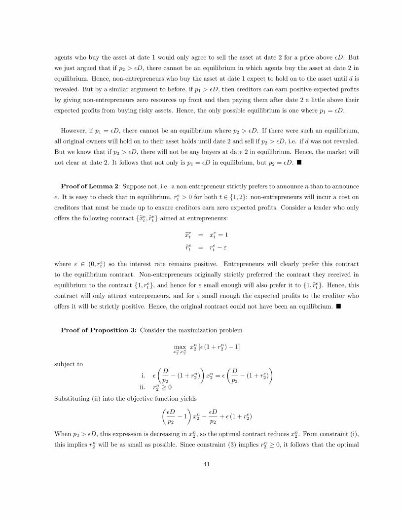
agents who buy the asset at date 1 would only agree to sell the asset at date 2 for a price above εD. But

we just argued that if p2 > εD, there cannot be an equilibrium in which agents buy the asset at date 2 in

equilibrium. Hence, non-entrepreneurs who buy the asset at date 1 expect to hold on to the asset until d is

revealed. But by a similar argument to before, if p1 > εD, then creditors can earn positive expected profits

by giving non-entrepreneurs zero resources up front and then paying them after date 2 a little above their

expected profits from buying risky assets. Hence, the only possible equilibrium is one where p1 = εD.

However, if p1 = εD, there cannot be an equilibrium where p2 > εD. If there were such an equilibrium,

all original owners will hold on to their asset holds until date 2 and sell if p2 > εD, i.e. if d was not revealed.

But we know that if p2 > εD, there will not be any buyers at date 2 in equilibrium. Hence, the market will

not clear at date 2. It follows that not only is p1 = εD in equilibrium, but p2 = εD. �

Proof of Lemma 2: Suppose not, i.e. a non-entrepreneur strictly prefers to announce n than to announce

e. It is easy to check that in equilibrium, ret > 0 for both t ∈ {1, 2}: non-entrepreneurs will incur a cost oncreditors that must be made up to ensure creditors earn zero expected profits. Consider a lender who only

offers the following contract {xet , ret } aimed at entrepreneurs:

xet = xet = 1

ret = ret − ε

where ε ∈ (0, ret ) so the interest rate remains positive. Entrepreneurs will clearly prefer this contract

to the equilibrium contract. Non-entrepreneurs originally strictly preferred the contract they received in

equilibrium to the contract {1, ret }, and hence for ε small enough will also prefer it to {1, ret }. Hence, thiscontract will only attract entrepreneurs, and for ε small enough the expected profits to the creditor who

offers it will be strictly positive. Hence, the original contract could not have been an equilibrium. �

Proof of Proposition 3: Consider the maximization problem

maxxn2 ,r

n2

xn2 [ε (1 + rn2 )− 1]

subject to

i. ε

(D

p2− (1 + rn2 )

)xn2 = ε

(D

p2− (1 + re2)

)ii. rn2 ≥ 0

Substituting (ii) into the objective function yields(εD

p2− 1)xn2 −

εD

p2+ ε (1 + re2)

When p2 > εD, this expression is decreasing in xn2 , so the optimal contract reduces xn2 . From constraint (i),

this implies rn2 will be as small as possible. Since constraint (3) implies rn2 ≥ 0, it follows that the optimal

41

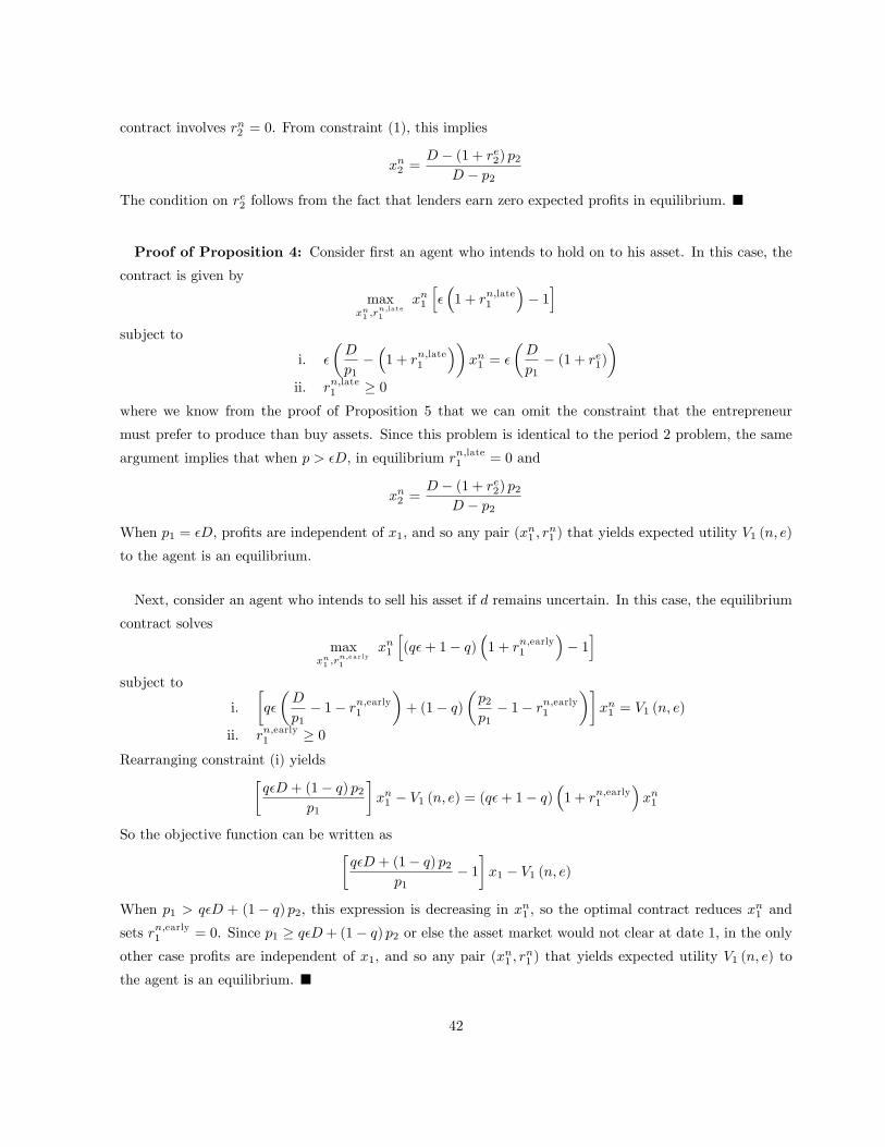
contract involves rn2 = 0. From constraint (1), this implies

xn2 =D − (1 + re2) p2

D − p2The condition on re2 follows from the fact that lenders earn zero expected profits in equilibrium. �

Proof of Proposition 4: Consider first an agent who intends to hold on to his asset. In this case, the

contract is given by

maxxn1 ,r

n,l a t e1

xn1

[ε(1 + rn,late1

)− 1]

subject to

i. ε

(D

p1−(1 + rn,late1

))xn1 = ε

(D

p1− (1 + re1)

)ii. rn,late1 ≥ 0

where we know from the proof of Proposition 5 that we can omit the constraint that the entrepreneur

must prefer to produce than buy assets. Since this problem is identical to the period 2 problem, the same

argument implies that when p > εD, in equilibrium rn,late1 = 0 and

xn2 =D − (1 + re2) p2

D − p2When p1 = εD, profits are independent of x1, and so any pair (xn1 , r

n1 ) that yields expected utility V1 (n, e)

to the agent is an equilibrium.

Next, consider an agent who intends to sell his asset if d remains uncertain. In this case, the equilibrium

contract solves

maxxn1 ,r

n,e a r ly1

xn1

[(qε+ 1− q)

(1 + rn,early1

)− 1]

subject to

i.[qε

(D

p1− 1− rn,early1

)+ (1− q)

(p2p1− 1− rn,early1

)]xn1 = V1 (n, e)

ii. rn,early1 ≥ 0Rearranging constraint (i) yields[

qεD + (1− q) p2p1

]xn1 − V1 (n, e) = (qε+ 1− q)

(1 + rn,early1

)xn1

So the objective function can be written as[qεD + (1− q) p2

p1− 1]x1 − V1 (n, e)

When p1 > qεD + (1− q) p2, this expression is decreasing in xn1 , so the optimal contract reduces xn1 andsets rn,early1 = 0. Since p1 ≥ qεD+ (1− q) p2 or else the asset market would not clear at date 1, in the onlyother case profits are independent of x1, and so any pair (xn1 , r

n1 ) that yields expected utility V1 (n, e) to

the agent is an equilibrium. �

42

 

 

 

 

 

 

 

 

 

 

 

 

 

Figure 1: Supply and demand in the asset market at t = 2 for I2 = ∅, 

assuming a single interest rate is charged to all borrowers at t = 1  

 

 

 

 

 

 

 

 

 

 

(a) 

 ЄD 

1

ЄD + (1‐Є)(1+r1)p1 

(b)

(c)

(d)

p2 

 

Shares of the 

risky asset 1‐n1/p1

n2/p2 

 

 

 

 

 

 

 

 

 

 

 

 

 

 

Figure 2: Supply and demand in the asset market at t = 2 for I2 = ∅, 

when some non‐entrepreneurs who buy at t = 1 sell at t = 2.  

 

 

 

 

 

 

 

 

 

ЄD 

1

ЄD + (1‐Є)(1+r1*)p1 

p2 

 

Shares of the 

risky asset 

ЄD + (1‐Є)(1+r1 )p1 *  

1‐n1/p1

n2/p2 

n2 

ЄD + (1‐Є)(1+r1*)p1 

 

 

 

 

 

 

   

 

 

 

 

 

 

 

 

 

 

 

 

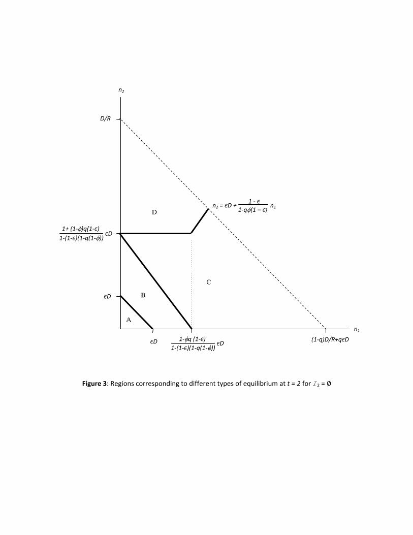
Figure 3: Regions corresponding to different types of equilibrium at t = 2 for I2 = ∅ 

 

 

 

 

 

ЄD  (1‐q)D/R+qЄD

A

B

C

D

D/R 

ЄD 

n1

n2 

n2 = ЄD +                      n11 ‐ Є 

1‐q(1 – Є) 

ЄD1‐q (1‐Є) 

1‐(1‐Є)(1‐q(1‐)) 

ЄD 1+ (1‐)q(1‐Є) 1‐(1‐Є)(1‐q(1‐)) 

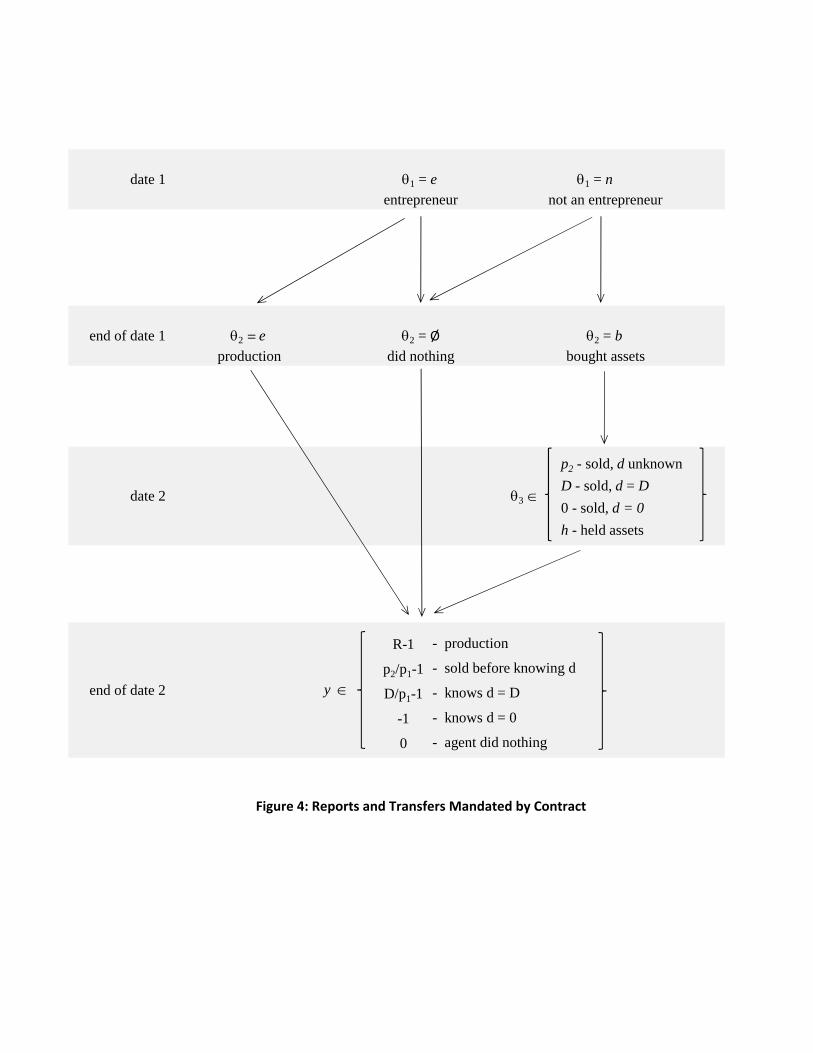
date 1 1 = e 1 = nentrepreneur not an entrepreneur

end of date 1 2 = e 2 = Ø 2 = bproduction did nothing bought assets

date 2 3 œ

end of date 2 y œ

Figure 4: Reports and Transfers Mandated by Contract

p2 - sold, d unknownD - sold, d = D0 - sold, d = 0

h - held assets

R-1

p2/p1-1

D/p1-1

-1

0

- production

- sold before knowing d

- knows d = D

- knows d = 0

- agent did nothing

 

 

 

 

 

 

 

 

 

 

 

 

 

 

 

 

 

 

 

 

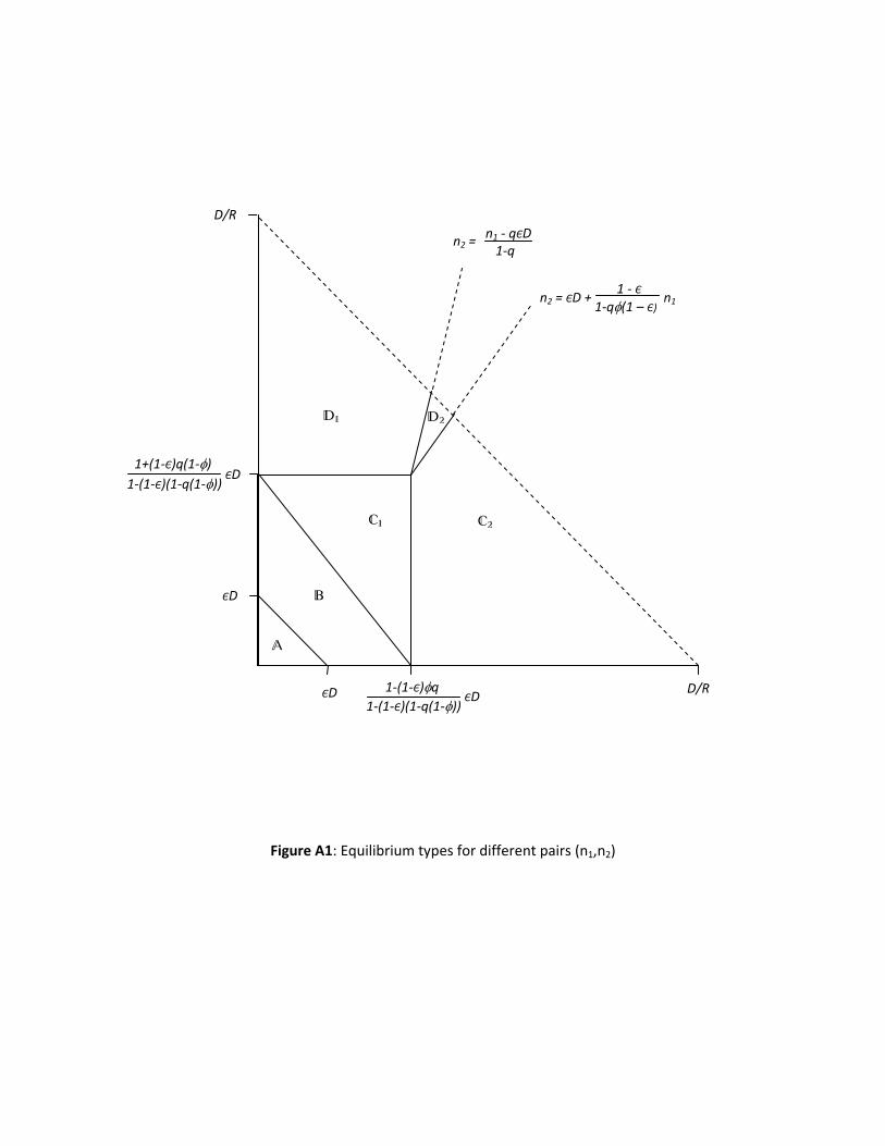
Figure A1: Equilibrium types for different pairs (n1,n2) 

ЄD  D/R 

A

B

C1

C2

D1

D2

D/R 

ЄD 

ЄD 1+(1‐Є)q(1‐) 

1‐(1‐Є)(1‐q(1‐)) 

ЄD 1‐(1‐Є)q 

1‐(1‐Є)(1‐q(1‐)) 

n2 = n1 ‐ qЄD1‐q

n2 = ЄD +                      n1 1 ‐ Є 

1‐q(1 – Є) 

References

[1] Albagli, Elias, Christian Hellwig, and Aleh Tsyvinski, 2011. “A Theory of Asset Prices Based on

Heterogeneous Information" Cowles Foundation Discussion Papers 1827, Yale University.

[2] Allen, Franklin and Gary Gorton, 1993. “Churning Bubbles”Review of Economic Studies, 60(4), Oc-

tober, p813-836.

[3] Allen, Franklin and Douglas Gale, 1994.“Limited Market Participation and Volatility of Asset Prices”

American Economic Review, 84(4), September, p933-55.

[4] Allen, Franklin and Douglas Gale, 2000. “Bubbles and Crises”Economic Journal, 110(460), January,

p236-255.

[5] Allen, Franklin, Stephen Morris, and Andrew Postlewaite, 1993. “Finite Bubbles with Short Sales

Constraints and Asymmetric Information”Journal of Economic Theory, 61(2), December, p206-29.

[6] Barlevy, Gadi and Jonas Fisher, 2012. “Mortgage Choice and Housing Speculation”Federal Reserve

Bank of Chicago Working Paper.

[7] Bewley, Truman, 1980. “The Optimum Quantity of Money”Models of Monetary Economics, eds. J.

Kareken and N. Wallace. Minneapolis, Minnesota: Federal Reserve Bank, p169-210.

[8] Blanchard, Olivier and Mark Watson, 1982. “Bubbles, Rational Expectations, and Financial markets”

Crisis in the Economic and Financial Structure: Bubbles, Bursts, and Shocks, ed. P. Wachtel. Lexing-

ton, Massachusetts: Lexington Books, p295—315.

[9] Burnside, Craig, Martin Eichenbaum, and Sergio Rebelo, 2011. “Understanding Booms and Busts in

Housing Markets”Mimeo, Northwestern University.

[10] Caballero, Ricardo and Arvind Krishnamurthy, 2006. “Bubbles and Capital Flow Volatility: Causes

and Risk Management”Journal Monetary of Economics, 53(1), January, p35-53.

[11] Colon, John, 2004. “Simple Finite Horizon Bubbles Robust to Higher Order Knowledge”Econometrica,

72(3), p927-936.

[12] Diamond, Peter, 1965. “National Debt in a Neoclassical Growth Model”American Economic Review,

55(5), Part 1, December, p1126-50.

[13] Diba, Behzad and Herschel Grossman, 1987. “On the Inception of Rational Bubbles”Quarterly Journal

of Economics, 102(3), August, p697-700.

[14] Eraker, Bjorn and Mark Ready, 2013. “Do Investors Overpay for Stocks with Lottery-Like Payoffs? An

Examination of the Returns on OTC Stocks”Mimeo, University of Wisconsin.

43

[15] Farhi, Emmanuel and Jean Tirole, 2011. “Bubbly Liquidity”Review of Economics Studies, forthcoming.

[16] Gale, Douglas and Martin Hellwig, 1985. “Incentive-Compatible Debt Contracts: The One-Period

Problem”Review of Economic Studies, 52(4), October, p647-63.

[17] Geanakpolos, John, 2010. “The Leverage Cycle”NBER Macroeconomics Annual, 24(1), p1-66.

[18] Harrison, Michael and David Kreps, 1978. “Speculative Investor Behavior in a Stock Market with

Heterogeneous Expectations”Quarterly Journal of Economics, 92(2), May, p323-36.

[19] Hong, Harrison and David Sraer, 2011. “Quiet Bubbles”Mimeo, Princeton University

[20] Kocherlakota, Narayana, 1992. “Bubbles and Constraints on Debt Accumulation”Journal of Economic

Theory, 57 (1), p245– 56

[21] Mimra, Wanda and AchimWambach, 2011. “A Game-Theoretic Foundation for the Wilson Equilibrium

in Competitive Insurance Markets with Adverse Selection”CESifo Working Paper 3412.

[22] Miyazaki, Hajime, 1977, “The Rat Race and Internal Labor Markets", Bell Journal of Economics,

8(2), p394-418.

[23] Netzer, Nick and Florian Scheuer, 2013. A Game Theoretic Foundation of Competititve Equilibria

with Adverse Selection. Stanford University working paper and forthcoming, International Economic

Review.

[24] Rocheteau, Guillaume and Randall Wright, 2011. “Liquidity and Asset Market Dynamics”Mimeo,

University of Wisconsin.

[25] Rothschild, M., Stiglitz, J., 1976. “Equilibrium in Competitive Insurance Markets: An Essay on the

Economics of Imperfect Information.”Quarterly Journal of Economics, 90 (4), p629—649.

[26] Samuelson, Paul, 1958. “An Exact Consumption-Loan Model of Interest with or without the Social

Contrivance of Money”Journal of Political Economy, 66, p467-82.

[27] Santos, Manuel and Michael Woodford, 1997. “Rational Asset Pricing Bubbles”Econometrica, 65(1),

January, p19-57.

[28] Spence, Michael, 1978. “Product Differentiation and Performance in Insurance Markets", Journal of

Public Economics, 10(3), p427-447.

[29] Temin, Peter and Hans-Joachim Voth, 2004. “Riding the South Sea Bubble” American Economic

Review , 94 (5), December, p1654-1668.

[30] Tirole, Jean, 1985. “Asset Bubbles and Overlapping Generations” Econometrica, 53(6), November,

p1499-1528.

44

[31] Townsend, Robert, 1979. “Optimal Contracts and Competitive Markets with Costly State Verification”

Journal of Economic Theory, 21, p265—93.

[32] Wilson, Charles, 1977. “A Model of Insurance Markets with Incomplete Information.” Journal of

Economic Theory, 16 (2), p167—207.

45

1

Working Paper Series

A series of research studies on regional economic issues relating to the Seventh Federal Reserve District, and on financial and economic topics.

A Leverage-based Model of Speculative Bubbles WP-08-01 Gadi Barlevy Displacement, Asymmetric Information and Heterogeneous Human Capital WP-08-02 Luojia Hu and Christopher Taber BankCaR (Bank Capital-at-Risk): A credit risk model for US commercial bank charge-offs WP-08-03 Jon Frye and Eduard Pelz Bank Lending, Financing Constraints and SME Investment WP-08-04 Santiago Carbó-Valverde, Francisco Rodríguez-Fernández, and Gregory F. Udell Global Inflation WP-08-05 Matteo Ciccarelli and Benoît Mojon Scale and the Origins of Structural Change WP-08-06 Francisco J. Buera and Joseph P. Kaboski Inventories, Lumpy Trade, and Large Devaluations WP-08-07 George Alessandria, Joseph P. Kaboski, and Virgiliu Midrigan School Vouchers and Student Achievement: Recent Evidence, Remaining Questions WP-08-08 Cecilia Elena Rouse and Lisa Barrow Does It Pay to Read Your Junk Mail? Evidence of the Effect of Advertising on Home Equity Credit Choices WP-08-09 Sumit Agarwal and Brent W. Ambrose

The Choice between Arm’s-Length and Relationship Debt: Evidence from eLoans WP-08-10 Sumit Agarwal and Robert Hauswald

Consumer Choice and Merchant Acceptance of Payment Media WP-08-11 Wilko Bolt and Sujit Chakravorti Investment Shocks and Business Cycles WP-08-12 Alejandro Justiniano, Giorgio E. Primiceri, and Andrea Tambalotti New Vehicle Characteristics and the Cost of the Corporate Average Fuel Economy Standard WP-08-13 Thomas Klier and Joshua Linn Realized Volatility WP-08-14 Torben G. Andersen and Luca Benzoni Revenue Bubbles and Structural Deficits: What’s a state to do? WP-08-15 Richard Mattoon and Leslie McGranahan

2

Working Paper Series (continued) The role of lenders in the home price boom WP-08-16 Richard J. Rosen Bank Crises and Investor Confidence WP-08-17 Una Okonkwo Osili and Anna Paulson Life Expectancy and Old Age Savings WP-08-18 Mariacristina De Nardi, Eric French, and John Bailey Jones Remittance Behavior among New U.S. Immigrants WP-08-19 Katherine Meckel Birth Cohort and the Black-White Achievement Gap: The Roles of Access and Health Soon After Birth WP-08-20 Kenneth Y. Chay, Jonathan Guryan, and Bhashkar Mazumder Public Investment and Budget Rules for State vs. Local Governments WP-08-21 Marco Bassetto Why Has Home Ownership Fallen Among the Young? WP-09-01 Jonas D.M. Fisher and Martin Gervais Why do the Elderly Save? The Role of Medical Expenses WP-09-02 Mariacristina De Nardi, Eric French, and John Bailey Jones Using Stock Returns to Identify Government Spending Shocks WP-09-03 Jonas D.M. Fisher and Ryan Peters Stochastic Volatility WP-09-04 Torben G. Andersen and Luca Benzoni The Effect of Disability Insurance Receipt on Labor Supply WP-09-05 Eric French and Jae Song CEO Overconfidence and Dividend Policy WP-09-06 Sanjay Deshmukh, Anand M. Goel, and Keith M. Howe Do Financial Counseling Mandates Improve Mortgage Choice and Performance? WP-09-07 Evidence from a Legislative Experiment Sumit Agarwal,Gene Amromin, Itzhak Ben-David, Souphala Chomsisengphet, and Douglas D. Evanoff Perverse Incentives at the Banks? Evidence from a Natural Experiment WP-09-08 Sumit Agarwal and Faye H. Wang Pay for Percentile WP-09-09 Gadi Barlevy and Derek Neal The Life and Times of Nicolas Dutot WP-09-10 François R. Velde Regulating Two-Sided Markets: An Empirical Investigation WP-09-11 Santiago Carbó Valverde, Sujit Chakravorti, and Francisco Rodriguez Fernandez

3

Working Paper Series (continued) The Case of the Undying Debt WP-09-12 François R. Velde Paying for Performance: The Education Impacts of a Community College Scholarship Program for Low-income Adults WP-09-13 Lisa Barrow, Lashawn Richburg-Hayes, Cecilia Elena Rouse, and Thomas Brock Establishments Dynamics, Vacancies and Unemployment: A Neoclassical Synthesis WP-09-14 Marcelo Veracierto The Price of Gasoline and the Demand for Fuel Economy: Evidence from Monthly New Vehicles Sales Data WP-09-15 Thomas Klier and Joshua Linn Estimation of a Transformation Model with Truncation, Interval Observation and Time-Varying Covariates WP-09-16 Bo E. Honoré and Luojia Hu Self-Enforcing Trade Agreements: Evidence from Antidumping Policy WP-09-17 Chad P. Bown and Meredith A. Crowley Too much right can make a wrong: Setting the stage for the financial crisis WP-09-18 Richard J. Rosen Can Structural Small Open Economy Models Account for the Influence of Foreign Disturbances? WP-09-19 Alejandro Justiniano and Bruce Preston Liquidity Constraints of the Middle Class WP-09-20 Jeffrey R. Campbell and Zvi Hercowitz Monetary Policy and Uncertainty in an Empirical Small Open Economy Model WP-09-21 Alejandro Justiniano and Bruce Preston Firm boundaries and buyer-supplier match in market transaction: IT system procurement of U.S. credit unions WP-09-22 Yukako Ono and Junichi Suzuki Health and the Savings of Insured Versus Uninsured, Working-Age Households in the U.S. WP-09-23 Maude Toussaint-Comeau and Jonathan Hartley The Economics of “Radiator Springs:” Industry Dynamics, Sunk Costs, and Spatial Demand Shifts WP-09-24 Jeffrey R. Campbell and Thomas N. Hubbard On the Relationship between Mobility, Population Growth, and Capital Spending in the United States WP-09-25 Marco Bassetto and Leslie McGranahan The Impact of Rosenwald Schools on Black Achievement WP-09-26 Daniel Aaronson and Bhashkar Mazumder

4

Working Paper Series (continued) Comment on “Letting Different Views about Business Cycles Compete” WP-10-01 Jonas D.M. Fisher Macroeconomic Implications of Agglomeration WP-10-02 Morris A. Davis, Jonas D.M. Fisher and Toni M. Whited Accounting for non-annuitization WP-10-03 Svetlana Pashchenko Robustness and Macroeconomic Policy WP-10-04 Gadi Barlevy Benefits of Relationship Banking: Evidence from Consumer Credit Markets WP-10-05 Sumit Agarwal, Souphala Chomsisengphet, Chunlin Liu, and Nicholas S. Souleles The Effect of Sales Tax Holidays on Household Consumption Patterns WP-10-06 Nathan Marwell and Leslie McGranahan Gathering Insights on the Forest from the Trees: A New Metric for Financial Conditions WP-10-07 Scott Brave and R. Andrew Butters Identification of Models of the Labor Market WP-10-08 Eric French and Christopher Taber Public Pensions and Labor Supply Over the Life Cycle WP-10-09 Eric French and John Jones Explaining Asset Pricing Puzzles Associated with the 1987 Market Crash WP-10-10 Luca Benzoni, Pierre Collin-Dufresne, and Robert S. Goldstein Prenatal Sex Selection and Girls’ Well‐Being: Evidence from India WP-10-11 Luojia Hu and Analía Schlosser Mortgage Choices and Housing Speculation WP-10-12 Gadi Barlevy and Jonas D.M. Fisher Did Adhering to the Gold Standard Reduce the Cost of Capital? WP-10-13 Ron Alquist and Benjamin Chabot Introduction to the Macroeconomic Dynamics: Special issues on money, credit, and liquidity WP-10-14 Ed Nosal, Christopher Waller, and Randall Wright Summer Workshop on Money, Banking, Payments and Finance: An Overview WP-10-15 Ed Nosal and Randall Wright Cognitive Abilities and Household Financial Decision Making WP-10-16 Sumit Agarwal and Bhashkar Mazumder Complex Mortgages WP-10-17 Gene Amromin, Jennifer Huang, Clemens Sialm, and Edward Zhong

5

Working Paper Series (continued) The Role of Housing in Labor Reallocation WP-10-18 Morris Davis, Jonas Fisher, and Marcelo Veracierto Why Do Banks Reward their Customers to Use their Credit Cards? WP-10-19 Sumit Agarwal, Sujit Chakravorti, and Anna Lunn The impact of the originate-to-distribute model on banks before and during the financial crisis WP-10-20 Richard J. Rosen Simple Markov-Perfect Industry Dynamics WP-10-21 Jaap H. Abbring, Jeffrey R. Campbell, and Nan Yang Commodity Money with Frequent Search WP-10-22 Ezra Oberfield and Nicholas Trachter Corporate Average Fuel Economy Standards and the Market for New Vehicles WP-11-01 Thomas Klier and Joshua Linn The Role of Securitization in Mortgage Renegotiation WP-11-02 Sumit Agarwal, Gene Amromin, Itzhak Ben-David, Souphala Chomsisengphet, and Douglas D. Evanoff Market-Based Loss Mitigation Practices for Troubled Mortgages Following the Financial Crisis WP-11-03 Sumit Agarwal, Gene Amromin, Itzhak Ben-David, Souphala Chomsisengphet, and Douglas D. Evanoff Federal Reserve Policies and Financial Market Conditions During the Crisis WP-11-04 Scott A. Brave and Hesna Genay The Financial Labor Supply Accelerator WP-11-05 Jeffrey R. Campbell and Zvi Hercowitz Survival and long-run dynamics with heterogeneous beliefs under recursive preferences WP-11-06 Jaroslav Borovička A Leverage-based Model of Speculative Bubbles (Revised) WP-11-07 Gadi Barlevy