58 Zakaria, Journal of International and Global Economic Studies, 7(1), June 2014, 58-81

Imperfection of Credit Markets, Speculative Bubbles and

Financial Accelerator in Morocco

Firano Zakaria

University Mohammed V Rabat-Agdal

Abstract : The credit market continues to be the main mechanism for financing investments in

developing countries, particularly in Morocco. In this sense, monetary and macro-prudential

policies require the inclusion of this market in macroeconomic analysis. In this article, we use

the model proposed by Bernanke et al. (1999) "BGG" in the case of Morocco to answer two

main questions: is there a mechanism for financial accelerator in Morocco, according to which

macroeconomic shocks can be amplified and lead to greater instability of the macroeconomic

framework. In a second step, we propose a new monetary rule, taking into account changes in

asset prices and the possibility of speculative bubbles in Morocco. The results argue that credit

market imperfections in Morocco amplify macroeconomic shocks and affirm the hypothesis of

the existence of financial accelerator in Morocco. In addition, the counterfactual analysis shows

that the Taylor rule augmented with asset prices provides greater economic stability.

Keywords: financial accelerator, rational bubbles, financial frictions.

JEL Classification: D53, E44

1. Introduction

The model of new macroeconomic synthesis were widely considering that the financial

activities do not affect the real economy. It is obvious, when one considers that the financial

sector, which plays the role of intermediation, can create value and therefore affect the price

formation. Fisher (1933) and Keynes (1929) were the first to consider the boom (or cycles) in

the financial markets may adversely reflect on the real economy. However, macroeconomic

models have always overlooked this design by choosing a real doctrine.

Thus, a model that describes effectiveness the reality of economy must be able to include any

component that may impact the price formation as well as economic growth. In this perspective,

the model of Bernanke et al. (1998, 1999) aimed to ensure that imperfections in financial

markets, especially the credit market, can be easily incorporated into macroeconomic models.

In addition, their development at a macroeconomic framework improves the perception of all

economic policies and provides a framework for analyzing more realistic and adapted to better

decision making.

In the same view, integration of credit markets in macroeconomic models can incorporate a

significant financial friction’s which often faces borrowers. Certainly, the perfection of the

market ensures optimality allocation of savings into productive investment, however, the

existence of imperfection (rationale financial frictions) supports the need for have financial

intermediaries that can provide an additional profit of information there by reducing friction

and to ensure optimal loan contracts and borrowing (Diamond et al (1983)).

59

Beyond the desire to describe the reality of the economy (the existence of financial

intermediation), the introduction of the credit market in macroeconomic models used to insert

the credit frictions in a traditional cyclical analysis. It is able to improve the analysis of cycles

and also to achieve a better explanation of macro financial evolution. In other words, the

existence of these frictions on the credit market may have significant effects on the behavior of

macroeconomic variables, in particular on the economic cycle. As indicated in Bernanke et al.

(1998) in the BGG model, financial frictions significantly impacting economic cycles and can

cause deformation of the prices. In other words, monetary policy and productivity shocks, even

when they are quite small, can have important consequences when there are financial frictions

on the credit market.

The introduction of the credit market (financial frictions) can also provide an appropriate

framework for formulating empirical answers concerning the problem of the choice of the

optimal structure (Modigliani et al. (1954), “MM”). In the sense that the existence of financial

frictions on the credit market can’t make sense of the MM theorem from which the value of the

firm is independent of its financial structure.

In this context, the introduction of frictions on the credit market can put forward a concept of

financial accelerator (Bernanke et al. (1999)), which can amplify and propagate macroeconomic

shocks. The financial accelerator stems from the existence of the choice between internal

financing and external financing which is in function of the risk premium (the difference

between expected return and cost of capital) and collateral of borrowing firms. In this context

and when market imperfections are already taken into account, borrowers tend, if there is a low

flow to use a financial intermediary, which massively increases the agency costs. In this context,

the banks should demand more profitability to satisfy all requirements of the internal and

external financing.

In this respect, and in an environment of asymmetric information, the risk premium is inversely

related to the net value of the firm. Indeed, when the value of the firm increases the risk

premium decreases due to the presence of a low exploitation risk and also because of the

behavior of investors and banks. When investors have little money to invest in a particular

project the use of financial intermediary becomes a necessity, however, this ability involves the

occurrence of a conflict of interest between the two parties (agency problem), which results in

an increase in agency costs thereby increasing the risk premium.

At equilibrium, the lenders are required for higher costs by seeking a higher return. As such,

external funding is pro-cyclical in reason to the pro-cyclicality of profits and asset prices, while

the risk premium is countercyclical weighing negatively on the loan and therefore in investment

and spending production.

The inclusion of financial frictions on the credit market does not entail much loss of relevance

in terms of analysis of stabilization policies. In contrast, the framework also allows taking into

account issues related to nominal and real rigidities. Thus, the framework presented in this work

takes into account the relationship between asset prices and investment and productive

heterogeneity between firms.

This paper presents a model with financial frictions on the credit market in Morocco. The goal

is to confirm that financial frictions in the credit market have a significant impact on the degree

of propagation of shocks. In other words, the existence of agency problems related to the

presence of financial intermediation is ahead the phenomenon of financial accelerator. In

addition, the paper presents a new augmented Taylor rule for the case of Morocco, to stabilize

the macroeconomic framework in the presence of speculative bubbles and therefore achieve a

goal of financial stability. The next section shows how we can integrate financial frictions in

function optimization companies and all economic agents involved. The second section

60

develops the log-linear model that will be used in estimation. The following section describes

how bubbles can be integrated into a macroeconomic rational framework. The final section

presents the results obtained.

2. Financial Frictions and Economic Sectors

The introduction of financial frictions in a new Keynesian (NKM), requires all of the

relationships surrounding lending and borrowing between private agents take place in a

framework of macroeconomic equilibrium. In this sense, it is important to review the way in

which we define the heterogeneity among agents. Then, to allow better integration of financial

frictions on the credit market, it is essential to use a new reading of financial contracts between

private agents to integrate the logic of financing through the use of mediation financial. The

following developments are only interested in the second track trying to integrate a new design

of financial contracts including the use of external financing in a manner to maintain the

relevance of the balance of the financial structure of private agents, without the need to expand

the heterogeneity of agents.

In light of these developments, the model presented here is based on the work of Bernanke et

al. (1999) and to integrate and assess the role of financial frictions in macroeconomic modeling

framework to the case of Morocco. The model is composed of three types of economic agents

namely, households, entrepreneur, retailers, the central bank and the fiscal authorities. The

distinction between entrepreneurs and retailers need to take into account the rigidity of prices

for at least the agents “price-maker”. Thus, we assume that there is perfect competition in which

entrepreneurs produce goods and sell them to retailers who sell them in a monopolistic market,

which give them power over prices.

To incorporate financial frictions in this framework, we assume that entrepreneurs have a finite

lifetime on the horizon of a period. This allows assuming that there is a continuous renewal of

investment projects (firms) able to reject the hypothesis that the corporate sector can accumulate

enough cash flow, leaving disappear external financing. In addition, this assumption facilitates

the aggregation of entrepreneurs and limits their number (constant) companies over a period.

Thus, in each period entrepreneurs acquire production equipment (only new firms have the

opportunity to acquire these investments, firms continue to use their existing capital

accumulated beyond). These investments are used to produce the work, according to a given

technology, final goods, using a self-funding and / or a loan from a financial intermediary.

The net worth of entrepreneurs is assumed to be two sources namely: benefits and their own

work. This value plays an important role in the choice of financing and the use of external

financing in particular. Thus, very colossal values are an important source of cash flow and

little discouraged borrower’s recourse to external funds, which significantly reduces the risk

premium.

The existence of a risk premium is argued by a simple agency problem (see above). In this

regard, the financial contract must be developed to the extent that it allows limited risk premium

by reducing conflicts of interest and potential agency costs.

To integrate all of these arguments in a macroeconomic model, it is necessary to proceed in two

steps: first time use a redefinition of the functions of entrepreneurial behavior to integrate their

use of funding from external to a financial intermediary and a second time to include these

results in a new Keynesian. In this sense, the result would be to assess the impact of using

funding exogenous macroeconomic stability and its effect on the propagation and amplification

of shocks.

61

2.1. Optimal structure of capital: Modigliani and Miller have false?

Investment decision at the firm (production) is related to the level of capital required and also

the rate of return expected. In this perspective, the expected rate of return and capital are

endogenous variables within the macroeconomic framework of the proposed model.

It is considered that the time « t» the contractor acquires capital (Kt+1) for possible use at the

time « t+1 » .The price will be spent on the acquisition of a unit of capital is denoted (Qt+1).

The return on investment is sensitive to two types of risk including: systemic risk and

idiosyncratic risk. The first type is common to all firms, while the second is related to factors

specific to the company. Operating in an equilibrium framework only specific risk is

considered. To this end, the profitability of the company at the time « t+1 » is ω*RKt+1, ω is

with the idiosyncratic risk factor which the process is i.i.d. and the distribution function is

positive with an expected equal to unity.

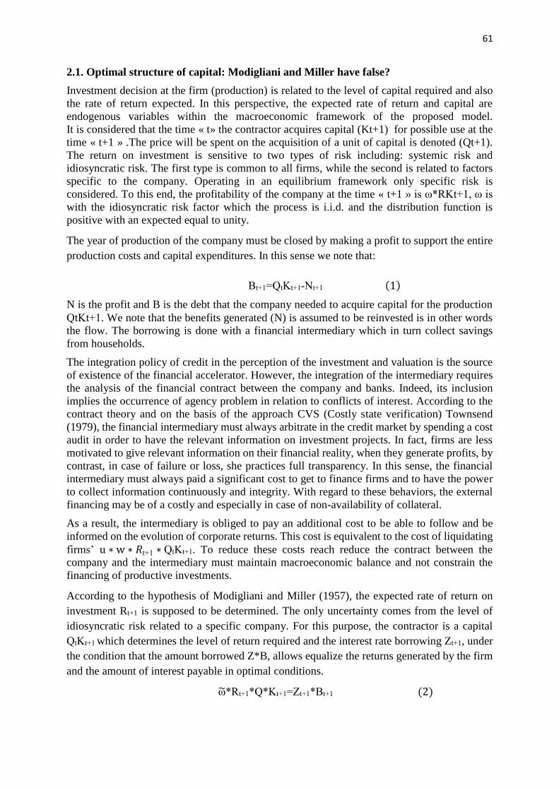
The year of production of the company must be closed by making a profit to support the entire

production costs and capital expenditures. In this sense we note that:

Bt+1=QtKt+1-Nt+1 (1)

N is the profit and B is the debt that the company needed to acquire capital for the production

QtKt+1. We note that the benefits generated (N) is assumed to be reinvested is in other words

the flow. The borrowing is done with a financial intermediary which in turn collect savings

from households.

The integration policy of credit in the perception of the investment and valuation is the source

of existence of the financial accelerator. However, the integration of the intermediary requires

the analysis of the financial contract between the company and banks. Indeed, its inclusion

implies the occurrence of agency problem in relation to conflicts of interest. According to the

contract theory and on the basis of the approach CVS (Costly state verification) Townsend

(1979), the financial intermediary must always arbitrate in the credit market by spending a cost

audit in order to have the relevant information on investment projects. In fact, firms are less

motivated to give relevant information on their financial reality, when they generate profits, by

contrast, in case of failure or loss, she practices full transparency. In this sense, the financial

intermediary must always paid a significant cost to get to finance firms and to have the power

to collect information continuously and integrity. With regard to these behaviors, the external

financing may be of a costly and especially in case of non-availability of collateral.

As a result, the intermediary is obliged to pay an additional cost to be able to follow and be

informed on the evolution of corporate returns. This cost is equivalent to the cost of liquidating

firms’ u ∗ w ∗ 𝑅t+1 ∗ QtKt+1. To reduce these costs reach reduce the contract between the

company and the intermediary must maintain macroeconomic balance and not constrain the

financing of productive investments.

According to the hypothesis of Modigliani and Miller (1957), the expected rate of return on

investment Rt+1 is supposed to be determined. The only uncertainty comes from the level of

idiosyncratic risk related to a specific company. For this purpose, the contractor is a capital

QtKt+1 which determines the level of return required and the interest rate borrowing Zt+1, under

the condition that the amount borrowed Z*B, allows equalize the returns generated by the firm

and the amount of interest payable in optimal conditions.

ω̃*Rt+1*Q*Kt+1=Zt+1*Bt+1 (2)

62

The optimal level of idiosyncratic risk ω̃ to equalize the performance of the company with the

requirements of the financial intermediary. If ω̃ > ω the contractor cannot meet its own

commitments vis-à-vis donors receive the amount (1 − 𝑢) 𝜔𝑅t+1QtKt+1. However, in the

reverse situation, the contractor can make a profit to cope with different commitments and also

identified additional profits.

In this sense, the financial intermediary therefore requires an additional cost from the contractor

to finance its projects, this cost can be written as follows:

[1 − 𝐹(�̃�)]𝑍𝑡+1𝑗

𝐵𝑡+1𝑗

+ (1 − 𝑢) ∫ 𝜔𝑅𝑡+1𝑄𝑡𝐾𝑡+1d𝐹(𝜔)∞

0

= 𝑅𝑡+1𝐵𝑡+1 (3)

The right side of the equation represents the opportunity cost and the left when it is on the cost

required by the borrower. This last part is divided into two: the cost of liquidation and the

repayment of principal. If we replace Z by its value to find the requirement of donors based on

specific risk, we can write have the following equivalence:

{[1 − 𝐹(�̃�)]�̃� + (1 − 𝑢) ∫ ωdF(ω)Rt+1

QtK

t+1dF(ω)

∞

0

} Rt+1

QtK

t+1=R

t+1(Q

tK

t+1− 𝑁𝑡) (4)

with 𝐹(�̃�) is the enterprise default rate.

In cases where the level of ω is not acceptable and pose a risk to inerent borrowing activity. In

this perspective, the company is unable to honor its commitments vis-à-vis the financial

intermediary. This denier would be able to take credit rationing1.

On the basis of its developments and considering the expected returns are determined, in this

case we can write the profitability of the project the contractor as follows:

𝐸 {∫ 𝜔𝑅𝑡+1𝑄𝑡𝐾𝑡+1𝑑𝐹(𝜔)∞

0

−(1 − 𝐹(�̃�))�̃�𝑅𝑡+1𝑄𝑡𝐾𝑡+1} (5)

By combining the expected return with the requirement of financial intermediary found the

following relationship:

𝐸 {[1 − 𝑢 ∫ 𝑑𝐹(𝜔)�̃�

0

] 𝑈𝑡+1𝑟𝑘 } 𝐸{𝑅𝑡+1

𝑘 }𝑄𝑡𝐾𝑡+1 − 𝑅𝑡+1(𝑄𝑡𝐾𝑡+1 − 𝑁𝑡+1) (6)

Knowing that 𝑈𝑡+1𝑟𝑘 = 𝑅𝑡+1

𝑘 /𝐸{𝑅𝑡+1𝑘 } is the completion rate of return from its conditional

expectation. If we denote the discount rate of return on capital is 𝑠 = 𝐸{𝑅𝑡+1𝑘 /𝑅𝑡+1} whose

value is greater than 1, in this case the optimal condition for d 'buy capital in the financial

intermediary:

𝑄𝑡𝐾𝑡+1 = 𝜗(𝑠)𝑁𝑡+1 (7)

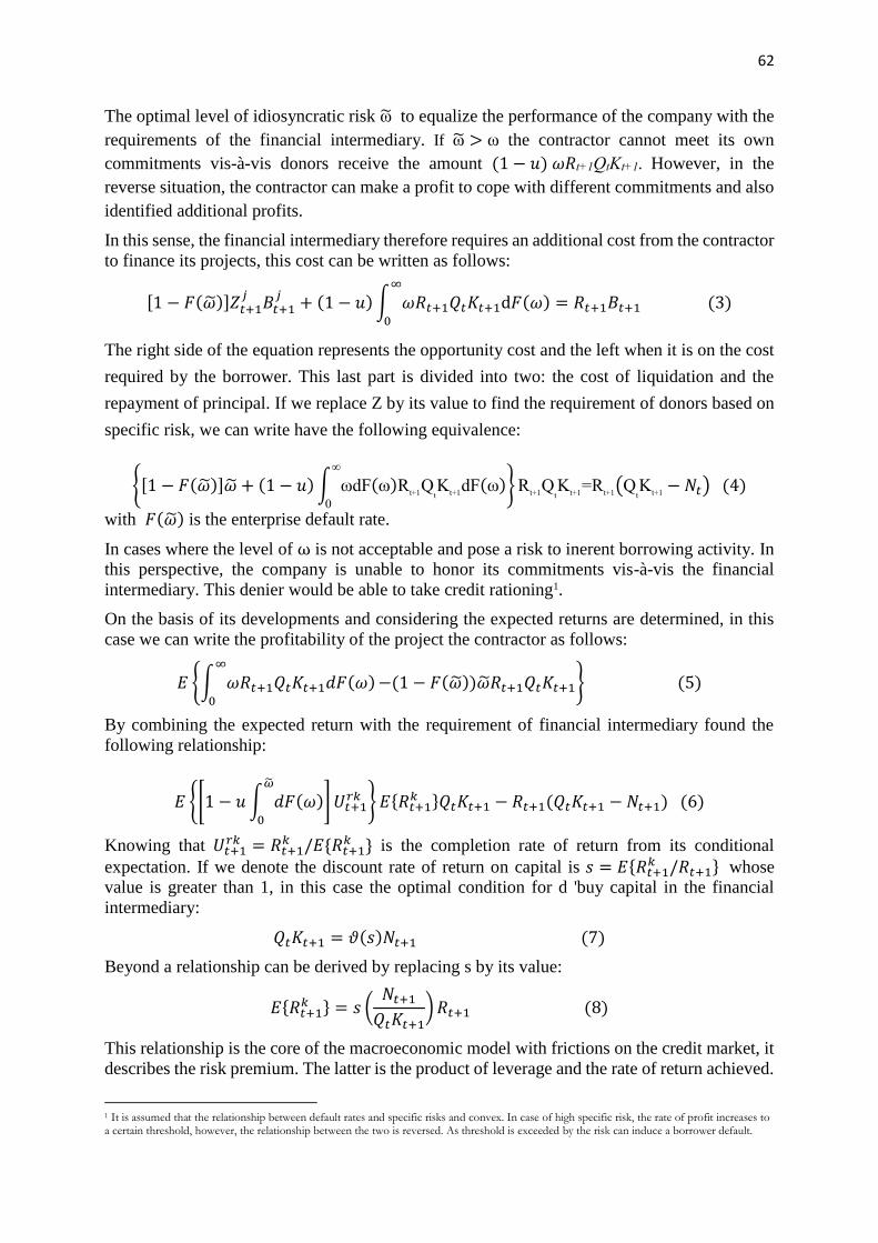
Beyond a relationship can be derived by replacing s by its value:

𝐸{𝑅𝑡+1𝑘 } = 𝑠 (

𝑁𝑡+1

𝑄𝑡𝐾𝑡+1) 𝑅𝑡+1 (8)

This relationship is the core of the macroeconomic model with frictions on the credit market, it

describes the risk premium. The latter is the product of leverage and the rate of return achieved.

1 It is assumed that the relationship between default rates and specific risks and convex. In case of high specific risk, the rate of profit increases to a certain threshold, however, the relationship between the two is reversed. As threshold is exceeded by the risk can induce a borrower default.

63

If you equity financing only (flow) rate of return is equal to the expected rate of return achieved

is the optimality condition if no contract of financial intermediation.

After defining how the integration of external financing must change the behavior of

entrepreneurs and the definition of the notion of risk premium which is the core of the financial

accelerator. We present thereafter the equilibrium conditions of the various economic agents

and their objective functions.

2.2. The entrepreneur sector

The agency problem between the lender and the borrower will be included in a general

equilibrium framework for improving the standard DSGE model for the case of Morocco. The

innovation relates to the integration of financial frictions on the credit market resulting from

the optimality under the contract between donors and contractors, is due to the existence of

agency costs.

Changes to the model are considered for endogenous the cost of capital of the company and

also the expected return of investment projects, taking into account costs related to the use of

bank credit.

Sector entrepreneurs acquire capital in each period and consist of two components: capital and

labor:

𝑌𝑡 = 𝐴𝑡𝐾𝑡𝛼𝐿𝑡

1−𝛼 (9)

If you consider that I was spending in terms of capital, then we can write:

𝐾𝑡+1 = 𝜃 (𝐼𝑡

𝐾𝑡) 𝐾𝑡 + (1 − 𝜎)𝐾𝑡 (10)

With 𝜎 is the rate of depreciation of the capital.

To allow the price to be variable and also to make endogenous considering, according to the

approach of Kiyotoki et al. (1997), as:

𝑄𝑡 =1

[𝜃′ (𝐼𝑡

𝐾𝑡)]

(11)

By assumption we note that the cost of production in intermediate 1/X, equivalently X is

considered the mark-up of the monopoly. In this case the rent to pay for a unit of capital is equal

to:

1

𝑋𝑡+1∗

𝛾𝑌𝑡+1

𝐾𝑡+1 (12)

Thus, profitability can be written as follows:

𝐸{𝑅𝑡+1𝑘 } =

1𝑋𝑡+1

∗𝛾𝑌𝑡+1

𝐾𝑡+1+ 𝑄𝑡+1(1 − 𝜎)

𝑄𝑡 (13)

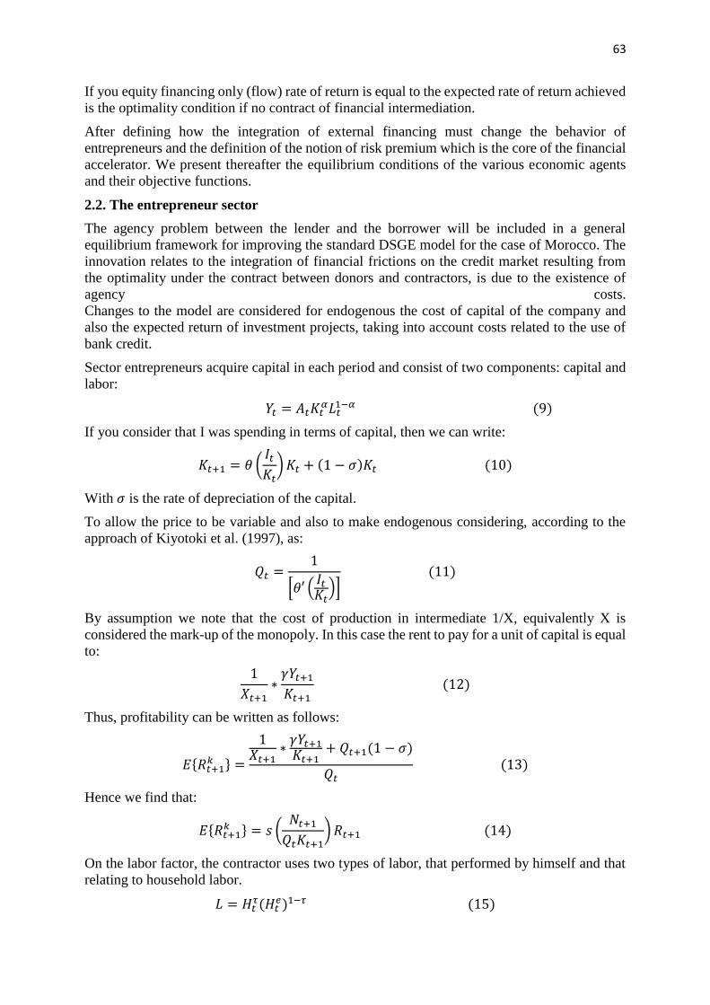
Hence we find that:

𝐸{𝑅𝑡+1𝑘 } = 𝑠 (

𝑁𝑡+1

𝑄𝑡𝐾𝑡+1) 𝑅𝑡+1 (14)

On the labor factor, the contractor uses two types of labor, that performed by himself and that

relating to household labor.

𝐿 = 𝐻𝑡𝜏(𝐻𝑡

𝑒)1−𝜏 (15)

64

𝐻𝑡𝑒 : is the working time of entrepreneurs, whereas it is equal to unity. We also note that V is

the shares held by the contractor and 𝑊𝑡𝑒 is his salary. For this purpose, the income of the

entrepreneur is equal to:

𝑁 = 𝜌𝑉𝑡 + 𝑊𝑡𝑒 (16)

With 𝜌𝑉𝑡 is partly owned by the shareholder at the time t-1 is the shareholders who own the

company abandoned the difference(1 − 𝜌)𝑉𝑡.

The value of shares is equal to (see previous section):

𝑉𝑡 = 𝑅𝑡𝑄𝑡−1𝐾𝑡 − (𝑅𝑡 +𝑢 ∫ 𝜔𝑅𝑡𝑄𝑡−1𝐾𝑡𝑑𝐹(𝜔)

∞

0

𝑄𝑡𝐾𝑡+1 − 𝑁𝑡+1) (𝑄𝑡−1𝐾𝑡 − 𝑁𝑡) (17)

This last relation describes the value of the shares at time t is the difference between the profits

generated by the business 𝑅𝑡𝑄𝑡−1𝐾𝑡, less the amount paid to the financial intermediary

(𝑅𝑡 +𝑢 ∫ 𝜔𝑅𝑡𝑄𝑡−1𝐾𝑡𝑑𝐹(𝜔)

∞0

𝑄𝑡𝐾𝑡+1−𝑁𝑡+1) (𝑄𝑡𝐾𝑡+1 − 𝑁𝑡+1) with (𝑄𝑡𝐾𝑡+1 − 𝑁𝑡+1) is debt and

𝑢 ∫ 𝜔𝑅𝑡𝑄𝑡−1𝐾𝑡𝑑𝐹(𝜔)∞

0

𝑄𝑡𝐾𝑡+1−𝑁𝑡+1is the risk premium associated with an external financing.

For capital work is noted that the demand for labor is expressed in the following form:

(1 − 𝜌)(1 − 𝜏) = 𝑋𝑊𝑡𝑒 (18)

(1 − 𝜌)𝜏 = 𝑋𝑊𝑡 (19)

𝑊𝑡 : Real household salary and 𝑊𝑡𝑒 real entrepreneur salary. Under the assumption that the

work of the entrepreneur is equivalent to the unit and only household labor is available then we

can write the business income or cash flow is equal to:

𝑁𝑡+1 = 𝑅𝑡𝑄𝑡−1𝐾𝑡 − (𝑅𝑡 +𝑢 ∫ 𝜔𝑅𝑡𝑄𝑡−1𝐾𝑡𝑑𝐹(𝜔)

∞

0

𝑄𝑡𝐾𝑡+1 − 𝑁𝑡+1) (𝑄𝑡−1𝐾𝑡 − 𝑁𝑡)

+ (1 − 𝜌)(1 − 𝜏)𝐴𝑡𝐾𝑡𝛼𝐿𝑡

1−𝛼 (20)

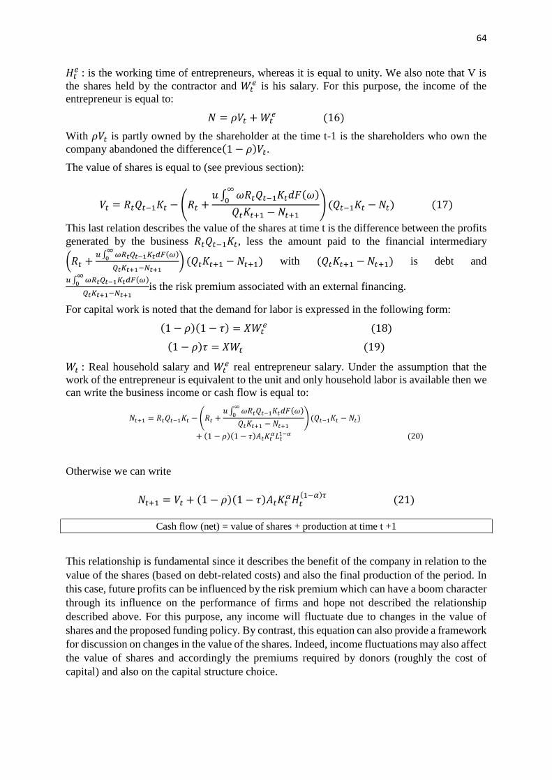
Otherwise we can write

𝑁𝑡+1 = 𝑉𝑡 + (1 − 𝜌)(1 − 𝜏)𝐴𝑡𝐾𝑡𝛼𝐻𝑡

(1−𝛼)𝜏 (21)

Cash flow (net) = value of shares + production at time t +1

This relationship is fundamental since it describes the benefit of the company in relation to the

value of the shares (based on debt-related costs) and also the final production of the period. In

this case, future profits can be influenced by the risk premium which can have a boom character

through its influence on the performance of firms and hope not described the relationship

described above. For this purpose, any income will fluctuate due to changes in the value of

shares and the proposed funding policy. By contrast, this equation can also provide a framework

for discussion on changes in the value of the shares. Indeed, income fluctuations may also affect

the value of shares and accordingly the premiums required by donors (roughly the cost of

capital) and also on the capital structure choice.

65

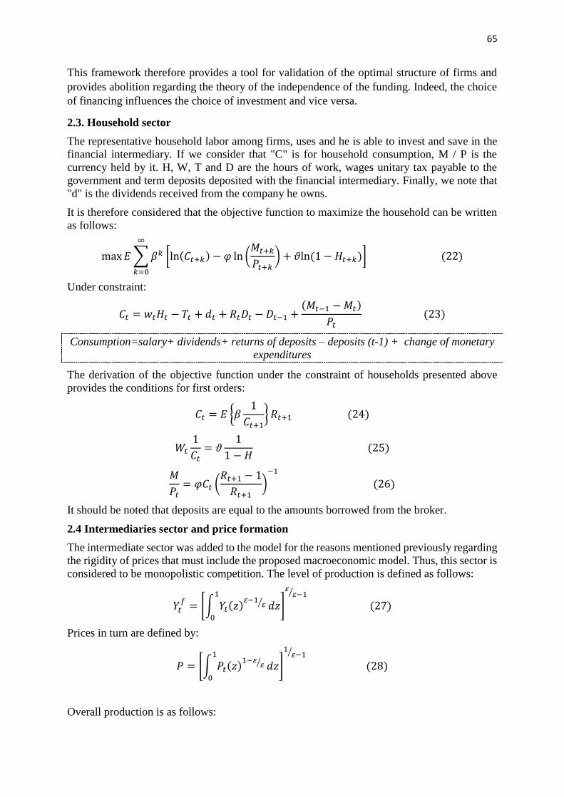
This framework therefore provides a tool for validation of the optimal structure of firms and

provides abolition regarding the theory of the independence of the funding. Indeed, the choice

of financing influences the choice of investment and vice versa.

2.3. Household sector

The representative household labor among firms, uses and he is able to invest and save in the

financial intermediary. If we consider that "C" is for household consumption, M / P is the

currency held by it. H, W, T and D are the hours of work, wages unitary tax payable to the

government and term deposits deposited with the financial intermediary. Finally, we note that

"d" is the dividends received from the company he owns.

It is therefore considered that the objective function to maximize the household can be written

as follows:

max 𝐸 ∑ 𝛽𝑘 [ln(𝐶𝑡+𝑘) − 𝜑 ln (𝑀𝑡+𝑘

𝑃𝑡+𝑘) + 𝜗ln (1 − 𝐻𝑡+𝑘)]

∞

𝑘=0

(22)

Under constraint:

𝐶𝑡 = 𝑤𝑡𝐻𝑡 − 𝑇𝑡 + 𝑑𝑡 + 𝑅𝑡𝐷𝑡 − 𝐷𝑡−1 +(𝑀𝑡−1 − 𝑀𝑡)

𝑃𝑡 (23)

Consumption=salary+ dividends+ returns of deposits – deposits (t-1) + change of monetary

expenditures

The derivation of the objective function under the constraint of households presented above

provides the conditions for first orders:

𝐶𝑡 = 𝐸 {𝛽1

𝐶𝑡+1} 𝑅𝑡+1 (24)

𝑊𝑡

1

𝐶𝑡= 𝜗

1

1 − 𝐻 (25)

𝑀

𝑃𝑡= 𝜑𝐶𝑡 (

𝑅𝑡+1 − 1

𝑅𝑡+1)

−1

(26)

It should be noted that deposits are equal to the amounts borrowed from the broker.

2.4 Intermediaries sector and price formation

The intermediate sector was added to the model for the reasons mentioned previously regarding

the rigidity of prices that must include the proposed macroeconomic model. Thus, this sector is

considered to be monopolistic competition. The level of production is defined as follows:

𝑌𝑡𝑓

= [∫ 𝑌𝑡(𝑧)𝜀−1

𝜀⁄1

0

𝑑𝑧]

𝜀𝜀−1⁄

(27)

Prices in turn are defined by:

𝑃 = [∫ 𝑃𝑡(𝑧)1−𝜀

𝜀⁄1

0

𝑑𝑧]

1𝜀−1⁄

(28)

Overall production is as follows:

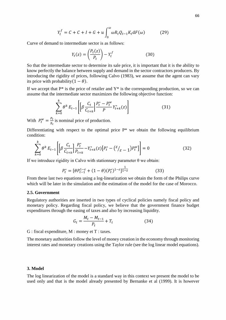
66

𝑌𝑡𝑓

= 𝐶 + 𝐶 + 𝐼 + 𝐺 + 𝑢 ∫ 𝜔𝑅𝑡𝑄𝑡−1𝐾𝑡d𝐹(𝜔)𝜔

0

(29)

Curve of demand to intermediate sector is as follows:

𝑌𝑡(𝑧) = (𝑃𝑡(𝑧)

𝑃𝑡) − 𝑌𝑡

𝑓 (30)

So that the intermediate sector to determine its sale price, it is important that it is the ability to

know perfectly the balance between supply and demand in the sector contractors producers. By

introducing the rigidity of prices, following Calvo (1983), we assume that the agent can vary

its price with probability(1 − 𝜃).

If we accept that P* is the price of retailer and Y* is the corresponding production, so we can

assume that the intermediate sector maximizes the following objective function:

∑ 𝜃𝑘

𝑘

𝑘=0

𝐸𝑡−1 [[𝛽𝐶𝑡

𝐶𝑡+𝑘]

𝑃𝑡∗ − 𝑃𝑡

𝑤

𝑃𝑌𝑡+𝑘

∗ (𝑧)] (31)

With 𝑃𝑡𝑤 =

𝑃𝑡

𝑋𝑡 is nominal price of production.

Differentiating with respect to the optimal price P* we obtain the following equilibrium

condition:

∑ 𝜃𝑘

𝑘

𝑘=0

𝐸𝑡−1 [[𝛽𝐶𝑡

𝐶𝑡+𝑘]

𝑃𝑡∗

𝑃𝑡+𝑘−𝑌𝑡+𝑘

∗ (𝑧)[𝑃𝑡∗ − (휀

휀 − 1⁄ )𝑃𝑡𝑤]] = 0 (32)

If we introduce rigidity in Calvo with stationnary parameter θ we obtain:

𝑃𝑡∗ = [𝜃𝑃𝑡−1

1−𝜀 + (1 − 𝜃)(𝑃𝑡∗)1−𝜀]

11−𝜀 (33)

From these last two equations using a log-linearization we obtain the form of the Philips curve

which will be later in the simulation and the estimation of the model for the case of Morocco.

2.5. Government

Regulatory authorities are inserted in two types of cyclical policies namely fiscal policy and

monetary policy. Regarding fiscal policy, we believe that the government finance budget

expenditures through the easing of taxes and also by increasing liquidity.

𝐺𝑡 =𝑀𝑡 − 𝑀𝑡−1

𝑃𝑡+ 𝑇𝑡 (34)

G : fiscal expenditure, M : money et T : taxes.

The monetary authorities follow the level of money creation in the economy through monitoring

interest rates and monetary creations using the Taylor rule (see the log linear model equations).

3. Model

The log linearization of the model is a standard way in this context we present the model to be

used only and that is the model already presented by Bernanke et al (1999). It is however

67

important to note that the equations of the models have the particularity to resume financial

accelerator presented in the previous section.

If we want to summarize the characteristics of the model, it was noted that:

• It is composed of three central agents (households, entrepreneurs and intermediaries)

with the presence of monetary and fiscal authorities;

• it takes into account the rigidity of prices Calvo (1983) by incorporating imperfect

competition in the intermediate sector and the ability to set prices according to a given

probability between 0 and 1 to describe price inertia;

• Contractors are pure and perfect competition to allow the formation of an optimal

financial contract;

• Entrepreneurs can borrow from financial intermediaries to occur during a period;

• The intermediary requires a risk premium that determines the level of cost of capital and

the impact of investment choices.

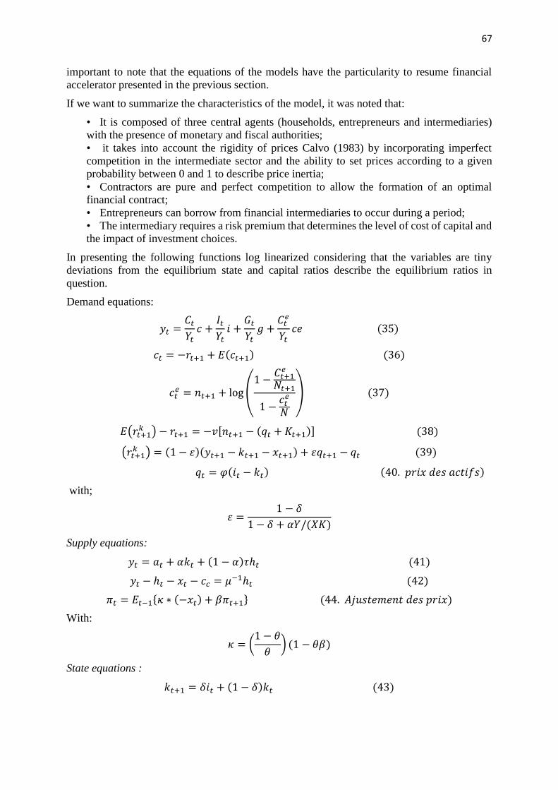
In presenting the following functions log linearized considering that the variables are tiny

deviations from the equilibrium state and capital ratios describe the equilibrium ratios in

question.

Demand equations:

𝑦𝑡 =𝐶𝑡

𝑌𝑡𝑐 +

𝐼𝑡

𝑌𝑡𝑖 +

𝐺𝑡

𝑌𝑡𝑔 +

𝐶𝑡𝑒

𝑌𝑡𝑐𝑒 (35)

𝑐𝑡 = −𝑟𝑡+1 + 𝐸(𝑐𝑡+1) (36)

𝑐𝑡𝑒 = 𝑛𝑡+1 + log (

1 −𝐶𝑡+1

𝑒

𝑁𝑡+1

1 −𝑐𝑡

𝑒

𝑁

) (37)

𝐸(𝑟𝑡+1𝑘 ) − 𝑟𝑡+1 = −𝑣[𝑛𝑡+1 − (𝑞𝑡 + 𝐾𝑡+1)] (38)

(𝑟𝑡+1𝑘 ) = (1 − 휀)(𝑦𝑡+1 − 𝑘𝑡+1 − 𝑥𝑡+1) + 휀𝑞𝑡+1 − 𝑞𝑡 (39)

𝑞𝑡 = 𝜑(𝑖𝑡 − 𝑘𝑡) (40. 𝑝𝑟𝑖𝑥 𝑑𝑒𝑠 𝑎𝑐𝑡𝑖𝑓𝑠)

with;

휀 =1 − 𝛿

1 − 𝛿 + 𝛼𝑌/(𝑋𝐾)

Supply equations:

𝑦𝑡 = 𝑎𝑡 + 𝛼𝑘𝑡 + (1 − 𝛼)𝜏ℎ𝑡 (41)

𝑦𝑡 − ℎ𝑡 − 𝑥𝑡 − 𝑐𝑐 = 𝜇−1ℎ𝑡 (42)

𝜋𝑡 = 𝐸𝑡−1{𝜅 ∗ (−𝑥𝑡) + 𝛽𝜋𝑡+1} (44. 𝐴𝑗𝑢𝑠𝑡𝑒𝑚𝑒𝑛𝑡 𝑑𝑒𝑠 𝑝𝑟𝑖𝑥)

With:

𝜅 = (1 − 𝜃

𝜃) (1 − 𝜃𝛽)

State equations :

𝑘𝑡+1 = 𝛿𝑖𝑡 + (1 − 𝛿)𝑘𝑡 (43)

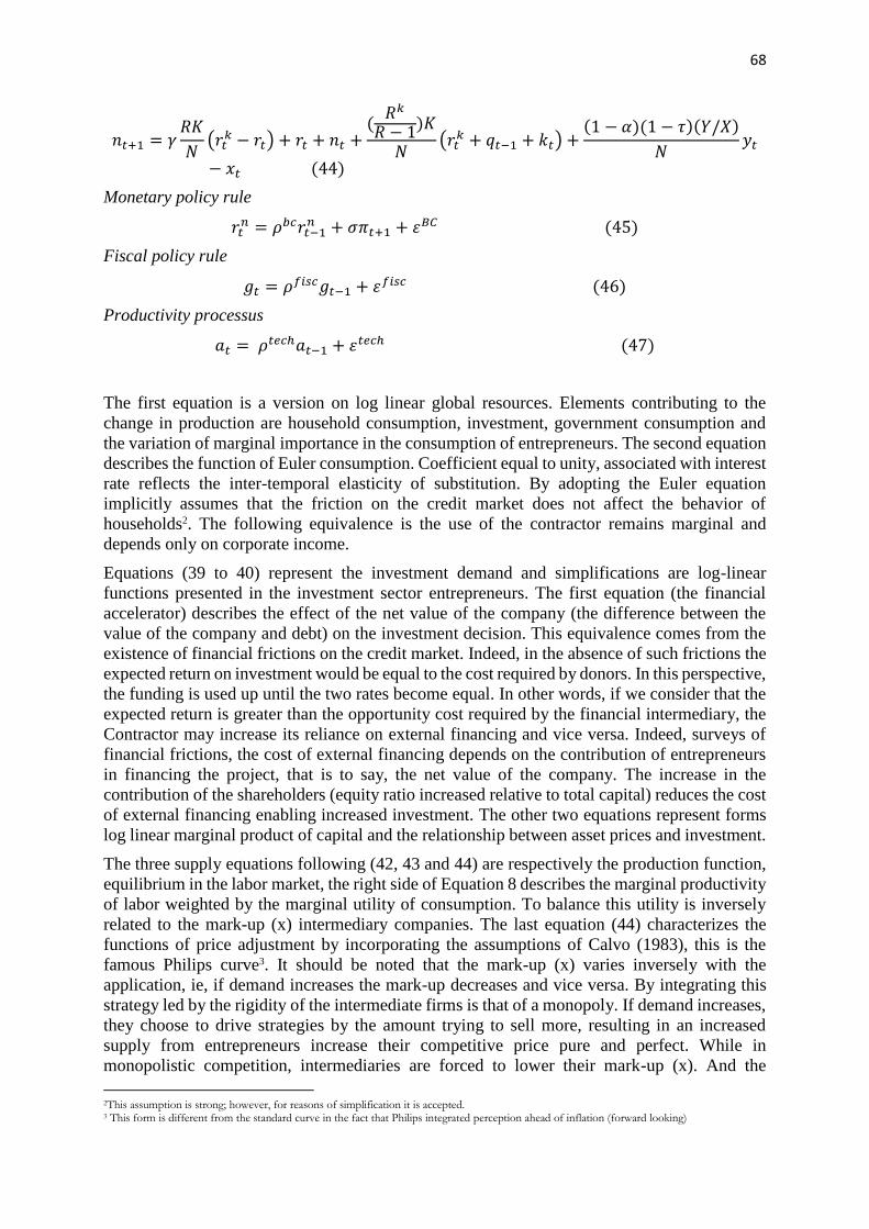
68

𝑛𝑡+1 = 𝛾𝑅𝐾

𝑁(𝑟𝑡

𝑘 − 𝑟𝑡) + 𝑟𝑡 + 𝑛𝑡 +(

𝑅𝑘

𝑅 − 1)𝐾

𝑁(𝑟𝑡

𝑘 + 𝑞𝑡−1 + 𝑘𝑡) +(1 − 𝛼)(1 − 𝜏)(𝑌/𝑋)

𝑁𝑦𝑡

− 𝑥𝑡 (44)

Monetary policy rule

𝑟𝑡𝑛 = 𝜌𝑏𝑐𝑟𝑡−1

𝑛 + 𝜎𝜋𝑡+1 + 휀𝐵𝐶 (45)

Fiscal policy rule

𝑔𝑡 = 𝜌𝑓𝑖𝑠𝑐𝑔𝑡−1 + 휀𝑓𝑖𝑠𝑐 (46)

Productivity processus

𝑎𝑡 = 𝜌𝑡𝑒𝑐ℎ𝑎𝑡−1 + 휀𝑡𝑒𝑐ℎ (47)

The first equation is a version on log linear global resources. Elements contributing to the

change in production are household consumption, investment, government consumption and

the variation of marginal importance in the consumption of entrepreneurs. The second equation

describes the function of Euler consumption. Coefficient equal to unity, associated with interest

rate reflects the inter-temporal elasticity of substitution. By adopting the Euler equation

implicitly assumes that the friction on the credit market does not affect the behavior of

households2. The following equivalence is the use of the contractor remains marginal and

depends only on corporate income.

Equations (39 to 40) represent the investment demand and simplifications are log-linear

functions presented in the investment sector entrepreneurs. The first equation (the financial

accelerator) describes the effect of the net value of the company (the difference between the

value of the company and debt) on the investment decision. This equivalence comes from the

existence of financial frictions on the credit market. Indeed, in the absence of such frictions the

expected return on investment would be equal to the cost required by donors. In this perspective,

the funding is used up until the two rates become equal. In other words, if we consider that the

expected return is greater than the opportunity cost required by the financial intermediary, the

Contractor may increase its reliance on external financing and vice versa. Indeed, surveys of

financial frictions, the cost of external financing depends on the contribution of entrepreneurs

in financing the project, that is to say, the net value of the company. The increase in the

contribution of the shareholders (equity ratio increased relative to total capital) reduces the cost

of external financing enabling increased investment. The other two equations represent forms

log linear marginal product of capital and the relationship between asset prices and investment.

The three supply equations following (42, 43 and 44) are respectively the production function,

equilibrium in the labor market, the right side of Equation 8 describes the marginal productivity

of labor weighted by the marginal utility of consumption. To balance this utility is inversely

related to the mark-up (x) intermediary companies. The last equation (44) characterizes the

functions of price adjustment by incorporating the assumptions of Calvo (1983), this is the

famous Philips curve3. It should be noted that the mark-up (x) varies inversely with the

application, ie, if demand increases the mark-up decreases and vice versa. By integrating this

strategy led by the rigidity of the intermediate firms is that of a monopoly. If demand increases,

they choose to drive strategies by the amount trying to sell more, resulting in an increased

supply from entrepreneurs increase their competitive price pure and perfect. While in

monopolistic competition, intermediaries are forced to lower their mark-up (x). And the

2This assumption is strong; however, for reasons of simplification it is accepted. 3 This form is different from the standard curve in the fact that Philips integrated perception ahead of inflation (forward looking)

69

negative sign in the relationship of Philips captures the dynamics under the assumption of price

rigidity. In this perspective, inflation depends on price rigidity and the coefficient κ is inversely

related to the stiffness coefficient θ.

The following two equations (44 and 45) are a representation of the state variables; shareholders

and net income in a respective manner. The evolution of net income (equation 45) depends on

the profitability of entrepreneurs (RK) from the capital (N) and also the delay of the net income

of the previous period. It should be noted that the difference between the rate of return on capital

and the risk-free rate has a disproportionate impact on the net because of the existence of the

financial accelerator presented earlier. In this sense, this difference is weighted by the ratio

between capital and contribution of entrepreneurs (K/N). In practice, the financial accelerator

mechanism is given via the net income of the firm affects investment choices via equation (39)

arbitration. In addition, a surplus of this model is the ability to characterize the evolution of the

net income of the firm.

The last block of equations describes the reaction functions of the monetary and fiscal

authorities. The central bank reacted with a rule governing interest rates with the instrument

nominal interest rate. Although the monetary policy life standard to reduce fluctuations in

inflation following the changes in the output gap, the use of interest rate can be useful also to

reduce the fluctuations from the financial accelerator presented in this model. The last two

equations (47 and 48) relate to the fiscal rule and the process generating productivity shocks.

These processes were considered to have autoregressive behavior.

4. Integrate Speculative Bubbles to Macroeconomic Model

The model presented above is a financial accelerator model that captures financial frictions in

the credit market. The integration of decision theories helped form a financial contract that

supports external financing of investments. However, the integration of financial intermediation

is overwhelming problems related to price formation in financial markets. The financial system

is often confronted with problems of disconnection prices fundamental values due to the

existence of high probability of resale rights of shareholders. These deviations of asset prices

give birth to what is called speculative bubbles.

We presented in the previous sections that the price of capital is equal to:

𝑄𝑡 =1

[𝜃′ (𝐼𝑡

𝐾𝑡)]

(48)

It is assumed that the fundamental price is 𝑄𝑡 which is determined from the future growth

prospects and dividends earned by the owners of capital.

𝑄𝑡 =𝐷𝑡+1 + (1 − 𝛿)𝑄𝑡+1

𝑅𝑡+1𝑞 (49)

This relationship describes the fundamental value of a single period. It should be noted that δ

is the depreciation of the capital D is dividends.

To take account of speculative bubbles, we consider the hypothesis that asset prices may deviate

from fundamental prices. Note that S is the real price, so we adopt the presentation of Blanchard

et al (1988) we can write:

𝑎(𝑆𝑡 − 𝑄𝑡) = 𝜕𝐵𝑡+1 (50)

70

With 𝜕 actualization factor and a<1. Without bubbles 𝜕 = 0. According to the definition of the

bubble we can write the rate of return based on the actual price of profitability related to

fundamental price.

𝑅𝑡+1𝑠 = 𝑅𝑡+1

𝑞 [𝑎(1 − 𝛿) + (1 − 𝑎(1 − 𝛿))𝑄𝑡

𝑆𝑡] (51)

According to this relationship, in the absence of bubbles Q=S is then 𝑅𝑡+1𝑠 = 𝑅𝑡+1

𝑞.

Taking into account the existence of bubble in the capital market, public authorities must take

into account this reality by integrating it into their decision device in order to avoid the adverse

effects of bubbles. In this sense Bernanke et al (1999) proposes to increase the rule of the central

bank through the introduction of changes in asset prices. So the new rule would be:

𝑟𝑡𝑛 = 𝜌𝑏𝑐𝑟𝑡−1

𝑛 + 𝜎𝜋𝑡+1 + 𝜎𝑏𝑢𝑏𝑏𝑙𝑒𝑠 log (𝑆

𝑆𝑡−1) (52)

The interest rate adjustment is done by taking into account the movements of inflation and also

the evolution of asset prices. In other words, the central bank reacted in response to the prospect

of inflation and also when asset prices begin to show a significant increase.

5. Estimate Model

The model with financial frictions on the credit market can include credit dynamics in an

environment that may be affected by informational asymmetries. And also in the presence of

asset price model can also incorporate the possibility of existence of a rational nature bubble.

The model is used to estimate mode using the Bayesian approach. Dynare clone was used for

this purpose. The Moroccan data were used to determine the set of parameters with which the

model will be calibrated.

The data used for calibration are extracted from the HCP. However, it should be noted that most

of the variables are expressed in deviation from the logarithm of the equilibrium state.

We use the following relation for all data, except for the case of ratios that make up the model:

�̌� =𝑥𝑡

𝑥∗− 1 𝑒𝑡 𝑥𝑡 = (�̌� + 1)𝑥∗ (53)

𝑥∗is potential value. To arrive at this estimate variable we use the HP filter that determines the

long-term trend. This relationship is used later in the result set. It should be noted that the

impulse responses are expressed in deviation from the steady state (Table 1).

The parameters used and the initial values of some ratios were calibrated according to the

values shown in the table 2.

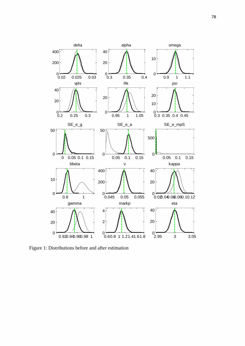
The estimation method used is the Bayesian method on the clone Dynare using MCMC

algorithms to achieve the parameters which determine the distributions were calibrated.

Estimates were performed on data from 2000 to 2011 on a quarterly basis. The estimation

results of the model are shown in the table below in comparison with baseline values selected

for the Moroccan economy. It should be noted that two types of models will be compared with

a subsequent possibility of the presence of bubbles and the second representing a fundamental

equilibrium.

The estimated DSGE model with frictions on the credit market in the case of Morocco confirms

an important finding in relation to the propagation of macroeconomic shocks.

71

The assumptions made in the theoretical development of the model, including the ability of

firms to use financial intermediaries, can provide a framework for analyzing macroeconomic

conditions in Morocco taking into account the frictions that can impede the relationship

between the system financial intermediation and investment. Indeed, the impulse responses

using three types of shocks, monetary, fiscal and productivity argue that the existence of the

risk premium (after agency costs imposed by financial intermediaries) are likely to impact the

decisions investment firms.

5.1. Financial frictions in Morocco

In addition to the results obtained by comparing a model without frictions financial, where the

rate of return expected by investors is equal to the risk-free rate (absence of agency costs), with

a financial accelerator model confirms that the integration of friction costs and additional

funding from external amplify macroeconomic shocks.

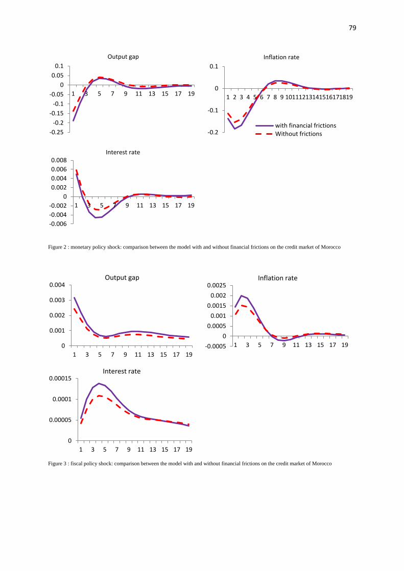
The introduction of frictions in the model confirmed that macroeconomic shocks tend to grow

on the basis of the existence of risk premium related to the use of external financing. The

monetary policy shock confirms that the response of the output gap is more or less important

when integrated frictions in the credit market, it is the same with regard to interest rates and

inflation. Regarding the fiscal shock results seem to produce the same trends. On the basis of

these two graphs it is clear that the financial accelerator process is crucial in the dynamic

propagation of shocks. Indeed, each decision using cyclical monetary and fiscal instruments

will tend to be amplified as a result of existence of frictions on the credit market.

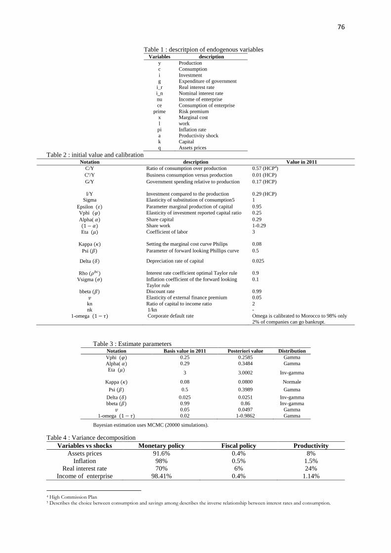
This is also confirmed by analyzing the variance decomposition model which shows that the

impact of monetary and fiscal policy have a significant impact on the variables that drive much

of the investment decision. As a side note, therefore, that rising interest rates explain much of

the variation in the prices of assets and net income of firms (flow). In this sense, decisions on

monetary and fiscal control may with huge effects on the choice of financing and investment.

Furthermore the ability of the model to take into account the phenomenon of financial

accelerator is capable of producing results taking into account the risk premium. Thus, the

model allows reproducing information on the evolution of risks to businesses and default rates

may overwhelm when significant decrease rates of return beyond the rate charged by financial

intermediaries.

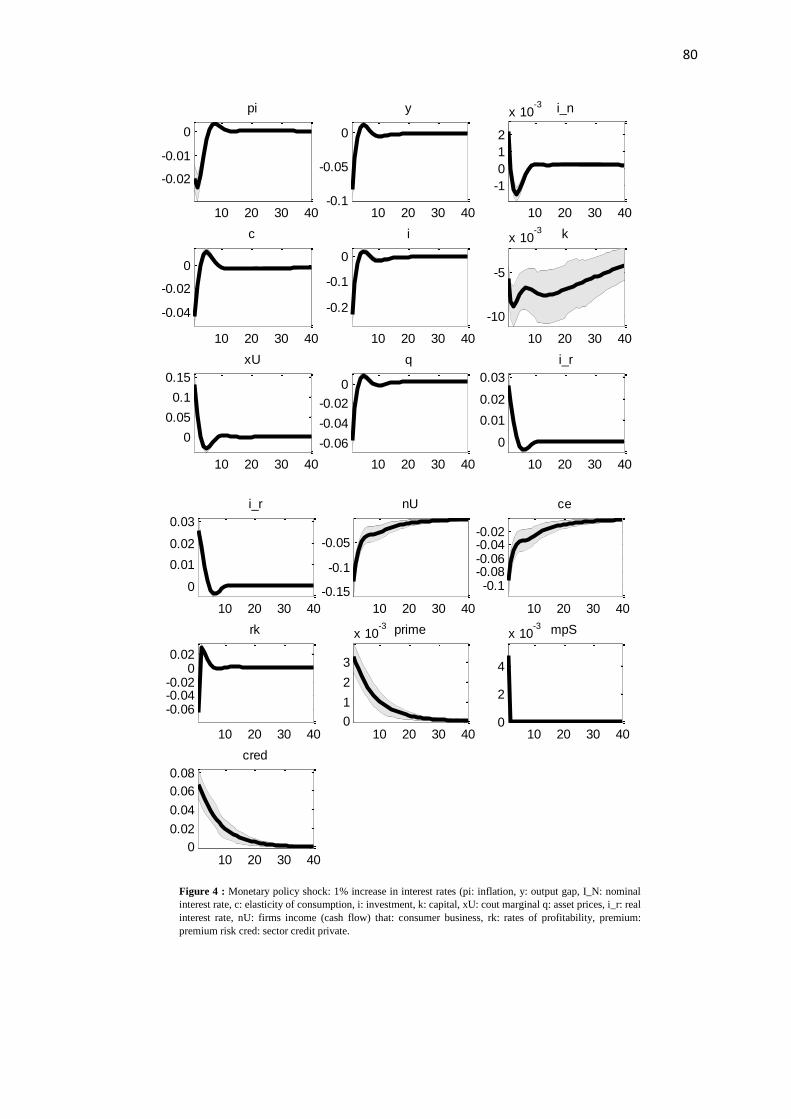
To describe the relevance of this model in terms of analysis, we use the impulse responses of

the estimated model. The analysis of impulse responses is limited solely to monetary policy

shock due to a 1% increase in interest rates.

The effects of a 1% increase in interest rates on all macroeconomic aggregates are more or less

intuitive and can confirm the relevance of the model with financial frictions. The most

important is that this shock also impact financial aggregates which attract investment decision

in Morocco. In fact, higher interest rates reflected positively on the risk premium by increasing

requirements of banks in terms of opportunity cost, which negatively affects the profitability of

investments and the income generated by firms. Also, this impact occurs by lowering the price

of assets that are negatively correlated with interest rates, however, we can see that the use of

financial intermediaries increases justified by lower revenue firms. On a theoretical level, the

decline in cash flow encourages firms to have a heavy reliance on banks and an increase of

conflicts of interest and premiums accordingly.

Furthermore, the analysis can produce this type of model including this informational

asymmetry on the credit market, the model taking into account the financial accelerator helps

explain some episodes experienced by the Morocco in recent years.

72

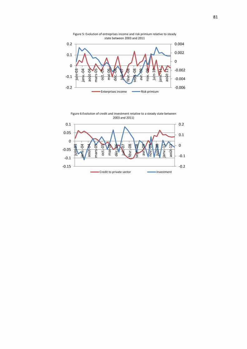
Growth experienced by Morocco during the last decade and specifically between 2005 and

2010, this is manifested by an increase in overall economic aggregates and in particular the

income generated by firms and production that follows. This increase in production and income

was primarily due to lower risk premiums on the credit market. In fact the opening on external

financing and lower interest rates resulted in a better appreciation of the value of the productive

sector. However from 2010, the revenues of firms experienced a downward trend and risk

premiums have recorded significant increases.

In the same vein, we note that during the years 2003 to 2008, investment firms increased

significantly, although the use of external finance remains low. From 2009 we see that the

investment starts fell thus describing a drop in flow due to lower revenues. This justifies the

use of more external financing during this period justifying and tighter financing conditions in

Morocco due to higher risk premiums.

5.2. Speculative bubbles and central bank rule

The existence of asset prices in the macroeconomic framework facilitates the integration of the

notion of a speculative bubble, in relation to which the monetary authorities should be

responsive on adjusting the interest rate to extreme fluctuations in asset prices in markets

capital. To this end, the Central Bank should include asset prices in monetary policy by

interacting according to deviations of price and in case of formation of speculative bubbles.

In this section we prove that the use of a monetary rule taking into account asset prices ensures

better stability of the macroeconomic framework. To this end, we compare two types of

monetary rule namely the conventional Taylor rule and a second incorporating asset prices.

This counterfactual analysis to choose the most optimal rule in favor of better regulation of the

macroeconomic framework. In addition, the integration of asset prices in the device allows to

take into account the financial stability to regulate the price deviations from the fundamental

value. In fact, most of dysfunctional capital markets have reasons for the formation of bubbles

that never ceases to produce rational expectations wrong.

In this sense, the innovation of this work is to propose to the use of a monetary rule including

responsiveness to future changes in asset prices. And two rules have competition:

A rule increased asset price (S):

𝑟𝑡𝑛 = 𝜌𝑏𝑐𝑟𝑡−1

𝑛 + 𝜎𝜋𝑡+1 + 𝜎𝑏𝑢𝑏𝑏𝑙𝑒𝑠log (𝑆

𝑆𝑡−1)

The forward looking Taylor rule:

𝑟𝑡𝑛 = 𝜌𝑏𝑐𝑟𝑡−1

𝑛 + 𝜎𝜋𝑡+1

The counterfactual analysis we use is based on the study of standard deviation of key variables

that are used to verify the stability of the macroeconomic framework. The results we obtained

are transcribed in the table below:

The analysis of the volatility of macroeconomic aggregates indicates that the presence of

bubbles in asset prices, it is more appropriate to use a monetary rule including changes in asset

prices. In this sense, the central bank should react each time by conventional instrument to

achieve the reduction of macroeconomic instability after a slide in prices of their underlying

trend. The volatility of macroeconomic aggregates is lower when using a Taylor rule augmented

by asset prices. The standards deviations in Table 3 describes a low volatility when the

monetary authorities use a rule taking into account changes in asset prices.

73

6. Conclusion

Using the model with frictions in the credit market has confirmed that macroeconomic shocks

tend to grow due to the existence of a phenomenon from the accelerator agency costs required

by financial intermediaries. The framework of macroeconomic analysis that must now provide

the monetary authority to stabilize the economy must include the credit market to ensure better

conduct of monetary policy. Regarding financial stability, expanding the model to take into

account the bubbles will better macro-prudential regulation as a result of taking into account

the volatility of asset prices. In this sense, the monetary rule should be rehabilitated to include

a new component, namely asset prices.

Endnotes

Dr. Firano Zakaria, Faculty of laws, economics and socials sciences Rabat-Agdal. Email:

firanou@yahoo.fr.

74

References

Bernanke, B., Gertler, M., 1989. Agency costs, net worth and business fluctuations. American

Economic Review 79, 14–31.

Bernanke, B., Gertler, M., 2000, Monetary policy and asset price volatility. Working paper No.

7559. NBER.

Bernanke, B., Gertler, M., Gilchrist, S., 1999. The financial accelerator in a quantitative

business cycle framework. In: Handbook of Macroeco-nomics. North-Holland, Amsterdam.

Blanchard, O.J., Kahn, C.M., 1980. The solution of linear difference models under rational

expectations. Econometrica 48, 1305–1311.

Bouakez, H., Cardia, E., Ruge-Murcia, F., 2005. Habit formation and the persistence of

monetary policy shocks. Journal of Monetary Economics 52, 1073–1088.

Calvo, G.A., 1983. Staggered prices in a utility-maximizing framework. Journal of Monetary

Economics 12, 383–398.

Carlstrom, G., Fuerst, T.S., 1997. Agency costs, net worth, business fluctuations: A computable

general equilibrium analysis. American Economic Review 87, 893–910.

Cespedes, L.F., Chang, R., Velasco, A., 2004. Balance sheets and exchange rate policy.

American Economic Review 94, 1183–1193.

Christiano, L., Eichenbaum, M., Evans, C., 2005. Nominal rigidities and the dynamic effects

of a shock to monetary policy. Journal of Political Economy 113, 1–45.

Christiano, L.J., Motto, R., Rostagno, M., 2003. The Great Depression and the Friedman–

Schwartz hypothesis. Journal of Money, Credit, Bank-ing 35, 1119–1197.

Cook, D., 1999. The liquidity effect and money demand. Journal of Monetary Economics 43,

377–390.

Dib, A., 2003. An estimated Canadian DSGE model with nominal and real rigidities. Canadian

Journal of Economics 36, 949–972.

Dib, A., 2006. Nominal rigidities and monetary policy in Canada. Journal of Macroeconomics

28, 285–304.

Elekdag, S., Justiniano, A., Tchakarov, I., 2006. An estimated small open economy model of

the financial accelerator. IMF Staff Papers 53, 219–241.

Fisher I., 1932, The Debt Deflation Theory Of Great Depressions , Econometrica, 1 : 337-57.

Fukunaga, I., 2002. Financial accelerator effects in Japan’s business cycles. Working paper No.

2002, Bank of Japan.

Gertler, M., Gilchrist, S., Natalucci, F., 2003. External constraints on monetary policy and the

financial accelerator. Working paper No. 139. BIS (Journal of Money, Credit, Banking, in

press).

Gilchrist, S., 2004. Financial markets and financial leverage in a two-country world economy.

In: Banking Market Structure and Monetary Policy. Central Bank of Chile, Santiago.

Greenwood, J., Hercowitz, Z., Huffman, G., 1988. Investment, capacity utilization, the real

business cycle. American Economic Review 78, 402–417.

Greenwood, J., Hercowitz, Z., Krusell, P., 2000. The role of investment-specific technological

change in the business cycle. European Economic Review 44, 91–115.

Hall, S., 2001. Financial accelerator effects in UK business cycles. Working paper No. 150.

Bank of England.

Hamilton, J.D., 1994. Time Series Analysis. Princeton Univ. Press, Princeton.

Iacoviello, M., 2005. House prices, borrowing constraints and monetary policy in the business

cycle. American Economic Review 95, 739–764.

Ian Christensen, Ali Dib, 2007, The financial accelerator in an estimated New Keynesian

model, Review of Economic Dynamics 11 (2008) 155–178

Ireland, P.N., 2003. Endogenous money or sticky prices? Journal of Monetary Economics 50,

1623–1648.

75

Kiyotaki N. And J. Moore, 2007, Credit Cycles ., Journal Of Political Economy, 105, Pp.

211248.

Kiyotaki, N., Moore, J., 1997. Credit cycles. The Journal of Political Economy 105, 211–248.

Meier, A., Müller, G.J., 2006. Fleshing out the monetary transmission mechanism: output

composition and the role of financial frictions. Journal of Money, Credit, Banking 38, 1999–

2133.

Minsky H. P. 1977, A Theory Of Systemic Fragility, In E. I. Altman And A. W. Sametz (Eds.),

Financial Crises, Wiley, New York.

Mishkin F. S. 1991, Asymmetric Information And Financial Crises: A Historical Perspective,

Financial Markets And Financial Crises, Hubbard R G (Ed), University Of Chicago Press,

Chicago.

Primiceri, G.E., 2006. The time varying volatility of macroeconomic fluctuations, Working

paper No. 12022. NBER.

Taylor, J.B., 1993. Discretion versus policy rules in practice. Carnegie-Rochester Conference

Series on Public Policy 39, 195–214.

Tovar C., 2006. Devaluations, output, the balance sheet effect: A structural econometric

analysis. Working Paper No. 215. Bank for International Settlements.

Yun, T., 1996. Nominal price rigidity, money supply endogeneity, business cycles. Journal of

Monetary Economics 37, 345–370.

76

Table 1 : descritpion of endogenous variables Variables description

y Production

c Consumption

i Investment g Expenditure of government

i_r Real interest rate

i_n Nominal interest rate nu Income of enterprise

ce Consumption of enterprise

prime Risk premium x Marginal cost

l work

pi Inflation rate a Productivity shock

k Capital

q Assets prices

Table 2 : initial value and calibration Notation description Value in 2011

C/Y Ratio of consumption over production 0.57 (HCP4)

Ce/Y Business consumption versus production 0.01 (HCP)

G/Y Government spending relative to production

0.17 (HCP)

I/Y Investment compared to the production 0.29 (HCP) Sigma Elasticity of substitution of consumption5 1

Epsilon (휀) Parameter marginal production of capital 0.95

Vphi (𝜑) Elasticity of investment reported capital ratio 0.25

Alpha( 𝛼) Share capital 0.29

(1 − 𝛼) Share work 1-0.29

Eta (𝜇)

Coefficient of labor 3

Kappa (𝜅) Setting the marginal cost curve Philips 0.08

Psi (𝛽) Parameter of forward looking Phillips curve 0.5

Delta (𝛿) Depreciation rate of capital

0.025

Rho (𝜌𝑏𝑐) Interest rate coefficient optimal Taylor rule 0.9

Vsigma (𝜎) Inflation coefficient of the forward looking

Taylor rule

0.1

bbeta (𝛽) Discount rate 0.99

𝑣 Elasticity of external finance premium 0.05

kn Ratio of capital to income ratio 2

nk 1/kn -

1-omega (1 − 𝜏) Corporate default rate Omega is calibrated to Morocco to 98% only

2% of companies can go bankrupt.

Table 3 : Estimate parameters Notation Basis value in 2011 Posteriori value Distribution

Vphi (𝜑) 0.25 0.2585 Gamma

Alpha( 𝛼) 0.29 0.3484 Gamma

Eta (𝜇)

3 3.0002 Inv-gamma

Kappa (𝜅) 0.08 0.0800 Normale

Psi (𝛽) 0.5 0.3989 Gamma

Delta (𝛿) 0.025 0.0251 Inv-gamma

bbeta (𝛽) 0.99 0.86 Inv-gamma

𝑣 0.05 0.0497 Gamma

1-omega (1 − 𝜏) 0.02 1-0.9862 Gamma

Bayesian estimation uses MCMC (20000 simulations).

Table 4 : Variance decomposition

Variables vs shocks Monetary policy Fiscal policy Productivity

Assets prices 91.6% 0.4% 8%

Inflation 98% 0.5% 1.5%

Real interest rate 70% 6% 24%

Income of enterprise 98.41% 0.4% 1.14%

4 High Commission Plan 5 Describes the choice between consumption and savings among describes the inverse relationship between interest rates and consumption.

77

Table 1 : counterfactual analysis

Rules Std Taylor rule with assets

prices

Std Taylor rule without assets

prices

Output gap 1.0427 0.5121

Inflation 0.0216 0.0265

Real interest rate 0.0201 0.0172

Risk premium 0.0717 0.0333

Investment 0.5356 0.4176

78

Figure 1: Distributions before and after estimation

0.02 0.025 0.030

200

400

delta

0.3 0.35 0.40

20

40

alpha

0.9 1 1.10

10

omega

0.2 0.25 0.30

20

40

vphi

0.95 1 1.050

20

Rk

0.3 0.35 0.4 0.450

10

20

psi

0 0.05 0.1 0.150

50

SE_e_g

0.05 0.1 0.150

50

SE_e_a

0.05 0.1 0.150

500

SE_e_mpS

0.8 10

10

bbeta

0.045 0.05 0.0550

200

400

v

0.020.040.060.080.10.120

20

40

kappa

0.920.940.960.98 10

20

40

gamma

0.60.8 1 1.21.41.61.80

2

4

markp

2.95 3 3.050

20

40

eta

79

Figure 2 : monetary policy shock: comparison between the model with and without financial frictions on the credit market of Morocco

Figure 3 : fiscal policy shock: comparison between the model with and without financial frictions on the credit market of Morocco

-0.25

-0.2

-0.15

-0.1

-0.05

0

0.05

0.1

1 3 5 7 9 11 13 15 17 19

Output gap

-0.2

-0.1

0

0.1

1 2 3 4 5 6 7 8 9 10111213141516171819

Inflation rate

with financial frictionsWithout frictions

-0.006

-0.004

-0.002

0

0.002

0.004

0.006

0.008

1 3 5 7 9 11 13 15 17 19

Interest rate

0

0.001

0.002

0.003

0.004

1 3 5 7 9 11 13 15 17 19

Output gap

-0.0005

0

0.0005

0.001

0.0015

0.002

0.0025

1 3 5 7 9 11 13 15 17 19

Inflation rate

0

0.00005

0.0001

0.00015

1 3 5 7 9 11 13 15 17 19

Interest rate

80

Figure 4 : Monetary policy shock: 1% increase in interest rates (pi: inflation, y: output gap, I_N: nominal

interest rate, c: elasticity of consumption, i: investment, k: capital, xU: cout marginal q: asset prices, i_r: real

interest rate, nU: firms income (cash flow) that: consumer business, rk: rates of profitability, premium:

premium risk cred: sector credit private.

10 20 30 40

-0.02

-0.01

0

pi

10 20 30 40-0.1

-0.05

0

y

10 20 30 40

-1

0

1

2

x 10-3 i_n

10 20 30 40

-0.04

-0.02

0

c

10 20 30 40

-0.2

-0.1

0

i

10 20 30 40

-10

-5

x 10-3 k

10 20 30 40

0

0.05

0.1

0.15

xU

10 20 30 40

-0.06

-0.04

-0.02

0

q

10 20 30 40

0

0.01

0.02

0.03

i_r

10 20 30 40

0

0.01

0.02

0.03

i_r

10 20 30 40

-0.15

-0.1

-0.05

nU

10 20 30 40

-0.1-0.08-0.06-0.04-0.02

ce

10 20 30 40

-0.06-0.04-0.02

00.02

rk

10 20 30 400

1

2

3

x 10-3 prime

10 20 30 400

2

4

x 10-3 mpS

10 20 30 400

0.02

0.04

0.06

0.08

cred

81

-0.006

-0.004

-0.002

0

0.002

0.004

-0.2

-0.1

0

0.1

0.2

juin

-03

jan

v.-0

4

aoû

t-0

4

mar

s-0

5

oct

.-0

5

mai

-06

déc

.-0

6

juil.

-07

févr

.-0

8

sep

t.-0

8

avr.

-09

no

v.-0

9

juin

-10

jan

v.-1

1

aoû

t-1

1

Figure 5: Evolution of entreprises income and risk primium relative to steady state between 2003 and 2011

Enterprises income Risk primium

-0.2

-0.1

0

0.1

0.2

-0.15

-0.1

-0.05

0

0.05

0.1

juin

-03

jan

v.-0

4

aoû

t-0

4

mar

s-0

5

oct

.-0

5

mai

-06

déc

.-0

6

juil.

-07

févr

.-0

8

sep

t.-0

8

avr.

-09

no

v.-0

9

juin

-10

jan

v.-1

1

aoû

t-1

1

Figure 6:Evolution of credit and investment retative to a steady state between 2003 and 2011)

Credit to private sector Investment