Embed Size (px)
Citation preview
University of Arkansas, FayettevilleScholarWorks@UARK
Theses and Dissertations
12-2012
Essays in Development Economics and Economicsof the FamilyAaron JohnsonUniversity of Arkansas, Fayetteville
Follow this and additional works at: http://scholarworks.uark.edu/etd
Part of the Finance Commons, and the Growth and Development Commons
This Dissertation is brought to you for free and open access by ScholarWorks@UARK. It has been accepted for inclusion in Theses and Dissertations byan authorized administrator of ScholarWorks@UARK. For more information, please contact [email protected], [email protected].
Recommended CitationJohnson, Aaron, "Essays in Development Economics and Economics of the Family" (2012). Theses and Dissertations. 570.http://scholarworks.uark.edu/etd/570
ESSAYS IN DEVELOPMENT ECONOMICS
AND ECONOMICS OF THE FAMILY
ESSAYS IN DEVELOPMENT ECONOMICS
AND ECONOMICS OF THE FAMILY
A dissertation submitted in partial fulfillment
of the requirements for the degree of
Doctor of Philosophy in Economics
By
Aaron Lee Johnson
University of Nebraska
Bachelor of Arts in Business Administration, 2002
University of Arkansas
Master of Arts in Economics, 2009
December 2012
University of Arkansas
ABSTRACT
Chapter 1 explores a potential solution to the continuing disequlibrium in microfinance markets.
I design a mechanism to aid in securitization of microloans, using a dynamic investment pool
governed by a Central Microcredit Clearinghouse (CMC), that would sell investment units back
to MFIs and outside investors simultaneously. The CMC would serve as a catalyst to this other
avenue of microcredit financing, securitization of microloans, which could help spawn the type
of growth in investor-based funding of MFIs that is so urgently needed. Chapter 2 analyzes
Official Development Assistance (ODA) commitment and disbursement activity in terms of
motivation, considering that the difference between bilateral aid commitments and disbursements
may be related to the business cycle of the donor country. The annual disbursement gap is
calculated for each pair for each year, as well as a cumulative disbursement gap, and these are
regressed against multiple cyclicality measures of income and a set of control variables. It is
found in multiple specifications that the cumulative disbursement gap is generally procyclical,
much as aid itself, although the cyclicality of aid depends on the cyclicality measure. This is
confirmed with four extensions designed mainly as robustness checks. Chapter 3 uses both the
round six and 2006-2008 National Survey of Family Growth (NSFG) data for both male and
female respondents along with macroeconomic data over the same time period to test a number
of theoretical questions regarding changes in relationship exit costs and their effects on behavior
in cohabitation, marriage, and separation. I find that our proxy for cohabitation surplus and exit
costs significantly affects subsequent decisions of cohabitation, marriage, separation, and
divorce. Also, marriage hazard rates are related to these changing exit costs in ways consistent
with recent advances in theory.
This dissertation is approved for recommendation
to the Graduate Council
Dissertation Director:
_______________________________________
Dr. Andrew W. Horowitz
Dissertation Committee:
_______________________________________
Dr. Amy Farmer
_______________________________________
Dr. Raja Kali
DISSERTATION DUPLICATION RELEASE
I hereby authorize the University of Arkansas Libraries to duplicate this dissertation when
needed for research and/or scholarship.
Agreed __________________________________________
Aaron Lee Johnson
Refused __________________________________________
Aaron Lee Johnson
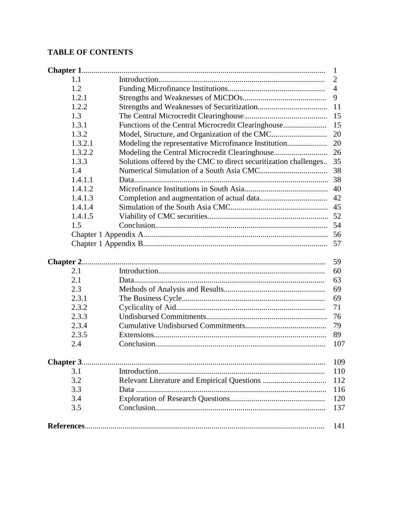
TABLE OF CONTENTS
Chapter 1........................................................................................................................... 1
1.1 Introduction.................................................................................... 2
1.2 Funding Microfinance Institutions................................................. 4
1.2.1 Strengths and Weaknesses of MiCDOs.......................................... 9
1.2.2 Strengths and Weaknesses of Securitization................................... 11
1.3 The Central Microcredit Clearinghouse.......................................... 15
1.3.1 Functions of the Central Microcredit Clearinghouse...................... 15
1.3.2 Model, Structure, and Organization of the CMC............................ 20
1.3.2.1 Modeling the representative Microfinance Institution.................... 20
1.3.2.2 Modeling the Central Microcredit Clearinghouse........................... 26
1.3.3 Solutions offered by the CMC to direct securitization challenges.. 35
1.4 Numerical Simulation of a South Asia CMC.................................. 38
1.4.1.1 Data.................................................................................................. 38
1.4.1.2 Microfinance Institutions in South Asia.......................................... 40
1.4.1.3 Completion and augmentation of actual data.................................. 42
1.4.1.4 Simulation of the South Asia CMC................................................. 45
1.4.1.5 Viability of CMC securities............................................................. 52
1.5 Conclusion....................................................................................... 54
Chapter 1 Appendix A............................................................................................. 56
Chapter 1 Appendix B............................................................................................. 57
Chapter 2........................................................................................................................... 59
2.1 Introduction.................................................................................... 60
2.1 Data................................................................................................ 63
2.3 Methods of Analysis and Results................................................... 69
2.3.1 The Business Cycle........................................................................ 69
2.3.2 Cyclicality of Aid........................................................................... 71
2.3.3 Undisbursed Commitments............................................................. 76
2.3.4 Cumulative Undisbursed Commitments......................................... 79
2.3.5 Extensions....................................................................................... 89
2.4 Conclusion...................................................................................... 107
Chapter 3........................................................................................................................... 109
3.1 Introduction.................................................................................... 110
3.2 Relevant Literature and Empirical Questions ................................ 112
3.3 Data ................................................................................................ 116
3.4 Exploration of Research Questions................................................ 120
3.5 Conclusion...................................................................................... 137
References......................................................................................................................... 141

1
Chapter 1
The Central Microcredit Clearinghouse:
Facilitating a Microloan Securitization Market
Chapter Summary
As Microfinance Organizations (MFIs) gain commercial viability, the prospect of international
capital markets' participation in assisting MFIs to meet the worldwide demand for services holds
much promise, especially in the area of microcredit. Prior analyses support the use of
collateralized debt obligations (CDOs) for bundling diversified loans to MFIs together to be
repackaged as rated investments. In this paper, I design a mechanism to aid in securitization of
microloans, using a dynamic investment pool governed by a Central Microcredit Clearinghouse
(CMC), that would sell investment units back to MFIs and outside investors simultaneously. The
CMC would serve as a catalyst to this other avenue of microcredit financing, securitization of
microloans, which could help spawn the type of growth in investor-based funding of MFIs that is
so urgently needed. Finally, I present a simulation of growth of microlending in South Asia, if a
South Asia CMC would have been in place for a ten year span.
2
1.1 Introduction
The microcredit industry, the largest component of microfinance services, is expanding in
volume, and close to reaching commercial viability. What started as a charitable mission
decades ago is moving from the purview of NGOs to the interested eyes of profit-seeking
investors. Recent years have seen rapid growth in micro-lending, advancing from an estimated
$4 billion market in 2001 to around $25 billion in 2006 (Dieckmann, 2007). Today, it is
estimated that over 100 million micro-borrowers in more than 85 countries are being served by
10,000 microfinance institutions (MFIs) (Galema & Lensick, 2009). These institutions
collectively self-report a gross loan portfolio of over $60 billion today (The Mix).
Despite this rapid growth of funds available to micro-borrowers, only around 4% of the total
demand for microloans is being met (Wardle, 2005; CGAP, 2006; Swanson, 2007; Byström,
2008; World Bank). It has been estimated that 1 to 1.5 billion potential micro-borrowers
collectively seek to borrow between $300 billion and $500 billion. The market appears to be in
disequilibrium, exhibiting significant and persistent excess demand (Dieckmann, 2007). If the
microfinance industry is to meet this demand, it must undergo significant adjustments, one of
which is increased access for MFIs to market-based funding sources.
The benefits of microfinance have been subject to significant analysis and scrutiny. Prior
research suggests that microcredit may not be a solution for impoverished individuals to lift
themselves out of poverty, since not every impoverished person possesses sufficient education or
entrepreneurial talent to create a successful enterprise. Another challenge to the effectiveness of
microlending is the ultimate use of funds. There is evidence that even with the thus far restricted

3
access to microloans, some borrow for consumption smoothing, instead of income generating
activities (CGAP, 2010; Amendariz, 2000).
However, it is most common for a micro-borrower to use funds in some domestic enterprise,
where the project return exceeds the interest cost of the loan, providing the borrower with an
income stream (Morduch, 1999). There is substantial evidence of microcredit's success in
alleviating poverty. There is also substantial evidence that many MFIs are able to hold defaults
to a sufficiently low portion of their loanable funds, keeping them operationally sustainable.
These together suggest that it is fair to set aside the discussion of microcredit's efficacy, and
continue on to the discussion of the development of microcredit markets.
One question of particular importance to the development of the industry is whether potential
funding sources for microloans are going unexplored. Microcredit financing as a debt-based
investment presents many challenges to be addressed before markets will adequately develop.
While loans to Microfinance Institutions (MFIs) constitute a large portion of their collective
working capital, another potentially lower-cost form of capital remains unavailable. Microloan
securitization has been briefly and recently attempted, but with poor results. Weaknesses of a
microloan securitization market are plentiful both from the point of view of the investor and of
the MFI.
For the investor, the lack of corporate governance in smaller MFIs, currency risk, country risk,
non-standardization of accounting practices, and lack of institutional oversight all collude to
provide risk that is most often uncompensated by the return potential. For the MFI, the cost of

4
securitization is prohibitive (Pollinger & Outhwaite, 2007). While such a market could provide a
rich, new source of lower-cost funding for expansion of microlending to poor areas, the financial
expertise required would be substantial. Even more threatening is the combination of this cost
with the term of the typical microloan. Loans of just a few months are paid off almost as soon as
they could be securitized, so that the expensive process would need to be repeated far more often
than for mortgage-backed securities, for example. The purpose of this paper is to propose a
solution to some of these challenges, so that market funding can expand for those MFIs in
position for survival, growth, and eventual market penetration.
The remainder of the paper is organized as follows: Part 2 provides a survey of the current
literature concerning funding sources and capital market access to MFIs, including the
Microcredit Collateralized Debt Obligation (MiCDO) market, and the relative strengths of the
main forms of capital market funding for MFIs. Part 3 introduces a hypothetical organization
called the Central Microcredit Clearinghouse (CMC), and discusses its purpose in facilitating
securitization of microcredit loans, as well as its potential organization and operation. Part 4
then uses data available about South Asian MFIs to present a simple numerical example of how a
South Asia Central Microcredit Clearinghouse (SACMC) might have assisted in development of
regional MFIs to expand their services over a ten year span. Part 5 concludes.
1.2 Funding Microfinance Institutions
The many microfinance institutions (MFIs) operating worldwide vary widely in their capital
structure1. The mission of microfinance as a means toward poverty alleviation appeals to a large
1 Fehr & Hishigsuren (2004) provide a detailed listing of operational funding sources for MFIs.
5
group of individual and institutional donors. Donations constitute a large share of operational
dollars to many MFIs, as do government grants, and subsidized lending (Fehr & Hishigsuren,
2004). Although some MFIs are moving toward independent financial sustainability, for the
industry of microfinance as a whole, donations and grants have been, and continue to be, a
necessary support.
Client deposits often constitute a significant percentage of total liabilities for financial firms
(Hempel & Simonson, 1999), and many MFIs are choosing to go beyond microlending by
allowing, and even sometimes mandating, savings accounts held by clients of microcredit.
Dowla & Alamgir (2003) describe the evolution of savings instruments in Bangladesh, noting
that, despite regulatory challenges, these savings instruments not only provide liquidity to the
MFIs, but also grant some protection against defaults. Of the more established MFIs in South
Asia, for example, two-thirds report holding savings accounts of clients, which total an average
of about 25% of assets (The Mix).
A table of microfinancing evolution typical to MFIs is provided by Calvin (2001) and modified
by Fehr & Hishigsuren (2004). It shows the early MFI supported mainly by donations, savings
of clients, and government grants. Various forms of debt financing are sought by more mature
MFIs, and in the final stages, equity financing becomes part of the balance sheet. This equity is
comprised of retained earnings, social-minded equity stakes, both private and institutional, and
even commercial equity in the case of the strongest and most viable MFIs.
6
While donations and grants can get a young MFI into operation and sustain it for some time, few
have reached the point of commercial viability where traditional equity investing is possible. An
intermediate funding source, and also the most widely used, is debt. MFIs who have reached a
certain point of stability as an ongoing concern are finding themselves eligible to secure funding
in debt markets. Debt financing is the main focus of this paper, and it can be further subdivided
into classes of direct borrowing and intermediated (brokered) transactions. Direct borrowing is
straightforward; if an MFI can sometimes borrow from another financial institution for
operational financing. However, due to the small size of most MFIs, the high transactions costs
facing lenders associated with funding at the individual level makes this impractical (Glaubitt et
al., 2009).
In contrast to direct loans, some borrowed funds are acquired indirectly, via intermediation
through either packages of loans made to a group of MFIs, or securitization of microloans. It is
this second category of financing that is the focus of the rest of the paper. The recent history,
present status, and potential future realizations in the microcredit market is summarized by
several authors (see, for example, Byström 2008). In his work, Byström introduces the
Microcredit Collateralized Debt Obligation (MiCDO), and argues for its use as a conduit through
which MFIs and Wall Street investors can meet. Such a rapid growth in total volume of
microcredit worldwide has allowed MFIs to provide attractive opportunities to investors. That
is, markets for CDOs require a deep enough pool of underlying assets for diversification, for
proper valuation, and for replenishment of matured securities.
7
As a semantic distinction, Galema & Lensink (2009) use "CDOs" to refer to pooled loans
granted to MFIs, with resulting securities backed by the MFIs themselves, and "securitization" to
refer to marketing of securities backed purely by specified microloans. For the purposes of this
discussion, I will follow this convention. Microfinance Collateralized Debt Obligations
(MiCDOs) will signify the group-MFI lending by investors via intermediaries, and
"securitization" will signify either a direct microloan to investment security conversion, or a
securitization of microloans performed by an intermediary.2
Several authors foresee a growing and strengthening microcredit collateralized debt obligation
(MiCDO) market (Byström 2008, Sundaresan 2008, Swanson 2007).3 In fact, loans of this type
have already occurred in recent years.4 The Dexia microcredit fund was launched in 1998,
aimed at the provision of financing to MFIs providing services to small businesses. More
recently, in 2004 the BlueOrchard Microfinance Securities I fund (BOMSI) was launched. This
was a new type of funding strategy for the field, loaning over $80 million directly to 14 MFIs,
and the pooled debt was sold in Senior, Subordinated, and Equity tranches to investors (Swanson
2007). This is arguably the first real MiCDO, and its degree success will be of interest. Many
microcredit funds have been launched in the interim,5 allowing investors another indirect avenue
2 MiCDO itself is a misnomer, since nothing is collateralized in MFI lending. These loans are
simply debenture loans granted to MFIs, and backed only by their own good faith. 3 News of MiCDO developments are important additions to any published work; the reader is
referred to the MIX market (www.themix.org), the World Bank website, and other microfinance
and microbanking bulletins for current information on what is summarized here. 4 ProFund was a specialized Microfinance Investment Vehicle (MIV) that started in 1995, raising
$23 million in an effort to finance several Latin American MFIs. For more on this, see
Dieckmann (2007). Some evolutionary details in this storyline leaves debate as to how we might
define the true start of the MiCDO. BOMS1 is considered by many to be the first. 5 As of the time of this writing, www.microcapital.org provides a listing of at least 27 funds that
specialize in providing funding to microfinance institutions.
8
to funding micro-borrowers; providing liquidity to the organizations that loan to the
impoverished.
The operational sustainability of MFIs is necessary for this trend to continue. As long as
MiCDO investors are realizing a fair risk-adjusted return, MFIs may use this access to funds to
continue operation and expand services. It may be true that, in time, indirect MiCDO funding of
MFIs will provide the needed capital for eventual market saturation. Many look to this avenue
as the predominant form of structured microfinance in the near future.
Securitization has only been attempted in reduced form. What was touted as the first and largest
"microloan securitization" deal was really a "microloan purchase" (Swanson 2007). SHARE
Microfin Ltd. is the third largest MFI in India by microloan volume, with over 1,000 branches,
specializing in microcredit loans to poor women across India. In January 2004, $4.3 million of
SHARE's microloan portfolio6 was purchased by ICICI Bank (Basu, 2004). This was a direct
transfer of receivables, and can be viewed as a securitization deal where ICICI Bank retained all
shares. ICICI Bank is India's largest commercial bank, and the deal was guaranteed by the
Grameen Foundation, providing technical assistance and a collateral deposit of $344,000. The
securities were purchased at a net present value, allowing SHARE to pay a rate of 8.75%, which
was over 3% less than the rate of commercial loans (IFMR, 2007). Also, a second securitization
deal was made between ICICI Bank and BASIX in 2004 for $842,000 of its microloan portfolio.
6 According to The Mix Market (www.mix.com), SHARE maintained about $44 million in loans
in 2004, making this offering about 10% of its total portfolio, even though it was 25% of total
loans, indicating that it was truly a microloan transfer. These loans were simply assumed by the
bank, not securitized and resold to investors as in a traditional securitization deal. (To
underscore the impressive and continued growth in this industry, SHARE's microloan portfolio
grew from $44 million in 2004 to over $576 million in 2009, just five years later).

9
While these transactions appear to hint at a developing securities market for securitized
microloans, positive reports of the ultimate profitability of these microloan purchases are hard to
come by. An acceleration in microloan purchases is not evident, and many reasons for this are
enumerated in the following section.
1.2.1 Strengths and Weaknesses of MiCDOs
The recent surge of support of MiCDOs from stakeholders in microfinance arguably stems from
its current and potential volume. Until recently, there simply wasn't a great enough volume of
microcredit origination to warrant its consideration as a viable asset class. Now that this
aggregate has crossed $25 billion (Dieckmann, 2007), the possibilities have changed. The
potential profitability of top tier microlenders has caught the interest of the investment
community. While attainment of this new market volume level is the main catalyst for this
progression, there are several other reasons why MiCDOs can be mutually beneficial for MFIs
and their investors.
As an asset class, packages of microloans (or packaged loans to regional groups of microlenders,
to stay within the MiCDO framework for now) would provide an investment that is fairly
homogenous, subject to little prepayment risk, and resilient to economic shocks (Dieckmann
2008, Galema & Lensink 2009). MiCDOs could certainly present investors with an attractive
risk-adjusted return, if default rates remain as stable as are widely reported for the more
successful MFIs. Loans to a handful of MFIs would also provide some diversification to the
10
investor. However, the security would retain significant firm risk, since these loans are repaid by
and backed only by a small group MFIs.
For many investors, part of a "return" on their investment includes personal benefits, such as
knowing that they hold a Socially Responsible Investment (SRI) (Morduch 1999, Copestake,
2007, Dieckmann 2008). Since some poverty has been alleviated by coupling entrepreneurial
ability and drive with initial financing, investors in MFIs or their constituent clients are indirectly
providing that opportunity to some of the billions of impoverished citizens of our globe.
Marketing MiCDOs as an SRI may enhance investor interest in the asset class.
While financialization techniques and market sophistication have evolved significantly in past
decades to easily assimilate a new asset class, Wall Street investors are used to a well-regulated
market. Once we consider the debtors in a MiCDO as a small organization in south Asia, Africa,
South America, etc. it is easily imagined how these standard rules of the developed world may
not apply. To provide investors with better assurances and become eligible for MiCDO funding,
many MFIs will have to improve their corporate governance (Arun & Hulme 2008, Glaubitt et
al. 2009, Swanson 2007).
In some countries, currency and inflation risk is significant. In places that suffer economic
instability as a direct result of macro policy, the total risk presented to the foreign investor may
simply be too great (Byström, 2008). Currency risk is often viewed as a source of diversification
to investors, but the risk of currency devaluation amid hyperinflation is universally unwelcome.
This potential currency risk could significantly slow the development of international capital
11
markets tailored toward microfinance (Byström, 2008, Swanson 2007). For many investors, the
ability to effectively hedge this risk is essential. Donated funds also represent a threat to the
growth of commercial MFI financing. Many microlenders are just beginning the transition from
NGO to a profit-seeking, financially sustainable organization. Donor funds will need to be put to
use in ways other than direct MFI funding, or else some activity will be crowded out by this free
financing (Byström 2008, Glaubitt et al. 2009).
In summary, MiCDOs present investors with a possibility of fair risk-adjusted returns,
diversification, and the added benefit of being a reasonable social investment. Also, developed
financial markets have the tools to effectively financialize these investments. Challenges that
remain include a weak legal and regulatory environment with idiosyncrasies across each border,
macro policy challenges, country-specific, currency risk within each MiCDO that is not regional
in nature, currency risk for the foreign investor even if only one currency is used for loan
denomination, and the threat of donated funds "crowding out" profit-seeking efforts necessary to
grow the industry to meet demand.
1.2.2 Strengths and Weaknesses of Securitization
The direct securitization of microloans is another way that investors can connect with
impoverished borrowers. It is this conduit to liquidity that now takes center stage in the
discussion. Early attempts at securitization, as noted earlier, have not been successful. It is vital,
then, that the strengths and weaknesses of securitization are analyzed, in search of a better
method of securitization, if it is to be used at all in MFI financing.
12
Attractive investments with an infrastructure to create them
As with MiCDOs, securitizations can offer investors a fair risk-adjusted return (even greater,
when enhanced diversification is realized). They are also classified as a Socially Responsible
Investment (SRI), and the investor of a securitized portfolio is able to take on the good faith of
an individual or small group of impoverished borrowers instead of vouching for the general
operations and activities of an MFI. Also, the same developed markets that can create MiCDOs
stand ready to establish securitization contracts. In addition, there are reasons to prefer this form
of risk transfer to MiCDOs. First, investors are offered a "pure play" on the underlying asset,
instead of relying on the viability of the MFI (Swanson, 2007). The microloans as a pooled and
securitized asset are vastly diversified, much more so than loans to a handful of organizations
(Glaubitt et al, 2009). Since securitized investments have their underlying value in the
microloans themselves instead of the MFI, there is little firm risk.
Reduced liquidity strain for the MFI
Also, one marked benefit of securitization over MiCDO funding is the removal of liabilities from
the balance sheet of the MFI. Cash via a MiCDO provides extra liquidity, a portion of which can
be loaned out. This in turn expands leverage ratios, making the MFI more risky as a going
concern. When required rates of returns on loans to that MFI increase, the benefit is mitigated.
Securitization allows for the sale of the receivables for cash without exacerbating the firm's
leverage ratios. This allows for further originations and subsequent sales, never forcing the MFI
to approach an operational limit due to excess leverage.
13
However, these improvements come with a price. It is straightforward to review the list of
MiCDO challenges in section 2.1 and recognize that they also apply to securitizations. The same
legal risk, macro instability, and other challenges face direct securitizations of microloans in the
traditional framework. In addition, securitization presents an addendum list of obstacles to
overcome.
Extremely Short-term Loans
A common securitization in developed markets is based on mortgage loans, with terms of 15-40
years. These loans can be packaged relatively infrequently, and allowed to perform over this
time frame. In contrast, many microloans are as short in term as just a few months. Packaging
these short-term loans for securitization would present the financial intermediary with
significantly higher (i.e. more frequent) administrative costs than other securitizations, much as
the MFIs wrestle with similar costs at origination. This is a significant threat to the growth of
any microloan securitization market (Byström, 2008, Swanson 2007).
Lack of Financial Sophistication in Small MFIs
There is significant technical, relational, and legal expertise required of an MFI to securitize its
loans. While it is true that many of these skills could be acquired in the market by using
financial intermediaries, still there remains a need for knowledge and advocacy at the MFI level
if a series of successful securitizations is to take place. Most of the 10,000 MFIs in existence
would find themselves inadequately supplied with these resources (Glaubitt et al., 2009).
14
Moral Hazard
The originating MFI plays a substantial role in the local success of the microcredit market. The
relationships built and social pressures utilized in exacting repayment are vital to the success of
microlending (Swanson 2007). These ongoing efforts are very costly for the MFI. Also,
securitization passes the risk of the loan from the MFI to the investor. Therefore, there is a great
incentive to, after origination, let securitized loans perform without these efforts. Potentially,
moral hazard exists at the borrower level as well. The close relationship necessary between an
MFI and its client indicate significant communication between the borrower and the MFI
representative. The market's solution to the problem of these higher default rates would be to
sever the relationship between foreign investors and MFIs once risk-adjusted returns fell
sufficiently, making future securitizations (even if improvements were undertaken) much more
difficult. In this way, moving too quickly into securitizations could quite possibly even harm the
evolution of the market into longer term practices.
Summary
The additional costs presented by traditional loan securitization over that of MFI-level CDOs in
microloans clearly outweigh the benefits of occasional investor preference and added
diversification. It is this direct comparison that have led many to abandon microloan
securitization as a promising possibility. Still, the benefits of a promising avenue of funding, the
creation of an attractive investment-grade asset, and the reduction of leverage from the balance
sheets of MFIs are worth pursuing. Success might rely on the existence of a custom designed
intermediary available to address the challenges that currently stifle any microloan securitization
market.

15
1.3 The Central Microcredit Clearinghouse
In this section, I propose the formation of an entity that can address most, if not all, of the
challenges identified here to direct securitization of microloans, and in fact provide multiple
enhancements to the market as well. Where traditional securitization techniques fall short in
terms of cost-effectiveness, risk management, and practicality, a specific type of structured
finance closely approaches the level of innovation that may succeed in developing this market.
Multiple types of Asset-Backed Commercial Paper (ABCP) structures exist in developed
markets. One is the multi-seller structure, allowing multiple originators to combine assets in a
securitization through program sponsor that then sells homogenized securities to investors in the
market. The proposed entity, the Central Microcredit Clearinghouse (CMC), is a regional
clearinghouse for microloans set up to serve several potential functions, some of which are
similar to the role played by the sponsor in an ABCP securitization. In the following sections,
the multiple purposes, the organization, the operation, and the solutions offered by a CMC will
be explored.
1.3.1 Functions of the Central Microcredit Clearinghouse
The main function of the CMC is to stand ready to purchase microloans from member MFIs.
While securitizations are most often large brokered deals (and often guaranteed by a third party),
a microlender would be able to sell small to medium-sized batches of loans directly to its
regional CMC for an actuarially discounted value, based on several criteria. In this way, the
CMC would serve the purpose of both the Special Purpose Vehicle (SPV) and sponsor in
traditional securitizations, but without the need for exclusivity to one particular originator, and

16
not for securitization of just one set of microloans. The regional CMC would offer purchase
agreements to any area MFI that met certain membership criteria, with each purchase made at the
option of the participating MFI, facing independent and automated valuation.
This valuation might be a function of the MFI's star rating on the Mix Market, the performance
of past loans sold to the CMC, and the percentage of CMC securities held by the MFI of total
assets under management7. Inclusion of the Mix market rating is simple.
8 If the MFI has a five
diamond rating, then they are afforded a nonzero value for some binary variable in the valuation
equation. This will serve as an encouragement for the MFI to pursue the extra rating or due
diligence report required for this fifth diamond, as well as the incentive to maintain that rating.
Performance of past loans sold to the CMC would be vital in assessing the MFIs' ability to
service current loans and the clients who receive them. A ratio of currency received to currency
loaned could easily be calculated for each interest rate level, loan size, and demographic
variables relating to the borrower. This would provide the CMC with a good estimate of a mean
repayment rate for each future loan purchased from an MFI. Using this information as a large
portion of the purchase value of the loan would be one very important step in addressing the
enormous moral hazard problem that plagues traditional securitizations, where the originator
could pass along poor loans for excess profit. Such a scheme would not be beneficial for an MFI
7 As indicated in some areas below, a successful valuation will ultimately be more complex,
including some variables for country risk, currency risk, inflation expectation and firm financial
ratios at minimum. 8 The CMC would likely accept only four- and five-diamond rated MFI loans. The Mix Market
assigns a 1-5 diamond rating to an MFI based on disclosure levels, and four diamonds are given
once the MFI has at least two consecutive years of audited financial statements with an auditor's
opinion and notes.

17
in the long run, and they would likely be competed away by more stable MFIs. In addition,
initial sales of loans to the CMC by a newly participating MFI could be restricted to small
amounts, until some accredited payment history is established.
Third, using a purchase ratio of CMC securities and cash to the total of receivables purchased is
a way to mitigate moral hazard. Since the sale of microloans to a regional CMC allows an MFI
to free up more cash for origination of additional loans, a constant pass-through of loans with no
minimum holding percentage would essentially allow the MFI to quickly multiply its cash into a
massive expansion of loans.9 Instead of assuming this risk, the CMC would purchase loans for a
combination of cash and CMC-securitized assets, to be held at the CMC in the name of the MFI.
Purchasing microloans from MFIs would bridge a large portion of the current funding gap; but
the CMC is not a central bank, and cannot create money from nothing. This organization will act
more like a broker between profit-seeking investors, and MFIs with a comparative advantage in
local lending. Securitization of these microloans, in a style similar to that of investment banks,
will allow the CMC to repackage and sell this debt both back to the MFIs it serves, and to
domestic and foreign investors.
By assessing the repayment risk, any country risk, inflationary pressure, etc. at the point of
purchase, the CMC could then actuarially reduce each loan to an expected CMC currency unit
(CMCU). This currency unit would be denominated in the most internationally traded currency
9 This would incite a one-time moral hazard for a small MFI. Without limits, loans could be
originated, immediately sold for cash to the CMC, and re-originated any number of times in a
single day. The MFI could then cease CMC membership, while hundreds or thousands of
"clients" default.
18
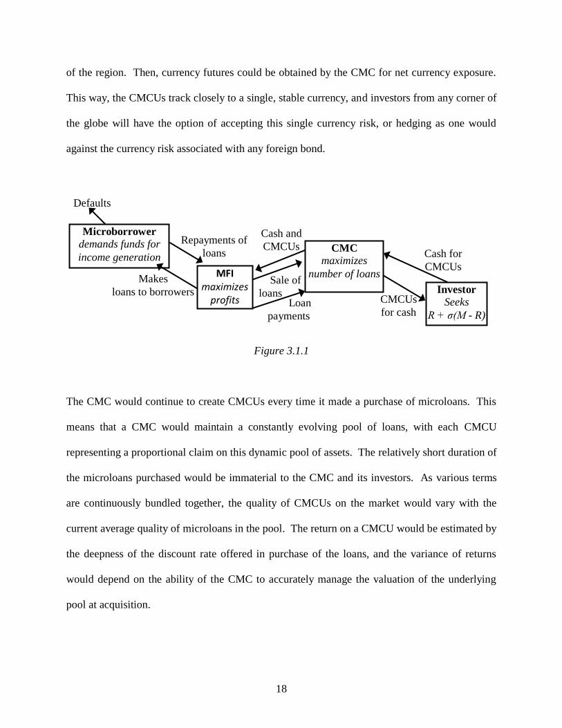
of the region. Then, currency futures could be obtained by the CMC for net currency exposure.
This way, the CMCUs track closely to a single, stable currency, and investors from any corner of
the globe will have the option of accepting this single currency risk, or hedging as one would
against the currency risk associated with any foreign bond.
Figure 3.1.1
The CMC would continue to create CMCUs every time it made a purchase of microloans. This
means that a CMC would maintain a constantly evolving pool of loans, with each CMCU
representing a proportional claim on this dynamic pool of assets. The relatively short duration of
the microloans purchased would be immaterial to the CMC and its investors. As various terms
are continuously bundled together, the quality of CMCUs on the market would vary with the
current average quality of microloans in the pool. The return on a CMCU would be estimated by
the deepness of the discount rate offered in purchase of the loans, and the variance of returns
would depend on the ability of the CMC to accurately manage the valuation of the underlying
pool at acquisition.
Microborrower
demands funds for
income generation
MFI maximizes
profits
Makes
loans to borrowers
Defaults
Repayments of
loans CMC
maximizes
number of loans
Investor
Seeks
R + σ(M - R)
Cash and
CMCUs
Sale of
loans
Cash for
CMCUs
CMCUs
for cash Loan
payments
19
The CMCU has several attractive qualities as an investment. It would be well diversified across
borrowers, representing the collective repayments of all micro-borrowers of a region. It would
be valued and created independently by a nonprofit institution, with the mission of developing
the investor-MFI connection through this indirect securitization channel, making it relatively
easy and transparent for investors to value. The social nature of the investment would remain, as
the investor not only receives a nearly direct connection with the micro-borrower, but also
indirectly supports the CMC with social objectives other than just investment brokering, to be
described below. Finally, a CMCU would be denominated in a single, stable, and hedgeable
currency.
Another useful function of the CMC is the provision of various standards of membership,
governance, accounting & reporting practices, emergency financial assistance, and arbitration.
The number and variety of microlenders in existence leaves potential investors with a dizzying
array of information to assimilate. Accounting practices vary widely, language barriers hinder
communication, cultural norms require lenders to practice in different ways, with different rules;
this leaves significant heterogeneity in microloan receivables. It also leaves potential direct
investors (large banks willing to accept loan packages, much like the ICICI purchase of 2004)
wary of the counterparty risk.
Finally, the CMC, through its incentivized loan purchase and securitization program, could
actually serve to provide a little creative destruction to the field. That is, the influence of the
CMC could serve to grow the most successful microlenders, and at the same time, be a catalyst
for some healthy crowding out of other microlenders who are already losing money, are
20
inefficient, or practice lending with methods that are ineffective or harmful to the client. The
acceleration of funding to MFIs in the field may also accelerate the market's ultimate response.
1.3.2 Model, Structure, and Organization of the CMC
In this section, I intend to briefly introduce some of the possibilities in organizing a regional
CMC. In section 4, I assume a South Asia CMC, and create a dataset to simulate ten years of
activity. This will show some of the potential direct benefits of the existence of a South Asia
CMC (SACMC). This section is written with this area in mind, although the structure here is
flexible enough to export to every region of the world.
1.3.2.1 Modeling the representative Microfinance Institution
Assume there is a representative microfinance institution (MFI) in a geographical region. There
is demand for loaned funds from n identical potential micro-borrowers in that region.
Transportation costs for borrowers to get to another MFI are prohibitive. All n borrowers have
potential entrepreneurial projects with chances of success of known probability, and other
potential sources of income or lending sources for repayment of MFI loans.10
The combination
of these factors (as well as the performance of the MFI in project development and collection
activities) creates a probability of default, d, where with probability 1 - d, the MFI's loan will be
paid in full, including interest charges. For simplicity, I assume that if a borrower defaults, they
will do so immediately after origination. It is also reasonable to assume that the default rate is an
increasing function of the interest rate chosen by the MFI. Therefore, the probability of default
is d(I), where I is the monthly interest rate, and dI > 0.
10
The borrower is often more richly modeled in other settings, where adverse selection, strategic
default, etc. are of interest. Here, the focus is on the lender; the borrower will remain simplified.
21
Each identical representative borrower seeks a loan of size g. The loan demand function is g(I),
g(I) = 0 for some finite level of I, and gI < 0. Total demand of loanable funds facing the
representative MFI is then LD = ng(I).
Each loan has an identical term of m months. The payment expected from each borrower at time
t is given by
Idm
IIgPE
m
t
11
. That is, interest for the term is entirely expensed by
the borrower at origination. This is known as a "flat rate" calculation, and is common practice
among MFIs in developing nations. It removes the prepayment incentive, and also creates an
APY much larger than the stated interest rate.
Each MFI is endowed with initial cash on hand of C0, and inelastically supplies this cash to the
market in lending each period. The MFI is able to borrow from capital markets at some rate rMFI,
which is an exogenously determined rate greater than a net risk-free periodic rate R. From this,
the MFI chooses a debt level in each period of Dt.11
The supply curve of the representative MFI
is then the perfectly inelastic curve of originations Ot = Ct + Dt.
Each MFI has a fixed cost w of originating a new loan that is recognized at the time of loan
origination. This can be assumed to capture necessary search costs, screening, documentation,
and all administrative expenses, including subsequent collection and processing of payments.
Since the MFI originates a total loan portfolio addition of Ot in each period, lending to Ot/(g(I) +
11
Perhaps rMFI = (R + σROA(M-R)/σM)*(1+Debt/Equity ratio of the MFI), for example. The
specific rate is beyond the scope of this paper, and does not impact the subsequent analysis of
interest, which surrounds the CMC.

22
w) borrowers, with origination expenses of wOt/(g(I) + w) in each period. Each MFI is able to
costlessly invest any cash on hand to earn the periodic risk-free net return R.
If we allow the MFI to choose an interest rate in the face of their cash constraint and origination
cost, the MFI will have cash in each period Ct of
(3.2.1.1)
1
1
1 11
1
tMFItt
t
mtk
m
ktt DrDwIg
w
wIg
IgOId
m
IORCC
That is, the ending cash balance in each period after zero is the ending cash balance from the
prior period plus its investment income, plus the sum of payments net of defaults from the
current period and the m-1 prior periods on past loans, less new originations and related costs,
plus any debt held, minus any debt service payments.12
Also, assume that the MFI does not offer
deposit accounts. This removes a money multiplier effect from loaning its initial cash.
Further assume that Ot < ng(I) for all "reasonable" levels of I; that is, there is excess demand for
loans.13
Recall the origination fee w. It is this variable that disallows an equation of Ot = ng(I).
Indeed, if w = 0, then the MFI could simply loan tiny amounts of cash to each potential micro-
borrower with demand for a loan, charging a high enough interest rate such that the market was
in equilibrium. To maintain excess demand for loanable funds, it is sufficient to assume that Ot
< wn.
Equation (3.2.1.1) creates a trade-off for the MFI: higher interest rates bring in higher payments
12
See Appendix A for more on this decision. In subsequent discussion here, incoming cash each
period of
1
11t
mtk
k
m
k dm
IO
will be occasionally substituted for Ct for notational ease.
13 The inclusion of w will be shown at the end of this section to limit the range of interest rates
chosen by the MFI.
23
in a given loan, but it also incentivizes smaller loan sizes given that gI < 0, increasing the cost of
origination as a percentage of assets under management. Also, to simplify calculations, we will
allow for "fractional loans" instead of rounding to the nearest whole optimal loan value.14
The MFI has no incentive to hold on to cash in each period, if demand is sufficient to make
lending worthwhile. There are no liquidity reserve requirements, and no assumption of liquidity
risk for the MFI. So, the MFI has only capitalized interest and as total income, and origination
fees and potential debt service as total expenses. Idle cash is suboptimal; the MFI would prefer
to use any cash for operational returns in excess of R. Using (3.2.1.1), we can then allow prior
period cash and debt to be zero, and Ot = Ct. Then, solving for current period originations:
(3.2.1.2)
1
11t
mtk
m
kt Idm
IOO
Equation (3.2.1.2) tells us that the outflows in each period will equal the inflows. The payments
received on prior loans, which are the sum of outstanding loans and capitalized interest net of
defaults, are pooled and re-loaned, less the portion of the "loan plus fee" sum that is required for
origination expenses.
It is also important to specify that the MFI is assumed to be sustainable. At this point, only a
necessary condition is given. Any loan made by the MFI must be assumed to return in
expectation at least the undiscounted nominal cash equivalent over the term of the loan. If this
14
This is a fairly reasonable concession, given that the demand for loanable funds is downward
sloping. We assume that the MFI can find a borrower who then will take a loan at less than their
reservation interest rate for the smaller loan amount. This also allows the MFI to reduce
origination costs on this last fractional loan, which is also implicitly assumed in the calculations.
24
condition is not met, the MFI is simply granting, rather than microlending. This requirement,
then, is that expected repayments from period t+1 to period t+m sum to at least the sum of
originations and related costs in time t.
(3.2.1.3)
wIg
w
wIg
IgOId
m
I
wIg
IgOPE t
mt
tk
m
t
mt
tk
k
11
11
Since (3.2.1.3) sums across m periods of identical payments, the expression can then be
simplified:
(3.2.1.4)
111
IdI
wIg
Ig m
Equation (3.2.1.4) is simply a statement that the net return on loans must be greater than or equal
to zero. This provides both a lower bound and an upper bound for the interest rate choice by the
MFI15
. If the interest rate is too low, then interest income will not exceed the fixed origination
expenses, even though originations will be relatively few, and of relatively large size. If the
interest rate is too high, then the many small loans originated will generate too large a number of
origination expenses. Since the interest rate has both an upper and lower bound, the borrowers'
demand for funds g(I) is also constrained with an upper and lower bound. All that is necessary
to lead to a persistent disequilibrium is a sufficiently high number of borrowers n given the
parameters chosen.
15
This assumption is predicated on the existence of real roots for (3.2.1.4) with respect to the
interest rate. Since the expression is to the power of m, there are many potential roots. For
subsequent analysis, it is necessary that at least two real roots may exist, which is shown in
Appendix B.
25
Growth of the MFI
The gross growth rate of originations is simply 11/ tttt DCDC , And this gross growth
rate is provided by the left hand side of equation (3.2.1.4). Therefore, an MFI is expected to
grow at the gross rate of a growth factor (GF) given by:
(3.2.1.5)
dI
wIg
IgGF
m
11
which is a non-negative rate for the sustainable MFI (and at this point must be larger than R to
induce lending).
The MFI's profit is revenue, or
IgwIg
DCIdIIg
wIg
DC ttmtt
11 minus expenses, or
wIg
DCw tt
. Profit is then:
(3.2.1.6)
wIg
DCwIg
wIg
DCIdIIg
wIg
DC ttttmtt
11 .
We can simplify this expression, recognizing from the right side of the profit function that:
tttttt DC
wIg
DCwIg
wIg
DC
Profit is then, more simply,
(3.2.1.7)
tt
mtt DCIdIIgwIg
DC
11

26
To solve explicitly for the profit-maximizing interest rate, we assume linear demand16
IIg , and a linear default rate function IId .
Then, profit maximization for the MFI is the solution of:
maxI tt
mtt DCIIIwI
DC
11
A first order condition provides:
0
11111112
1
wI
IIIIIImIIIIwIDC
I
mmmm
tt
At this point, the denominator, cash, and debt all drop out. Also, 11
mI can be cancelled
throughout. This leaves a simplified expression:
(3.2.1.8) IImIIIIwI 1111
011 III
The I* that equates this expression is the optimal interest rate that the MFI will choose for profit
maximization. This rate also maximizes the MFI's growth factor:
(3.2.1.9)
*1*1
*
*IdI
wIg
IgGF
m
The choice of debt level follows immediately from this. If I* > rMFI, then the MFI will borrow
until I* = rMFI.
1.3.2.2 Modeling the Central Microcredit Clearinghouse
Assume now the existence of a nonprofit organization, with the goal of maximizing the number
16
Note that this assumption need not describe the entire demand curve. For purposes here, we
only need to assume linearity of demand within the limits of interest rate feasibility given by the
sustainability requirement of (3.2.1.4).

27
of loans in its service region. The main function of this organization, the Central Microcredit
Clearinghouse (CMC) is to allow the sustainable MFI to achieve the optimum growth rate shown
in (3.2.1.8) within periods, by augmenting its loan portfolio via a money multiplier maintained
by the CMC. Another main function of the CMC is then to securitize its resulting portfolio of
microloans, allowing investors a "pure play" on a standardized investment unit.
To see the leverage effect, consider the representative MFI that has just finished loaning its cash
balance of Ct in time t. With many other potential borrowers waiting, the MFI is forced also to
wait until payments arrive in period t + 1 to sum to Ct+1, so that another period of lending can
ensue. However, now assume that the regional CMC is in operation, and the representative MFI
is approved as a member agency. The CMC now stands ready to purchase the portfolio of
microloans from the MFI at an actuarially determined rate of p times the expected value of the
portfolio, where 0 < p < 1. A fraction 1-f is purchased for cash, and the remaining fraction f is
purchased for investment units in the pool of underlying loans at the CMC, maintained at the
CMC in the name of the MFI. It is the CMC's choice of the values of p and f that allow it,
indirectly, to influence the number of loans granted.
The discounted purchase rate p ensures that some expected value is passed on to investors of the
resulting CMC securities, and this total expected gross return is 1/p. Therefore, the MFI is left
with the choice in each period to invest cash in an outside risk-free investment with gross
periodic return R, a risky market asset M, invest in borrowers with gross periodic expected return
*1*1*
*IdI
wIg
Ig m
, or to connect microborrowers to the CMC by originating
microloans, selling the receivables to the regional CMC for an immediate gross return
28
*1*1*
*IdI
wIg
Ipg m
on portion 1-f of the sale, receiving CMC securities for f portion
of the sale, and reinvesting the cash in more microloans, effectively leveraging the portfolio by a
calculable multiplier.
The summation of these repeated loan balances, reduced in each round by the fraction 1 - f and
augmented by the growth factor net of purchase
IdI
wIg
Ipg m
11 are a geometric
series, leading to a Maximum Leveraged Growth Factor (MLGF) of
(3.2.2.1)
IdI
wIg
Ipgf
IdIwIg
Ifpg
MLGFm
m
1111
11
From (3.2.2.1), it is unclear whether MLGF > GF. This depends on, among other things, the
value of p. If the CMC pays a purchase price that is "too low", it is reasonable that the MFI
would be better off originating microloans for itself without partnering with the CMC. Given the
securities ratio f, there exists some price pmin for the CMC that makes MLGF = GF. This can be
found from (3.2.2.1) as
(3.2.2.2)
IdI
wIg
Igff
pm
111
1min
The CMC must offer a purchase rate greater than pmin to induce sales by the MFI. This allows a
maximum return to the investor of CMC securities of the inverse of (3.2.2.2). It is quite possible
to have a sustainable MFI where (3.2.1.4) holds (i.e., FG > 1), and yet the MFI does not engage
in lending because FG < R. However, for purchase levels p > pmin, we know that MLGF > GF
(where GF > 1). This allows for the condition MLGF > R > GF. In this case, the presence of
29
the CMC allows the MFI to sustainably lend, where it would not on its own. However, this
would require concessionary investing, as the return 1/pmin would necessarily be less than 1+R.
Regardless, this possibility exists with the leveraging effect offered by a CMC.17
The sustainable
and active lender, where FG > R, is able to grow at the faster rate of MLGF when p > pmin.
The discount factor p is also bounded from above. The CMC is assumed to get its funding from
investors, who demand an expected gross return 1/p that is at least the rate compensated for the
amount of risk (measured in standard deviation of returns) that the CMCU presents. Assume that
investors demand a return provided by the standard Capital Market Line (CML) as:18
(3.2.2.3) MCMCU RMRp
p /
1
A higher f reduces the expected variance of the investment return, also working to satisfy the
constraint, but lowers the MLGF. The assumed relationship that links the leveraging factor f to
the risk factor σCMCU is simply σCMCU = (k/f)σM, where k is some scalar to account for the
assumed relative variance of the CMC security and the market portfolio, given the default
multiple of 1/f.
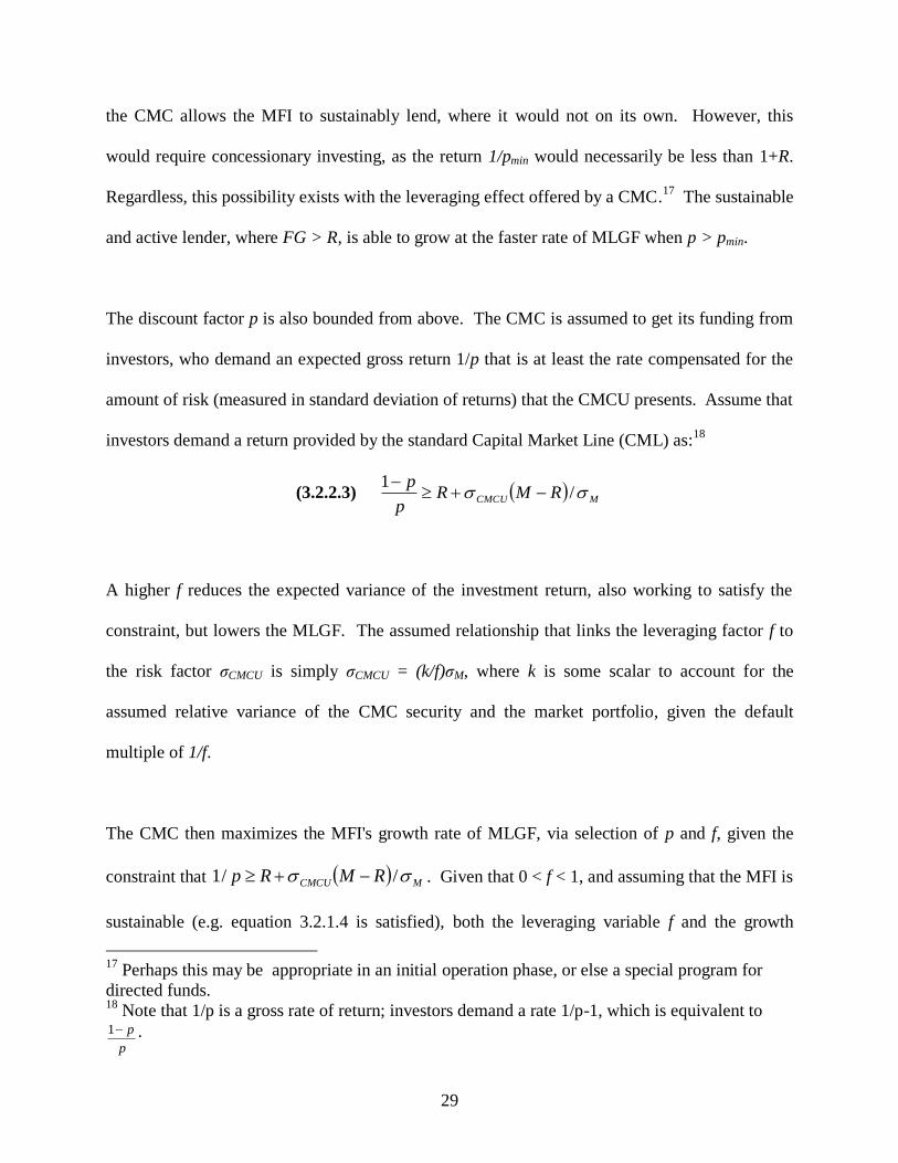
The CMC then maximizes the MFI's growth rate of MLGF, via selection of p and f, given the
constraint that MCMCU RMRp //1 . Given that 0 < f < 1, and assuming that the MFI is
sustainable (e.g. equation 3.2.1.4 is satisfied), both the leveraging variable f and the growth
17
Perhaps this may be appropriate in an initial operation phase, or else a special program for
directed funds. 18
Note that 1/p is a gross rate of return; investors demand a rate 1/p-1, which is equivalent to
p
p1 .

30
factor GF are positive. If we substitute (3.2.1.8) into (3.2.2.1), a first derivative of the MLGF
with respect to the discount rate p provides
(3.2.2.4) 21111 pGFf
fGF
GFf
fpGF
p
MLGF
This clearly shows that the CMC achieves its goal of greater loan takeup with a higher value of
the discount rate p. This is intuitive; a higher discount rate p leaves more profit with the MFI,
allowing the inelastic supply of funds to the market to be larger. Since we already know that the
choice of variable p is bounded from above, and that the CMC will choose the highest possible
level of p, we can now use this constraint with equality:
(3.2.2.5) MCMCU RMRp
p /
1
Given the assumption that σCMCU = (k/f)σM, we can combine this with (3.2.2.5) to find
(3.2.2.6) RMf
kR
p
p
1
This allows us to substitute the choice variable p with its highest value, that which satisfies
(3.2.2.6). This substitution into the original objective function, the MLGF, provides us with
(3.2.2.7)
IdIwIg
Ig
RMf
kR
f
IdIwIg
Ifg
RMf
kR
MLGF
m
m
11
1
111
11
1
1

31
The substitution of the constraint now allows us to treat this as an unconstrained optimization,
and we simply derivate the MLGF with respect to the remaining choice variable, f. Again, with
substitution (purely for notational ease) of GF for the growth factor expression
IdIwIg
Ifg m
11 , we have
0
1
111
1
11
11
11
1
12
2
2
2
2
GF
RMf
kR
f
f
RMkR
f
RMkR
f
RMkfGF
f
RMkR
fGF
f
RMkR
GFf
f
RMkR
f
RMkRGF
f
MLGF
We can immediately eliminate the denominator and a few like numerator terms. Continuing to
simplify, and reintroducing the growth factor form, the entire equation simplifies to an explicit
solution for the securities purchase ratio:
(3.2.2.8)
111
2*
RIdIwIg
Ig
RMkf
m
Equation (3.2.2.8) provides an expression for f* that can be seen as a simple ratio: net market
return over and above the risk free rate divided by the MFI's net operational return over and
above the risk-free rate, all multiplied by twice the scalar k. Recall that f is the proportion of the
CMC's purchase offer that is paid in securities; therefore, a higher value of f reduces leverage
(and consummate risk) for the MFI. Equation (3.2.2.8) is then very intuitive. A higher market
premium will, ceteris paribus, increase the return demanded by investors of CMC securities,
lowering the discount rate p and increasing the optimal securities ratio f, as the MLGF benefits
more at this point from a reduction in variance than a gain in expected return. Conversely, if the

32
MFIs growth factor increases, the optimum securities ratio f is lower, since there is more benefit
from the expected return brought on by additional leverage than the loss associated with the
increased variance of expected return.
To ensure that this solution for f* is indeed a maximum, we can explore the second derivative of
the modified objective function. With a little algebra, an equivalent MLGF can be stated as
(3.2.2.9)
f
GF
RMf
kR
fMLGF
1
1
Derivating this expression also leads to (3.2.2.8), but the algebraic result lends itself a little better
to a second derivative.
2
2
1
1
11
1
fGF
RMf
kR
GFf
RMkff
GF
RMf
kR
f
MLGF
4
222
2
2
2
1
1
11
1
11
1
22
1
1
fGF
RMf
kR
GFf
RMkf
GF
RMf
kR
GFf
RMkff
GF
RMf
kR
GFf
RMkf
GF
RMf
kR
f
MLGF
Diving out one of the denominator terms and factoring a term, we have
33
322
2
1
1
1
1
1
1
2
fGF
RMf
kR
fGF
RMf
k
fGF
RMf
kR
fGF
RMf
kR
GFf
RMk
f
MLGF
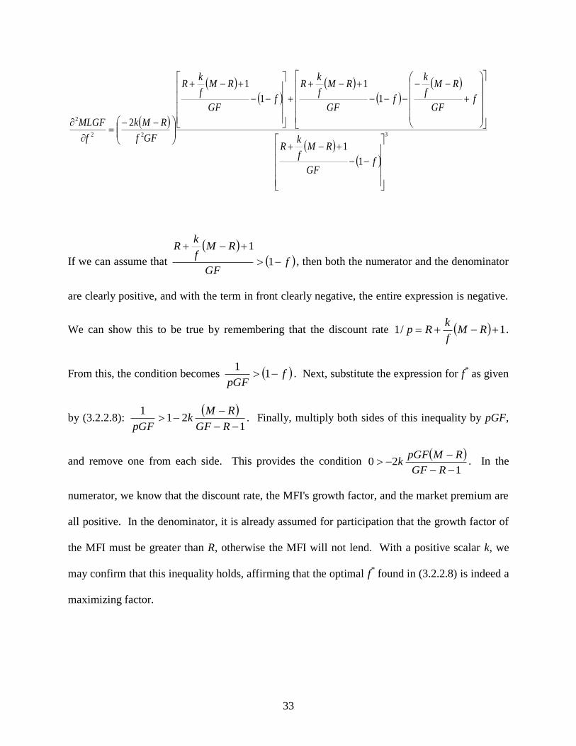
If we can assume that
f
GF
RMf
kR
1
1
, then both the numerator and the denominator
are clearly positive, and with the term in front clearly negative, the entire expression is negative.
We can show this to be true by remembering that the discount rate 1/1 RMf
kRp .
From this, the condition becomes fpGF
11
. Next, substitute the expression for f* as given
by (3.2.2.8):
121
1
RGF
RMk
pGF. Finally, multiply both sides of this inequality by pGF,
and remove one from each side. This provides the condition
120
RGF
RMpGFk . In the
numerator, we know that the discount rate, the MFI's growth factor, and the market premium are
all positive. In the denominator, it is already assumed for participation that the growth factor of
the MFI must be greater than R, otherwise the MFI will not lend. With a positive scalar k, we
may confirm that this inequality holds, affirming that the optimal f* found in (3.2.2.8) is indeed a
maximizing factor.
34
A Note on Infinite Leverage
The modeling of the CMC thus far has been constructed under the assumption that the leverage
provided by the CMC is finite. However, this is not strictly the case. Note from (3.2.2.1) that
the denominator may be zero when fp
GF
1
1. A growth factor greater than this value will
cause the MLGF to be negative. To see this intuitively, consider an MFI with great success in
lending, earning an abnormally high growth factor. If fp
GF
1
1, the MFI will be able to
sell originated loans to the CMC, receiving fGFp 1 in cash. This amount would be greater
than the cash used to originate the loans, so the MFI would be able to increase its intraperiod
cash balance with each round of sales to the CMC. As this would present large firm-specific risk
to the CMC, we may simply assume that the CMC sets a maximum MLGF for each MFI in a
given year. A limit will be chosen in the empirical section.
Summary of Theory
The combination of origination costs with downward sloping demand allows for an optimal
interest rate for the MFI that is not a maximum nor a minimum. Profit maximization demands
that the MFI select a rate that balances the opposing forces of costs and revenue generation,
leading to an outcome similar to that of the credit rationing literature. With this maximization in
place, a nonprofit Central Microcredit Clearinghouse has been shown to potentially enhance MFI
returns, and concomitantly loan balances offered to the poor, with repeated intraperiod purchases
of loan originations.
It has been shown that the CMC may choose an optimal discount rate for asset purchases from

35
the MFI, as well as a ratio of which the purchase price is paid for with securities instead of cash.
The discount rate chosen is the highest that allows for an acceptable risk/return profile of the
resulting CMC security, so that investors are minimally satisfied. The securities purchase ratio is
selected with consideration of the tradeoff between leveraging the MFI's portfolio and limiting
risk. This assumption connects the discount rate and the securities purchase ratio, so that an
unconstrained optimization can be completed with consideration of a single variable.
While it is possible that an MFI may be able to infinitely leverage its portfolio within the
confines of the model, this shortfall can clearly be addressed in practice. If the growth factor of
the MFI is truly large enough to allow for this possibility, and is also sustainable over several
rounds of intraperiod growth, and is not contained by risk levels, then it would eventually be
contained by market saturation, which falls outside of the model.
1.3.3 Solutions Offered by the CMC to Direct Securitization Challenges
In this final section of the introduction of the Central Microcredit Clearinghouse, I will revisit
each of the challenges identified as threats to direct securitization, and show how they are
addressed by the CMC's near-direct securitization innovation. This is a qualitative discussion of
factors leading to the original market failure of microloan securitization, now with an eye on the
CMC as modeled in section 3.2.
The Legal and Regulatory Environment, Macro Policy, and Currency Risk
An investor looking for the chance to assist impoverished citizens of south Asia while making a
fair risk adjusted return would not likely want to assume the risk associated with purchasing
36
claims on microloans in Afghanistan, for example. Most investors are unfamiliar with foreign
law, and want a simple way to invest with some basic level of security. The CMC of a region
such as south Asia would choose to locate in a country with the most favorable regulatory
environment, and the most stable and popular currency for ease of hedging the portfolio to it.
While country risk, political risks, currency risks, policy risks, etc. all remain for a direct
investor, a CMCU would minimize these risks by allowing foreign investors to purchase
CMCUs, and then have the option to hedge their domestic currency.
Donated Funds
Donors will need a new focus. Donations for direct MFI funding will only serve to crowd out
market activity, and retard the growth of the sector. Subsidized microlending should give way to
commercial microlending. The CMC would provide donors with an option that makes their gift
much more powerful than one offered to an MFI. A gift to the CMC for the microloan purchase
and securitization program, much like an investment dollar, would translate directly into an
additional loan, but with the security of knowing that the micro lender is serving its clientele in a
way consistent with the donor's social objectives, and in the most effective and sustainable way.
Even though this would be a popular and dominant portion of the CMC's activities, most donors
would choose to give to other programs within the CMC. Education initiatives, geographic
expansion efforts, micro-borrower advocacy programs, and entrepreneurial guidance efforts are
all potential activities for a CMC. These various programs would present benefactors with a
more effective use of donor dollars than direct lending; they could target special initiatives of
choice under the umbrella of the CMC.

37
Extremely Short-Term Loans
This presents significant problems for any direct securitization. Loan packages would need to be
created so often, that securitization would be very costly on an annualized basis, compared to
other types of securitizations. However, the ongoing creation of CMCUs negate the importance
of average loan term. As new loans come into the pool, and old loans are paid, (or fall into
default), the loan acquisition formula is updated to ensure that the CMCU value is relatively
stable.
Lack of Financial Sophistication in Small MFIs
Smaller MFIs do not possess the expertise in myriad areas necessary for successful loan
securitizations. The presence of the CMC would allow the smallest MFI to securitize their loan
portfolio into CMCUs with minimal training and an internet connection. An online portal for
CMC loan acquisitions would be made simple for the microlender, offering a rate to each lender
based on the criteria discussed above, and in any regional language that is required.
Moral Hazard
The presence of the moral hazard problem is one of the main reasons that direct securitizations
are not expected to ever play a large role in MFI financing. It does indeed appear to be the
Achilles' heel of traditional securitization of microloans. The CMC battles this problem in
multiple ways. First, MFIs will initially be permitted to sell only a portion of their portfolio to
the CMC, receiving a combination of fraction 1-f in cash and f in CMCUs. Third, the value that
the MFI receives in each securitization will be directly linked to past performance of loans,
38
encouraging the close contact and utilization of social pressures that have made microlending
success stories in recent decades.
1.4 Numerical Simulation of a South Asia CMC
In order to better demonstrate the possibilities that exist, this section presents a pseudo-
hypothetical simulation of MFI activity, using data available on actual MFIs operating in South
Asia, for the ten-year period of 2001-2010. Following a brief analysis of the growth of
microlending in South Asia during this decade, I will introduce the South Asia CMC (SACMC),
and run a comparative simulation of what may have transpired during the same time given the
existence of a regional CMC.
1.4.1.1 Data
The Microfinance Information eXchange (MIX) Market collects and processes annual data
submitted by roughly 2,000 microfinance institutions around the world, representing over 90
million borrowers. Information is submitted by representatives of MFIs, or obtained from
external audits, financial statements, management reports, and other sources. All data are
converted from local currencies into USD using an average conversion rate for the period under
survey. Some reporting periods are more or less than a full year; in these cases, data are
annualized using an "annualization factor" calculated based on the number of days in the given
reporting period.
A full set of MIX Market data is available for download at www.mixmarket.org. The dataset is
updated periodically with new rounds of quarterly (for most recent) and annual data. The earliest
39
records date to 1995, with a relatively small amount of data available before 2000. Each MFI is
awarded a diamond rating from 1 to 5, based on its perceived level of data disclosure and
transparency. Diamond ratings of 4 or 5 diamonds indicate that data was submitted, and at least
an external audit was performed. The majority of MFIs in the MIX Market database have a
rating of at least 4 diamonds. Data available from MFIs include the name and location, legal
status, and periodic information about total assets, gross loan portfolio, equity, deposits, various
calculated financial ratios and averages, return, financial expense, numbers of borrowers, and
personnel. Nearly 11,000 records of annual data are available in the full download, offering data
on more than 1,900 microfinance institutions. These institutions are broken down into 6 regions
around the world, covering 116 countries.
For purposes of this simulation, only data from South Asia was retained, and only for years
2001-2010. Some data records are quarterly data provided for years 2010 and 2011, in addition
to 2010 annual data. The quarterly records were deleted, and only the annual records were
retained. Some annual records were deleted for missing both asset and return data. Debt was
calculated from equity and the debt to equity ratios provided. Net income was calculated using
the average ROA and ROE ratios provided. Net income was then divided by beginning of period
assets to serve as a proxy for the MFIs growth factor in a given year.
To err on the side of conservative in the comparative simulation, records with missing return data
that were retained were given an estimated growth factor of one, sufficient to negate CMC
activity for the following year, given that it was also assumed to not have CMC activity
associated with it in the current year. If so, this would provide distortion to the results, and the
record was deleted. Any record with missing return data for a year within a series of operational

40
years with CMC activity had returns estimated based on surrounding ROA data, since deletion of
these records would be more disruptive to the simulation. This adjustment was made for just 5
records.19
Assets were estimated for 2 records.20
Two MFIs were removed from the dataset for
having only 2001 balance sheet data, and no activity.21
1.4.1.2 Microfinance Institutions in South Asia
The South Asian region per Mix Market demarcation includes the countries of Afghanistan,
Bangladesh, Bhutan, India, Nepal, Pakistan, and Sri Lanka. Some basic information for reported
activity and financial position is shown in Table 4.1.2.1, along with indicators of income and
poverty which are provided by the World Bank.
Country # of
MFIs
Gross Loan
Portfolio
Number
of Active
Borrowers
Average
Loan
Size
GNI
Per-
capita,
current
$
Poverty
Headcount
Ratio
# of 4-5
Diamond
MFIs
Afghanistan 12 $ 127,276,014 268,431 $474 $410 36.0%* 6
Bangladesh 29 $2,633,780,287 22,656,208 $116 $700 31.5% 11
Bhutan 1 $ 94,992,904 24,476 $3,244 $1,870 23.2%* 0
India 94 $5,251,114,050 31,794,850 $165 $1,270 37.2%* 47
Nepal 28 $ 153,710,606 725,187 $212 $490 25.2%* 19
Pakistan 27 $ 261,192,518 1,883,013 $139 $1,050 22.3%* 16
Sri Lanka 18 $ 526,524,296 1,334,744 $394 $2,240 8.9% 6
Table 4.1.2.122
*indicates that data is for a year close to 2010
19
This was done for VYCCU in Nepal for 2006, BMSCCSL in Nepal for 2006, BASTOB in
Bangladesh for 2008, CSS in Bangladesh for 2007, and Shakti in Bangladesh for 2010. 20
This was done for WDFH in Sri Lanka for 2005 and 2006, using asset/gross loan portfolio
ratios and the surrounding asset balances for 2004 and 2007. Growth factors of one were
assumed in these years. 21
These were CCODER in Nepal and NLCL in Pakistan. 22
Data is from the Mix Market (www.mixmarket.org), and the World Bank (data.worldbank.org)
41
There are several initial items of note. First, while there are 209 MFIs operating in the 7-nation
region designated by the MIX as South Asia, only 105 of these possess the necessary history and
transparency to earn a 4 or 5 diamond Mix Market rating. The SACMC could start securitizing
loans from 6 of the 7 countries, but efforts in Bhutan would initially be limited to assisting MFIs
with reporting and transparency issues so that they can achieve membership status. For this
reason, Bhutan will not be included in the remaining analyses.
The MFIs reporting data in south Asia combine to a gross loan portfolio as of 2010 of $9 billion.
Dividing the gross loan portfolio by the number of active borrowers in each nation provides an
average loan size for the reported loan activity in each country. When we compare this with the
GNI per-capita, we find that the average borrower of Afghanistan's MFIs actually borrows over
100% of their per-capita GNI. For the other five countries, the average loan size ranges from
13% to 43% of per-capita GNI, with an overall weighted mean of 16.3%23
. These numbers
indicate that an average micro-borrower in this region receives about 2 months of the nation-
wide average income for a typical microloan. The final column counts only the four and five
diamond rated MFIs. This reduces the gross loan portfolio under consideration from $9 billion
to $7.7 billion, but removes half of the original 209 MFIs represented. This relatively small
reduction in total assets demonstrates that the largest MFIs are also those with sufficient history
and transparency to earn those higher diamond ratings.
The headcount ratio is captured here only as an input to a rough indication of market penetration.
Assume that just half of all impoverished persons (found as the product of each nation's
23
With Afghanistan removed, and ignoring Bhutan, Nepal is the new outlier, with borrowers
having an average of 43.3% GNI per capita. The other 4 are all between 13.0% and 17.6%.
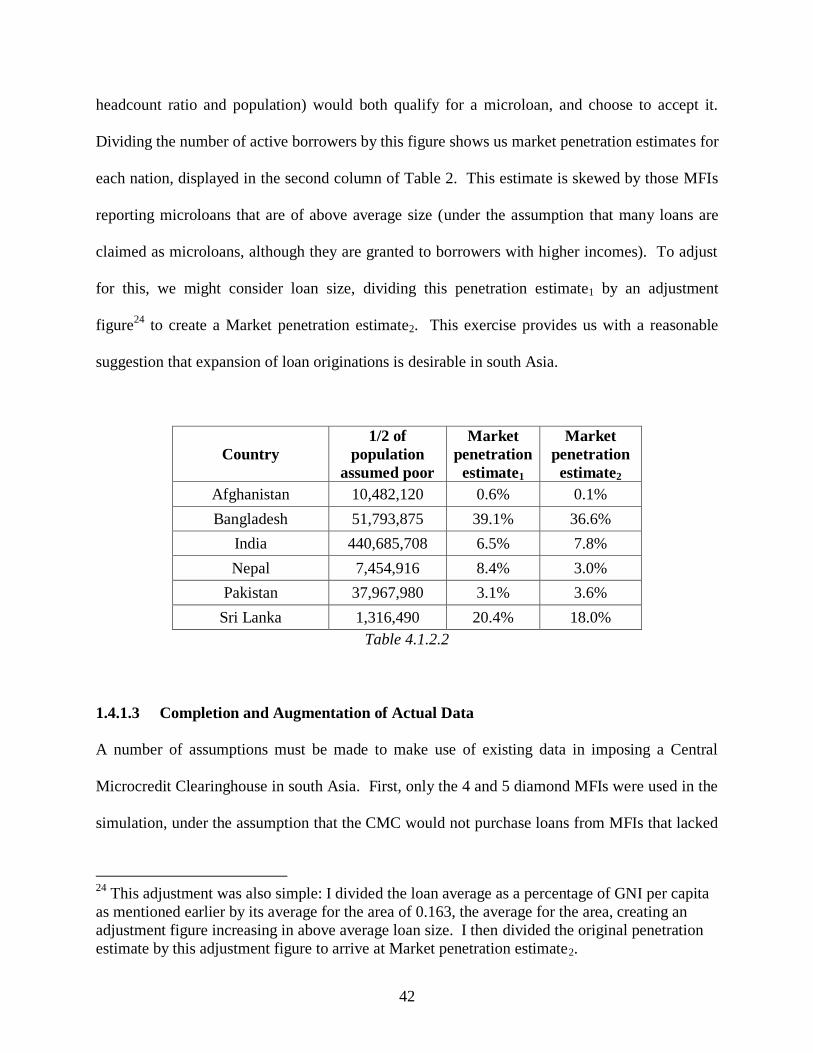
42
headcount ratio and population) would both qualify for a microloan, and choose to accept it.
Dividing the number of active borrowers by this figure shows us market penetration estimates for
each nation, displayed in the second column of Table 2. This estimate is skewed by those MFIs
reporting microloans that are of above average size (under the assumption that many loans are
claimed as microloans, although they are granted to borrowers with higher incomes). To adjust
for this, we might consider loan size, dividing this penetration estimate1 by an adjustment
figure24
to create a Market penetration estimate2. This exercise provides us with a reasonable
suggestion that expansion of loan originations is desirable in south Asia.
Country
1/2 of
population
assumed poor
Market
penetration
estimate1
Market
penetration
estimate2
Afghanistan 10,482,120 0.6% 0.1%
Bangladesh 51,793,875 39.1% 36.6%
India 440,685,708 6.5% 7.8%
Nepal 7,454,916 8.4% 3.0%
Pakistan 37,967,980 3.1% 3.6%
Sri Lanka 1,316,490 20.4% 18.0%
Table 4.1.2.2
1.4.1.3 Completion and Augmentation of Actual Data
A number of assumptions must be made to make use of existing data in imposing a Central
Microcredit Clearinghouse in south Asia. First, only the 4 and 5 diamond MFIs were used in the
simulation, under the assumption that the CMC would not purchase loans from MFIs that lacked
24
This adjustment was also simple: I divided the loan average as a percentage of GNI per capita
as mentioned earlier by its average for the area of 0.163, the average for the area, creating an
adjustment figure increasing in above average loan size. I then divided the original penetration
estimate by this adjustment figure to arrive at Market penetration estimate2.
43
this level of transparency. Also, it is assumed that if an MFI qualifies for CMC affiliation, and
purchase of receivables, the MFI will sell all receivables to the CMC when p > pmin, and use all
cash received to originate more loans for sale, continuing this intraperiod loop to take advantage
of the multiplier effect, reaching the Maximum Leveraged Growth Factor (MLGF) as modeled.
From here, the growth factor (GF) and MLGF for each MFI shall be indexed by m = 1...M, and
time shall be indexed t = 1...T, allowing for a matrix of empirical growth factors represented by
GFmt. Recall from the note at the end of section 3.2, that when fp
GFmt
1
1, 0mtMLGF ,
which indicates an infinite multiplier. There are instances in the data when the proxied mtGF
exceeds this "limit," which would allow the MFI to originate loans, sell fraction f at the
discounted rate to the CMC, and still receive more cash back from the sale than it had in assets at
the beginning of the period. To address this, some maximum was needed, and that maximum was
set rather arbitrarily at 3.25
The procedure for simulating MFI data begins with its first financial position of record. In its
second financial position of record, income statement activity is reported for that year. Two
years of financial position are then the minimum for provision of a growth factor estimate, from
which subsequent CMC eligibility can be determined. The third year of record provides the third
financial position, and the second set of return data. This is the MFI's first possible chance to
enhance their activity in partnership with the CMC. For each year of record, if p > pmin for the
25
In an effort to leave the simulation free from constraints as much as possible, 3 was chosen as
a rather high limit. Note that this means an MFI would be able to use CMC cash to triple its size
in a given year. Also, of the 686 MLGFs estimated in the dataset, only 11 reached this
maximum value, and in only 6 of those instances was the MFI eligible for CMC funding in that
period, and so was able to triple its simulated value.

44
MFI in the prior year, then the MFI will sell all loans to the CMC in the current year. Since 10
years of data were collected and used for this simulation, each MFI retained in the dataset has 1-
9 years of financial activity reported, and 0-8 years of financial activity augmented with
receivable sales to the CMC. Table 4.1.3.1 provides a snapshot of what data is available from
each year.
A total of 133 MFIs are included in the dataset. The first 3 columns of Table 4.1.3.1 demonstrate
a considerable amount of turnover in reporting (and potentially, operation) of these
organizations. Only 12 MFIs reported data for all 10 years under observation. All MFIs in the
dataset reported a continuous and uninterrupted set of years. A few items had to be imputed, as
reported in the previous section.
The summation of balance sheet items grew at roughly the same pace from year to year. On
average, MFIs in this region expanded with largely the same debt/asset and debt/equity ratios.
Assets grew at an average rate of 37.6% over this time period, debt at an average rate of 38.8%,
and equity at an average rate of 35.0%. Meanwhile, the balance of outstanding loans grew at an
average rate of 38.8%, maintaining a relatively consistent ratio of loans to both assets and debt.
This indicates that perhaps MFIs choose to maintain a stable debt ratio, and that perhaps an
expansion of assets via a CMC receivables purchase program would precede an expansion of
debt, furthering asset expansion even more. However, this is not an assumption made in the
simulation. Actual debt values are assumed in the simulation to be unchanged. Additional
lending made possible by the CMC is assumed to expand the asset balance of the MFI, and also
the equity of the MFI in the same amount.
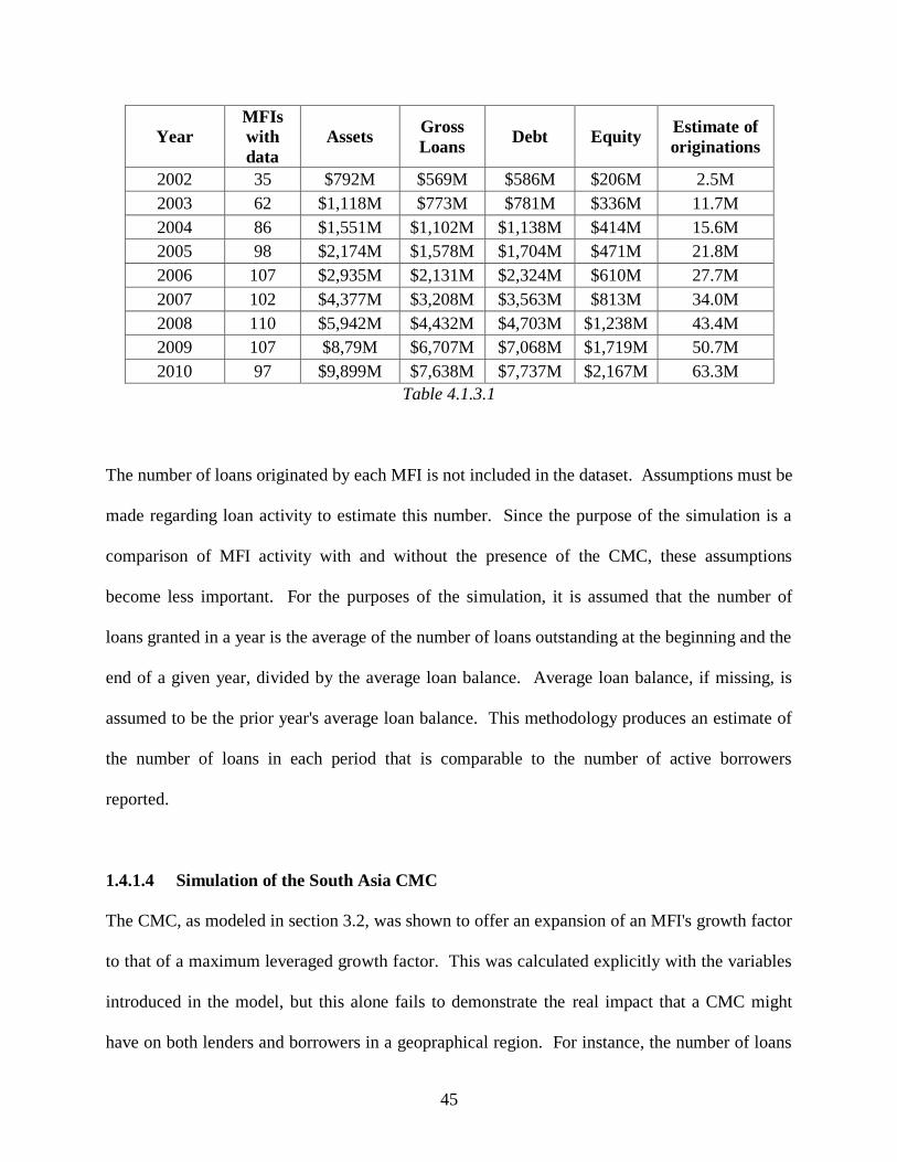
45
Year
MFIs
with
data
Assets Gross
Loans Debt Equity
Estimate of
originations
2002 35 $792M $569M $586M $206M 2.5M
2003 62 $1,118M $773M $781M $336M 11.7M
2004 86 $1,551M $1,102M $1,138M $414M 15.6M
2005 98 $2,174M $1,578M $1,704M $471M 21.8M
2006 107 $2,935M $2,131M $2,324M $610M 27.7M
2007 102 $4,377M $3,208M $3,563M $813M 34.0M
2008 110 $5,942M $4,432M $4,703M $1,238M 43.4M
2009 107 $8,79M $6,707M $7,068M $1,719M 50.7M
2010 97 $9,899M $7,638M $7,737M $2,167M 63.3M
Table 4.1.3.1
The number of loans originated by each MFI is not included in the dataset. Assumptions must be
made regarding loan activity to estimate this number. Since the purpose of the simulation is a
comparison of MFI activity with and without the presence of the CMC, these assumptions
become less important. For the purposes of the simulation, it is assumed that the number of
loans granted in a year is the average of the number of loans outstanding at the beginning and the
end of a given year, divided by the average loan balance. Average loan balance, if missing, is
assumed to be the prior year's average loan balance. This methodology produces an estimate of
the number of loans in each period that is comparable to the number of active borrowers
reported.
1.4.1.4 Simulation of the South Asia CMC
The CMC, as modeled in section 3.2, was shown to offer an expansion of an MFI's growth factor
to that of a maximum leveraged growth factor. This was calculated explicitly with the variables
introduced in the model, but this alone fails to demonstrate the real impact that a CMC might
have on both lenders and borrowers in a geopraphical region. For instance, the number of loans

46
and the loan amounts both with and without CMC inclusion are not calculated in the model, as
many things such as loan demand, loan tenor, optimal interest rates, etc. would all need to be
estimated.
By reaching to actual empirical data, these values can be obtained by calibrating the model, and
estimating several items of interest to policymakers, asking questions such as: How many extra
borrowers would be served? What would the differential effects be across the nations? Would
market saturation be reached anywhere? How would the expansion of investor dollars compare
to the total asset balances already in place in microfinance institutions? Through this final effort,
some estimates may be provided for these questions.
To begin a simulation of the CMC model in South Asia, a growth factor for each MFI for each
year of observation was needed. Such a growth factor could be estimated as modeled, using a
cost per loan, interest income, etc. However, this would ignore idiosyncratic and systematic
risks that affected microlending in this region over the decade. The growth factor, under the
assumption that cash is inelastically supplied to the microloan market by each MFI in each
period, serves as a measure of growth for the organization given beginning period assets. For
this reason, the return on assets (ROA) measure provided was used to calculate net income for
each period, and this was used in conjunction with the beginning period asset balance to create a
proxy for the growth factor in each of the 10 years, across each of the 133 MFIs.
With the array mtGF , the array mtMLGF can be calculated, using (3.2.2.1), with the additional
parameters for the fraction of loan value purchased for noncash consideration f and the gross
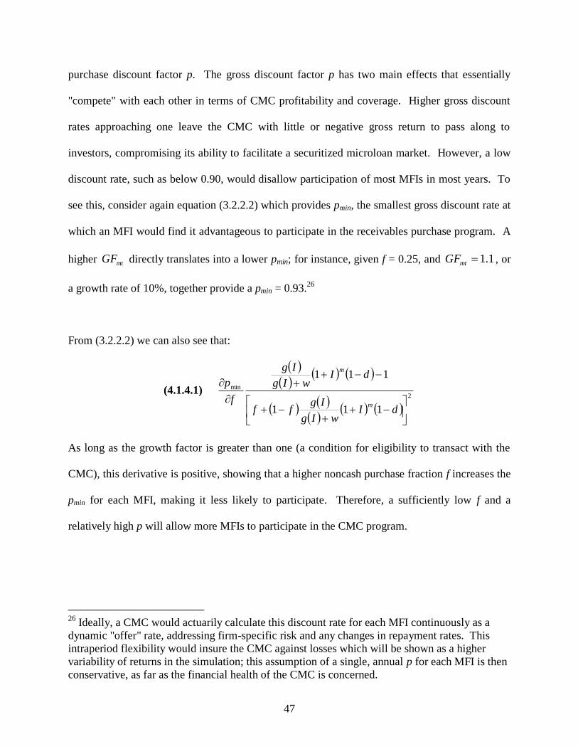
47
purchase discount factor p. The gross discount factor p has two main effects that essentially
"compete" with each other in terms of CMC profitability and coverage. Higher gross discount
rates approaching one leave the CMC with little or negative gross return to pass along to
investors, compromising its ability to facilitate a securitized microloan market. However, a low
discount rate, such as below 0.90, would disallow participation of most MFIs in most years. To
see this, consider again equation (3.2.2.2) which provides pmin, the smallest gross discount rate at
which an MFI would find it advantageous to participate in the receivables purchase program. A
higher mtGF directly translates into a lower pmin; for instance, given f = 0.25, and 1.1mtGF , or
a growth rate of 10%, together provide a pmin = 0.93.26
From (3.2.2.2) we can also see that:
(4.1.4.1)
2
min
111
111
dIwIg
Igff
dIwIg
Ig
f
p
m
m
As long as the growth factor is greater than one (a condition for eligibility to transact with the
CMC), this derivative is positive, showing that a higher noncash purchase fraction f increases the
pmin for each MFI, making it less likely to participate. Therefore, a sufficiently low f and a
relatively high p will allow more MFIs to participate in the CMC program.
26
Ideally, a CMC would actuarily calculate this discount rate for each MFI continuously as a
dynamic "offer" rate, addressing firm-specific risk and any changes in repayment rates. This
intraperiod flexibility would insure the CMC against losses which will be shown as a higher
variability of returns in the simulation; this assumption of a single, annual p for each MFI is then
conservative, as far as the financial health of the CMC is concerned.
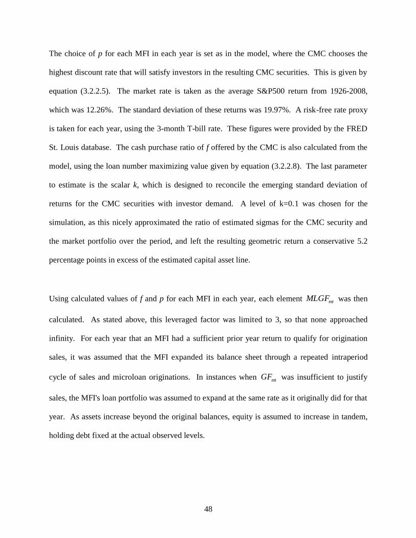
48
The choice of p for each MFI in each year is set as in the model, where the CMC chooses the
highest discount rate that will satisfy investors in the resulting CMC securities. This is given by
equation (3.2.2.5). The market rate is taken as the average S&P500 return from 1926-2008,
which was 12.26%. The standard deviation of these returns was 19.97%. A risk-free rate proxy
is taken for each year, using the 3-month T-bill rate. These figures were provided by the FRED
St. Louis database. The cash purchase ratio of f offered by the CMC is also calculated from the
model, using the loan number maximizing value given by equation (3.2.2.8). The last parameter
to estimate is the scalar k, which is designed to reconcile the emerging standard deviation of
returns for the CMC securities with investor demand. A level of k=0.1 was chosen for the
simulation, as this nicely approximated the ratio of estimated sigmas for the CMC security and
the market portfolio over the period, and left the resulting geometric return a conservative 5.2
percentage points in excess of the estimated capital asset line.
Using calculated values of f and p for each MFI in each year, each element mtMLGF was then
calculated. As stated above, this leveraged factor was limited to 3, so that none approached
infinity. For each year that an MFI had a sufficient prior year return to qualify for origination
sales, it was assumed that the MFI expanded its balance sheet through a repeated intraperiod
cycle of sales and microloan originations. In instances when mtGF was insufficient to justify
sales, the MFI's loan portfolio was assumed to expand at the same rate as it originally did for that
year. As assets increase beyond the original balances, equity is assumed to increase in tandem,
holding debt fixed at the actual observed levels.
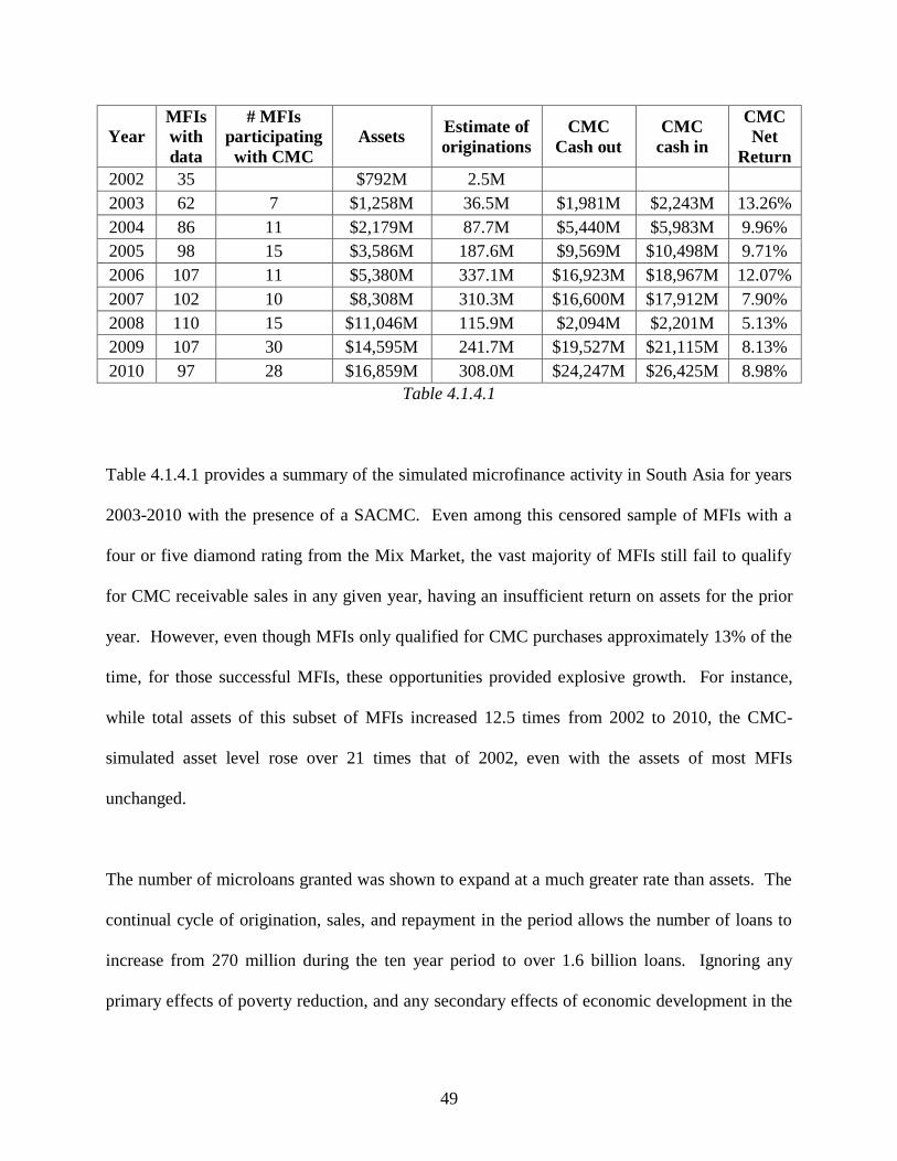
49
Year
MFIs
with
data
# MFIs
participating
with CMC
Assets Estimate of
originations
CMC
Cash out
CMC
cash in
CMC
Net
Return
2002 35 $792M 2.5M
2003 62 7 $1,258M 36.5M $1,981M $2,243M 13.26%
2004 86 11 $2,179M 87.7M $5,440M $5,983M 9.96%
2005 98 15 $3,586M 187.6M $9,569M $10,498M 9.71%
2006 107 11 $5,380M 337.1M $16,923M $18,967M 12.07%
2007 102 10 $8,308M 310.3M $16,600M $17,912M 7.90%
2008 110 15 $11,046M 115.9M $2,094M $2,201M 5.13%
2009 107 30 $14,595M 241.7M $19,527M $21,115M 8.13%
2010 97 28 $16,859M 308.0M $24,247M $26,425M 8.98%
Table 4.1.4.1
Table 4.1.4.1 provides a summary of the simulated microfinance activity in South Asia for years
2003-2010 with the presence of a SACMC. Even among this censored sample of MFIs with a
four or five diamond rating from the Mix Market, the vast majority of MFIs still fail to qualify
for CMC receivable sales in any given year, having an insufficient return on assets for the prior
year. However, even though MFIs only qualified for CMC purchases approximately 13% of the
time, for those successful MFIs, these opportunities provided explosive growth. For instance,
while total assets of this subset of MFIs increased 12.5 times from 2002 to 2010, the CMC-
simulated asset level rose over 21 times that of 2002, even with the assets of most MFIs
unchanged.
The number of microloans granted was shown to expand at a much greater rate than assets. The
continual cycle of origination, sales, and repayment in the period allows the number of loans to
increase from 270 million during the ten year period to over 1.6 billion loans. Ignoring any
primary effects of poverty reduction, and any secondary effects of economic development in the
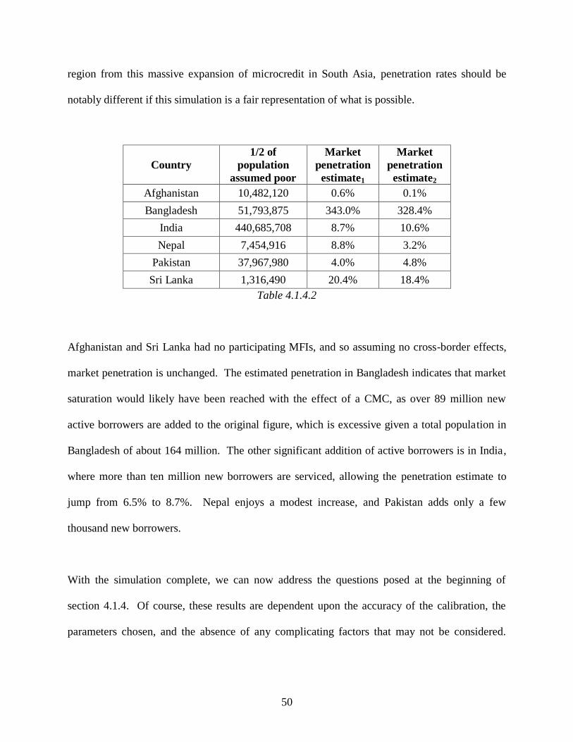
50
region from this massive expansion of microcredit in South Asia, penetration rates should be
notably different if this simulation is a fair representation of what is possible.
Country
1/2 of
population
assumed poor
Market
penetration
estimate1
Market
penetration
estimate2
Afghanistan 10,482,120 0.6% 0.1%
Bangladesh 51,793,875 343.0% 328.4%
India 440,685,708 8.7% 10.6%
Nepal 7,454,916 8.8% 3.2%
Pakistan 37,967,980 4.0% 4.8%
Sri Lanka 1,316,490 20.4% 18.4%
Table 4.1.4.2
Afghanistan and Sri Lanka had no participating MFIs, and so assuming no cross-border effects,
market penetration is unchanged. The estimated penetration in Bangladesh indicates that market
saturation would likely have been reached with the effect of a CMC, as over 89 million new
active borrowers are added to the original figure, which is excessive given a total population in
Bangladesh of about 164 million. The other significant addition of active borrowers is in India,
where more than ten million new borrowers are serviced, allowing the penetration estimate to
jump from 6.5% to 8.7%. Nepal enjoys a modest increase, and Pakistan adds only a few
thousand new borrowers.
With the simulation complete, we can now address the questions posed at the beginning of
section 4.1.4. Of course, these results are dependent upon the accuracy of the calibration, the
parameters chosen, and the absence of any complicating factors that may not be considered.
51
However, to the extent that these factors are minimal, some summary results may be offered to
these questions:
How many extra borrowers would be served? By comparing tables 4.1.3.1 and 4.1.4.1, the
estimated number of originations is extraordinary. Where the microcredit market in South Asia
grew from an estimated 2.5 million loans to 63 million loans over the decade, expansion of this
activity by a SACMC would have possibly allowed this level to be reached in just two years
rather than eight, achieving six times the number of loans over the period.
What would the differential effects be across the nations? Would market saturation be reached
anywhere? We can see that Bangladesh would have reached a point of market saturation, while
Afghanistan and Sri Lanka would be unaffected, due to the underdevelopment of MFIs there.
This is a consistent outcome with the main focus of the CMC, which is to accelerate the
progression of microcredit markets, rather than to offer nascent growth in regions where there is
little or none. Again, the innovations in microlending are expected to come from local lenders.
Therefore, the CMC is not in a position to guarantee expansion of microcredit everywhere;
rather, it serves to reward successful efforts where they arise.
How would the expansion of investor dollars compare to the total asset balances already in place
in microfinance institutions? Assets of South Asian MFIs grew to $10 billion by 2010. With the
CMC, this would have been roughly $16 billion. This is a rather modest increase in percentage
terms, but as discussed, the increase in origination activity would have been much larger. The
investor dollars committed to lending activity would have reached $26 billion in 2010. These

52
numbers suggest that new dollars introduced to the market via CMC securitizations may be more
efficient in achieving market completion than those placed on the balance sheets of MFIs.
Where a new loan is originated for every $156 of assets with an MFI in South Asia, a loan can be
generated with just $99 of investor purchases of CMC securities.
1.4.1.5 Viability of CMC Securities
The parameterization of the simulation suggested that a CMC security over this decade would
have provided a geometric return of 9.37% to investors, with a standard deviation of returns of
just 2.36%. Again, this simulation allowed the CMC just one level of f and p for the year,
regardless of the continual performance of loans and loan payment remittance.
Expected CMC Security Returns as a function of k
Figure 4.1.5.1

53
Clearly, if investors were willing to place a social premium on CMC security returns, it may be
feasible for the CMC to increase its discount rate to encourage more participation. Such a
marked differential in performance between participating and nonparticipating MFIs perhaps
would, in the presence of the CMC, encourage best practices and adoption of efficiencies among
smaller organizations that may further spur growth of the microfinance industry.
The behavior of the CMC securities varies significantly with the choice of the parameter k. At
lower levels, the assumed variance in the CMC security is very low, allowing for a lower optimal
choice of f*. However, returns are lower, given that this makes origination sales viable for a
greater subset of MFIs, adding lower performance loans to the average.
It is also important to note that the number of new loans generated varies widely with the choice
of the k parameter. Although it appears that a higher estimate is more beneficial to the CMC in
achieving its goal, this is not the case. Figure 4.1.5.1 shows satisfaction of the constraint. But
the goal of increased loan takeup falls rapidly at higher levels of k. In fact, recall that the CMC's
simulated activity provided an additional 1.3 billion loans to the microcredit markets in southeast
Asia during the ten year period, given the choice of k = 0.1. If this parameter was k = 0.12
instead, the estimated number of new loans would be less than half of this figure. This
demonstrates, perhaps most clearly, the importance of organizing microloans into a diversified,
well-monitored, and low risk security.
54
1.5 Conclusion
As we start to seriously consider the viability of an organization such as the South Asia Central
Microcredit Clearinghouse, many aspects of its size, structure, form, management, missions, and
scope should be the subject of discussion. It's organization as a nonprofit arose from a logical
analysis of the challenges confronting the potential of a microloan securitization market, and
future work will determine if this is indeed the correct organizational form for a CMC.
A legal analysis is required. Only an introduction to this important contribution is provided here,
but a detailed legal opinion would contribute a great deal to this initial effort. The development
of a tailored CMC software system would show operational viability. Leading MFIs from the
region could provide insight as to whether this effort would be a welcome addition to their
financing options. Investors would need to be convinced of the strength and backing of a CMC
security.
While a large MFI might be the logical point for the spawning of a prototype CMC,
independence is arguably of importance. It would likely be most beneficial to the sustainability
of the program to have its origination minimally connected with a specific MFI, but rather a
project of an NGO with a mission of poverty alleviation that is itself not a direct lender. Starting
with one CMC, perhaps in South Asia, would provide a springboard to other regional CMCs
beginning operation in other parts of the world as microfinance services continue to develop.
A CMC would not contest the desire of MiCDOs. Diversified lending to MFIs has served as a
useful bridge between some investors and microlenders. While MiCDOs are arguably the best
55
way of funding MFIs within the framework of a traditional financial tool set, I have shown here
that a near-direct securitization of microloans is possible, with the help of a regional nonprofit
organization to serve as a Central Microcredit Clearinghouse.
With the aid of a CMC, regional MFIs could have greater access to investor funds by allowing
them the "pure play" on the underlying asset, which is attractive to many foreign investors.
Local MFIs would themselves hold some securities as partners of the securitization program.
Loans to impoverished citizens would be expanded. Profits of MFIs would rise. The existence
of a CMC would allow the securitization of microloans to be a sustainable and socially beneficial
reality. The organization at the center of these solutions may indeed usher in a new chapter in
microcredit capital market access. If successful, perhaps we could witness this industry moving
into a competitive equilibrium in years, rather than decades.

56
Chapter 1 Appendix A
Cash at discrete times
The equation (3.2.1.1) of
Ig
WOId
m
IORCC t
t
mtk
m
ktt 111
11
1 assumes that
cash is zero. That is, imagine that the MFI gets all payments on the first of every month exactly
at noon, then immediately re-loans that money to new borrowers waiting at the door. The instant
that time t-1 becomes time t is at noon on the first. At time t, the money has come in, gone out,
and cash is zero again. This is why there's no return on past cash.
Alternatively, we could reformulate the equation so that time t is exactly at noon on the first of
that month, in that split second when cash is moving from the inbox to the outbox. In this case,
the equation would be
1
11 11
11t
mtk
m
kttt Idm
IOR
Ig
WOCC .
Now, cash is a positive balance each period; payments have just come in, they are about to go
out, but haven't quite yet. The last origination was now last period, so the final term is indexed
as t-1. Also, the cash return is not multiplied by t-1 cash, but by t-1 cash that was unused as
originations and related fees.
Given these options, I opted for the former.

57
Chapter 1 Appendix B
Existence of bounded roots for (3.2.1.4)
It is necessary that (3.2.1.4) yield both an Imax and Imin when this inequality holds with equality,
so that an interior maximizing value I* also exists. Here, I show the existence of these two real
values. I have assumed that there is positive demand for funds which is everywhere
differentiable and decreasing in I. Also, there is a positive default rate which is everywhere
differentiable and increasing in I (up to some finite value of I where d(I) = 1, the area beyond
which is trivial). Also, negative interest rates are assumed to not exist. Given these assumptions,
for a given interest rate I, there must exist some value of origination cost w such that
111
IdIwIg
Ig m
This value is found as
111 IdIIgwm
It is possible, if 111 IdIm
, that the value of w that allows this equality is negative.
However, the origination cost w is assumed to be greater than zero. Therefore, given some
functions of g(I) and d(I), it is possible that (3.2.1.4) does not hold. This is simply the condition
when lending is unprofitable, and does not occur. To allow for lending, we allow for the
condition
Id
RI
wIg
Ig m
11
so that lending is profitable for the MFI, and occurs. As w increases, the left hand side is
reduced, and this inequality moves toward equality. There is, therefore, some maximum real
value of origination cost w that makes this equal, such that
58
Id
RI
wIg
Ig m
11
At this level of origination cost, the growth factor is R, and the MFI is indifferent between
microlending and investment in the risk-free asset. However, we can return to (3.2.1.4), taking
the first derivative of the GF with respect to w:
211
wIg
IgIdI
w
GF m
This value is clearly negative, showing that decreasing origination costs allow for a larger
growth factor. Therefore, when origination costs are below the maximum, interest rates may be
lowered. At an interest rate of zero, (3.2.1.4) clearly becomes zero. The intermediate value
theorem therefore provides for the existance of some value Imin that allows (3.2.1.4) to hold with
equality.
Since the default function d(I) = 1 for some finite value of I, this interest rate level also forces the
growth factor to be zero. Once again, the intermediate value theorem dictates that there then
must exist some value Imax for which the growth factor is equal to R. Again, it is not important
that these are the only two roots, but that these roots exist as growth factor minimums. The
assumptions made then allow for the growth factor to be convex and differentiable, creating the
growth factor maximizing interest rate level I* as provided by (3.2.1.8).
59
Chapter 2
Disbursements of ODA:
A Function of the Business Cycle?
Chapter Summary
I analyze Official Development Assistance (ODA) commitment and disbursement activity in
terms of motivation, considering that the difference between bilateral aid commitments and
disbursements may be related to the business cycle of the donor country. A cumulative
commitment variable is calculated for 23 donor countries and 151 recipient nations, over a 41
year period of 1970-2010, as well as the sub-period of 1991-2010. Cyclicality of aid is briefly
analyzed first, with mixed results of procyclicality that depend on the business cycle proxy. The
annual disbursement gap is calculated for each pair for each year, as well as a cumulative
disbursement gap, and these are regressed against multiple cyclicality measures of income and a
set of control variables. It is found in multiple specifications that the cumulative disbursement
gap is generally procyclical, much as aid itself, although the cyclicality of aid depends on the
cyclicality measure. This is confirmed with four extensions designed mainly as robustness
checks.
60
2.1 Introduction
Official Development Assistance (ODA) has been a long-debated subject in terms of both
effectiveness and motivation. Suggested motivations of nations to engage in bilateral foreign aid
are numerous. McKinlay & Little (1977) recognized the main motivations of bilateral foreign
aid as a dichotomy of the desire to truly help a recipient nation, and the goal of imperialism and
donor self-interest, finding some evidence of the latter for some aid during the 1960s. Many
agree that one of the main motivations of aid appears to be the donor's own interest (Berthelemy
& Tichit, 2004; Berthelemy, 2006; Alesina & Dollar, 2000; Nielsen, 2009), including the desire
to strengthen political relationships, trade interests, and influence within the recipient nation
(Maizels & Nissanke, 1984). Additionally, political variables, such as a shift within the donor
nation's conservative regime, is shown to be related to aid flows to poor nations (McGillivray &
Oczkowski, 1992; Tingley, 2010).
It is noted that corruption does not appear to deter aid; also, aid does not appear to deter
corruption (Svensson, 1997; Alesina & Weber, 1999). However, other factors of the recipient
country have been isolated as relating to aid flows, such as population of the recipient country.
Smaller countries are noted for receiving more aid. This is often explained as donors perhaps
feeling a greater effect to their aid; however, this effect is greatly diminished with control
variables for exports and political dummies (Dudley & Montmarquette, 1976).
The timing of aid has been shown to be important in the management of a developing economy.
Unpredictability of aid can cause a recipient nation to remain in a low-level equilibrium trap
(Eifert & Gelb, WP). It has specifically been found to lower investment (Hudson & Mosley,
61
2008). This variability has been found to be procyclical in studies of the relationship between
aid and the business cycle, including commitments (Dabla-Norris, Minoiu, & Zanna 2010).
However, commitments have been noted as somewhat less procyclical (Pallage & Robe, 2001).
Bulíř & Hamann (2008) also point to variability of aid as a culprit in making macroeconomies of
the poorest nations harder to manage, and demonstrate that one driver of this variation is the
difference between aid commitments and disbursements. This difference comes (at least in part)
by the structure of donor governments; the agencies approving aid are often not the same as
those disbursing the aid. It can take several years for a commitment to be disbursed. A
commitment is recorded as disbursed when financial resources are transferred to the recipient, or
in the case of services, when payment is made to the provider of the service (oecd.org).
The difference between commitments and disbursements has been shown to change over time.
Bulíř & Hamann (2008) show, using loan data the World Bank's Global Development Finance
database, that the ratio of loan commitments to disbursements fell throughout the 1980s, for
instance, but then stabilize to about 1.5. Further, the disparity appears greater with regard to the
lowest-income recipients. This gap between promises and action, also known as the
unpredictability of aid, is perhaps not only motivated by bureaucracy, but perhaps also by fiscal
balances, credit stance, and the overall business cycle of the donor nation. These relationships,
and the timing of cumulative differences between foreign aid commitments and disbursements,
are the focus of this paper. Using OECD data on foreign aid grants, loans, and total aid, this
disparity will be analyzed with respect to several relevant variables.

62
Multiple research questions arise as testable assumptions with regard to the behavior of
commitments and disbursements with regard to the business cycle. First, several past studies
have shown aid to be generally procyclical with respect to donor income; will the same be found
in the present dataset? Second, is the simple difference between commitments and
disbursements in a given year correlated with donor income, indicating that a donor's failure to
pay immediately may be related to economic downturn? Third, can we find similar results by
looking at a cumulative measure of foreign aid commitments payable? Finally, are the results we
find robust to varying parameterizations and control variables?
While the analysis of the disbursement gap is atheoretic, this initial analysis assumes that there
may be some function that describes the disbursement gap, such as
drdrd FiscSurpYYCYCCYCfCDG ,,,,
where a cumulative disbursement gap is related to the cyclicality of income for the donor and
recipient, the level of income for the donor and recipient, and the fiscal surplus of the donor
nation. The nature of this work will be exploratory, looking for empirical relationships among
these variables, in multiple measures, that are robust.
The remainder of the paper is organized as follows: Part 2 presents the data which has been
gathered for the present analysis. Part 3 discusses the methods of analysis employed in utilizing
the data to help us answer the research questions presented Part 4 concludes.

63
2.2 Data
Most data was obtained from stats.oecd.org. This website offers data on GDP, ODA
commitments, ODA disbursements, and myriad other data. Data was obtained on annual totals
for 1966-2010 on ODA grant commitments and disbursements, ODA loan commitments and
disbursements, and ODA total commitments and disbursements. These were obtained for each
of 23 Development Assistance Committee (DAC) countries, and 151 recipient nations, classified
by stats.oecd as either Least Developed Countries (LDCs), Low Income Countries (LICs), Low
Middle Income Countries (LMICs), or Upper Middle Income Countries (UMICs). The
measurement chosen for each of these datasets was 2010 constant prices in USD. Full time
employment percentages were also obtained from stats.oecd for each of the 23 DAC nations,
using national definitions of employment, as well as budget surpluses as a percentage of GDP for
these 23 nations. A number of foreign aid components are available for analysis, including six
types of commitments and 22 types of disbursements. Of these, Total Grants, Total Gross
Loans, and Total Net ODA were chosen for analysis. Grant commitments and loan
commitments together comprise 99.6% of total net ODA committed.
Data on national income was obtained from unctadstat.unctad.org, the website of the United
Nations Conference on Trade and Development. This dataset contained annual GDP per capita
figures in 2005 constant prices, in USD. This dataset supplied income figures for both the donor
and recipient nations under analysis.
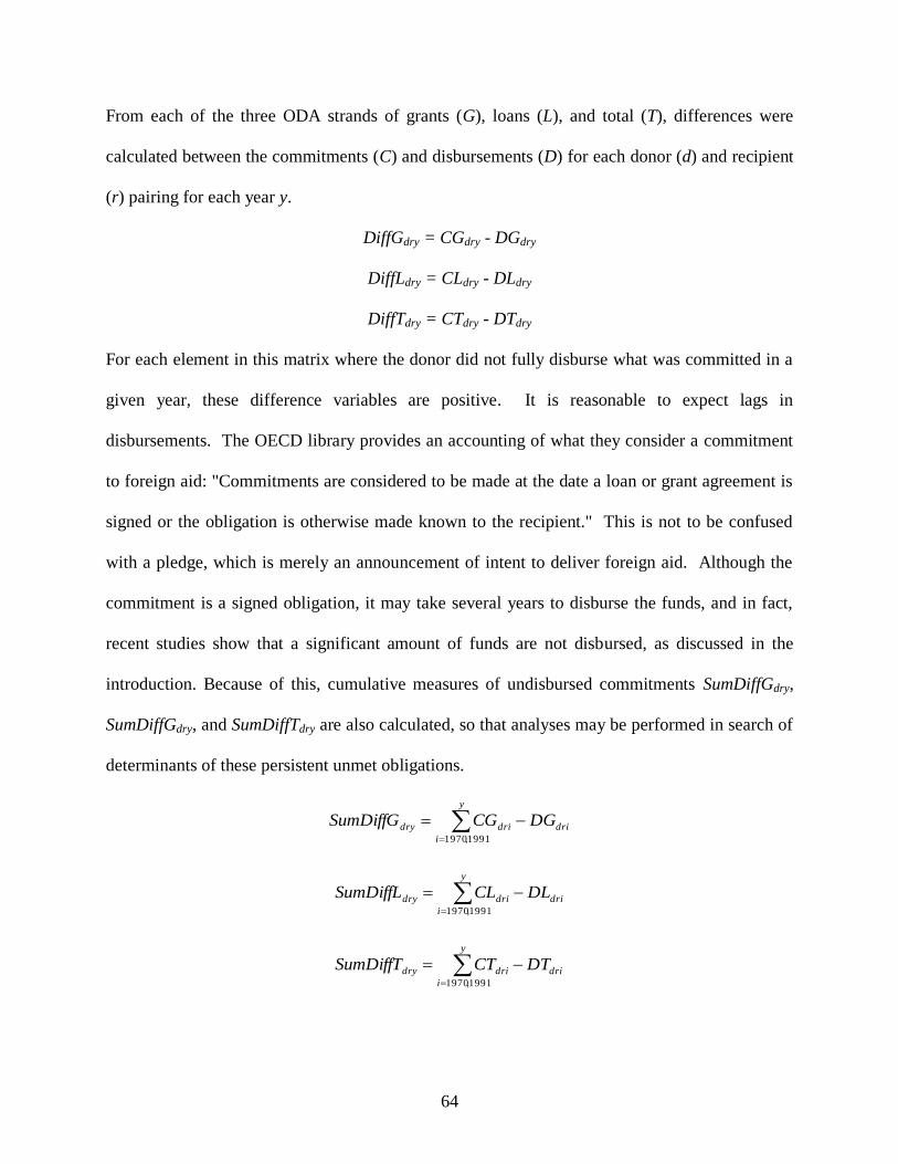
64
From each of the three ODA strands of grants (G), loans (L), and total (T), differences were
calculated between the commitments (C) and disbursements (D) for each donor (d) and recipient
(r) pairing for each year y.
DiffGdry = CGdry - DGdry
DiffLdry = CLdry - DLdry
DiffTdry = CTdry - DTdry
For each element in this matrix where the donor did not fully disburse what was committed in a
given year, these difference variables are positive. It is reasonable to expect lags in
disbursements. The OECD library provides an accounting of what they consider a commitment
to foreign aid: "Commitments are considered to be made at the date a loan or grant agreement is
signed or the obligation is otherwise made known to the recipient." This is not to be confused
with a pledge, which is merely an announcement of intent to deliver foreign aid. Although the
commitment is a signed obligation, it may take several years to disburse the funds, and in fact,
recent studies show that a significant amount of funds are not disbursed, as discussed in the
introduction. Because of this, cumulative measures of undisbursed commitments SumDiffGdry,
SumDiffGdry, and SumDiffTdry are also calculated, so that analyses may be performed in search of
determinants of these persistent unmet obligations.
y
i
dridridry DGCGSumDiffG1991,1970
y
i
dridridry DLCLSumDiffL1991,1970
y
i
dridridry DTCTSumDiffT1991,1970

65
Cumulative differences will not be generally comparable or even meaningful on a standalone
basis, given irregularities in the supply of data that force some nations to "begin" after others.
Although some data is available for the full 45 year span from 1966 through 2010, other data is
either limited or missing completely for certain nations. The same calculations were also
performed for the sub-period of 1991-2010 for comparison.
General information on ODA components by donor is available in Table 1. Nations are sorted
into two groups: original OECD nations, and then more recent entrants and non-OECD donor
nations.
Table 1: Summary Statistics of Foreign Aid, 1966 - 2010 (millions of 2010 USD)
DAC
Nation
Grant
Comm.
Grant
Disb.
Loan
Comm.
Loan
Disb.
Total
Comm.
Total
Disb.
TC/
TD
Austria $14,334 $13,196 $8,685 $5,974 $23,018 $15,613 1.47 Belgium $28,470 $30,775 $3,739 $3,763 $32,184 $33,321 0.97 Canada $65,662 $60,625 $16,596 $12,200 $82,261 $67,987 1.21 Denmark $29,938 $32,285 $5,927 $5,452 $35,865 $34,793 1.03 France $153,110 $161,125 $92,812 $73,346 $246,648 $197,190 1.25 Germany $154,843 $147,047 $104,067 $87,940 $258,964 $184,423 1.4 Greece $2,322 $2,322 $25 $25 $2,347 $2,347 1 Ireland $5,513 $5,703 $0 $0 $5,513 $5,703 0.97 Italy $46,343 $40,770 $38,105 $29,174 $79,457 $57,577 1.38 Luxembourg $2,652 $2,937 $0 $0 $2,652 $2,937 0.9 Netherlands $77,813 $77,426 $14,128 $12,255 $91,941 $81,811 1.12 Norway $42,452 $44,734 $825 $1,042 $43,278 $45,674 0.95 Portugal $3,839 $4,595 $1,807 $3,239 $5,647 $7,056 0.8 Spain $20,328 $23,598 $11,437 $14,846 $31,765 $33,158 0.96 Sweden $45,203 $45,059 $1,537 $1,437 $46,740 $45,855 1.02 Switzerland $24,569 $23,871 $1,473 $1,509 $26,061 $24,735 1.05 U.K. $108,354 $104,886 $26,874 $26,483 $137,001 $115,940 1.18 U.S. $404,778 $347,851 $106,677 $108,595 $523,307 $400,018 1.31 Australia $67,266 $65,557 $569 $465 $67,865 $65,942 1.03 Finland $11,438 $9,712 $1,078 $847 $12,517 $10,099 1.24 Japan $144,762 $140,748 $317,396 $242,882 $462,161 $270,176 1.71 Korea $3,120 $2,684 $7,081 $2,606 $10,201 $5,021 2.03 N. Zealand $5,082 $5,054 $45 $52 $5,126 $5,092 1.01 TOTAL $1,462,191 $1,392,560 $760,883 $634,132 $2,232,519 $1,712,468 1.3
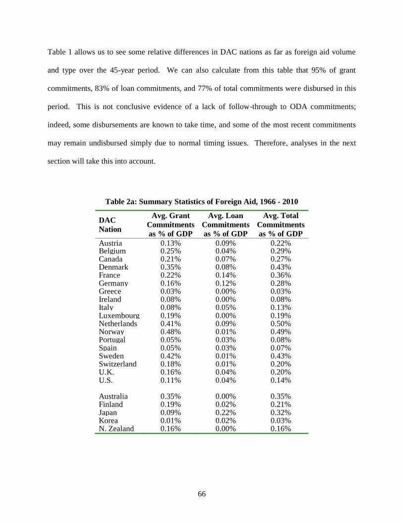
66
Table 1 allows us to see some relative differences in DAC nations as far as foreign aid volume
and type over the 45-year period. We can also calculate from this table that 95% of grant
commitments, 83% of loan commitments, and 77% of total commitments were disbursed in this
period. This is not conclusive evidence of a lack of follow-through to ODA commitments;
indeed, some disbursements are known to take time, and some of the most recent commitments
may remain undisbursed simply due to normal timing issues. Therefore, analyses in the next
section will take this into account.
Table 2a: Summary Statistics of Foreign Aid, 1966 - 2010
DAC
Nation
Avg. Grant
Commitments
as % of GDP
Avg. Loan
Commitments
as % of GDP
Avg. Total
Commitments
as % of GDP
Austria 0.13% 0.09% 0.22% Belgium 0.25% 0.04% 0.29% Canada 0.21% 0.07% 0.27% Denmark 0.35% 0.08% 0.43% France 0.22% 0.14% 0.36% Germany 0.16% 0.12% 0.28% Greece 0.03% 0.00% 0.03% Ireland 0.08% 0.00% 0.08% Italy 0.08% 0.05% 0.13% Luxembourg 0.19% 0.00% 0.19% Netherlands 0.41% 0.09% 0.50% Norway 0.48% 0.01% 0.49% Portugal 0.05% 0.03% 0.08% Spain 0.05% 0.03% 0.07% Sweden 0.42% 0.01% 0.43% Switzerland 0.18% 0.01% 0.20% U.K. 0.16% 0.04% 0.20% U.S. 0.11% 0.04% 0.14% Australia 0.35% 0.00% 0.35% Finland 0.19% 0.02% 0.21% Japan 0.09% 0.22% 0.32% Korea 0.01% 0.02% 0.03% N. Zealand 0.16% 0.00% 0.16%
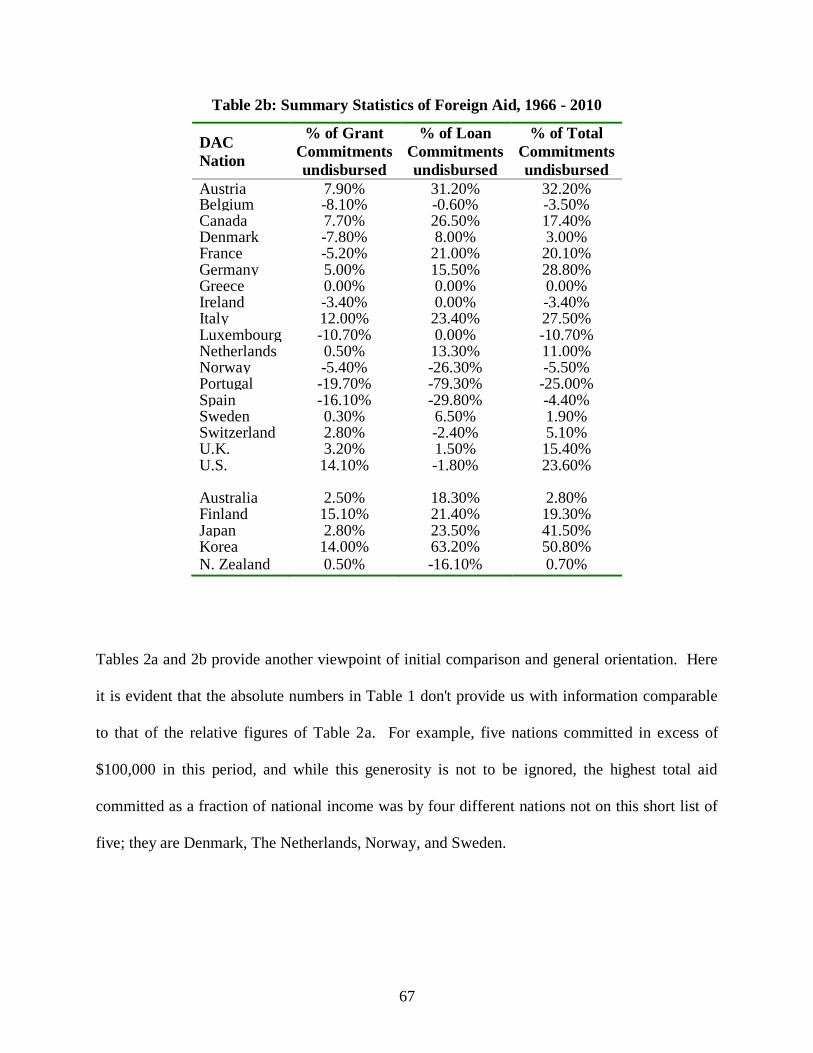
67
Table 2b: Summary Statistics of Foreign Aid, 1966 - 2010
DAC
Nation
% of Grant
Commitments
undisbursed
% of Loan
Commitments
undisbursed
% of Total
Commitments
undisbursed
Austria 7.90% 31.20% 32.20% Belgium -8.10% -0.60% -3.50% Canada 7.70% 26.50% 17.40% Denmark -7.80% 8.00% 3.00% France -5.20% 21.00% 20.10% Germany 5.00% 15.50% 28.80% Greece 0.00% 0.00% 0.00% Ireland -3.40% 0.00% -3.40% Italy 12.00% 23.40% 27.50% Luxembourg -10.70% 0.00% -10.70% Netherlands 0.50% 13.30% 11.00% Norway -5.40% -26.30% -5.50% Portugal -19.70% -79.30% -25.00% Spain -16.10% -29.80% -4.40% Sweden 0.30% 6.50% 1.90% Switzerland 2.80% -2.40% 5.10% U.K. 3.20% 1.50% 15.40% U.S. 14.10% -1.80% 23.60% Australia 2.50% 18.30% 2.80% Finland 15.10% 21.40% 19.30% Japan 2.80% 23.50% 41.50% Korea 14.00% 63.20% 50.80% N. Zealand 0.50% -16.10% 0.70%
Tables 2a and 2b provide another viewpoint of initial comparison and general orientation. Here
it is evident that the absolute numbers in Table 1 don't provide us with information comparable
to that of the relative figures of Table 2a. For example, five nations committed in excess of
$100,000 in this period, and while this generosity is not to be ignored, the highest total aid
committed as a fraction of national income was by four different nations not on this short list of
five; they are Denmark, The Netherlands, Norway, and Sweden.

68
Table 2b informs us of commitments that were not disbursed, and of those countries disbursing
aid in excess of commitments. We can see that there is a much greater volatility of loan
disbursements as a percentage of commitments relative to that of grants.
Table 3: Summary Statistics of Foreign Aid, 1966 - 2010
DAC Nation Employment
Average
Average
(geo)
growth
rate of
GDP
Number
of years of
GDP
decline
Avg.
Budget
Surplus,
% of GDP
# years of
Budget
Surplus
Austria 88.20% 2.50% 4 -2.10% 4 Belgium 84.90% 2.20% 4 -5.60% 2 Canada 82.80% 2.90% 3 -2.80% 12 Denmark 77.50% 1.90% 8 -0.50% 17 France 87.70% 2.30% 4 -3.20% 7 Germany 82.30% 2.00% 5 -2.80% 22 Greece 95.00% 2.40% 9 -5.40% 1 Ireland 88.10% 4.10% 4 -4.40% 10 Italy 92.60% 2.00% 5 -6.70% 0 Luxembourg 90.00% 3.80% 3 1.80% 35 Netherlands 70.50% 2.50% 3 -2.80% 6 Norway 73.30% 3.10% 2 6.00% 38 Portugal 91.00% 2.90% 7 -5.20% 6 Spain 92.50% 2.90% 4 -2.70% 5 Sweden 76.60% 2.10% 7 5.80% 20 Switzerland 70.50% 1.60% 7 -1.10% 23 United
Kingdom
76.30% 2.20% 7 -3.10% 5 United States 83.00% 2.90% 7 -3.30% 3 Australia 80.20% 3.20% 2 -1.70% 10 Finland 89.90% 2.60% 5 2.30% 31 Japan 2.60% 6 -3.00% 8 Korea 7.30% 2 2.10% 37 New Zealand 82.40% 2.30% 6 0.50% 29
In the next section, a cyclical derivative of GDP will be used to measure correlations with aid
flows, to determine cyclicality of aid. Employment is also used as a correlate with aid flows, for
a second business cycle proxy. Government budget surpluses as a percent of GDP will be used
with disbursement gap regressions as a control variable. Table 3 presents some basic
information about these variables for the same period of 1966 - 2010, (although GDP figures are
69
only from 1970 -2010). As noted earlier, unemployment is measured using national definitions,
so international comparisons are not meaningful. However, it is the annual percentage point
change that will be used for analysis, so this comparison is unnecessary.
2.3 Methods of Analysis and Results
This section explains and compares the methods used in estimating movements in the business
cycle, calculation of cumulative aid commitments, and tests of pro-cyclicality. Results of these
tests are presented, and the section ends with three extensions used as robustness checks on the
baseline analyses.
2.3.1 The Business Cycle
Business cycle fluctuations are measured with several proxies. One standard method of
calculation is a simple deviation from detrended GDP per capita, using a detrending technique
such as the Hodrick & Prescott (1997) filter, which is built on the assumption that a time-series
variable yt is composed of a growth (trend) component gt and a cyclical component ct such that yt
= gt + ct for t = 1,...,T. These components are calculated with minimization of the expression:
T
t
T
t
ttttt ggggc1 1
2
211
2
A smooth trend would indicate a near-constant growth figure; therefore, the difference between
growth and lagged growth for two consecutive periods should be very small. The HP filter
accounts for this by squaring this difference, and applying a multiplier λ on the sum of these
squares. A higher choice of λ then "penalizes" changes in the growth component over time.
There appears to be little consensus about the choice of this parameter for annual data; suggested
estimates range from a low of 6.5 (Ravn & Uhlig, 2002) or 10 (Backus & Kehoe, 1992) to 100
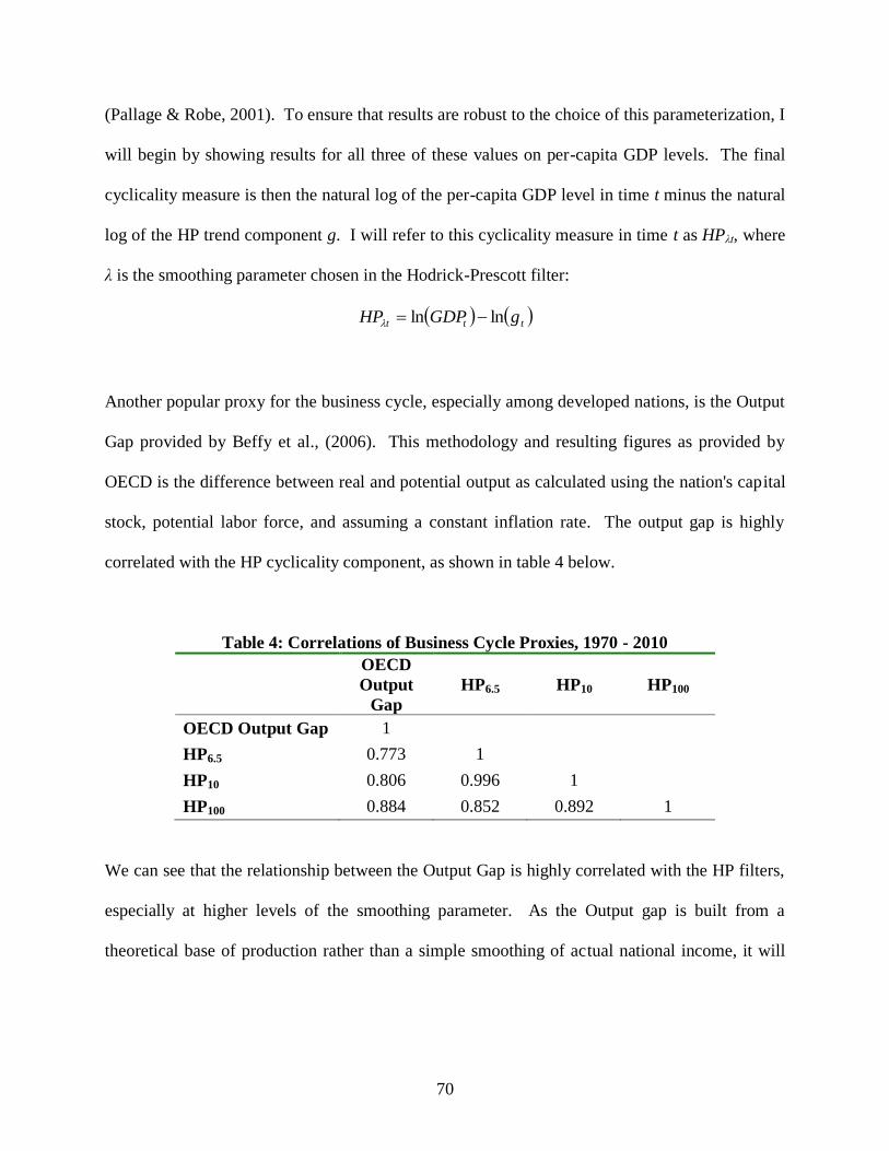
70
(Pallage & Robe, 2001). To ensure that results are robust to the choice of this parameterization, I
will begin by showing results for all three of these values on per-capita GDP levels. The final
cyclicality measure is then the natural log of the per-capita GDP level in time t minus the natural
log of the HP trend component g. I will refer to this cyclicality measure in time t as HPλt, where
λ is the smoothing parameter chosen in the Hodrick-Prescott filter:
ttt gGDPHP lnln
Another popular proxy for the business cycle, especially among developed nations, is the Output
Gap provided by Beffy et al., (2006). This methodology and resulting figures as provided by
OECD is the difference between real and potential output as calculated using the nation's capital
stock, potential labor force, and assuming a constant inflation rate. The output gap is highly
correlated with the HP cyclicality component, as shown in table 4 below.
Table 4: Correlations of Business Cycle Proxies, 1970 - 2010
OECD
Output
Gap
HP6.5 HP10 HP100
OECD Output Gap 1
HP6.5 0.773 1
HP10 0.806 0.996 1
HP100 0.884 0.852 0.892 1
We can see that the relationship between the Output Gap is highly correlated with the HP filters,
especially at higher levels of the smoothing parameter. As the Output gap is built from a
theoretical base of production rather than a simple smoothing of actual national income, it will

71
serve as more of a standard in subsequent analyses in measurement of business cycles and
shocks.27
2.3.2 Cyclicality of Aid
It has been generally found that aid tends to be pro-cyclical with donor income. While not the
focus of this paper, I begin by testing the cyclicality of commitments to confirm this finding in
the current dataset. Beginning with per-capital donor GDP in constant USD, each series is
detrended with the HP filter, creating HP6.5, HP10, and HP100 as shown in the previous section.
The OECD output gap is also used as a 4th sample of GDP cyclicality.
Recipient income, for purposes of subsequent analyses, is also detrended using the HP filter. A
low parameter value of λ=1, following Dabla-Norris et al. (2010) to allow for shorter business
cycles. The proxy for recipient cyclicality of income is then HP1. The majority of bilateral aid
flows are "missing values," of which nearly all are zeroes. It is not uncommon to then regard
these data points as zero aid flows, rather than to ignore them as missing values (Arndt et al.
2010; Dabla-Norris et al., 2010). This assumption is also used presently. Further, the OLS
regression coefficients can be considered elasticities if aid flows are transformed using a semi-
log form:
drydrydry GGsignG 1ln
drydrydry LLsignL 1ln
drydrydry TTsignT 1ln
27
This is true for donor nations, where OECD output gap data is available. Recipient nations
must be analyzed with HP filtered GDP levels.
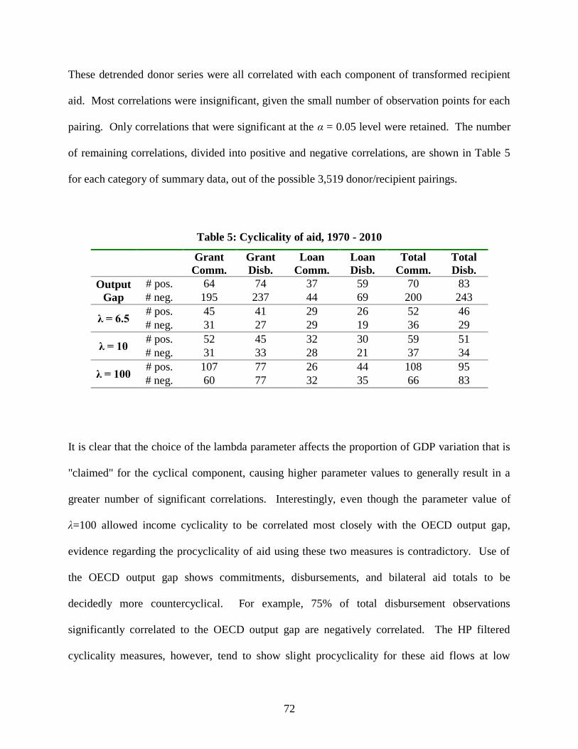
72
These detrended donor series were all correlated with each component of transformed recipient
aid. Most correlations were insignificant, given the small number of observation points for each
pairing. Only correlations that were significant at the α = 0.05 level were retained. The number
of remaining correlations, divided into positive and negative correlations, are shown in Table 5
for each category of summary data, out of the possible 3,519 donor/recipient pairings.
Table 5: Cyclicality of aid, 1970 - 2010
Grant
Comm.
Grant
Disb.
Loan
Comm.
Loan
Disb.
Total
Comm.
Total
Disb.
Output
Gap
# pos. 64 74 37 59 70 83
# neg. 195 237 44 69 200 243
λ = 6.5 # pos. 45 41 29 26 52 46
# neg. 31 27 29 19 36 29
λ = 10 # pos. 52 45 32 30 59 51
# neg. 31 33 28 21 37 34
λ = 100 # pos. 107 77 26 44 108 95
# neg. 60 77 32 35 66 83
It is clear that the choice of the lambda parameter affects the proportion of GDP variation that is
"claimed" for the cyclical component, causing higher parameter values to generally result in a
greater number of significant correlations. Interestingly, even though the parameter value of
λ=100 allowed income cyclicality to be correlated most closely with the OECD output gap,
evidence regarding the procyclicality of aid using these two measures is contradictory. Use of
the OECD output gap shows commitments, disbursements, and bilateral aid totals to be
decidedly more countercyclical. For example, 75% of total disbursement observations
significantly correlated to the OECD output gap are negatively correlated. The HP filtered
cyclicality measures, however, tend to show slight procyclicality for these aid flows at low
73
parameter values, and this preponderance grows as the lambda value increases. The exception to
this is the ambiguous procyclicality of HP filter correlations that relate to loan commitments.
The HP cyclicality measure is a popularly used proxy for the business cycle, and the OECD
output gap is quickly becoming more of an accepted standard, especially for donor nations.
However, it may be interesting to look at a third relative measure, such as the simple annual
change in employment. This variable was also calculated for each donor nation, for the years
1970-2008. The results of bilateral aid flow correlations with this variable are shown in Table 6.
Again, some procyclicality is demonstrated, as a positive change in employment in a donor
nation is more often correlated with aid. Interestingly, grants and total bilateral aid flows are
found to be somewhat procyclical here, in accordance with analyses in Table 5 using the HP
measure. Loan amounts appear countercyclical, more in line with the OECD output gap.
Table 6: Cyclicality of Aid, Correlations with Change in Employment, 1970 - 2008
Grant
Comm.
Grant
Disb.
Loan
Comm.
Loan
Disb.
Total
Comm.
Total
Disb.
# pos. 118 161 19 24 125 159
# neg. 118 129 58 69 114 117
We may opt to explore the data just a bit deeper at this point to examine whether, as purported in
past empirical works, the procyclicality of aid is particularly strong with respect to lower income
countries. The 153 recipient nations can easily be subdivided per the OECD classifications of
Least Developed Countries (LCDs), Low Income Countries (LICs), Low Middle Income
Countries (LMICs), and Upper Middle Income Countries (UMICs). With these four categories
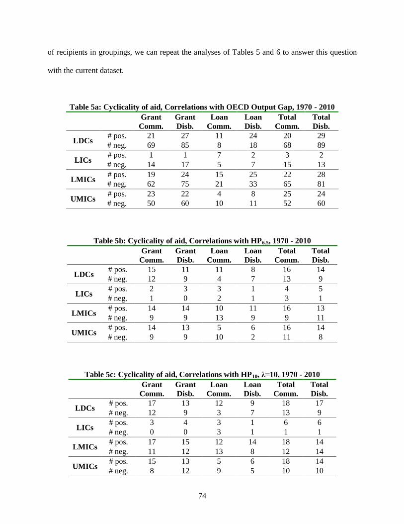
74
of recipients in groupings, we can repeat the analyses of Tables 5 and 6 to answer this question
with the current dataset.
Table 5a: Cyclicality of aid, Correlations with OECD Output Gap, 1970 - 2010
Grant
Comm.
Grant
Disb.
Loan
Comm.
Loan
Disb.
Total
Comm.
Total
Disb.
LDCs # pos. 21 27 11 24 20 29
# neg. 69 85 8 18 68 89
LICs # pos. 1 1 7 2 3 2
# neg. 14 17 5 7 15 13
LMICs # pos. 19 24 15 25 22 28
# neg. 62 75 21 33 65 81
UMICs # pos. 23 22 4 8 25 24
# neg. 50 60 10 11 52 60
Table 5b: Cyclicality of aid, Correlations with HP6.5, 1970 - 2010
Grant
Comm.
Grant
Disb.
Loan
Comm.
Loan
Disb.
Total
Comm.
Total
Disb.
LDCs # pos. 15 11 11 8 16 14
# neg. 12 9 4 7 13 9
LICs # pos. 2 3 3 1 4 5
# neg. 1 0 2 1 3 1
LMICs # pos. 14 14 10 11 16 13
# neg. 9 9 13 9 9 11
UMICs # pos. 14 13 5 6 16 14
# neg. 9 9 10 2 11 8
Table 5c: Cyclicality of aid, Correlations with HP10, λ=10, 1970 - 2010
Grant
Comm.
Grant
Disb.
Loan
Comm.
Loan
Disb.
Total
Comm.
Total
Disb.
LDCs # pos. 17 13 12 9 18 17
# neg. 12 9 3 7 13 9
LICs # pos. 3 4 3 1 6 6
# neg. 0 0 3 1 1 1
LMICs # pos. 17 15 12 14 18 14
# neg. 11 12 13 8 12 14
UMICs # pos. 15 13 5 6 18 14
# neg. 8 12 9 5 10 10

75
Table 5d: Cyclicality of aid, Correlations with HP100, 1970 - 2010
Grant
Comm.
Grant
Disb.
Loan
Comm.
Loan
Disb.
Total
Comm.
Total
Disb.
LDCs # pos. 31 21 9 17 32 27
# neg. 18 21 7 11 17 22
LICs # pos. 7 4 2 1 9 6
# neg. 3 4 6 4 5 4
LMICs # pos. 36 25 10 18 35 32
# neg. 24 29 8 11 25 34
UMICs # pos. 33 27 5 8 32 30
# neg. 15 23 11 9 19 23
Table 6a: Cyclicality of Aid, Correlations with Change in Employment, 1970 - 2008
Grant
Comm.
Grant
Disb.
Loan
Comm.
Loan
Disb.
Total
Comm.
Total
Disb.
LDCs # pos. 36 62 6 8 42 62
# neg. 32 38 15 16 39 35
LICs # pos. 16 20 2 5 18 19
# neg. 17 17 5 9 17 13
LMICs # pos. 37 46 7 8 38 47
# neg. 41 47 26 30 38 36
UMICs # pos. 29 33 4 3 27 31
# neg. 28 27 12 14 30 33
A similar dichotomy is shown in Tables 5a-5d and 6a, where the OECD output gap tends to
show the opposite relationship with most aid flows than does the cyclicality measure derived
from the HP filter. Focusing on the Least Developed Countries (LDCs), the output gap has more
significantly negative correlations with most bilateral aid flow types, indicating a tendency to be
countercyclical. These same transformed aid flows to the poorest countries are more correlated
with HP income procyclicality, again with generally stronger ratios as the parameter is increased.
Table 5 shows that employment changes are also positively correlated with bilateral aid flows to
the poorest countries, providing more evidence for procyclicality.
76
2.3.3 Undisbursed Commitments
The main focus of this paper is to examine the difference between commitments and
disbursements, and to explore whether this difference is related to the business cycle of the donor
country. We can start by noting that Table 2 gives us a clear picture of the variance between
nations with regard to undisbursed commitments. Some nations, such as Korea, allow up to half
of their committed foreign aid to remain undisbursed during this time period, while other nations
such as Luxembourg and Portugal actually give substantially more aid than they promise. It is
quite likely that these differences rest on multiple variables, only a few of which will be
explored. But any overall measure of undisbursed commitments would average these fixed
effects, losing much information about these overall differences between nations.
The differences of DiffGdry, DiffLdry, and DiffTdry have been calculated as shown, and have also
undergone the semi-log transformation used for previous aid figures. The results are now
correlated with the OECD output gap as the business cycle proxy, as were the six individual aid
flows themselves. The correlations for each donor nation are shown in Table 7.
With Table 7, we can see a marked difference between the cyclicality of bilateral aid flows and
the payment of committed bilateral aid flows. Recall from section 3.2 that the aid flows were
consistently shown to be countercyclical in correlations with the OECD output gap. Here, the
output gap is generally procyclically correlated with disbursement gaps. The majority of
correlations (69%) in Table 7 are positive.

77
Table 7: Disbursement Gap Correlations with the OECD Output Gap, 1970 - 2010
DAC Nation Grant
Gap
Loan
Gap
Total
Gap
Grant
Gap
(LDCs
only)
Loan
Gap
(LDCs
only)
Total
Gap
(LDCs
only)
Austria -0.216 -0.031 0.128 -0.111 0.209 0.054
Belgium 0.237 -0.020 0.191 0.280* 0.091 0.242
Canada 0.137 -0.075 0.178 0.156 0.237 0.364**
Denmark 0.140 0.152 0.053 0.128 0.040 0.270*
France 0.186 0.005 0.104 0.135 -0.323**
-0.089
Germany -0.400* -0.146 -0.279 -0.168 0.045 -0.107
Greece 0.055
Ireland
Italy -0.240 0.029 0.110 -0.178 -0.099 -0.173
Luxembourg -0.200 -0.200 0.235 0.235
Netherlands 0.266* 0.173 0.319
** 0.342
** 0.022 0.375
**
Norway 0.256 -0.407**
0.226 0.091 0.032 0.098
Portugal 0.001 -0.282 -0.117 -0.012 -0.382**
-0.126
Spain -0.053 0.196 0.391**
-0.053 -0.113 0.237
Sweden 0.006 0.046 -0.088 -0.022 0.064 -0.091
Switzerland 0.448**
0.112 0.476***
0.229 0.210
United Kingdom 0.386**
0.090 0.506***
0.342***
0.188 0.438***
United States 0.223 0.249 0.063 0.111 0.082 0.144
Australia 0.147 0.266* 0.163 0.307
* 0.307
*
Finland 0.295* 0.238 0.310
* 0.041 0.201 0.123
Japan -0.102 0.178 -0.021 0.013 -0.066 -0.069
Korea
New Zealand -0.112 -0.112 0.040 0.040
Significance of these correlations at the 10%, 5%, and 1% levels
are denoted by *, **, and *** respectively.
In the right three columns, the same calculations are shown for just the 49 LDCs, in case a
similar bias was found as in Tables 4a and 5a. Because of the relatively small number of
disbursement gaps, few of the correlations are highly significant. It is not clear from browsing
this grid of numbers whether the disbursement gaps are necessarily more procyclical for LDCs,
but 70% these of correlations are positive, comparable to 69% for the entire sample. A simple
average of these correlations across numbers provides only about 0.080 for total aid, and 0.082
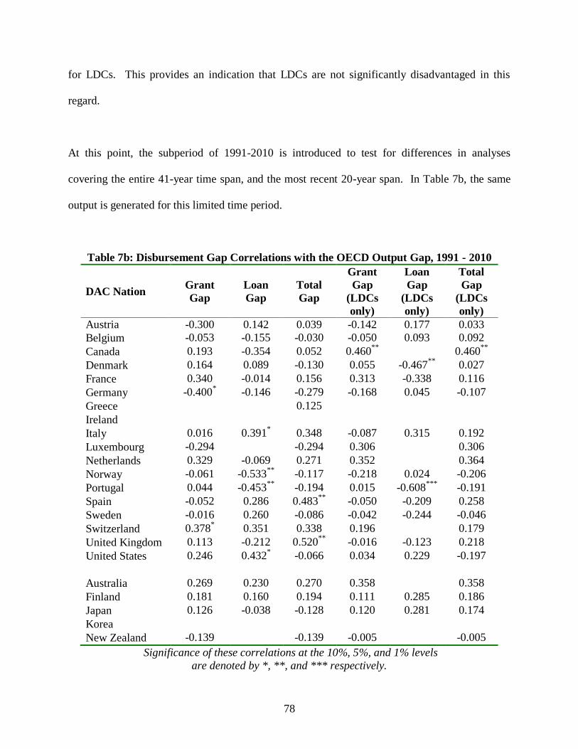
78
for LDCs. This provides an indication that LDCs are not significantly disadvantaged in this
regard.
At this point, the subperiod of 1991-2010 is introduced to test for differences in analyses
covering the entire 41-year time span, and the most recent 20-year span. In Table 7b, the same
output is generated for this limited time period.
Table 7b: Disbursement Gap Correlations with the OECD Output Gap, 1991 - 2010
DAC Nation Grant
Gap
Loan
Gap
Total
Gap
Grant
Gap
(LDCs
only)
Loan
Gap
(LDCs
only)
Total
Gap
(LDCs
only)
Austria -0.300 0.142 0.039 -0.142 0.177 0.033
Belgium -0.053 -0.155 -0.030 -0.050 0.093 0.092
Canada 0.193 -0.354 0.052 0.460**
0.460**
Denmark 0.164 0.089 -0.130 0.055 -0.467**
0.027
France 0.340 -0.014 0.156 0.313 -0.338 0.116
Germany -0.400* -0.146 -0.279 -0.168 0.045 -0.107
Greece 0.125
Ireland
Italy 0.016 0.391* 0.348 -0.087 0.315 0.192
Luxembourg -0.294 -0.294 0.306 0.306
Netherlands 0.329 -0.069 0.271 0.352 0.364
Norway -0.061 -0.533**
-0.117 -0.218 0.024 -0.206
Portugal 0.044 -0.453**
-0.194 0.015 -0.608***
-0.191
Spain -0.052 0.286 0.483**
-0.050 -0.209 0.258
Sweden -0.016 0.260 -0.086 -0.042 -0.244 -0.046
Switzerland 0.378* 0.351 0.338 0.196 0.179
United Kingdom 0.113 -0.212 0.520**
-0.016 -0.123 0.218
United States 0.246 0.432* -0.066 0.034 0.229 -0.197
Australia 0.269 0.230 0.270 0.358 0.358
Finland 0.181 0.160 0.194 0.111 0.285 0.186
Japan 0.126 -0.038 -0.128 0.120 0.281 0.174
Korea
New Zealand -0.139 -0.139 -0.005 -0.005
Significance of these correlations at the 10%, 5%, and 1% levels
are denoted by *, **, and *** respectively.

79
The average correlation in this subsample drops with the earliest years removed, to 0.053 for the
entire sample, and 0.059 for the LDC countries. A reduction in procyclicality of the
disbursement gap is also indicated by the raw count of positive correlations. Where the 41-year
sample showed 69% of correlations to be positive, this subsample shows just 58% of correlations
to be positive.
2.3.4 Cumulative Undisbursed Commitments
A simple comparison of commitments and disbursements from year to year provided some
evidence that the business cycle is related to the timing of fund disbursements. Some evidence
was found for procyclicality for the disbursement gap in the previous section. However, what
may be more telling is the cumulative undisbursed funds committed from each donor to each
recipient. To facilitate this, a simple variable of cumulative normalized commitments, Ccum, is
calculated for each donor/recipient pairing for each year. Again, a semi-log transformation of
this cumulative undisbursed balance is used in analyses.
We may again run correlations in order to search for a simple preponderance of positive or
negative values, with few significant results. However, a multivariate regression of this
distribution gap over the 41-year period and 20-year subperiod would allow us to include control
variables that may provide a better idea as to some of the factors that influence this timing.
The cyclicality of donor income is the main variable of focus; however, is this relationship robust
through varying fiscal stances? Perhaps the donor nation's budget surplus as a percentage of
80
GDP is also related to the ease with which disbursements of aid flow to recipient nations. And
what of recipient GDP, or even relative GDP between the donor and the recipient? We have
seen that LDCs tend to receive the most procyclical funding; is this relationship true of the
disbursement gap as well? And finally, is it reasonable to expect that the donor nation may make
disbursement decisions in part based on the cyclicality of the recipient nation's income per
capita?
To answer these questions, the matrices of SumDiffGdry, SumDiffGdry, and SumDiffGdry are
calculated, each normalized again by division of GDP in the year y of analysis, and regressed
with the equations:
drddrddry CycSumDiffG
drddrddry CycSumDiffL
drddrddry CycSumDiffT
where Cycd is the vector over the 41-year period of the cyclical component of donor income per
capita, and the omega matrix is a series of control variables such as the donor's budget surplus as
a percentage of GDP, total donor GDP per capita, total recipient GDP per capita, the ratio of
donor/recipient per capita GDP, the size of the aid flow, and the cyclicality of recipient GDP per
capita.
The analysis begins with OLS regressions without the omega vector; only the lone regressor of
the donor's cyclical component of income was used. The dataset includes 23 donors, 153
recipients, and three aid flow types, which allows for just over 10,000 potential regressions to be
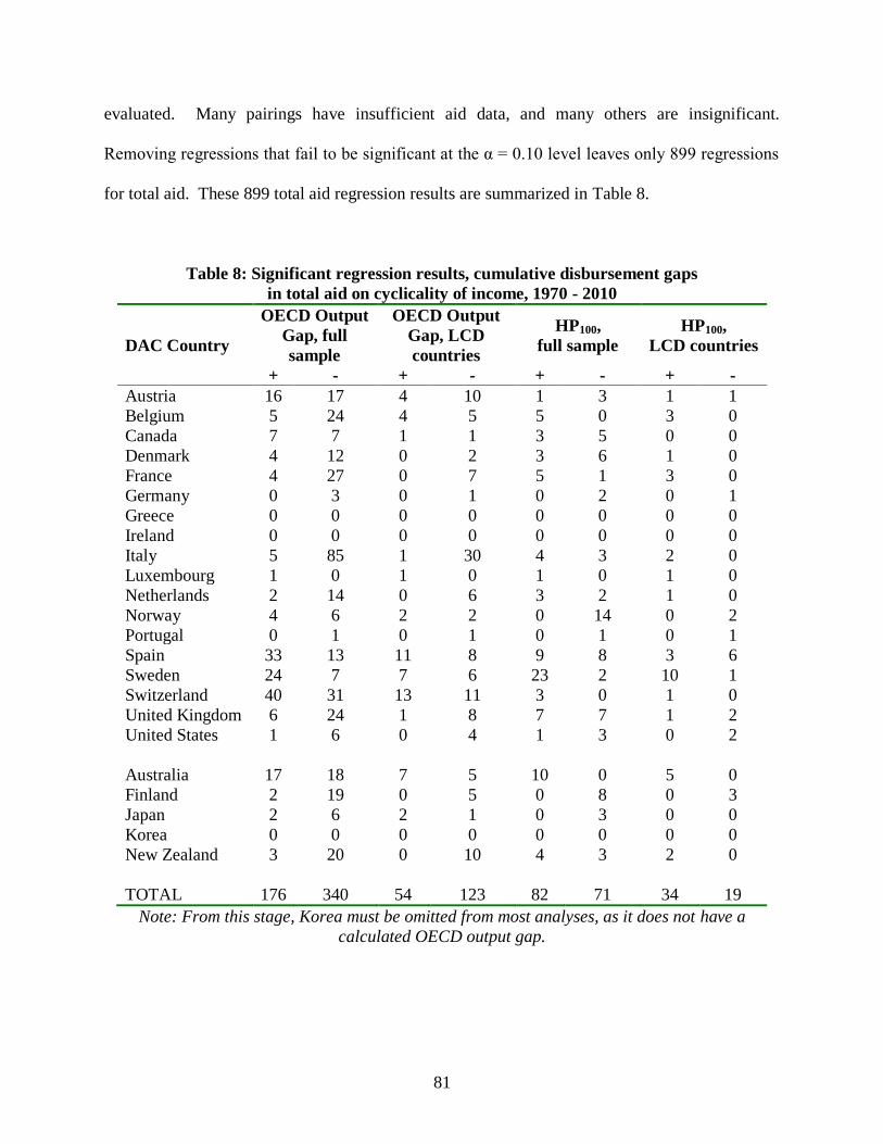
81
evaluated. Many pairings have insufficient aid data, and many others are insignificant.
Removing regressions that fail to be significant at the α = 0.10 level leaves only 899 regressions
for total aid. These 899 total aid regression results are summarized in Table 8.
Table 8: Significant regression results, cumulative disbursement gaps
in total aid on cyclicality of income, 1970 - 2010
DAC Country
OECD Output
Gap, full
sample
OECD Output
Gap, LCD
countries
HP100,
full sample
HP100,
LCD countries
+ - + - + - + -
Austria 16 17 4 10 1 3 1 1
Belgium 5 24 4 5 5 0 3 0
Canada 7 7 1 1 3 5 0 0
Denmark 4 12 0 2 3 6 1 0
France 4 27 0 7 5 1 3 0
Germany 0 3 0 1 0 2 0 1
Greece 0 0 0 0 0 0 0 0
Ireland 0 0 0 0 0 0 0 0
Italy 5 85 1 30 4 3 2 0
Luxembourg 1 0 1 0 1 0 1 0
Netherlands 2 14 0 6 3 2 1 0
Norway 4 6 2 2 0 14 0 2
Portugal 0 1 0 1 0 1 0 1
Spain 33 13 11 8 9 8 3 6
Sweden 24 7 7 6 23 2 10 1
Switzerland 40 31 13 11 3 0 1 0
United Kingdom 6 24 1 8 7 7 1 2
United States 1 6 0 4 1 3 0 2
Australia 17 18 7 5 10 0 5 0
Finland 2 19 0 5 0 8 0 3
Japan 2 6 2 1 0 3 0 0
Korea 0 0 0 0 0 0 0 0
New Zealand 3 20 0 10 4 3 2 0
TOTAL 176 340 54 123 82 71 34 19
Note: From this stage, Korea must be omitted from most analyses, as it does not have a
calculated OECD output gap.

82
Note that a majority of negative coefficients indicates that business cycle booms are related to an
decrease in the donor's disbursement gap. A summary across the DAC donor countries leaves
initial evidence of countercyclical disbursement gaps with the OECD output gap, and procyclical
disbursement gaps with the HP cyclicality measure, much as before. We do not see any
noticeable difference among the poorest countries.
These results are without any control variables that may also have significant relation to the
timing of disbursements. Also, we may interpret procyclicality here as either relating to a
reduced incidence of payment, or a higher incidence of commitment. A conditional lag will be
introduced later to address this question.
For a closer initial investigation, the omega vector is now added to the matrix of regression
results. Fixed effects variables are used for each donor/recipient pairing. Table 9 shows the
results of three specifications across all donors, recipients, and time periods.
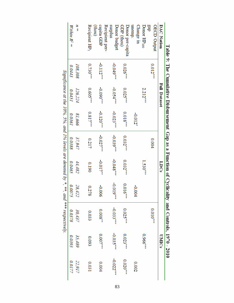
83
84
In Table 9, we can see several consistencies in relation to the disbursement gap. First, the
incidence of undisbursed commitments in a given year is clearly procyclical for the donor. Both
the OECD output gap and the cyclical component of donor income are positively related to the
disbursement gap. This relationship is very highly significant in most specifications, while
unemployment change is a weak indicator.
Across all specifications, the control variables are much the same. Greater donor income per
capita is related to larger disbursement gaps. However, it is quite possible that this relationship
may be due to slower movements in the governments of wealthier nations. The conditional lag,
investigated next, will provide some clues as to whether this may be the case. Donor budget
surplus is negatively related to the disbursement gap. Nations with budget surpluses appear
more likely to pay their commitments immediately. The reader may question whether this
relationship is really just a fiscal stance in relation to the business cycle of the donor country.
This is possible. The correlation between this budget surplus ratio and the OECD output gap is
0.40, and the correlation between budget surplus and the detrended cyclicality measure is 0.29.
But given that these correlations are not extremely high, and that foreign aid disbursements and
budgetary decisions are typically made by different factions of a government, this control
variable is retained.
Recipient GDP is significantly related to the disbursement gap in the full sample, with wealthier
recipient nations receiving more timely disbursements. There may be a nonlinearity in this
relationship, as the wealthiest recipient countries show positive coefficients on this control
variable, suggesting that the wealthiest nations in this group suffer from larger disbursement
85
gaps. Interestingly, the business cycle of the recipient nation appears positively related to the
disbursement gap in the full sample specifications. Donors are more likely to pay less on their
commitments when recipient income is above trend. Again, the disbursement gap is a
combination of both commitments and payments, the timing of which is hidden in this initial
analysis.
In Table 9b, we are able to see the same regressions for the more recent subset of 1991-2010.
Within this 20-year time frame, we can see that the disbursement gap remains procyclical for
both measures of cyclicality, although not so for LDCs. Employment changes remains a poor
predictor of the disbursement gap. Wealthier donor nations still tend to have larger disbursement
gaps, larger budget surpluses reduce the disbursement gap, and cumulative disbursement gaps
grow as recipient nations show above trend income, as was the case in the full 41-year dataset.
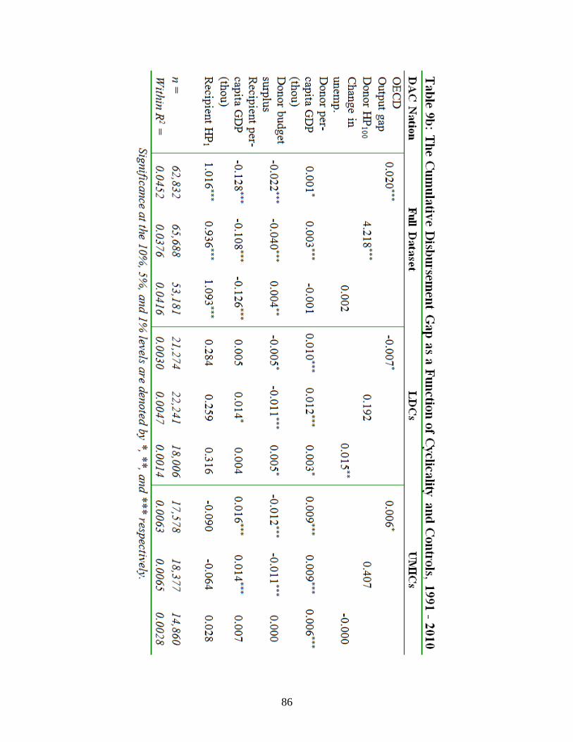
86
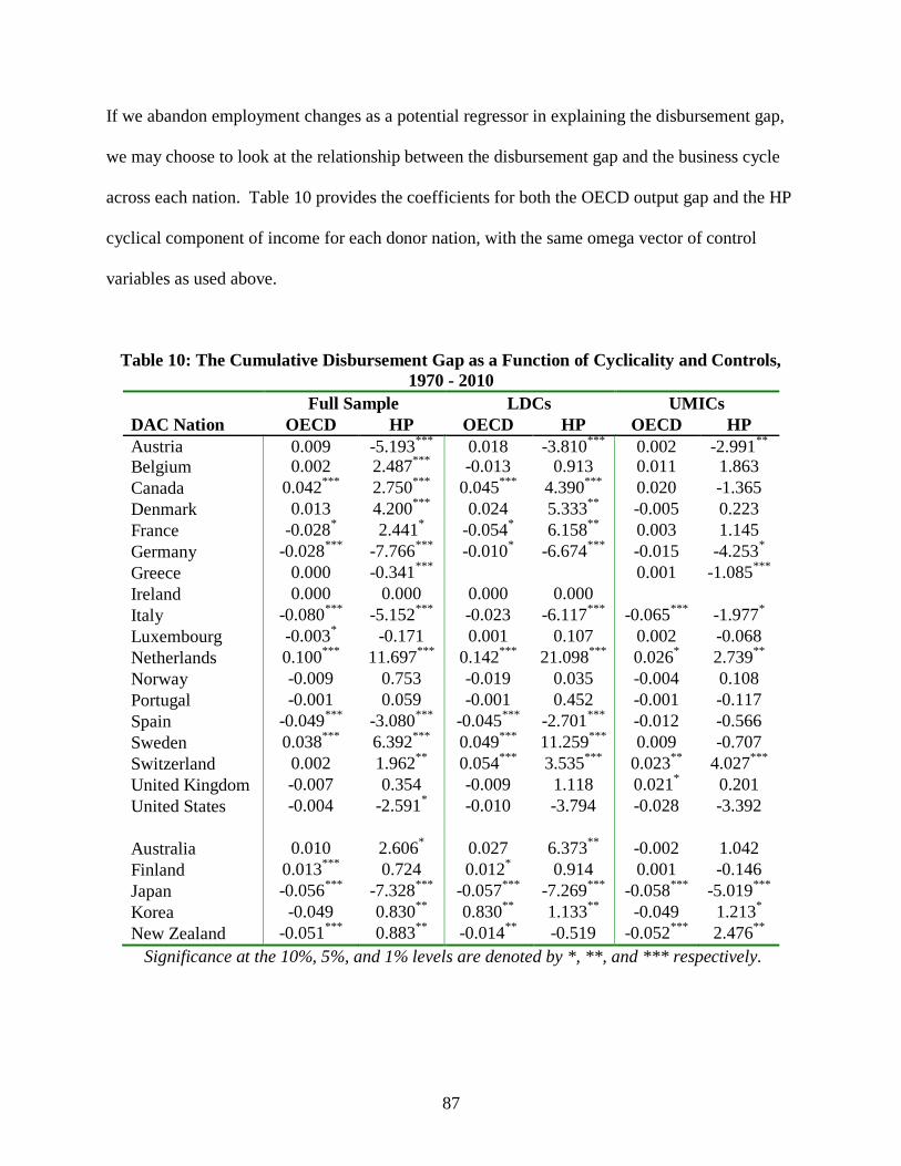
87
If we abandon employment changes as a potential regressor in explaining the disbursement gap,
we may choose to look at the relationship between the disbursement gap and the business cycle
across each nation. Table 10 provides the coefficients for both the OECD output gap and the HP
cyclical component of income for each donor nation, with the same omega vector of control
variables as used above.
Table 10: The Cumulative Disbursement Gap as a Function of Cyclicality and Controls,
1970 - 2010
Full Sample LDCs UMICs
DAC Nation OECD HP OECD HP OECD HP
Austria 0.009 -5.193***
0.018 -3.810***
0.002 -2.991**
Belgium 0.002 2.487***
-0.013 0.913 0.011 1.863
Canada 0.042***
2.750***
0.045***
4.390***
0.020 -1.365
Denmark 0.013 4.200***
0.024 5.333**
-0.005 0.223
France -0.028* 2.441
* -0.054
* 6.158
** 0.003 1.145
Germany -0.028***
-7.766***
-0.010* -6.674
*** -0.015 -4.253
*
Greece 0.000 -0.341***
0.001 -1.085***
Ireland 0.000 0.000 0.000 0.000
Italy -0.080***
-5.152***
-0.023 -6.117***
-0.065***
-1.977*
Luxembourg -0.003* -0.171 0.001 0.107 0.002 -0.068
Netherlands 0.100***
11.697***
0.142***
21.098***
0.026* 2.739
**
Norway -0.009 0.753 -0.019 0.035 -0.004 0.108
Portugal -0.001 0.059 -0.001 0.452 -0.001 -0.117
Spain -0.049***
-3.080***
-0.045***
-2.701***
-0.012 -0.566
Sweden 0.038***
6.392***
0.049***
11.259***
0.009 -0.707
Switzerland 0.002 1.962**
0.054***
3.535***
0.023**
4.027***
United Kingdom -0.007 0.354 -0.009 1.118 0.021* 0.201
United States -0.004 -2.591* -0.010 -3.794 -0.028 -3.392
Australia 0.010 2.606* 0.027 6.373
** -0.002 1.042
Finland 0.013***
0.724 0.012* 0.914 0.001 -0.146
Japan -0.056***
-7.328***
-0.057***
-7.269***
-0.058***
-5.019***
Korea -0.049 0.830**
0.830**
1.133**
-0.049 1.213*
New Zealand -0.051***
0.883**
-0.014**
-0.519 -0.052***
2.476**
Significance at the 10%, 5%, and 1% levels are denoted by *, **, and *** respectively.

88
Using the OECD output gap as a regressor for the full sample, 9 of the 23 DAC donor nations
show a coefficient significant at a minimum of the α = 0.05 level. Of these, 4 are positive,
providing no further evidence of procyclicality of the cumulative disbursement gap with this
measure. Using the HP filter, there are 13 significant regressors in this table, and 7 of these are
positive. Again, no procyclicality of the disbursement gap is evident here. This is similar to the
results in the LDC subset, where 4 of 7 significant regressors are positive for the output gap, and
7 of 12 for the HP filter. The general result from these baseline analyses is that there appears to
be no evidence suggesting that the disbursement gap from year to year across donor nations
tends to be procyclical or countercyclical with donor income, even though the cumulative
disbursement gap has been shown to be significantly procyclical overall.
In the most recent subsample, the results are similar. There are 9 significant coefficients (again,
at the α = 0.05 level) on the OECD output gap in the full subsample, and 7 of those are negative,
indicating a potential shift toward countercyclicality of the disbursement gap in recent decades.
Results for the HP filtered cyclicality measure are neutral, with 5 of 11 positive and significant
coefficients. A cursory glance at the results for low income countries over this time period
suggests that the disbursement gap is becoming more countercyclical for these nations as well.
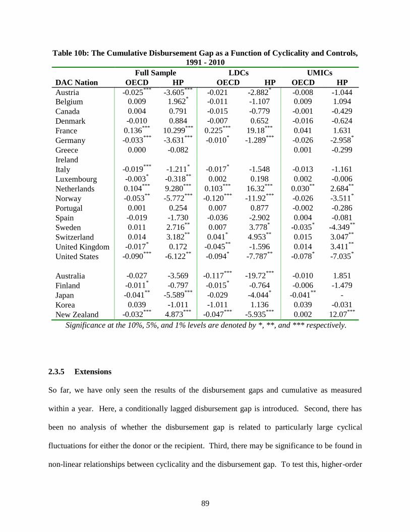
89
Table 10b: The Cumulative Disbursement Gap as a Function of Cyclicality and Controls,
1991 - 2010
Full Sample LDCs UMICs
DAC Nation OECD HP OECD HP OECD HP
Austria -0.025***
-3.605***
-0.021 -2.882* -0.008 -1.044
Belgium 0.009 1.962* -0.011 -1.107 0.009 1.094
Canada 0.004 0.791 -0.015 -0.779 -0.001 -0.429
Denmark -0.010 0.884 -0.007 0.652 -0.016 -0.624
France 0.136***
10.299***
0.225***
19.18***
0.041 1.631
Germany -0.033***
-3.631***
-0.010* -1.289
*** -0.026 -2.958
*
Greece 0.000 -0.082 0.001 -0.299
Ireland
Italy -0.019***
-1.211* -0.017
* -1.548 -0.013 -1.161
Luxembourg -0.003* -0.318
** 0.002 0.198 0.002 -0.006
Netherlands 0.104***
9.280***
0.103***
16.32***
0.030**
2.684**
Norway -0.053**
-5.772***
-0.120***
-11.92***
-0.026 -3.511*
Portugal 0.001 0.254 0.007 0.877 -0.002 -0.286
Spain -0.019 -1.730 -0.036 -2.902 0.004 -0.081
Sweden 0.011 2.716**
0.007 3.778* -0.035
* -4.349
**
Switzerland 0.014 3.182**
0.041* 4.953
** 0.015 3.047
**
United Kingdom -0.017* 0.172 -0.045
** -1.596 0.014 3.411
**
United States -0.090***
-6.122**
-0.094* -7.787
** -0.078
* -7.035
*
Australia -0.027 -3.569 -0.117***
-19.72***
-0.010 1.851
Finland -0.011* -0.797 -0.015
* -0.764 -0.006 -1.479
Japan -0.041**
-5.589***
-0.029 -4.044* -0.041
** -
4.121***
Korea 0.039 -1.011 -1.011 1.136 0.039 -0.031
New Zealand -0.032***
4.873***
-0.047***
-5.935***
0.002 12.07***
Significance at the 10%, 5%, and 1% levels are denoted by *, **, and *** respectively.
2.3.5 Extensions
So far, we have only seen the results of the disbursement gaps and cumulative as measured
within a year. Here, a conditionally lagged disbursement gap is introduced. Second, there has
been no analysis of whether the disbursement gap is related to particularly large cyclical
fluctuations for either the donor or the recipient. Third, there may be significance to be found in
non-linear relationships between cyclicality and the disbursement gap. To test this, higher-order
90
terms for the cyclical regressors may be explored. Fourth, the best known target for DAC
nations in bilateral foreign aid is a 0.7% of GNI target. As this is measured by disbursements
rather than commitments, this threshold may induce commitments to be more likely backed by
cash. In this section, these additional tests will be presented.
We start with the addition of cubed cyclical variables and the introduction of two "large negative
shock" dummy variables; one for donors, and another for recipients. For donor nations, this
variable is one if the OECD output gap of a donor nation is in the lowest 5% of the output gaps
in the total sample, and zero otherwise. For recipient nations, this variable is one if the semi-log
transformed HP filtered cyclicality measure is in the lowest 10% of values across all recipient
observations. The percentile level of 5% was chosen arbitrarily, in order to capture the worst
downturns of the donors. The 10% level was chosen with a simple supposition that unfavorable
shocks are perhaps twice as likely in recipient nations. In the dataset, there is evidence that the
poorest countries have a disproportionate share of large negative shocks. The LDCs in the
dataset are shown to have large negative shocks 11.8% of the time with this measure.

91
92
Adding these new variables to the original omega vector used previously allows for several
specifications, which are displayed in Table 11. Across the entire sample, procyclicality of the
cumulative disbursement gap continues to be predominant, using either measure of cyclicality.
The cubed cyclicality measures are not significant across the full sample, but especially large
movements from trend appear to be especially disadvantageous to the poorest recipient nations.
Large negative shocks to donor income tend to reduce the disbursement gap, as do large negative
shocks to recipient income. This is a welcome result, as we tend to think of foreign aid as being
particularly relevant to circumstances of recipient downturns. With these additional controls, it
is clear that lower income donor countries and donor nations with higher budget surpluses
continue to have smaller disbursement gaps. Also, evidence is consistent that wealthier
recipients collect more of their bilateral aid commitments. Most of these regularities are also
true for the subsample of LDCs. Finally, the cyclicality of recipient income appears to be less
related to the cumulative disbursement gap with these additional control variables.
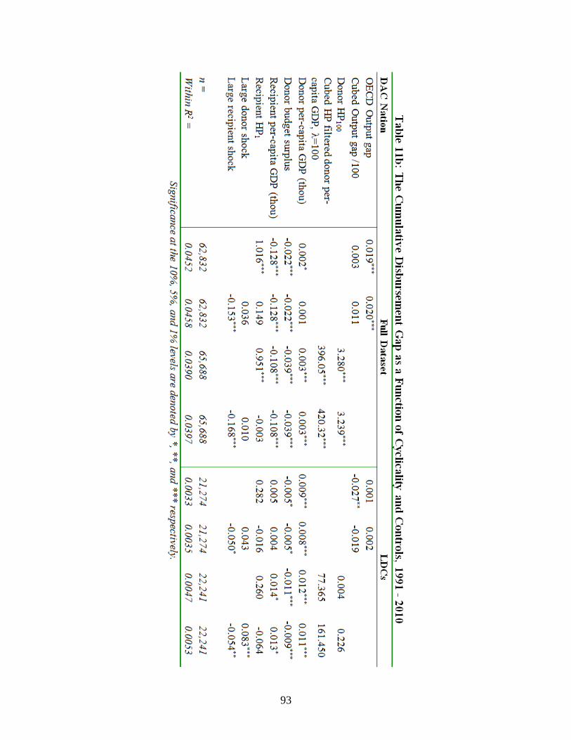
93
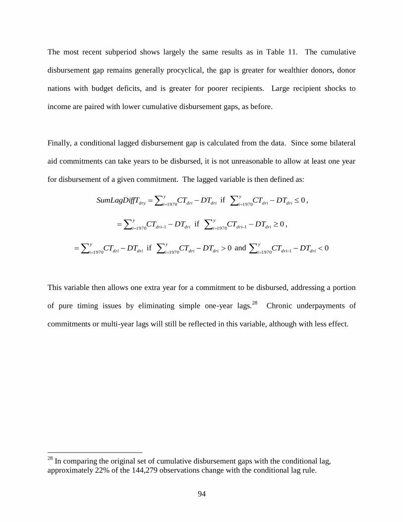
94
The most recent subperiod shows largely the same results as in Table 11. The cumulative
disbursement gap remains generally procyclical, the gap is greater for wealthier donors, donor
nations with budget deficits, and is greater for poorer recipients. Large recipient shocks to
income are paired with lower cumulative disbursement gaps, as before.
Finally, a conditional lagged disbursement gap is calculated from the data. Since some bilateral
aid commitments can take years to be disbursed, it is not unreasonable to allow at least one year
for disbursement of a given commitment. The lagged variable is then defined as:
y
i dridridry DTCTTSumLagDiff1970
if 01970
y
i dridri DTCT ,
y
i dridri DTCT1970 1
if 01970 1
y
i dridri DTCT ,
y
i dridri DTCT1970
if 01970
y
i dridri DTCT and 01970 1
y
i dridri DTCT
This variable then allows one extra year for a commitment to be disbursed, addressing a portion
of pure timing issues by eliminating simple one-year lags.28
Chronic underpayments of
commitments or multi-year lags will still be reflected in this variable, although with less effect.
28
In comparing the original set of cumulative disbursement gaps with the conditional lag,
approximately 22% of the 144,279 observations change with the conditional lag rule.

95
Table 12: The Conditionally Lagged Disbursement Gap
as a Function of Cyclicality and Controls, 1970 - 2010
DAC Nation Full Dataset LDCs UMICs
OECD Output gap 0.010***
0.000 0.009***
Donor HP100 1.943***
1.197***
0.848***
Donor per-capita
GDP (thou) 0.025
*** 0.024
*** 0.029
*** 0.030
*** 0.024
*** 0.022
***
Donor budget surplus -0.046***
-0.051***
-0.034***
-0.043***
-0.031***
-0.034***
Recipient per-capita
GDP (thou) -0.099
*** -0.079
*** -0.027
*** 0.017
** 0.011
*** 0.009
***
Recipient HP1 0.631***
0.527***
0.183 0.158 -0.034 0.056
n = 108,308 126,224 37,947 44,482 30,437 35,489
Within R2 = 0.0403 0.0416 0.0353 0.0429 0.0383 0.0396
Significance at the 10%, 5%, and 1% levels are denoted by *, **, and *** respectively.
Table 12b: The Conditionally Lagged Disbursement Gap
as a Function of Cyclicality and Controls, 1991 - 2010
DAC Nation Full Dataset LDCs UMICs
OECD Output gap 0.018***
-0.008**
0.005*
Donor HP100 3.795***
-0.098 0.339
Donor per-capita GDP
(thou) 0.001
* 0.003
*** 0.008
*** 0.010
*** 0.008
*** 0.008
***
Donor budget surplus -0.021***
-0.037***
-0.004* -0.010
*** -0.011
*** -0.010
***
Recipient per-capita
GDP (thou) -0.115
*** -0.096
*** 0.006 0.015
** 0.018
*** 0.017
***
Recipient HP1 0.838***
0.766***
0.164 0.148 -0.108 -0.076
n = 62,832 65,688 21,274 22,241 17,578 18,377
Within R2 = 0.0390 0.0335 0.0026 0.0039 0.0066 0.0067
Significance at the 10%, 5%, and 1% levels are denoted by *, **, and *** respectively.
The question of slower disbursements related to larger bureaucracies in wealthier nations may be
partially answered by a comparison between Tables 9 and 12. The cyclicality measures as
predictors of the conditionally lagged cumulative disbursement gap has nearly the same
coefficient as for the original cumulative disbursement gap measure. Only a small decline in the
magnitude of these coefficients is seen, offering little empirical support that there are significant

96
timing differences in aid payment. Most values across all specifications are very close to those
in Table 8, indicating that short-term timing is not a primary issue in explanation of the
disbursement gap overall.
In Table 12b, we look at the same analyses for the 1991-2010 subperiod. Comparing this to the
cumulative disbursement gap analysis in Table 9b, we can again note a small decline in the
magnitude of the effects of the cyclicality measures.
Table 13: The Conditionally Lagged Disbursement Gap
as a Function of Cyclicality and Controls, 1970 - 2010
DAC Nation Full Sample LDCs UMICs
OECD HP OECD HP OECD HP
Austria 0.007 -4.872***
0.013 -3.617***
0.003 -2.847**
Belgium 0.000 2.121**
-0.015 0.512 0.009 1.656
Canada 0.036***
2.013**
0.040***
3.799***
0.024 -0.830
Denmark 0.009 3.535***
0.014 3.902* -0.005 0.106
France -0.029* 1.423 -0.045 5.233
** -0.002 0.131
Germany -0.035***
-8.534***
-0.012 -7.872***
-0.028 -5.165**
Greece 0.000 -0.294***
0.000 -0.944***
Ireland 0.000 0.000 0.000 0.000
Italy -0.081***
-5.018***
-0.023* -5.762
*** -0.066
*** -2.024
**
Luxembourg -0.003* -0.175 0.001 0.094 0.002 -0.066
Netherlands 0.087***
9.620***
0.126***
17.247***
0.023* 2.255
**
Norway -0.013 0.424 -0.024 -0.442 -0.003 -0.034
Portugal -0.001 0.066 -0.001 0.463 -0.001 -0.093
Spain -0.046***
-2.816***
-0.042***
-2.572***
-0.011 -0.442
Sweden 0.038***
5.908***
0.043**
10.016***
0.011 -0.610
Switzerland -0.004 1.530* 0.040
** 2.716
** 0.019 3.694
***
United Kingdom -0.017**
-0.558 -0.027**
-0.519 0.023**
0.136
United States -0.023 -4.603***
-0.043 -6.935***
-0.034 -4.018*
Australia 0.008 2.151* 0.024 5.462
** -0.002 1.050
Finland 0.013***
0.621 0.012* 0.792 0.002 -0.119
Japan -0.054***
-6.425***
-0.049***
-5.229***
-0.062***
-5.260***
Korea -0.036 0.705* 0.705
* 0.933
** -0.036 1.265
*
New Zealand -0.044***
0.755**
-0.013**
-0.386 -0.050***
1.971*
Significance at the 10%, 5%, and 1% levels are denoted by *, **, and *** respectively.
97
Table 13 provides coefficients for regression of the conditionally lagged cumulative
disbursement gap on both the OECD output gap and the HP cyclical component of income for
each donor nation given the omega vector of control variables, as Table 10 provided for the
cumulative disbursement gap. The OECD output gap as a regressor for the full sample shows 19
of the 23 DAC donor nations with a coefficient significant at a minimum of the α = 0.05 level.
Of these, 11 are positive, showing a much higher preponderance of positive coefficients using
the conditional lagged disbursement gap than with the cumulative disbursement gap. Using the
HP filter, there are 16 significant regressors in this table, and 11 of these are positive. Again, this
is greater evidence of procyclicality of bilateral aid disbursements when a single lagged year is
taken into account. The LCD countries also show greater procyclicality of aid disbursements
than before, with 9 of 13 significant regressors are positive for the output gap, and 13 of 16 for
the HP filter. There remains greater evidence of procyclicality with this timing adjustment,
although the poorest countries to not seem to suffer this effect disproportionately.
In the subperiod of 1991-2010, the conditional lag adjustment does not show the procyclicality
shift as it appeared in the full sample. Only 2 of 10 significant regressions are positive when
using the OECD output gap, and 4 of 11 for the HP cyclicality measure. This method of analysis
tends to provide mixed results of cyclicality of the cumulative disbursement gap, or perhaps a
slight shift toward countercyclicality.
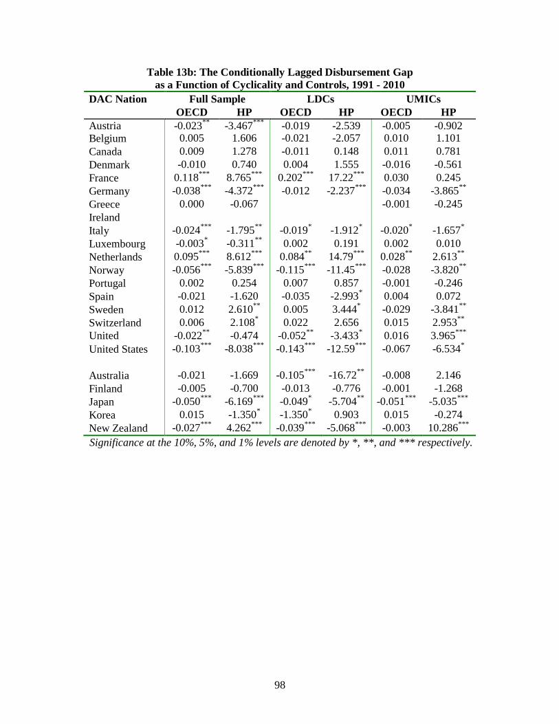
98
Table 13b: The Conditionally Lagged Disbursement Gap
as a Function of Cyclicality and Controls, 1991 - 2010
DAC Nation Full Sample LDCs UMICs
OECD HP OECD HP OECD HP
Austria -0.023**
-3.467***
-0.019 -2.539 -0.005 -0.902
Belgium 0.005 1.606 -0.021 -2.057 0.010 1.101
Canada 0.009 1.278 -0.011 0.148 0.011 0.781
Denmark -0.010 0.740 0.004 1.555 -0.016 -0.561
France 0.118***
8.765***
0.202***
17.22***
0.030 0.245
Germany -0.038***
-4.372***
-0.012 -2.237***
-0.034 -3.865**
Greece 0.000 -0.067 -0.001 -0.245
Ireland
Italy -0.024***
-1.795**
-0.019* -1.912
* -0.020
* -1.657
*
Luxembourg -0.003* -0.311
** 0.002 0.191 0.002 0.010
Netherlands 0.095***
8.612***
0.084**
14.79***
0.028**
2.613**
Norway -0.056***
-5.839***
-0.115***
-11.45***
-0.028 -3.820**
Portugal 0.002 0.254 0.007 0.857 -0.001 -0.246
Spain -0.021 -1.620 -0.035 -2.993* 0.004 0.072
Sweden 0.012 2.610**
0.005 3.444* -0.029 -3.841
**
Switzerland 0.006 2.108* 0.022 2.656 0.015 2.953
**
United
Kingdom
-0.022**
-0.474 -0.052**
-3.433* 0.016 3.965
***
United States -0.103***
-8.038***
-0.143***
-12.59***
-0.067 -6.534*
Australia -0.021 -1.669 -0.105***
-16.72**
-0.008 2.146
Finland -0.005 -0.700 -0.013 -0.776 -0.001 -1.268
Japan -0.050***
-6.169***
-0.049* -5.704
** -0.051
*** -5.035
***
Korea 0.015 -1.350* -1.350
* 0.903 0.015 -0.274
New Zealand -0.027***
4.262***
-0.039***
-5.068***
-0.003 10.286***
Significance at the 10%, 5%, and 1% levels are denoted by *, **, and *** respectively.
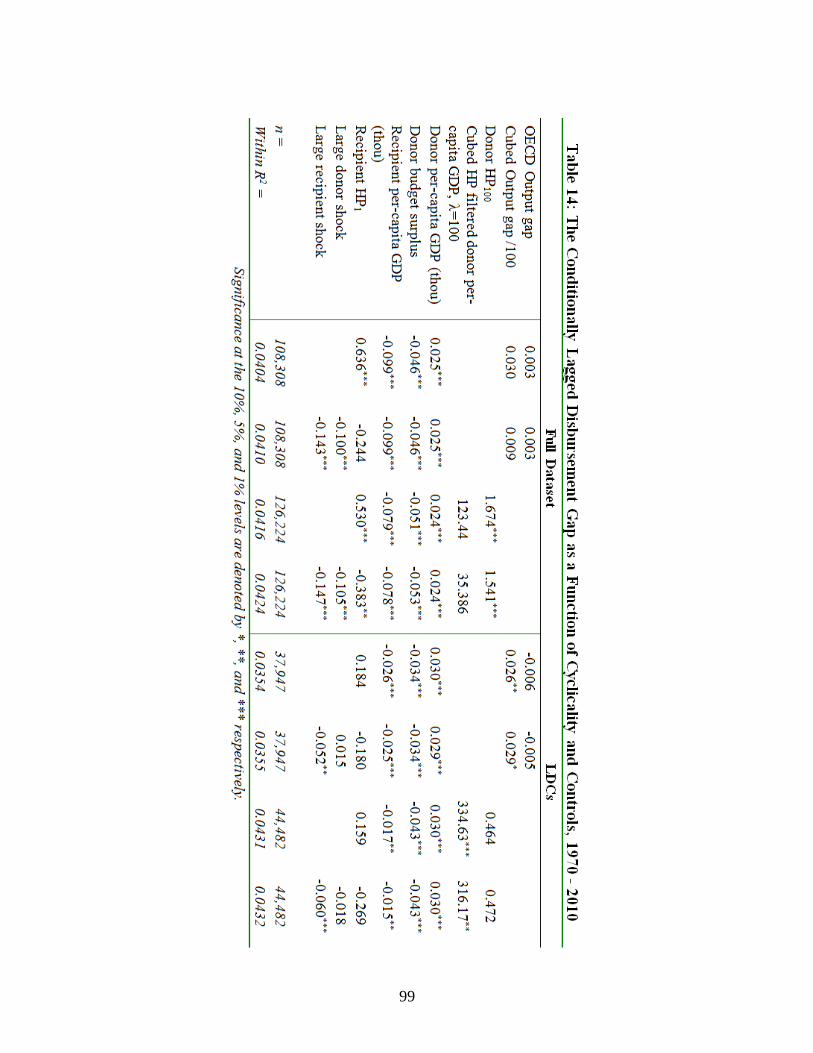
99
100
In Table 14, we see the results of fixed effect regression of donor/recipient pairings across the
entire sample, as was done for the cumulative disbursement gap in Table 11. Using the
conditional lagged cumulative disbursement gap, we see little difference. Nearly all coefficients
show the same sign, significance, and level.
In the more recent subperiod of 1991-2010 there is little change, except for the stronger evidence
of procyclicality of the cumulative disbursement gap. Once the conditional year lag is included,
we can see that the OECD output gap is also highly significantly procyclical across the full
sample, as is the HP cyclicality measure.
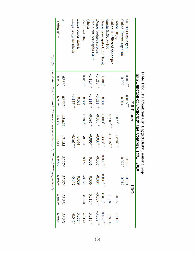
101
102
Finally, the ODA/GNI target of 0.7% is examined for its potential effect on donor behavior. In
1970, this target was largely agreed upon, after suggestion by the Pearson Commission in 1969
and a U.N. resolution in October of 1970. This goal has been reiterated many times since, and so
it is reasonable to expect that donor nations would prefer to demonstrate compliance in bilateral
foreign aid decisions. This measure is reported as the net total disbursements divided by GNI for
each year. It is possible, then, that those nations around the 0.7% mark may demonstrate a
tendency to "stretch" their disbursements beyond what they may otherwise choose, decreasing
the disbursement gap when they are close to the threshold.
To answer this question, the series of ODA/GNI measures were taken for each DAC donor
nation from stats.oecd.org, to be introduced in each of the econometric specifications of Table
14. On average, donor countries continually fail to reach this goal, as the average of this ratio
over all observations is 0.41%. The standard deviation of these observations is 0.26%, with a
minimum of 0.02% (mostly by Korea and Portugal) and a maximum of 1.17% (largely Norway).
If it is true that those near the 0.7% mark tend to stretch their disbursements, then we may begin
by choosing a simple dummy variable to denote those observations where this ratio is near the
mark, such as 5 basis points in either direction. Such a variable was created for those
observations where the ODA/GNI ratio was between 0.65% and 0.75%. There are 2,754
observations within this band, over 20,000 above the band, and over 100,000 below. This
"threshold dummy" variable is shown in Table 15. One potential criticism of using this measure
is that, since the chosen range surrounding 0.7% is near the upper end of the overall range of the
ODA/GNI measure, perhaps there is a simple relationship between the ODA/GNI ratio and the
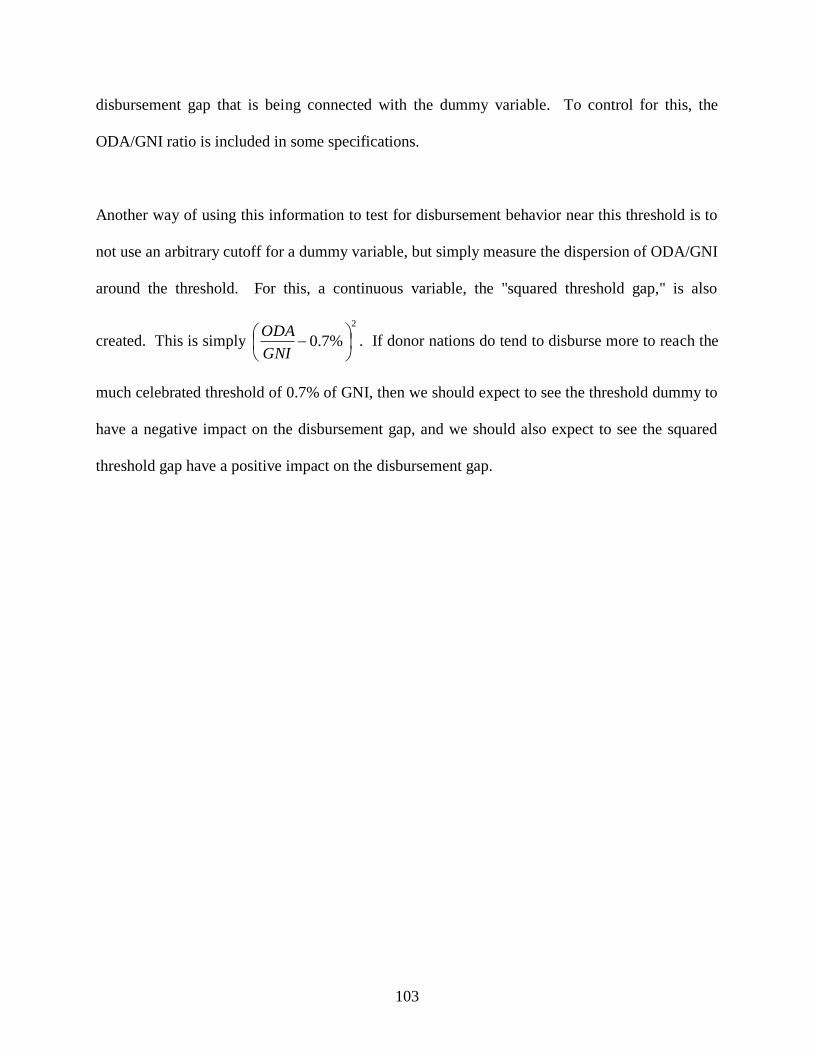
103
disbursement gap that is being connected with the dummy variable. To control for this, the
ODA/GNI ratio is included in some specifications.
Another way of using this information to test for disbursement behavior near this threshold is to
not use an arbitrary cutoff for a dummy variable, but simply measure the dispersion of ODA/GNI
around the threshold. For this, a continuous variable, the "squared threshold gap," is also
created. This is simply
2
%7.0
GNI
ODA. If donor nations do tend to disburse more to reach the
much celebrated threshold of 0.7% of GNI, then we should expect to see the threshold dummy to
have a negative impact on the disbursement gap, and we should also expect to see the squared
threshold gap have a positive impact on the disbursement gap.
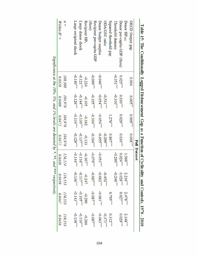
104
105
Table 15 shows the results of these new specifications. It is clear from the coefficients on the
ODA/GNI ratio that the disbursement gap is correlated with smaller levels of ODA as a fraction
of income. This in itself is an interesting relationship, considering that larger levels of ODA
should logically allow for a larger potential gap between commitments and disbursements. We
can see that this is not the case. The threshold dummy shows us that, given the use of the OECD
output gap as our cyclicality measure, those donor nations close to disbursing 0.7% of GNI in
foreign aid do contract their disbursement gap significantly more than those far from this range.
Similar evidence is demonstrated in the coefficients of the squared threshold gap, where nations
giving at greater distances from the 0.7% threshold are significantly more likely to increase, or
fail to decrease, their foreign aid disbursement gap. Clearly this goal, emphasized in the arena of
bilateral aid for more than 40 years, appears to serve as an incentive for more timely ODA
payments.

106

107
Finally, Table 15b is provided for the subperiod of 1991-2010, with the same results as shown in
Table 15 for the full 41-year sample. As before, greater evidence of procyclicality is
demonstrated here relative to the OECD output gap. Again, those donor nations giving a greater
percentage of their GNI to recipients have lower disbursement gaps, and the 0.7% bilateral
foreign aid target continues to appear significant in motivating payment of aid commitments.
2.4 Conclusion
Aid flows continue to appear to be procyclical in nature, although the strength of this relationship
changes with the specific measure chosen. This paper summarizes the disbursement gap and
cumulative disbursement gap, searching for connections between payments of signed bilateral
aid obligations and the business cycle of the donor nation. Multiple tests and specifications
revealed that the disbursement gap was significantly positively related to both standard measures
of the business cycle, both with and without control variables, and with each extension explored.
This relationship appears robust across all donor nations as a set, although counts of individual
donor/recipient pairings do not show the same procyclicality in all specifications.
As research develops surrounding bilateral aid, disbursements, and motivations, evidence
continues to develop that efforts appear to be procyclical in nature, and connected in many ways
more to the donor nation than the recipient nation. The benevolent motivation is hard to justify,
both theoretically and empirically. The present work adds to this growing literature in showing
that, even in the face of a signed commitment of bilateral foreign aid, nations still tend to make
payment decisions based more on their own business cycle and fiscal stance than the apparent
108
needs of recipient nations. Also, the 0.7% of GNI target disbursement ratio appears to affect aid
payments to a much larger degree than the need of recipients.
The reasons to why this empirical regularity exists are likely to be found at pairing-level
analyses. The function describing the cumulative disbursement gap is likely much more
complex than this initial attempt, and may well include the spectrum of conservativism of the
governing parties in donor nations, measures of bureaucratic complexity, key dates regarding the
millennium development goals, etc. This body of knowledge is within the purview of future
research.
109
Chapter 3
The Effect of Cohabitation Exit Costs on Cohabitation, Marriage, and Marriage Hazard
Chapter Summary
Using both the round six and 2006-2008 National Survey of Family Growth (NSFG) data for
both male and female respondents along with macroeconomic data over the same time period, I
test a number of theoretical questions regarding changes in relationship exit costs and their
effects on behavior in cohabitation, marriage, and separation. I find that our proxy for
cohabitation surplus and exit costs significantly affects subsequent decisions of cohabitation,
marriage, separation, and divorce. Also, marriage hazard rates are related to these changing exit
costs in ways consistent with recent advances in theory.

110
3.1 Introduction
Couples dating in high-income countries are increasingly likely to cohabitate prior to marriage.
Traditional mores are quickly giving way to pragmatic, economical living arrangements that
espouse a "try before you buy" attitude regarding marriage. The number of unmarried cohabiting
couples is at record levels; but what is even more significant, perhaps, is the rate of acceleration
in this trend. In fact, while the census bureau estimated 12 million unmarried cohabitors in the
U.S. in its 2005-2007 survey, that number exceeded 13 million in 2009, and reached 15 million
in 2010 (U.S. Census Bureau, 2010). Even these numbers may be understated. It is widely cited
that between 1960 and 2000, unmarried cohabitation grew tenfold (U.S. Census Bureau, 2000).
However, adjustments to survey data performed by Fitch, Goeken, and Ruggles (2005) suggest
that the reported cohabitation rates prior to 1980 are likely overstated, suggesting that this
increase in cohabitation between 1960 and 2000 may more accurately be a 28-fold increase.
Stevenson & Wolfers (2007) provide an excellent summary of the considerable changes in
dynamics of the household in recent years, leading to fewer marriages and divorces, and the
driving forces behind this pervasive acceleration in incidence of cohabitation.
Arguably, cost sharing is part of the reason for this recent surge, and is indeed one focus of this
paper. Theory reasonably suggests that couples are more likely to marry when there are
significant cost savings to do so, and the economic downturn that began in 2006 and has
persisted in recent years has presented couples with attractive incentives to join this trend.
However, this short-run cyclical effect is simultaneous with the long-term trend toward increased
cohabitation which has been noted for decades. With the better information regarding their
potential mate generated by cohabitation, one might expect that marriages formed after
111
premarital cohabitation are more successful than those without. But empirical studies reveal a
persistent "marriage hazard puzzle," as marriages preceded by cohabitation seem subject to
higher divorce rates. Much literature has explored this marriage hazard puzzle (for example, see
Bennett et al., 1988; Axinn & Thornton, 1992; Hall & Zhao, 1995; Brown & Booth, 1996;
Bramlett & Mosher, 2002; and Brien, Lillard, & Stern, 2006). More recent evidence indicates
that, given the right set of control variables, there is empirical support for premarital cohabitation
as a "marriage trial," and that it may actually reduce rates of subsequent divorce (Kulu & Boyle,
2010). Other research focuses on the change in this relationship over time, concluding most
generally that this negative effect of premarital cohabitation on marital success appears to have
weakened in recent decades (Kamp Dush et al., 2003; Hewitt & De Vaus, 2009; Reinhold, 2010).
In summary, the "marriage hazard puzzle" remains an active area of research.
The focus of this paper is not the "trial" motivation for premarital cohabitation, but rather shared
living costs, cohabitation surplus, and other economic influences in relation to cohabitation,
marriage, and separation decisions. The remainder of the paper is organized as follows: In
section 2 recent advancements in theory are explored regarding cohabitation, marriage, and
divorce, empirical work that has been done in concert with that theory, and additional testable
research questions that have been chosen from recent advances in theoretical literature. Section
3 describes the data used in the empirical analysis. In section 4 this dataset is used to test the
theoretical predictions regarding exit costs and relationship decisions that have been introduced.
Section 5 concludes, and discusses limitations to empirical tests that may be addressed by more
complete data in the future.
112
3.2 Relevant Literature and Empirical Questions
The works of Becker may perhaps be considered the starting point for the mainstream branch of
economic theory that includes cohabitation and marriage as a subset. Gains from marriage can
be shown by considering the production of household and market goods. Within this dichotomy,
it is posited that, in a partnership, household goods can be produced more efficiently, and
cooperation may allow the substitutability of time away from household goods and toward
market goods (Becker, 1974). Other explanations of marriage are acknowledged, including love,
desire for children, etc. which are also valid. However, the focus of this paper will remain on
quantifiable, financial gains and from cohabitation and marriage over and above that of a single-
person household.
If we consider the substitutability of time in the production of the necessary household good and
the consumable market good, then, ceteris paribus, a rise in market wages can be shown to
increase the utility of market work, making a cohabitation or marriage arrangement of greater
value (Becker, 1974). It has been shown empirically that, when controlling for years of
schooling, higher-wage individuals tend to marry earlier (Keeley, 1979). There is also evidence
from longitudinal studies that delayed marriage allows career development and wage
enhancement, although later marriages are often formed with partners of lower income levels
(Loughran & Zissimopoulos, 2004). However, the macroeconomic climate is also been shown to
have an inverse relationship to marriage formation. Inflation is positively related to marriage
formation in recent theory, and this is supported empirically (Burdett et. al, 2011). Also,
differential tax treatment also affects cohabitation and marriage decisions; specifically, while the
113
decision to marry seems to be only minimally related to tax code, the decision to progress from
cohabitation to marriage is significantly related (Alm & Whittington, 2003).
It is widely reported in popular press that recessions are associated with increases in
cohabitation. A 2010 Census Bureau report acknowledges that cohabitation increased 13%
between 2009 and 2010, a much faster rate of increase than is the long-run trend, and during
what some term the "great recession" (U.S. Census Bureau, 2010). Additionally, it has been
shown in a European study that co-residential decisions are statistically related to perceived job
insecurity (Becker et. al, 2010) and with poor performance of the labor market (Card & Lemieux,
2000). This is a logical behavioral choice, given the significant economic advantages presented
to cohabitors (Lundberg & Pollak, 2007; Bütikofer & Gerfin, 2009). Given these findings,
perhaps the most basic question to ask is: Do we find evidence that changes in the returns to
shared living expenses (proxied by varied economic environments) increase the likelihood of
cohabitation? If cohabitation is driven, at least partially, by the cost-sharing living arrangement
that accompanies it, then there should be clear empirical data to substantiate this. Many informal
studies present data that worsening economic environments usher in larger numbers of
cohabitating couples, and this is a logical expectation. In this paper, data are explored to
examine this question in the context of recent theoretical advances.
Once a couple cohabits, there is generally a point in time where the couple decides to escalate to
marriage, or to separate. There is some evidence that this "deadline" effect exists. Summary
statistics provided of the 1987-1988 National Survey of Families and Households dataset
indicate that may be approximately two years; less than 40% of cohabitations last that long
114
without proceeding to marriage or ending in separation, and the median cohabitation length at
that time was just 1.3 years (Bumpass & Sweet, 1989). However, other evidence suggests that
the mean lengths of cohabitation have risen from about 2.5 years in the 1980s to 3.5 years around
the year 2000 (United Kingdom Household Longitudinal Study). Further, Kennedy & Bumpass
(2008) use the 1995 and 2002 rounds of the NSFG to determine that average cohabitation length
has increased since the early 1990s, when two-thirds of cohabitations ended within two years,
either in marriage or separation. Their more recent data suggests that only 56% of cohabitations
end within two years, as more couples experience longer cohabitation periods. Still, only one in
ten cohabitations persists after ten years, according to the General Household Survey 1979–2007.
If and when the decision to marry or separate approaches, we should expect exit costs, expense
sharing, etc. to affect this decision. A second empirical question is then: Does a "deadline effect"
exist, and if so, what exogenous factors affect both the deadline effect, and the decision to marry
or separate? Data are utilized to attempt to answer this question as well.
The hazard rate, or divorce rate of couples, is often studied as to contributing factors, including
supposed effects of premarital cohabitation (for example, Axinn & Thornton, 1992; Lillard,
Brien, & Waite, 1995; Kulu & Boyle, 2010). Changes in unemployment levels have specifically
been studied in various contexts, with empirical evidence suggesting that higher unemployment
translates into a job loss within a home, providing a reason for divorce (Jensen and Smith, 1990;
Boheim and Ermisch, 2001; Kraft, 2001; Eliason, 2004). Theoretical justification for this most
commonly involves a simple comparison between expected utility of marriage continuance and
divorce, given a shock to the earnings of one spouse. Charles and Stephens (2004), for example,
115
develop a simple model of marriage where dissolution is assumed to occur whenever the value of
marriage (i.e. surplus above that of being single) drops to a negative value, which occurs with a
job loss. Given this empirical regularity, we expect to see the same in the current dataset.
However, our focus is conditional upon the macroeconomic conditions in which the marriage
was formed. Specifically, a third question is posed: Are marriages formed during poor economic
climates subject to higher hazard rates? That is, if a couple marries in due in part to changes in
monetary incentives, is their marriage more likely to end in divorce? We may expect to see
lower quality matches proceed to marriage in times of economic distress (Farmer & Horowitz
2012), and if this lower expected marriage quality leads to greater divorce rates, we might also
expect to see this third research question answered affirmatively by data, when controlling for
the effects of higher unemployment rates at the time of divorce or separation.
One final test of the importance of exit costs is their effect on decisions to end cohabitation when
a relationship has reached the stage of separation. This end is signaled clearly by divorce for
married couples, even though the cohabitation may be delayed due to economic conditions,
much as the start of cohabitation may similarly affected. This is a growing trend often reported
in popular press29
, but is still a relatively underdeveloped area of study. Many reasons for
choosing to continue cohabitation after divorce as reported in informal sources are similar to
those given for other cohabitation arrangements: cost savings. Expense sharing appears to be a
powerful motivator in causal anecdotal evidence, and so a fourth question is formulated for
further investigation: When divorce is imminent, does cohabitation last significantly longer when
29
There were 37,000 results in a 4/21/12 Google search with the quoted terms "living together
after divorce," and just four results on Google scholar, none dealing with the specific issue of
post-divorce cohabitation by couples.
116
exit costs are higher? While much as been written on divorce, most of the literature does not
distinguish between separation of living quarters and divorce. But if exit costs are higher, we
may expect to see the date of physical separation delayed relative to the date of divorce.
Fortunately, the richness of the chosen cohabitation dataset allows us to test this directly.
3.3 Data
To empirically test the effect of exit costs on cohabitation patterns, multiple datasets were used.
The cohabitation data is from the 2002 (Cycle 6) and 2006-2008 National Survey of Family
Growth (NSFG) surveys, which were designed and administered by the National Center for
Health Statistics (NCHS), in collaboration with other Federal agencies. These were the 6th and
7th such surveys conducted by the NHCS in the past 30 years, and were the first two to have
both male and female datasets. The 2002 survey was conducted from January 2002 to March
2003, and the 2006-2008 survey was conducted from June of 2006 to December of 2008.
Face to face interviews were used to collect data from 14,960 women and 11,063 men all
between the ages of 15 and 45 years of age in the combined two rounds of the survey. The
trained interviewers were all women, who used laptop computers to conduct the interviews. The
interviews lasted an average of about one hour. The date of the interview was captured as a
variable and included in the database. Thousands of variables were captured, including detailed
data regarding pregnancy, sexual activity, childbearing, healthcare, cohabitation, marriage,
divorce, adopted children, and attitudes about these things. Respondents were paid $40 for their
time, and sampling weights were provided to address, among other things, the oversampling of
blacks, Hispanics, and respondents of age 15-24.
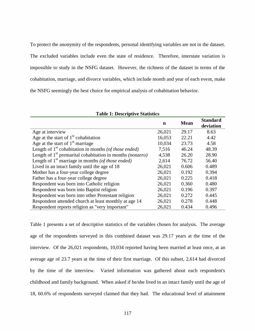
117
To protect the anonymity of the respondents, personal identifying variables are not in the dataset.
The excluded variables include even the state of residence. Therefore, interstate variation is
impossible to study in the NSFG dataset. However, the richness of the dataset in terms of the
cohabitation, marriage, and divorce variables, which include month and year of each event, make
the NSFG seemingly the best choice for empirical analysis of cohabitation behavior.
Table 1: Descriptive Statistics
n Mean Standard
deviation
Age at interview
Age at the start of 1st cohabitation
Age at the start of 1st marriage
Length of 1st cohabitation in months (of those ended)
Length of 1st premarital cohabitation in months (nonzero)
Length of 1st marriage in months (of those ended)
Lived in an intact family until the age of 18
Mother has a four-year college degree
Father has a four-year college degree
Respondent was born into Catholic religion
Respondent was born into Baptist religion
Respondent was born into other Protestant religion
Respondent attended church at least monthly at age 14
Respondent reports religion as "very important"
26,021
16,053
10,034
7,516
4,538
2,614
26,021
26,021
26,021
26,021
26,021
26,021
26,021
26,021
29.17
22.21
23.73
46.24
26.20
76.72
0.606
0.192
0.225
0.360
0.196
0.272
0.278
0.434
8.63
4.42
4.58
48.39
28.90
56.40
0.489
0.394
0.418
0.480
0.397
0.445
0.448
0.496
Table 1 presents a set of descriptive statistics of the variables chosen for analysis. The average
age of the respondents surveyed in this combined dataset was 29.17 years at the time of the
interview. Of the 26,021 respondents, 10,034 reported having been married at least once, at an
average age of 23.7 years at the time of their first marriage. Of this subset, 2,614 had divorced
by the time of the interview. Varied information was gathered about each respondent's
childhood and family background. When asked if he/she lived in an intact family until the age of
18, 60.6% of respondents surveyed claimed that they had. The educational level of attainment

118
by both parents was also recorded, and possession of a four-year college degree was chosen as
the cutoff for an educational attainment binary variable for each parent. 19.2% of respondents'
mothers and 22.5% of respondents' fathers have at least a four-year college degree.
Each respondent reported the religion in which they were raised. The broad categories include
Catholic, Baptist, or other Protestant, and 82.8% of the sample reported one of these as
representative of their childhood religious affiliation. Nearly 28% claimed to have attended
church either once per month, one to three times per month, or every week at the age of fourteen.
Finally, respondents were asked how important religion is in their daily life. Among the choices
of "very important", "somewhat important", and "not important", 43.4% said that their religion is
very important to them.
In exploration of the choices people make in cohabitation, marriage, and divorce, the NSFG
dataset is fairly rich. Each respondent is asked a series of questions about the century month (the
month and year converted to a standard four digit code) in which their first former cohabitation
began, and the century month in which it ended, if so. The respondent provided the same
information for subsequent cohabitations, and also for the starting month of their first marriage,
second marriage, etc. Also, the starting month of their current cohabitation, if applicable, was
collected. From the resulting series of variables, it is possible to ascertain the first cohabitation
by starting date, whether it was premarital or upon marriage. This first cohabital relationship
then either proceeded to marriage, ended in separation, or was in continuation at the time of the
interview. All of this information was captured and formatted in a linear fashion for analysis of
the first cohabitation of each respondent. For example, the starting and ending dates of the jth

119
cohabitation of respondent i are defined as j
iStart and j
iEnd . The age of the respondent j
iSage ,
j
iEage and the unemployment rate j
iSU , j
iEU were also recorded as of these dates, and then the
change in unemployment j
i
j
i
j
i EUSUUchange was calculated.
The average length of first marriages ending by the interview was 6.4 years, whereas the
remaining 7,420 first marriages reported to be in progress had an average age at the time of the
interview of 9.3 years. The average length of first cohabitations ending by the interview was 3.9
years. Cohabitations include marital cohabitation, whether or not the start of cohabitation began
before marriage. The range of these lengths is significant; some cohabitations/marriages ended
in the same month in which they began. The oldest cohabitations/marriages in the current
dataset began in the early 1970s. Half of the more than 16,000 cohabitations in the dataset (2nd
and 3rd quartile by time) began between March of 1989 and February of 2000.
The NSFG dataset contained responses about home ownership, children, and other variables that
could potentially be used to measure exit costs. However, these measures are endogenously
determined, and so cannot be used to measure the effect of an exit cost change. Other measures
of exit costs from outside of this dataset that can be argued as relevant include some relative
earning potential change, as well as any external measure of "re-matching" cost.
The first of these, potential change in earnings/employment prospects, may be proxied by
general economic conditions, measured by macroeconomic indicators such as the national
unemployment level. To include this measure, U.S. nationwide unemployment measures for

120
each month were obtained from The Bureau of Labor Statistics30
. These numbers were matched
with each observation date in the NSFG dataset to create several new variables of the
unemployment rate at each respondent's date of start of cohabitation, end of cohabitation, start of
marriage, separation, and divorce. Over the range of dates reported in this dataset, the U.S.
unemployment rate ranged from 3.8% to 10.8%.
3.4 Exploration of Research Questions
In section 2, four research questions were posed. In this section, these questions are explored
with the current dataset, evaluating any supporting empirical evidence. As mentioned in the
introduction, the marriage hazard puzzle appears to be a robust empirical regularity in a number
of prior analyses. We may first search the current dataset for support of the marriage hazard
puzzle. A simple descriptive table is provided to show survival rates of marriages within the
groups of respondents who married with and without premarital cohabitation.
Table 2: Marriage Survival Rates
n 1 year 2 years 3 years 4 years 5 years
Couples premaritally cohabited
Couples cohabiting at marriage
Difference
3,235
4,353
98.6%
98.3%
0.3%
95.5%
95.3%
0.2%
92.0%
91.9%
0.1%
88.4%
88.4%
0.0%
84.9%
85.5%
-0.6%
This sampling is truncated, using only those who married for the first time at least 5 years prior
to the interview, so that comparable measures of success could be ascertained. With no control
variables, there appears to be no discernible difference between the groups. At five years, there
is only minimal evidence of the marriage hazard puzzle, as a slightly larger percentage of
30
Data were obtained from www.bls.gov; Series ID: LNS14000000.
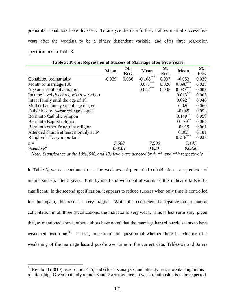
121
premarital cohabitors have divorced. To analyze the data further, I allow marital success five
years after the wedding to be a binary dependent variable, and offer three regression
specifications in Table 3.
Table 3: Probit Regression of Success of Marriage after Five Years
Mean St.
Err. Mean
St.
Err. Mean
St.
Err.
Cohabited premaritally
Month of marriage/100
Age at start of cohabitation
Income level (by categorized variable)
Intact family until the age of 18
Mother has four-year college degree
Father has four-year college degree
Born into Catholic religion
Born into Baptist religion
Born into other Protestant religion
Attended church at least monthly at 14
Religion is "very important"
-0.029 0.036 -0.108***
0.077***
0.042***
0.037
0.026
0.005
-0.053
0.098***
0.037***
0.013**
0.092**
0.020
-0.049
0.140**
-0.129**
-0.019
0.063
0.218***
0.039
0.028
0.005
0.005
0.040
0.060
0.053
0.059
0.064
0.061
0.181
0.038
n =
Pseudo R2
7,588
0.0001
7,588
0.0201
7,147
0.0326
Note: Significance at the 10%, 5%, and 1% levels are denoted by *, **, and *** respectively.
In Table 3, we can continue to see the weakness of premarital cohabitation as a predictor of
marital success after 5 years. Both by itself and with control variables, this indicator fails to be
significant. In the second specification, it appears to reduce success when only time is controlled
for; but again, this result is very fragile. While the coefficient is negative on premarital
cohabitation in all three specifications, the indicator is very weak. This is less surprising, given
that, as mentioned above, other authors have noted that the marriage hazard puzzle seems to have
weakened over time.31
In fact, to explore the question of whether there is evidence of a
weakening of the marriage hazard puzzle over time in the current data, Tables 2a and 3a are
31
Reinhold (2010) uses rounds 4, 5, and 6 for his analysis, and already sees a weakening in this
relationship. Given that only rounds 6 and 7 are used here, a weak relationship is to be expected.
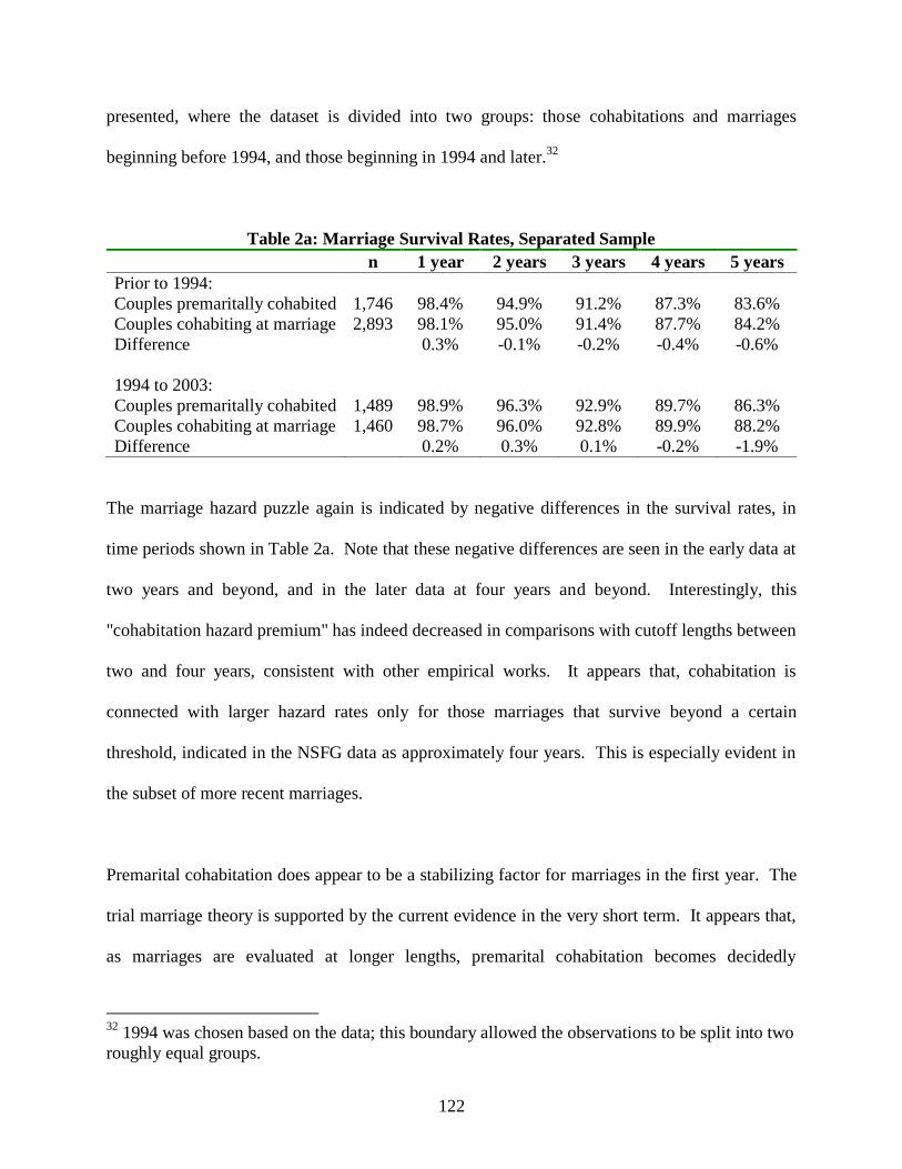
122
presented, where the dataset is divided into two groups: those cohabitations and marriages
beginning before 1994, and those beginning in 1994 and later.32
Table 2a: Marriage Survival Rates, Separated Sample
n 1 year 2 years 3 years 4 years 5 years
Prior to 1994:
Couples premaritally cohabited
Couples cohabiting at marriage
Difference
1994 to 2003:
Couples premaritally cohabited
Couples cohabiting at marriage
Difference
1,746
2,893
1,489
1,460
98.4%
98.1%
0.3%
98.9%
98.7%
0.2%
94.9%
95.0%
-0.1%
96.3%
96.0%
0.3%
91.2%
91.4%
-0.2%
92.9%
92.8%
0.1%
87.3%
87.7%
-0.4%
89.7%
89.9%
-0.2%
83.6%
84.2%
-0.6%
86.3%
88.2%
-1.9%
The marriage hazard puzzle again is indicated by negative differences in the survival rates, in
time periods shown in Table 2a. Note that these negative differences are seen in the early data at
two years and beyond, and in the later data at four years and beyond. Interestingly, this
"cohabitation hazard premium" has indeed decreased in comparisons with cutoff lengths between
two and four years, consistent with other empirical works. It appears that, cohabitation is
connected with larger hazard rates only for those marriages that survive beyond a certain
threshold, indicated in the NSFG data as approximately four years. This is especially evident in
the subset of more recent marriages.
Premarital cohabitation does appear to be a stabilizing factor for marriages in the first year. The
trial marriage theory is supported by the current evidence in the very short term. It appears that,
as marriages are evaluated at longer lengths, premarital cohabitation becomes decidedly
32
1994 was chosen based on the data; this boundary allowed the observations to be split into two
roughly equal groups.
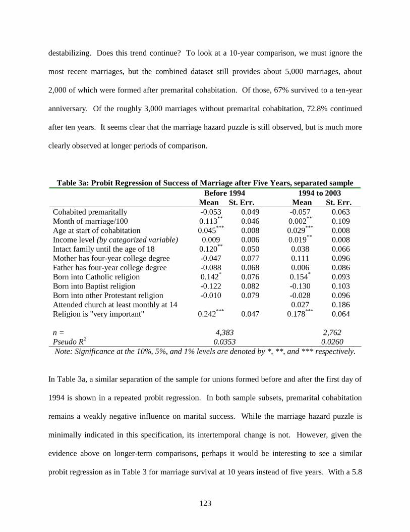
123
destabilizing. Does this trend continue? To look at a 10-year comparison, we must ignore the
most recent marriages, but the combined dataset still provides about 5,000 marriages, about
2,000 of which were formed after premarital cohabitation. Of those, 67% survived to a ten-year
anniversary. Of the roughly 3,000 marriages without premarital cohabitation, 72.8% continued
after ten years. It seems clear that the marriage hazard puzzle is still observed, but is much more
clearly observed at longer periods of comparison.
Table 3a: Probit Regression of Success of Marriage after Five Years, separated sample
Before 1994
Mean St. Err.
1994 to 2003
Mean St. Err.
Cohabited premaritally
Month of marriage/100
Age at start of cohabitation
Income level (by categorized variable)
Intact family until the age of 18
Mother has four-year college degree
Father has four-year college degree
Born into Catholic religion
Born into Baptist religion
Born into other Protestant religion
Attended church at least monthly at 14
Religion is "very important"
-0.053
0.113**
0.045***
0.009
0.120**
-0.047
-0.088
0.142*
-0.122
-0.010
0.242***
0.049
0.046
0.008
0.006
0.050
0.077
0.068
0.076
0.082
0.079
0.047
-0.057
0.002**
0.029***
0.019**
0.038
0.111
0.006
0.154*
-0.130
-0.028
0.027
0.178***
0.063
0.109
0.008
0.008
0.066
0.096
0.086
0.093
0.103
0.096
0.186
0.064
n =
Pseudo R2
4,383
0.0353
2,762
0.0260
Note: Significance at the 10%, 5%, and 1% levels are denoted by *, **, and *** respectively.
In Table 3a, a similar separation of the sample for unions formed before and after the first day of
1994 is shown in a repeated probit regression. In both sample subsets, premarital cohabitation
remains a weakly negative influence on marital success. While the marriage hazard puzzle is
minimally indicated in this specification, its intertemporal change is not. However, given the
evidence above on longer-term comparisons, perhaps it would be interesting to see a similar
probit regression as in Table 3 for marriage survival at 10 years instead of five years. With a 5.8

124
percentage point disparity in survival rates, statistical significance is likely to be found at this
length.
In Table 3b, the marriage hazard puzzle has been identified as statistically evident at a ten-year
comparison. All three specifications show premarital cohabitation to be very highly statistically
significant in predicting marriage hazard after a decade. It is clear now that, at least at some
level, the marriage hazard puzzle persists.
Table 3b: Probit Regression of Success of Marriage after Ten Years
Mean St.
Err. Mean
St.
Err. Mean St. Err.
Cohabited premaritally
Month of marriage/100
Age at start of cohabitation
Income level (by categorized variable)
Intact family until the age of 18
Mother has four-year college degree
Father has four-year college degree
Born into Catholic religion
Born into Baptist religion
Born into other Protestant religion
Religion is "very important"
-0.165***
0.037 -0.258***
0.095***
0.058***
0.039
0.033
0.006
-0.194***
0.117***
0.052***
0.011**
0.151***
-0.152**
0.046
0.089
-0.190***
-0.066
0.271***
0.040
0.034
0.006
0.005
0.042
0.063
0.057
0.063
0.070
0.066
0.040
n =
Pseudo R2
5,226
0.0031
5,226
0.0303
4,935
0.0470
Note: Significance at the 10%, 5%, and 1% levels are denoted by *, **, and *** respectively.
It is noteworthy that, although this is the most recent data available from the NSFG studies, the
marriages constituting the data in Table 3b are not as recent as the reader may assume. The data
was gathered from interviews from 2002 to 2008, and these marriages are all at least 10 years of
age. This means that even the most recent marriage represented in the table began as early as
1998. In fact, the range of starting months for the marriages represented in Table 3b spans over
26 years, from July of 1972 to December of 1998. The mean starting month is September of
1988.

125
Future studies will be able to inform us of changes to the marriage hazard puzzle, and if the
effects of cohabitation continue to weaken in predicting divorce. Again, the main focus of this
paper is on exit costs and their effects. We may now begin addressing the first of four theoretical
questions of cohabitation patterns.
Question #1: Do we find evidence that changes in the returns to shared living expenses (proxied
by varied economic environments) increase the likelihood of cohabitation?
Shared living expenses are a significant financial benefit for couples, and much theory on
cohabitation assumes that this may be a driver in couples choosing to cohabitate, or at least affect
the timing of cohabitation. Using the current datasets, simple regressions may be run,
considering the unemployment level an exogenous proxy for cohabitation surplus, as greater
unemployment levels are correlated with lower household income, and greater uncertainty
regarding income flows. As such, I start with a simple probit regression equation:
(1) 1Cohab
Cohab, or the incidence of premarital cohabitation as a binary variable, provides us some initial
insight as to what factors affect cohabitation. It is expected that higher levels of unemployment
encourage cohabitation, as this is regularly observed. The omega vector of respondent
characteristics may offer additional information on the sample group.
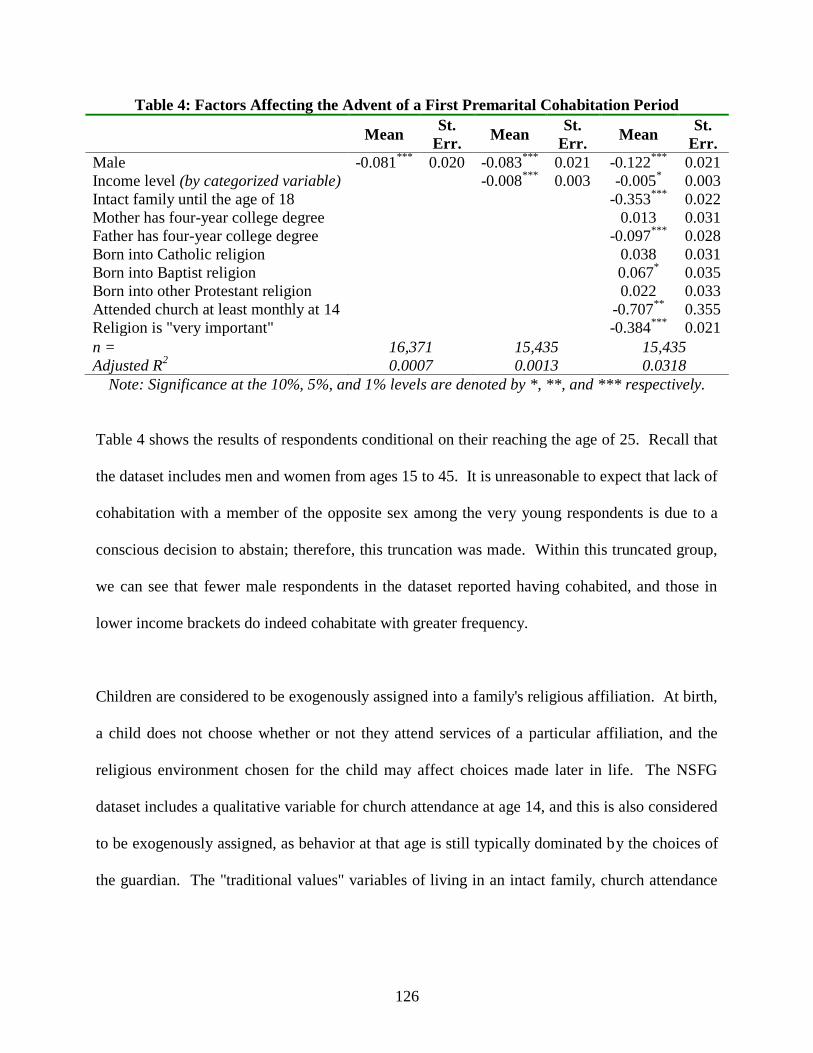
126
Table 4: Factors Affecting the Advent of a First Premarital Cohabitation Period
Mean St.
Err. Mean
St.
Err. Mean
St.
Err.
Male
Income level (by categorized variable)
Intact family until the age of 18
Mother has four-year college degree
Father has four-year college degree
Born into Catholic religion
Born into Baptist religion
Born into other Protestant religion
Attended church at least monthly at 14
Religion is "very important"
-0.081***
0.020 -0.083***
-0.008***
0.021
0.003
-0.122***
-0.005*
-0.353***
0.013
-0.097***
0.038
0.067*
0.022
-0.707**
-0.384***
0.021
0.003
0.022
0.031
0.028
0.031
0.035
0.033
0.355
0.021
n =
Adjusted R2
16,371
0.0007
15,435
0.0013
15,435
0.0318
Note: Significance at the 10%, 5%, and 1% levels are denoted by *, **, and *** respectively.
Table 4 shows the results of respondents conditional on their reaching the age of 25. Recall that
the dataset includes men and women from ages 15 to 45. It is unreasonable to expect that lack of
cohabitation with a member of the opposite sex among the very young respondents is due to a
conscious decision to abstain; therefore, this truncation was made. Within this truncated group,
we can see that fewer male respondents in the dataset reported having cohabited, and those in
lower income brackets do indeed cohabitate with greater frequency.
Children are considered to be exogenously assigned into a family's religious affiliation. At birth,
a child does not choose whether or not they attend services of a particular affiliation, and the
religious environment chosen for the child may affect choices made later in life. The NSFG
dataset includes a qualitative variable for church attendance at age 14, and this is also considered
to be exogenously assigned, as behavior at that age is still typically dominated by the choices of
the guardian. The "traditional values" variables of living in an intact family, church attendance
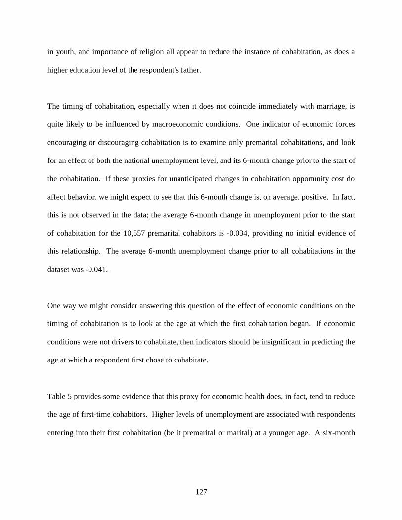
127
in youth, and importance of religion all appear to reduce the instance of cohabitation, as does a
higher education level of the respondent's father.
The timing of cohabitation, especially when it does not coincide immediately with marriage, is
quite likely to be influenced by macroeconomic conditions. One indicator of economic forces
encouraging or discouraging cohabitation is to examine only premarital cohabitations, and look
for an effect of both the national unemployment level, and its 6-month change prior to the start of
the cohabitation. If these proxies for unanticipated changes in cohabitation opportunity cost do
affect behavior, we might expect to see that this 6-month change is, on average, positive. In fact,
this is not observed in the data; the average 6-month change in unemployment prior to the start
of cohabitation for the 10,557 premarital cohabitors is -0.034, providing no initial evidence of
this relationship. The average 6-month unemployment change prior to all cohabitations in the
dataset was -0.041.
One way we might consider answering this question of the effect of economic conditions on the
timing of cohabitation is to look at the age at which the first cohabitation began. If economic
conditions were not drivers to cohabitate, then indicators should be insignificant in predicting the
age at which a respondent first chose to cohabitate.
Table 5 provides some evidence that this proxy for economic health does, in fact, tend to reduce
the age of first-time cohabitors. Higher levels of unemployment are associated with respondents
entering into their first cohabitation (be it premarital or marital) at a younger age. A six-month
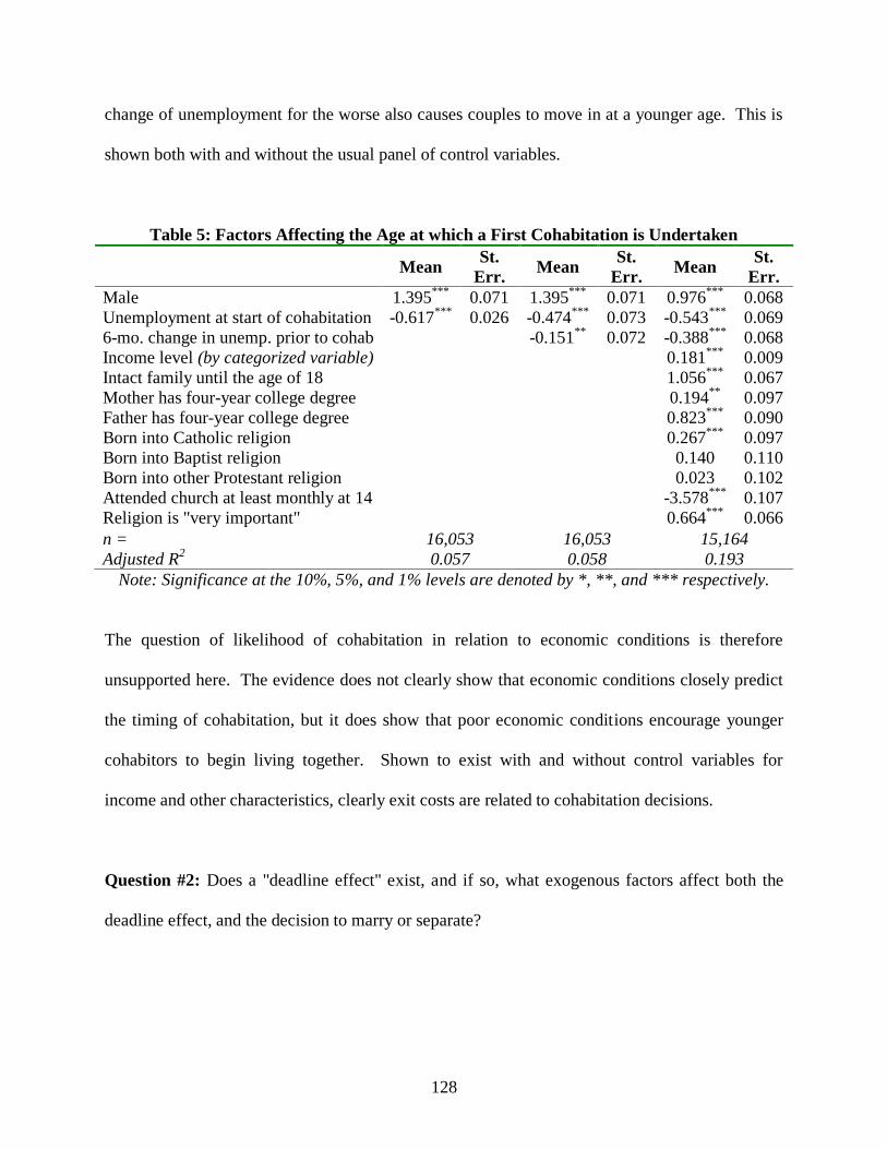
128
change of unemployment for the worse also causes couples to move in at a younger age. This is
shown both with and without the usual panel of control variables.
Table 5: Factors Affecting the Age at which a First Cohabitation is Undertaken
Mean St.
Err. Mean
St.
Err. Mean
St.
Err.
Male
Unemployment at start of cohabitation
6-mo. change in unemp. prior to cohab
Income level (by categorized variable)
Intact family until the age of 18
Mother has four-year college degree
Father has four-year college degree
Born into Catholic religion
Born into Baptist religion
Born into other Protestant religion
Attended church at least monthly at 14
Religion is "very important"
1.395***
-0.617***
0.071
0.026
1.395***
-0.474***
-0.151**
0.071
0.073
0.072
0.976***
-0.543***
-0.388***
0.181***
1.056***
0.194**
0.823***
0.267***
0.140
0.023
-3.578***
0.664***
0.068
0.069
0.068
0.009
0.067
0.097
0.090
0.097
0.110
0.102
0.107
0.066
n =
Adjusted R2
16,053
0.057
16,053
0.058
15,164
0.193
Note: Significance at the 10%, 5%, and 1% levels are denoted by *, **, and *** respectively.
The question of likelihood of cohabitation in relation to economic conditions is therefore
unsupported here. The evidence does not clearly show that economic conditions closely predict
the timing of cohabitation, but it does show that poor economic conditions encourage younger
cohabitors to begin living together. Shown to exist with and without control variables for
income and other characteristics, clearly exit costs are related to cohabitation decisions.
Question #2: Does a "deadline effect" exist, and if so, what exogenous factors affect both the
deadline effect, and the decision to marry or separate?
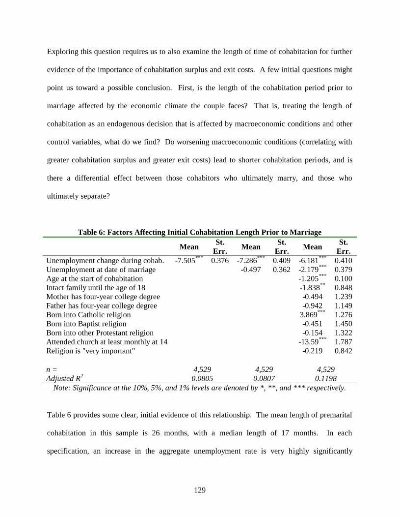
129
Exploring this question requires us to also examine the length of time of cohabitation for further
evidence of the importance of cohabitation surplus and exit costs. A few initial questions might
point us toward a possible conclusion. First, is the length of the cohabitation period prior to
marriage affected by the economic climate the couple faces? That is, treating the length of
cohabitation as an endogenous decision that is affected by macroeconomic conditions and other
control variables, what do we find? Do worsening macroeconomic conditions (correlating with
greater cohabitation surplus and greater exit costs) lead to shorter cohabitation periods, and is
there a differential effect between those cohabitors who ultimately marry, and those who
ultimately separate?
Table 6: Factors Affecting Initial Cohabitation Length Prior to Marriage
Mean St.
Err. Mean
St.
Err. Mean
St.
Err.
Unemployment change during cohab.
Unemployment at date of marriage
Age at the start of cohabitation
Intact family until the age of 18
Mother has four-year college degree
Father has four-year college degree
Born into Catholic religion
Born into Baptist religion
Born into other Protestant religion
Attended church at least monthly at 14
Religion is "very important"
-7.505***
0.376 -7.286***
-0.497
0.409
0.362
-6.181***
-2.179***
-1.205***
-1.838**
-0.494
-0.942
3.869***
-0.451
-0.154
-13.59***
-0.219
0.410
0.379
0.100
0.848
1.239
1.149
1.276
1.450
1.322
1.787
0.842
n =
Adjusted R2
4,529
0.0805
4,529
0.0807
4,529
0.1198
Note: Significance at the 10%, 5%, and 1% levels are denoted by *, **, and *** respectively.
Table 6 provides some clear, initial evidence of this relationship. The mean length of premarital
cohabitation in this sample is 26 months, with a median length of 17 months. In each
specification, an increase in the aggregate unemployment rate is very highly significantly
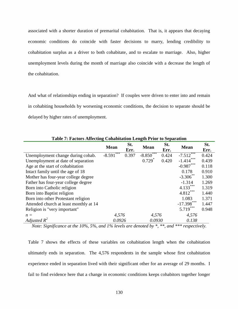
130
associated with a shorter duration of premarital cohabitation. That is, it appears that decaying
economic conditions do coincide with faster decisions to marry, lending credibility to
cohabitation surplus as a driver to both cohabitate, and to escalate to marriage. Also, higher
unemployment levels during the month of marriage also coincide with a decrease the length of
the cohabitation.
And what of relationships ending in separation? If couples were driven to enter into and remain
in cohabiting households by worsening economic conditions, the decision to separate should be
delayed by higher rates of unemployment.
Table 7: Factors Affecting Cohabitation Length Prior to Separation
Mean St.
Err. Mean
St.
Err. Mean
St.
Err.
Unemployment change during cohab.
Unemployment at date of separation
Age at the start of cohabitation
Intact family until the age of 18
Mother has four-year college degree
Father has four-year college degree
Born into Catholic religion
Born into Baptist religion
Born into other Protestant religion
Attended church at least monthly at 14
Religion is "very important"
-8.591***
0.397 -8.850***
0.729*
0.424
0.420
-7.512***
-1.414***
-0.987***
0.178
-3.306**
-1.314
4.133***
4.812***
1.083
-17.398***
5.719***
0.424
0.439
0.118
0.910
1.300
1.269
1.319
1.440
1.371
1.447
0.948
n =
Adjusted R2
4,576
0.0926
4,576
0.0930
4,576
0.138
Note: Significance at the 10%, 5%, and 1% levels are denoted by *, **, and *** respectively.
Table 7 shows the effects of these variables on cohabitation length when the cohabitation
ultimately ends in separation. The 4,576 respondents in the sample whose first cohabitation
experience ended in separation lived with their significant other for an average of 29 months. I
fail to find evidence here that a change in economic conditions keeps cohabitors together longer

131
when they are bound to separate. Conversely, a worsening economic climate is shown here to
decrease the length of nonmarital cohabitation as in the case of those who eventually married.
While this is inconsistent with exit costs as drivers of cohabitation, it is consistent with theory
discussed in the introduction, suggesting that a shock of unemployment within a household
causes divorce, as the utility of marriage has fallen dramatically for one of the agents. Perhaps
this effect is also seen in premarital cohabitations, and is the dominating effect in this data.
A more direct way of exploring this question is to look at the decision point itself. One assertion
by Farmer & Horowitz (2012) is that an exogenous increase in exit costs will, all else equal,
cause cohabitors to be more likely to marry, accepting (on average) a lower quality draw, which
will therefore increase marriage hazard in the long run. With the current dataset and a proxy
variable for exit costs, we can come very close to directly testing this theory. Given an economic
environment at the time of first cohabitation, I again take the change in unemployment to proxy
for an exogenous shock to exit costs, and see if evidence suggests that increase in marriage
incidence tends to follow worsening economic conditions, and whether those marriages are more
likely to fail.
A probit regression for only those respondents entering into a first cohabitation that has either
evolved to marriage or ended in separation will allow each of these decisions to be evaluated
simultaneously with the same list of control variables. If worsening economic conditions,
manifesting as potentially greater cost savings for cohabitors and greater costs for those who
split, are legitimate factors affecting these decisions, we should expect such an analysis to show
itself clearly in this model.
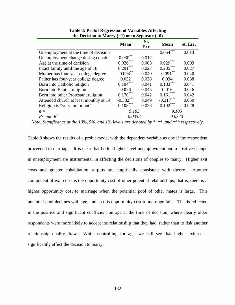
132
Table 8: Probit Regression of Variables Affecting
the Decision to Marry (=1) or to Separate (=0)
Mean St.
Err. Mean St. Err.
Unemployment at the time of decision
Unemployment change during cohab.
Age at the time of decision
Intact family until the age of 18
Mother has four-year college degree
Father has four-year college degree
Born into Catholic religion
Born into Baptist religion
Born into other Protestant religion
Attended church at least monthly at 14
Religion is "very important"
0.030**
0.026***
0.291***
-0.094**
0.032
0.194***
0.026
0.170***
-0.382***
0.108***
0.012
0.003
0.027
0.040
0.038
0.041
0.045
0.042
0.049
0.028
0.054***
0.029***
0.285***
-0.091**
0.034
0.183***
0.016
0.161***
-0.317***
0.102***
0.013
0.003
0.027
0.040
0.038
0.041
0.046
0.042
0.050
0.028
n =
Pseudo R2
9,105
0.0332
9,105
0.0343
Note: Significance at the 10%, 5%, and 1% levels are denoted by *, **, and *** respectively.
Table 8 shows the results of a probit model with the dependent variable as one if the respondent
proceeded to marriage. It is clear that both a higher level unemployment and a positive change
in unemployment are instrumental in affecting the decisions of couples to marry. Higher exit
costs and greater cohabitation surplus are empirically consistent with theory. Another
component of exit costs is the opportunity cost of other potential relationships; that is, there is a
higher opportunity cost to marriage when the potential pool of other mates is large. This
potential pool declines with age, and so this opportunity cost to marriage falls. This is reflected
in the positive and significant coefficient on age at the time of decision, where clearly older
respondents were more likely to accept the relationship that they had, rather than to risk another
relationship quality draw. While controlling for age, we still see that higher exit costs
significantly affect the decision to marry.

133
Question #3: Are marriages formed during poor economic climates subject to higher hazard
rates?
There are certain limitations to using the current dataset to answer this question. The oldest
respondent is only 45 years of age, and the average length of first marriages that end in divorce is
somewhere from about 8 years (http://www.census.gov/prod/2005pubs/ p70-97.pdf) to about 11
years (http://www.divorceinfo.com/statistics.htm). It can be problematic to rely on the length of
marriage as an indicator of success, but we can at least compare the CDFs of divorces in the
datasets for marriages borne out of various economic environments.
In the current dataset of over 26,000 respondents, 10,034 have married, and 2,614 have already
seen that first marriage end. Those 10,034 marriages began on average 10.86 years prior to the
interview. The remaining 7,420 respondents who had remained married to their first spouse had,
at the time of the interview, been married an average of 9.27 years.
A total of 7,588 marriages occurred at least 5 years prior to the time of the interview, 5,266
marriages occurred at least 10 years prior to the time of the interview, and 2,848 marriages
occurred at least 15 years prior to the time of the interview. In each of these three subgroups, a
probit of the incidence of divorce is explored to see to what degree economic conditions and
other control variables affected this decision.

134
Table 9: Probit of Divorce at Various Thresholds of Marriage Age
Minimum length of marriage
at time of interview 5 years
Mean St. Err.
10 years
Mean St. Err.
15 years
Mean St. Err.
Unemployment at start of cohabitation
Unemployment at the time of separation
Age at the time of marriage
Income level (by categorized variable)
Intact family until the age of 18
Mother has four-year college degree
Father has four-year college degree
Born into Catholic religion
Born into Baptist religion
Born into other Protestant religion
Attended church at least monthly at 14
Religion is "very important"
0.147***
0.096***
-0.018*
0.085***
0.117
0.090
0.175
-0.044
0.077
0.192
-0.454
-0.120*
0.029
0.033
0.009
0.010
0.071
0.120
0.113
0.110
0.118
0.120
0.325
0.072
0.081**
0.120***
-0.012
0.081***
0.024
0.115
0.121
0.008
0.143
0.287**
-0.145*
0.035
0.036
0.012
0.011
0.085
0.147
0.134
0.130
0.141
0.144
0.085
0.069
0.108**
-0.040**
0.081***
0.093
0.045
0.345*
0.033
0.426**
0.415**
-0.134
0.042
0.044
0.019
0.015
0.111
0.191
0.204
0.164
0.183
0.187
0.111
n =
Pseudo R2
2,645
0.1002
2,132
0.0824
1,393
0.0987
Note: Significance at the 10%, 5%, and 1% levels are denoted by *, **, and *** respectively.
Note: Church attendance at age 14 was omitted from two regressions due to collinearity.
In all three selections of marriage lengths, there is a positive relationship between poor economic
conditions at the start of cohabitation and ultimate divorce. This is consistent with recent
advances in theory, suggesting that higher exit costs directly affect the decision of couples to
escalate from dating to cohabitation to marriage (or directly to marriage), encouraging marriages
that are of lower match quality. This increases the likelihood that such marriages will end in
divorce, as these data directly confirm. Importantly, this is shown with the inclusion of a control
variable for unemployment at the time of separation. Again, the effect of marriage utility being
shocked by unemployment suggests that higher unemployment is a driver to separate, which is
demonstrated by the positive and significant relationship between unemployment at separation
and divorce. With this control in place, the separate effect of a poor economic condition at the
time of cohabitation is shown separately as an ultimate driver of divorce.
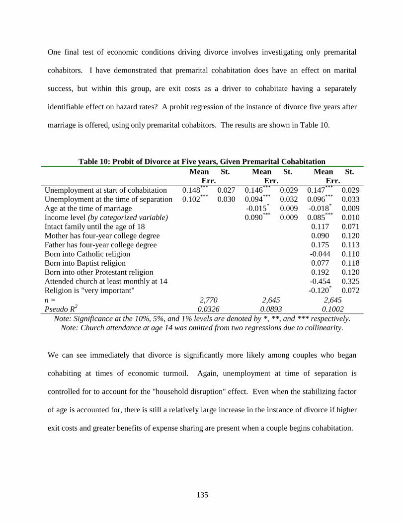
135
One final test of economic conditions driving divorce involves investigating only premarital
cohabitors. I have demonstrated that premarital cohabitation does have an effect on marital
success, but within this group, are exit costs as a driver to cohabitate having a separately
identifiable effect on hazard rates? A probit regression of the instance of divorce five years after
marriage is offered, using only premarital cohabitors. The results are shown in Table 10.
Table 10: Probit of Divorce at Five years, Given Premarital Cohabitation
Mean St.
Err.
Mean St.
Err.
Mean St.
Err.
Unemployment at start of cohabitation
Unemployment at the time of separation
Age at the time of marriage
Income level (by categorized variable)
Intact family until the age of 18
Mother has four-year college degree
Father has four-year college degree
Born into Catholic religion
Born into Baptist religion
Born into other Protestant religion
Attended church at least monthly at 14
Religion is "very important"
0.148***
0.102***
0.027
0.030
0.146***
0.094***
-0.015*
0.090***
0.029
0.032
0.009
0.009
0.147***
0.096***
-0.018*
0.085***
0.117
0.090
0.175
-0.044
0.077
0.192
-0.454
-0.120*
0.029
0.033
0.009
0.010
0.071
0.120
0.113
0.110
0.118
0.120
0.325
0.072
n =
Pseudo R2
2,770
0.0326
2,645
0.0893
2,645
0.1002
Note: Significance at the 10%, 5%, and 1% levels are denoted by *, **, and *** respectively.
Note: Church attendance at age 14 was omitted from two regressions due to collinearity.
We can see immediately that divorce is significantly more likely among couples who began
cohabiting at times of economic turmoil. Again, unemployment at time of separation is
controlled for to account for the "household disruption" effect. Even when the stabilizing factor
of age is accounted for, there is still a relatively large increase in the instance of divorce if higher
exit costs and greater benefits of expense sharing are present when a couple begins cohabitation.
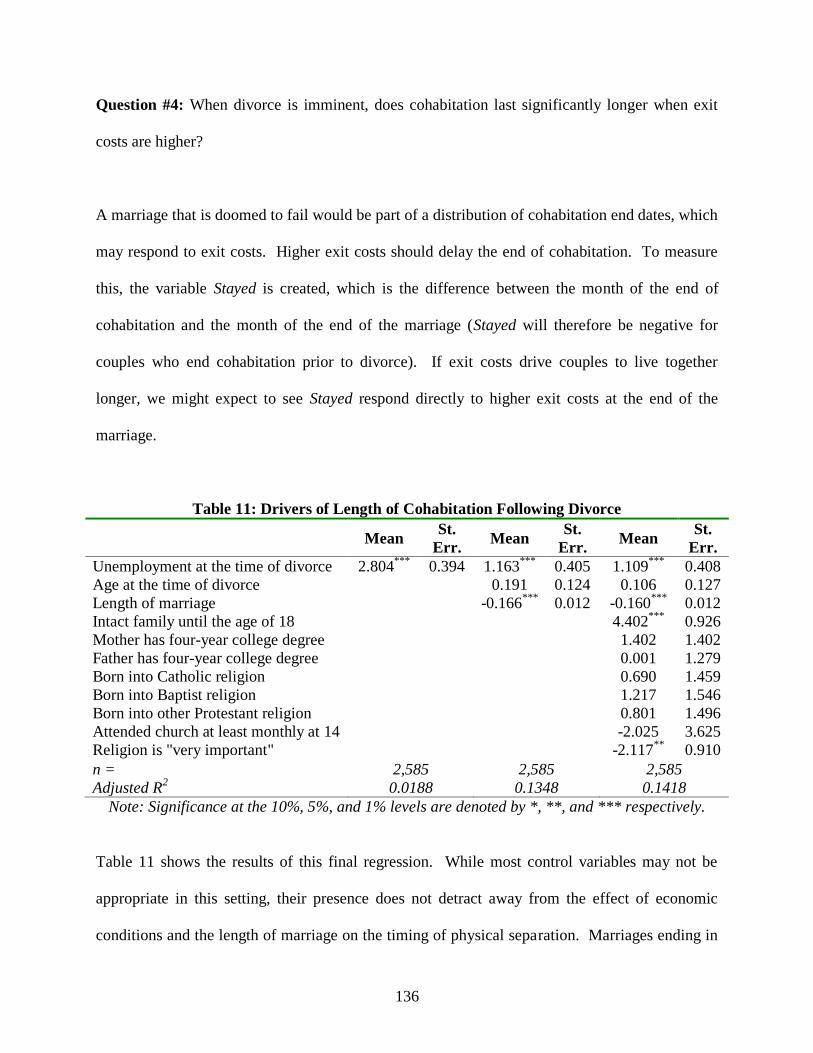
136
Question #4: When divorce is imminent, does cohabitation last significantly longer when exit
costs are higher?
A marriage that is doomed to fail would be part of a distribution of cohabitation end dates, which
may respond to exit costs. Higher exit costs should delay the end of cohabitation. To measure
this, the variable Stayed is created, which is the difference between the month of the end of
cohabitation and the month of the end of the marriage (Stayed will therefore be negative for
couples who end cohabitation prior to divorce). If exit costs drive couples to live together
longer, we might expect to see Stayed respond directly to higher exit costs at the end of the
marriage.
Table 11: Drivers of Length of Cohabitation Following Divorce
Mean St.
Err. Mean
St.
Err. Mean
St.
Err.
Unemployment at the time of divorce
Age at the time of divorce
Length of marriage
Intact family until the age of 18
Mother has four-year college degree
Father has four-year college degree
Born into Catholic religion
Born into Baptist religion
Born into other Protestant religion
Attended church at least monthly at 14
Religion is "very important"
2.804***
0.394 1.163***
0.191
-0.166***
0.405
0.124
0.012
1.109***
0.106
-0.160***
4.402***
1.402
0.001
0.690
1.217
0.801
-2.025
-2.117**
0.408
0.127
0.012
0.926
1.402
1.279
1.459
1.546
1.496
3.625
0.910
n =
Adjusted R2
2,585
0.0188
2,585
0.1348
2,585
0.1418
Note: Significance at the 10%, 5%, and 1% levels are denoted by *, **, and *** respectively.
Table 11 shows the results of this final regression. While most control variables may not be
appropriate in this setting, their presence does not detract away from the effect of economic
conditions and the length of marriage on the timing of physical separation. Marriages ending in

137
times of macroeconomic hardship see cohabitors living together longer than those couples
separating in better times. Shorter marriages are also shown to be associated with delayed
physical separation.
However, as with other analyses, there may well be other stories being told in the data that
pervade. For instance, if worsening economic conditions are the cause of added stress, job
changes, etc. that precipitate a move by one of the cohabitors, it may affect cohabitation surplus.
This is especially true considering that a proxy is used for this surplus. Nonetheless, these data
show that post-divorce cohabitation tends to show agreement between theory and empirics.
3.5 Conclusion
A recent theoretical paper has drawn attention to the potential role of exit costs in decisions to
cohabitate, marry, and separate. This paper uses changing unemployment rates as a broad proxy
of changes in exit costs to test empirically some of the theoretical claims put forth. I find that
exit costs have a significant effect on decisions to cohabitate, marry, separate, and divorce.
The regularity of the marriage hazard puzzle is obscured in the current dataset for short-term
marriages. Much stronger evidence of this puzzle is found with an examination of marital
success at the 10-year mark. Other authors have already noted the decline of this effect in more
recent years, so the obscurity of the puzzle in the most recent marriages may indeed be a
continuation of this trend.

138
The first question was whether we find evidence that changes in economic conditions affect the
advent of cohabitation. Changing economic conditions can affect union incentive through many
channels, including expense sharing in cohabitation (whether marital or not), downside risk,
diversification benefits, etc. Using U.S. unemployment data as the proxy for changes in
economic gains to cohabitation, there is strong evidence that worsening economic conditions do
influence the timing of cohabitation and marriage. Higher risk of job loss does appear to provide
incentive for union formation, or forming them perhaps more quickly.
Secondly, I explored whether exit costs significantly affect the choice of marriage or exit, once a
couple reaches one of those decisions. The length of cohabitation prior to marriage or separation
was examined first, and a greater exit cost proxy was shown to reduce the length of premarital
cohabitation, hurrying the couple along to marriage. Paradoxically, an increase in exit costs over
the course of the cohabitation also seemed to shorten the cohabitation length for couples that
finally separated. But the choice to marry or separate was also examined in Table 8, where an
increase in exit costs was clearly associated with the decision to marry rather than to separate.
Next, since exit costs do tend to push couples together in more economical living arrangements,
including into marriage, what can we say about the relative strength of such marriages? Are
such marriages formed in these times of economic decline more subject to subsequent divorce?
Yes. In multiple groups, it appears clear that our exit cost proxy is related to divorce rates in a
predictable fashion. It is quite possible from the data that these marriages tend to provide lower
utility to the pair, as marriages formed at times of pressure from higher exit costs are more likely

139
to eventually fail. Also, a separate analysis of only premarital cohabitors showed that unions
formed in poor economic climates are also more likely to end in separation.
Finally, when divorce is imminent, cohabitations tend to last longer when exit costs are higher.
This is shown with a generated variable of the number of months cohabitation of a couple lasts
beyond the month in which they divorce. Interestingly, the length of the marriage is negatively
correlated with this variable.
Throughout these analyses, control variables tell us of other interesting relationships that exist in
the data. Clearly a person's tendency to premaritally cohabitate, to marry, to separate, or to
divorce, is influenced by the relationships that have been modeled to them by their parents, by
religious affiliation, and a host of unobservable variables that remain unexplored. Herein, exit
costs, as proxied by U.S. national unemployment levels and changes, have been used as a
correlate guide to the effect that exit costs may have on these decisions.
One limitation of empirical work at this point is that a more direct and composite measure of exit
costs remains unavailable. It is unclear as to what the "best" measure of exit cost would be, as it
can be interpreted as such a multifaceted concept as to defy practical measure. Exit costs could
be considered a measure of living costs, moving costs, transaction costs, psychological stresses,
opportunity costs regarding other potential mates, matching costs, social pressures, etc. We are
far from constructing such a measure. Marital satisfaction and utility are also missing variables
in the NSFG dataset; and so, such implications of theory with regard to that are not testable.
Even if that variable was collected, it would be arguably weakened by the fact that satisfaction is
140
known to change over the course of the relationship. Limitations to empirical tests that may be
addressed by more complete data in the future. With these thoughts in mind, future research may
be enhanced by survey modules in longitudinal surveys directly designed to measure several
dimensions of exit costs.
141
References
Alesina, Alberto & David Dollar. 2000. "Who gives foreign aid to whom and why? Journal of
Economic Growth, 5(1): pp. 33-63
Alesina, Alberto & Beatrice Weber. 1999. "Do Corrupt Governments Receive Less Foreign
Aid?" NBER Working Paper No. 7108
Alm, James & Leslie A. Whittington. 2003. "Shacking Up or Shelling Out: Income Taxes,
Marriage, and Cohabitation," Review of Economics of the Household, Volume 1, Number 3
(2003), pp. 169-186
Amendariz, B. & Morduch, J. 2000. "Microfinance Beyond Group Lending", Economics of
Transition, Volume 8, Issue 2, pp. 401-420
Arndt, C., S. Jones, & F. Tarp. 2010. "Aid and growth: Have we come full circle?" University
of Copenhagen Department of Economics and UNU-WIDER, unpublished manuscript
(Copenhagen: University of Copenhagen; Helsinki: UNU-WIDER)
Arun, Thankom, & David Hulme. 2008. "Microfinance - A Way Forward", Working Paper 54,
Brooks World Poverty Institute, The University of Manchester
Axinn W.G. & A. Thornton. 1992. "The relationship between cohabitation and divorce:
Selectivity or causality?" Demography. 29(3), pp. 357–374
Backus, David K. & Patrick J. Kehoe. 1992. "International Evidence on the Historical
Properties of Business Cycles," The American Economic Review, Vol. 82, No. 4, pp. 864-888
Basu, S. 2004. "Securitization and the Challenges Faced in Micro Finance",
www.iciciresearchcentre.org
Becker, Gary S. 1974. "A Theory of Marriage, Part I", in: T. W. Schultz, ed., Economics of the
family. Chicago: University of Chicago Press, pp. 293-344.
Becker, Sascha O., Samuel Bentolila, Ana Fernandes, & Andrea Ichino. 2010. "Youth
Emanciapation and Perceived Job Insecurity of Parents and Children," Journal of Population
Economics," Volume 23, Number 3 (2010), pp. 1047-1071
Beffy, P.-O., P. Ollivaud, P. Richardson, & F. Sedillot. 2006. “New OECD methods for supply-
side and medium-term assessment: A capital services approach,” OECD Working Paper No. 482
(Paris: Organization for Economic Cooperation & Development)
Bennett, Neil G., Ann Klimas Blanc, & David E. Bloom. 1988. “Commitment and the Modern
Union: Assessing the Link Between Premarital Cohabitation and Subsequent Marital Stability,”
American Sociological Review, Vol. 53, No. 1 (Feb.), pp. 127-138.

142
Berthelemy, Jean-Claude. 2006. "Aid allocation: Comparing donors’ behaviours," Swedish
Economic Policy Review, 13, pp. 75-109
Berthelemy, Jean-Claude & Ariane Tichit. 2004. "Bilateral donors' aid allocation decisions—a
three-dimensional panel analysis," International Review of Economics & Finance, Volume 13,
Issue 3, pp. 253–274
Bramlett, M. D. & W.D. Mosher. 2002. "Cohabitation, Marriage, Divorce, and Remarriage in
the United States," Vital Health Statistics, 23(22) Hyattsville, MD: National Center for Health
Statistics.
Brien, Michael J, Lee A. Lillard, & Steven Stern. 2006. “Cohabitation, Marriage, and Divorce
in a Model of Match Quality,” International Economic Review, Vol. 47. No. 2, May, pp. 451-494
Brown, Susan L. & Alan Booth. 1996. “Cohabitation versus Marriage: A Comparison of
Relationship Quality,” Journal of Marriage and Family, Vol. 58, No. 3 (Aug), pp. 668-678
Bumpass, Larry L. & James A. Sweet. 1989. “National Estimates of Cohabitation,”
Demography, 26, pp. 615-25.
Bulíř, Aleš & Javier Hamann. 2008. Volatility of Development Aid: From the Frying
Pan into the Fire? World Development, Vol. 36, No. 10, pp. 2048–2066
Bütikofer, Aline & Michael Gerfin. 2009. “The Economies of Scale of Living Together and
How They Are Shared: Estimates Based on a Collective Household Model,” IZA Discussion
Paper No. 4327, July, University of Bern.
Byström, H.N.E. (2008). "The Microfinance Collateralized Debt Obligation: A Modern Robin
Hood?", World Development, Vol. 36, No. 11, pp. 2109-2126.
Calvin, B. 2001. "Framework for Financing Sources in An Introduction to Key Issues in
Microfinance", on Microfinance Network website
Card, D. & T. Lemieux. 2000. "Adapting to Circumstance: The Evolution of Work, School and
Living Arrangements Among North American Youth," in D. Blanchflower and R. Freeman
(eds), Youth Employment and Joblessness in Advanced Countries, Chicago, IL, University of
Chicago Press and NBER
Charles, K. K., & M. Stephens. 2004. "Job Displacement, Disability, and Divorce". Journal of
Labor Economics, 22, pp. 489-522
Consultative Group to Assist the Poor. 2006. "Up to three billion people seek access to basic
financial services", Press Release, Consultative Group to Assist the Poor
Consultative Group to Assist the Poor (2010). "Financial Access 2010: The State of Financial
Inclusion Through the Crisis”, Washington, DC
143
Copestake, J. 2007. "Mainstreaming Microfinance: Social Performance Management or
Mission Drift?" World Development, Volume 35, Issue 10, October 2007, pp. 1721-1738
Dabla-Norris, E., C. Minoiu, & L.F. Zanna. 2010. "Business cycle fluctuations, large
shocks, and development aid: new evidence," Working Paper 10/240. Washington, DC:
IMF
Dieckmann, R. 2007. "Microfinance: An emerging Investment opportunity: Uniting social
investment and financial returns", 20. Frankfurt: Deutsche Bank Research
Dieckmann, R. 2008. "Microfinance: an attractive dual return investment opportunity", The
Capco Institute Journal of Financial Transformation, pp. 108-112.
Dowla, Asif & Dewan Alamgir. 2003. "From microcredit to microfinance: evolution of savings
products by MFIs in Bangladesh", Journal of International Development, Volume 15, Issue 8,
pp. 969–988
Dudley, Leonard & Claude Montmarquette. 1976. "A Model of the Supply of Bilateral Foreign
Aid," The American Economic Review, Vol. 66, No. 1, pp. 132-142
Eifert, Benn & Alan Gelb. 2005. "Improving the dynamics of aid: towards more predictable
budget support", World Bank Working Paper
Farmer, Amy F. & Andrew W. Horowitz. 2012. "Strategic Non-Marital Cohabitation: Theory
and Empirical Implications," (forthcoming)
Fehr, D. & Hishigsuren, G. 2004. "Raising capital for microfinance: Sources of funding and
opportunities for equity financing," (Working Paper No. 2004-01). Southern New Hampshire
University, Center for Financial Studies
Fitch, Catherin, Ron Goeken, & Steven Ruggles. 2005. "The Rise of Cohabitation in the United
States: New Historical Estimates", mimeo, University of Minnesota.
Galema, Rients, & Robert Lensink. 2009. "Microfinance commercialization: Financially and
socially optimal investments," University of Groningen, working paper
Gierveld, J. de Jong. 2004. "Remarriage, unmarried cohabitation, living apart together: Partner
relationships following bereavement or divorce," Journal of Marriage and Family, 66, pp. 236-
243
Glaubitt, K., Hagen, H. M., Feist, J., Beck, M. 2008. "Reducing Barriers to Microfinance
Investments: The Role of Structured Finance", In: Matthaus-Maier, I., Pischke, J. v. (Eds.), New
partnerships for innovation in microfinance. Springer, Berlin [u.a.], pp. 349-378

144
Hall, David R. & John Z. Zhao. 1995. “Cohabitation and Divorce in Canada: Testing the
Selectivity Hypothesis.” Journal of Marriage and the Family, 57, pp. 421-427
Hempel, G.H., D.G. Simonson, (1999). "Bank Management --Text and Cases", 5th Edition, New
York: John Wiley & Sons 1999
Hewitt, Belinda & David De Vaus. 2009. “Change in the Association Between Premarital
Cohabitation and Separation, Australia 1945 – 2000,” Journal of Marriage and Family,
71(2), pp. 353-361.
Hodrick, Robert J. & Edward C. Prescott. 1997. "Postwar U.S. Business Cycles: An Empirical
Investigation," Journal of Money, Credit, and Banking, Vol. 29, No. 1, pp. 1-16
Hudson, John & Paul Mosley. 2008. "The macroeconomic impact of aid Volatility," Economics
Letters, Volume 99, Issue 3, June 2008, pp. 486–489
Institute for Financial Management and Research (2007). "Securitization: Information for
MFIs." Centre for Microfinance
Keeley, Michael C. 1979. "An Analysis of the Age Pattern of First Marriage," International
Economic Review, Vol. 20, No. 2 (Jun., 1979), pp. 527-544
Kennedy, S. & L. Bumpass. 2008. "Cohabitation and Children’s Living Arrangements: New
Estimates From the United States," Demographic Research, 19, pp. 1663–92
Kulu H. & P.J. Boyle. 2010. "Premarital cohabitation and divorce: Support for the ‘trial
marriage’ theory?" Demographic Research, 23, pp. 879-904
Loughran, David S. & Julie M. Zissimopoulos. 2004. "Are There Gains to Delaying Marriage?
The Effect of Age at First Marriage on Career Development and Wages." Working Paper WR-
207. Santa Monica, CA: RAND
Lundberg, Shelly & Robert A. Pollak. 2007. "The American Family and Family Economics,"
Journal of Economic Perspectives, Vol. 21(2), Spring, pp. 3-26
Maizels, Alfred & Machiko K. Nissanke. 1984. "Motivations for aid to developing countries,"
World Development, Volume 12, Issue 9, pp. 879–900
McGillivray, Mark & Edward Oczkowski. 1992. "A two-part sample selection model of British
bilateral foreign aid," Applied Economics, 24, pp. 1131-1319
McIntosh, C. & Wydick, B. 2005. "Competition and Microfinance", Journal of Development
Economics, 78, pp. 271-298
McKinlay, R.D. & R. Little. 1977. "A Foreign Policy Model of U.S. Bilateral Aid Allocation,"
World Politics, October 1977, v.30, pp. 58-86
145
Mix Market. www.mixmarket.org
Morduch, Jonathan 1999. "The Microfinance Promise", Journal of Economic Literature Vol.
36, pp. 1569-1614
Nielsen, R. 2009. “Does aid follow need? Humanitarian motives in aid allocation,” Harvard
University Department of Government unpublished manuscript (Cambridge, MA: Harvard
University)
OECD.Stat. 2012. http://stats.oecd.org, accessed May 2012
Pallage, S. & M.A. Robe. 2001. "Foreign aid and the business cycle," Review of
International Economics, Vol. 9, Issue 4, pp. 641-672.
Pollinger, J., Outhwaite, J., & Corero-Guzman, H. 2007. "The Question of Sustainability for
Microfinance Institutions", Journal of Small Business Management, Vol. 45, No. 1, pp. 23-41
Ravn, Morten O. & Harald Uhlig. 2002. "On Adjusting the Hodrick-Prescott Filter for the
Frequency of Observations," The Review of Economics and Statistics, Vol. 84, No. 2, pp. 371-
376
Reinhold, Steffen. 2010. "Reassessing the Link Between Premarital Cohabitation and Marital
Instability," Demography, Vol. 47(3), pp. 719-733
Stevenson, B., & J. Wolfers. 2007. "Marriage and Divorce: Changes and Their Driving Forces,"
Journal of Economic Perspectives, pp. 27-52.
Sundaresan, S. 2008. "Microfinance: emerging trends and challenges", Edward Elgar
Publishing
Svensson, Jakob. 1997. "Foreign Aid and Rent-Seeking," Journal of International Economics,
Volume 51, Issue 2, August 2000, pp. 437–461
Swanson, Brad. 2007. “The Role of International Capital Markets in Microfinance”, Paper
presented at a symposium on Credit Markets for the Poor, Columbia, University Business School
Tingley, D. 2010. "Donors and domestic politics: Political influences on foreign aid
commitments," Quarterly Review of Economics and Finance, Vol. 50, Issue 2, pp. 40-49
U.S. Census Bureau. “America’s Families and Living Arrangements: 2000.”
U.S. Census Bureau. “America’s Families and Living Arrangements: 2010.”
U.S. Census Bureau. "Increase in Opposite-Sex Cohabitating Couples from 2009 to 2010 in the
Annual Social and Economic Supplement (ASEC) to the Current Population Survey (CPS)"
146
Wardle, S. "Social Entrepreneurs and Globalisation: Macro Success through Microfinance." a
WorldConnected web document, February 2005
World Bank Data. data.worldbank.org