THREE ESSAYS IN QUANTITATIVE LABOR ECONOMICS

A Dissertation

Submitted to the Faculty of the Graduate School of Arts and Sciences

of Georgetown University in partial fulfillment of the requirements for the

degree of Doctor of Philosophy

in Economics

by

Beom Sock Park, M.S.

Washington, DC June 28, 2010

ii

Copyright 2010 by Beom Sock Park All rights reserved

iii

THREE ESSAYS IN QUANTITATIVE LABOR ECONOMICS

Beom Sock Park, M.S.

Thesis Co-Advisors: James W. Albrecht, Ph.D., Catalina Gutierrez, Ph.D. and Susan Vroman,

Ph.D.

ABSTRACT

In chapter 1, we construct a multi-sector labor search and matching model to investigate

how economic shocks affect labor markets in developing countries. Workers in our model are

heterogeneous in their productivity, and they can be employed either in high or low productivity

urban jobs or in agriculture. In urban labor markets, job search frictions exist. Economic shocks

can destroy jobs, and workers become unemployed when their job matches are dissolved.

Identical workers in our model can be employed in different sectors with different earnings. We

calibrate our model to Nicaragua's labor market and then simulate impacts of financial shocks on

wages and employment shares. We find that the economic shocks tend to have modest impacts

on total employment but generate significant relocations of workers across sectors.

We validate the multi-sector model in chapter 2. Our results suggest that the model

closely matches an average skill distribution across sectors in Indonesia in 1997, and that high-

skilled workers are found in the productive formal sector, whereas low-skilled workers are

located in production in either the agricultural or the informal sector.

iv

In chapter 3, we use the theory of human capital investment developed by Becker and

Tomes (1979) to quantify the impacts of human capital investment and the transmission of

learning ability on intergenerational income mobility. Altruistic parents invest part of their

income in their children's human capital accumulation. One's learning ability is formed partly by

the ability of one's parents and partly by a random environment effect. We parameterize our

model for 10 OECD countries and find that countries with high intergenerational income

correlation tend to show high returns on per-unit human capital investment, while the process of

learning ability transmission is mainly responsible for cross-sectional income inequality.

Furthermore, we find that human capital subsidies can play a significant role in improving

mobility. This mobility gain is obtained through higher returns from human capital investment

among the poor.

v

Table of Contents

Introduction............................................................................................................ 1

Chapter 1: The Impact of Economic Shocks on a Multi-sector Labor Market;

Application to Nicaragua ……………………………………..…….. 5

1.1 Introduction........................................................................................................ 5

1.2 Model……….................................................................................................... 10

1.2.1 Environment ………………………………………………………………..11

1.2.2 Workers …………………………………………………………………….14

1.2.3 Formal Sector Firms ………………………………………………………..15

1.2.4 Wage Bargaining …………………………………………………………...17

1.2.5 Reservation Productivities ………………………………………………….18

1.2.6 Cutoff Productivities and Unemployment Values ………………………….18

1.2.7 Steady-State Conditions in Urban Areas……………………………………21

1.2.8 No-Migration Condition(s)………………………………………………….23

Unilateral (Rural-to-Urban) Migration……………………………………………24

vi

The Job Creation Condition……………………………………………………….24

Equilibrium with Rural-to-Urban Migration Only………………………………..25

1.2.9 Bilateral Migration………………………………………………………….26

Equilibrium with Bilateral Migration……………………………………………..28

1.3 Simulating the Impact of Economic Shocks..................................................... 29

1.3.1 Data………………………………………………………………………….30

1.3.2 Parameterization…………………………………………………………….31

1.3.3 Results………………………………………………………………………33

1.4 Simulation Results........................................................................................... 35

1.5 Conclusion....................................................................................................... 39

Chapter 2: Validating a Multi-sector Labor Search and Matching Model for

Developing Countries…………………………………………….... 43

2.1 Introduction...................................................................................................... 43

2.2 Model................................................................................................................ 44

vii

2.3 Data and Target Statistics................................................................................ 45

2.3.1 Data Sources: Sarkernas vs. IFLS…………………………………………..45

2.3.2 Labor Composition and Labor Income……………………………………...47

2.4 Benchmark Parameterization………................................................................ 48

2.4.1 Implications of Benchmark Parameterization………………………………51

2.5 Outcome Validation…….................................................................................. 52

2.5.1 Skill Distribution……………………………………………………………53

2.5.2 Wage Distribution…………………………………………………………..54

2.5.3 Structure of Segmentation by Skill…………………………………………55

2.5.4 Employed Skill Distribution………………………………………………..56

2.5.5 Unemployment Rates by Skill………………………………………………57

2.5.6 Summary…………………………………………………………………….58

2.6 Conclusion........................................................................................................ 59

Chapter 3: Quantitative Study of Cross-Country Intergenerational Mobility…… 61

viii

3.1 Introduction...................................................................................................... 61

3.2 Literature.......................................................................................................... 64

3.3 Model................................................................................................................ 66

3.3.1 Discussion…………………………………………………………………...69

3.4 Benchmark Parameterization............................................................................ 70

3.5 Cross-country Comparison............................................................................... 72

3.5.1 Summary of Results…………………………………………………………74

3.6 Ability Distribution on Intergenerational Mobility.......................................... 76

3.7 The Effect of Direct Governmental Human Capital Investment on

intergenerational Mobility................................................................................ 77

3.8 Conclusion........................................................................................................ 79

Bibliography........................................................................................................... 81

Appendix A............................................................................................................. 89

Appendix B............................................................................................................. 91

Appendix C............................................................................................................. 97

ix

Table....................................................................................................................... 99

Figure.................................................................................................................... 108

Introduction

As many economists have noted, economic crises are recurrent phenomena. Between 1970 and

2008, there were 124 systemic banking crises, 208 currency crises, 63 sovereign debt crises, two

oil shocks in the ’70s and the food and energy price shock in 2007-2008 (Verick et al., 2010). As

economies become more integrated across borders, countries become more vulnerable to economic

shocks. What are the welfare consequences of the shocks in developing countries? In order to

answer this question, we should notice that since financial and insurance markets are not well

developed in developing countries, labor stock or human capital is the primary household asset.

Therefore, it is important to study the impact on labor markets to assess the welfare consequences

of economic shocks in developing countries.

Labor markets in developing countries showed different adjustment processes in previous eco-

nomic crises. For example, the average wage dropped by over 40% in countries like Mexico and

Russia, and the average wage in Romania fell by 28%. Bulgaria and Chile had relatively more rigid

wage settlements, so labor markets were adjusted through a drop in employment; 14% in Bulgaria

in 1991 and 11% in Chile in 1982. These different adjustment processes reflect either the different

institutional settings or the different nature of economic shocks that these countries faced.

1

For the purposes of policy intervention and impact evaluation regarding labor markets, we

need to have some framework that coherently explains these changes after taking into account the

different institutional settings or the nature of economic shocks. In our opinion, both neo-classical

competitive framework and dual labor market models may not be well suited to describe the nature

of labor market in developing countries.1 To make the list short, the competitive framework in

which all workers are paid according to their labor productivity, does not fit the different sectoral

wage determining mechanisms found in developing countries while we do not have any conclusive

empirical finding to support labor dualism in developing countries.

Although unemployment is one of the main interests during the periods of economic crises, the

magnitude of its changes is relatively small in developing countries. Instead, inter-sectoral labor

relocation is commonly observed as well as urban-to-rural return migration. This observation

further suggests that we need to deviate from competitive framework in analyzing the impact of

economic shocks on labor markets in developing countries.

Economists have paid attention to structural inequality caused by intergenerational human cap-

ital transmission. If skill biased technical change favors those from income rich families since

children from income rich families have more and better opportunities to acquire human capital

than those from income poor families, this structural inequality reflects not only social injustice,

but also economic inefficiency. A society where one’s economic outcome significantly depends on

one’s family background cannot be called a fair society because one can be discriminated against

in the race of economic success, due to his or her humble family background. If one cannot be

given opportunities to fulfill one’s potential just because one was born in a poor region or country,

1We will explain this point in detail when we motivate our model.

2

that is clearly economically inefficient.

Therefore, it is important, first, to know channels through which intergenerational human capi-

tal transmission is made. Second, we need to examine quantitatively how human capital investment

affects children’s economic outcomes, and how this investment affects intergenerational income

correlations. The answers to these questions may give some implications to human capital policy

policy.

In chapter 1, we propose a multi-sector labor search and matching model. Workers in the model

are heterogeneous in their productivity, and they can be employed either in high or low productivity

urban jobs or in agriculture. In urban labor markets, job search frictions exist, in that it takes time

for unemployed workers to find jobs and for firms to fill vacancies. Economic shocks can destroy

jobs, and workers become unemployed when their job matches are dissolved. Identical workers

in our model can be employed in different sectors with different earnings levels. We calibrate our

model to Nicaragua’s labor market in the year 2001 and then simulate impacts of the financial

shocks on wages and employment shares. We find that the economic shocks tend to have modest

impacts on total employment but generate significant relocations of workers across sectors.

We validate the multi-sector model in chapter 2. We compare model outcomes with Indonesian

labor markets in 1997. In our validation exercises, we find that our model closely matches an

average skill distribution across sectors in Indonesia, and that high-skilled workers are found in the

productive formal sector, whereas low-skilled workers are located in either the agricultural or the

informal sector. Additionally, unemployment share increases with skill, which is also observed in

the data. However, our model fails to match low unemployment shares for high skilled workers.

3

Overall, the model is able to explain the average behavior of workers in terms of employment

composition and wages across sectors.

In chapter 3, we use the theory of human capital investment developed by Becker and Tomes

(1979) to quantify the impacts of human capital investment and the transmission of learning ability

on intergenerational income mobility. Altruistic parents invest part of their income into their chil-

dren’s human capital accumulation. One’s learning ability is formed partly by the ability of ones’

parents and partly by a random environmental effect. We parameterize our model for 10 OECD

countries and find that countries with high intergenerational income correlation(or elasticity) tend

to show high returns on per-unit human capital investment, while the process of learning ability

transmission is mainly responsible for cross-sectional income inequality. We further study how

the random component in learning ability transmission and human capital subsidies affect mobil-

ity. Although the degree of randomness is quantitatively negligible, human capital subsidies can

play a significant role in improving mobility. A subsidy of 10% of mean life-time income reduces

the intergenerational income correlation from 0.51 to 0.2. This mobility gain is obtained through

higher returns from human capital investment among the poor.

4

Chapter 1

The Impact of Economic Shocks on a

Multi-sector Labor Market; Application to

Nicaragua

1.1 Introduction

As many economists have noted, economic crises are recurrent phenomena. Between 1970 and

2008, there were 124 systemic banking crises, 208 currency crises, 63 sovereign debt crises, two

oil shocks in the ’70s and the food and energy price shock in 2007-2008 (Verick et al., 2010). As

economies become more integrated across borders, the impact of the economic shock in one coun-

try or region tends to spread out to other countries or regions. How does the economic shock affect

developing countries? Since financial and insurance markets are not well developed in developing

5

countries, labor stock or human capital is the primary household asset. Therefore, it is important

to study the impact on labor markets to assess the welfare consequences of economic shocks in

developing countries.

Employment and earnings are widely recognized as important channels through which eco-

nomic shocks and policy reforms affect GDP growth and household welfare. However, it is unclear

how unanticipated economic shocks affect labor market variables. For example, in countries like

Mexico and Russia, average wages dropped by over 40% in previous crises, and the average wage

in Romania fell by 28%. Bulgaria and Chile had relatively more rigid wage settlements, and so

labor markets were adjusted through a drop in employment: 14% in Bulgaria in 1991 and 11% in

Chile in 1982. During a financial crisis in Asia, observers noted urban-to-rural return migration

in Thailand and Indonesia. These different adjustment processes reflect either the different insti-

tutional settings or the different nature of economic shocks that the regions faced. In any case, it

is difficult to empirically identify the sources or mechanisms that significantly explain the changes

of earnings and sectoral employment distribution.

Hence, for the purposes of policy intervention and impact evaluation regarding labor markets,

we need to have some framework that coherently explains these changes after taking into account

different institutional settings or the variable nature of economic shocks. In this paper, we attempt

to construct a model to characterize the labor structure in developing countries and evaluate the

impact of economic shocks on labor market variables.

The impact analysis critically depends on how we characterize labor markets. Empirical ev-

idence suggests that a perfectly competitive labor market poorly reflects the complexity of labor

6

market arrangements in developing countries. We thus follow the literature and view segmented

labor markets in developing countries through the lens of a multi-sector framework, where a ”mod-

ern” or ”productive” sector coexists with a ”traditional” low-paying urban one, and a subsistence

agriculture. Most of the working population is employed in the last two sectors as a result of

choice, exclusion or both.1

Few papers have attempted to model the non-competitive, multi-sector labor markets of de-

veloping countries. The first type of model to capture some of these features dates back to the

dual labor market of Harris and Todaro (1970), in which a modern urban sector coexists with a

traditional rural sector. In the modern sector, the wage is set above the market clearing level, thus

creating unemployment. Because migration from a rural area to an urban one is costly, rural and

urban wages are not equal, and migration occurs until expected returns, less the migration cost, are

equalized in each area.

Fields (1996) extends the Harris-Todaro dual labor market framework to incorporate an in-

formal or low productivity urban sector. In his model, wages set above market clearing levels

create a pool of workers that queue for a formal sector job, and they can either engage in informal

self-employment or remain unemployed while queuing for formal work.

Satchi and Temple (2009) characterize labor markets following the Harris-Todaro tradition of

the dual labor market, where urban and rural migration take place and workers in an informal sector

queue for formal sector jobs. There is no unemployment, and informality is a result of labor search

frictions. Wages can be set either through bargaining or by firms using efficiency considerations.

1For the characteristics of the informal sector, Fields (1975), Maloney(1999, 2004) and Schneider et al. (2000) are

good references.

7

Albrecht, Navarro and Vroman (2006) (henceforth, ANV 2006), extend the studies of Mortensen

and Pissarides (1994) and Pissarides (2000) by allowing for the heterogeneous productivity of

workers. Workers choose a sector in which to work by comparing incomes from self-employment

in the informal sector and wage work in the formal sector. The result is a market that is endoge-

nously segmented by skills. In contrast with the aforementioned papers, ANV deviate from the

dual labor market structure. Their specification of the informal sector is motivated by the fact that

there is no conclusive empirical evidence to support the dual labor market formulation in develop-

ing countries. Additionally, Maloney (1999, 2004), Bosch et al. (2008) and Pratap et al. (2006)

empirically show that the informal sector is not merely an undesirable queuing sector.

The models mentioned above differ not only in the number of segments, but also in the nature

of segmentation. In Fields (1975), the segmentation is a result of both migration costs and a

non-market clearing wage prevailing in the urban formal sector. In Satchi and Temple (2009),

segmentation arises as a result of labor search frictions, and in ANV (2009), the process involves

heterogeneous workers coupled with search frictions and sector-specific production technologies

that endogenously segment labor markets. All of these features are present to some degree in the

labor markets of developing countries, and we construct our model in such a way as to incorporate

many of these features.

Our model extends ANV’s (2009) multi-sector framework by introducing the agricultural sec-

tor of Satchi and Temple (2009). First, there are many empirical evidence to support labor market

segmentation in developing countries, and recent empirical findings show that informal sector jobs

are preferably chosen by workers rather than are taken, as a last resort, by the workers2, who fail

2See Maloney (1999, 2004), Bosch et al. (2008) and Pratap et al. (2006)

8

to search for a formal sector job but is not able to bear a high cost of unemployment. Second,

Migration, especially, from rural to urban areas is a feature observed in developing countries. Eco-

nomic development tends to go along with urbanization, which provides workers with more job

opportunities in urban areas. Thus, the urbanization, in turn, attracts workers from rural to urban

areas. We think that our model by incorporating these two features better characterize labor mar-

ket in developing countries. Additionally, we calibrate our model to Nicaraguan labor market and

numerically, evaluate how the labor market adjust itself when economic shock hits the economy.

Specifically, we calibrate it to the labor market in Nicaragua in 2001 and simulate economic

shocks to the benchmark calibrated economy. We consider two types of shocks: one is a sector-

wide productivity shock, which affects all firms of a given sector, and the other type is an idiosyn-

cratic shock, which increases the rate of job destruction in given sectors. Our main findings are as

follows. First, workers with similar characteristics can be found in different sectors with different

earnings. Second, sectors in our model are segmented by skill, so that more productive workers are

found in the urban formal sector while workers in the informal and agricultural sector are relatively

less productive. Third, our model is capable of generating labor relocation, and the direction of

the relocation is dictated by both originating sector and the type of economic shock. For exam-

ple, when a negative formal sector TFP shock hits the model economy, some workers who only

accepted formal sector jobs before the shock, are now willing to take informal sector jobs rather

than remain unemployed.

Our main contribution is that we substantially extend the model of ANV (2009) by adding an

agricultural sector and describing urban-to-rural return migration. As we argued above, rural-to-

9

urban migration is well observed along the economic development in the developing countries.

Additionally, urban-to-rural return migration is an important labor market adjustment mechanism

when economic shock hits labor market, and the return migration was empirically observed in

Thailand and Indonesia during the Asian financial crisis. Finally, we contribute to the literature by

calibrating our model and numerically describing underlying mechanism that works on the labor

market adjustment process when economic shock hits the economy.

In the next section, we construct our model. We discuss parameterization and benchmark

calibration results in the third section. Our simulation outcomes are explained in the fourth section,

and we offer conclusions in the last section.

1.2 Model

Workers in agriculture receive the average product of labor, and they can migrate to urban areas for

employment opportunities at a cost. When they arrive in the urban areas, they start off unemployed.

The urban sector is composed of a formal wage sector and an informal one. The former is highly

productive and offers bargained wages, while the latter is relatively unproductive and gives a fixed

income. The model economy can face two types of shocks: idiosyncratic shocks, which hit formal

or informal jobs, and sector-wide ones, which affect all jobs in the given sectors. The following

sections describe our modeling strategy in greater detail.

10

1.2.1 Environment

Production takes place in three different sectors, the formal or high (average) productivity sector,

the informal or low (average) productivity sector, and in agriculture. Agricultural output is pro-

duced in rural areas, while formal and informal jobs are located only in urban areas. Urban and

rural areas are separated by distance, which make migration between rural and urban sectors costly.

There is a mass of workers L who can be described by one of four conditions: i) unemployed

workers looking for jobs in urban areas, ii) employed workers in the urban informal sector, iii)

employed workers in the urban formal sector and iv) employed workers in the agricultural (rural)

sector. We normalize the mass L to unity without loss of generality.

Each firm in the urban formal sector is one job. Thus, it employs only one worker. Workers

may differ in their maximum productivity. In particular, workers are identified according to a

distribution function F(y), 0 ≤ y ≤ 1. The parameter y can be loosely interpreted as the level

of human capital or skill for each worker, which can be a combination of education, experience

and other unobserved talents. A worker’s output in the formal sector job depends on his or her

skills and on sector-wide productivity. The formal sector output production of a worker type y is

specified by A1y, where A1 is an exogenous sector-wide technology parameter.

Formal sector jobs are started at the maximum worker productivity y for a worker type y.

However, job specific shocks arrive at a Poisson rate λ and affect the productivity of workers in

that particular job. These shocks can be caused by structural shifts in demand that change the

relative price of the good produced or by changes in the unit cost of production. They are real

shocks associated with shifts in technology or tastes that affect that particular firm.

11

As in ANV (2009), we assume that productivity shocks have a common distribution G(.). Once

the job specific shock arrives, each worker type y randomly draws a new productivity within the

interval [0,y]. As a result, the density of productivity shocks for a worker type y is g(y′)/G(y) for

0≤ y′ ≤ y. This means that a low productivity worker cannot turn into a high productivity worker

and that the most he or she can produce is A1y.

As for the productivity shocks to formal sector employment, there are two possibilities to con-

sider. First, if the realized value of the shock of y′ is sufficiently low, it is mutually beneficial for

both the firm and the worker to dissove their relationship. As in the standard Mortensen-Pissarides

(MP) model, there is a reservation productivity R(y), which depends on worker type y, and below

which it is not worth keeping his or her job. Here, with a probability G(R(y))/G(y), the idiosyn-

cratic shock can terminate the job. Second, if the realized shock is R(y)≤ y′ ≤ y, the productivity

of the worker changes to y′. With the probability 1−G(R(y))/G(y), the job continues at the pro-

ductivity level of y′, and the output of the worker type y changes to A1y′.

In the informal sector, all workers receive income y0. Informal sector jobs are also subject to

sectoral shocks. When the shock arrives, informal jobs are destroyed, and workers are thrown into

unemployment. Shocks to informal sector jobs arrive at a Poisson rate δ. Workers do not search

for formal employment opportunities while they are engaged in informal production.

Workers in agriculture receive the average product of labor, and their labor income is equal to

ya = Aalγ−1a with 0 < γ < 1, Aa > 0, and la being the fraction of workers employed in agriculture.

This production function simply reflects the decreasing marginal productivity of labor with a fixed

amount of land. Agricultural workers do not search for jobs in urban areas when they are employed

12

in agriculture. To search for an urban job, workers need to migrate to urban areas. Migration is

costly, and this cost is denoted by M.

Unemployment is a residual state. Anyone not employed in the formal, informal or agricultural

sector is defined to be unemployed and looking for a job. Unemployed workers receive a flow

income of b, which can be equivalent to the value of leisure, unemployment benefits or transfers

from other family members and friends. We assume that y0 > b.

We assume that it takes time for workers to find a job and for firms to find suitable candidates

to fill their vacancies. Unemployed workers find informal sector opportunities at an exogenous

Poisson rate α. When any informal opportunity arrives, they can take it or reject it.

Formal sector job opportunities arrive at the rate of m(θ), where θ characterizes market tight-

ness, which is defined by the ratio of vacancies to unemployment. As in the standard MP model,

a higher number of vacancies relative to job seekers leads to less difficulty for the unemployed to

find a job and more difficult for firms to fill vacancies.3 As a result, the rate of arrival of formal job

opportunities to unemployed workers depends on both vacancies and unemployment. We take the

standard CRS matching function as in Pissarides (2000).

When workers and firms meet, the parties form a match whenever it is mutually beneficial.

Both parties bargain over a wage w(y,y), with the second term in parentheses reflecting worker

type and with the first term standing for the current productivity of the job. After a firm and a

worker are engaged in output production at a bargained wage w(y,y), the wage is renegotiated

whenever a shock arrives and the match remains worth keeping.

3On the other hand, fewer vacancies and more unemployed workers imply that it is harder to find jobs and easier

to fill in vacancies.

13

In addition to idiosyncratic shocks, there are unanticipated sector-wide shocks. These shocks

are embodied in the change in the productivity levels (i.e., A1,Aa, and y0). They can be interpreted

as changes in tastes or technology that affect the whole economy, rather than a particular firm (job).

Figure 1 shows the structure of the labor market and worker flows across sectors.

1.2.2 Workers

For any given values of A1,Aa, and y0, employment composition across sectors and regions reflects

workers’ optimizing behaviors.

For a worker type y, the value of being unemployed U(y) is given by

rU(y) = b+αmax[N0(y)−U(y),0]+m(θ)max[N1(y,y)−U(y),0] (1.1)

The discounted value of unemployment depends on the flow income b plus the option values of

being employed. At rate α, an unemployed worker meets an informal sector opportunity. When an

informal opportunity arrives, she takes the informal job opportunity only if the surplus value (i.e.,

N0(y)−U(y)) is positive. Similarly, formal job matching is made at the rate of m(θ).

The value of an informal sector job N0(y) is characterized by

rN0(y) = y0 +δ(U(y)−N0(y)) (1.2)

Workers in the informal sector receive the flow income y0 regardless of their level of skill. At

rate δ, an informal sector job is destroyed, and the worker moves to the unemployment state.

The value of working in agriculture Na(y) is given by

14

rNa = ya = Aalγ−1a . (1.3)

The flow value rNa is the flow income from agricultural activities, as we assume that no id-

iosyncratic shocks affect agricultural employment.

Finally, the value of a formal sector job N1(y′,y) is given by

rN1(y′,y) = w(y′,y)+λG(Rw(y))

G(y)(U(y)−N1(y′,y))+

λ

∫ y

Rw(y)(N1(x,y)−N1(y′,y))

g(x)G(y)

dx. (1.4)

A worker of type y with current productivity y′ receives a flow income equal to her wage

w(y′,y). The worker can lose her job when an idiosyncratic shock arrives with the rate of λ

and a random draw of new productivity x falls below Rw(y). In this case, she has a surplus of

U(y)−N1(y′,y). On the other hand, she can keep the job even with the arrival of the shock when

the new productivity x is greater than or equal to Rw(y). The expected net gain in this case is∫ yRw(y)

[N1(x,y)−N1(y′,y)]g(x)G(y)dx.

1.2.3 Formal Sector Firms

Firms post vacancies if it is profitable to do so. When they meet a potential worker, they decide

whether or not they consummate the match with her or search for another worker. When the

idiosyncratic shocks hit formal jobs, firms have to decide whether they terminate matches with

their workers or continue at the new productivity levels.

15

The value of a job J(y′,y) to a firm is the present discounted value of expected profit. As long

as this value is positive, firms maintain matches with their workers. As J(y′,y) is increasing in y,

there is a value of productivity x = R(y), below which it is better to dissolve the match. J(y′,y) is

given by

rJ(y′,y) = A1y′−w(y′,y)+λG(R(y))

G(y)(V − J(y′,y))+

λ

∫ y

R(y)(J(x,y)− J(y′,y))

g(x)G(y)

dx. (1.5)

The discounted value of the job is the flow profit A1y′−w(y′,y) plus expected surplus values.

As in the case of formal workers, the surplus is determined by a shock process. When an idiosyn-

cratic shock λ arrives, firms keep the matches with their workers as long as random draws of new

productivity levels x are greater than or equal to the reservation productivity R(y).

The value of holding a vacancy is given by

rV =−c+m(θ)

θE max[J(y,y)−V,0]. (1.6)

Firms pay the flow cost c to keep their vacancies open. At the rate of m(θ)/θ, formal firms

meet a worker. As long as the expected surplus from a match J(y,y)−V is positive, firms form

matches with their potential workers. Otherwise, firms keep vacancies open with no surplus. The

expected value of J(y,y)−V depends on the rate at which firms meet a worker of type y, which is

determined by the distribution of y in the unemployment pool. We discuss this expected value in

more detail when we describe our calibration strategy.

16

In equilibrium, firms post vacancies until it is no longer profitable to do so. Since we assume

free entry in equilibrium, the value of vacancy has to be zero.

1.2.4 Wage Bargaining

We assume that wages are negotiated between firms and workers in the formal sector. We follow

the standard literature and assume that the wage is determined through generalized Nash bargain-

ing. Nash bargaining guarantees that the outcome is mutually optimal in sharing total surplus from

a match.

The match surplus arises because, on the one hand, workers cannot find jobs instantly, and

on the other hand, it takes time for firms to fill the vacancies. Therefore, there is an outside

option value from a match failure. The difference between the option value and the value from a

successful match generates the surplus. A solution to the Nash bargaining problem is the wage at

which the surplus from a match is optimally split between a firm and a worker, according to the

given bargaining power of each party.

maxw(y′,y)

[N1(y′,y)−U(y)]β[J(y′,y)−V ]1−β. (1.7)

Since V = 0 in equilibrium, we can easily verify that the solution to the problem above is

w(y′,y) = βA1y′+(1−β)rU(y).

Simply put, the wage is a weighted average of the total formal output and the outside option

value of unemployment.

17

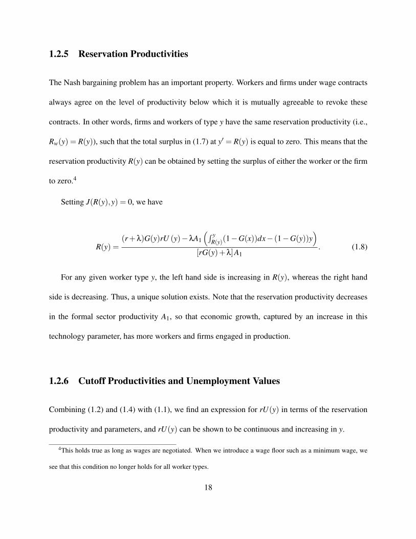
1.2.5 Reservation Productivities

The Nash bargaining problem has an important property. Workers and firms under wage contracts

always agree on the level of productivity below which it is mutually agreeable to revoke these

contracts. In other words, firms and workers of type y have the same reservation productivity (i.e.,

Rw(y) = R(y)), such that the total surplus in (1.7) at y′ = R(y) is equal to zero. This means that the

reservation productivity R(y) can be obtained by setting the surplus of either the worker or the firm

to zero.4

Setting J(R(y),y) = 0, we have

R(y) =(r+λ)G(y)rU (y)−λA1

(∫ yR(y)(1−G(x))dx− (1−G(y))y

)[rG(y)+λ]A1

. (1.8)

For any given worker type y, the left hand side is increasing in R(y), whereas the right hand

side is decreasing. Thus, a unique solution exists. Note that the reservation productivity decreases

in the formal sector productivity A1, so that economic growth, captured by an increase in this

technology parameter, has more workers and firms engaged in production.

1.2.6 Cutoff Productivities and Unemployment Values

Combining (1.2) and (1.4) with (1.1), we find an expression for rU(y) in terms of the reservation

productivity and parameters, and rU(y) can be shown to be continuous and increasing in y.

4This holds true as long as wages are negotiated. When we introduce a wage floor such as a minimum wage, we

see that this condition no longer holds for all worker types.

18

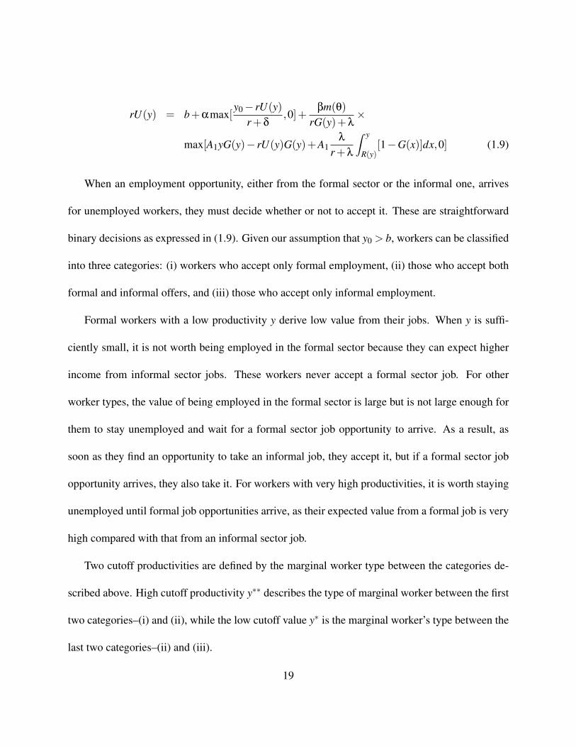
rU(y) = b+αmax[y0− rU(y)

r+δ,0]+

βm(θ)

rG(y)+λ×

max[A1yG(y)− rU(y)G(y)+A1λ

r+λ

∫ y

R(y)[1−G(x)]dx,0] (1.9)

When an employment opportunity, either from the formal sector or the informal one, arrives

for unemployed workers, they must decide whether or not to accept it. These are straightforward

binary decisions as expressed in (1.9). Given our assumption that y0 > b, workers can be classified

into three categories: (i) workers who accept only formal employment, (ii) those who accept both

formal and informal offers, and (iii) those who accept only informal employment.

Formal workers with a low productivity y derive low value from their jobs. When y is suffi-

ciently small, it is not worth being employed in the formal sector because they can expect higher

income from informal sector jobs. These workers never accept a formal sector job. For other

worker types, the value of being employed in the formal sector is large but is not large enough for

them to stay unemployed and wait for a formal sector job opportunity to arrive. As a result, as

soon as they find an opportunity to take an informal job, they accept it, but if a formal sector job

opportunity arrives, they also take it. For workers with very high productivities, it is worth staying

unemployed until formal job opportunities arrive, as their expected value from a formal job is very

high compared with that from an informal sector job.

Two cutoff productivities are defined by the marginal worker type between the categories de-

scribed above. High cutoff productivity y∗∗ describes the type of marginal worker between the first

two categories–(i) and (ii), while the low cutoff value y∗ is the marginal worker’s type between the

last two categories–(ii) and (iii).

19

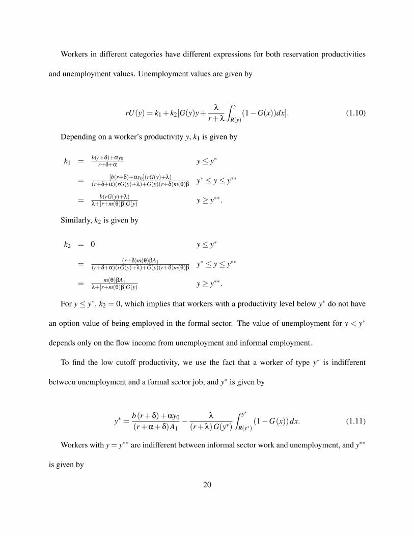
Workers in different categories have different expressions for both reservation productivities

and unemployment values. Unemployment values are given by

rU(y) = k1 + k2[G(y)y+λ

r+λ

∫ y

R(y)(1−G(x))dx]. (1.10)

Depending on a worker’s productivity y, k1 is given by

k1 = b(r+δ)+αy0r+δ+α

y≤ y∗

= [b(r+δ)+αy0](rG(y)+λ)(r+δ+α)(rG(y)+λ)+G(y)(r+δ)m(θ)β y∗ ≤ y≤ y∗∗

= b(rG(y)+λ)λ+[r+m(θ)β]G(y) y≥ y∗∗.

Similarly, k2 is given by

k2 = 0 y≤ y∗

= (r+δ)m(θ)βA1(r+δ+α)(rG(y)+λ)+G(y)(r+δ)m(θ)β y∗ ≤ y≤ y∗∗

= m(θ)βA1λ+[r+m(θ)β]G(y) y≥ y∗∗.

For y ≤ y∗, k2 = 0, which implies that workers with a productivity level below y∗ do not have

an option value of being employed in the formal sector. The value of unemployment for y < y∗

depends only on the flow income from unemployment and informal employment.

To find the low cutoff productivity, we use the fact that a worker of type y∗ is indifferent

between unemployment and a formal sector job, and y∗ is given by

y∗ =b(r+δ)+αy0

(r+α+δ)A1− λ

(r+λ)G(y∗)

∫ y∗

R(y∗)(1−G(x))dx. (1.11)

Workers with y = y∗∗ are indifferent between informal sector work and unemployment, and y∗∗

is given by

20

y∗∗ =(rG(y∗∗)+λ)

βm(θ)G(y∗∗)A1(y0−b)+

y0

A1− λ

(r+λ)G(y∗∗)

∫ y∗∗

R(y∗∗)[1−G(x)]dx. (1.12)

1.2.7 Steady-State Conditions in Urban Areas

The model’s steady-state conditions allow us to solve for the distribution of workers of type y be-

tween sectors. Let u(y), n0(y), and n1(y) be the fractions of workers of type y in unemployment,

informal sector employment, and formal sector employment, respectively, with u(y) + n0(y) +

n1(y) = 1. We implicitly assume for now that the fractions of workers of type y in agricultural

employment is zero whenever u(y)+n0(y)+n1(y) = 1. This implicit assumption will be straight-

forward after no-migration conditions are explained in the following sections.

Workers of type y < y∗ flow back and forth only between unemployment and employment in

the informal sector. The steady-state condition for these workers is given by

αu(y) = δ(1−u(y)).

We then have

u(y) =δ

δ+α

n0(y) =α

δ+α(1.13)

n1(y) = 0.

There are two steady-state conditions for workers with y∗ ≤ y ≤ y∗∗; (i) the flow between un-

employment and informal sector employment and (ii) the flow between unemployment and formal

21

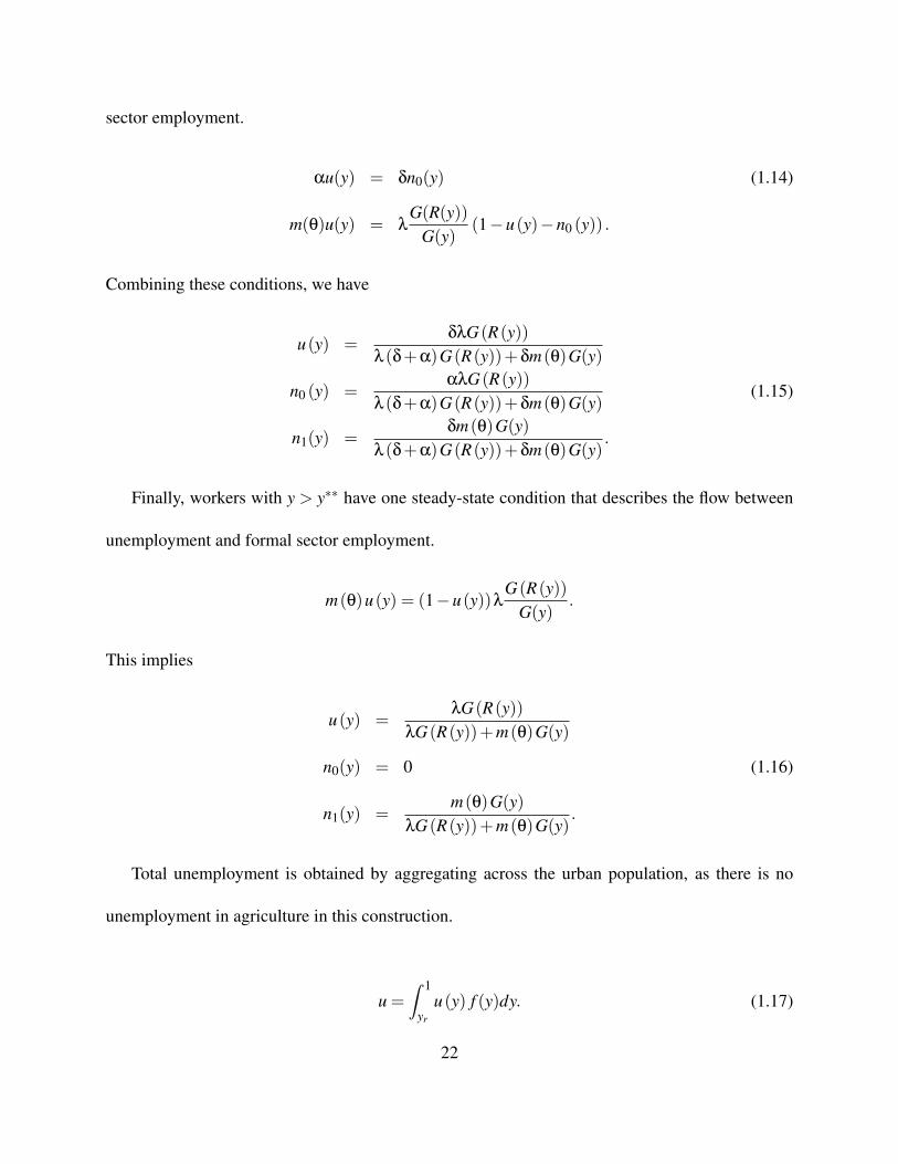
sector employment.

αu(y) = δn0(y) (1.14)

m(θ)u(y) = λG(R(y))

G(y)(1−u(y)−n0 (y)) .

Combining these conditions, we have

u(y) =δλG(R(y))

λ(δ+α)G(R(y))+δm(θ)G(y)

n0 (y) =αλG(R(y))

λ(δ+α)G(R(y))+δm(θ)G(y)(1.15)

n1(y) =δm(θ)G(y)

λ(δ+α)G(R(y))+δm(θ)G(y).

Finally, workers with y > y∗∗ have one steady-state condition that describes the flow between

unemployment and formal sector employment.

m(θ)u(y) = (1−u(y))λG(R(y))

G(y).

This implies

u(y) =λG(R(y))

λG(R(y))+m(θ)G(y)

n0(y) = 0 (1.16)

n1(y) =m(θ)G(y)

λG(R(y))+m(θ)G(y).

Total unemployment is obtained by aggregating across the urban population, as there is no

unemployment in agriculture in this construction.

u =∫ 1

yr

u(y) f (y)dy. (1.17)

22

Analogously, we can compute the total share of workers in the informal and formal sectors.

The share of workers in the formal sector is given by

n1 =∫ 1

yr

n1 (y) f (y)dy,

and the share of workers in the informal sector is

n0 =∫ 1

yr

n0 (y) f (y)dy.

By this construction, n0 +n1 +u+F(yr) = 1.

1.2.8 No-Migration Condition(s)

We assume that if workers migrate to urban areas, they start off unemployed and that workers in the

urban sectors consider migrating back to rural areas only when they find themselves unemployed.

If urban workers migrate to rural areas, they can start working as agricultural workers immediately.

Thus, agricultural work is always available. This means that the migration decision is essentially

one of comparing the value of being unemployed U(yr) with that of being in the agricultural sector

Na(yr) and the migration cost M. In equilibrium, no migration takes places, which means that for

all workers located in rural areas,

rNa(yr)≥ rU(yr;θ)−M (1.18)

and for all workers located in the urban areas

rU(yr;θ)≥ rNa(yr)−M. (1.19)

23

Unilateral (Rural-to-Urban) Migration

With numerical simulations in mind, we think of the benchmark as the state before recessionary

economic shocks. Thus, urban sectors typically attract workers from rural areas in the process of

economic development. Then, the no-migration condition requires

rNa(yr) = rU(yr;θ)−M, (1.20)

and the share of workers in agriculture is la = F(yr), which, combined with the fact that rNa(yr) =

Aalγ−1a , implies

Aa [F(yr)]γ−1 = rU(yr;θ)−M (1.21)

Depending on parameter values, specifically on whether yr is greater or less than y∗, U(yr)

may or may not depend on yr and θ. If yr < y∗, then U(yr) is a constant equal to b(r+δ)+αy0r+δ+α

for all

y ∈ [yr,y∗], but if yr ≥ y∗, then U(yr) is increasing in both yr and in θ. In this latter case, equation

(1.21) defines a locus of (yr,θ) combinations that are consistent with the no-migration condition.

If y > y∗∗, there would be no informal sector, and we exclude this possibility from our analysis.

Figures 2 and 3 illustrate both cases.

The Job Creation Condition

We use the free-entry condition to close the model and determine equilibrium labor market tight-

ness. Setting V = 0 gives

c =m(θ)

θE max[J(y,y),0].

24

To determine the expected value of meeting a worker, we need to account for the fact that the

density of types among unemployed workers is contaminated. Let fu(y) denote the density of types

among the unemployed. Using Bayes’ Law, we have

fu(y) =u(y) f (y)

u.

The free-entry condition can thus be rewritten as

c =m(θ)

θ

∫ 1

max[yr,y∗]J(y,y)

u(y)u

f (y)dy.

This expression takes into account that no jobs will be created for y < y∗, so that the lower limit

of integration is the highest between yr and y∗. If yr < y∗ , then the lowest level of skills for which

it is worth engaging in production is y∗. If yr > y∗ , then the lowest worker type in the urban sector

is yr. After substitution for J(y′,y) evaluated at y′ = y, this becomes

c =m(θ)

θ

(1−β)A1

r+λ

∫ 1

max[yr,y∗][y−R(y)]

u(y)u

f (y)dy. (1.22)

Equation (1.22) is equivalent to the job creation condition in Mortensen and Pissarides (1993),

and it is an equation of θ, R(y) and yr. It only makes sense if the right-hand side is positive. Because

J(y∗,y∗) = 0 and J(y,y) is increasing in y for y ≥ y∗, a necessary condition for equation (1.22) to

have a solution is maxy∗,yr< 1.

Equilibrium with Rural-to-Urban Migration Only

The job creation condition and the no-migration condition jointly determine the equilibrium levels

of θ and yr. There are two cases depending on whether y∗ > yr or y∗ < yr. Figure 4 and 5 illustrate

25

each case. Our equilibrium concept is more general than the one in ANV (2009) in that they only

consider the case y∗ > yr. Thus, they think that there always exist sufficiently low-skilled workers,

who are engaged only in the informal sector. By incorporating the case y∗ < yr, we include urban

labor markets where all unemployed urban workers are potential candidates for formal sector jobs.

All the other components of equilibrium are the same as in ANV (2009).

1.2.9 Bilateral Migration

As observed in Thailand and Indonesia during the Asian financial crisis, return migration may

occur in the labor market adjustment process against economic shocks. Thus, we need to specify

no-migration conditions in which workers are allowed to migrate in both directions. Although eco-

nomic shocks can relocate workers across sectors, not all shocks generate migration. Movements

between urban and rural areas may take place only when the gain from migration is big enough to

cover the migration cost.

Thus, equilibrium in this case requires that for all workers located in the rural areas,

rNa(yr;ypr )≥ rU(yr;yp

r ,θ)−M (1.23)

and for all worker types located in the urban areas,

rU(yr;ypr ,θ)≥ rNa(yr;yp

r )−M. (1.24)

Notice that the no-migration condition is characterized as conditional on the threshold value ypr .

This ypr is needed to pin down yr, and we may consider yp

r as the threshold value of the no-migration

26

condition(s) before an economic shock.

Let ya be the value of y for which equation (1.23) holds with equality

rNa(ya) = rU(ya)−M (1.25)

and let yc be the value of y for which for which equation (1.24) holds with equality

rNa(yc) = rU(yc)+M (1.26)

Figure 6 illustrates the above equations for the case where ya < y∗.

Two things are worth noting. For any equilibrium, i) yc < ya, and ii) there are no workers with

y < yc located in the urban areas and with y > ya located in rural areas. However, workers with

yc < y < ya may be located in either rural or urban areas and still behave optimally in their choice

of location.

Once a shock hits the economy, yr is necessarily yc ≤ yr ≤ ya in a new equilibrium, and this

level of skills may imply some migration if yr 6= ypr . No migration occurs if yc ≤ yp

r ≤ ya because

rNa(ypr ;yp

r )≥ rU(ypr ;yp

r ,θ)−M and rU(ypr ;yp

r ,θ)≥ rNa(ypr ;yp

r )−M. In this case, yr = ypr , and the

case is illustrated by a point like B in figure 6, where B represents the initial threshold level of

skills ypr . If, on the other hand, yp

r < yc, then it is optimal for some workers in the urban sector

to move back to agriculture5 and yr = yc. This case is illustrated by a point like A in the figure.

Finally, if ypr > ya, then it is optimal for some agricultural workers to migrate to the urban areas6

5In this case, rU(ypr ;yp

r ,θ)< rNa(ypr ;yp

r )−M. Thus, some urban unemployed workers can be better off when they

migrate into agriculture.6In this case, rNa(y

pr ;yp

r )< rU(ypr ;yp

r ,θ)−M

27

and yr = ya.

Thus, for an initial allocation of workers determined by ypr , the equilibrium threshold level of

skill is given by:

yr =

yc, yp

r < yc < yat

ypr , yc < yp

r < ya

ya, yc < ya < ypr

(1.27)

Equilibrium with Bilateral Migration

A steady-state multi-sector labor search and matching equilibrium is characterized by a labor mar-

ket tightness θ and no-migration cutoff value yr together with a reservation productivity function

R(y), unemployment rates u(y), and cutoff values y∗, y∗∗, ya and yc and a given latest no-migration

cutoff value ypr such that

(1) the value of maintaining a vacancy is zero.

(2) matches are consummated or dissolved if and only if it is mutually profitable to do so.

(3) the steady state conditions hold.

(4) formal sector matches are not worthwhile for workers with y < y∗.

(5) informal sector matches are not worthwhile for workers with y > y∗∗.

(6) Given ypr , the no-migration condition holds and is determined by (1.23)-(1.27).

28

1.3 Simulating the Impact of Economic Shocks

Economic shock can affect either entire economy or selected firms. For example, a financial shock

can affect entire economy because generally, tightened credit markets make it more expensive to

finance firms production schedules due to increase in the rental price of capital. However, the

shock can negatively affect mainly exporting firms if the shock is originated in foreign importing

countries and domestic economy is relatively immune to the shock. Another example may be food

price shock that we observed in 2007-2008, and natural catastrophes like Haiti’s earthquake in 2010

and Tsunami triggered by Indian ocean earthquake of Sumatra in 2004. In all cases, wages and

employment are adjusted to the shocks, and our purpose of simulation exercises is to quantitatively

evaluate how wages and labor composition are changed when economic shock hits the economy.

If the shock affects entire economy, we view the shock as a structural perturbation on A1, y0,

and/or A0 in our model. That is, as TFP in the formal, informal and/or agricultural sector falls,

all firms are either directly or indirectly affected. The economic shock can affect some firms but

not all of them. In this case, job turbulence in the economy increases, which can be interpreted as

an increase in the arrival rates of idiosyncratic shocks (λ and/or δ) to the formal and/or informal

sector in our model.

Do the impacts of increased turbulence or reduced profitability in the formal sector trickle down

to the informal sector or even to the agricultural one? Although impacts on the other sectors are

quite complicated to estimate empirically, post-crisis labor statistics in developing countries show

significant changes in the informal sector (i.e., an increase in informal employment share, reduced

employment duration, etc.). Because we aim to measure direct and indirect trickle-down effects of

29

the economic shock in labor markets, we evaluate the effect by simulation in our model.

1.3.1 Data

We use several data sources to construct target statistics for our calibration. The main source

is from Nicaragua’s 2001 annual Household Survey (Encuesta de medicion del Nivel de Vida

(EMNV)), in which we find the share of workers in each sector and their level of income and

education. We also use data from the Food and Agriculture Organization (FAOSTAT) to calibrate

the agricultural production function.

Before we discuss the parameterization and calibration strategy of our model, we need to define

which employed worker types are classified into each sector and how broad a concept of unem-

ployment we should employ. We assign family enterprise workers and individually self-employed

and non-regulated wage workers7 outside of agriculture to the informal sector. Regulated wage

workers are assigned to the formal sector, and agricultural workers other than employers are all as-

signed to the agricultural sector. Employers in both agriculture and non-agriculture sectors are left

out all together. We think that they are better understood as firms rather than as workers. Overall,

informality is distinguished from formality in terms of the degree of labor productivity, on the one

hand, and the compliance with labor regulations, on the other.

The transition rate from non-employment to employment is similar among the discouraged,

temporarily inactive and (narrowly defined) unemployed, and so is the rate of transition in the

opposite direction. This suggests that those unemployed workers may not be that different from

7Non-regulated wage workers are those who are not subject to social security payment, while the regulated wage

workers are the opposite.

30

the discouraged and temporarily inactive ones in terms of the willingness to work. We thus use a

broad concept of unemployment that encompasses discouraged and temporarily inactive workers.8

While the narrow unemployment rate is around 4%, the broad unemployment rate is 12%. Table 1

shows the share of workers in each labor market state.

1.3.2 Parameterization

We opt for normalizing some of the parameters to reduce computational burdens. The leisure value

of unemployment is normalized to zero, or the parameter b is fixed at zero; the bargaining power

of formal sector workers is set at the standard value 1/2, or β is equal to 1/2; r, the discount rate,

is set at 0.04.

We first specify parameters of the shock process G(y′) and the skill distribution F(y). We

assume that the idiosyncratic shock process is characterized by a uniform distribution with support

of [0,y]. In other words, when a shock arrives, the new level of productivity of a worker type y lies

between 0 and y, with equal probability of ending up anywhere in the support.

We assume that the skill distribution follows the β-distribution. There are two reasons for this

choice. First, the β-distribution is defined on a finite support so that we can control for extreme

values of skill, and second, the β-distribution is flexible in that it displays a broad range of shapes

depending on the values of two distributional parameters (aβ,bβ). We proxy the skill by the nor-

malized values of education9, and the first two moments of the values of education are sufficient

to calculate the two distributional parameters and thereby, to define the distribution itself.

8See Appendix A for the logic in greater detail9The level of education is normalized by the maximum level in the data.

31

Earnings in agriculture are given by the average product of labor, which is rewritten below:

ya = Aalγ−1a . (1.28)

We estimate the elasticity of agricultural labor (γ) from longitudinal data on agricultural pro-

ductivity and employment from 1961 to 2005.10 We construct the series of the working age popu-

lation in the agricultural sector from the FAOSTAT. We estimate the following simple model,

logYa = c+ γ logLa,

and our estimate of γ is 0.628.

Using the fact that the income from agriculture is given by (1.28), we back out Aa in a way that

is consistent with our data for year 2001. The household survey EMNV enables us to calculate the

average labor income in agriculture (ya) and the share of the workers in agriculture la. The average

income in agriculture is C$10,717 cordobas, and la is 27.10% as shown in Table 1. This allows us

to back up Aa. Finally, when we know γ, Aa, and the average agricultural income, la = 27.1% in

Table 1, this implies that yr is determined at la = F(yr).

The informal labor market is specified by the three parameters α,y0,δ. The average income

in the informal sector (y0) is estimated from the EMNV and is y0 = C$9,767 cordobas. Because

the rate of the informal job destruction (δ) is assumed to follow the Poisson distribution, the inverse

of the rate (i.e., 1/δ) is equivalent to the average duration of holding an informal sector job. Since

we can calculate the duration of informal sector jobs from the EMNV, we can back out δ.

10We use the longitudinal series of the agricultural output Ya published by the Central Bank of Nicaragua.

32

We still have five more parameters to determine.11 As far as we know, we do not have relevant

data available to fix these parameters. We thus calibrate our model to choose the values of the

parameters in such a way as to best match the following target statistics.

We choose the share of workers in formal and informal sector jobs (N0 and N1 respectively), the

average wage w in the formal sector, and the average duration of formal sector jobs d1, for which

our model gives explicit expressions12, and we choose values observed in the EMNV. These targets

are chosen because our model can describe labor markets along those dimensions; examples are

labor market composition, sectoral employment duration and sectoral labor income distribution.

The target statistics from the EMNV are listed in Table 2.

Because the model is able to generate those targets without knowing the migration cost M

and the cost of vacancy c, we first calibrate the model without the job creation and no-migration

conditions to find the values of α,λ,A1, and m(θ). Once these parameters are determined within the

model, the free-entry condition together with the matching specification determines the parameter

c, while M is determined by the no-migration conditions.

1.3.3 Results

Table 3 shows the resulting parameter values, and Table 4 shows the values of endogenous vari-

ables. There is a huge wage difference (w vs ya) between the urban formal and the rural agricultural

11The list is as follows: the arrival rate of the informal employment opportunities (α); the arrival rate of the idiosyn-

cratic shock (λ) in the formal jobs; the formal sector productivity (A1); the migration cost M; and the cost of posting a

vacancy c.12See Appendix B.

33

workers, as there is a difference in the level of technology between the rural agriculture sector (Aa)

and the urban formal sector (A1). As a result, the sector in which one works can be an important

indicator of one’s earning capacity (or individual skill in our model). Given the idiosyncratic shock

arrival rate λ = 0.2342, formal sector jobs are expected to face a shock every four years. Some

might be destroyed and others not, depending on the value of a new productivity draw. However,

we are not able to observe this level, due to the lack of related information from industrial statistics.

The rate of shock arrival to informal sector jobs is around half of the value of λ. This does not

mean that informal jobs are more secure, as they are destroyed whenever a shock arrives. In fact,

formal sector jobs are more stable in the sense that the duration of formal sector employment is,

on average, longer than the duration of informal sector employment by three and half years, which

is directly verifiable from the duration data we used to construct duration targets.

Workers with more than 8 years of education search for jobs only in the formal sector, and

their share of total formal sector employment is about 57% . According to the EMNV, the average

education of formal sector workers is around 8 years, and about 42% of formal sector workers have

more than 8 years of schooling. Our benchmark value of y∗ suggests that workers with less than

complete primary education (6 years) will not search for formal employment opportunities. The

data suggests that only about 30% of informal sector workers have more than 6 years of education.

The no-migration condition suggests that 3 years of education represent the minimum level

required to migrate into urban areas. About 55% of workers in agriculture have less than 3 years

of education.13 Segmentation by skill thus seems to be a clear feature in the Nicaraguan data.

13The percentage of workers with less than 3 years of education falls to 27% in the informal sector and 13% in the

formal sector.

34

1.4 Simulation Results

We simulate the effects of i) 5% and 10% reductions in both the formal sector and the informal

sector TFPs respectively, a 10% reduction in A1 and 5% increase in y0, ii) 5% and 10% increases

in formal sector job turbulence λ respectively, iii) an increase in informal job turbulence δ, and iv)

several combinations of the above.14 The results are listed in Table 5 and Table 6.

Several results are worth highlighting. First, as shown in Table 5, the fall in the formal sector

productivity A1 (Simulation 1) reduces the formal employment regardless of the direction of the

changes in y0. If the shock we consider mainly affects firms in the formal sector (especially,

exporting firms), the impact to informal sector firms should be made through indirect channels, and

the magnitude of negative impact should be smaller than or equal to the change in A1. Thus, the

first two results in Simulation 1 suggest that with the same percentage decline in the productivity

of both sectors or with the urban sectoral productivity shock, the impact is severe in the formal

sector, and some of formal sector workers are relocated to the informal sector.

The third exercise in Simulation 1 describes a case where the productivity in the informal sector

increases. This case may be justifiable because labor productivity in the informal sector can go

up when some relatively productive formal sector workers may be relocated to the informal sector

from the negative TFP shocks in the formal sector. The third result in Simulation 1 suggests that the

magnitude of labor relocation from the formal sector becomes larger as the value of informal sector

jobs increases, in contrast with the other two cases in Simulation 1. Simultaneously, we observe

14In other words, we view the financial shocks as if they are equivalent to decreases in formal sector productivity,

either an increase or decrease in informal sector productivity, an increase in job turbulence or some combinations of

these.

35

from Table 6 that per capita output15 falls, ranging from 3% to 9% in Simulation 1. Therefore, a

1% decline in total output would be associated with a reduction in formal jobs of approximately

0.3% in the first two cases and 6% in the third one.

Formal sector employment is relatively sensitive to changes in A1 and y0, whereas both total

employment and total output are much less responsive. The reason for this is that many workers,

in the face of negative shock on A1, become indifferent between formal and informal sector jobs,

so that workers who searched only for formal sector jobs before the shock are willing to accept

informal sector jobs in the post-shock state of the economy.16 This is a direct consequence of no

rigidities in wages so that wages can absorb part of the decrease in productivity in the formal sector

on one hand and low income of the unemployed (i.e. b = 0) on the other. Consequently, changes in

unemployment and total output are negligible because more workers are attracted to the informal

sector.

In all cases in Simulation 1, the change in unemployment is modest relative to the labor reloca-

tion from the formal sector to the informal sector. For example, the second result in Simulation 1

suggests that 85% of the relocated workers from the formal sector are reemployed in the informal

sector, whereas only 15% of them are unemployed. The level of labor relocation from the formal

sector critically depends on the directional change of informal sector productivity. If both A1 and

y0 decline, the role of the informal sector as a buffering sector becomes weaker, such that the labor

relocation from the formal to the informal sector is relatively small. The second result in Simu-

lation 1 shows a 1% expansion of the informal sector as a result of 10% productivity decline in

15Per capita output is computed as an average income without including the cost of vacancy.16This change in job search behavior is from relatively large increases in y∗∗ in our model.

36

both sectors. If we reduce the formal sector productivity by 10% while holding y0 at the bench-

mark, the informal sector expands by 4%. Furthermore, the third result in the simulation shows the

expansion of the informal sector more than 10% with 10% reduction in A1 and 5% increase in y0.

The second simulation explores the effects of idiosyncratic individual skill shocks in the formal

sector; that is, we experiment with the impacts of a shock that affects some firms in a sector but

not all of them. The skill shocks measure the degree of turbulence in the formal sector. Since the

idiosyncratic formal shocks affect only some individual workers, overall labor markets are much

less affected. However, it is important to highlight that the calibrated turbulence parameter is rather

small at the benchmark. The rate of the shock is 0.2342, so a 10% increase means that, on average,

a firm faces a shock every 3.8 years rather than every 4 years.

The effect of the higher turbulence is to shed workers from the formal sector into unemploy-

ment. Consequently, unemployment rate increases together with shortened duration of formal

sector jobs, as shown in Simulation 2 in Table 5 and Table 6. In this case, we also observe labor

relocation from the formal to the informal sector because the value of a formal sector job declines.

The third simulation attempts to isolate the effects of the increased informal sector job turbu-

lence δ. Again, the benchmark calibrated value of the shock is rather small.17 What we emphasize

in this simulation is that the turbulence in the informal sector alone can relocate workers across

sectors.

A 10% increase in the informal sector turbulence δ increases the formal sector employment

and total unemployment. Since the value of informal jobs declines, more workers search for for-

17The benchmark value of δ is 0.176. In other words, the shock arrives to workers every 5.6 years on average.

37

mal sector jobs.18 The greater turbulence increases the unemployment rate, as informal jobs are

destroyed more frequently. Finally, its impact on welfare is negative, as per capita output decreases

by slightly less than 1%.

Simulations 4 and 5 allow multiple sources of shocks. The main implication is that the effect of

shocks on the formal sector is overall more severe than that on the informal sector. Consequently,

some formal sector workers are relocated into either informal sector or unemployment. However,

the magnitude of the relocation critically depends on whether the informal sector productivity

increases or decreases in the adjustment process following the shock. Overall, unemployment

rates in all our simulation exercises increase as job turbulence in each sector becomes stronger.

However, quantitatively, the rates increase at best 2% in our simulation exercises, as shown in

Table 5.

The biggest effects on wages are obtained when the productivity in both sectors declines and

the turbulence in both sectors increases. In this case, the employed workers in the formal sector

become less productive and thus earn less from their jobs. This is also the case in the informal

sector. Because the buffering role of the informal sector is weakened in this case, formal sector

workers would rather remain in the same sector and take the reduced wages than switch to informal

sector jobs.

It is important to highlight that our model does not consider congestion externalities by the

increase in the number of workers willing to accept informal jobs. Nor does the model consider

effects of the inflow of workers to the informal sector on informal earnings. If there are congestion

externalities or the larger supply of workers to informal sector reduces earnings, a shock to the

18In our model, both cut-off values y∗,y∗∗ decrease, such that more workers become potential formal sector workers.

38

formal sector might generate a larger relocation of workers to agriculture, as well as more unem-

ployment, as the returns to informal employment will decrease. Thus, the economic shock might

have a larger effect on backward migration.

1.5 Conclusions

This paper presents a multi-sector labor search and matching model for developing countries.

Workers in our model are heterogeneous in terms of their skill and are located in one of the three

job sectors or in unemployment. There is an entry barrier between urban sectors and agriculture,

such that workers must pay a migration cost when they migrate into the urban area from the rural

one. The governing principle behind our model is based on the fact that sectors are segmented by

the level of sectoral productivities from different forms of earnings functions, while heterogeneous

workers are endogenously sorted into these sectors. This sorting mechanism is such that high-

skilled workers tend to be located in the relatively more productive and urban formal sector; on the

other hand, low-skilled workers are found in the agricultural or urban informal sectors. However,

some workers in the urban area are indifferent between formal and informal jobs, due to costly job

search frictions.

We use our model to assess the potential effects of the economic shock. The first challenge is

how to model the economic shocks and then to simulate the impacts of the shocks. For example,

how much should the productivities in the formal and other sectors be changed? Most analyses

reduce the effects of the shocks to a measure of growth lost or reduction of GDP. Although both

measures are good indicators for impacts, they are themselves the results of the shocks to exoge-

39

nous variables such as financial instrument variables, foreign demand, etc. We thus construct the

model to describe the underlying mechanism that links the shocks to its endogenous outcomes (i.e.,

GDP per capita, employment and earnings).

Most studies use a measure of projected GDP growth together with employment elasticity

to forecast the effects on labor markets. The elasticity is a summary variable of how these two

variables have responded in the past to exogenous changes. There are two drawbacks to this

methodology. First, the elasticity masks important labor relocation that is likely to have important

effects on welfare and poverty. Second, elasticity might change due to the new conditions in the

world economy. Our model does not imply constant elasticity, and it highlights the relocation of

the labor and its effects on welfare and earnings.

After constructing the model, we try to ascertain in our simulations the degree to which the

economic shocks would affect firms’ profitability and job turbulence.19 The results suggest that

despite modest changes in total employment, there are either significant labor relocations or formal

sector wage-cuts, depending on whether informal sector productivity increases or not.

In Nicaragua, the adverse productivity shock in the formal sector can reduce formal sector em-

ployment. If the informal economy remains unaffected, it may provide these unemployed workers

with a safety net, and unemployment may not significantly increase. However, if the informal

19Firm profitability is well captured in our model by the parameters A1,A0 and yo, and it should not be hard to find

empirical data to estimate the potential effects of changes in these parameters. Job turbulence may have an empirical

counterpart in phenomena such as export sector shocks, but it is hard to identify the effects of those shocks in the data.

As a result, it would be necessary to have an empirically measurable definition of turbulence and to study the impacts

of it in previous crises to adequately simulate it.

40

sector is also affected, then some workers may go back to agriculture reducing the congestion in

the urban labor market, which in turn reduces the impact on the unemployment rates. Thus, unem-

ployment increases modestly at best. The way that the economic shock affects relative returns to

each sector would determine the sectoral relocation of labor and the associated losses in efficiency.

41

42

Chapter 2

Validating a Multi-sector Labor Search and

Matching Model for Developing Countries

2.1 Introduction

The objective of this paper is to validate the use of a multi-sector labor search and matching model

in order to explain labor market structures in developing countries. Labor markets in developing

countries have distinctive features; in particular, a high-skilled productive sector often coexists

with a low-skilled labor intensive sector and a subsistence agriculture. This motivates us to model

labor markets in developing countries using a segmented labor market framework rather than the

conventional competitive labor market treatment. Specifically, we use a model by Gutierrez, Paci

and Park (2008)1, which is an extension of Albrecht, Navarro and Vroman (2009).

Our model validation will allow us to check whether the model is able to reproduce the structure

1Hereafter, we denote them by GPP.

43

of actual labor markets. Specifically, we test whether the model can predict labor market outcomes

not used for our model calibration. For this validation exercises, we first calibrate our model to

the Indonesian labor market in 1997. We then compare our simulated outcomes to data observa-

tions. We find that the model can replicate average skill distributions across sectors, and that both

sectoral employment and unemployment shares across individual skill levels fit well with the data.

However, the unemployment share for highly educated workers is low in the data, whereas our

model predicts a high unemployment share. Additionally, the model-generated wage distribution

is bell-shaped with a high-density around the mean, but the empirical distribution is left-skewed.

Our contribution through this paper is to evaluate whether the model can potentially be used to

study labor structures in developing countries. Our results show that the model is well equipped to

study average behavior in segmented labor markets.

In the next section, we briefly summarize the model of GPP. In Section 3, we explain the data

and target statistics for our model calibration. Benchmark parameterization will be discussed in

Section 4. Our results for cross-sectional and dynamic validations will be shown in Sections 5 and

6, respectively. In Section 7, we conclude.

2.2 Model

Since we use the same model as in chapter 1, we will only briefly describe the model elements in

this section. Our model is built on the search and matching model of Mortenssen and Pissarides

(1994) and Pissarides (2000) and incorporates a multi-sector labor market. We closely follow

Albrecht et al. (2009) and Satchi and Temple (2009). As discussed in Satchi and Temple (2009),

44

labor markets are segmented by geographic distance between urban and rural areas, and wages

in the urban formal sector are determined by bargaining. We deviate, however, from the idea of

dualism in the labor markets in the sense that urban informal sectors are not necessarily queuing

sectors for employment opportunities in urban formal sectors.2 As discussed in GPP (2008) and

ANV (2009), the urban informal sector is characterized as an optimal choice for urban workers

with relatively low skills.

The agricultural sector is regarded as one big extended family, and workers are assumed to

equally divide agricultural output from their labor. Agricultural workers can migrate to urban

areas for employment opportunities at a cost. When they arrive in the urban areas, they start

off as unemployed. Urban areas feature both formal and informal sectors. The former is highly

productive and offers bargained wages, while the latter is relatively unproductive and pays a fixed

income. Urban labor markets have search frictions in that it takes time for both labor-searching

firms and unemployed workers to find mutually agreeable counterparts.

2.3 Data and Target Statistics

2.3.1 Data Sources: Sarkernas vs. IFLS

We use the Indonesian Family Life Surveys (IFLS) and Sakernas to construct labor market targets

for our benchmark model calibration. The IFLS is a longitudinal socioeconomic survey that covers

13 out of 27 provinces and represents 83% of the total population. The first wave was conducted

in 1993 (IFLS1), and the fourth wave, fielded in 2007 through 2008, is the latest.

2See Maloney (1999, 2004), and Pratap and Quintin (2006)

45

Sakernas is a main Indonesian labor force survey managed by the BPS3 to monitor and com-

pile provincial employment statistics. It has been conducted since 19864, and the survey covers a

nationally representative sample of about 40,000 of the working-age population. However, Saker-

nas’ lack of self-employment income records fails to identify the informal economy of our model.

Thus, we use the information about self-employment incomes from the IFLS. Although IFLS is not

nationally representative, both Sakernas and IFLS show similar changes in wages and employment

rates over the Asian Financial crisis.5

However, these surveys show opposite trends in the unemployment rate. As shown in Table 7,

the unemployment rate in the IFLS declined from 7.6% to 2.02%, whereas the rate had gone up

from 4.70% to 6.30% in Sakernas through the crisis. As discussed in Smith et al. (2002), this

discrepancy may be due to survey design. Both surveys asked a similar lead-in question. When

respondents answered ’currently not working6’, the Sakernas stops probing further, whereas the

IFLS asks two-step follow-up questions. First, respondents are asked if they had worked for pay

for at least one hour. If they answer ’No’, then the second follow-up question probes whether

they had worked in a family-owned business. Therefore, the IFLS is expected to have a lower

unemployment rate.

The unemployment trend in Sakernas follows the conventional wisdom that labor demand tight-

3It is an abbreviation for Badan Pusat Statistik or Statistics Indonesia. This is a government agency tasked with

collecting and publishing statistical data in Indonesia.4The survey was done quarterly before the year 1995 and annually afterwards.5See Smith et al. (2002)6Work is defined as an employed state in which one generates income or helps to generate income for at least one

continuous hour.

46

ens when the economy is in a downturn. Consequently, more unemployed workers queue, and

queue for a longer time, for employment opportunities in a recessionary state. However, we have

no reasons to reject the fall in unemployment observed in the IFLS. A small decline in unem-

ployment rate may be understood as the informal sector is expanding in economic recession in

developing countries. That is, the observed increase in unpaid family business workers and in fe-

male labor force participation, particularly in the informal sector, may support the low post-crisis

unemployment rate reported by IFLS.

For our target statistics, we use wage and employment statistics from the IFLS and the unem-

ployment rate from the Sakernas.7 For consistency purposes, we restrict samples from the Sakernas

to 17 provinces of the IFLS. As shown in Table 7, the effect of sample selection on unemployment

rates is negligible.8

2.3.2 Labor Composition and Labor Income

In Table 8, we list sectoral employment shares and the unemployment rate in the benchmark In-

donesian labor market. First, we exclude employers to be consistent with the concept of workers in

our model. Employers may be more like firms than workers. We also drop the self-employed with

workers, which consists of 3.6% of the total sample. This variable is characterized in the survey at

2000 by dividing it into self-employed with family member and employer with permanent workers.

We consider the former as self-employed informal workers and the latter as employers. The share

of self-employed with workers takes only 3.6% in 1997, and self-employed with family member as

7The reason why we use Sakernas’ unemployment rate is simply that Sakernas is nationally representative.8The rates in 1997 are the same while there is only 0.2% difference in year 2000.

47

in 2000 might have been absorbed in self-employed working alone, or unpaid family workers in

1997. Thus, we think that the informal sector captures the same characteristics of workers in both

years.9

As discussed in GPP (2008), sample observations are classified into model variables as follows.

All types of workers in the agricultural sector are assigned to agricultural employment. Informal

workers are defined by self-employed working alone, self-employed with family member, unpaid

family workers, or wage workers with no medical or social security contribution. Workers are

employed in the formal sector if they are either government workers or wage/salary workers with

social security.

Table 9 shows labor incomes across sectors. As is the general case in developing countries, an

average formal sector income is highest, and agricultural income is the lowest in Indonesia.

2.4 Benchmark Parameterization

Since we use the same model as discussed in GPP (2008), we closely follow their parameterization

strategy. In this section, we briefly explain our benchmark calibration strategies.10 Our benchmark

calibration is run for the Indonesian labor markets in 1997.

First, we take a discount rate of 0.1381 from the IMF data set. Workers are heterogeneous

and are indexed by their skills. We assume that the skills follow a β-distribution with the support

of [0,1]. This distribution is estimated by taking the level of education as a proxy. Three sectors

are distinguished by sector specific productivities.; Aa for Agriculture, A1 for the formal sector

9In other words, if there is any discrepancy that the informal sector captures, in both years, it should be negligible.10Refer to Appendix B in GPP (2008) for calibration methods in detail.

48

and unity for the informal sector as a normalization. When we rewrite the agricultural production

function, we have

YA = AaNγ

0

We estimate YA and N0 from the IFLS. We fix the agricultural labor elasticity parameter γ at the

poor-country average as in Bravo-Ortega et al. (2004). We then determine the value of Aa within

the model in such a way to match the average income in agriculture.

The model implies that workers sort themselves into sectors such that highly productive work-

ers are more likely to be found in formal sector jobs; low productivity workers in agriculture;

workers in-between are either working in the formal or informal sector, depending on their search

draws. Formally, workers’ choice rules can be characterized by the following cut-off values yr,y∗

and y∗∗. Agricultural workers are the ones whose skills are y < yr. Workers with y∈ [yr,y∗] choose

to work only in the informal sector. If workers’ skills are greater than or equal to y∗, they can

work in either the formal or the informal sector, but workers with y ≥ y∗∗ choose to work only

in the formal sector or to remain unemployed until they find a formal sector job. We determine

yr to match the agricultural worker share. Two cut-off parameters, y∗ and y∗∗, are endogenously

determined in a way to best match our calibration targets.

We have four parameters α,δ,λ,m(θ) that represent frictional urban labor markets. We fix

the parameter for the informal sector job destruction rate (δ) at the value in GPP (2008) to reduce

the computational burden. In this case, we assume that the informal job destruction shocks come

every 5 years on average. Since there are no empirical findings on the shape of the matching func-

tion for developing countries, we assume a standard CRS function from the labor search literature

49

for developed countries. The function is given by

m(θ) = ζθρ.

We take m(θ) as a parameter, set ζ to be unity and use a standard value 1/2 for ρ. The bench-

mark steady-state value of θ is given by θ = m(θ)2.

As discussed in GPP (2008), the migration cost M is given by a no-migration condition, and

the cost of a vacancy C by the formal sector firm’s free-entry condition.

A subset of model parameters α,λ,A1,m(θ) is determined within the model in a way to best

match the employment shares, average formal sector wage11, and unemployment duration. In this

calibration exercise, we have a system of non-linear equations to solve for the unknown parameters.

Generally, it is difficult or impossible to analytically prove both existence and uniqueness of the

solution. Our computational approach is to construct the loss function12 and choose the parameters

that minimize the loss value.

In cases in which uniqueness is guaranteed, the minimization problem above finds the unique

solution. If multiple solutions exist, then we must have a criterion to choose one of them. Since

we use a simplex-based algorithm for the minimization problem, multiple solutions implies that

the solution is not independent of the set of initial guessing values. Thus, our rule to choose the

solution is to create grid lines of parameters for initial guessing values for the candidate solution.

Some initial guessing values end up with non-convergence, and some others may converge. Our

11Average labor incomes in both the agriculture and the informal sector are estimated from the IFLS.12In our case our loss function is the average of the square of the log difference between the data targets and

corresponding model outcomes. The reason why we choose the log difference is that some targets have different units

of measure.

50

choice rule is to have the best solution, or solution of the minimum loss value within the parameter

space we imposed.13

2.4.1 Implications of Benchmark Parameterization

Benchmark parameters are listed in Table 10, and outcome variables are in Table 11. Notice that

our calibration results are quite accurate in the sense that they are matching the targets almost

perfectly.

Differences in sectoral productivities are translated into those in sectoral average incomes.

The results suggest that the formal sector TFP is substantially higher than that in agriculture (e.g.

A1/Aa = 8.7302) while the ratio of the average incomes is w/Ya = 2.8833. Additionally, informal

sector job opportunities come more frequently than formal sector ones. Unemployed workers find

about 1.5 formal job opportunities during each year, on average (e.g. m(θ) = 1.5281), although

they do not necessarily take them. They also meet 4 informal jobs on average (e.g. α = 4.0163).

As with the rate of informal job arrival, the informal job destruction comes infrequently (e.g.

δ = 0.1757). On the other hand, idiosyncratic productivity shocks on formal jobs arrive once in

every 3 years, on average (e.g. λ = 0.3021). In the steady state, a flow value in the formal sector is

greater than that in the informal sector by 2.4%.

The cost of vacancy, C, is about 30% of an average formal sector wage. The cost of migration

takes about 90% of average income in agriculture. For the other parameters, we use either standard

13We bound α ∈ (0,10), λ ∈ (0,5), A1 ∈ (1,5) and m(θ) ∈ (0,10) in our calibration. Thus, our restrictions are such

that both the formal and informal sector job opportunities arrive on average 10 times at best, and the idiosyncratic

shock hits formal sector jobs on average 5 times. The maximum formal sector TFP is constrained to be 5.

51

values in the literature or normalized ones.

In Figure 7, we draw the reservation productivity for formal sector workers. Since yr < y∗ as

shown in Table 11, the level of skill for formal sector workers must be greater than y∗ = 0.3719.

The reservation productivity is flat between y∗ and y∗∗ and increases with y > y∗∗. For workers

with y ∈ [y∗,y∗∗], they have the similar outside option value of unemployment, so that the slope of

the reservation productivity is flat. For workers with y > y∗∗, the outside option value increases

with y. So does the reservation productivity. There is a kink point at y∗∗ = 0.6015 on right hand

side of which the slope of the graph becomes steeper.

Overall, our benchmark calibration shows, as expected, that the formal sector is the most pro-

ductive and has a relatively high rate of job turbulence. Thus, the formal sector has relatively

higher job flow rates14 than informal sector.

2.5 Outcome Validation

In this section, we validate our model by comparing our calibration outcomes with data observa-

tions of Indonesian labor markets in 1997. Thus, this validation exercise is made to the extent

that the IFLS permits. We use the outcomes from these exercises partially to support the use of

the model in characterizing labor markets in Indonesia and developing countries of the similar

characteristics.

There are several outcomes we can use for this purpose. Specifically, we examine 1) skill

distribution, 2) formal wage distribution, 3) structure of segmentation by skill, and 4) employ-

14The job flow rate in the formal sector is 0.7, whereas the rate in the informal sector is 0.46.

52

ment/unemployment composition by skill.

2.5.1 Skill Distribution

Our parameterization assumes that the skill distribution is continuous and follows a β-distribution

with two parameters estimated by a proxy variable years of education.15 The skill distribution is

not the same as the distribution of education.16 The education variable is a proxy in a sense that

labor market segmentation by skills follows closely on the segmentation by the level of education.

Our result suggests that model distribution is smooth and unimodal, whereas the data distribution is

jagged and multi-modal with the peak at 6 years (complete elementary school), 9 years (complete

middle school), and 12 years (complete high school).

Figure 8 draws the skill distributions from the model and data respectively. The differences in

the shapes come mainly from the continuous skill distribution in the model in contrast with discrete

education data. However, the first two moments of the distributions are identical by construction.

Although the simulated skill distribution does not match well with the empirical skill distribution,

the simulated distribution remain useful for describing average behavior of workers in a multi-

sector labor market.

15We first normalize the proxy variable by the maximum years of schooling and then estimate two parameters of

β-distribution in the support of [0,1].16The level of education may be one component included in measuring one’s skill

53

2.5.2 Wage Distribution

Given the level of skill, a formal sector wage is determined by Nash bargaining, and it can be

expressed by a weighted average of a flow value of a worker-firm match and an outside option

value of the worker’s unemployment.17 Since it is impossible or difficult to derive the analytic

expression for the wage distribution, we numerically construct this distribution. Specifically, we

generate employed workers in the formal sector from their skill distribution, and then we simulate

a history of idiosyncratic skill shocks for each worker. The distribution of the idiosyncratic shocks

is constructed from the Poisson distribution with the annual shock arrival rate of λ. As discussed

in ANV (2009), we assume that the idiosyncratic shocks are independent across individuals and

previous history of shocks.

Figure 9 illustrates the observed and simulated wage distributions. Clearly, the distribution in

the data is more dispersed than the one simulated by model parameters. Additionally, the observed

wage distribution has a long right tail, which is not a feature of the simulated distribution.

As the skill distribution is constructed by individual schooling observations, schooling distri-

bution does not have an appropriate shape to match the higher moments of the wage distribution.

In other words, we need to have some other factors to produce the wage dispersion not captured

by the model. One way to improve this distributional discrepancy may be to use a better proxy for

the skill. For example, we may construct the skill distribution by the partial predicted values from

running Mincerian wage equation. In other words, we choose some of independent variables that

is directly related to one’s skill and use the predicted values from only these variables as the proxy

17See the section 1.3.4 in Chapter 1.

54

for the skill. However, since our objective is not to match the wage distribution itself but only the

average wage, this discrepancy is not likely a serious flaw for our purposes.

2.5.3 Structure of Segmentation by Skill

There are two types of segmentation in labor markets. The first one is made by a geographical

distance between urban and rural sectors. When workers in one location migrate into another, they

must bear a migration cost, which works as one type of entry barriers. In equilibrium, workers in

all locations do not have any incentive to migrate.

Another type of segmentation is made within the urban labor markets. It is not profitable for

formal sector firms to hire sufficiently low skilled workers on one hand. The low skilled workers

have no incentives to have a job in the formal sector when their values of the informal sector jobs

are greater than those of formal sector ones, on the other hand. Therefore, there exist some low-

skilled workers who choose to work in the informal sector even when formal sector opportunities

arrive. Similarly sufficiently highly skilled workers choose only formal sector jobs.18

The segmentation in our model is endogenously made by individual skills, which is the main

modeling idea of ANV (2009) and GPP (2008). Model parameters that represent the segmentation

are yr,y∗,y∗∗, where yr is the threshold value of the skill in urban-rural segmentation; y∗,y∗∗

determines formal-informal segmentation in the urban labor market.19 We list sectoral educational

statistics in Table 12.

Average education levels across sectors can be ranked from agriculture to informal and to

18See section 3.6 in GPP(2008).19See ANV (2009) and GPP (2008) for explanation in detail.

55

formal sector in ascending order, which qualitatively matches our model outcomes in Table 12.

Our model can also reproduce the segmentation by skill observed in the data. Overall, our model

is off by 2 years from the average years of education across sectors. Further, notice the average

skill/education of the unemployed workers in both data and model. The average value is slightly

lower than that of formal sector workers. Thus, our model outcome is in line with the view that

unemployment is a ’luxury’, since those high-skilled unemployed workers tend to work in formal

sector and earn relatively high incomes.

2.5.4 Employed Skill Distribution

Figure 10 illustrates the share of workers in each sector across skill levels. The first plot shows

the agricultural sector. Each circle represents the share of workers employed at a given level of

skill. Roughly, 60% of workers with less than 3 years of education are employed in agriculture,

and the percentage decreases as the level of skill increases. Our benchmark result implies that all

workers with the education less than 5.6 years are employed only in agriculture. Qualitatively,

the employment share distribution in agriculture is well squared with data observations in that

relatively low-skilled workers are more likely to be employed in agriculture.

The employment share in the informal sector has an inverse-U shape in our model with respect

to years of education, and it monotonically decreases after 5.6 years. Similarly, the share has an

inverse-U shape in the data as shown in Figure 10. The formal employment share in our model is

monotonically increasing with the level of skill, and so is the share in the data. Overall, Figure 10

shows that relatively, low-skilled workers are found in the rural agriculture in both the model

56

and the data; in urban sectors, the employment share in the informal (formal) sector decreases

(increases) with the level of skill in both the model and the data.

We illustrate the cumulative distributions of skill across sectors from both the model and the

data in Figure 11. First, the model suggests that most workers in the agricultural sector should

have a level of education lower than 6 years. In the data, 80% of workers in the agriculture have

education lower than 5.6 years. Our benchmark result implies that employed formal sector workers

have the level of education above 5.9 years. This also well squares with the data. The data suggests

that 88% of workers in the formal sector have education above 5.9 years.

The second plot in Figure 11 illustrates the distribution of skills in the informal sector. Our

model shows a more concentrated profile of skills in the informal sector than the data draws. In

particular, the model predicts few workers with education below 5.6 years. However, the data

shows that 31% of workers in the sector have a level of education below this level.

Overall, the level of education is a plausible proxy for the skill distribution in a sense that we

match the first moment of the sectoral distributions in our calibration. However, the education

proxy may not be sufficient if our calibration targets higher moments of the distributions.

2.5.5 Unemployment Rates by Skill

Workers in the rural sector are always employed in subsistence agriculture, which acts as employ-

ment of the last resort. As such, the unemployment rate of those low-skilled agricultural workers

should be low. Unemployment is an urban phenomenon, and it is considered as a ’luxury’ that only

highly skilled workers can afford to, and unemployment is only worthwhile if a good employment

57

opportunity is pending. This implies that unemployment rate should rise with education.

Figure 12 illustrates unemployment rates by the level of skill. The observed unemployment

share by level of education is increasing up to 12 years (which amount to 92% of the workforce).

Unemployment shares for those with education less than 7 years are below 7%. For moderate

skilled workers, unemployment shares are between 7% and 14%. However, for workers with more

than 12 years of education, the unemployment share decreases again, suggesting that the opportu-

nity cost of unemployment for high-skilled workers is very high. The model is not able to replicate

this low-unemployment share of the high-skilled workers. However, this should not be a huge con-

cern since these workers represent less than 7% of total workforce. Notice that the unemployment

share is constant for workers with y > y∗∗. High-skilled workers are more vulnerable to unemploy-

ment as their reservation productivity increases in y for y > y∗∗. However, the difference between

one’s potential productivity/skill y and reservation productivity R(y) becomes wider as y increases

for y > y∗∗, so that workers become less vulnerable to unemployment. In equilibrium, two effects

offset each other, and unemployment share become steady for y > y∗∗.

2.5.6 Summary

The model assumes segmented labor markets: a rural agriculture sector, and informal and formal

urban sectors. These sectors have distinct wage-setting mechanisms and production technologies.

Given these sectors, workers, indexed by skills, endogenously choose their sector of work. When

we use the educational attainments as a proxy for skill, our model closely matches an average skill

distribution across sectors. Also, in our model, high-skilled workers are found in the productive

58

formal sector, whereas low-skilled workers are engaged in production at either agricultural or

informal sector. This segmentation by skill is also verified in the data. Further, the unemployment

shares increase with the skill, which is also observed in the data. However, our model fails to

match low unemployment shares for high-skilled workers.

As for the income distribution across sectors, all workers in the agriculture and informal sec-

tors are assumed to earn average income in the data so that our model matches the data means by

construction. Our model generates a wage distribution in the formal sector. Although the model

matches the average wage, its distribution is clustered around the mean, whereas the data distribu-

tion is left-skewed. Overall, we think that the model is well equipped to explain average behavior

of workers in the multi-sectoral labor markets.

2.6 Conclusion

We take a view of segmented labor markets in developing countries and choose a multi-sector labor

search and matching model of GPP (2008). First, we validate our use of the model by comparing

model outcomes with data observations. We show that skill-sector matching patterns are com-

patible between the model and data observation. In other words, high-skilled/educated workers

tend to work in the formal sector, and relatively low-skilled/educated workers in the informal or

agriculture, in both the model and the data.

In summary, the model turns out to be well equipped to explain labor market structure. Given

this validation of the model, we may push a step further into implementing some policy instru-

ments.

59

60

Chapter 3

Quantitative Study of Cross-Country

Intergenerational Mobility

3.1 Introduction

Empirical studies have measured intergenerational labor income1 mobility2 in the U.S. and in

some other countries. These studies’ results are important because they have strong implications

for understanding individual economic success. One’s standing in the income distribution might

be a result of individual effort (i.e., work habits) or acquired ability (i.e., human capital or I.Q.).

However, if those factors are heavily influenced by family background (i.e., family income, social

class and family reputation), one’s standing is at least partially deterministic and moreover, may

1Hereafter, we simply use ’income’ to denote labor earnings.2Intergenerational elasticity as a measure of mobility ranges from 0.3 to 0.6 in the U.S. depending on the data

source and definition. Solon (1999), D’addio (2007), Bjorklund and Jantti (2009) provide surveys of this literature.

61

be sustained throughout generations.

Thus, it is important to study the sources of social standing and the channels through which

social standing is transmitted intergenerationally.3 In this paper, we modify Solon’s (2004) spec-

ification of Becker and Tomes’s (BT) (1992) model and study the quantitative importance of the

sources of cross-country differences in intergenerational income mobility.

As in BT, we consider two factors; namely, human capital investment and ability endowment.

We define human capital as a factor of the income-generating function. Like the BT model, al-

truistic parents provide their children with many learning opportunities so that children may be

equipped with as high an earnings capacity as possible later in their life. The parental resource

allocation for those opportunities is called the human capital investment, and a child’s earnings

capacity reflects his/her human capital holdings.

Thus, the size of the per-unit returns on human capital investments is quantitatively important

for intergenerational mobility. If the returns are relatively large, income-rich altruistic parents

invest more in their children; therefore, income mobility is relatively low. In other words, one’s

standing in terms of the income distribution tends to persist throughout generations.

We consider learning ability as the second source of intergenerational income mobility. Ability

is often decomposed into cognitive and non-cognitive components. Here, we do not make any

distinction between the two types but rather simply use the term ”learning ability”. Learning ability

is understood as an investment-augmenting technology. When two persons have the same level

3D’addio (2007), Bjorklund and Jantti (2009), Altonji and Dunn (1996), and Corcoran et al.(1992) provide empir-

ical analyses of this question. For theoretical references, see Ben-Porath (1967), Becker and Tomes (1992), Han and

Mulligan (1997), Solon (2004) and Huggett et al.(2006).

62

of human capital investment, but their learning abilities are different, the one who has a greater

learning ability can produce a higher level of human capital. Thus, learning ability augments

human capital investment. In other words, the efficiency level of the human capital investment is

higher for someone with a greater learning ability. We assume that learning ability is exogenously

transmitted and follows an AR(1) process.4

Given these channels of mobility, we calibrate the model for 10 OECD countries and discuss

cross-country implications. Specifically, we study how institutional differences represented by dif-

ferent parameterizations are related to intergenerational mobility. We then analyze the importance

of ability transmission and human capital investment with respect to mobility. Finally, we focus

on the impact of a direct governmental subsidy on human capital investment.

Our results are as follows. Mobility in countries with higher returns on the human capital

investment tends to be more intergenerationally related so that one’s standing in the income dis-

tribution depends more on parental income and therefore on the parental human capital invest-

ment. Second, countries with high variation in learning ability transmission tend to generate high

cross-sectional inequality in terms of income distribution. When we focus on how the degree of

intergenerational ability variation affects mobility, it appears that the magnitude of heterogeneity

is not critical in determining mobility. However, when each child is given relatively equal oppor-

tunities in human capital accumulation or provided with relatively homogeneous human capital

4This specification is generally adopted within the theoretical literature. The empirical literature has shown that

learning ability as measured by cognitive ability is intergenerationally correlated and has a significant impact on market

outcomes. This correlation ranges from 0.42 to 0.72 (Daniels et al., 1997, Bowles et al. 2003). The direct effect of

learning ability on market outcomes is 0.15 (Bowles et al. 2003)

63

investments, intergenerational mobility is shown to improve significantly.

Our main contribution to the literature is to quantitatively study the BT model and compare in-

tergenerational human capital transmission functions across countries. The remainder of the paper

proceeds as follows. In Section 2, we describe the dynasty model of human capital investment. In

Section 3, we discuss our benchmark parameterization. In Section 4, we apply the proposed model

to 10 OECD countries and discuss outcomes that explain cross-country intergenerational mobility

patterns. In Sections 5 and 6, we analyze how learning ability variation and direct governmental

human capital investment subsidies affect intergenerational mobility. We conclude the paper in

Section 7.

3.2 Literature

Solon (1992) and Zimmerman (1992) challenged BT’s empirical claim that intergenerational in-

come mobility in the U.S. is no worse than in European countries. This challenge involved method-

ological issues related to life-time income. When life-time income is proxied by the average or

present discounted income for a short time span, Solon (1992) showed that there is an estimation

bias for mobility. Solon (1992) adopted the error-in-variable method to construct life-time income

and found that the U.S. is no better than European countries in terms of intergenerational mobility.

These authors’ method of measuring intergenerational income elasticity (or correlation) has

been widely adopted in country studies.5 Different sample definitions and time periods make

direct international comparisons difficult. Furthermore, estimation methods differ depending on

5Bjorklund et al.(2009) and Solon(2002) provide surveys of such international comparisons.

64

the availability of data. Thus, studies on international income mobility tend to restrict themselves

to the comparison of the regression coefficients of simple linear regression models.

Bjorklund et al.(2009) and Solon(2002) showed that the coefficient of the standard linear model

is around 0.2 for Nordic countries (Denmark, Sweden, Finland and Norway), whereas the coef-

ficient for France, Italy and the U.S. is around 0.4. Using a similar sample, time period and

methodology, Bjorklund et al. (2000) estimated intergenerational income elasticity for the U.S.

and Sweden and showed that the elasticities differ significantly.

These cross-country studies naturally lead us to question what underlying factors cause such

differences. One potential explanation frequently mentioned in the literature is the heterogeneity

of institutions among countries. In our paper, we take BT’s model of human capital investment

and parameterize it for the heterogeneity of institutions.

Our model also builds on the work of Hassler et al. (2002) and Restuccia et al. (2004). Both

studies showed that educational investment (i.e., public education versus productivity growth in

Hassler et al. (2002) and early childhood education versus college education in Restuccia et al.

(2004)) affect both intergenerational income persistence and cross-sectional income inequality.

These studies utilized dynamic general equilibrium models with acquired ability and parental in-

come heterogeneity. The implication of Hassler et al. (2002) was that productivity differences (i.e.,

TFP), rather than public education, cause European countries to be more equal and less mobile than

the U.S. Restuccia et al. (2004) emphasized the role of early educational investment in intergen-

erational mobility and concluded that college education is mainly responsible for cross-sectional

inequality.

65

3.3 Model

We use a two-period overlapping generations model. There is one child and one parent in each

generation. The parents in each generation are assumed to act altruistically toward their immediate

offspring. Because a child is assumed to act altruistically toward his/her future child, a given parent

is essentially altruistic toward all his/her future descendants. This assumption justifies the dynastic

structure of preference because a parent’s actions toward the immediate child ultimately affect the

utility of all descendants thereafter.

The parent at time j earns income y(h j) from his/her human capital h j. Given disposable

income yd(h j), the parent decides how much the family will consume c j and how much to invest

s j+1 in the child’s human capital accumulation. The learning ability a j+1 of the child at time

j+1 is transmitted partly from the parent’s a j and partly by a random environmental effect ε j+1.

Specifically, we assume that learning ability is an AR(1) process.6

Given the structure of the model described above, our problem is characterized by

U(y1;a1) = maxc j,s j+1∞

j=1

E[∞

∑j=1

βj−1u(c j)]

subject to

c j + s j+1 = ydj

log(a j+1) = ρ log(a j)+ ε j+1, ρ ∈ (0,1)

h j+1 = a j+1sγ

j+1 γ ∈ (0,1)

6We use the specification from Becker and Tomes (1986) and Solon (2004).

66

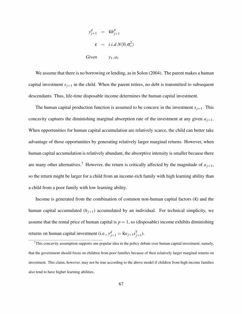
ydj+1 = κhp

j+1

ε ∼ i.i.d.N(0,σ2v)

Given y1,a1

We assume that there is no borrowing or lending, as in Solon (2004). The parent makes a human

capital investment s j+1 in the child. When the parent retires, no debt is transmitted to subsequent

descendants. Thus, life-time disposable income determines the human capital investment.

The human capital production function is assumed to be concave in the investment s j+1. This

concavity captures the diminishing marginal absorption rate of the investment at any given a j+1.

When opportunities for human capital accumulation are relatively scarce, the child can better take

advantage of those opportunities by generating relatively larger marginal returns. However, when

human capital accumulation is relatively abundant, the absorptive intensity is smaller because there

are many other alternatives.7 However, the return is critically affected by the magnitude of a j+1,

so the return might be larger for a child from an income-rich family with high learning ability than

a child from a poor family with low learning ability.

Income is generated from the combination of common non-human capital factors (κ) and the

human capital accumulated (h j+1) accumulated by an individual. For technical simplicity, we

assume that the rental price of human capital is p = 1, so (disposable) income exhibits diminishing

returns on human capital investment (i.e., ydj+1 = κa j+1sγ

j+1).

7This concavity assumption supports one popular idea in the policy debate over human capital investment, namely,

that the government should focus on children from poor families because of their relatively larger marginal returns on

investment. This claim, however, may not be true according to the above model if children from high income families

also tend to have higher learning abilities.

67

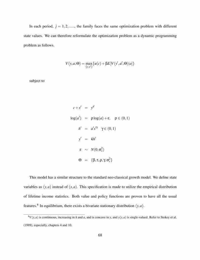
In each period, j = 1,2, ....., the family faces the same optimization problem with different

state values. We can therefore reformulate the optimization problem as a dynamic programming

problem as follows.

V (y,a;Θ) = maxc,s′u(c)+βE[V (y′,a′;Θ)|a]

subject to

c+ s′ = yd

log(a′) = ρ log(a)+ ε, ρ ∈ (0,1)

h′ = a′s′γ γ ∈ (0,1)

y′ = κh′

ε ∼ N(0,σ2v)

Θ = β,τ,ρ,γ,σ2v

This model has a similar structure to the standard neo-classical growth model. We define state

variables as (y,a) instead of (s,a). This specification is made to utilize the empirical distribution

of lifetime income statistics. Both value and policy functions are proven to have all the usual

features.8 In equilibrium, there exists a bivariate stationary distribution (y,a).

8V (y,a) is continuous, increasing in h and a, and is concave in y, and y(y,a) is single-valued. Refer to Stokey et al.

(1989), especially, chapters 4 and 10.

68

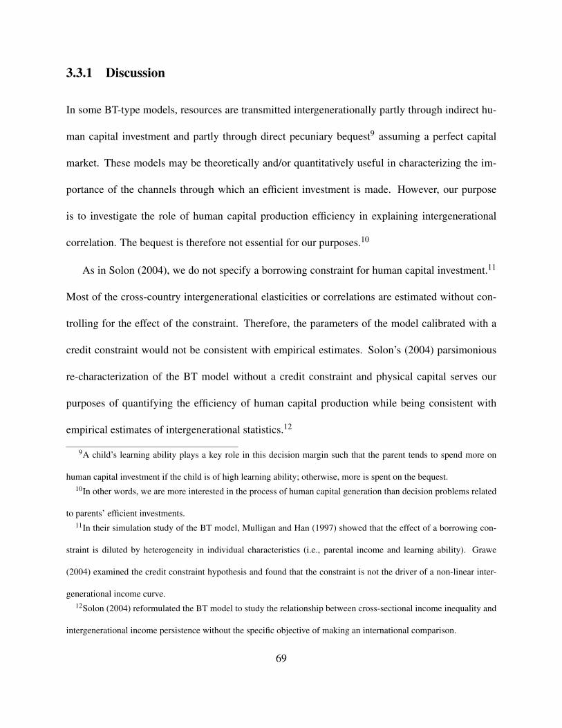
3.3.1 Discussion

In some BT-type models, resources are transmitted intergenerationally partly through indirect hu-

man capital investment and partly through direct pecuniary bequest9 assuming a perfect capital

market. These models may be theoretically and/or quantitatively useful in characterizing the im-

portance of the channels through which an efficient investment is made. However, our purpose

is to investigate the role of human capital production efficiency in explaining intergenerational

correlation. The bequest is therefore not essential for our purposes.10

As in Solon (2004), we do not specify a borrowing constraint for human capital investment.11

Most of the cross-country intergenerational elasticities or correlations are estimated without con-

trolling for the effect of the constraint. Therefore, the parameters of the model calibrated with a

credit constraint would not be consistent with empirical estimates. Solon’s (2004) parsimonious

re-characterization of the BT model without a credit constraint and physical capital serves our

purposes of quantifying the efficiency of human capital production while being consistent with

empirical estimates of intergenerational statistics.12

9A child’s learning ability plays a key role in this decision margin such that the parent tends to spend more on

human capital investment if the child is of high learning ability; otherwise, more is spent on the bequest.10In other words, we are more interested in the process of human capital generation than decision problems related

to parents’ efficient investments.11In their simulation study of the BT model, Mulligan and Han (1997) showed that the effect of a borrowing con-

straint is diluted by heterogeneity in individual characteristics (i.e., parental income and learning ability). Grawe

(2004) examined the credit constraint hypothesis and found that the constraint is not the driver of a non-linear inter-

generational income curve.12Solon (2004) reformulated the BT model to study the relationship between cross-sectional income inequality and

intergenerational income persistence without the specific objective of making an international comparison.

69

We can formulate the human capital generating function as follows.

h j+1 = a j+1(s j+1 + s)γγ ∈ (0,1),

where s is the size of the public human capital subsidy. This specification provides some

dimensions with which to experiment on the influence of a public human capital subsidy on in-

tergenerational mobility. However, it is not clear why both types of investments are additively

specified, especially because the subsidy has the characteristics of a public good. In our model,

this public investment is incorporated multiplicatively and captured by the parameter κ.

3.4 Benchmark Parameterizations

The period utility function is specified by

u(c) = log(c)

This homothetic utility function is given so that households make a positive human capital

investment within their budget in equilibrium.

We include a set of parameters β,γ, κ,ρ,σv in our model. Because κ does not affect the

intergenerational log-income correlation, we can choose any arbitrary value, and we fix it at 5.

We use β = ( 11+0.04)

20 so that one generation indicates 20 years. We then choose the other three

parameters to best match the three data moments for the U.S. Target statistics are listed in Table 14.

The intergenerational elasticity of log earnings in the U.S. ranges from 0.3 to 0.6. We choose

0.5 as the target. We adopt the log-income variance of 0.36 from Restuccia et al. (2004). Restuccia

et al. (2004) computed the value from the data set used by Mulligan (1997). The Gini is adopted

70

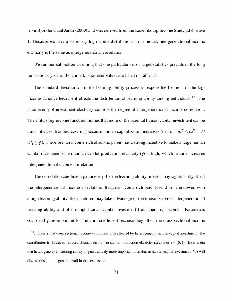
from Bjorklund and Jantti (2009) and was derived from the Luxembourg Income Study(LIS) wave

1. Because we have a stationary log income distribution in our model, intergenerational income

elasticity is the same as intergenerational correlation.

We run our calibration assuming that one particular set of target statistics prevails in the long

run stationary state. Benchmark parameter values are listed in Table 13.

The standard deviation σv in the learning ability process is responsible for most of the log-

income variance because it affects the distribution of learning ability among individuals.13 The

parameter γ of investment elasticity controls the degree of intergenerational income correlation.

The child’s log-income function implies that more of the parental human capital investment can be

transmitted with an increase in γ because human capitalization increases (i.e., h = asγ ≤ asγ′ = h′

if γ≤ γ′). Therefore, an income-rich altruistic parent has a strong incentive to make a large human

capital investment when human capital production elasticity (γ) is high, which in turn increases

intergenerational income correlation.

The correlation coefficient parameter ρ for the learning ability process may significantly affect

the intergenerational income correlation. Because income-rich parents tend to be endowed with

a high learning ability, their children may take advantage of the transmission of intergenerational

learning ability and of the high human capital investment from their rich parents. Parameters

σv, ρ and γ are important for the Gini coefficient because they affect the cross-sectional income

13It is clear that cross-sectional income variation is also affected by heterogeneous human capital investment. The

contribution is, however, reduced through the human capital production elasticity parameter γ ∈ (0,1). It turns out

that heterogeneity in learning ability is quantitatively more important than that in human capital investment. We will

discuss this point in greater detail in the next section

71

distribution. However, the magnitude is ambiguous.14

The three parameters γ,ρ,σv are simultaneously determined within our model in a way that

best matches the statistics in Table 14. In choosing ρ,σv, we choose the stationary learning

ability distribution. As shown in Table 14, our benchmark specification matches target statistics at

the tolerance15 level 10−4.

Suppose the human capital investment is made by a planner such that all children are provided

with the same amount of human capital investment. Cross-sectional income variation in this case is

determined solely by stationary ability variance16, and the intergenerational income correlation is

equivalent to the intergenerational ability correlation.17 Because the intergenerational transmission

of human capital is only made through the transmission of exogenous ability, we may interpret ρ

as a lower bound for the intergenerational correlation. Further, in our benchmark specification,

the direct effect of learning ability correlation explains 20% of the intergenerational correlation

for the U.S. Due to the construction of the model, the intergenerational log-income correlation is

explained more by the ability correlation when countries are more intergenerationally mobile.

3.5 Cross-country Comparison

We calibrate our model for 10 OECD countries. Countries are represented using different param-

eterizations of the model. Specifically, they are described by parameters that characterize human

14In fact, all three parameters simultaneously affect the targets shown in Table 14 to some degree.15We use our criterion function as the average square of the log difference between the model outcomes and the

data targets.16Note that log(y) = log(κ)+ log(a), var(log(y)) = var(log(a)).17E(log(y′) log(y)) = E(log(a′) log(a)) = ρE(log(a)2). Hence, corr(log(y′), log(y)) = ρ.

72

capital production efficiency and the learning ability distribution. In this section, we study how

institutional differences affect the cross-country intergenerational log income correlation as well

as the cross-sectional income Gini.

We assume that the correlation of intergenerational learning abilities is invariant across coun-

tries. First, individuals from all countries are, on average, subject to the same degree of genetic

transmission. Second, given that all parents in each country are assumed to act altruistically toward

their children, the average exogenous environmental effect that potentially affects learning ability

should be similar across individuals in all countries; for example, the effect of social class, reputa-

tion and positive attitudes of parents on children’s learning ability formation may be captured by

the correlation coefficient. Thus, the assumption of the invariant correlation of intergenerational

learning abilities may not be too restrictive; therefore, we take ρ from the U.S. as the benchmark

value for all countries we consider.

Most countries do not have sufficiently long panel data that cover the complete life-cycle in-

come series for at least two generations.18 Although we do not have descriptive statistics for

lifetime income, we do have empirical estimates of intergenerational income elasticity and a cross-

sectional inequality measure (that is, the Gini coefficient).19 We assume these two data statistics

prevail in the long-run steady state and calibrate the remaining two parameters σv,γ.

18The intergenerational income correlation in the empirical literature is generally computed using the proxy lifetime

income variable (i.e., the time average or present discount value of several years of income).19For our data moments, we use the Table Y in Bjorklund and Jantti (2009).

73

3.5.1 Summary of Results

We tabulate the data and model moments, and parameter values in Table 15. Notice that coun-

tries with a high standard deviation σv in the ability process unambiguously have high log-income

Gini values as shown in Figure 13, whereas the standard deviation has a weaker relationship with

intergenerational income persistence. For example, Denmark has a relatively low value of inter-

generational correlation at 0.123 and a relatively high value of σv equal to 0.473. On the other

extreme, the U.K. has a relatively high correlation value at 0.5, with σv equal to 0.4.

Intuitively, as learning ability variance increases, so does the variance of the human capital

holdings. Thus, cross-sectional income inequality, measured by the Gini index, tends to increase.

Intergenerational persistence, however, is significantly affected by country-specific human capital

production efficiency, which is measured by parameter γ in our model. The high value of the effi-

ciency parameter together with random effects can amplify intergenerational income persistence,

as in the U.K. However, a low efficiency parameter with the same degree of learning ability can

suppress intergenerational income persistence, as in Denmark.20

Countries with a high intergenerational correlation have large marginal returns on the per-

unit human capital investment. As shown in Figure 14, the intergenerational income correlation

monotonically increases with the efficiency parameter γ. Consider a country with a high level of

human capital production efficiency (i.e., a high γ). Children from poor families tend to be less

endowed with learning abilities because their parents also have a low level of ability on average.

Given their low incomes, a relatively small human capital investment in these families would be

20See Table 15

74

optimal. Alternatively, children from rich families tend to be endowed from their parents, who

presumably have a high learning ability, with the same high ability. Thus, rich altruistic parents

have incentives to make relatively large human capital investments. Hence, in high-γ societies,

intergenerational income persistence tends to be large, as Figure 14 shows.

As for the impact of the efficiency parameter γ on the cross-sectional income Gini coefficient,

we do not observe much variation in Gini across γ. In other words, the differences in human capital

production efficiency are not quantitatively important in determining cross-sectional inequality.

Why do countries have different levels of human capital production efficiency? In this model,

we assume that there is no direct governmental human capital investment subsidy to households.

However, we assume that the government supports such investments through public education ex-

penditures and various tax rebates on education spending. These types of governmental policies

could be viewed as public human capital investments in the context of our model. Thus, a country

with large public investments could have low marginal returns on private human capital invest-

ment on average, which in turn translates into a low value of the efficiency parameter γ in our

model. Using OECD education spending time-series data, we display the relationship between

intergenerational correlation estimates and the ratio of government education spending to GDP in

Figure 15.

Except for Canada, countries with a high ratio of public education spending to GDP tend to

have a low intergenerational correlation (a low γ21). This figure may provide some implications

for both the quantitative and qualitative enhancement of public education as a tool for a more

intergenerationally mobile society.

21See Figure 14.

75

3.6 Ability Distribution on Intergenerational Mobility

In the previous section, we showed that the learning ability variance σ2v has a quantitatively weaker

relationship with the intergenerational income correlation than the efficiency parameter γ. How-

ever, as shown in Table 15, the overall variance is positively related to the intergenerational corre-

lation. Thus, in this section, we focus on how changes in variance affect the degree of mobility.

When σv is low, the variance of learning ability is low. Therefore, individuals are relatively

homogeneous in their learning ability. In this case, parents’ human capital investment is the main

determinant of children’s earnings capacities. We may therefore expect a high covariance among

intergenerational income but a low variance among cross-sectional income, which yields a low

value for the intergenerational income correlation.

However, when the variation of learning ability is relatively large, the relative income of off-

spring in the cross-sectional distribution may significantly differ from that of parents, whereas

the variance of cross-sectional income is large. In this case, we expect a low intergenerational

correlation with a low intergenerational covariance and a high cross-sectional variance.

From the benchmark parameterization, we show the intergenerational correlation pattern with

respect to σv in Figure 16. The correlation increases slightly when σv increases from 0.1 to 0.3, and

it decreases thereafter. As expected, when learning abilities are relatively homogeneous (i.e., σv up

to 0.4), the intergenerational covariance effect dominates, and the correlation is relatively large. As

abilities become more heterogeneous (i.e., σv greater than 0.4), the cross-sectional variance effect

dominates, and the correlation decreases.

How important is the influence of the ability distribution on the intergenerational log-income

76

correlation? For σv ∈ [0.1,0.7], the intergenerational correlation is within [0.45,0.54]. σv = 0.7

maps onto the stationary log-income variance of 0.8, whereas 0.1 of σv maps onto a log-income

variance at 0.0017.22 Although an increase in σv from 0.1 to 0.7 drastically alters the stationary

cross-sectional log-income variance, corr(log(y′), log(y)) changes only slightly, from 0.45 to 0.54.

Consider an economy in which the variance of the learning ability distribution increases. When

it is relatively small (i.e., a value of up to 0.4 for σv), human capital investment is relatively less

risky in its returns. Thus, income-rich (income-poor) parents of high (low) ability tend to transmit

high (low) human capital together along with their high(low) ability. In this case, a relatively high

intergenerational income correlation is expected. However, when the variance becomes sufficiently

great (i.e., greater than 0.4 of σv), human capital investment becomes riskier because the returns

become more contingent on the randomness of error in the learning ability process. Thus, in this

case, the intergenerational income correlation decreases.

3.7 The Effect of Direct Governmental Human Capital Invest-

ment on Intergenerational Mobility

In Section 3.5, we made the plausible argument that cross-country heterogeneity in public educa-

tion spending may be closely related to the magnitude of the efficiency parameter γ in the human

capital production function. In this section, we ask how intergenerational mobility would change

if individuals became more homogeneous in human capital investment. We consider a direct gov-

ernmental subsidy to human capital investment. Specifically, we focus on the case in which a

22The stationary variance of cross-sectional log-income is 0.36 in our benchmark

77

part of income tax revenue is used to directly subsidize human capital investment in a lump-sum

manner.23

y′ = κa′(s+ g)γ

Once the direct governmental subsidy g is added in the human capital production function

above, each family revises its human capital investment decision depending on its state (y,a),

which in turn influences the intergenerational income correlation. We show the correlation with

respect to the level of subsidy in Figure 17. When the subsidy g increases, the correlation decreases

continuously.

A subsidy up to around 3% of the mean lifetime income does not change the overall investment

behavior of households or the correlation. However, the correlation declines steeply with a sizable

increase in the subsidy of more than 3%. Namely, all households decrease their human capital

investment as the subsidy increases.24 The magnitude of the decline is relatively larger (smaller) if

a household is income-rich (income-poor) because the marginal returns from the human capital in-

vestment are relatively smaller (larger) for income-rich (income-poor) families. With a sufficiently

large subsidy, the role of human capital investment becomes negligible, even in income-poor fam-

ilies. Hence, the correlation declines at a slower pace and attains the minimum bound 0.1 of the

correlation coefficient of the intergenerational learning ability .

Although direct subsidy can reduce the intergenerational log-income correlation, this policy

may not be socially desirable. Clearly, our model is not fit to answer this type of question without

23Notice that the purpose of this exercise is to see the effect of equalizing human capital investment on intergenera-

tional mobility. The government’s budget is therefore not an issue here.24Using the Euler equation, we can easily check that ds

dg < 0

78

a plausible measure of the welfare impact of the change in human capital policy. Nevertheless, this

direct subsidy exercise shows that the intergenerational income correlation marginally declines as

human capital investment equalizes.

3.8 Conclusion

In this paper, we quantify a dynasty version of the BT model and study its implications. When

we apply our model to 10 OECD countries, we find that cross-sectional inequality depends more

on the exogenous ability transmission process than on the human capital investment. However,

intergenerational mobility is heavily influenced by human capital production efficiency. Therefore,

countries with low human capital returns on investment tend to be more intergenerationally mobile.

Given the simple structure of the model, we find that direct human capital investment subsidies

are quite effective in reducing the intergenerational income correlation. For instance, a subsidy of

10% of mean income reduces the correlation from 0.51 to 0.2, whereas a subsidy of 20% reaches

the minimum bound of 0.1. Hence, intergenerational income links can be substantially reduced by

subsidy policies or similar measures.

The model in our paper does not have a general equilibrium structure, so it is not well suited

to analyze the welfare consequences of subsidizing household human capital investment. How-

ever, the intergenerational income correlation marginally decreases with increasing subsides as

Figure 17 shows, so it would be interesting to extend our model to incorporate the government’s

budget to assess the optimal subsidy level that would maximize social mobility, and to determine

some criteria for social welfare.

79

Finally, one policy implication of the model is that the government should subsidize children

from poor families so they may have more opportunities to be exposed to environments conducive

to learning, which would enhance their chances of economic success. This type of normative

statement may be justified in view of the BT strain of human capital investment theory because the

marginal returns from subsidies are relatively larger for children from poor families. However, we

do not yet know the extent to which the redistribution of resources through a subsidy is welfare-

maximizing.

80

Bibliography

[1] AGHION, P., AND HOWITT, P. Endogenous Growth Theory. MIT Press, 1998.

[2] ALBRECHT, J., NAVARRO, L., AND VROMAN, S. The effects of labor market policies in an

economy with an informal sector. Economic Journal 119 (2009), 1105–1129.

[3] ALTONJI, J. G., AND DUNN, T. A. The effects of family characteristics on the return to

education. Review of Economics and Statistics 78 (1996), 692–704.

[4] AMARAL, P., AND QUINTIN, E. A competitive model of the informal sector. Journal of

Monetary Economics 53(7) (2006), 1541–1553.

[5] ANDOLFATTO, D. Business cycles and laobr-market search. American Economic Review

86(1) (1996), 112–32.

[6] BECKER, G., AND TOMES, N. An equilibrium theory of the distribution of income and

intergenerational mobility. Journal of Political Economy 87 (1979), 1153–89.

[7] BECKER, G., AND TOMES, N. Human capital and the rise and fall of families. Journal of

Labor Economics 4 (1986), S1–S39.

81

[8] BEN-PORATH, Y. The production of human capital and the life cycle of earnings. Journal

of Political Economy 75 (1967), 352–365.

[9] BJORKLUND, A., AND JANTTI, M. Intergenerational mobility of socio-economic status in

comparative perspective. Nordic Journal of Political Economy 26 (2000), 3–32.

[10] BJORKLUND, A., AND JANTTI, M. Intergenerational Income Mobility and the Role of

Family Background. Oxford University Priess, 2009, ch. 20.

[11] BJORKLUND, A., JANTTI, M., AND SOLON, G. Influences of Nature and Nurture on Earn-

ings Variation: A Report on a Study of Various Sibling Types in Sweden. Russell Sage Foun-

dation, 2003.

[12] BLANDEN, J., GREGG, P., AND MACMILLAN, L. Accounting for intergenerational income

persistence: Noncognitive skills, ability and education. Economic Journal 117 (2007).

[13] BRATSBERG, B., ROED, K., RAAUM, O., NAYLOR, R., JANTTI, M., ERIKSSON, T., AND

OSTERBACKA, E. Nonlinearities in intergenerational earnings mobility: Consequences for

cross-country comparisions. Economic Journal 117 (2007).

[14] BRAVO-ORGETA, C., AND LEDERMAN, D. Agriculture and national welfare around the

world: Causality and international heterogeneity since 1960. ESTUDIOS DE ECONOMIA

31(002) (2004).

[15] BURDETT, K., AND MORTENSEN, D. Wage differentials, employer size and unemployment.

International Economic Review 39 (1998), 257–73.

82

[16] CARNEIRO, P., HANSEN, K. T., AND HECKMAN, J. J. Removing the veil of ignorance in

assessing the distributional impacts of social policies. Swedish Economic Policy Review 8

(2001), 273–301.

[17] CORAK, M. Do poor children become poor adults? lessons from a cross country comparision

of generational earnings mobility. IZA Discussion Paper No. 1993 (2006).

[18] CORAK, M., AND HEISZ, A. The intergenerational earnings and income mobility of cana-

dian men: Evidence from longitudinal income tax data. Journal of Human Resources 34/3

(1999).

[19] CORCORAN, M., GORDON, R., LAREN, D., AND SOLON, G. A longitudinal analysis of

sibling correlations in economic status. The Journal of Human Resources 26 (1991), 509–

534.

[20] CORCORAN, M., GORDON, R., LAREN, D., AND SOLON, G. A longitudinal analysis of

sibling correlations in economic status. The Journal of Human Resources 26 (1991), 509–

534.

[21] D’ADDIO, A. C. Intergenerational transmission of disadvantage: Mobility or immobility

across generations? a review of the evidence for oecd countries. OECD SOCIAL , EMPLOY-

MENT AND MIGRATION WORKING PAPERS (2007).

[22] DANIELS, M., DEVLIN, B., AND ROEDER, K. Of Genes and IQ. New York: Springer-

Verlag, 1997.

83

[23] EARLE, J., AND SAKOVA, Z. Business start-ups or disguised unemployment? evidence on

the character of self-employment from transition economies. Labour Economics 7(5) (2000),

575–601.

[24] EROSA, A., AND KORESHKOVA, T. Progressive taxation in a dynastic model of human

capital. Journal of Monetary Economics 54(3) (2007), 667–685.

[25] FIELDS, G. Rural-urban migration, urban unemployment and underemployment, and job-

search activity in ldc’s. Journal of Development Economics 2 (1975), 165–187.

[26] FLINN, C. Minimum wage effects on labor market outcomes under search, matching and

endogenous contact rates. Econometrica 74 (2006), 1013–1062.

[27] GILES-SAINT, P. Dual Labor Markets. Cambridge MIT Press, 1996.

[28] GONG, X., VAN SOEST, A., AND VILLAGOMEZ, E. Mobility in the urban labor market:

A panel data analysis for mexico. Economic Development and Cultural Change 53 (2004),

1–36.

[29] GRAWE, N. Reconsidering the use of nonlinearities in intergenerational earnings mobility as

a test for credit constraints. Journal of Human Resources 39/3 (2004).

[30] GUTIERREZ, C., PACI, P., AND PARK, B. S. Quantifying the impact of financial crisis on a

multi-sector labor market. World Bank mimeo (2009).

[31] HAIDER, S., AND SOLON, G. Life-cycle variation in the association between current and

lifetime earnings. American Economic Review Forthcoming (2006).

84

[32] HARDING, D. J., JENCKS, C., LOPOO, L. M., AND MAYER, S. E. The Changing Effect

of Family Background on the Incomes of American Adults in Unequal Chances : Family

Background and Economic Success. Russell Sage Foundation : Princeton University Press,

2005.

[33] HASSLER, J., RODRIGUES, J., AND ZEIRA, J. Inequality and mobility. Journal of Economic

Growth 12/3 (2007).

[34] HD, AND PREM. How should labor market policy respond to the financial crisis? World

Bank (2009).

[35] HECKMAN, J. J., AND CARNEIRO, P. Human Capital Policy. The MIT Press, 2002.

[36] HUGGETT, M., VENTURA, G., AND YARON, A. Human capital and earnings distribution

dynamics. Journal of Monetary Economics 53 (2006), 265–90.

[37] HUGGETT, M., VENTURA, G., AND YARON, A. Sources of lifetime inequality. Working

Paper (2010).

[38] ISLAM, I., AND VERICK, S. The great recession of 2008-2009: Causes, consequences and

policy responses. IZA Discussion Paper Series No. 4934 (2010).

[39] KEANE, M. P., AND WOLPIN, K. I. The career decisions of young men. Journal of Political

Economy 105 (1997), 473–522.

85

[40] LALL, S. V., SELOD, H., AND SHALIZI, Z. Rural-urban migration in developing countries:

A survey of theoretical predictions and empirical findings. World Bank Research Working

Paper (2006).

[41] LEE, C.-I., AND SOLON, G. Trends in intergenerational income mobility. Review of Eco-

nomics and Statistics 91 (2009), 766–772.

[42] LOCHNER, L., AND MONGE-NARANJO, A. Human capital formation with endogenous

credit constraints. NBER Working Papers 8815 (2002).

[43] MAGNAC, T. Segmented or competitive labor markets. Econometrica 59 (1991), 165–87.

[44] MALONEY, W. Does informality imply segmentation in urban labor markets? evidence from

sectoral transitions in mexico. World Bank Economic Review 13 (1999), 275–302.

[45] MALONEY, W. Informality revisited. World Development 32(7) (2004), 1159–1178.

[46] MALONEY, W., AND BOSCH, M. Cyclical movements in unemployments and informality

in developing countries. World Bank Policy Research Working Papers No. 4648 (June 2008).

[47] MALONEY, W. F. Are labor markets in developing countries dualistic? Policy Research

Working Paper (1998).

[48] MANNING, A. Monopsony in Motion. Princeton University Press, 2003.

[49] MAZUMDER, B. Fortunate sons: New estimates of intergenerational mobility in the united

states using social security earnings data. Review of Economics and Statistics 87(2) (2005),

235–255.

86

[50] MORTENSEN, D., AND PISSARIDES, C. Technological progress, job creation and job de-

struction. Review of Economic Dynamics 1 (1994), 133–53.

[51] OI, W. Y., AND IDSON, T. L. Firm Size and Wages. Elsevier Science B.V., 1999, ch. 33,

pp. 2165–2214.

[52] PACI, P., REVENGA, A., AND RIJKERS, B. Coping with crises, why and how to protect

employment and informality in developing countries. World Bank Policy Research Working

Paper, No. 5094 (2009).

[53] PISSARIDES, C. Equilibrium Unemployment Theory. Cambridge MIT Press, 2000.

[54] POVERTY TEAM, W. B. O. J. Labor market trends in indonesia: Indonesia jobs report.

Working Paper (2009).

[55] PRATAP, S., AND QUINTIN, E. Are labor markets segmented in developing countries? a

semiparametric approach. European Economic Review 50(7) (2006), 1817–1841.

[56] RESTUCCIA, D., AND URRUTIA, C. Intergenerational persistence of earnings: The role of

early and college education. American Economic Review (2004), 1354–1378.

[57] ROSENZWEIG, M. R. Labor Markets in Low-Income Countries. Elsevier Science B.V., 1988,

ch. 15, pp. 713–762.

[58] SATCHI, M., AND TEMPLE, J. Labor markets and productivity in developing countries.

Review of Economic Dynamics 12 (2009), 183–204.

87

[59] SCHNEIDER, F., AND ENSTE, D. Shadow economies: Size, causes, and consequeces. Jour-

nal of Economic Literature 38 (2000), 77–114.

[60] SMITH, J. P., THOMAS, D., FRANKENBERG, E., BEEGLE, K., AND TERUEL, G. Wages,

employment and economic shocks: Evidence from indonesia. Journal of Population Eco-

nomics 15(1) (2002), 161–193.

[61] SOLON, G. Intergenerational income mobility in the united states. The American Economic

Review 82 (1992), 393–408.

[62] SOLON, G. Intergenerational Mobility In the Labor Market. Elsevier Science B.V., 1999.

[63] SOLON, G. A Model of Intergenerational Mobility Variation over Time and Place. Cam-

bridge University Press, 2004.

[64] STROBL, E., AND BYRNE, D. Defining unemployment in developing countries: Evidence

from trinidad and tobago. Journal of Development Economics 73(1) (2004), 465–476.

[65] TAUBMAN, P., AND WACHTER, M. L. Segmented Labor Markets. Elsevier Science Pub-

lishers, 1986.

[66] UDALL, A. T., AND SINCLAIR, S. The ’luxuary unemployment’ hypothesis: A review of

recent evidence. World Development 10 (1982), 49–62.

[67] YAMADA, G. Urban informal employment and self-employment in developing countries:

Theory and evidence. Economic Development and Cultural Change 44 (1996), 289–314.

88

Appendix A: Definitions of Unemployment, Informality and For-

mality

How do we assign workers in the data to the four labor market states25? We divide workers from the

EMNV into several occupational categories: wage workers in the formal sector, wage workers in

the informal sector, family enterprise workers, and the individually self-employed and employers,

distinguishing between those workers in primary sector activities (agriculture, hunting, forestry

and fishing) and those outside of primary sector activities.26 For each of these categories, we

compute average earnings, poverty rates and the share of low earners among each category.

We attempt to find categories of workers whose earnings are distributed at the low quantiles and

high poverty incidence rates. For Nicaragua, this method assigns family enterprise workers, indi-

vidually self-employed and informal wage workers outside of agriculture to the low productivity

informal sector. Formal wage workers are assigned to the high productivity sector, and agricultural

workers (not agricultural employers) are all assigned to the agricultural sector. Employers in both

agriculture and non-agriculture are left out all together. We believe that they are better understood

as firms, rather than workers.

We can define unemployment in two different ways. The first is to use a narrow definition of

25These states are unemployment, employment in the urban formal and informal sectors, and employment in the

agricultural sector.26Employers are defined as self-employed workers who employ at least one paid non-family member at work. The

individually self-employed are defined as those who are self-employed and do not work with other family members

and do not employ other workers, and family enterprise workers are defined as the self-employed who work with other

family members, whether paid or unpaid, in the same enterprise and do hire non-family workers.

89

unemployment in which only those actively seeking jobs are classified as unemployed workers.

However, it is well known that the use of this definition is limited for developing countries. As

labor markets are not well developed, job search mechanisms are mostly informal and are unlikely

to be captured in the traditional labor force questionnaires. It is common in developing countries

that a large number of non-employed workers who are not actively searching for a job would take

a job if offered, but these non-employed workers are classified as ”discouraged” in the standard

definition. In addition, many inactive workers are temporarily inactive, waiting for harvests or

other seasonal activities. These features often merit a ”broader” definition of unemployment that

takes into account discouraged and temporarily inactive workers.

Using the household survey, we classify workers as unemployed if they are temporarily in-

active, discouraged or inactive for other reasons, and we look at the transition rates from these

states to employment. We find that people classified as discouraged or as temporarily inactive have

transition rates into and out of employment similar to those classified as unemployed under the

narrow definition. This suggests that those temporarily inactive and those classified as discouraged

workers are not very different from unemployed workers and as such, should be counted among

the unemployed. This evidence suggests that for Nicaragua, the broad definition of unemploy-

ment better represents the status of the idle labor force. While the narrow unemployment rates are

around 4%, the broad rate is 12%, as shown in Table 1.

90

Appendix B: Calibration

Step 1: Calibration of the Distribution of Skill and Idiosyncratic Shocks to the Formal Sector

In the first step, we specify the parameters of the shock process (G(y)) and those of the distribu-

tion of skills (F(y)). We assume that the shock process is described by a uniform distribution with

a support of [0,y]. In other words, when a shock arrives, a new level of productivity of a worker of

type y lies between 0 and y, with an equal probability of ending up anywhere in this support. The

uniform distribution is completely specified by its support.

We assume that workers’ skill is distributed according to a β-distribution F(y), and we proxy

the skill by the level of education normalized by its maximum level. The β-distribution is flexible,

with a finite support between [0,1]. It can display a broad range of shapes depending on its two

parameters abeta and bbeta. It can be skewed or have the standard bell shape.

Let abeta and bbeta denote two parameters. The mean and variance of the β-distribution are

given by

E[y] =abeta

abeta +bbeta

var[y] =abeta

(abeta +bbeta)2 (abeta +bbeta +1)

We use the mean years of education and its variance from the EMNV survey to calibrate the

two parameters in the distribution of skill. Since our distribution has the support of [0,1], we

normalize the distribution by dividing individual years of education by the highest level displayed

in the data. The mean years of education among the active working age population in Nicaragua

91

is 4.59 years, with a standard deviation of 4.3 years. The maximum level of education observed

among those in the labor force is 19 years. This means that we set

abeta

abeta +bbeta= 0.302,

abeta

(abeta +bbeta)2(abeta +bbeta +1)= 0.0529,

where 0.302 and 0.529 are the mean and variance of the normalized level of education.

Step 2: Calibration of the Parameters Determining Earnings in the Informal Sector and

in Agriculture.

The earnings in agriculture are given by the following average product of labor:

ya = Aalγ−1a . (1)

We estimate the labor elasticity (γ) with longitudinal data for agricultural production and em-

ployment from 1961 to 2005. Data on agricultural output (Ya) come from the Central Bank of

Nicaragua. To have a long enough series of agricultural employment, we use the household survey

(EMNV) from 2001 and 2005 as well as the data from the FAO for the working age population in

the agricultural sector. Using these data, we estimate that

logYa = c+ γ logLa.

The estimate of γ is 0.628. Because income from agriculture is given by (1), we can compute

Aa. Using the household survey, we calculate average income in the agricultural sector, (ya), and

92

the share of workers in agriculture, la. The average income in agriculture is $10,717 cordobas, and

la is 27.1%, as shown in Table 1. This allows us to compute Aa.

Finally, we find the average income in the informal sector (y0 = 12,519 cordobas).

Step 3: Calibration of Other Parameters in the Model

We calibrate our model to determine the remaining parameters by matching the share of work-

ers in the formal and informal sectors (N0 and N1, respectively), the share of workers in the agri-

cultural sector (Na), the average wage (W ), and the duration of formal and informal jobs (d1 and

d0, respectively).

We can derive explicit expressions for those targets from our model, and the data values for

those targets are readily observed from the household survey. Using these target values, we com-

pute the values of λ,δ,α,m(θ) and A1. Next, we determine the migration cost (M) and the cost

of a vacancy (c) using the no-migration and free-entry conditions, respectively. In what follows,

we describe this calibration step in greater detail. We first show the analytic expressions for the

targets.

Our model implies that informal sector workers face the job destruction rate δ. Because we

are assuming that the rate follows a Poisson process, each employed worker in the informal sector

is expected to hold his job for 1/δ periods. In other words, the duration of a bad job is given

by d0 = 1/δ. We can calculate the duration of informal jobs from the household survey, and this

allows us to back out δ.

The share of the population employed in the informal sector is given by

93

n0 =∫ 1

yrn0 (y) f (y)dy, (2)

with n0(y) taking different values depending on the type of worker. In other words, for y < y∗,

n0(y) =α

δ+α,

for y∗ < y < y∗∗,

n0 (y) =αλG(R(y))

λ(δ+α)G(R(y))+δm(θ)G(y),

and for y > y∗∗

n0(y) = 0.

The share of the population employed in the formal sector is given by

n1 =∫ 1

yrn1 (y) f (y)dy, (3)

with n1(y) taking different values depending on the worker type. For y < y∗,

n1(y) = 0,

for y∗ < y < y∗∗,

n1(y) =δm(θ)G(y)

λ(δ+α)G(R(y))+δm(θ)G(y),

and for y > y∗∗,

n1(y) =m(θ)G(y)

λG(R(y))+m(θ)G(y).

94

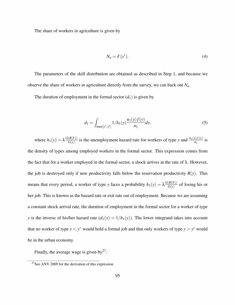
The share of workers in agriculture is given by

Na = F(yr). (4)

The parameters of the skill distribution are obtained as described in Step 1, and because we

observe the share of workers in agriculture directly from the survey, we can back out Na.

The duration of employment in the formal sector (d1) is given by

d1 =∫

max[y∗,yr]1/h1(y)

n1(y) f (y)n1

dy, (5)

where h1(y) = λG(R(Y ))

G(y) is the unemployment hazard rate for workers of type y and n1(y) f (y)n1

is

the density of types among employed workers in the formal sector. This expression comes from

the fact that for a worker employed in the formal sector, a shock arrives at the rate of λ. However,

the job is destroyed only if new productivity falls below the reservation productivity R(y). This

means that every period, a worker of type y faces a probability h1(y) = λG(R(Y ))

G(y) of losing his or

her job. This is known as the hazard rate or exit rate out of employment. Because we are assuming

a constant shock arrival rate, the duration of employment in the formal sector for a worker of type

y is the inverse of his/her hazard rate (d1(y) = 1/h1(y)). The lower integrand takes into account

that no worker of type y < y∗ would hold a formal job and that only workers of type y > yr would

be in the urban economy.

Finally, the average wage is given by27:

27See ANV 2009 for the derivation of this expression

95

W =∫ 1

y∗Ω(y)

n1(y) f (y)n1

dy (6)

Ω(y) = w(y,y)G(R(y))

G(y)+

∫ y

R(y)w(x,y)

g(x)G(y)

dx.

We use the resulting value m(θ) together with the predefined values of ρ = 1/2 and ζ = 1 to

find the value of θ by m(θ) = ζθρ. We now can use the free entry condition (1.22) to back out the

cost of posting a vacancy c. Once we know θ, we can use the expression for unemployment to find

the implied vacancy rate in the economy.

96

Appendix C : Computation Procedure in Chapter 3

We solve the dynamic programming problem using a collocation method. Because our value func-

tion is continuous on a compact, convex interval, we can approximate the value function with

polynomials. We use Chebychev polynomials for our basis functions.28

First we convert AR(1) learning ability into a discrete Markov process using Tauchen’s method.

We choose five discrete points and use the transition matrix to indicate conditional probability

weights. Next, we approximate the value function using n basis functions at n collocation nodes.

We choose 100 nodes and thus the 99th degree of Chebychev polynomial function. Because the

polynomial approximant behaves strangely at extrapolated points, we must choose an adequately

large state interval. We choose the interval [1,1000] for our benchmark model. The maximum

approximation error for our benchmark specification is about 0.4× 10−3 and becomes less than

10−4 for a wide range of the specified interval.

The computational procedure is as follows.

Step 1 Guess a set of parameters γ,ρ,σv.

Step 2 Approximate the policy function for each level of learning ability

Step 3 Guess F0(log(y), log(a))

Step 4 If F0 converges to the stationary distribution F , the iteration stop. Otherwise, repeat the

process, starting with Step 1.28It is well known that Chebychev-node polynomial interpolants are relatively accurate given their low approxima-

tion errors (see Rivlin’s theorem), and even with high-order polynomial approximants, Chebychev polynomials are

quite accurate and computationally efficient (Fackler, 2002).

97

We fix β = ( 11+0.04)

20. Other parameters in step 1 are determined within the model as de-

scribed in section 4. In step 2, we approximate the value function using the Chevyshev polyno-

mial, whereas the policy function is computed using the policy function iteration algorithm. For

this computational procedure, we use the dynamic programming toolbox developed by Miranda

and Fackler (2002).

In Step 3, we first generate the learning ability paths for 1000 simulation periods using the

stationary log(a) distribution and the AR(1) process. We convert the continuous values to discrete

ones (i.e., a discrete approximation of the ability paths). Next, we choose an arbitrary log(y)

distribution with a large number of observations.

By design, the distribution of learning ability is stationary. Given the policy function computed

in step 2, we generate a large number of observations (yi,ai)Ni=1, and we generate a simulation us-

ing the policy function spline while computing var(log(y)), Gini(log(y)), and corr(log(y), log(y′)).

If those moments converge to the data moments, the process is complete. Otherwise, we repeat the

process, starting from step 1.

98

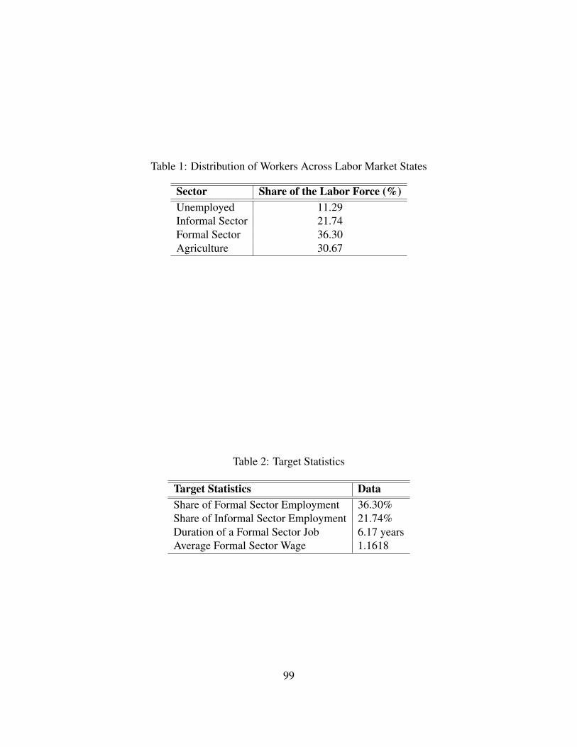
Table 1: Distribution of Workers Across Labor Market States

Sector Share of the Labor Force (%)Unemployed 11.29Informal Sector 21.74Formal Sector 36.30Agriculture 30.67

Table 2: Target Statistics

Target Statistics DataShare of Formal Sector Employment 36.30%Share of Informal Sector Employment 21.74%Duration of a Formal Sector Job 6.17 yearsAverage Formal Sector Wage 1.1618

99

OtherParam

eterV

alueParam

eterofSkillDistribution

aβ

0.7914Param

eterofSkillDistribution

bβ

1.9621TechnologicalParam

eterofFormalSectorProduction

FunctionA

12.8812

TechnologicalParameterofA

griculturalProductionFunction

Aa

0.3476Fixed

Income

fromInform

alSectory0

0.9767O

utputElasticity

ofEm

ploymentin

Agriculture

γ0.628

ShockA

rrivalRate

inForm

alSectorλ

0.2342Shock

ArrivalR

atein

InformalSector

δ0.176

ArrivalR

ateofInform

alSectorEm

ploymentO

pportunitiesα

0.4395M

igrationC

ostM

0.3745C

ostofPostinga

Vacancy

c0.4163

Table3:C

alibratedParam

eters

100

Oth

erPa

ram

eter

Val

ueA

vera

geIn

com

ein

Agr

icul

ture

y a0.

5391

Ave

rage

Inco

me

inFo

rmal

Sect

or(a

vera

gew

age)

y 1=

W1.

1618

Une

mpl

oym

entR

ate

u11

.29%

Thr

esho

ldL

evel

ofSk

ills

requ

ired

tom

igra

teyr

0.11

7T

hres

hold

Lev

elof

Skill

sfo

rInf

orm

alSe

ctor

Sear

chy∗

0.18

81ye

ars

Thr

esho

ldL

evel

ofSk

ills

forF

orm

alSe

ctor

Sear

chy∗∗

0.45

1

Tabl

e4:

Ben

chm

ark

Val

ues

ofE

ndog

enou

sV

aria

bles

101

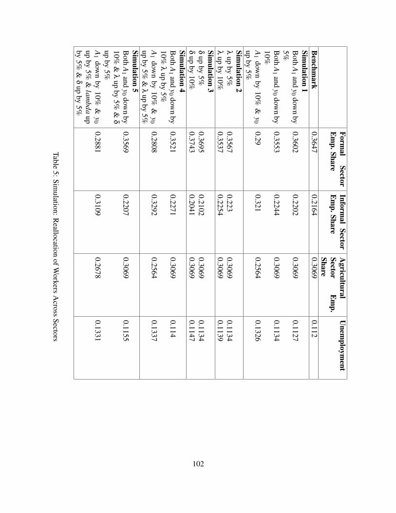
Formal

SectorE

mp.Share

Informal

SectorE

mp.Share

Agricultural

SectorE

mp.

Share

Unem

ployment

Benchm

ark0.3647

0.21640.3069

0.112Sim

ulation1

Both

A1

andy0

down

by5%

0.36020.2202

0.30690.1127

Both

A1

andy0

down

by10%

0.35530.2244

0.30690.1134

A1

down

by10%

&y0

upby

5%0.29

0.3210.2564

0.1326

Simulation

2λ

upby

5%0.3567

0.2230.3069

0.1134λ

upby

10%0.3537

0.22540.3069

0.1139Sim

ulation3

δup

by5%

0.36950.2102

0.30690.1134

δup

by10%

0.37430.2041

0.30690.1147

Simulation

4B

othA

1and

y0dow

nby

10%λ

upby

5%0.3521

0.22710.3069

0.114

A1

down

by10%

&y0

upby

5%&

λup

by5%

0.28080.3292

0.25640.1337

Simulation

5B

othA

1and

y0dow

nby

10%&

λup

by5%

&δ

upby

5%

0.35690.2207

0.30690.1155

A1

down

by10%

&y0

upby

5%&

lambda

upby

5%&

δup

by5%

0.28810.3109

0.26780.1331

Table5:Sim

ulation:Reallocation

ofWorkers

Across

Sectors

102

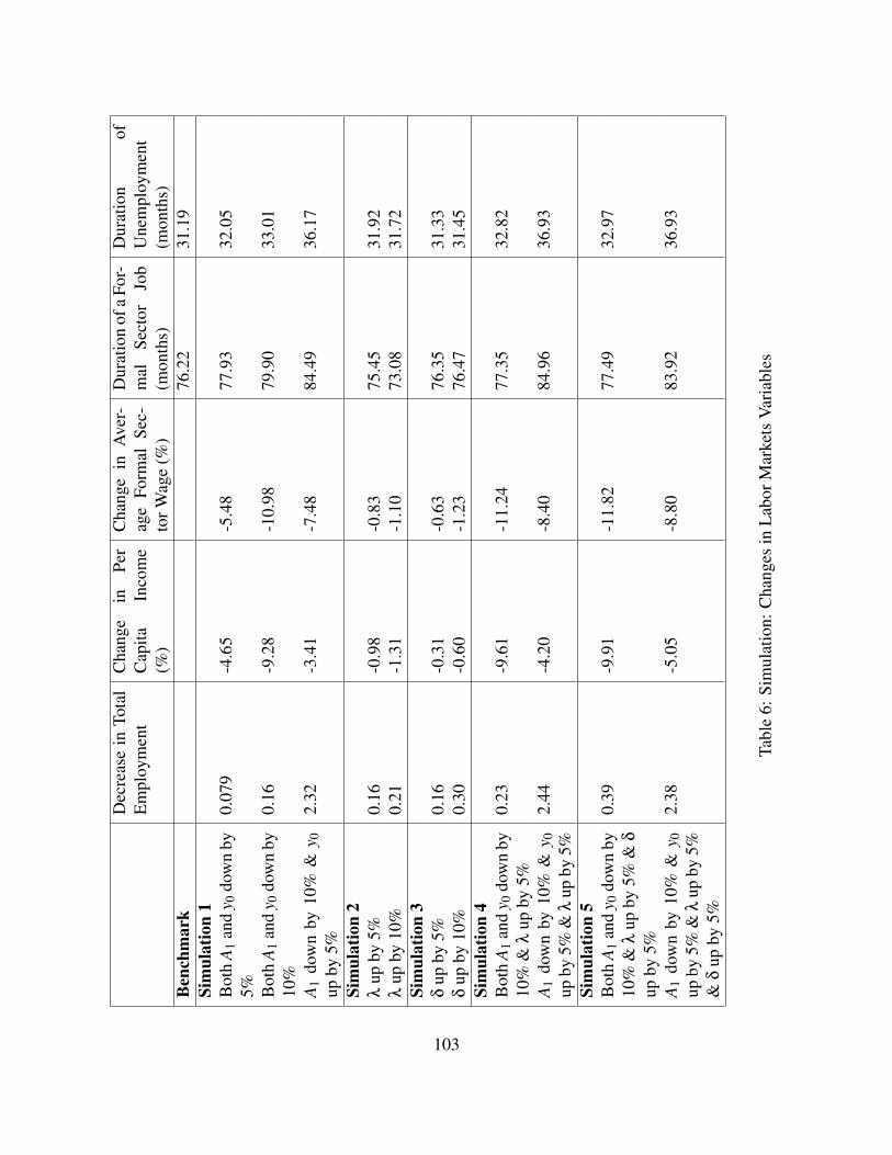
Dec

reas

ein

Tota

lE

mpl

oym

ent

Cha

nge

inPe

rC

apita

Inco

me

(%)

Cha

nge

inA

ver-

age

Form

alSe

c-to

rWag

e(%

)

Dur

atio

nof

aFo

r-m

alSe

ctor

Job

(mon

ths)

Dur

atio

nof

Une

mpl

oym

ent

(mon

ths)

Ben

chm

ark

76.2

231

.19

Sim

ulat

ion

1B

oth

A1

and

y 0do

wn

by5%

0.07

9-4

.65

-5.4

877

.93

32.0

5

Bot

hA

1an

dy 0

dow

nby

10%

0.16

-9.2

8-1

0.98

79.9

033

.01

A1

dow

nby

10%

&y 0

upby

5%2.

32-3

.41

-7.4

884

.49

36.1

7

Sim

ulat

ion

2λ

upby

5%0.

16-0

.98

-0.8

375

.45

31.9

2λ

upby

10%

0.21

-1.3

1-1

.10

73.0

831

.72

Sim

ulat

ion

3δ

upby

5%0.

16-0

.31

-0.6

376

.35

31.3

3δ

upby

10%

0.30

-0.6

0-1

.23

76.4

731

.45

Sim

ulat

ion

4B

oth

A1

and

y 0do

wn

by10

%&

λup

by5%

0.23

-9.6

1-1

1.24

77.3

532

.82

A1

dow

nby

10%

&y 0

upby

5%&

λup

by5%

2.44

-4.2

0-8

.40

84.9

636

.93

Sim

ulat

ion

5B

oth

A1

and

y 0do

wn

by10

%&

λup

by5%

&δ

upby

5%

0.39

-9.9

1-1

1.82

77.4

932

.97

A1

dow

nby

10%

&y 0

upby

5%&

λup

by5%

&δ

upby

5%

2.38

-5.0

5-8

.80

83.9

236

.93

Tabl

e6:

Sim

ulat

ion:

Cha

nges

inL

abor

Mar

kets

Var

iabl

es

103

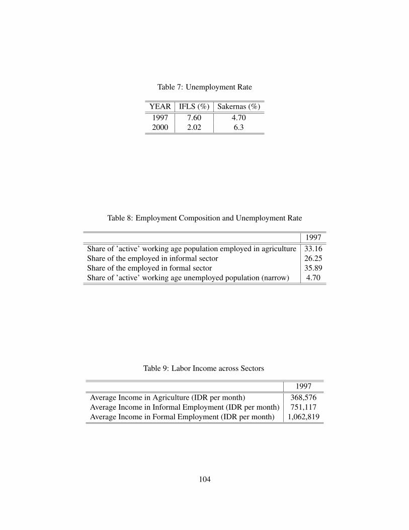
Table 7: Unemployment Rate

YEAR IFLS (%) Sakernas (%)1997 7.60 4.702000 2.02 6.3

Table 8: Employment Composition and Unemployment Rate

1997Share of ’active’ working age population employed in agriculture 33.16Share of the employed in informal sector 26.25Share of the employed in formal sector 35.89Share of ’active’ working age unemployed population (narrow) 4.70

Table 9: Labor Income across Sectors

1997Average Income in Agriculture (IDR per month) 368,576Average Income in Informal Employment (IDR per month) 751,117Average Income in Formal Employment (IDR per month) 1,062,819

104

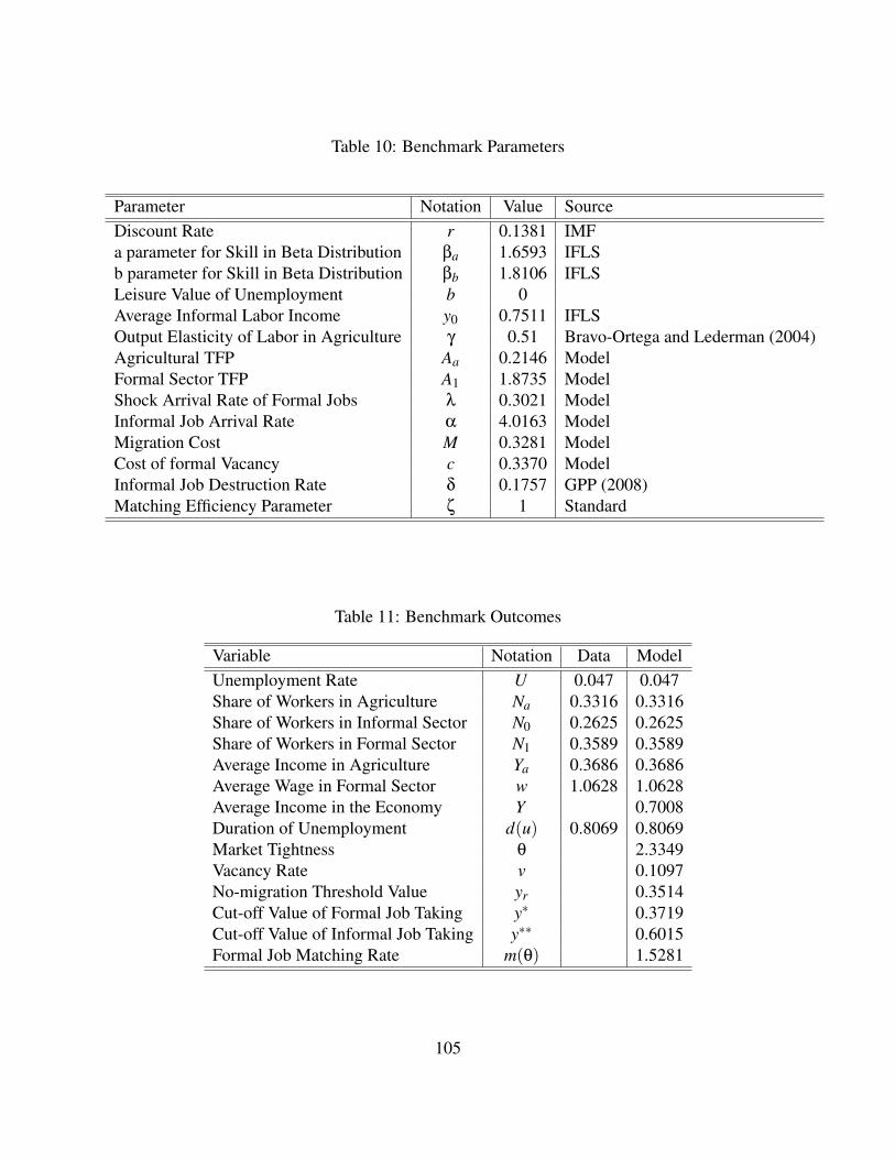
Table 10: Benchmark Parameters

Parameter Notation Value SourceDiscount Rate r 0.1381 IMFa parameter for Skill in Beta Distribution βa 1.6593 IFLSb parameter for Skill in Beta Distribution βb 1.8106 IFLSLeisure Value of Unemployment b 0Average Informal Labor Income y0 0.7511 IFLSOutput Elasticity of Labor in Agriculture γ 0.51 Bravo-Ortega and Lederman (2004)Agricultural TFP Aa 0.2146 ModelFormal Sector TFP A1 1.8735 ModelShock Arrival Rate of Formal Jobs λ 0.3021 ModelInformal Job Arrival Rate α 4.0163 ModelMigration Cost M 0.3281 ModelCost of formal Vacancy c 0.3370 ModelInformal Job Destruction Rate δ 0.1757 GPP (2008)Matching Efficiency Parameter ζ 1 Standard

Table 11: Benchmark Outcomes

Variable Notation Data ModelUnemployment Rate U 0.047 0.047Share of Workers in Agriculture Na 0.3316 0.3316Share of Workers in Informal Sector N0 0.2625 0.2625Share of Workers in Formal Sector N1 0.3589 0.3589Average Income in Agriculture Ya 0.3686 0.3686Average Wage in Formal Sector w 1.0628 1.0628Average Income in the Economy Y 0.7008Duration of Unemployment d(u) 0.8069 0.8069Market Tightness θ 2.3349Vacancy Rate v 0.1097No-migration Threshold Value yr 0.3514Cut-off Value of Formal Job Taking y∗ 0.3719Cut-off Value of Informal Job Taking y∗∗ 0.6015Formal Job Matching Rate m(θ) 1.5281

105

Table 12: Avg. Education by the Model and Data Observation

Data ModelAvg. Education in Agricultural Sector 5.44 3.3768Avg. Education in Informal Employed Workers 6.61 7.5417Avg. Education for Formal Employed Workers 9.01 11.2506Avg. Education for Unemployed Workers 8.68 10.9311

Table 13: Benchmark Parameters

β γ ρ σv

0.4564 0.475 0.1 0.5

Table 14: Target and Model Moments in Benchmark Case

Moment Target Modelcorr(log(y′), log(y)) 0.5 0.51

var(log(y)) 0.36 0.356Gini(log(y)) 0.301 0.31

106

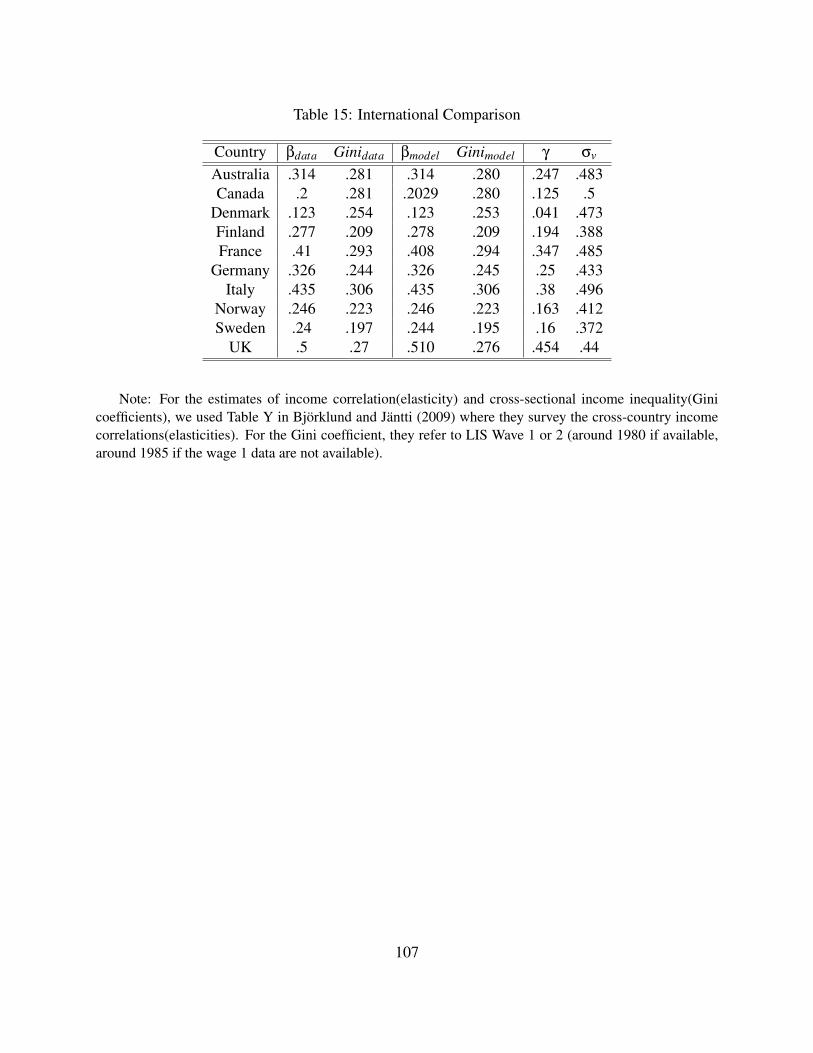
Table 15: International Comparison

Country βdata Ginidata βmodel Ginimodel γ σv

Australia .314 .281 .314 .280 .247 .483Canada .2 .281 .2029 .280 .125 .5

Denmark .123 .254 .123 .253 .041 .473Finland .277 .209 .278 .209 .194 .388France .41 .293 .408 .294 .347 .485

Germany .326 .244 .326 .245 .25 .433Italy .435 .306 .435 .306 .38 .496

Norway .246 .223 .246 .223 .163 .412Sweden .24 .197 .244 .195 .16 .372

UK .5 .27 .510 .276 .454 .44

Note: For the estimates of income correlation(elasticity) and cross-sectional income inequality(Ginicoefficients), we used Table Y in Bjorklund and Jantti (2009) where they survey the cross-country incomecorrelations(elasticities). For the Gini coefficient, they refer to LIS Wave 1 or 2 (around 1980 if available,around 1985 if the wage 1 data are not available).

107

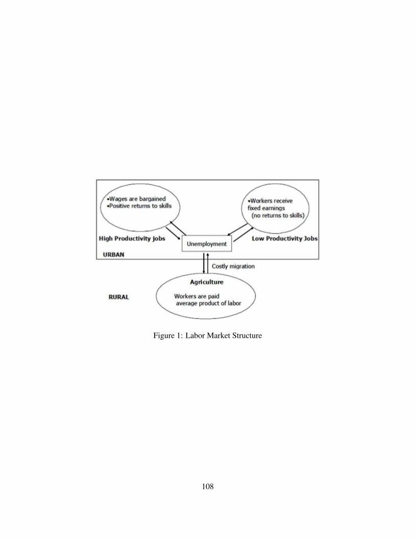
Figure 1: Labor Market Structure

108

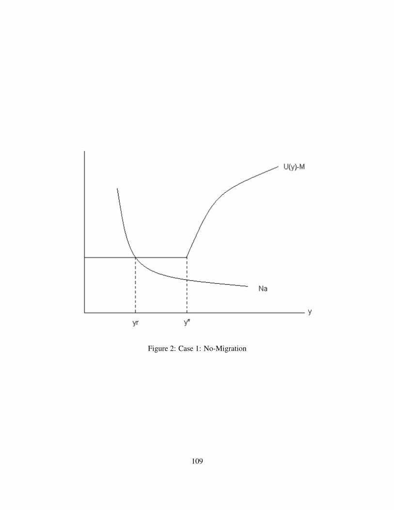
Figure 2: Case 1: No-Migration

109

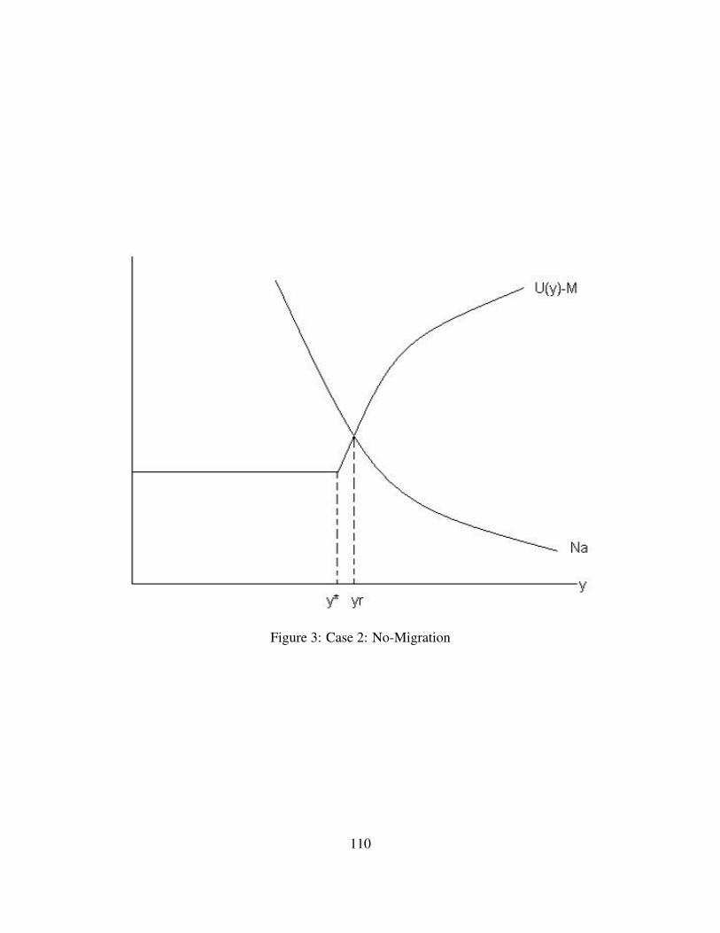
Figure 3: Case 2: No-Migration

110

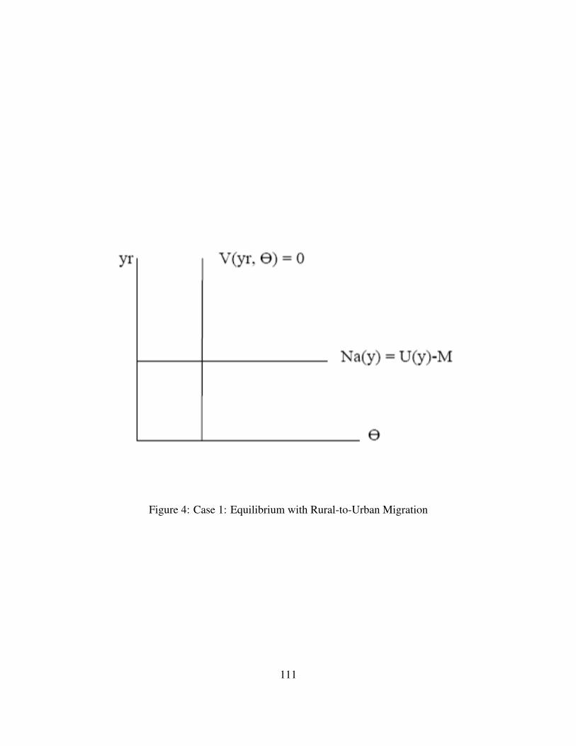
Figure 4: Case 1: Equilibrium with Rural-to-Urban Migration

111

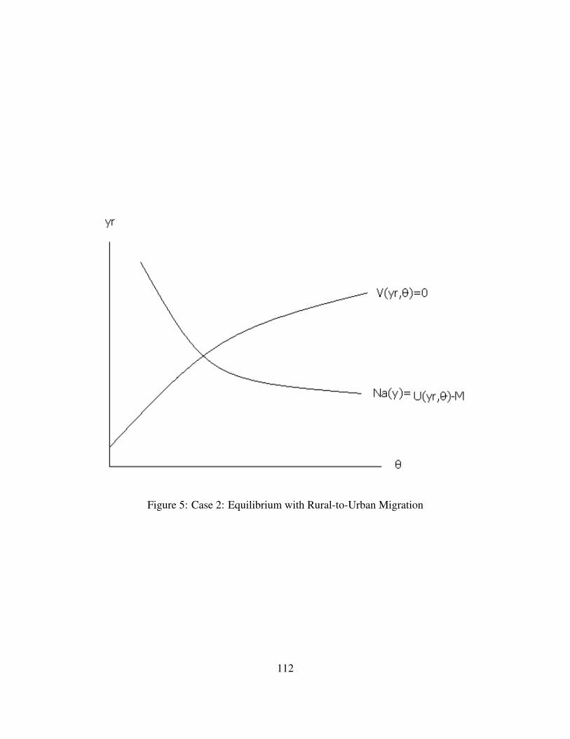
Figure 5: Case 2: Equilibrium with Rural-to-Urban Migration

112

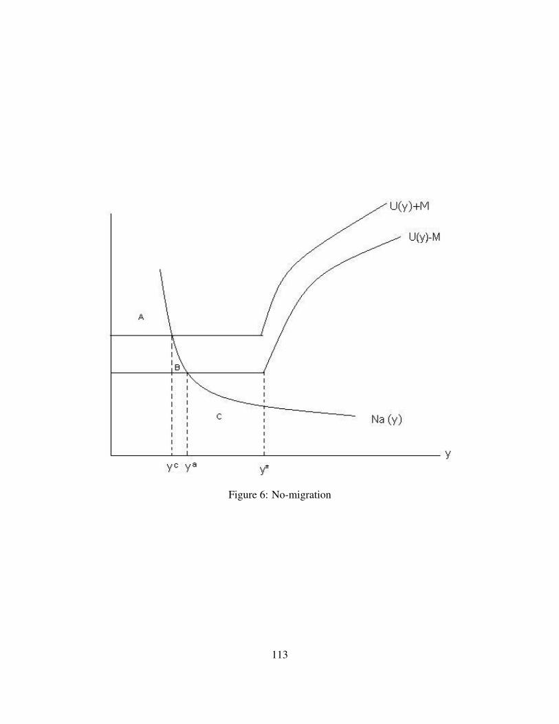
Figure 6: No-migration

113

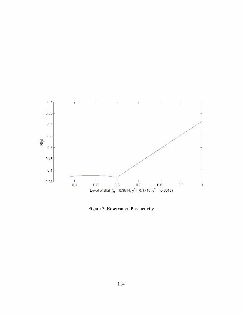
Figure 7: Reservation Productivity

114

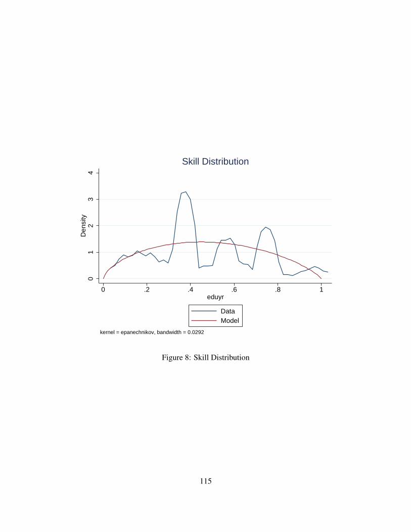
01

23

4D

ensi

ty

0 .2 .4 .6 .8 1eduyr

DataModel

kernel = epanechnikov, bandwidth = 0.0292

Skill Distribution

Figure 8: Skill Distribution

115

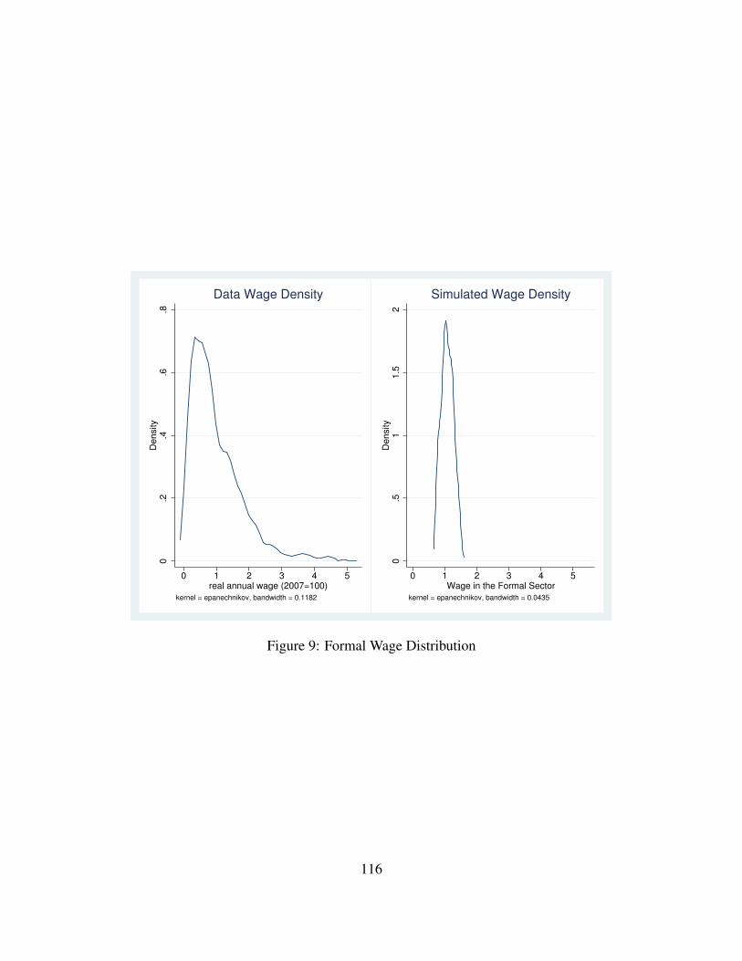
0.2

.4.6

.8D

ensity

0 1 2 3 4 5real annual wage (2007=100)

kernel = epanechnikov, bandwidth = 0.1182

Data Wage Density

0.5

11.5

2D

ensity

0 1 2 3 4 5Wage in the Formal Sector

kernel = epanechnikov, bandwidth = 0.0435

Simulated Wage Density

Figure 9: Formal Wage Distribution

116

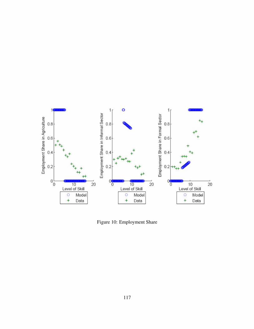
Figure 10: Employment Share

117

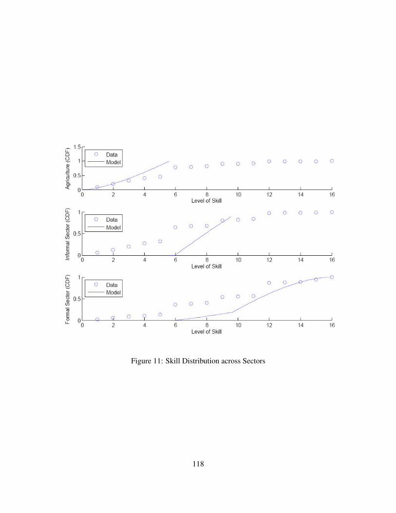
Figure 11: Skill Distribution across Sectors

118

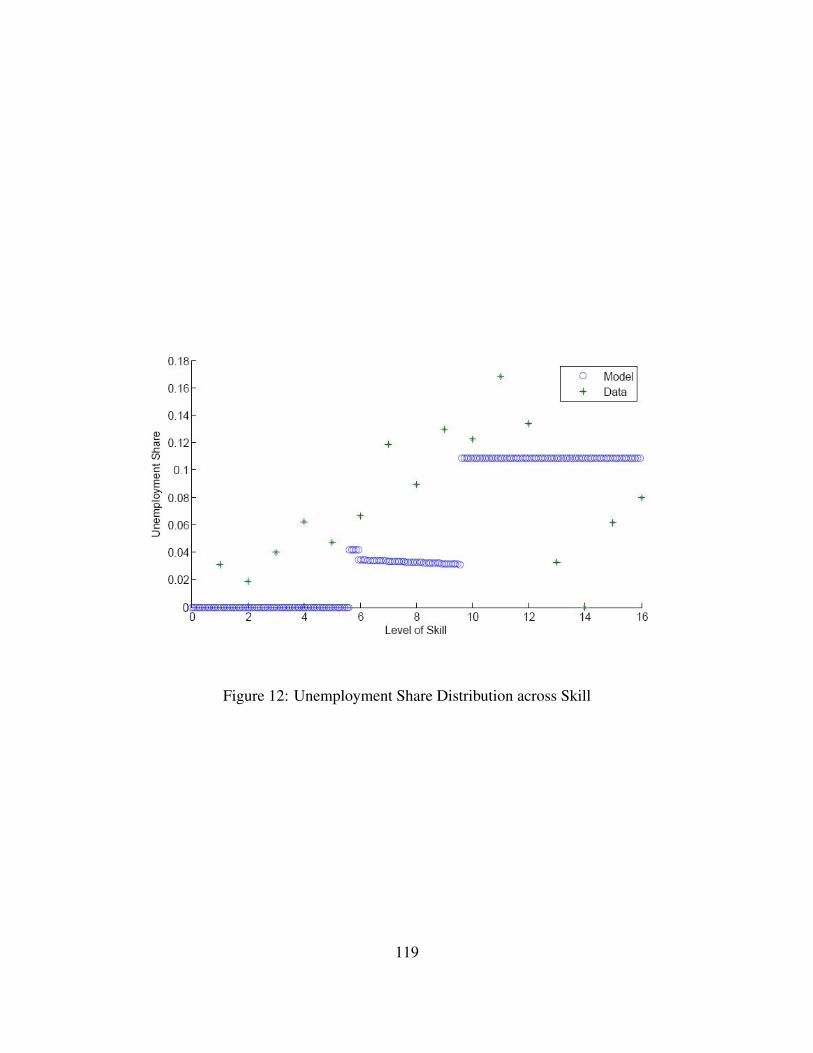
Figure 12: Unemployment Share Distribution across Skill

119

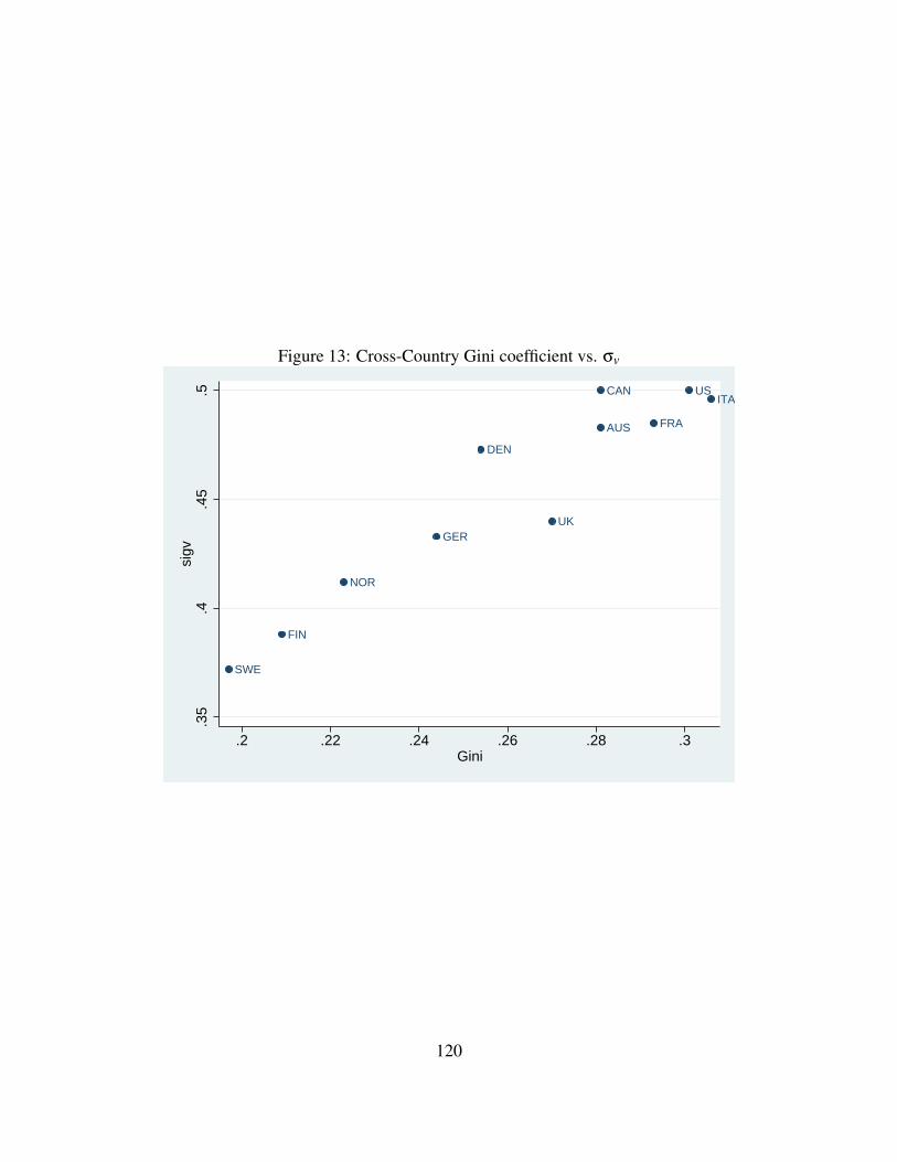
Figure 13: Cross-Country Gini coefficient vs. σv

AUS

CAN

DEN

FIN

FRA

GER

ITA

NOR

SWE

UK

US

.35

.4.4

5.5

sigv

.2 .22 .24 .26 .28 .3Gini

120

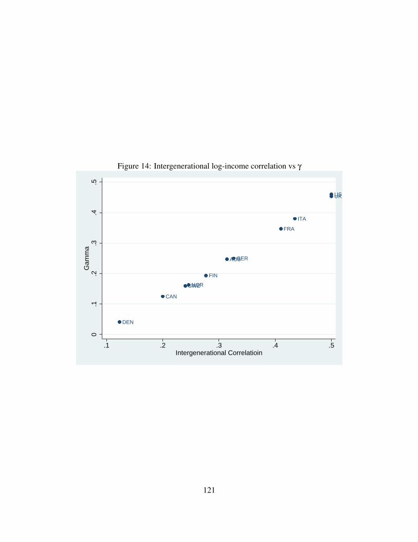
Figure 14: Intergenerational log-income correlation vs γ

AUS

CAN

DEN

FIN

FRA

GER

ITA

NORSWE

UKUS

0.1

.2.3

.4.5

Gam

ma

.1 .2 .3 .4 .5Intergenerational Correlatioin

121

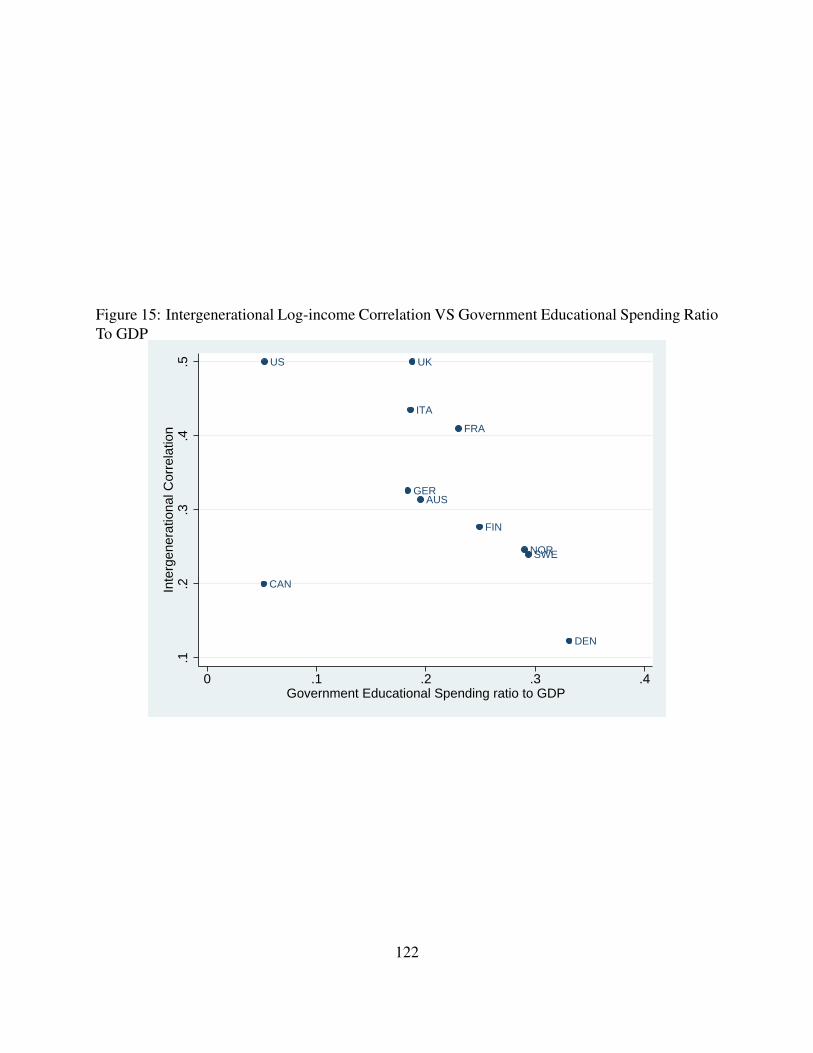
Figure 15: Intergenerational Log-income Correlation VS Government Educational Spending RatioTo GDP

AUS

CAN

DEN

FIN

FRA

GER

ITA

NORSWE

UKUS

.1.2

.3.4

.5In

terg

ener

atio

nal C

orre

latio

n

0 .1 .2 .3 .4Government Educational Spending ratio to GDP

122

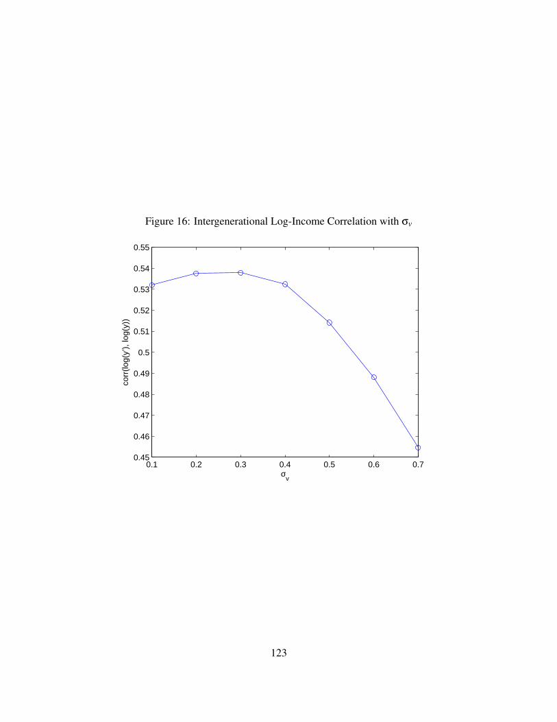
Figure 16: Intergenerational Log-Income Correlation with σv

0.1 0.2 0.3 0.4 0.5 0.6 0.70.45

0.46

0.47

0.48

0.49

0.5

0.51

0.52

0.53

0.54

0.55

σv

corr

(log(

y’),

log(

y))

123

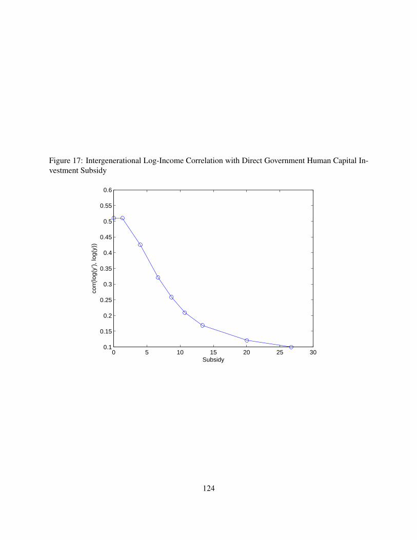
Figure 17: Intergenerational Log-Income Correlation with Direct Government Human Capital In-vestment Subsidy

0 5 10 15 20 25 300.1

0.15

0.2

0.25

0.3

0.35

0.4

0.45

0.5

0.55

0.6

Subsidy

corr

(log(

y’),

log(

y))

124

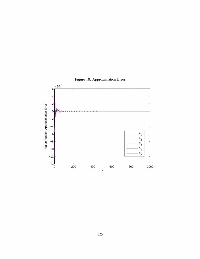
Figure 18: Approximation Error

0 200 400 600 800 1000−14

−12

−10

−8

−6

−4

−2

0

2

4

6x 10

−4

y

Val

ue F

untio

n A

ppro

xim

atio

n E

rror

a1

a2

a3

a4

a5

125