Enseñar Pensamiento Critico Ingles 1508.04870v1

Teaching critical thinking

N.G. Holmes∗

Department of Physics, Stanford University, Stanford, CA

Carl E. Wieman

Department of Physics, Stanford University, Stanford, CA and

Graduate School of Education, Stanford University, Stanford, CA

D.A. Bonn

Department of Physics and Astronomy,

University of British Columbia, Vancouver, BC

1

arX

iv:1

508.

0487

0v1

[ph

ysic

s.ed

-ph]

20

Aug

201

5

Abstract

The ability to make decisions based on data, with its inherent uncertainties and variability, is a

complex and vital skill in the modern world. The need for such quantitative critical thinking occurs

in many different contexts, and while it is an important goal of education, that goal is seldom being

achieved. We argue that the key element for developing this ability is repeated practice in making

decisions based on data, with feedback on those decisions. We demonstrate a structure for providing

suitable practice that can be applied in any instructional setting that involves the acquisition of data

and relating that data to scientific models. This study reports the results of applying that structure

in an introductory physics lab course. Students in an experimental condition were repeatedly

instructed to make and act on quantitative comparisons between datasets, and between data and

models, an approach that is common to all science disciplines. These instructions were slowly faded

across the course. After the instructions had been removed, students in the experimental condition

were 12 times more likely to spontaneously propose or make changes to improve their experimental

methods than a control group, who performed traditional experimental activities. They were also

four times more likely to identify and explain a limitation of a physical model using their data.

Students in the experimental condition also showed much more sophisticated reasoning about their

data. These differences between the groups were seen to persist into a subsequent course taken the

following year.

Significance Statement : Understanding and thinking critically about scientific evidence is a crucial

skill in the modern world. We present a simple learning framework that employs cycles of decisions

about making and acting on quantitative comparisons between datasets or data and models. With

opportunities to improve the data or models, this structure is appropriate for use in any data-driven

science learning setting. This structure led to significant and sustained improvement in students’

critical thinking behaviours, compared to a control group, with effects far beyond that of statistical

significance.

Keywords: critical thinking — scientific reasoning — scientific teaching — teaching experimentation

— undergraduate education

Published in the Proceedings of the National Academy of Sciences.doi:10.1073/pnas.1505329112

2

A central goal of science education is to teach students to think critically about scientific

data and models. It is crucial for scientists, engineers, and citizens in all walks of life to

be able to critique data, to identify whether or not conclusions are supported by evidence,

and to distinguish a significant effect from random noise and variability. There are many

indications of how difficult it is for people to master this type of thinking as evidenced by

many societal debates. Although teaching quantitative critical thinking is a fundamental

goal of science education, particularly the laboratory portion, the evidence indicates this is

seldom, if ever, being achieved [1–6]. To address this educational need, we have analyzed

the explicit cognitive processes involved in such critical thinking and then developed an

instructional design to incorporate these processes.

We argue that scientists engage in such critical thinking through a process of repeated

comparisons and decisions: comparing new data to existing data and/or models, and then

deciding how to act on those comparisons based on analysis tools that embody appropriate

statistical tests. Those actions typically lead to further iterations involving improving the

data and/or modifying the experiment or model. In a research setting, common decisions

are to improve the quality of measurements (in terms of accuracy or precision) to determine

whether an effect is hidden by large variability, to embrace, adjust or discard a model based

on the scientific evidence, or to devise a new experiment to answer the question. In other

settings, such as medical policy decisions, there may be fewer options but corresponding

decisions are made as to the consistency of the model and the data and what conclusions

are justified by the data.

We hypothesize that much of the reason students do not engage in these behaviours is

because the educational environment provides few opportunities for this process. Students

ought to be explicitly exposed to how experts engage in critical thinking in each specific

discipline, which should, in turn, expose them to the nature of knowledge in that discipline

[7]. Demonstrating the critical thinking process, of course, is insufficient for students to use

it on their own. Students need practice engaging in the critical thinking process themselves,

and this practice should be deliberate and repeated with targeted feedback [7–9]. We do

not expect first year university students to engage in expert-level thinking processes. We

∗ [email protected]


3

can train them to think more like scientists by simplifying the expert decision tree described

above. Making it explicit to students, demonstrating how it allows them to learn or make

discoveries, and having them practice in a deliberate way with targeted feedback, will help

students understand the nature of scientific measurement and data uncertainty, and, in time,

adopt the new ways of thinking.

The decision tree and iterative process we have described could be provided in any setting

in which data and models are introduced to students. Virtually all instructional labs in

science offer such opportunities as students collect data and use it to explore various models

and systems. Such labs are an ideal environment for developing students’ critical thinking

and this is arguably their greatest value beyond simply skills-training.

We have tested this instructional concept in the context of a calculus-based introductory

laboratory course in physics at a research-intensive university. The students repeatedly and

explicitly make decisions and act on comparisons between data sets or between data and

models as they work through a series of simple, introductory physics experiments. Although

this study is in the context of a physics course, we believe the effect would be similar using

experiments from any subject that involve quantitative data, opportunities to quantitatively

compare data and models, and opportunities to improve data and models. With this simple

intervention, we observed dramatic long-term improvements in students’ quantitative critical

thinking behaviours when compared with a control group that carried out the same lab

experiments, but with a structure more typical of instructional labs.

In our study, students in the experiment condition were explicitly instructed to (and

received grades to) quantitatively compare multiple collected data sets or a collected data

set and a model, and to decide how to act on the comparisons (figure 1). While a variety

of options for acting on comparisons, as listed above, were presented to students, striving to

improve the quality of their data was the most rigorously enforced. For example, in one of

the earliest experiments, students were told to make two sets of measurements and compare

them quantitatively. They were then prompted to devise a plan to improve the quality of

their measurements, to discuss this plan with other groups, and to carry out the revised

measurements and analysis. This explicit focus on measurements, rather than improving

models, was intended to address the fact that students in a lab course often assume data


4

they collect is inherently low quality compared to expert results [10]. This can lead them to

ignore disagreements between measurements or to artificially inflate uncertainties to disguise

them [11]. When disagreements do arise, students often attribute them to what they refer

to as ‘human error’ [12] or simply blame the equipment being used. As such, students are

unlikely to adjust or discard an authoritative model, since they do not trust that their data is

sufficiently high quality to make such a claim. We hypothesize that the focus on high-quality

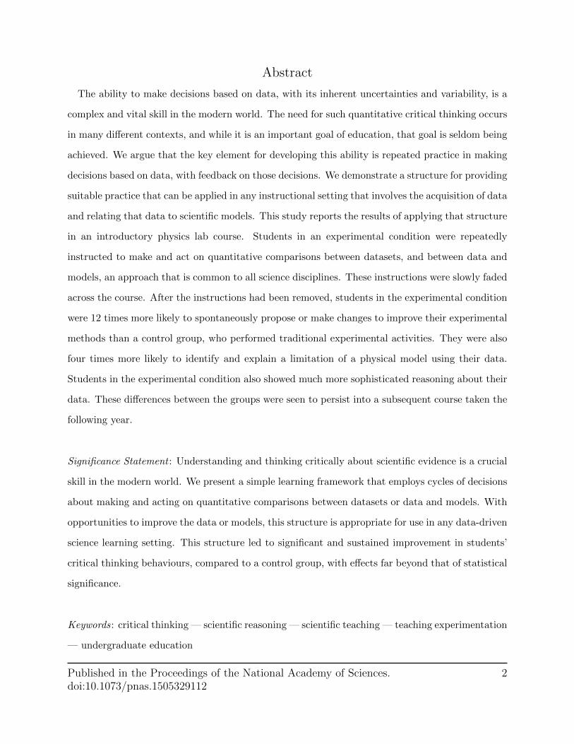
data will, over time, encourage students to critique models without explicit support.Scaffold(the(cri.cal(thinking(

14

Make a Comparison

Act on the comparison

Reflect on Comparison

FIG. 1: The experimental condition engaged students in iterative cycles of making andacting on comparisons of their data. This involved comparing pairs of measurements with

uncertainty or comparing data sets to models using weighted χ2 and residual plots.

To compare measurements quantitatively, students were taught a number of analysis tools

used regularly by scientists in any field. Students were also taught a framework for how to

use these tools to make decisions about how to act on the comparisons. For example, they

were shown weighted χ2 calculations for least squares fitting of data to models and then were

given a decision tree for interpreting the outcome. If they obtain a low χ2 they would decide

whether it means their data is in good agreement with the model or whether it means they

have overestimated their uncertainties. If they obtain a large χ2 they would decide whether

there is an issue with the model or with the data. From these interpretations, the decision

tree expands into deciding what to do. In both cases, students were encouraged to improve

their data: to improve precision and decrease their uncertainties in the case of low χ2, or

to identify measurement or systematic errors in the case of a large χ2. While they were

told that a large χ2 might reflect an issue with the model, they were not told what to do

about it, leaving room for autonomous decision making. Regardless of the outcome of the


5

comparison, therefore, students had guidelines for how to act on the comparison, typically

leading to additional measurements. This naturally led to iterative cycles of making and

acting on comparisons, which could be used for any type of comparison.

Before working with χ2 fitting and models, students were first introduced to an index for

comparing pairs of measured values with uncertainty (the ratio of the difference between two

measured values to the uncertainty in the difference, see S1.1 for more details). Students

were also taught to plot residuals (the point-by-point difference between measured data

and a model) to visualize the comparison of data and models. Both of these tools, and

any comparison tool that includes the variability in a measurement, lend themselves to

the same decision process as the χ2 value when identifying disagreements with models or

improving data quality. A number of standard procedural tools for determining uncertainty

in measurements or fit parameters were also taught (see S1.1 for the full list). As more

tools were introduced during the course, the explicit instructions to make or act on the

comparisons were faded (see S1.2 for more details and for a week-by-week diagram of the

fading).

The students carried out different experiments each week and completed the analysis

within the three-hour lab period. To evaluate the impact of the comparison cycles, we

assessed students’ written lab work from three lab sessions (see S1.3 for a description of the

experiments) from the course: one early in the course when the experimental group had

explicit instructions to perform comparison cycles to improve data (week 2), and two when

all instruction about making and acting on comparisons had been stopped (weeks 16 and

17). We also examined student work from a quite different lab course taken by the same

students in the following year. About a third of the students from the first-year lab course

progressed into the second year (sophomore) physics lab course. This course had different

instructors, experiments, and structure. Students carried out a smaller number of more

complex experiments, each one completed over two weeks, with final reports then submitted

electronically. We analyzed the student work on the third experiment in this course.


6

RESULTS

Students’ written work was evaluated for evidence of acting on comparisons, either sug-

gesting or executing changes to measurement procedures, or critiquing or modifying physical

models in light of collected data. We also examined students’ reasoning about data to fur-

ther inform the results (see S1.4 for inter-rater reliability of the coding process for these

three measures). Student performance in the experimental group (n ≈ 130) was compared

with a control group (n ≈ 130). The control was a group of students who had taken the

course the previous year with the same set of experiments. Analysis in the supplementary

material demonstrates that the groups were equivalent in performance on conceptual physics

diagnostic tests (S1.5). Although both groups were taught similar data analysis methods

(such as weighted χ2 fitting), the control group was neither instructed nor graded on making

or acting on cycles of quantitative comparisons. They also were not introduced to plotting

residuals or comparing differences of pairs of measurements as a ratio of the combined un-

certainty. However, instructions given to the experimental group were faded over time, so

the instructions given to both groups were identical in week 16 and week 17.

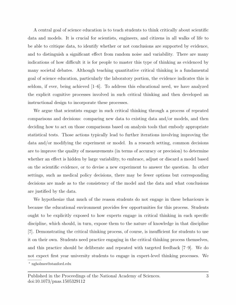
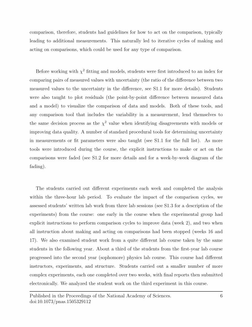
We first compiled all instances where students decided to act on comparisons by propos-

ing and/or making changes to their methods (figure 2), since this was the most explicitly

structured behaviour for the experimental group. When students in the experimental group

were instructed to iterate and improve their measurements (week 2), nearly all students

proposed or carried out such changes. By the end of the course, when the instructions had

been removed, over half of the experimental group continued to make or propose changes to

their data or methods. This fraction was similar for the sophomore lab experiment, where

it was evident that they were making changes, even though we were evaluating final reports

rather than laboratory notebooks. Almost none of the control group did at any time.

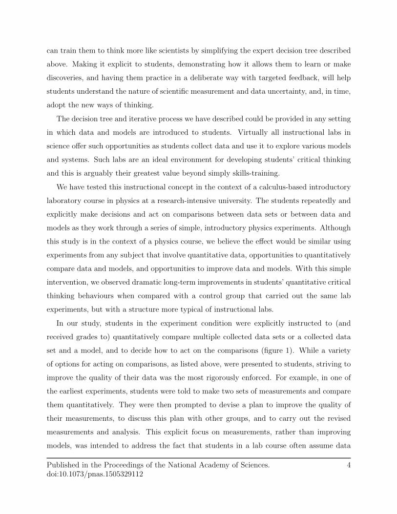
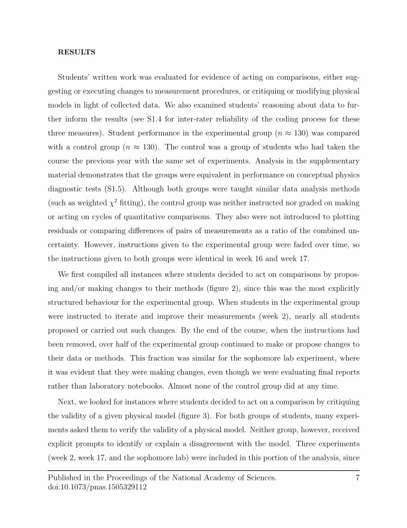
Next, we looked for instances where students decided to act on a comparison by critiquing

the validity of a given physical model (figure 3). For both groups of students, many experi-

ments asked them to verify the validity of a physical model. Neither group, however, received

explicit prompts to identify or explain a disagreement with the model. Three experiments

(week 2, week 17, and the sophomore lab) were included in this portion of the analysis, since


7

Week 2 Week 16 Week 17

0.00

0.25

0.50

0.75

1.00

Control Experiment Control Experiment Control ExperimentFirst Year Lab

Fra

ctio

n of

Stu

dent

sSophomore Lab

Control ExperimentSophomore Lab

Proposed only

Proposed & Changed

FIG. 2: Method Changes. The fraction of students proposing and/or carrying outchanges to their experimental methods over time shows a large and sustained difference

between the experimental and control groups. This difference is substantial when studentsin the experimental group were prompted to make changes (Week 2), but continues evenwhen instructions to act on the comparisons are removed (Week 16 and 17). This evenoccurs into the sophomore lab course (see S2.1 for statistical analyses). Note that the

sophomore lab data represents a fraction ( 1/3) of the first year lab population.Uncertainty bars represent 67% confidence intervals on the total proportions of students

proposing or carrying out changes in each group each week.

these experiments involved physical models that were limited or insufficient for the quality

of data achievable (see S1.3). In all three experiments, students’ written work was coded for

whether they identified a disagreement between their data and the model and whether they

correctly interpreted the disagreement in terms of the limitations of the model.

As shown in figure 3, few students in either group noted a disagreement in week 2. As

previously observed, learners tend to defer to authoritative information [7, 10, 11]. In fact,

many students in the experimental group stated that they wanted to improve their data to

get better agreement, ignoring the possibility that there could be something wrong with the


8

Week 2 Week 17

0.00

0.25

0.50

0.75

1.00

Control Experiment Control ExperimentFirst Year Lab

Fra

ctio

n of

Stu

dent

sSophomore Lab

Control ExperimentSophomore Lab

Identified

Identified & Interpreted

FIG. 3: Evaluating Models. The fraction of students that identified and correctlyinterpreted disagreements between their data and a physical model shows significant gainsby the experiment group across the lab course (see S2.2 for statistical analyses). This effectis sustained into the sophomore lab. Note that the sophomore lab students were prompted

about an issue with the model, which explains the increase in the number of studentsidentifying the issue in the control group. Uncertainty bars represent 67% confidence

intervals on the total proportions of students identifying or interpreting the modeldisagreements in each group each week.

model.

As they progress in the course, however, dramatic changes emerge. In week 17, over

3/4 of the students in the experimental group identified the disagreement, nearly four times

more than in the control group, and over half of the experimental group provided the correct

physical interpretation. Students in the experimental group showed similar performance in

the sophomore lab, indicating that the quantitative critical thinking was carried forward.

The lab instructions for the sophomore experiment provided students with a hint that a

technical modification to the model equation may be necessary if the fit was unsatisfactory,


9

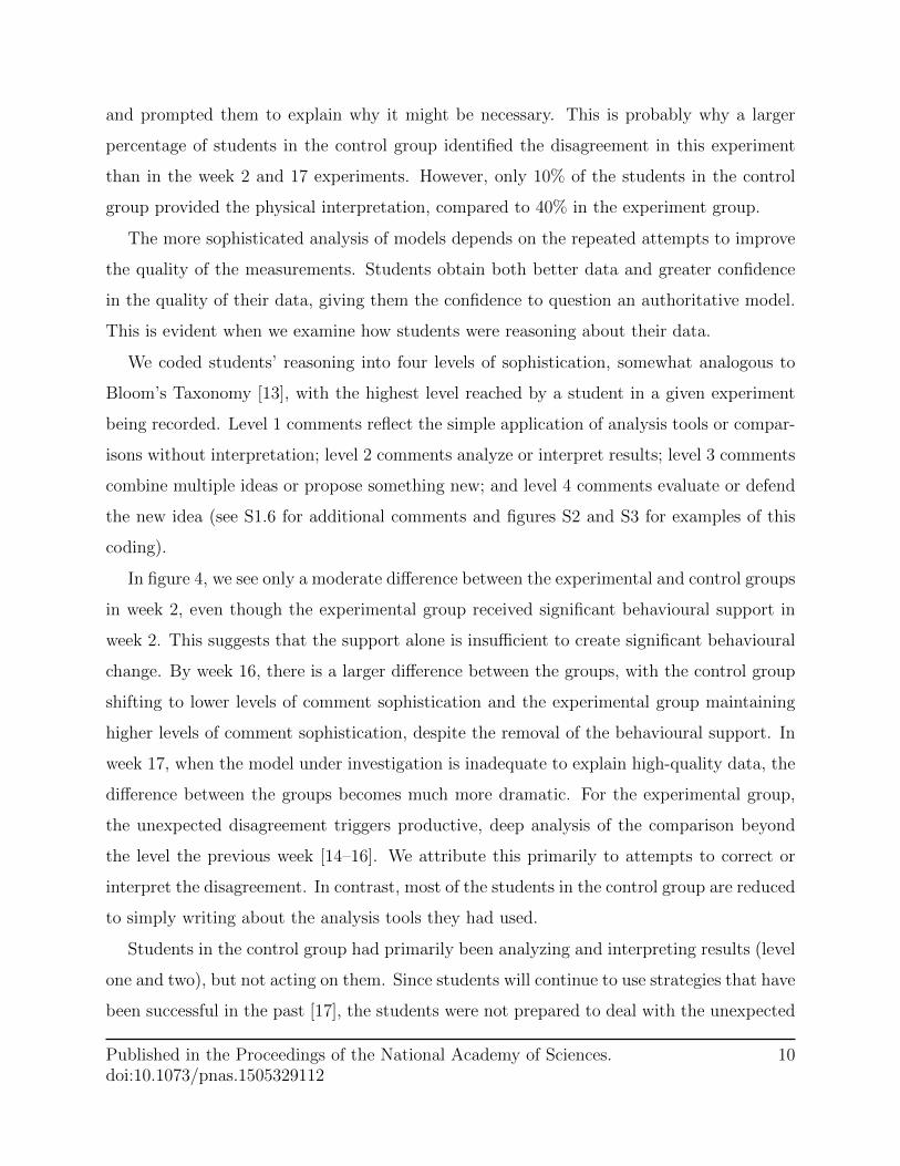
and prompted them to explain why it might be necessary. This is probably why a larger

percentage of students in the control group identified the disagreement in this experiment

than in the week 2 and 17 experiments. However, only 10% of the students in the control

group provided the physical interpretation, compared to 40% in the experiment group.

The more sophisticated analysis of models depends on the repeated attempts to improve

the quality of the measurements. Students obtain both better data and greater confidence

in the quality of their data, giving them the confidence to question an authoritative model.

This is evident when we examine how students were reasoning about their data.

We coded students’ reasoning into four levels of sophistication, somewhat analogous to

Bloom’s Taxonomy [13], with the highest level reached by a student in a given experiment

being recorded. Level 1 comments reflect the simple application of analysis tools or compar-

isons without interpretation; level 2 comments analyze or interpret results; level 3 comments

combine multiple ideas or propose something new; and level 4 comments evaluate or defend

the new idea (see S1.6 for additional comments and figures S2 and S3 for examples of this

coding).

In figure 4, we see only a moderate difference between the experimental and control groups

in week 2, even though the experimental group received significant behavioural support in

week 2. This suggests that the support alone is insufficient to create significant behavioural

change. By week 16, there is a larger difference between the groups, with the control group

shifting to lower levels of comment sophistication and the experimental group maintaining

higher levels of comment sophistication, despite the removal of the behavioural support. In

week 17, when the model under investigation is inadequate to explain high-quality data, the

difference between the groups becomes much more dramatic. For the experimental group,

the unexpected disagreement triggers productive, deep analysis of the comparison beyond

the level the previous week [14–16]. We attribute this primarily to attempts to correct or

interpret the disagreement. In contrast, most of the students in the control group are reduced

to simply writing about the analysis tools they had used.

Students in the control group had primarily been analyzing and interpreting results (level

one and two), but not acting on them. Since students will continue to use strategies that have

been successful in the past [17], the students were not prepared to deal with the unexpected


10

First Year − Control First Year − Experiment

0.0

0.5

1.0

0.0

0.5

1.0

0.0

0.5

1.0

Week 2

Week 16

Week 17

Fra

ctio

n of

stu

dent

s

Sophomore Lab − Control Sophomore Lab − Experiment

0.0

0.5

1.0

1 2 3 4 1 2 3 4Maximum Reflective Comment Level

FIG. 4: Reflective comments. The distribution of the maximum reflection commentlevel students reached in four different experiments (three in the first year course and one

in the sophomore course) shows statistically significant differences between groups (see S2.3for statistical analyses). Uncertainty bars represent 67% confidence intervals on the

proportions of students.

outcome in week 17. Our data, however, is limited in that we only evaluate what was written

in their books by the end of the lab session. It is plausible that the students in the control

group were holding high-level discussions about the disagreement, but not writing them

down. Their low-level written reflections are, at best, evidence that they needed more time

to achieve the outcomes of the experiment group.

In the sophomore lab, the students in the experimental group continued to show a high

level in their reflective comments, showing a sustained change in reasoning and epistemology.

The students in the control group show higher-level reflections in the sophomore lab than

they did in the first-year lab, possibly because of the greater time given to analyze their

data, the prompt about the model failing, or the selection of these students as physics

majors. They still remained well below the level of the experimental group, nonetheless.


11

DISCUSSION

The cycles of making and deciding how to act on quantitative comparisons gave students

experience with making authentic scientific decisions about data and models. Since students

had to ultimately decide how to proceed, the cycles provided a constrained experimental

design space to prepare them for autonomous decision-making [18]. With a focus on the

quality of their data and how they could improve it, they came to believe that they are able

to test and evaluate models. This is not just an acquisition of skills; it is an attitudinal

and epistemological shift unseen in the control group or in other studies of instructional labs

[11, 12]. The training in how to think like an expert inherently teaches students how experts

think and, thus, how experts generate knowledge [7].

The simple nature of the structure employed here gives students both a framework and

a habit of mind that leaves them better prepared to transfer the skills and behaviours to

new contexts [19–21]. This simplicity also makes it easily generalizable to a very wide range

of instructional settings; any venue that contains opportunities to make decisions based on

comparisons.

ACKNOWLEDGMENTS

The authors would like to acknowledge the support of Deborah Butler in preparing the

manuscript. We would also like to thank Jim Carolan for the diagnostic survey data about the

study participants. This research was supported by UBC’s Carl Wieman Science Education

Initiative.

[1] Kanari Z and Millar R (2004) Reasoning from data: How students collect and interpret data

in science investigations. J Res Sci Teach 41(7):748-769.

[2] Kumassah E-K, Ampiah J-G, and Adjei E-J (2013) An investigation into senior high school

(shs3) physics students understanding of data processing of length and time of scientific mea-


12

surement in the Volta region of Ghana. International Journal of Research Studies in Educa-

tional Technology 3(1):37-61.

[3] Kung R-L and Linder C (2006) University students’ ideas about data processing and data

comparison in a physics laboratory course. Nordic Studies in Science Education 2(2):40-53.

[4] Ryder J and Leach J (2000) Interpreting experimental data: the views of upper secondary

school and university science students. Int J Sci Educ 22(10):1069-1084.

[5] Ryder J (2002) Data Interpretation Activities and Students’ Views of the Epistemology of

Science during a University Earth Sciences Field Study Course. Teaching and Learning in the

Science Laboratory, eds. Psillos D, Niedderer H(Springer Netherlands), pp 151-162.

[6] Sere M-G, Journeaux R, and Larcher C (1993) Learning the statistical analysis of measurement

errors. Int J Sci Educ 15(4):427-438.

[7] Baron J (1993) Why Teach Thinking? - An Essay. Appl Psych 42(3):191-214.

[8] Ericsson K-A, Krampe R-T, and Tesch-Romer C (1993) The role of deliberate practice in the

acquisition of expert performance. Psychol Rev 100(3):363-406.

[9] Kuhn D and Pease M (2008) What Needs to Develop in the Development of Inquiry Skills?

Cognition Instruct 26(4):512-559.

[10] Allie S, Buffler A, Campbell B, and Lubben F (1998) First-year physics students’ perceptions

of the quality of experimental measurements. Int J Sci Educ 20(4):447-459.

[11] Holmes N-G and Bonn D-A (2013) Doing Science Or Doing A Lab? Engaging Students

With Scientific Reasoning During Physics Lab Experiments. 2013 PERC Proceedings, eds.

Engelhardt P-V, Churukian A-D, and Jones D-L (Portland, OR):185-188.

[12] Sere M-G, Fernandez-Gonzalez M, Gallegos J-A, Gonzalez-Garcia F, De Manuel E, Perales

F-J, and Leach J (2001) Images of Science Linked to Labwork: A Survey of Secondary School

and University Students Res Sci Educ 31(4):499-523.

[13] Anderson L-W and Sosniak L-A (1994) Bloom’s taxonomy: A forty-year retrospective (NSSE:

University of Chicago Press, Chicago, IL).

[14] Holmes N-G, Ives J, and Bonn D-A (2014) The Impact of Targeting Scientific Reasoning on

Student Attitudes about Experimental Physics. 2014 PERC Proceedings, eds. Engelhardt P-V,

Churukian A-D, and Jones D-L (Minneapolis, MN).


13

[15] Kapur M (2008) Productive Failure. Cognition Instruct 26(3):379-424.

[16] VanLehn K (1988) Toward a Theory of Impasse-Driven Learning. Cognitive Sci, eds. Mandl

H and Lesgold A (Springer, US) pp. 19-41.

[17] Butler, D-L (2002) Individualizing Instruction in Self-Regulated Learning. Theor Pract

41(2):81-92.

[18] Sere M-G (2002) Towards renewed research questions from the outcomes of the European

project Labwork in Science Education. Sci Educ 86(5):624-644.

[19] Bulu S and Pedersen S (2010) Scaffolding middle school students’ content knowledge and

ill-structured problem solving in a problem-based hypermedia learning environment. ETR&D-

Educ Tech Res 58(5):507-529.

[20] Salomon G and Perkins D-N (1989) Rocky Roads to Transfer: Rethinking Mechanism of a

Neglected Phenomenon. Educ Psychol 24(2):113-142.

[21] Sternberg R-J and Ben-Zeev T (2001) Complex cognition: The psychology of human thought

(Oxford University Press).

[22] Krzywinski M and Altman N (2013) Points of Significance: Error bars. Nat Methods

10(10):921-922.

[23] BIPM, IEC, IFCC, ISO, IUPAC, IUPAP, and OIML (2008) Guides to the expression of un-

certainty in measurement (Organization for Standardization).

[24] Ding L, Chabay R, Sherwood B, and Beichner R (2006) Evaluating an electricity and mag-

netism assessment tool: Brief electricity and magnetism assessment. Phys Rev Spec Top-PH

2(1):010105

[25] Hestenes D and Wells M (1992) A mechanics baseline test. Phys Teach 30(3):159-.

[26] Hestenes D, Wells M, and Swackhamer G (1992) Force concept inventory. Phys Teach

30(3):141-158.

[27] R Core Team (2014) R: A language and environment for statistical computing. (R Foundation

for Statistical Computing).

[28] Bates D, Maechler M, Bolker B, and Walker S (2014) lme4: Linear mixed-effects models using

Eigen and S4. (R Foundation for Statistical Computing).


14

[29] Fox J and Weisberg S (2011) An R Companion to Applied Regression. R Foundation for

Statistical Computing.

[30] Hofstein A and Lunetta V-N (2004) The laboratory in science education: Foundations for the

twenty-first century. Sci Educ 88(1):28-54.


15

Teaching critical thinking

N.G. Holmes∗

Department of Physics, Stanford University, Stanford, CA

Carl E. Wieman

Department of Physics, Stanford University, Stanford, CA and

Graduate School of Education, Stanford University, Stanford, CA

D.A. Bonn

Department of Physics and Astronomy,

University of British Columbia, Vancouver, BC

1

arX

iv:1

508.

0487

0v1

[ph

ysic

s.ed

-ph]

20

Aug

201

5

SUPPLEMENTARY MATERIALS

S1. QUANTITATIVE COMPARISON TOOLS

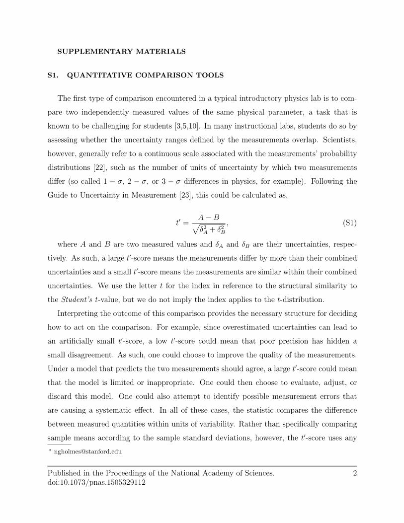
The first type of comparison encountered in a typical introductory physics lab is to com-

pare two independently measured values of the same physical parameter, a task that is

known to be challenging for students [3,5,10]. In many instructional labs, students do so by

assessing whether the uncertainty ranges defined by the measurements overlap. Scientists,

however, generally refer to a continuous scale associated with the measurements’ probability

distributions [22], such as the number of units of uncertainty by which two measurements

differ (so called 1 − σ, 2 − σ, or 3 − σ differences in physics, for example). Following the

Guide to Uncertainty in Measurement [23], this could be calculated as,

t′ =A−B√δ2A + δ2B

, (S1)

where A and B are two measured values and δA and δB are their uncertainties, respec-

tively. As such, a large t′-score means the measurements differ by more than their combined

uncertainties and a small t′-score means the measurements are similar within their combined

uncertainties. We use the letter t for the index in reference to the structural similarity to

the Student’s t-value, but we do not imply the index applies to the t-distribution.

Interpreting the outcome of this comparison provides the necessary structure for deciding

how to act on the comparison. For example, since overestimated uncertainties can lead to

an artificially small t′-score, a low t′-score could mean that poor precision has hidden a

small disagreement. As such, one could choose to improve the quality of the measurements.

Under a model that predicts the two measurements should agree, a large t′-score could mean

that the model is limited or inappropriate. One could then choose to evaluate, adjust, or

discard this model. One could also attempt to identify possible measurement errors that

are causing a systematic effect. In all of these cases, the statistic compares the difference

between measured quantities within units of variability. Rather than specifically comparing

sample means according to the sample standard deviations, however, the t′-score uses any

∗ [email protected]


2

measurement value with its uncertainty. As such, we do not try to compare the t′-scores on

the t-distribution or make inferences about probabilities. Indeed, if the measurements were

sample means from populations with the same variance, the t′-score would be equivalent to

Student’s t for comparing independent samples (or, if homogeneity of variance is violated,

the t′-score would be equivalent to Welch’s t).

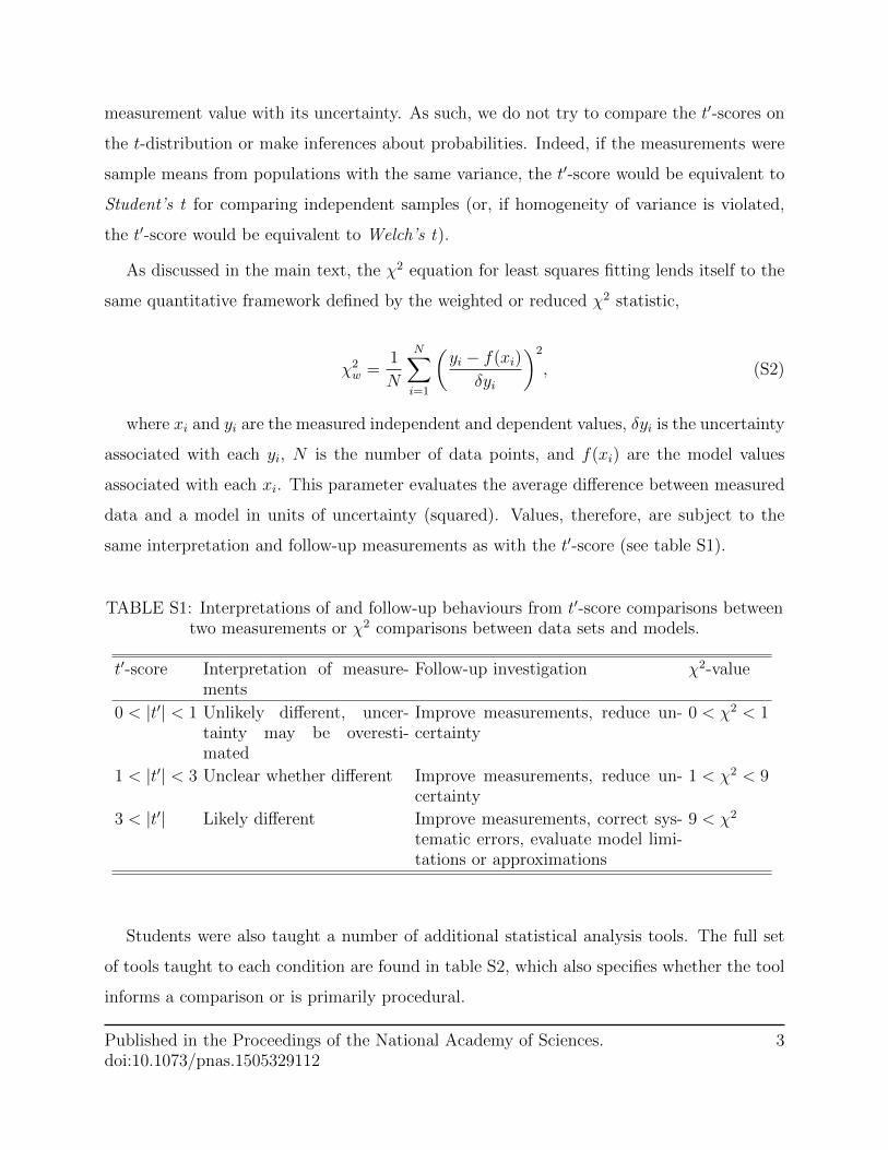
As discussed in the main text, the χ2 equation for least squares fitting lends itself to the

same quantitative framework defined by the weighted or reduced χ2 statistic,

χ2w =

1

N

N∑

i=1

(yi − f(xi)

δyi

)2

, (S2)

where xi and yi are the measured independent and dependent values, δyi is the uncertainty

associated with each yi, N is the number of data points, and f(xi) are the model values

associated with each xi. This parameter evaluates the average difference between measured

data and a model in units of uncertainty (squared). Values, therefore, are subject to the

same interpretation and follow-up measurements as with the t′-score (see table S1).

TABLE S1: Interpretations of and follow-up behaviours from t′-score comparisons betweentwo measurements or χ2 comparisons between data sets and models.

t′-score Interpretation of measure-ments

Follow-up investigation χ2-value

0 < |t′| < 1 Unlikely different, uncer-tainty may be overesti-mated

Improve measurements, reduce un-certainty

0 < χ2 < 1

1 < |t′| < 3 Unclear whether different Improve measurements, reduce un-certainty

1 < χ2 < 9

3 < |t′| Likely different Improve measurements, correct sys-tematic errors, evaluate model limi-tations or approximations

9 < χ2

Students were also taught a number of additional statistical analysis tools. The full set

of tools taught to each condition are found in table S2, which also specifies whether the tool

informs a comparison or is primarily procedural.


3

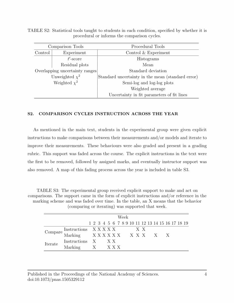
TABLE S2: Statistical tools taught to students in each condition, specified by whether it isprocedural or informs the comparison cycles.

Comparison Tools Procedural Tools

Control Experiment Control & Experiment

t′-score Histograms

Residual plots Mean

Overlapping uncertainty ranges Standard deviation

Unweighted χ2 Standard uncertainty in the mean (standard error)

Weighted χ2 Semi-log and log-log plots

Weighted average

Uncertainty in fit parameters of fit lines

S2. COMPARISON CYCLES INSTRUCTION ACROSS THE YEAR

As mentioned in the main text, students in the experimental group were given explicit

instructions to make comparisons between their measurements and/or models and iterate to

improve their measurements. These behaviours were also graded and present in a grading

rubric. This support was faded across the course. The explicit instructions in the text were

the first to be removed, followed by assigned marks, and eventually instructor support was

also removed. A map of this fading process across the year is included in table S3.

TABLE S3: The experimental group received explicit support to make and act oncomparisons. The support came in the form of explicit instructions and/or reference in the

marking scheme and was faded over time. In the table, an X means that the behavior(comparing or iterating) was supported that week.

Week

1 2 3 4 5 6 7 8 9 10 11 12 13 14 15 16 17 18 19

CompareInstructions X X X X X X X

Marking X X X X X X X X X X X

IterateInstructions X X X

Marking X X X X


4

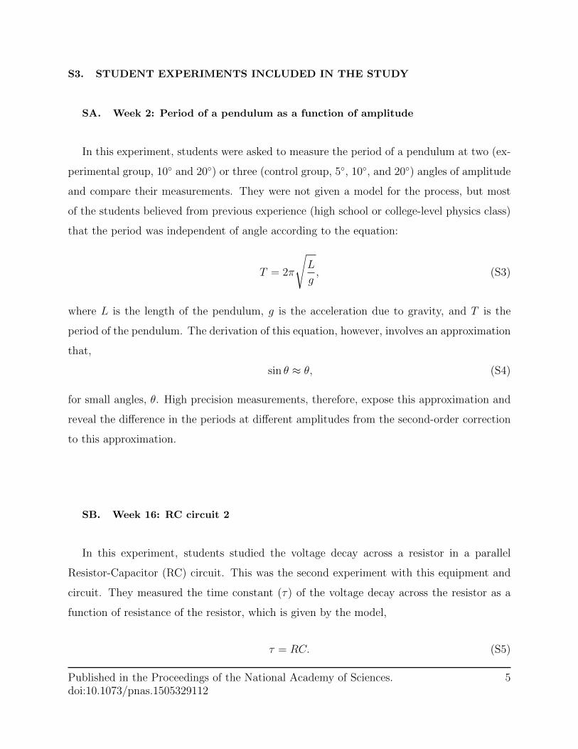
S3. STUDENT EXPERIMENTS INCLUDED IN THE STUDY

SA. Week 2: Period of a pendulum as a function of amplitude

In this experiment, students were asked to measure the period of a pendulum at two (ex-

perimental group, 10◦ and 20◦) or three (control group, 5◦, 10◦, and 20◦) angles of amplitude

and compare their measurements. They were not given a model for the process, but most

of the students believed from previous experience (high school or college-level physics class)

that the period was independent of angle according to the equation:

T = 2π

√L

g, (S3)

where L is the length of the pendulum, g is the acceleration due to gravity, and T is the

period of the pendulum. The derivation of this equation, however, involves an approximation

that,

sin θ ≈ θ, (S4)

for small angles, θ. High precision measurements, therefore, expose this approximation and

reveal the difference in the periods at different amplitudes from the second-order correction

to this approximation.

SB. Week 16: RC circuit 2

In this experiment, students studied the voltage decay across a resistor in a parallel

Resistor-Capacitor (RC) circuit. This was the second experiment with this equipment and

circuit. They measured the time constant (τ) of the voltage decay across the resistor as a

function of resistance of the resistor, which is given by the model,

τ = RC. (S5)


5

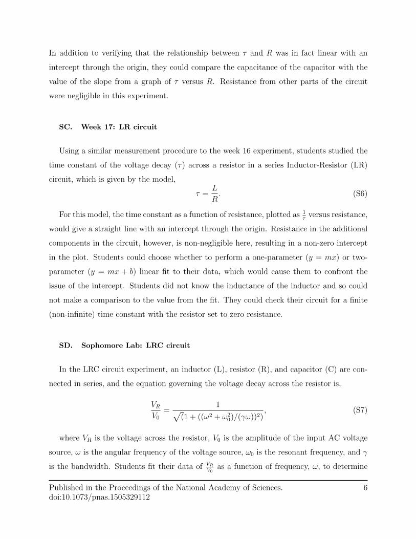
In addition to verifying that the relationship between τ and R was in fact linear with an

intercept through the origin, they could compare the capacitance of the capacitor with the

value of the slope from a graph of τ versus R. Resistance from other parts of the circuit

were negligible in this experiment.

SC. Week 17: LR circuit

Using a similar measurement procedure to the week 16 experiment, students studied the

time constant of the voltage decay (τ) across a resistor in a series Inductor-Resistor (LR)

circuit, which is given by the model,

τ =L

R. (S6)

For this model, the time constant as a function of resistance, plotted as 1τ

versus resistance,

would give a straight line with an intercept through the origin. Resistance in the additional

components in the circuit, however, is non-negligible here, resulting in a non-zero intercept

in the plot. Students could choose whether to perform a one-parameter (y = mx) or two-

parameter (y = mx + b) linear fit to their data, which would cause them to confront the

issue of the intercept. Students did not know the inductance of the inductor and so could

not make a comparison to the value from the fit. They could check their circuit for a finite

(non-infinite) time constant with the resistor set to zero resistance.

SD. Sophomore Lab: LRC circuit

In the LRC circuit experiment, an inductor (L), resistor (R), and capacitor (C) are con-

nected in series, and the equation governing the voltage decay across the resistor is,

VRV0

=1√

(1 + ((ω2 + ω20)/(γω))2)

, (S7)

where VR is the voltage across the resistor, V0 is the amplitude of the input AC voltage

source, ω is the angular frequency of the voltage source, ω0 is the resonant frequency, and γ

is the bandwidth. Students fit their data of VRV0

as a function of frequency, ω, to determine


6

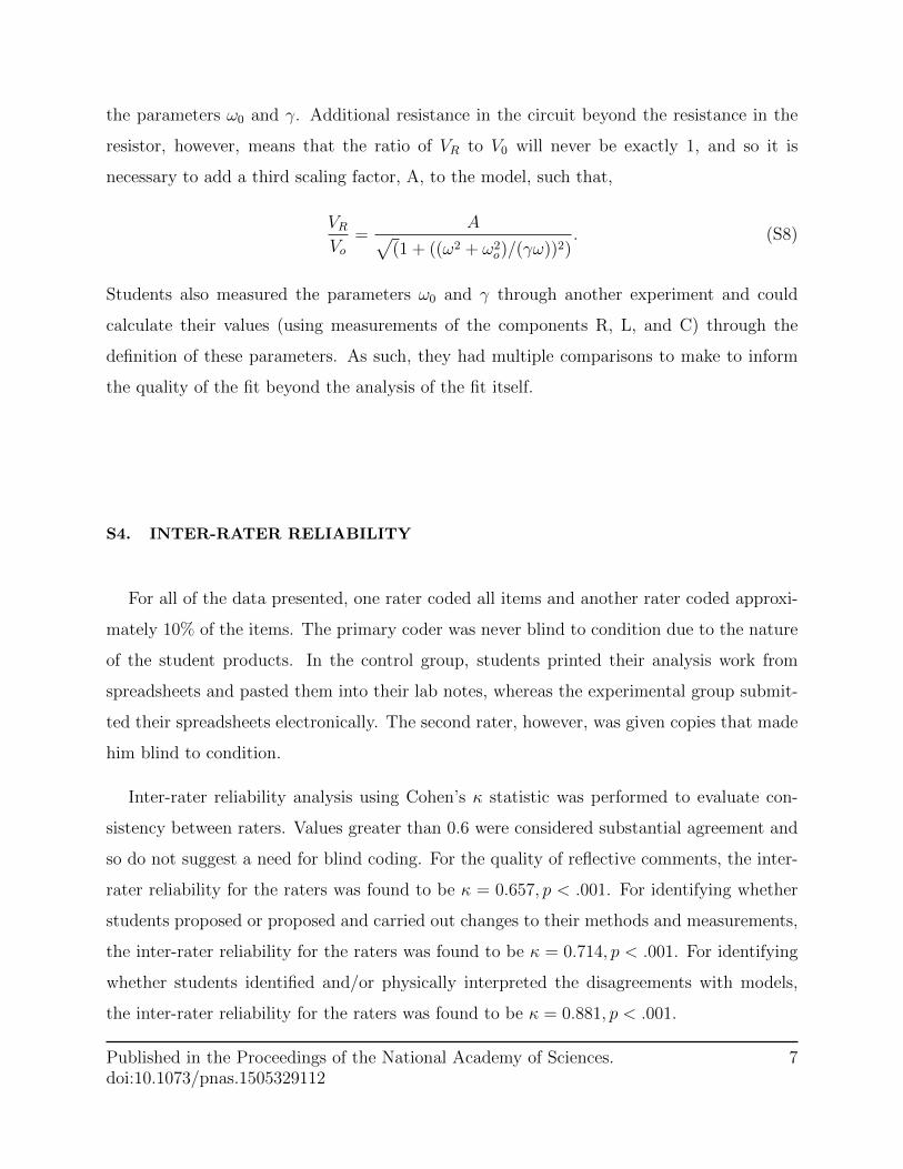
the parameters ω0 and γ. Additional resistance in the circuit beyond the resistance in the

resistor, however, means that the ratio of VR to V0 will never be exactly 1, and so it is

necessary to add a third scaling factor, A, to the model, such that,

VRVo

=A√

(1 + ((ω2 + ω2o)/(γω))2)

. (S8)

Students also measured the parameters ω0 and γ through another experiment and could

calculate their values (using measurements of the components R, L, and C) through the

definition of these parameters. As such, they had multiple comparisons to make to inform

the quality of the fit beyond the analysis of the fit itself.

S4. INTER-RATER RELIABILITY

For all of the data presented, one rater coded all items and another rater coded approxi-

mately 10% of the items. The primary coder was never blind to condition due to the nature

of the student products. In the control group, students printed their analysis work from

spreadsheets and pasted them into their lab notes, whereas the experimental group submit-

ted their spreadsheets electronically. The second rater, however, was given copies that made

him blind to condition.

Inter-rater reliability analysis using Cohen’s κ statistic was performed to evaluate con-

sistency between raters. Values greater than 0.6 were considered substantial agreement and

so do not suggest a need for blind coding. For the quality of reflective comments, the inter-

rater reliability for the raters was found to be κ = 0.657, p < .001. For identifying whether

students proposed or proposed and carried out changes to their methods and measurements,

the inter-rater reliability for the raters was found to be κ = 0.714, p < .001. For identifying

whether students identified and/or physically interpreted the disagreements with models,

the inter-rater reliability for the raters was found to be κ = 0.881, p < .001.


7

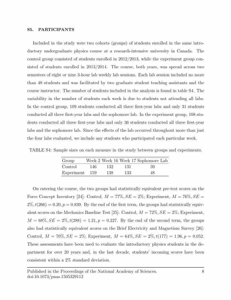
S5. PARTICIPANTS

Included in the study were two cohorts (groups) of students enrolled in the same intro-

ductory undergraduate physics course at a research-intensive university in Canada. The

control group consisted of students enrolled in 2012/2013, while the experiment group con-

sisted of students enrolled in 2013/2014. The course, both years, was spread across two

semesters of eight or nine 3-hour lab weekly lab sessions. Each lab session included no more

than 48 students and was facilitated by two graduate student teaching assistants and the

course instructor. The number of students included in the analysis is found in table S4. The

variability in the number of students each week is due to students not attending all labs.

In the control group, 109 students conducted all three first-year labs and only 31 students

conducted all three first-year labs and the sophomore lab. In the experiment group, 108 stu-

dents conducted all three first-year labs and only 36 students conducted all three first-year

labs and the sophomore lab. Since the effects of the lab occurred throughout more than just

the four labs evaluated, we include any students who participated each particular week.

TABLE S4: Sample sizes on each measure in the study between groups and experiments.

Group Week 2 Week 16 Week 17 Sophomore Lab

Control 146 132 131 39

Experiment 159 138 133 48

On entering the course, the two groups had statistically equivalent pre-test scores on the

Force Concept Inventory [24]: Control, M = 77%, SE = 2%; Experiment, M = 76%, SE =

2%, t(266) = 0.20, p = 0.839. By the end of the first term, the groups had statistically equiv-

alent scores on the Mechanics Baseline Test [25]: Control, M = 72%, SE = 2%; Experiment,

M = 68%, SE = 2%, t(288) = 1.21, p = 0.227. By the end of the second term, the groups

also had statistically equivalent scores on the Brief Electricity and Magnetism Survey [26]:

Control, M = 70%, SE = 2%; Experiment, M = 64%, SE = 2%, t(177) = 1.96, p = 0.052.

These assessments have been used to evaluate the introductory physics students in the de-

partment for over 20 years and, in the last decade, students’ incoming scores have been

consistent within a 2% standard deviation.


8

The critical thinking behaviours assessed in this study relate primarily to evaluating

data and physical measurement systems. The questions on the MBT and BEMA evaluate

students’ ability to apply specific physics concepts in idealized situations. There is very little

overlap between the knowledge and reasoning required to answer those questions, and the

real-world, data-driven critical thinking about data and measurement systems learned in

the lab course. We also would expect that the lecture and other components of the courses

would dominant over a possible effect related to the lab. Therefore, it is not surprising that

the scores are not correlated.

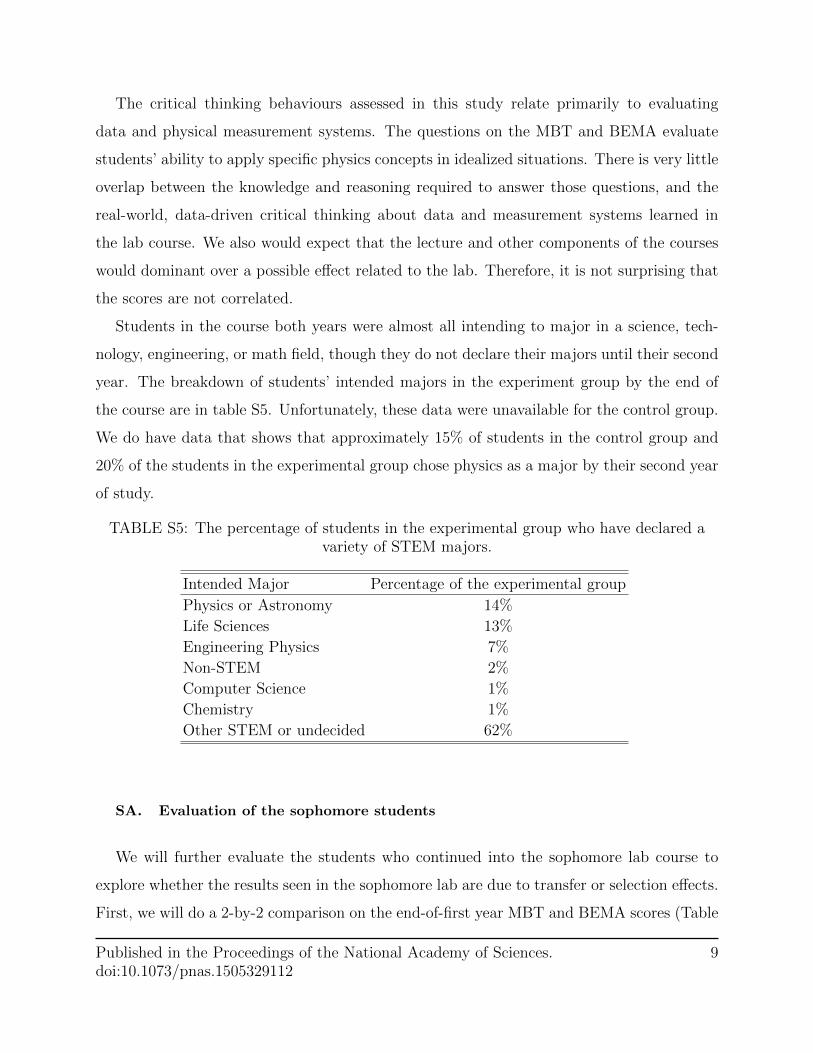
Students in the course both years were almost all intending to major in a science, tech-

nology, engineering, or math field, though they do not declare their majors until their second

year. The breakdown of students’ intended majors in the experiment group by the end of

the course are in table S5. Unfortunately, these data were unavailable for the control group.

We do have data that shows that approximately 15% of students in the control group and

20% of the students in the experimental group chose physics as a major by their second year

of study.

TABLE S5: The percentage of students in the experimental group who have declared avariety of STEM majors.

Intended Major Percentage of the experimental group

Physics or Astronomy 14%

Life Sciences 13%

Engineering Physics 7%

Non-STEM 2%

Computer Science 1%

Chemistry 1%

Other STEM or undecided 62%

SA. Evaluation of the sophomore students

We will further evaluate the students who continued into the sophomore lab course to

explore whether the results seen in the sophomore lab are due to transfer or selection effects.

First, we will do a 2-by-2 comparison on the end-of-first year MBT and BEMA scores (Table


9

S6), comparing between students who did and did not take the sophomore lab course and

between the experiment and control groups in the first-year course.

Overall, the students who went on to take the sophomore physics lab course outperformed

the students who did not take the sophomore lab, as measured on both the MBT and the

BEMA (note that, of the students in the control group, there was no difference between

students who did and did not take the sophomore lab course on the BEMA). This tells us

that the students in the sophomore physics labs generally had a stronger conceptual physics

background than the students who did not continue in an upper-year physics lab course.

This is consistent with the expected selection bias of students who choose to pursue more

physics courses. Of the students who took the sophomore physics lab, however, there is a

non-significant difference between the experimental and control groups on both the MBT and

BEMA. This is consistent with the overall lack of differences on these measures between the

full experiment and control conditions in the first-year lab course discussed in the previous

section.

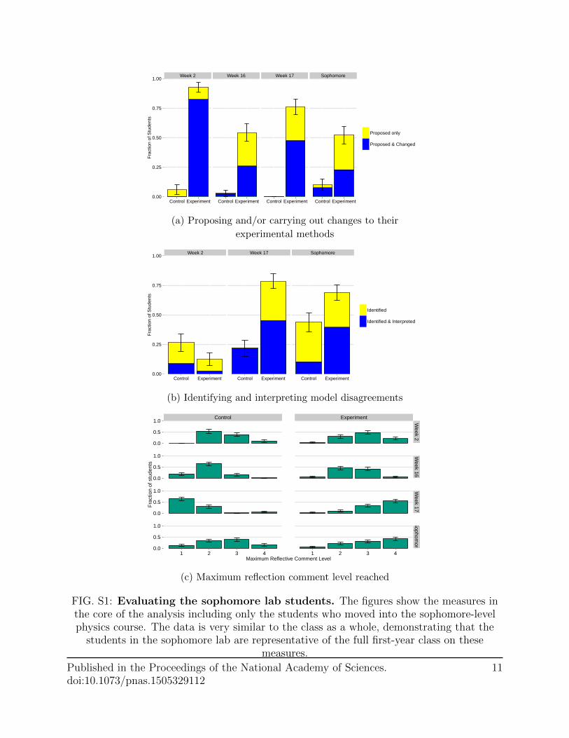
Next, we compare these two subgroups on their evaluation, iteration, and reflection be-

haviours throughout the first year labs. The trends in the figures S1b, S1a, and S1c showing

only the sophomore students are very similar to those for the whole course (figures 1, 2, and

3). This suggests that the students who continued into the the sophomore course were not

exceptional in their behaviours in first-year. This further suggests that the effect seen in the

Sophomore Lab experiment are not due to selection effects. It remains that the upwards

shift in the control group’s reflective comments and evaluation of the model are due to some-

thing inherent in the sophomore lab course. Most likely these shifts can be attributed to

the prompt in the instructions to explain why there may be extra parameters in the model.

This instruction would explain a shift in the model evaluation and reflective comments, but

not in iteration, as seen in the data.

S6. REFLECTION ANALYSIS

To analyze students’ reflection in the lab, we evaluated students’ reflective comments

associated with their statistical data analysis and conclusions. The reflective comments were


10

Week 2 Week 16 Week 17 Sophomore

0.00

0.25

0.50

0.75

1.00

Control Experiment Control Experiment Control Experiment Control Experiment

Fra

ctio

n of

Stu

dent

s

Proposed only

Proposed & Changed

(a) Proposing and/or carrying out changes to their

experimental methods

Week 2 Week 17 Sophomore

0.00

0.25

0.50

0.75

1.00

Control Experiment Control Experiment Control Experiment

Fra

ctio

n of

Stu

dent

s

Identified

Identified & Interpreted

(b) Identifying and interpreting model disagreements

Control Experiment

0.0

0.5

1.0

0.0

0.5

1.0

0.0

0.5

1.0

0.0

0.5

1.0

Week 2

Week 16

Week 17

Sophom

ore

1 2 3 4 1 2 3 4Maximum Reflective Comment Level

Fra

ctio

n of

stu

dent

s

(c) Maximum reflection comment level reached

FIG. S1: Evaluating the sophomore lab students. The figures show the measures inthe core of the analysis including only the students who moved into the sophomore-levelphysics course. The data is very similar to the class as a whole, demonstrating that the

students in the sophomore lab are representative of the full first-year class on thesemeasures.


11

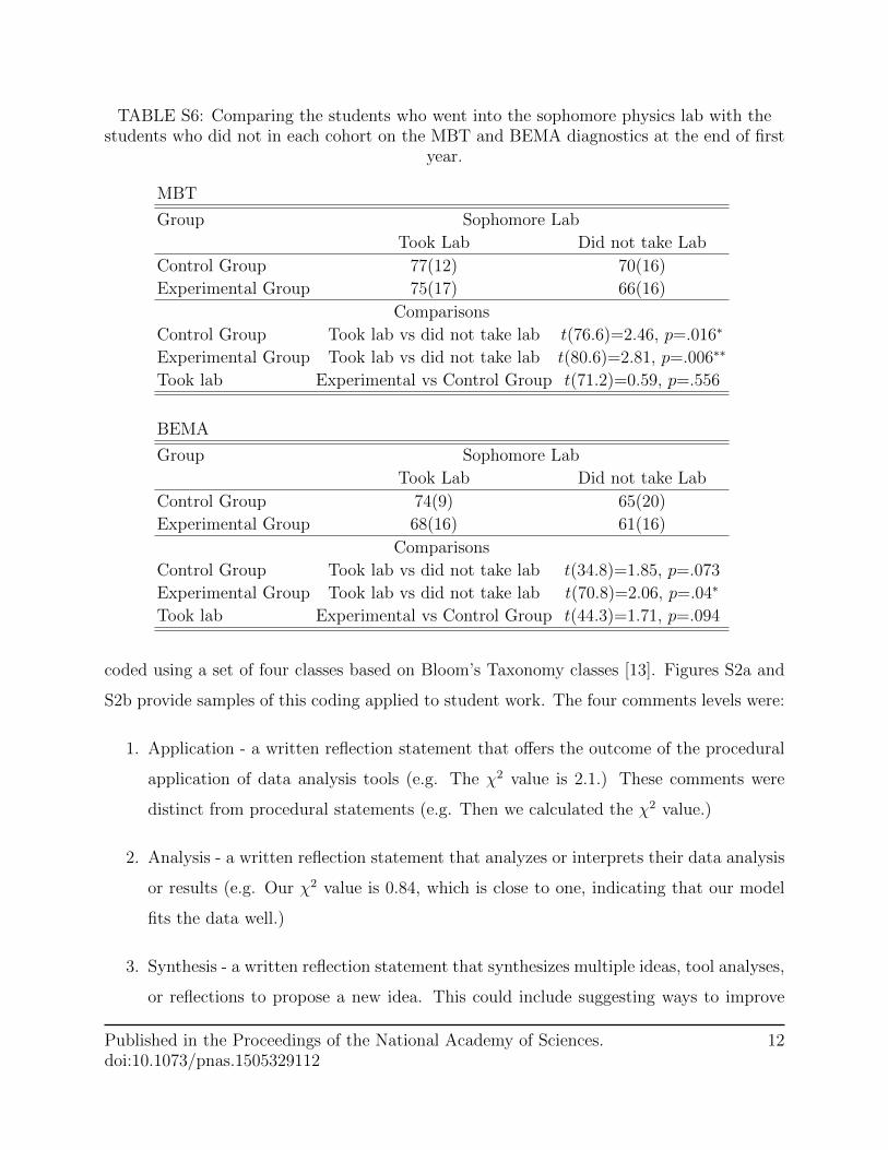
TABLE S6: Comparing the students who went into the sophomore physics lab with thestudents who did not in each cohort on the MBT and BEMA diagnostics at the end of first

year.

MBT

Group Sophomore Lab

Took Lab Did not take Lab

Control Group 77(12) 70(16)

Experimental Group 75(17) 66(16)

Comparisons

Control Group Took lab vs did not take lab t(76.6)=2.46, p=.016∗

Experimental Group Took lab vs did not take lab t(80.6)=2.81, p=.006∗∗

Took lab Experimental vs Control Group t(71.2)=0.59, p=.556

BEMA

Group Sophomore Lab

Took Lab Did not take Lab

Control Group 74(9) 65(20)

Experimental Group 68(16) 61(16)

Comparisons

Control Group Took lab vs did not take lab t(34.8)=1.85, p=.073

Experimental Group Took lab vs did not take lab t(70.8)=2.06, p=.04∗

Took lab Experimental vs Control Group t(44.3)=1.71, p=.094

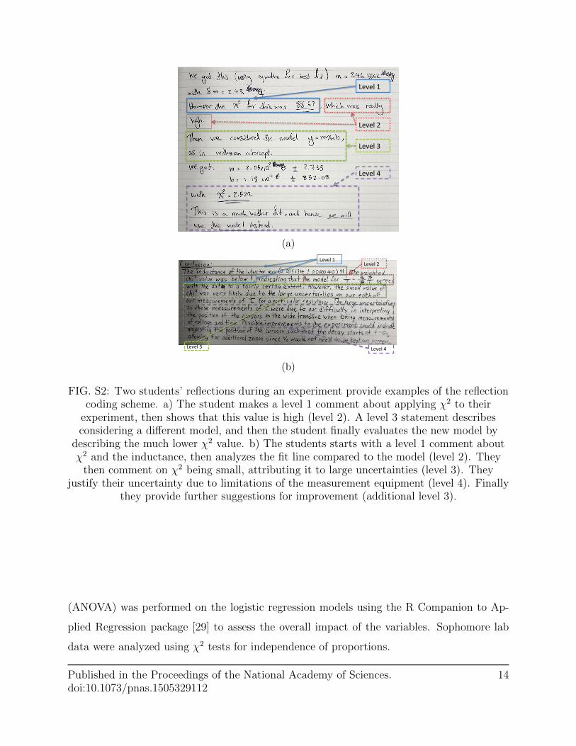
coded using a set of four classes based on Bloom’s Taxonomy classes [13]. Figures S2a and

S2b provide samples of this coding applied to student work. The four comments levels were:

1. Application - a written reflection statement that offers the outcome of the procedural

application of data analysis tools (e.g. The χ2 value is 2.1.) These comments were

distinct from procedural statements (e.g. Then we calculated the χ2 value.)

2. Analysis - a written reflection statement that analyzes or interprets their data analysis

or results (e.g. Our χ2 value is 0.84, which is close to one, indicating that our model

fits the data well.)

3. Synthesis - a written reflection statement that synthesizes multiple ideas, tool analyses,

or reflections to propose a new idea. This could include suggesting ways to improve


12

measurements (e.g. we will take more data in this range, since the data is sparse) or

models (e.g. our data has an intercept so the model should have an intercept), as well

as making comparisons (e.g. The χ2 value for the y = mx fit was 43.8, but for the

y = mx+ b fit χ2 was 4.17, which is much smaller.)

4. Evaluation - a written reflection statement that evaluates, criticizes, or judges the

previous ideas presented. Evaluation can look similar to analysis, but the distinction

is that evaluation must follow a synthesis comment. For example, after a synthesis that

compared two different models and demonstrated that adding an intercept lowered the

χ2 value, an evaluation could follow as, “...the intercept was necessary due, most likely,

to the inherent resistance within the circuit (such as in the wires).”

Figures S2a and S2b demonstrate how the coding scheme is applied to three excerpts

from students’ books in the LR experiment (week 17). Each of the levels build on each

other, so a student making a level 4 evaluation statement would also have made lower level

statements, though level 1 comments (application) need not be present. While it is important

that students reflect on various parts of the data analysis, the results presented in the main

text examine the maximum reflection level a student reached. It should be noted that the

comments were not evaluated on correctness.

S7. ANALYSIS

For the first-year experiments, generalized linear mixed-effects models were performed us-

ing R [27] and and the Linear Mixed-Effects Models using ‘Eigen’ and S4 package [28] to ana-

lyze all three outcome measures (proposing and/or carrying out measurement changes, iden-

tifying and/or interpreting disagreements with models, and levels of reflection/comments).

For measurement changes and evaluating models, logistic regression analysis was performed

due to the dichotomous nature of the outcome variables. For the reflection data, Poisson

regression was used due to account for the bounded nature of the outcome variables. All

three analyses used condition, lab week, and the interaction between condition and lab week

as fixed effects and Subject ID as a random effects intercept. Type 3 analysis of variance


13

Level%1%

Level%2%

Level%3%

Level%4%

(a)

Level%1%Level%2%

Level%3% Level%4%

(b)

FIG. S2: Two students’ reflections during an experiment provide examples of the reflectioncoding scheme. a) The student makes a level 1 comment about applying χ2 to their

experiment, then shows that this value is high (level 2). A level 3 statement describesconsidering a different model, and then the student finally evaluates the new model by

describing the much lower χ2 value. b) The students starts with a level 1 comment aboutχ2 and the inductance, then analyzes the fit line compared to the model (level 2). They

then comment on χ2 being small, attributing it to large uncertainties (level 3). Theyjustify their uncertainty due to limitations of the measurement equipment (level 4). Finally

they provide further suggestions for improvement (additional level 3).

(ANOVA) was performed on the logistic regression models using the R Companion to Ap-

plied Regression package [29] to assess the overall impact of the variables. Sophomore lab

data were analyzed using χ2 tests for independence of proportions.


14

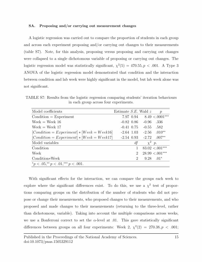
SA. Proposing and/or carrying out measurement changes

A logistic regression was carried out to compare the proportion of students in each group

and across each experiment proposing and/or carrying out changes to their measurements

(table S7). Note, for this analysis, proposing versus proposing and carrying out changes

were collapsed to a single dichotomous variable of proposing or carrying out changes. The

logistic regression model was statistically significant, χ2(5) = 470.55, p < .001. A Type 3

ANOVA of the logistic regression model demonstrated that condition and the interaction

between condition and lab week were highly significant in the model, but lab week alone was

not significant.

TABLE S7: Results from the logistic regression comparing students’ iteration behavioursin each group across four experiments.

Model coefficients Estimate S.E. Wald z p

Condition = Experiment 7.97 0.94 8.49 <.0001∗∗∗

Week = Week 16 -0.82 0.86 -0.96 .336

Week = Week 17 -0.41 0.75 -0.55 .582

[Condition = Experiment] ∗ [Week = Week16] -2.64 1.03 -2.56 .010∗∗

[Condition = Experiment] ∗ [Week = Week17] -2.54 0.93 -2.72 .007∗∗

Model variables df χ2 p.

Condition 1 83.02 <.001∗∗∗

Week 2 28.99 <.001∗∗∗

Condition∗Week 2 9.28 .01∗

∗p < .05,∗∗ p < .01,∗∗∗ p < .001.

With significant effects for the interaction, we can compare the groups each week to

explore where the significant differences exist. To do this, we use a χ2 test of propor-

tions comparing groups on the distribution of the number of students who did not pro-

pose or change their measurements, who proposed changes to their measurements, and who

proposed and made changes to their measurements (returning to the three-level, rather

than dichotomous, variable). Taking into account the multiple comparisons across weeks,

we use a Bonferroni correct to set the α-level at .01. This gave statistically significant

differences between groups on all four experiments: Week 2, χ2(2) = 270.38, p < .001;


15

Week 16, χ2(2) = 107.51, p < .001; Week 17, χ2(2) = 128.39, p < .001; Sophomore Lab,

χ2(2) = 17.58, p < .001. This demonstrates that the experiment group outperformed the

control group on this measure on all experiments.

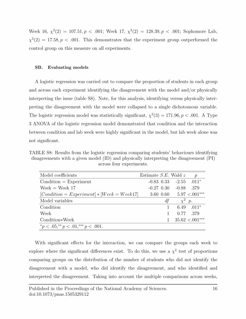
SB. Evaluating models

A logistic regression was carried out to compare the proportion of students in each group

and across each experiment identifying the disagreement with the model and/or physically

interpreting the issue (table S8). Note, for this analysis, identifying versus physically inter-

preting the disagreement with the model were collapsed to a single dichotomous variable.

The logistic regression model was statistically significant, χ2(3) = 171.96, p < .001. A Type

3 ANOVA of the logistic regression model demonstrated that condition and the interaction

between condition and lab week were highly significant in the model, but lab week alone was

not significant.

TABLE S8: Results from the logistic regression comparing students’ behaviours identifyingdisagreements with a given model (ID) and physically interpreting the disagreement (PI)

across four experiments.


Condition = Experiment -0.83 0.33 -2.55 .011∗

Week = Week 17 -0.27 0.30 -0.88 .379

[Condition = Experiment] ∗ [Week = Week17] 3.60 0.60 5.97 <.001∗∗∗


Condition 1 6.49 .011∗

Week 1 0.77 .379

Condition∗Week 1 35.62 <.001∗∗∗

∗p < .05,∗∗ p < .01,∗∗∗ p < .001.

With significant effects for the interaction, we can compare the groups each week to

explore where the significant differences exist. To do this, we use a χ2 test of proportions

comparing groups on the distribution of the number of students who did not identify the

disagreement with a model, who did identify the disagreement, and who identified and

interpreted the disagreement. Taking into account the multiple comparisons across weeks,


16

we use a Bonferroni correct to set the α-level at .02. This gave significant differences between

groups on all three experiments: Week 2, χ2(2) = 8.60, p = .014; Week 17, χ2(2) = 99.04, p <

.001; Sophomore Lab, χ2(2) = 10.32, p = .006.

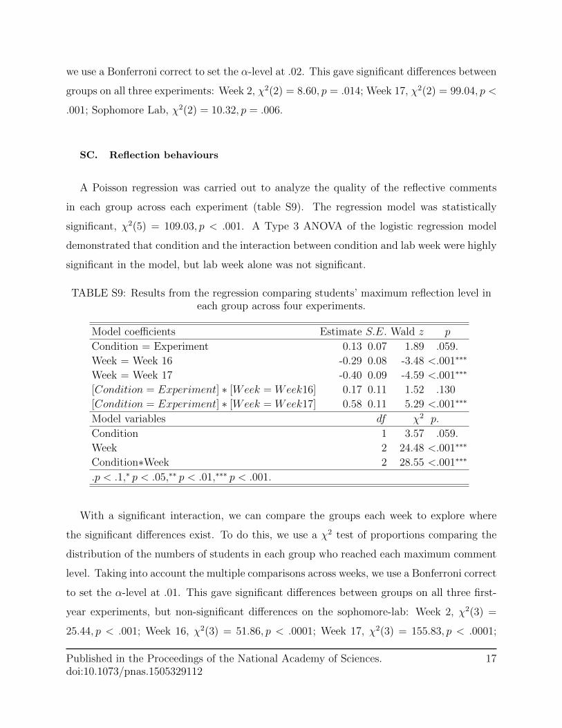
SC. Reflection behaviours

A Poisson regression was carried out to analyze the quality of the reflective comments

in each group across each experiment (table S9). The regression model was statistically

significant, χ2(5) = 109.03, p < .001. A Type 3 ANOVA of the logistic regression model

demonstrated that condition and the interaction between condition and lab week were highly

significant in the model, but lab week alone was not significant.

TABLE S9: Results from the regression comparing students’ maximum reflection level ineach group across four experiments.


Condition = Experiment 0.13 0.07 1.89 .059.

Week = Week 16 -0.29 0.08 -3.48 <.001∗∗∗

Week = Week 17 -0.40 0.09 -4.59 <.001∗∗∗

[Condition = Experiment] ∗ [Week = Week16] 0.17 0.11 1.52 .130

[Condition = Experiment] ∗ [Week = Week17] 0.58 0.11 5.29 <.001∗∗∗


Condition 1 3.57 .059.

Week 2 24.48 <.001∗∗∗

Condition∗Week 2 28.55 <.001∗∗∗

.p < .1,∗ p < .05,∗∗ p < .01,∗∗∗ p < .001.

With a significant interaction, we can compare the groups each week to explore where

the significant differences exist. To do this, we use a χ2 test of proportions comparing the

distribution of the numbers of students in each group who reached each maximum comment

level. Taking into account the multiple comparisons across weeks, we use a Bonferroni correct

to set the α-level at .01. This gave significant differences between groups on all three first-

year experiments, but non-significant differences on the sophomore-lab: Week 2, χ2(3) =

25.44, p < .001; Week 16, χ2(3) = 51.86, p < .0001; Week 17, χ2(3) = 155.83, p < .0001;


17

Sophomore Lab, χ2(3) = 7.58, p = .056.

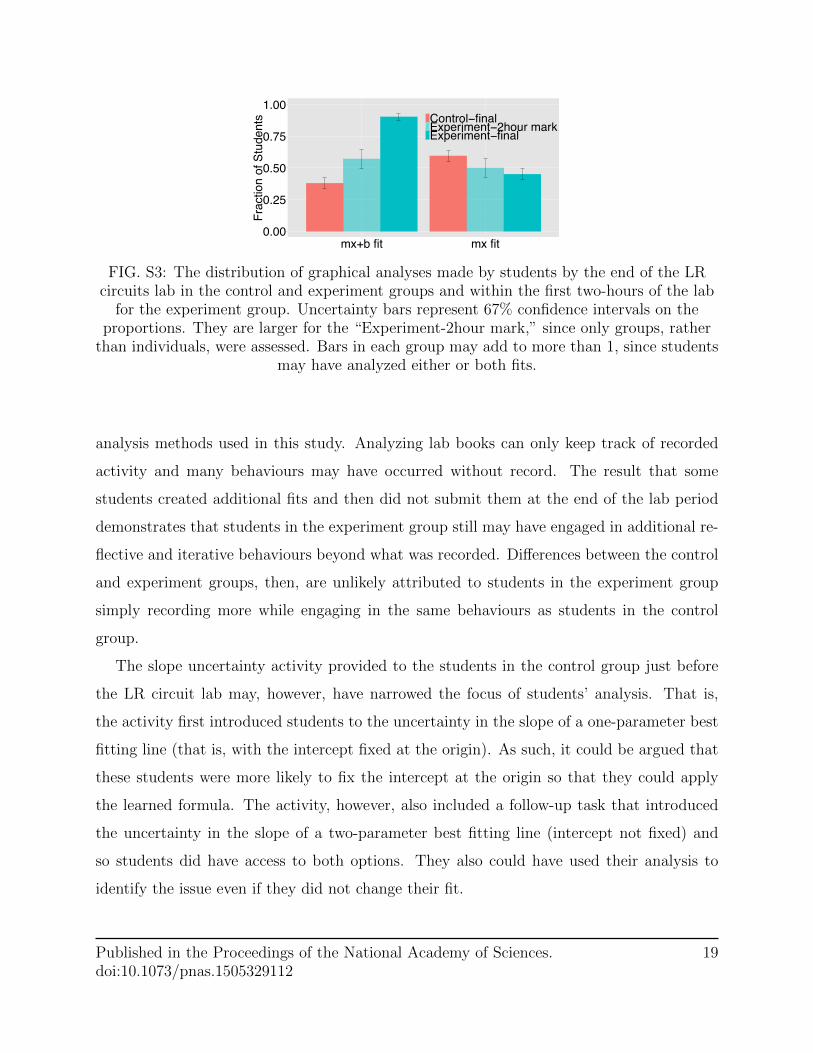
S8. TIME ON TASK IN THE LR EXPERIMENT

One confounding issue to the week 17 LR circuit experiment was that students in the

control group worked through a computer-based inquiry activity at the beginning of the

experiment session. The activity taught students how to calculate the uncertainty in the

slope of a best-fitting line, which they also used to reanalyze the previous week’s data.

As such, the control group spent approximately two hours on the LR circuit lab, whereas

the experiment group spent three hours. Not having enough time to reflect on data and

act on that reflection may explain the different outcomes observed in the main text. As a

precautionary measure, we observed students in the experiment group two-hours into the lab

session to evaluate what analysis they had performed by that time. The observer recorded

whether the group had by that time produced a one-parameter mx fit or a two-parameter

mx+ b fit.

The results, shown in figure S3, demonstrate that if the students in the experiment group

had been given the same amount of time on task as students in the control group, more of

them still would have made the modification to the model and included an intercept in their

fit. Given additional time, however, even more students were able to think critically about

the task and make better sense of their data. From this result, we conclude that the effects

seen in this experiment are still primarily due to students’ overall improved behaviours.

Indeed, the effect is much larger due to the additional time, which is an important feature of

the intervention itself. It takes time for students to engage deeply in a task, think critically,

and solve any problems that arise [30]. Comparing between students in the experiment group

at the 2-hour mark and the final 3-hour mark demonstrates the striking effect that an extra

hour can make to students’ productivity.

The number of single-parameter mx fits decreased slightly from the 2-hour observations

and the final submitted materials for the experiment group. This could have occurred if

students recognized that the mx fit was not helpful in understanding their data, due to the

additional intercept required. This is interesting to note in light of the limitations of the


18

0.00

0.25

0.50

0.75

1.00

mx+b fit mx fitFr

actio

n of

Stu

dent

s Control−finalExperiment−2hour markExperiment−final

FIG. S3: The distribution of graphical analyses made by students by the end of the LRcircuits lab in the control and experiment groups and within the first two-hours of the lab

for the experiment group. Uncertainty bars represent 67% confidence intervals on theproportions. They are larger for the “Experiment-2hour mark,” since only groups, rather

than individuals, were assessed. Bars in each group may add to more than 1, since studentsmay have analyzed either or both fits.

analysis methods used in this study. Analyzing lab books can only keep track of recorded

activity and many behaviours may have occurred without record. The result that some

students created additional fits and then did not submit them at the end of the lab period

demonstrates that students in the experiment group still may have engaged in additional re-

flective and iterative behaviours beyond what was recorded. Differences between the control

and experiment groups, then, are unlikely attributed to students in the experiment group

simply recording more while engaging in the same behaviours as students in the control

group.

The slope uncertainty activity provided to the students in the control group just before

the LR circuit lab may, however, have narrowed the focus of students’ analysis. That is,

the activity first introduced students to the uncertainty in the slope of a one-parameter best

fitting line (that is, with the intercept fixed at the origin). As such, it could be argued that

these students were more likely to fix the intercept at the origin so that they could apply

the learned formula. The activity, however, also included a follow-up task that introduced

the uncertainty in the slope of a two-parameter best fitting line (intercept not fixed) and

so students did have access to both options. They also could have used their analysis to

identify the issue even if they did not change their fit.


19

Documents

Enseñar Pensamiento Critico Ingles 1508.04870v1