Efficient Long-term Mapping in Dynamic Environments

Marıa T. Lazaro, Roberto Capobianco and Giorgio Grisetti

Abstract— As autonomous robots are increasingly being in-troduced in real-world environments operating for long periodsof time, the difficulties of long-term mapping are attractingthe attention of the robotics research community. This paperproposes a full SLAM system capable of handling the dynamicsof the environment across a single or multiple mapping sessions.

Using the pose graph SLAM paradigm, the system works onlocal maps in the form of 2D point cloud data which are updatedover time to store the most up-to-date state of the environment.The core of our system is an efficient ICP-based alignmentand merging procedure working on the clouds that copes withnon-static entities of the environment. Furthermore, the systemretains the graph complexity by removing out-dated nodesupon robust inter- and intra-session loop closure detectionswhile graph coherency is preserved by using condensed mea-surements. Experiments conducted with real data from long-term SLAM datasets demonstrate the efficiency, accuracy andeffectiveness of our system in the management of the mappingproblem during long-term robot operation.

I. INTRODUCTION

In the last years, robots have been progressively intro-duced in public environments where space is shared withhumans, such as shopping centers [1], airports [2], eldercare homes [3], hospitals or museums. In order to navigateautonomously these environments, robots require a mapof the building in which they have to operate. This mapis usually obtained before the deployment of the robotsby using Simultaneous Localization and Mapping (SLAM)techniques, for which reliable implementations are publiclyavailable [4], [5], [6].

Typically, mapping public environments presents severalchallenges. First, despite the risk of introducing artifacts inthe final map, data acquisition can rarely be executed inthe absence of people. This constitutes a highly dynamicsituation that makes the environment non-stationary, andmust be handled by the SLAM system within the activemapping session. Second, even when a proper data ac-quisition is realized (e.g., with the building closed to thepublic), the obtained map might not be usable after few days,due to substantial changes in the environment (e.g., movedstands, new decorations for special events, etc). Nevertheless,after a reconfiguration, the map might be still valid forsome time. Hence, we refer to this sort of environments –affected by low dynamics – as semi-static. The changes insemi-static environments might affect the topology of theenvironment and substantially influence its local appearance,

Marıa T. Lazaro, Roberto Capobianco and Giorgio Grisetti are withDipartimento di Ingegneria Informatica Automatica e Gestionale ”An-tonio Ruberti”, Sapienza University of Rome, Italy. mtlazaro,capobianco, grisetti@diag.uniroma1.it

thus invalidating portions of the previously acquired map thathave to be estimated from scratch.

Although dealing with dynamic and semi-static environ-ments in a life-long mapping process is one of the goals ofmobile robotics, typical solutions are impractical since theyrequire to acquire a completely new map of the whole envi-ronment whenever a semi-static change occurs. Conversely,it would be sufficient to update only the portion of the mapthat changed.

Most of the latest successful solutions to the SLAMproblem are based on a pose graph representation whosenodes store discretized positions along the robot trajectoryand edges encode relations between nodes. Using this repre-sentation, the SLAM problem simplifies to the resolution ofan optimization problem whose complexity depends directlyon the number of nodes present in the graph.

When considering this problem from a life-long perspec-tive, a robot navigating continuously the environment willproduce a limitless addition of nodes, making the optimiza-tion problem intractable. Directly related with the numberof nodes is also the problem of loop closure detection. Theunbounded addition of nodes will increase the dimension ofthe search for possible candidates and, with it, the possibleinclusion of false positives. Furthermore, inconsistenciesbetween the current state of the environment and what ispresent in the map due to the changing environment canlead to mislocalization or navigation errors.

Therefore, there are two main aspects to be considered inorder to ensure the correct operation of a SLAM system in along-term horizon: the maintenance of a constrained dimen-sion of its inherent optimization problem and an efficientmanagement of the changes that happen over time.

This paper presents a full SLAM system focused on themanagement of long-term situations capable of handling bothhighly dynamic situations within a mapping session and mapupdates within multiple sessions to cope with low dynamics.Our system estimates a map as a pose graph whose nodescontain local maps which allows to maintain a sparser graphrepresentation. Local maps store the appearance informationin the form of 2D point clouds while spatial relationsbetween adjacent local maps are encoded as a graph edges.The use of point clouds offers higher definition and are lessmemory demanding than other data structures such as gridswhich can only represent the environment up to a certainresolution to maintain performance constraints. The coreof our system is the use of an effective ICP-based pointcloud alignment and merging procedure that allows to updatethe content of the local maps to preserve the most up-to-date information about the environment. Graph complexity

is retained bounded by removing nodes containing out-datedinformation, while the graph coherency is preserved bycompressing prior knowledge through condensed measure-ments [7]. Map information obtained over different sessionsis managed by the same graph structure obtaining a balancebetween simplicity and effectiveness in determining bothintra- and inter-session loop closures.

We release our system as open source1 which providesROS compatibility and visualization tools.

II. RELATED WORK

The problem of the dimensionality in SLAM is wellknown and a variety of techniques have been proposed overthe years to overcome such issue. Solutions range from thosestudying the structure of the optimization problem [8], [9]to those based on graph reduction methods [10], [11].

In [12], a framework for multi-session map optimiza-tion is proposed, where several independently optimizedpose-graphs acquired at different sessions are combined byusing anchor nodes. While graph reduction methods arenormally batch algorithms executed off-line (i.e., using asinput an already constructed graph), their on-line applicationis not straightforward. The SLAM system proposed in [13]achieves long-term operation by using a reduced graph whichretains bounded complexity over time proportional to the ex-plored environment and not the total distance traveled. Newnodes are added only if there are not previous nodes nearby,while new information from loop closures is incorporatedas new edges between existing poses. However, the systemdoes not update the sensor data contained in the nodes toconsider the dynamic changes of the environment.

Regarding the works considering the non-static natureof the environment, the tendency is to maintain parallelmaps, one for short-term periods characterized by highdynamics and another one for long-term periods capturingmore stationary structures. Early works [14], [15] used agrid-based map representation to that end while Biber andDuckett [16] extended this perspective by maintaining notjust two short- and long-term maps but by tracking andupdating the state of the environment at multiple timescales.Also based on grid-based mapping [4], is the recent work byKrajnik et al. [17]. Their system builds a new map for eachrun, while consistency between sessions is achieved by usinglocalization with respect the previous model as odometrymeasurements for the current session. Maps are integratedinto a spatio-temporal model capturing the persistency andperiodicity of the environment that allows to predict thefuture state of the environment with proven usefulness fornavigation and path planning purposes.

In a more recent graph-based approach [18], Labbe andMichaud organize graph nodes in Short-term, Long-term andWorking memories. Nodes are moved from one type of mem-ory to another as they are required as in a cache mechanism.Also based on graph-based representation, Walcott-Bryant etal. [19] proposed a ”Dynamic Pose Graph (DPG)” focused

1https://gitlab.com/srrg-software/srrg mapper2d

2D Cloud

Merging

Vertex

Merging

Long-term Map Maintenance

Odometry

Local Map

MaintenanceICP

Normals

extraction

Local Mapper

Laser scans(2D point cloud)

Robust

Loop Closure

Front-end

Graph SLAM

g2o

Back-end

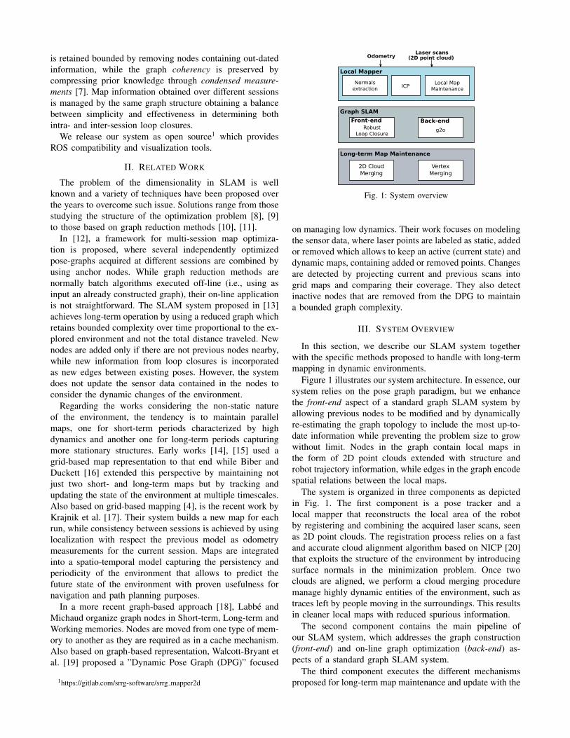
Fig. 1: System overview

on managing low dynamics. Their work focuses on modelingthe sensor data, where laser points are labeled as static, addedor removed which allows to keep an active (current state) anddynamic maps, containing added or removed points. Changesare detected by projecting current and previous scans intogrid maps and comparing their coverage. They also detectinactive nodes that are removed from the DPG to maintaina bounded graph complexity.

III. SYSTEM OVERVIEW

In this section, we describe our SLAM system togetherwith the specific methods proposed to handle with long-termmapping in dynamic environments.

Figure 1 illustrates our system architecture. In essence, oursystem relies on the pose graph paradigm, but we enhancethe front-end aspect of a standard graph SLAM system byallowing previous nodes to be modified and by dynamicallyre-estimating the graph topology to include the most up-to-date information while preventing the problem size to growwithout limit. Nodes in the graph contain local maps inthe form of 2D point clouds extended with structure androbot trajectory information, while edges in the graph encodespatial relations between the local maps.

The system is organized in three components as depictedin Fig. 1. The first component is a pose tracker and alocal mapper that reconstructs the local area of the robotby registering and combining the acquired laser scans, seenas 2D point clouds. The registration process relies on a fastand accurate cloud alignment algorithm based on NICP [20]that exploits the structure of the environment by introducingsurface normals in the minimization problem. Once twoclouds are aligned, we perform a cloud merging proceduremanage highly dynamic entities of the environment, such astraces left by people moving in the surroundings. This resultsin cleaner local maps with reduced spurious information.

The second component contains the main pipeline ofour SLAM system, which addresses the graph construction(front-end) and on-line graph optimization (back-end) as-pects of a standard graph SLAM system.

The third component executes the different mechanismsproposed for long-term map maintenance and update with the

most current information about the environment considering,therefore, dynamics between multiple mapping sessions.

A. Local Mapper

In this work, we use a variant of the NICP algorithmintroduced by Serafin et al. [20] to perform 2D point cloudregistration. To this end, we define a 2D point cloud P =p1:N as a set of extended points p composed of a pointp = (px py)T and its normal n = (nx ny)T . In computingsuch normal, we consider the neighborhood Di of eachpoint pi and compute the covariance matrix of the GaussiandistributionN (µi,Σi) of the points lying in Di, and set ni tobe the eigenvector corresponding to the smallest eigenvalueof the covariance matrix Σi.

Given an extended point p we can apply the compositionoperator ⊕ to transform the extended point by using atransformation matrix T composed of a rotation R and atranslation vector t as

p = (p,n)T T⊕ p = (Rp + t,Rn) (1)

Furthermore, we define a projection function s = π(p)that maps a Cartesian point p to range and bearing spaces = (r, α), i.e., the laser measurement space. Accordingly,we can define a back-projection function p = π−1(s) thatenables us to retrieve the two-dimensional Cartesian point pfrom s. By using this function, we can represent a laser scanas a cloud of extended points obtained by back-projectingthe set of measurements s1:N to a set of points p1:Nin the Cartesian space and by computing, for each pi, thecorresponding point normal ni.

1) Cloud registration: Given two extended point cloudsPr = pr

1:Nr and Pc = pc

1:Nc, we use a set C =

(i, j)1:M of correspondences between extended points pri

and pcj , to compute the transformation matrix T∗ that mini-

mizes the distance between corresponding points, expressedas the following least squares objective function:

T∗ = argminT

∑C

(T⊕ pci − pr

j)T Ωi,j(T⊕ pc

i − prj). (2)

where, Ωi,j = diag(Ωpi,j ,Ω

ni,j) is an information matrix that

takes into account the noise properties of the sensor andsummarizes the contributions of the information Ωp

i,j andΩn

i,j , respectively coming from the point and normal cor-respondences. Finally, in order to obtain the transformationT∗, we solve Eq. 2 iteratively by using a damped versionof the Gauss-Newton algorithm. During optimization we usethe robot odometry To both as initial guess and as prior. Inthis way we restrict the solution returned by the solver to liein the confidence ellipsoid of the odometry estimate.

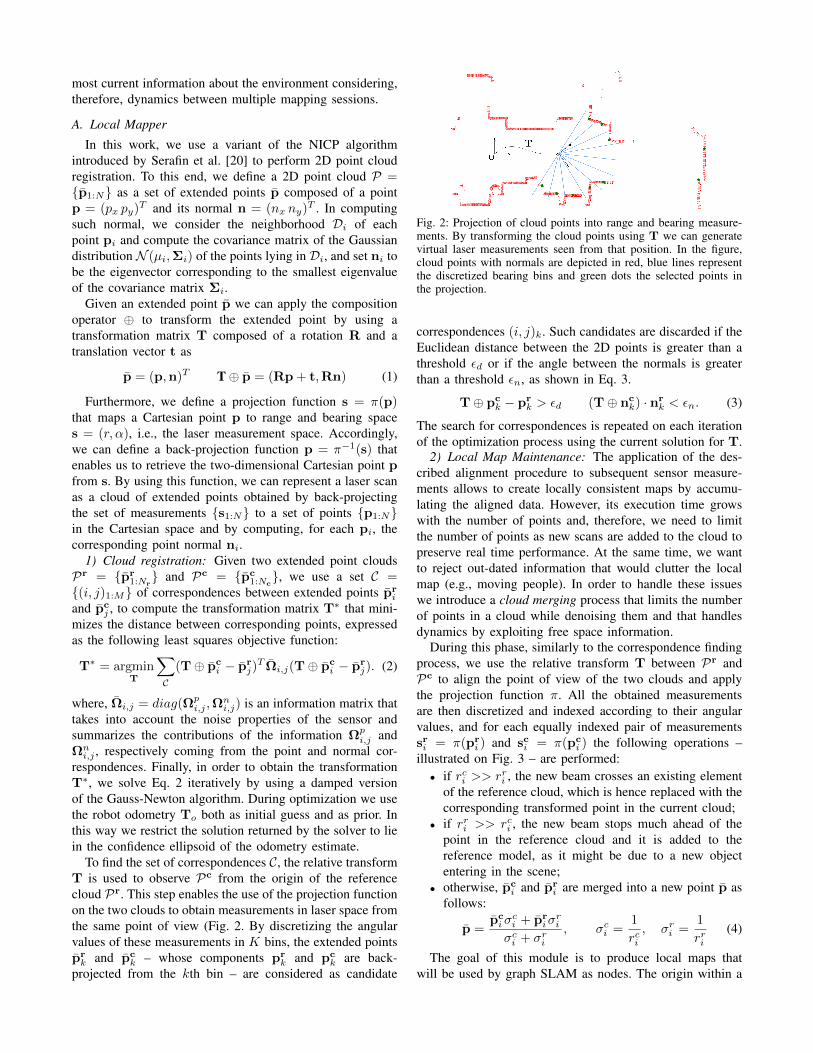
To find the set of correspondences C, the relative transformT is used to observe Pc from the origin of the referencecloud Pr. This step enables the use of the projection functionon the two clouds to obtain measurements in laser space fromthe same point of view (Fig. 2. By discretizing the angularvalues of these measurements in K bins, the extended pointsprk and pc

k – whose components prk and pc

k are back-projected from the kth bin – are considered as candidate

Fig. 2: Projection of cloud points into range and bearing measure-ments. By transforming the cloud points using T we can generatevirtual laser measurements seen from that position. In the figure,cloud points with normals are depicted in red, blue lines representthe discretized bearing bins and green dots the selected points inthe projection.

correspondences (i, j)k. Such candidates are discarded if theEuclidean distance between the 2D points is greater than athreshold εd or if the angle between the normals is greaterthan a threshold εn, as shown in Eq. 3.

T⊕ pck − pr

k > εd (T⊕ nck) · nr

k < εn. (3)

The search for correspondences is repeated on each iterationof the optimization process using the current solution for T.

2) Local Map Maintenance: The application of the des-cribed alignment procedure to subsequent sensor measure-ments allows to create locally consistent maps by accumu-lating the aligned data. However, its execution time growswith the number of points and, therefore, we need to limitthe number of points as new scans are added to the cloud topreserve real time performance. At the same time, we wantto reject out-dated information that would clutter the localmap (e.g., moving people). In order to handle these issueswe introduce a cloud merging process that limits the numberof points in a cloud while denoising them and that handlesdynamics by exploiting free space information.

During this phase, similarly to the correspondence findingprocess, we use the relative transform T between Pr andPc to align the point of view of the two clouds and applythe projection function π. All the obtained measurementsare then discretized and indexed according to their angularvalues, and for each equally indexed pair of measurementssri = π(pr

i ) and sci = π(pci ) the following operations –

illustrated on Fig. 3 – are performed:• if rci >> rri , the new beam crosses an existing element

of the reference cloud, which is hence replaced with thecorresponding transformed point in the current cloud;

• if rri >> rci , the new beam stops much ahead of thepoint in the reference cloud and it is added to thereference model, as it might be due to a new objectentering in the scene;

• otherwise, pci and pr

i are merged into a new point p asfollows:

p =pciσ

ci + pr

iσri

σci + σr

i

, σci =

1

rci, σr

i =1

rri(4)

The goal of this module is to produce local maps thatwill be used by graph SLAM as nodes. The origin within a

Fig. 3: Cloud points merging. Distances between points from thecurrent cloud (green) and the reference cloud (red) that have beenprojected into the same angular bin are analyzed. On the left beam,a new point falls in front the old one (rri >> rci ) and it is addedinto the cloud. On the right beam, a new point goes through theold one (rci >> rri ), thus the new point replaces the old one. Onthe middle, points are close each other, then they are merged intoone new point using Eq. 4.

Fig. 4: 2D cloud with trajectory. Current node xk and its associatedcloud are depicted in red while purple squares are the waypointsrepresenting the portion of the trajectory between nodes xk andxk−1. Relative transformations xk

i,k are stored in the cloud.

local map is selected to be the current pose of the robot in thetrajectory. Using local maps instead of raw scans to constructthe graph results in much smaller graphs, at the cost of losingvaluable information that is retained in the trajectory. Thismight ultimately lead to the inability to modify or ”deform”a local map. As a trade-off we still preserve the informationabout the robot trajectory within the local maps. To this end,we store in the local maps a discretized set of trajectory’swaypoints expressed with respect to the origin of the localmap. These waypoints represent vantage points from wherewe can render scans to produce other data like, for example,occupancy grid maps. More in detail, we store the relativetransformation xk

i,k with respect to the current node positionxk for each waypoint xi,k, i = 1, ...,m belonging to thediscretized portion of the trajectory between nodes xk andxk−1. This is illustrated on Fig. 4.

B. Graph SLAM

Our system uses as a basis a pose-graph for map repre-sentation. This graph is composed of nodes containing robotpositions and edges encoding spatial relations between thenodes. More formally, let us denote as x = (x1, ...,xn)T theset of nodes representing the robot trajectory and zij as themeasurement encoded in an edge connecting two nodes xi

and xj , affected by Gaussian noise with information matrix

Ωij . Let also be h(xi,xj) the function that computes therelative relation between the nodes xi and xj given theircurrent state. The estimation error eij given the measurementzij can be calculated as:

eij = zij − h(xi,xj) (5)

The solution of a graph-based SLAM approach minimizesthe overall error to obtain a configuration of the nodes x∗

that better explain the set of measurements:

x∗ = argminx

∑i,j

eTijΩijeij (6)

The above Eq. 6 represents the SLAM problem as a Least-Squares optimization problem that can be solved using iter-ative methods like Gauss-Newton or Levenberg-Marquardt.Our system uses the effective implementation of Levenberg-Marquardt algorithm offered by the g2o [8] framework forgraph optimization. Further insights on the resolution of thegraph SLAM problem can be found on [21].

Each iteration of the above-mentioned methods impliessolving a linear system whose complexity directly dependson the number of nodes in the graph. Our 2D cloud datastructure allows us to efficiently address this issue by intro-ducing new nodes into the graph only when a new local mapis provided by the local mapper. This allows to sparsify thegraph in the number of nodes and, therefore, reducing thedimension of the problem.

Our graph-SLAM pipeline continues as follows: each timea new node together with a 2D cloud is introduced into thegraph we select a set of vertices lying within the Mahalanobisdistance threshold of the current node. Then, we cluster theseselected nodes into sets of connected nodes and choose theclosest node of each set as a potential candidate in the searchfor loop closures. The same ICP-based algorithm explainedin Section III-A is used to determine the alignment amongthe current cloud and those from the candidate nodes usingthe relative transformation between both nodes as initialguess. Each successful alignment can be translated into anedge which is introduced into a pool of candidate loopclosure edges. Once a set of closure candidates have beenobtained we use the voting scheme for robust map alignmentpresented in [22] to obtain the largest subset of inlier edgesthat minimizes the error introduced by the selected closures,which are finally added into the graph.

C. Long-Term Graph Maintenance

As introduced previously, the amount of data and the mapstructure to be stored and maintained in long-term mappingincreases at each session. This makes necessary to implementmaintenance procedures to retain the efficiency of the systemand its consistency with the most up-to-date state of theenvironment.

In essence, our approach for graph maintenance consistsin the fusion of local maps which have been determinedto belong to the same area of the environment. Once thefusion has taken place, old nodes containing the out-datedlocal maps are removed. This causes a change on the graph

Fig. 5: Cloud merging. Left: Two clouds with trajectory informationbelonging to different sessions are being merged (red: oldest ses-sion, green: current session). Right: resulting cloud after merging.Red boxes on the bottom part have been removed since newobservations confirm to ”go through” them while new objects onthe top are placed in front of old data. Trajectory information isalso merged during this process.

topology that must be handled to preserve the distributionover the poses before the node suppression.

Intuitively, we could state that two local maps share aportion of the environment if they form a loop closure. There-fore, our system attempts to merge local maps whenever aloop closure occurs. The goal is to obtain an updated andrefined version of the part of the environment involved in theclosure. Notice that loop closures relate nodes spatially closebut distant in time, without distinguishing between differentmapping sessions. Using reliable loop closures to trigger alocal map merging procedure ensures the correct alignmentof the resulting topology.

In summary, we must handle two issues: first, the 2Dclouds must be merged and then, we must preserve adistribution over the poses at the optimum non-overconfidentcompared to the distribution over the poses before node sup-pression. At the same time, this distribution should includemost of the information that is lost during the suppressionprocess. We call this property coherence of the graph.

For the former, we use an extension of the cloud mergingalgorithm explained in Sec. III-A.2. The oldest and thenewest clouds are identified given their timestamps. Then,using the oldest cloud as a reference, and taking into accountthe good initial alignment given by the closure, we performa sequential refinement of the newest cloud onto the oldest.To this end, the waypoints of the newest cloud are usedto generate virtual scans from such positions which areregistered with respect to the oldest cloud to correct possiblemisalignments and finally merged to obtain a further refine-ment. The result of this procedure is illustrated in Fig. 5.

Once two local maps have been merged, the graph struc-ture must also be updated to preserve its coherency. The exactprocedure to apply when eliminating a node from a graphis to perform a full marginalization which creates a cliquewith all the neighbors of the suppressed node. Over time thiswould lessen the sparsity of the graph and negatively impactthe performances of graph optimization, and therefore, it isnot convenient for long-term mapping.

Instead, we use a robust approximation to marginalizationbased on condensed measurements [7] to maintain the graphcoherency. The process is exemplified in Fig. 6. The oldestnode belonging to the loop closure is removed from the graph

Fig. 6: Merging nodes in the graph. Left, the nodes involved in aclosure are being merged, where the gray node is the oldest andthe red one the newest. Right: when eliminating the oldest node,we create condensed measurements relating the merged node (usedas a gauge) with the neighbors of the old one (in red) and the restof nodes that were already connected (in green).

while the remaining node is connected to the neighboringnodes by using a star-like topology. The remaining node ischosen as central node (referred as the gauge in [7]) whichis connected to the neighbors by edges labeled with thecondensed measurements which allow to retain the infor-mation that the gauge node has about the other nodes in thegraph. We refer to [7] for details in the computation of thesemeasurements.

IV. EXPERIMENTS

In this section we present a quantitative and qualitativeperformance evaluation of our SLAM system. To this end, weuse well-known multi-session and long-term SLAM datasets:the MIT Stata Center dataset2 [23], which also includesground-truth position estimates for accuracy analysis, andthe Long-term indoor dataset3 part of the LCAS-STRANDSlong-term dataset collection [17].

A. High dynamics on long-term scenario

The first experiment is performed using the LCAS-STRANDS long-term dataset in which a robot was deployedin a care home for more than 100 days. This is a highlydynamic scenario for which we want to show the capabilityof our system to remove non-static obstacles during the localmaps creation. Concretely, we use the data collected on Nov21th, 2016, where the robot moved along 2km for 10 hours.We pre-processed the 10 hours-duration logs to skip laserscans when the robot was not moving in the environment.Our system takes around 4 minutes on a Intel(R) Core(TM)i7-6700 CPU@3.40GHz to process the resulting log. Fig-ure 7 shows the map created for the care home facility. In thisfigure, the graph containing the local maps created using ourlocal map maintenance mechanism for managing dynamicentities is confronted with respect to a version on which weproject the original laser scan for each waypoint containedin the cloud. We can visually demonstrate the improvementin the map definition and removal of non-static obstacles.

B. Multi-session mapping with MIT Stata Center dataset

The second set of experiments are conducted over 5different mapping sessions on the 2nd floor at MIT StataCenter, for which ground-truth about the robot trajectory is

2http://projects.csail.mit.edu/stata/index.php3https://lcas.lincoln.ac.uk/owncloud/shared/datasets/index.html

(a) (b)

(c) (d)

Fig. 7: Pruning highly dynamic obstacles with local map maintenance. a) Created graph and local maps in which removal of dynamicentities is considered. b) Original laser scans projected on the computed graph poses. c) and d) Zoom on areas with high transit of people.

TABLE I: MIT Stata Center dataset summary

Session # Bagfile Distance (m) Time (min)s1 2012-01-18-09-09-07 683 36s2 2012-01-25-12-14-25 348 20s3 2012-01-25-12-33-29 239 14s4 2012-01-28-11-12-01 635 36s5 2012-02-02-10-44-08 1003 52

provided. The concrete bagfiles – ROS-based logging fileformat – used in these experiments are summarized in Tab. I.

Over the different sessions, we measure the complexityof the generated graphs (i.e., number of nodes and edges),efficiency of our system in terms of graph optimization timeand map accuracy based on the ground-truth. For accuracyevaluation we use the approach described in [24]: given theground-truth poses associated to each laser scan we create aset of ground-truth edges relating nearby poses. The χ2 errorof these virtual edges can be computed when evaluated onthe estimated poses. As a measure of accuracy we use themean χ2 error per edge.

Regarding the map construction, the same set of param-eters are used along all the experiments reported in thissection. The use of local maps allows to sparsify the nodesin the graph. Concretely, we add new nodes every 2.5mtranslation or 1rad rotation of the robot for these experiments.

Table II reports complexity and accuracy for the single-session runs of the reported datasets. During the execution,local map maintenance reported in Sec. III-A was applied toremove highly dynamic obstacles while the merging proce-dure reported in Sec. III-C for long-term graph maintenancewas not enabled. This provides already a high quality result,as can be seen on Fig. 9 and on the numbers reported onthe Table. We consider these results as a baseline for theongoing comparison.

TABLE II: Single session performance of our SLAM system

Session # Nodes Edges Accuracys1 340 627 0.10634s2 189 335 0.26230s3 128 213 0.20490s4 328 600 0.08326s5 496 929 0.83637

The second stage of this multi-session experiment consistsof progressively accumulating data over sessions, i.e., foreach mapping session we use as input the graph obtained inthe preceding session. Initial localization of the robot withrespect to the previous map is considered to be given by theuser or assumed that the robot always starts a new mappingsession from the same location (e.g., a docking station).Global localization of the robot is a well-studied problem bythe SLAM community and it is not the focus of this paper.

We enable now the long-term map maintenance procedurethat combines clouds and nodes in the graph when a loopclosure takes place. Results obtained over the different ses-sions are reported on Tab. III and Fig. 10. We report accuracyof each mapping session (i.e., measuring error of the newlyadded nodes) given that we are using map information fromprevious sessions. Notice that with the graph maintenanceprocedure we already achieve a node reduction of the ∼ 50%on session s1 while preserving accuracy (it actually improvesslightly). Interestingly, the accuracy of the last session s5 –which was the last accurate on Tab. II – is greatly improvedwhen using the previous map information. In general, wecould confirm from these results that map accuracy is nottraded-off with our long-term map management mechanisms.

Finally, we report on Fig. 8 the evolution of the graphoptimization timings as new nodes are added in the graph.We observe that, even after accumulating different sessions,

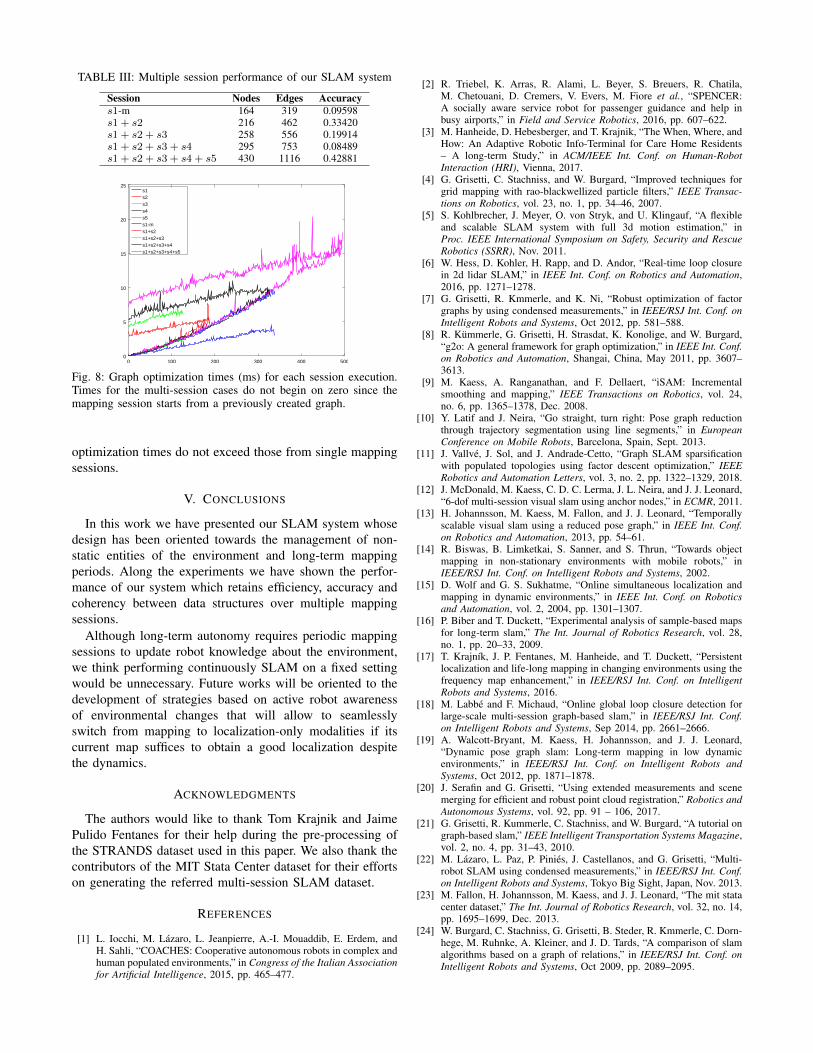
TABLE III: Multiple session performance of our SLAM system

Session Nodes Edges Accuracys1-m 164 319 0.09598s1 + s2 216 462 0.33420s1 + s2 + s3 258 556 0.19914s1 + s2 + s3 + s4 295 753 0.08489s1 + s2 + s3 + s4 + s5 430 1116 0.42881

0 100 200 300 400 5000

5

10

15

20

25s1s2s3s4s5s1-ms1+s2s1+s2+s3s1+s2+s3+s4s1+s2+s3+s4+s5

Fig. 8: Graph optimization times (ms) for each session execution.Times for the multi-session cases do not begin on zero since themapping session starts from a previously created graph.

optimization times do not exceed those from single mappingsessions.

V. CONCLUSIONS

In this work we have presented our SLAM system whosedesign has been oriented towards the management of non-static entities of the environment and long-term mappingperiods. Along the experiments we have shown the perfor-mance of our system which retains efficiency, accuracy andcoherency between data structures over multiple mappingsessions.

Although long-term autonomy requires periodic mappingsessions to update robot knowledge about the environment,we think performing continuously SLAM on a fixed settingwould be unnecessary. Future works will be oriented to thedevelopment of strategies based on active robot awarenessof environmental changes that will allow to seamlesslyswitch from mapping to localization-only modalities if itscurrent map suffices to obtain a good localization despitethe dynamics.

ACKNOWLEDGMENTS

The authors would like to thank Tom Krajnik and JaimePulido Fentanes for their help during the pre-processing ofthe STRANDS dataset used in this paper. We also thank thecontributors of the MIT Stata Center dataset for their effortson generating the referred multi-session SLAM dataset.

REFERENCES

[1] L. Iocchi, M. Lazaro, L. Jeanpierre, A.-I. Mouaddib, E. Erdem, andH. Sahli, “COACHES: Cooperative autonomous robots in complex andhuman populated environments,” in Congress of the Italian Associationfor Artificial Intelligence, 2015, pp. 465–477.

[2] R. Triebel, K. Arras, R. Alami, L. Beyer, S. Breuers, R. Chatila,M. Chetouani, D. Cremers, V. Evers, M. Fiore et al., “SPENCER:A socially aware service robot for passenger guidance and help inbusy airports,” in Field and Service Robotics, 2016, pp. 607–622.

[3] M. Hanheide, D. Hebesberger, and T. Krajnik, “The When, Where, andHow: An Adaptive Robotic Info-Terminal for Care Home Residents– A long-term Study,” in ACM/IEEE Int. Conf. on Human-RobotInteraction (HRI), Vienna, 2017.

[4] G. Grisetti, C. Stachniss, and W. Burgard, “Improved techniques forgrid mapping with rao-blackwellized particle filters,” IEEE Transac-tions on Robotics, vol. 23, no. 1, pp. 34–46, 2007.

[5] S. Kohlbrecher, J. Meyer, O. von Stryk, and U. Klingauf, “A flexibleand scalable SLAM system with full 3d motion estimation,” inProc. IEEE International Symposium on Safety, Security and RescueRobotics (SSRR), Nov. 2011.

[6] W. Hess, D. Kohler, H. Rapp, and D. Andor, “Real-time loop closurein 2d lidar SLAM,” in IEEE Int. Conf. on Robotics and Automation,2016, pp. 1271–1278.

[7] G. Grisetti, R. Kmmerle, and K. Ni, “Robust optimization of factorgraphs by using condensed measurements,” in IEEE/RSJ Int. Conf. onIntelligent Robots and Systems, Oct 2012, pp. 581–588.

[8] R. Kummerle, G. Grisetti, H. Strasdat, K. Konolige, and W. Burgard,“g2o: A general framework for graph optimization,” in IEEE Int. Conf.on Robotics and Automation, Shangai, China, May 2011, pp. 3607–3613.

[9] M. Kaess, A. Ranganathan, and F. Dellaert, “iSAM: Incrementalsmoothing and mapping,” IEEE Transactions on Robotics, vol. 24,no. 6, pp. 1365–1378, Dec. 2008.

[10] Y. Latif and J. Neira, “Go straight, turn right: Pose graph reductionthrough trajectory segmentation using line segments,” in EuropeanConference on Mobile Robots, Barcelona, Spain, Sept. 2013.

[11] J. Vallve, J. Sol, and J. Andrade-Cetto, “Graph SLAM sparsificationwith populated topologies using factor descent optimization,” IEEERobotics and Automation Letters, vol. 3, no. 2, pp. 1322–1329, 2018.

[12] J. McDonald, M. Kaess, C. D. C. Lerma, J. L. Neira, and J. J. Leonard,“6-dof multi-session visual slam using anchor nodes,” in ECMR, 2011.

[13] H. Johannsson, M. Kaess, M. Fallon, and J. J. Leonard, “Temporallyscalable visual slam using a reduced pose graph,” in IEEE Int. Conf.on Robotics and Automation, 2013, pp. 54–61.

[14] R. Biswas, B. Limketkai, S. Sanner, and S. Thrun, “Towards objectmapping in non-stationary environments with mobile robots,” inIEEE/RSJ Int. Conf. on Intelligent Robots and Systems, 2002.

[15] D. Wolf and G. S. Sukhatme, “Online simultaneous localization andmapping in dynamic environments,” in IEEE Int. Conf. on Roboticsand Automation, vol. 2, 2004, pp. 1301–1307.

[16] P. Biber and T. Duckett, “Experimental analysis of sample-based mapsfor long-term slam,” The Int. Journal of Robotics Research, vol. 28,no. 1, pp. 20–33, 2009.

[17] T. Krajnık, J. P. Fentanes, M. Hanheide, and T. Duckett, “Persistentlocalization and life-long mapping in changing environments using thefrequency map enhancement,” in IEEE/RSJ Int. Conf. on IntelligentRobots and Systems, 2016.

[18] M. Labbe and F. Michaud, “Online global loop closure detection forlarge-scale multi-session graph-based slam,” in IEEE/RSJ Int. Conf.on Intelligent Robots and Systems, Sep 2014, pp. 2661–2666.

[19] A. Walcott-Bryant, M. Kaess, H. Johannsson, and J. J. Leonard,“Dynamic pose graph slam: Long-term mapping in low dynamicenvironments,” in IEEE/RSJ Int. Conf. on Intelligent Robots andSystems, Oct 2012, pp. 1871–1878.

[20] J. Serafin and G. Grisetti, “Using extended measurements and scenemerging for efficient and robust point cloud registration,” Robotics andAutonomous Systems, vol. 92, pp. 91 – 106, 2017.

[21] G. Grisetti, R. Kummerle, C. Stachniss, and W. Burgard, “A tutorial ongraph-based slam,” IEEE Intelligent Transportation Systems Magazine,vol. 2, no. 4, pp. 31–43, 2010.

[22] M. Lazaro, L. Paz, P. Pinies, J. Castellanos, and G. Grisetti, “Multi-robot SLAM using condensed measurements,” in IEEE/RSJ Int. Conf.on Intelligent Robots and Systems, Tokyo Big Sight, Japan, Nov. 2013.

[23] M. Fallon, H. Johannsson, M. Kaess, and J. J. Leonard, “The mit statacenter dataset,” The Int. Journal of Robotics Research, vol. 32, no. 14,pp. 1695–1699, Dec. 2013.

[24] W. Burgard, C. Stachniss, G. Grisetti, B. Steder, R. Kmmerle, C. Dorn-hege, M. Ruhnke, A. Kleiner, and J. D. Tards, “A comparison of slamalgorithms based on a graph of relations,” in IEEE/RSJ Int. Conf. onIntelligent Robots and Systems, Oct 2009, pp. 2089–2095.

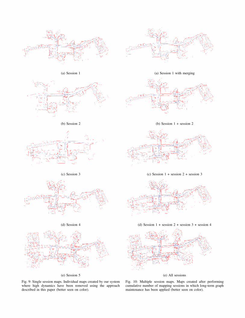
(a) Session 1

(b) Session 2

(c) Session 3

(d) Session 4

(e) Session 5

Fig. 9: Single session maps. Individual maps created by our systemwhere high dynamics have been removed using the approachdescribed in this paper (better seen on color).

(a) Session 1 with merging

(b) Session 1 + session 2

(c) Session 1 + session 2 + session 3

(d) Session 1 + session 2 + session 3 + session 4

(e) All sessions

Fig. 10: Multiple session maps. Maps created after performingcumulative number of mapping sessions in which long-term graphmaintenance has been applied (better seen on color).