Economics Department Discussion Papers Series

ORE Open Research Exeter

TITLE

Production efficiency and constraints on profit taxation and profit distribution in economies withRamsey taxation

AUTHORS

Murty, Sushama

JOURNAL

Social Choice and Welfare

DEPOSITED IN ORE

12 March 2013

This version available at

http://hdl.handle.net/10036/4464

COPYRIGHT AND REUSE

Open Research Exeter makes this work available in accordance with publisher policies.

A NOTE ON VERSIONS

The version presented here may differ from the published version. If citing, you are advised to consult the published version for pagination, volume/issue and date ofpublication

http://hdl.handle.net/10036/4464

Economics Department

Discussion Papers Series ISSN 1473 – 3307

Constraints on profit income distribution and

production efficiency in private ownership economies with Ramsey taxation

Sushama Murty

Paper number 10/10

URL: http://business-school.exeter.ac.uk/economics/papers/

Production Efficiency and Private Shares September 26, 2010

Constraints on profit income distribution and

production efficiency in private ownership economies

with Ramsey taxation∗

Sushama Murty∗

September 2010

∗Department of economics, University of Exeter: [email protected]

Acknowledgement: The basis of this paper is a series of discussions with Charles Blackorby

which led to the identification of some important cases of a more general result which this

paper formalizes and proves. I am very grateful to Charles Blackorby for these discussions

which made it possible for me to study this problem and to present these results.

September 26, 2010


Abstract

In economies with Ramsey taxation, decreasing returns to scale, and private ownership,

we show that second-best production efficiency is desirable when profit tax rates vary

across groups of firms provided that the institutional rules which define profit incomes of

consumers depend on the distribution of profits across these groups of firms. The clas-

sic results of Dasgupta and Stiglitz [1972] (of firm-specific profit taxation) and Diamond

and Mirrlees [1971] and Guesnerie [1995] (of uniform one-hundred percent profit taxation)

follow as special cases of our model. Moreover, second-best analysis suggests the desir-

ability of proportionate taxation of inter-firm transactions in the absence of profit taxes.

Alternatively, it recommends profit taxation as a perfect substitute for intermediate-input

taxation. The analysis also suggests that, combined with the knowledge of the distribution

of profit incomes in the economy, profit taxation can promote both efficiency and redis-

tributive objectives of the government.

Journal of economic literature classification number: H21

Keywords: Ramsey taxation, private ownership, profit taxation, production inefficiency,

general equilibrium.


Constraints on profit income distribution and production efficiency

in private ownership economies with Ramsey taxation

1. Introduction.

Diamond and Mirrlees (DM) [1971] revisited the problem first posed by Ramsey [1927]

about alternative policy instruments that can be employed when there are informational

constraints on the implementation of the second-welfare theorem. Using a general equilib-

rium model they showed that, when personalized lump-sum transfers are not available to

the government as redistributive devices, commodity (Ramsey) taxation can be employed

as an alternative, albeit second-best, means of redistribution. They showed that produc-

tion efficiency was desired by the second-best optimal commodity tax system and that

taxation of inter-firm transactions was not required.

The general equilibrium model they employed was one where technologies of firms

exhibited constant returns to scale. Thus, consumers received no profit incomes. An

extension of this model to decreasing returns to scale technologies (see e.g., Guesnerie

[1995] and Weymark [1979]) led to similar results regarding production efficiency when

private firms were subject to one-hundred percent profit taxation with the proceeds going

back to consumers as a uniform lump-sum transfer (also called a demogrant).1

To check the robustness of the result on second-best production efficiency under more

general settings, the DM model was extended to allow consumers to receive profit incomes

in proportion to the shares that they owned in the private firms.2 A series of papers

pioneered by Dasgupta and Stiglitz (DS) [1972] and followed up by Mirrlees [1972], Hahn

[1973], Sadka [1977], and Munk [1980] concluded that, in such models of privately owned

firms, second-best production efficiency continues to be desirable if the government can

implement firm-specific profit taxes. Challenges in the general proof of this result were

brought to light by these papers and, more recently, by Reinhorn [2010].

In general, the ability of the government to implement a firm-specific system of profit

taxation is questionable. More realistic scenarios, one could argue, may be those where

profit tax rates vary only across groups of private firms, i.e., the number of profit tax rates

the government can peg may be smaller than the number of private firms. Further, the

rigid institutional rules by which profit incomes are distributed among consumers may be

more general than the ones considered in the literature cited above. This paper extends

the above results in these directions.

In particular, we show that second-best production efficiency remains desirable when

profit tax rates can vary across groups of firms provided that the institutional rules which

1 For an excellent exposition of these results see Myles [1995].2 As in a Arrow-Debreu private-ownership economy.

1


define profit incomes of consumers depend on the distribution of profits across these groups

of firms. We show that all the previous results on second-best production efficiency follow

as special cases of our result. On one extreme is the DS case, which involves the finest

partition of the set of private firms–each firm-group in this partition comprises of a single

firm and hence the case of firm-specific profit taxation. On the other extreme is the DM and

Guesnerie [1995] case, which involves the coarsest partition of the set of private firms–only

one firm-group that contains all the firms and government implementing a single (uniform)

rate of profit taxation. Then there are cases that lie in between these two extremes.

Our strategy of proof is different from the earlier papers. Production inefficiency at a

tax equilibrium implies that the aggregate supply of the firms is not on the frontier of the

aggregate technology of the economy. With profit maximizing private and public-sector

firms, this implies that the producer price vectors faced by private and public firms in

such a tax equilibrium are not proportional, implying that there are differences in the

marginal rates of technical substitution across these two types of firms. Hence, an increase

in aggregate supply is technically feasible by reallocating production across these firms.

In fact, we show that, at such a tax equilibrium, there are changes in the price vectors

faced by private and public firms which will ensure that an increase in aggregate supply

is consistent with profit maximizing choices of firms at these new prices. Ceteris paribus,

such an increase in aggregate supply implies an increase in the aggregate income in the

economy. The question is can this increased aggregate income be distributed to consumers

in a manner that respects the existing institutional rules of income distribution in the

economy and improves the welfare of all consumers? In general, the institutional rules of

income distribution and the restrictions on the ability of the government to implement

profit taxation can constrain severely such welfare improvements. However, we show that

our institutional set-up that we described above permits the distribution of the increased

aggregate income across consumers in a welfare improving manner.

In our proof, we take recourse to an intermediate construct of an economy with

producer price vectors varying across (groups of) private-sector firms.3 Hence, implicitly,

this implies a wedge between price vectors faced by firms and, hence, the taxation of

transactions between firms are allowed. We show that this economy exhibits second-best

production efficiency, albeit, unlike in the DM model, this means that firms are subject

to proportionate rates of intermediate-input taxation. It is shown that the second-best

allocations of this economy are the same as those of an economy where all private firms

face the same price vector but are subject to profit taxes. This implies that second-

best equilibrium allocations with intermediate-input taxation can also be decentralized as

3 This is as in the earlier literature.

2


second-best tax equilibrium allocations with no intermediate-input taxation but with firms

being subject to profit taxation.

The results on second-best production efficiency and intermediate-input taxation are

important for three reasons: Second-best production efficiency supports the use of pro-

ducer prices as the right proxies for the generally unobservable shadow prices for the cost-

benefit evaluation of public sector projects.4 The recommendation of either proportionate

intermediate-goods taxation or profit taxation with no intermediate-goods taxation min-

imizes also the practical administrative costs of implementing a system of Ramsey taxes,

e.g., it supports tax structures like VAT. Our analysis also suggests how, by understand-

ing the rules of profit income distribution in the economy, the government can potentially

design a system of profit taxation that can further both its redistributive and efficiency

objectives.

In Section 2, we lay out our general equilibrium model. We define two types of profit-

making economies–those with firm-group specific profit taxes and those with firm group

specific prices. In Section 3 we prove a preliminary lemma. In Section 4, we employ this

lemma to prove Theorem 1 that states that second-best production efficiency is desirable

in profit-making economies with firm-group specific prices. In Section 5, we obtain as

corollaries of Theorem 1 two results: one, the desirability of second-best production effi-

ciency in profit-making economies with firm-group specific profit taxes and two, the case

for either proportionate intermediate-input taxation in profit-making economies or profit

taxation with no intermediate goods taxation. In Section 6, we conclude.

2. The model.

There are N commodities indexed by k, H consumers indexed by h, and I + 1 firms

indexed by i. We denote the index set of consumers as H = {1, . . . , H} and the index set

of firms as I = {0, . . . , I}. We assume that firm 0 is a public sector firm, while all others

are private firms.

For every firm i ∈ I, the technology is denoted by Y i ⊂ RN . The aggregate technol-

ogy is Y =∑

i Yi.

For all h ∈ H, the gross consumption set of consumer h is Xh ⊆ RN+ and the

preferences over Xh are represented by continuous, quasi-concave, and locally nonsatiated

utility functions uh : Xh → R with images uh(xh). The endowment vector of consumer h

is denoted by eh ∈ RN+ .

Let E = ((Xh, uh, eh)h∈H, (Y i)i∈I) denote the vector of economic fundamentals spec-

ified above.

4 See Little and Mirrlees [1974], Boadway [1975], and Dreze and Stern [1987].

3


We assume that all firms are price-takers. For all i ∈ I define the set of prices for

which profit maximization is well defined as

Bi := {p ∈ RN+ \ {0N}| p · y is bounded from above for all y ∈ Y i} (2.1)

and define the profit function πi : Bi → R with image

πi(p) = supyi

{p · yi| yi ∈ Y i}. (2.2)

The supply vectors of firm i ∈ I are obtained from the solution mapping of (2.2) as

yi : Bi → RN with image yi(p).5 For all i ∈ I define the frontier of Y i as

Y i = {yi ∈ Y i| yi ≥ yi implies that yi /∈ Y i}. (2.3)

Similarly, we can define Y as the frontier of the aggregate technology Y .

The vector of consumer prices is denoted by q ∈ RN+ . Income of every consumer h ∈ H

is denoted by mh ∈ R+. Let the mapping xh : RN+ × R+ → RN with image xh(q, mh)

denote the Marshallian demand vector of consumer h and let the mapping V h : RN+×R+ →

R with image V h(q, mh) be the corresponding indirect utility function. Every consumer

receives a demogrant, which is denoted by m ∈ R. The income of consumer h ∈ H in

economy E comprises of his endowment income, profit income that he receives from the

private firms, and the demogrant that he receives from the government. A partition of

I \{0} (the index set of all private sector firms) is denoted by P = {P1, . . . , PT}. Members

of a partition will be indexed by t or l.

2.1. A profit-making economy with firm-group specific profit taxes.

A profit-making economy with firm-group specific profit taxes is an economy derived

from E where the private firms are partitioned into various groups, the government can

implement profit taxation with the profit tax rates varying across firms depending on the

groups to which they belong, and the consumers receive profit incomes which depend on

the distribution of firm-group profits. If P = {P1, . . . , PT} is such a partition, then we

denote the vector of firm-group specific profit tax rates by τ = 〈τ1, . . . , τT 〉 ∈ RT , i.e., all

firms in each firm-group t = 1, . . . , T are subject to the same profit tax rate τ t so that the

net of tax profit of firm-group t is (1 − τ t)∑

i∈Ptπi(p), which we denote in the definition

below by the function at. The profit incomes that consumers receive in such economies

assume the form below. The form is very general requiring only that profit incomes of

all consumers should add up to the total net of tax profits in the economy (condition (i)

in the definition below) and that the profit income received by each consumer should be

5 In general, yi(p) need not be a singleton set, i.e., the solution mapping yi(p) need not be a function.

4


non-negative (condition (ii) in the definition below). Examples 1 to 3 below consider a

well-known functional form and some of its special cases that satisfy these conditions.

Definition. A map of profit incomes with firm-group specific profit taxes that is associated

with a partition P = {P1, . . . , PT} of I \ {0} is a continuous vector-valued map

rP,τ : RT −→ RH (2.4)

with image

r1 = r1P,τ ( a1, . . . , aT )

...rH = rH

P,τ ( a1, . . . , aT )

, (2.5)

where a = 〈a1, . . . , aT 〉 is obtained as the vector-valued mapping a : RT ×∩i∈I\{0}Bi −→

RT with image

a1(τ1, . . . , τT , p) = (1 − τ1)∑

i∈P1πi(p)

...aT (τ1, . . . , τT , p) = (1 − τT )

∑

i∈PTπi(p)

(2.6)

such that

(i)∑

h∈H rhP,τ

(

(1−τ1)∑

i∈P1πi(p) , . . . , (1−τT )

∑

i∈PTπi(p)

)

=∑

Pt∈P(1−τ t)

∑

i∈Ptπi(p)

and

(ii) for all h ∈ H, rhP,τ

(

(1 − τ1)∑

i∈P1πi(p) , . . . , (1 − τT )

∑

i∈PTπi(p)

)

≥ 0.

Definition. Let E(E,P , rP,τ ) denote a profit-making economy with firm-group specific

profit taxes associated with a partition P = {P1, . . . , PT} of I \ {0} and a map of profit

incomes rP,τ . A tax equilibrium of E(E,P , rP,τ ) is a configuration 〈q, p, p0, τ1, . . . , τT , m〉 ∈

R3N+ × RT+1 such that6

∑

h∈H

xh(q, mh) ≤T

∑

t=1

∑

i∈Pt

yi((1 − τ t)p) + y0(p0) +∑

h∈H

eh and

mh = rhP,τ ((1 − τ1)

∑

i∈P1

πi(p), . . . , (1 − τT )∑

i∈PT

πi(p)) + m + qeh, ∀ h ∈ H.

(2.8)

6 Vector notation: for x and y in Rn,

x ≥ y ⇔ xi ≥ yi, ∀i = 1, . . . , n,

x > y ⇔ x 6= y and xi ≥ yi, ∀i = 1, . . . , n,

x ≫ y ⇔ xi > yi, ∀i = 1, . . . , n.

(2.7)

Also, recall that the income mh of each consumer h comprises of his profit income, endowment income,and the demogrant received from the government.

5


Some examples.

Consider the standard case where the profits are distributed to consumers according

to an exogeneous H×I-dimensional matrix of shares Θ with typical element θhi ≥ 0 which

denotes the share of consumer h in the profit of the private firm i. Thus, we require∑

h θhi = 1 for all i ∈ I and h ∈ H. Let O denote the set of matrices Θ with these

properties.

Example 1. Let Θ ∈ O. If P ={

{1}, . . . , {I}}

(i.e., P is the finest partition of the set of

all private firms), then the map of profit incomes with firm-group specific profit taxes is

given by

rh = rhP,p((1−τ1)π1(p), . . . , (1−τ I)πI(p)) = θh

1 (1−τ1)π1(p)+. . .+θhI (1−τ I)πI(p), ∀ h ∈ H.

(2.9)

This is the DS case of firm-specific profit taxation.

Example 2. If Θ ∈ O is such that θhi = θh for all h ∈ H and i ∈ I \ {0}, then the coarsest

partition P of I \ {0} that can be used to define a map of profit incomes with firm-group

specific profit taxes is P = {I \ {0}} and the map of profit incomes is given by

rh = rhP,p((1 − τ)

∑

i∈I\{0}

πi(p)) = θh(1 − τ)∑

i∈I

πi(p), ∀ h ∈ H. (2.10)

A special case of this example is θh = 1

Hand τ = 0. This is equivalent to the Guesnerie

[1995] and Weymark [1979] case, where the profits of all firms are subject to a uniform

(one-hundred percent) profit tax rate and the government returns its profit tax revenue as

a uniform lump-sum transfer to all consumers.7

Example 3. P = {P1, . . . , PT}. Let Θ ∈ O be such that θhi = θht for all h ∈ H, t = 1, . . . , T ,

and i ∈ Pt. Then, the map of profit incomes with firm-group specific profit taxes is given

by

rh = rhP,p(

∑

i∈P1

(1 − τ1)πi(p), . . . ,∑

i∈PT

(1 − τT )πi(p))

= θh1(1 − τ1)∑

i∈P1

πi(p) + . . . + θhT (1 − τT )∑

i∈PT

πi(p), ∀ h ∈ H.(2.11)

This covers the case where government can implement more than a single but not quite

firm-specific profit tax rates, i.e., 0 < T < I, and where profit incomes of consumers

depend on distribution of profits in the T groups of firms.

7 This is also trivially the DM case where constant returns to scale is assumed, so that profits of firmsare zero.

6


Definition. Let E(E,P , rP,τ ) be a profit-making economy with firm-group specific profit

taxes associated with a partition P = 〈P1, . . . , PT 〉 of I \ {0} and a map of profit incomes

rP,τ . A tax equilibrium 〈q, p, p0, τ1, . . . , τT , m〉 of E(E,P , rP,τ ) is a production efficient

tax equilibrium of E(E,P , rP,τ ) if∑I

i=1yi(p) + y0(p0) ∈ Y .

The second-best problem for E(E,P , rP,τ ) is to find the mapping VP,rP,τ: ∆H−1 → R

with image8

VP,rP,τ(s1, . . . , sH) := max

q, p, p0, 〈τ1,...,τT 〉, m

∑

h

shV h(q, mh)

subject to

〈q, p, p0, τ1, . . . , τT , m〉 satisfying (2.8).

(2.12)

A solution to (2.12) is called a second-best tax equilibrium of E(E,P , rP,τ ).

Definition. A second-best tax equilibrium 〈∗q , ∗p, ∗p0, ∗τ 1, . . . , ∗τT , ∗m〉 of E(E,P , rP,τ ) is a

production efficient second-best if it is production efficient. If all second-best tax equilibria

of E(E,P , rP,τ ) are production efficient, then E(E,P , rP,τ ) exhibits second-best production

efficiency or production efficiency is desirable at the second-best of E(E,P , rP,τ ).

2.2. A profit-making economy with firm-group specific prices.

In this paper, we show that production efficiency is desirable at the second-best of

E(E,P , rP,τ ). To do so, we consider a more general institutional structure than a profit-

making economy with firm-group specific profit taxes. This is an economy with profit

incomes where the government can implement firm-group specific prices. We denote such

an economy by E(E,P , rP,p). The set of tax equilibrium allocations of E(E,P , rP,τ ) turns

out to be a subset of the set of tax equilibrium allocations of E(E,P , rP,p). Moreover,

we show in Section 4 that E(E,P , rP,p) exhibits second-best production efficiency. In

Section 5 we show that all the second-best tax equilibrium allocations of E(E,P , rP,p)

can be decentralized as tax equilibrium allocations of E(E,P , rP,τ ). The desirability of

production efficiency at the second-best of E(E,P , rP,τ ) will hence follow.

Let P = {P1, . . . , PT} be a partition of I \ {0}. For all t = 1, . . . , T , we denote

∩i∈PtBi by Bt and the price vector faced by firm-group Pt is denoted by pt ∈ RN

+ .

Definition. A map of profit incomes with firm-group specific prices that is associated with

a partition P = {P1, . . . , PT} of I \ {0} is a continuous vector-valued map

rP,p : RT −→ RH (2.13)

8 ∆H−1 is the H − 1-dimensional unit simplex in RH . 〈s1, . . . , sH〉 ∈ ∆H−1 can be interpreted as

a vector of welfare weights attached to consumer utilities. The second-best utility possibility frontier isobtained by solving the second-best optimization for all possible vectors of welfare weights.

7


with image

r1 = r1P,p( a1, . . . , aT )

...rH = rH

P,p( a1, . . . , aT )

, (2.14)

where a = 〈a1, . . . , aT 〉 is obtained as the vector-valued mapping a :∏T

t=1Bt −→ RT with

image

a1(p1, . . . , pT ) =∑

i∈P1πi(p1)

...aT (p1, . . . , pT ) =

∑

i∈PTπi(pT )

(2.15)

such that

(i)∑

h∈H rhP,p(

∑

i∈P1πi(p1) , . . . ,

∑

i∈PTπi(pT )) =

∑

Pt∈P

∑

i∈Ptπi(pt) and

(ii) for all h ∈ H, rhP,p(

∑

i∈P1πi(p1) , . . . ,

∑

i∈PTπi(pT )) ≥ 0.

Definition. Let E(E,P , rP,p) denote a profit-making economy with firm-group specific

prices associated with a partition P = {P1, . . . , PT} of I \ {0} and a map of profit

incomes rP,p. A tax equilibrium of E(E,P , rP,p) is a configuration 〈q, p1, . . . , pT , m〉 ∈

RN+ ×

∏Tt=1

Bt × R such that

∑

h∈H

xh(q, mh) ≤T

∑

t=1

∑

i∈Pt

yi(pt) + y0(p0) +∑

h∈H

eh and

mh = rhP,p(

∑

i∈P1

πi(p1), . . . ,∑

i∈PT

πi(pT )) + m + qeh, ∀ h ∈ H.

(2.16)

As in the previous section we can define an efficient tax equilibrium of economy

E(E,P , rP,p). Note that the system of equations (2.16) is homogeneous of degree zero in

in p1, . . . , pT , q, and m and is homogeneous of degree zero in p0. Hence, it admits two

normalization rules.9 Under the maintained assumptions on consumers’ preferences, the

budget constraints hold as equalities under utility maximization, that is, for all h, we have

q · xh(q, mh) = mh. (2.17)

To show that at a tax equilibrium of E(E,P , rP,p), the government budget is balanced, we

multiply both sides of the first part (a vector of inequalities) of (2.16) by q and employ

9 For example, we can adopt the normalization rules p11 = 1 and p0

1 = 1.

8


(2.17) to obtain

q ·∑

h

xh(q, mh) ≤ q ·T

∑

t=1

∑

i∈Pt

yi(pt) + q · y0(p0) + q ·∑

h∈H

eh

⇒T

∑

t=1

∑

i∈Pt

πi(pt) + Hm + q ·∑

h∈H

eh ≤

T∑

t=1

∑

i∈Pt

pt · yi(pt) + q · y0(p0) +T

∑

t=1

∑

i∈Pt

[q − pt] · yi(pt) + q ·∑

h∈H

eh

⇒ Hm ≤T

∑

t=1

∑

i∈Pt

[q − pt] · yi(pt) + q · y0(p0)

⇒ m ≤

∑Tt=1

∑

i∈Pt[q − pt] · yi(pt) + q · y0(p0)

H

⇒ m ≤

∑Tt=1

∑

i∈Pt[q − pt] · yi(pt) + [q − p0] · y0(p0) + p0 · y0(p0)

H.

(2.18)

Condition (2.18), which is an implication of Walras law, says that the demogrant is financed

from the government’s revenue from indirect taxation and the sale of publicly produced

goods to the consumers.

The second-best problem for E(E,P , rP,p) is to find the mapping VP,rP,p: ∆H−1 → R

with image

VP,rP,p(s1, . . . , sH) := max

q, p0, 〈p1,...,pT 〉, m

∑

h

shV h(q, mh)

subject to

〈q, p0, p1, . . . , pT , m〉 satisfying (2.16).

(2.19)

A solution to (2.19) is called a second-best tax equilibrium of E(E,P , rP,p). As in the previ-

ous section we can define a production efficient second-best tax equilibrium of E(E,P , rP,p)

and the desirability of production efficiency at the second-best of E(E,P , rP,p).

3. A preliminary lemma.

Assumptions 1 and 2 stated below are regularity assumptions on the technologies of

firms. They are similar to the ones employed in the previous literature on this topic.

Assumption 1. For all i ∈ I, Y i is closed, convex, contains 0, is not a cone, and satisfies

Y i + RN− ⊂ Y i.

9


Assumption 2. For all i ∈ I, the set Bi is non-empty and there exists ρ ∈ RN++ ∩ Bi.

Assumption 1 excludes firms that exhibit constant returns-to-scale. This exclusion

seems without loss of generality as these firms are associated with zero profits and hence

the presence of such firms offers no constraints on the distribution of profits in the economy

(the issue of focus in this paper). Note that under Assumptions 1 and 2, for all i, πi is

continuous, non-negative valued, linearly homogeneous, and convex on the set Bi.

Let E(E,P , rP,p) denote a profit-income economy with firm-group specific prices as-

sociated with a partition P = {P1, . . . , PT} of I \ {0}. For all t = 1, . . . , T and pt ∈ Bt,

we denote the supply of firms in Pt ∈ P as yt(pt), i.e., yt(pt) =∑

i∈Ptyi(pt). For all

t = 1, . . . , T , the frontier of Y t =∑

i∈PtY i is denoted by Y t.10

Let 〈p1, . . . , pT 〉 ∈∏T

t=1Bt and p0 ∈ B0. Assumption 3 (below) restricts our analysis

(which we claim is without loss of generality11) to the case of technologies with smooth

frontiers.

Remark 1 (below) presents the well-known fact that, under our assumptions, the

vector of aggregate supply∑T

t=1yt(pt)+ y0(p0) lies in Y if the price vectors p0, . . . , pT are

proportional.

Lemma 1 shows that if there exist t, t′ ∈ {0, 1, . . . , T} such that pt and pt′ are not

proportional,12 then there exist changes in price vectors faced by firms in groups t and t′

that can strictly increase the aggregate supply (i.e., lead to a higher aggregate supply than∑T

l=1yl(pl) + y0(p0)) given the profit maximizing behavior of our price-taking firms and,

hence,∑T

l=1yl(pl) + y0(p0) is not in Y . Before formally stating Lemma 1, we first present

two examples to illustrate the point made in this lemma. Example 4 (below) considers the

case of smooth production frontiers, while Example 5 shows that the argument extends to

the non-smooth case. In both the examples, it is assumed that N = 2, there is no public

production, I = 2, and P ={

{1}, {2}}

. Good two is the output and good one is the

input of these firms, so that if y = 〈y1, y2〉 ∈ R2 is a production vector, then y2 ≥ 0 and

y1 ≤ 0. Let us also denote a hyperplane with normal p and constant a by H(p, a) and its

lower and strictly lower half-spaces by H≤(p, a) and H<(p, a), respectively. Similarly we

can define the upper and strictly upper half-spaces of H(p, a).

10 Note the slight abuse of notation: the technology, its frontier, and a production vector correspondingto any firm i ∈ I are denoted by Y i, Y i, and yi, respectively, while the aggregate technology, its frontier,and a production vector obtained by summing over all firms in Pt for t = 1, . . . , T are denoted by Y t, Y t,and yt, respectively. However, in what follows, it will be clear always whether we are referring to a firmin I or to a group of firms Pt.11 We defend this claim with an example below.12 Or, in the non-smooth case, if the sets of support prices of yt(pt) and yt′(pt′) do not intersect.

10


Example 4. Suppose technology of Firm 1 is Y 1 = {y1 ∈ R2| y12 ≤ (−y1

1)12} and Y 2 =

{y2 ∈ R2| y22 ≤ (−y2

1)13}. Suppose Firms 1 and 2 face price vectors p1 = 〈1, 1

2〉 and

p2 = 〈1, 1

12〉, respectively. It can be verified that the profit maximizing production vector

of Firm 1 will be y1(p1) = 〈−1, 1〉, while that of Firm 2 will be y2(p2) = 〈−8, 2〉. Since p1

and p2 are not proportional, it is well-known (and can be easily verified) that the aggregate

production vector y := y1(p1) + y2(p2) = 〈−9, 3〉 must lie in the interior of Y := Y 1 + Y 2.

In fact, at these production vectors, the marginal productivity of input in Firm 1 is 2,

which is less than the marginal productivity of input equal to 12 in Firm 2. This suggests

that reallocating some of the input from Firm 1 to Firm 2 will result in an increase in the

aggregate output. The question is whether there exist such reallocations which can also

be supported as profit maximization choices of firms. We show below that this is true.

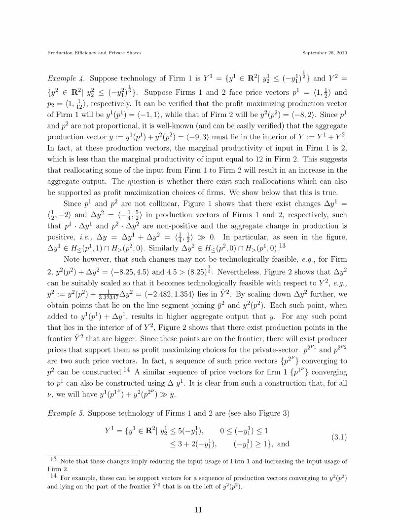
Since p1 and p2 are not collinear, Figure 1 shows that there exist changes ∆y1 =

〈1

2,−2〉 and ∆y2 = 〈−1

4, 5

2〉 in production vectors of Firms 1 and 2, respectively, such

that p1 · ∆y1 and p2 · ∆y2 are non-positive and the aggregate change in production is

positive, i.e., ∆y = ∆y1 + ∆y2 = 〈1

4, 1

2〉 ≫ 0. In particular, as seen in the figure,

∆y1 ∈ H≤(p1, 1) ∩ H>(p2, 0). Similarly ∆y2 ∈ H≤(p2, 0) ∩ H>(p1, 0).13

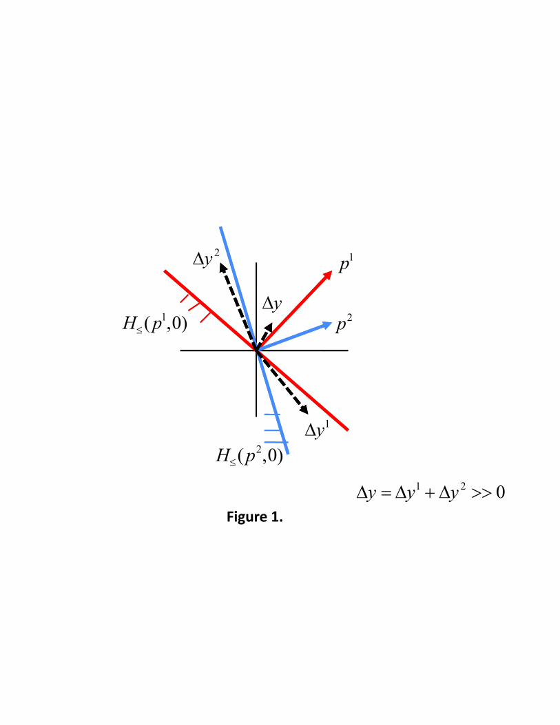
Note however, that such changes may not be technologically feasible, e.g., for Firm

2, y2(p2) + ∆y2 = 〈−8.25, 4.5〉 and 4.5 > (8.25)13 . Nevertheless, Figure 2 shows that ∆y2

can be suitably scaled so that it becomes technologically feasible with respect to Y 2, e.g.,

y2 := y2(p2) + 1

3.32347∆y2 = 〈−2.482, 1.354〉 lies in Y 2. By scaling down ∆y2 further, we

obtain points that lie on the line segment joining y2 and y2(p2). Each such point, when

added to y1(p1) + ∆y1, results in higher aggregate output that y. For any such point

that lies in the interior of of Y 2, Figure 2 shows that there exist production points in the

frontier Y 2 that are bigger. Since these points are on the frontier, there will exist producer

prices that support them as profit maximizing choices for the private-sector. p2ν1 and p2ν2

are two such price vectors. In fact, a sequence of such price vectors {p2ν} converging to

p2 can be constructed.14 A similar sequence of price vectors for firm 1 {p1ν} converging

to p1 can also be constructed using ∆ y1. It is clear from such a construction that, for all

ν, we will have y1(p1ν) + y2(p2ν

) ≫ y.

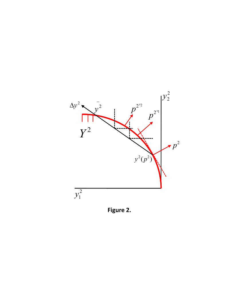
Example 5. Suppose technology of Firms 1 and 2 are (see also Figure 3)

Y 1 = {y1 ∈ R2| y12 ≤ 5(−y1

1), 0 ≤ (−y11) ≤ 1

≤ 3 + 2(−y11), (−y1

1) ≥ 1}, and(3.1)

13 Note that these changes imply reducing the input usage of Firm 1 and increasing the input usage ofFirm 2.14 For example, these can be support vectors for a sequence of production vectors converging to y2(p2)

and lying on the part of the frontier Y 2 that is on the left of y2(p2).

11

H!(p2,0)

H!(p1,0) p

2

p1

"y1

"y 2

"y # "y1 $ "y 2 %% 0

"y

Figure 1.

"y 2y2&

y2(p2)

p2

p2v1

Y2

p2v2

Figure 2.

y12

y22

y1&

y2&

p1 p

2

'1(y1)

'2(y 2)

y2

y1~

p1

Y1

Y2

y11

y21

y22

y12

Figure 3.

y1

! ()

##

)()(

,

2211

1~22

~2

yy

ppyy

''

p1


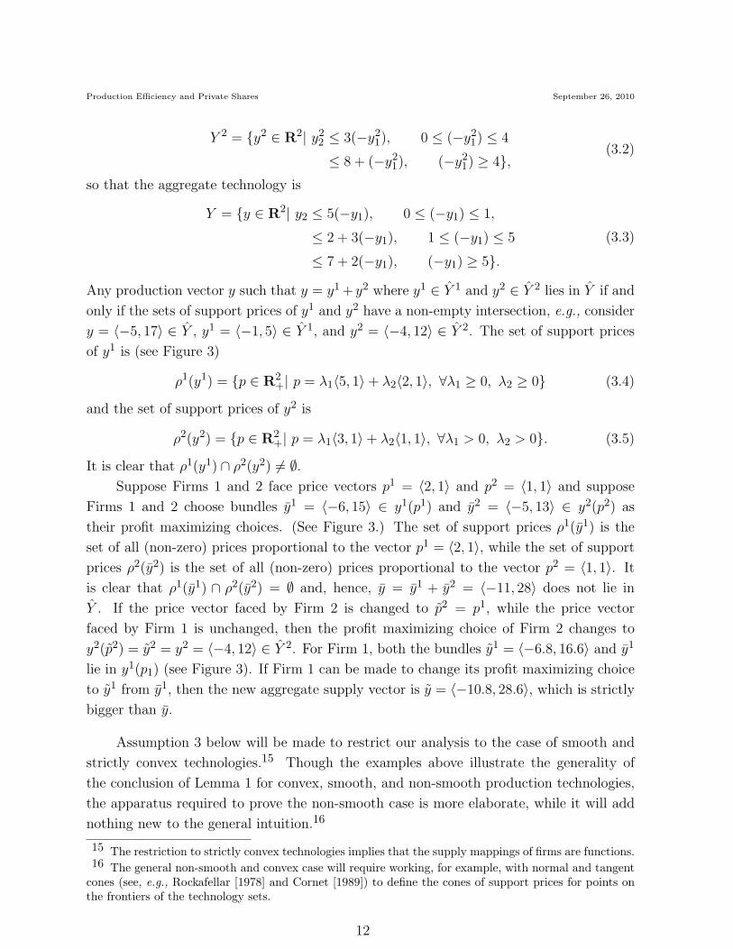
Y 2 = {y2 ∈ R2| y22 ≤ 3(−y2

1), 0 ≤ (−y21) ≤ 4

≤ 8 + (−y21), (−y2

1) ≥ 4},(3.2)

so that the aggregate technology is

Y = {y ∈ R2| y2 ≤ 5(−y1), 0 ≤ (−y1) ≤ 1,

≤ 2 + 3(−y1), 1 ≤ (−y1) ≤ 5

≤ 7 + 2(−y1), (−y1) ≥ 5}.

(3.3)

Any production vector y such that y = y1 +y2 where y1 ∈ Y 1 and y2 ∈ Y 2 lies in Y if and

only if the sets of support prices of y1 and y2 have a non-empty intersection, e.g., consider

y = 〈−5, 17〉 ∈ Y , y1 = 〈−1, 5〉 ∈ Y 1, and y2 = 〈−4, 12〉 ∈ Y 2. The set of support prices

of y1 is (see Figure 3)

ρ1(y1) = {p ∈ R2+| p = λ1〈5, 1〉 + λ2〈2, 1〉, ∀λ1 ≥ 0, λ2 ≥ 0} (3.4)

and the set of support prices of y2 is

ρ2(y2) = {p ∈ R2+| p = λ1〈3, 1〉 + λ2〈1, 1〉, ∀λ1 > 0, λ2 > 0}. (3.5)

It is clear that ρ1(y1) ∩ ρ2(y2) 6= ∅.

Suppose Firms 1 and 2 face price vectors p1 = 〈2, 1〉 and p2 = 〈1, 1〉 and suppose

Firms 1 and 2 choose bundles y1 = 〈−6, 15〉 ∈ y1(p1) and y2 = 〈−5, 13〉 ∈ y2(p2) as

their profit maximizing choices. (See Figure 3.) The set of support prices ρ1(y1) is the

set of all (non-zero) prices proportional to the vector p1 = 〈2, 1〉, while the set of support

prices ρ2(y2) is the set of all (non-zero) prices proportional to the vector p2 = 〈1, 1〉. It

is clear that ρ1(y1) ∩ ρ2(y2) = ∅ and, hence, y = y1 + y2 = 〈−11, 28〉 does not lie in

Y . If the price vector faced by Firm 2 is changed to p2 = p1, while the price vector

faced by Firm 1 is unchanged, then the profit maximizing choice of Firm 2 changes to

y2(p2) = y2 = y2 = 〈−4, 12〉 ∈ Y 2. For Firm 1, both the bundles y1 = 〈−6.8, 16.6〉 and y1

lie in y1(p1) (see Figure 3). If Firm 1 can be made to change its profit maximizing choice

to y1 from y1, then the new aggregate supply vector is y = 〈−10.8, 28.6〉, which is strictly

bigger than y.

Assumption 3 below will be made to restrict our analysis to the case of smooth and

strictly convex technologies.15 Though the examples above illustrate the generality of

the conclusion of Lemma 1 for convex, smooth, and non-smooth production technologies,

the apparatus required to prove the non-smooth case is more elaborate, while it will add

nothing new to the general intuition.16

15 The restriction to strictly convex technologies implies that the supply mappings of firms are functions.16 The general non-smooth and convex case will require working, for example, with normal and tangent

cones (see, e.g., Rockafellar [1978] and Cornet [1989]) to define the cones of support prices for points onthe frontiers of the technology sets.

12


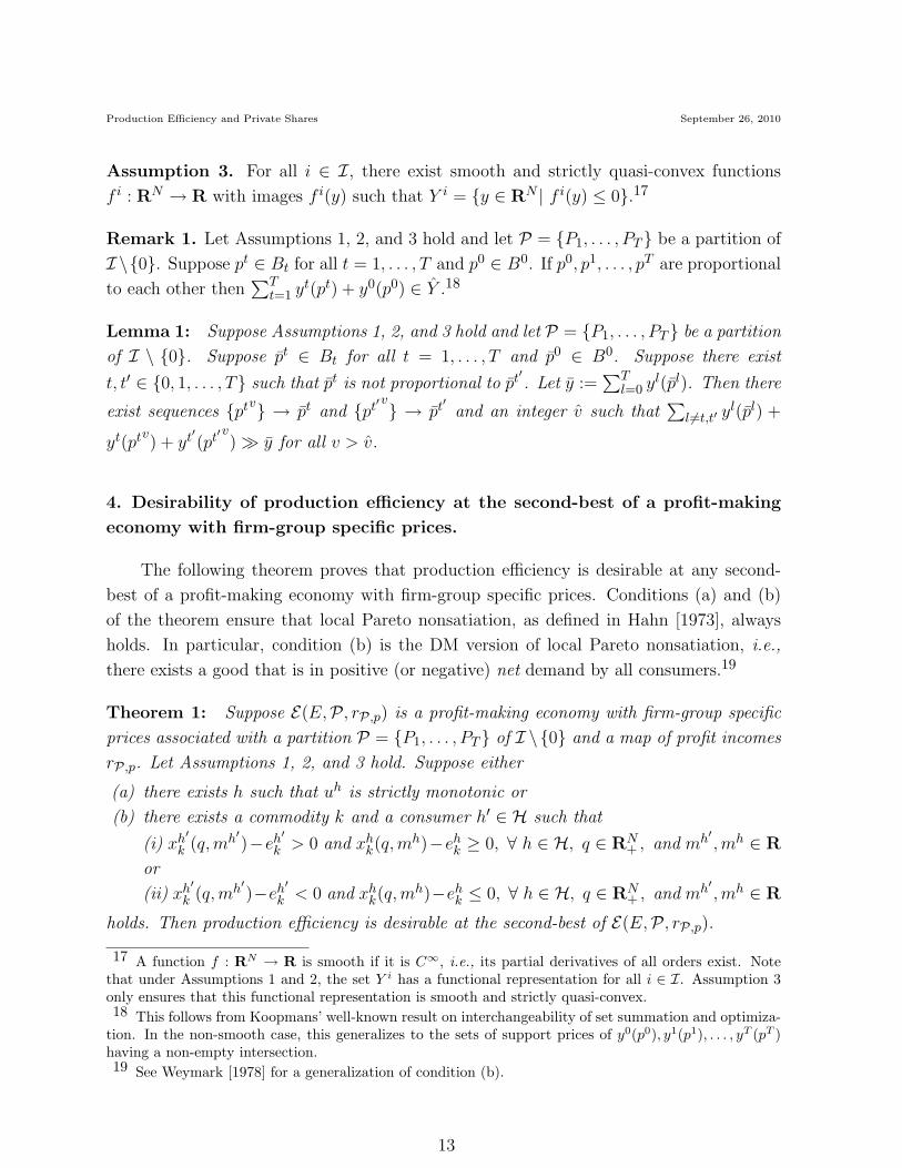
Assumption 3. For all i ∈ I, there exist smooth and strictly quasi-convex functions

f i : RN → R with images f i(y) such that Y i = {y ∈ RN | f i(y) ≤ 0}.17

Remark 1. Let Assumptions 1, 2, and 3 hold and let P = {P1, . . . , PT} be a partition of

I \{0}. Suppose pt ∈ Bt for all t = 1, . . . , T and p0 ∈ B0. If p0, p1, . . . , pT are proportional

to each other then∑T

t=1yt(pt) + y0(p0) ∈ Y .18

Lemma 1: Suppose Assumptions 1, 2, and 3 hold and let P = {P1, . . . , PT} be a partition

of I \ {0}. Suppose pt ∈ Bt for all t = 1, . . . , T and p0 ∈ B0. Suppose there exist

t, t′ ∈ {0, 1, . . . , T} such that pt is not proportional to pt′. Let y :=∑T

l=0yl(pl). Then there

exist sequences {ptv} → pt and {pt′v} → pt′ and an integer v such that

∑

l 6=t,t′ yl(pl) +

yt(ptv) + yt′(pt′v) ≫ y for all v > v.

4. Desirability of production efficiency at the second-best of a profit-making

economy with firm-group specific prices.

The following theorem proves that production efficiency is desirable at any second-

best of a profit-making economy with firm-group specific prices. Conditions (a) and (b)

of the theorem ensure that local Pareto nonsatiation, as defined in Hahn [1973], always

holds. In particular, condition (b) is the DM version of local Pareto nonsatiation, i.e.,

there exists a good that is in positive (or negative) net demand by all consumers.19

Theorem 1: Suppose E(E,P , rP,p) is a profit-making economy with firm-group specific

prices associated with a partition P = {P1, . . . , PT} of I \{0} and a map of profit incomes

rP,p. Let Assumptions 1, 2, and 3 hold. Suppose either

(a) there exists h such that uh is strictly monotonic or

(b) there exists a commodity k and a consumer h′ ∈ H such that

(i) xh′

k (q, mh′

)−eh′

k > 0 and xhk(q, mh)−eh

k ≥ 0, ∀ h ∈ H, q ∈ RN+ , and mh′

, mh ∈ R

or

(ii) xh′

k (q, mh′

)−eh′

k < 0 and xhk(q, mh)−eh

k ≤ 0, ∀ h ∈ H, q ∈ RN+ , and mh′

, mh ∈ R

holds. Then production efficiency is desirable at the second-best of E(E,P , rP,p).

17 A function f : RN → R is smooth if it is C∞, i.e., its partial derivatives of all orders exist. Note

that under Assumptions 1 and 2, the set Y i has a functional representation for all i ∈ I. Assumption 3only ensures that this functional representation is smooth and strictly quasi-convex.18 This follows from Koopmans’ well-known result on interchangeability of set summation and optimiza-

tion. In the non-smooth case, this generalizes to the sets of support prices of y0(p0), y1(p1), . . . , yT (pT )having a non-empty intersection.19 See Weymark [1978] for a generalization of condition (b).

13


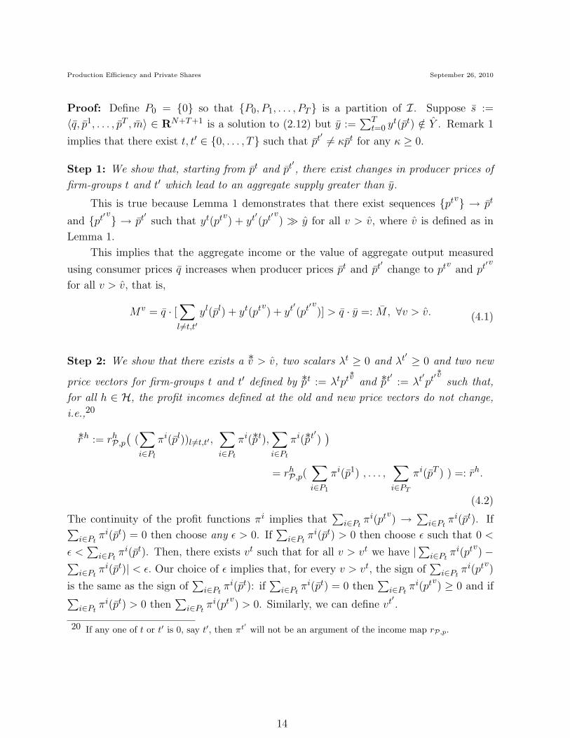
Proof: Define P0 = {0} so that {P0, P1, . . . , PT} is a partition of I. Suppose s :=

〈q, p1, . . . , pT , m〉 ∈ RN+T+1 is a solution to (2.12) but y :=∑T

t=0yt(pt) /∈ Y . Remark 1

implies that there exist t, t′ ∈ {0, . . . , T} such that pt′ 6= κpt for any κ ≥ 0.

Step 1: We show that, starting from pt and pt′, there exist changes in producer prices of

firm-groups t and t′ which lead to an aggregate supply greater than y.

This is true because Lemma 1 demonstrates that there exist sequences {ptv} → pt

and {pt′v} → pt′ such that yt(ptv) + yt′(pt′

v) ≫ y for all v > v, where v is defined as in

Lemma 1.

This implies that the aggregate income or the value of aggregate output measured

using consumer prices q increases when producer prices pt and pt′ change to ptv and pt′v

for all v > v, that is,

Mv = q · [∑

l 6=t,t′

yl(pl) + yt(ptv) + yt′(pt′v)] > q · y =: M, ∀v > v. (4.1)

Step 2: We show that there exists a ∗v > v, two scalars λt ≥ 0 and λt′ ≥ 0 and two new

price vectors for firm-groups t and t′ defined by ∗pt := λtpt∗v

and ∗pt′ := λt′pt′∗v

such that,

for all h ∈ H, the profit incomes defined at the old and new price vectors do not change,

i.e.,20

∗rh := rhP,p

(

(∑

i∈Pl

πi(pl))l 6=t,t′ ,∑

i∈Pt

πi(∗pt),∑

i∈Pt

πi(∗pt′))

= rhP,p(

∑

i∈P1

πi(p1) , . . . ,∑

i∈PT

πi(pT ) ) =: rh.

(4.2)

The continuity of the profit functions πi implies that∑

i∈Ptπi(ptv) →

∑

i∈Ptπi(pt). If

∑

i∈Ptπi(pt) = 0 then choose any ǫ > 0. If

∑

i∈Ptπi(pt) > 0 then choose ǫ such that 0 <

ǫ <∑

i∈Ptπi(pt). Then, there exists vt such that for all v > vt we have |

∑

i∈Ptπi(ptv) −

∑

i∈Ptπi(pt)| < ǫ. Our choice of ǫ implies that, for every v > vt, the sign of

∑

i∈Ptπi(ptv)

is the same as the sign of∑

i∈Ptπi(pt): if

∑

i∈Ptπi(pt) = 0 then

∑

i∈Ptπi(ptv) ≥ 0 and if

∑

i∈Ptπi(pt) > 0 then

∑

i∈Ptπi(ptv) > 0. Similarly, we can define vt′ .

20 If any one of t or t′ is 0, say t′, then πt′ will not be an argument of the income map rP,p.

14


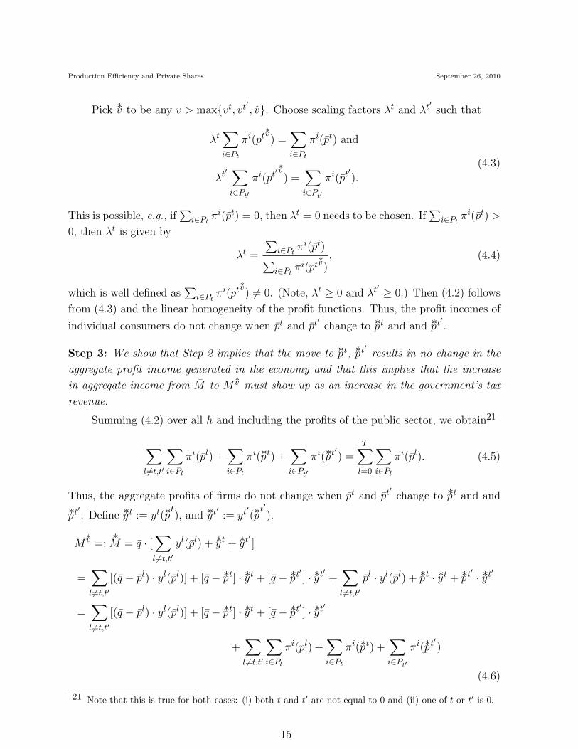
Pick ∗v to be any v > max{vt, vt′ , v}. Choose scaling factors λt and λt′ such that

λt∑

i∈Pt

πi(pt∗v) =

∑

i∈Pt

πi(pt) and

λt′∑

i∈Pt′

πi(pt′∗v) =

∑

i∈Pt′

πi(pt′).

(4.3)

This is possible, e.g., if∑

i∈Ptπi(pt) = 0, then λt = 0 needs to be chosen. If

∑

i∈Ptπi(pt) >

0, then λt is given by

λt =

∑

i∈Ptπi(pt)

∑

i∈Ptπi(pt

∗v), (4.4)

which is well defined as∑

i∈Ptπi(pt

∗v) 6= 0. (Note, λt ≥ 0 and λt′ ≥ 0.) Then (4.2) follows

from (4.3) and the linear homogeneity of the profit functions. Thus, the profit incomes of

individual consumers do not change when pt and pt′ change to ∗pt and and ∗pt′ .

Step 3: We show that Step 2 implies that the move to ∗pt, ∗pt′ results in no change in the

aggregate profit income generated in the economy and that this implies that the increase

in aggregate income from M to M∗v must show up as an increase in the government’s tax

revenue.

Summing (4.2) over all h and including the profits of the public sector, we obtain21

∑

l 6=t,t′

∑

i∈Pl

πi(pl) +∑

i∈Pt

πi(∗pt) +∑

i∈Pt′

πi(∗pt′) =T

∑

l=0

∑

i∈Pl

πi(pl). (4.5)

Thus, the aggregate profits of firms do not change when pt and pt′ change to ∗pt and and

∗pt′ . Define ∗yt := yt(∗pt), and ∗yt′ := yt′(∗p

t′

).

M∗v =:

∗M = q · [

∑

l 6=t,t′

yl(pl) + ∗yt + ∗yt′ ]

=∑

l 6=t,t′

[(q − pl) · yl(pl)] + [q − ∗pt] · ∗yt + [q − ∗pt′ ] · ∗yt′ +∑

l 6=t,t′

pl · yl(pl) + ∗pt · ∗yt + ∗pt′ · ∗yt′

=∑

l 6=t,t′

[(q − pl) · yl(pl)] + [q − ∗pt] · ∗yt + [q − ∗pt′ ] · ∗yt′

+∑

l 6=t,t′

∑

i∈Pl

πi(pl) +∑

i∈Pt

πi(∗pt) +∑

i∈Pt′

πi(∗pt′)

(4.6)

21 Note that this is true for both cases: (i) both t and t′ are not equal to 0 and (ii) one of t or t′ is 0.

15


Similarly,

M =T

∑

l=0

[(q − pl) · yl(pl)] +T

∑

l=0

∑

i∈Pl

πi(pl). (4.7)

Since∗M−M > 0, it follows from (4.5) that the government’s revenue from commodity

taxes is higher when we move to ∗pt, ∗pt′ keeping consumer prices and producer prices for

the firm groups other than t and t′ unchanged, that is,

∗G :=

∑

l 6=t,t′

[(q − pl) · yl(pl)] + [q − ∗pt] · ∗yt + [q − ∗pt′ ] · ∗yt′ >T

∑

l=1

[(q − pl) · yl(pl)] =: G.

(4.8)

Step 4: We show that the increase in the government’s revenue can be used to construct

another tax equilibrium where utility of at least one consumer is higher, with no loss in

utility for the others: this is obtained by either increasing the demogrant by an appropriate

amount (this is possible if (a) holds) or by decreasing (increasing) the consumer price of,

and hence the tax on, the kth commodity by an appropriate amount (this is possible if b(i)

(b(ii)) holds).

For all h define xh(q, rh +m+ q ·eh) =: xh,∑

h xh =: x, and e :=∑h eh. (4.2) implies

that for all h, xh = xh(q, ∗rh+m+q·eh). Since x ≤ y+e ≪∑

l 6=t,t′ yl(pl)+∗yt+∗yt′+e =: ∗y+e,

we have x ∈ {∗y + e} + RN−−.

Since xh is a continuous function of qk for all h, clearly, if condition b(i) or b(ii) hold,

we can apply the DM argument to find ∗q := 〈q−k,∗q k〉 and ∗ǫ such that (1)

∑

h xh(∗q , ∗rh +

m + ∗q · eh)) =:∑

h∗xh ∈ N∗ǫ (x) ⊂ {∗y + e} + RN

−− and (2) uh(∗xh) ≥ uh(xh) for all h and

uh(∗xh) > uh(xh) for some h.22 This implies that ∗s := 〈∗q , (pl)l 6=t,t′ ,∗pt, ∗pt′ , m〉 is another

tax equilibrium configuration of E(E,P , rP,p) that Pareto dominates s.23 This contradicts

the fact that s is a solution to (2.12).

If condition (a) holds, then we can exploit the continuity of xh in m for all h to find

m > m and ǫ such that (1)∑

h xh(q, ∗rh + m+ q · eh)) =:∑

h xh ∈ N∗ǫ (x) ⊂ {∗y − e}+RN−−

and (2) uh(xh) ≥ uh(xh) for all h and uh(∗xh) > uh(xh) for some h.24 This again leads to

a tax equilibrium that Pareto dominates s, which once again contradicts the hypothesis

of the theorem.25

22 Note, this implies reducing (increasing) the consumer price on commodity k that every one likes andhas a non-negative net demand (dislikes and has a non-positive net demand).23 Note that it is always possible to make the new tax equilibrium configuration conform to the normal-

ization rules adopted, e.g., if the normalization rules are p11 = 1 and p0

1 = 1 and if t 6= 1, 0 and t′ 6= 1, 0,

then divide 〈∗q , (pl)l 6=t,t′,0,∗pt, ∗pt′ , m〉 by p1

1 and p0 by p01.

24 Note, this is made possible by the fact that∗G > G in (4.8), so that it is possible to distribute all or

a part of this increased government budget-surplus as a higher demogrant.25 Once again, the new tax equilibrium can be reconfigured to conform to our normalization rules.

16


5. Corollaries of Theorem 1:

Two results follow as corollaries of Theorem 1.

Corollary 1 of Theorem 1: Production efficiency is desirable at the second-best of a

profit-making economy with firm-group specific profit taxes.

Proof:

Step 1: We show that the set of tax equilibrium allocations of E(E,P , rP,τ ) is a subset of

the set of tax equilibrium allocations of E(E,P , rP,p).

Let ατ := 〈q, p, p0, τ1, . . . , τT , m〉 be a tax equilibrium of a profit-making econ-

omy with firm-group specific profit taxes E(E,P , rP,τ ) associated with a partition P =

{P1, . . . , PT} of I\{0} and a map of profit incomes rP,τ . Define αp := 〈q, p0, p1, . . . , pT , m〉

with pt := (1 − τ t)p for all t = 1, . . . , T . Let E(E,P , rP,p) be a profit-making economy

with firm-group specific prices, where26

rP,p(a) = rP,τ (a). (5.1)

For all t = 1, . . . , T , the linear homogeneity of the profit function implies∑

i∈Ptπi(pt) =

(1 − τ t)∑

i∈Ptπi(p), and for all h ∈ H, we have

rhP,p(

∑

i∈P1

πi(p1), . . . ,∑

i∈PT

πi(pT ) ) = rhP,τ ( (1 − τ1)

∑

i∈P1

πi(p), . . . , (1 − τT )∑

i∈PT

πi(p) ).

(5.2)

This implies that αp is a tax equilibrium of E(E,P , rP,p) that results in the same allocation

as ατ in economy E(E,P , rP,τ ).

Step 2: We show that every second-best of E(E,P , rP,p) can be decentralized as a tax

equilibrium of E(E,P , rP,τ ).

Theorem 1 implies that if 〈q, p0, p1, . . . , pT , m〉 is a second-best of E(E,P , rP,p), then

there exist positive scalars λ2, . . . , λT such that pt = λtp1 for all t = 2, . . . , T . Choose

p = p1, τ1 = 0, and τ t = 1 − λt for all t = 2, . . . , T . Then 〈q, p, p0, τ1, . . . , τT , m〉 is a tax

equilibrium of E(E,P , rP,τ ).

Steps 1 and 2 imply that production efficiency is desirable at the second-best of

E(E,P , rP,τ ).27

Corollary 2 of Theorem 1: If profit taxes cannot be implemented then intermediate-

inputs should be taxed proportionately. Alternatively, firm-specific profit taxation justifies

not taxing inter-firm transactions in profit making economies.

26 Recall the definitions of maps of profit incomes for firm-group specific profit taxes and firm-groupspecific prices in Sections 2.27 Of course, this follows under the conditions laid down in Theorem 1 as translated to economyE(E,P, rP,τ ).

17


Proof: Consider a profit-making economy with firm-group specific prices E(E,P , rP,p).

Let P be a partition of I \ {0}. Thus, the government can implement firm-group specific

prices in such an economy. This means that non-zero wedges are allowed between price

vectors faced by any two groups of private firms in this economy, e.g., pt−pt′ is the wedge

between the price vectors pt ∈ RN+ and pt′ ∈ RN

+ faced by private firms in firm-groups t and

t′, respectively. Thus, transactions that happen between these two groups of private firms

are effectively taxed. Thus, this economy permits a very general system of intermediate

input taxation. Theorem 1 demonstrates, however, that at the second-best of such an

economy producer prices are proportional to each other, e.g., if 〈q, p0, p1, . . . , pT , m〉 is a

second-best of E(E,P , rP,p), then there exist positive scalars λ2, . . . , λT such that pt = λtp1

for all t = 2, . . . , T , where p1 is the price vector for firms in group 1. Thus, the wedge

between price vectors of firm-groups t and t′ at this second-best is p1(λt−λt′). Transactions

in commodities between these two firm-groups are, hence, taxed proportionately at a rate

λt − λt′ . Alternatively, from Corollary 1 of Theorem 1 (above) it follows that this second-

best can be decentralized as a second-best tax equilibrium of a profit-making economy

with firm-group specific profit taxes. But this precludes intermediate goods taxation as

all firm-groups face the same producer price p1 in this economy. Rather, firm-groups are

subject to firm-group specific profit tax rates τ t = 1 − λt for all t = 1, . . . , T . It is in this

sense that Corollary 2 of Theorem 1 follows.

As a special case, the famous implication with regards to intermediate input taxation

for DM and Guesnerie [1995] models follows:28 If government can implement one-hundred

percent profit taxation and redistribute proceeds to consumers as a demogrant, then in-

termediate input taxation is not desirable.

6. Conclusions.

There is a classic literature that studies the desirability of production efficiency in

economies with Ramsey taxation where firms make positive profits which can potentially

be partly taxed away and partly distributed back to consumers. The results of this classic

literature are often invoked to justify the use of producer prices as proxies for shadow

prices in cost-benefit tests of marginal public sector projects. We show that the desirabil-

ity of second-best production efficiency depends on the link between the constraints on

government’s profit taxation power and the institutional rules by which (profit) incomes

are distributed in the economy. We generalize results in the literature by showing that

second-best production efficiency is desirable whenever firms can be organized into groups

such that (i) profit tax rates vary across these groups and (ii) consumer incomes depend on

28 Recall, this case is equivalent to the case where P is the coarsest partition of private firms, i.e.,

P = {I \ {0}} and θhi = 1

Hfor all h and i ∈ I \ {0}.

18


the distribution of profits across these groups. Thus, the fewer (larger) the number of firm-

groups, the lesser (more) are the profit tax rates that are required to ensure second-best

production efficiency. The two cases studied in the literature of firm-specific and uniform

(e.g., one-hundred percent) profit taxation follow as two special cases of our general result.

The result follows because, at any production inefficient status-quo of such economies,

the private sector producer price vector and the prices in the public sector (the latter re-

flect the true shadow prices in the economy) are not proportional. The differences in the

marginal rates of substitution in the private and public sectors imply that production

can be reallocated between these sectors to increase aggregate output and income in the

economy. Lemma 1 proves that, in an institutional structure where producers are price

takers and maximize profits, small changes in the two price vectors can be constructed

that ensure that this potential increase in the aggregate output can be supported as profit

maximizing choices of firms. The continuity and linear homogeneity of the profit func-

tion imply that by implementing firm-group specific profit taxation, the government can

effectively implement further (but proportionate) changes in producer prices that ensure

that the net of tax firm-group profits, and hence the profit incomes of the consumers that

depend on the distribution of the firm-group profits, remain at the status-quo levels, while

at the same time there are no further changes in the (increased) supply by firms. This

must mean that the increase in aggregate income shows up as an increase in the tax and

public sector incomes of the government, which can be used to change commodity taxes

or to increase demogrant incomes of people in a Pareto improving way. Thus, there are

always Pareto improvements at any production inefficient status-quo of such economies.

The mechanism suggests why this strategy does not work, generally, in most private

ownership economies when restrictions on profit taxation are not consistent with the rules

of income distribution as outlined above in (i) and (ii). This is because, while a production

inefficient status-quo suggests that there are changes in producer prices that can increase

the aggregate output in the economy, any attempt by the government to change profit

tax rates to maintain net of tax profits at the status-quo levels, may not translate into

maintaining profit incomes of the consumers at the status-quo levels. Thus, all of the

increased output may not, in general, become available to the government for designing

Pareto improving changes in taxes and demogrant. Private ownership diverts some of the

increased resources from the government coffers and puts it into the hands of consumers

as profit incomes. But the private ownership structure could be such that it may lead to

an inequitable distribution of profit incomes and a decrease in welfare of some consumers,

which no government policy may be able to correct with the remaining resources, that

is, there may exist no directions of change in the government policy instruments that

are Pareto-improving, equilibrium preserving, and compatible with the existing private

ownership structure. Our analysis hence suggests how, by understanding the rules of

19


profit income distribution in the economy, the government can potentially design profit

taxation that can promote both its redistributive and efficiency objectives.

We also show that in economies with Ramsey taxation where consumers also receive

profit incomes, proportionate intermediate input taxation is recommended in the absence

of profit taxation. Alternatively, profit taxation is a perfect substitute for intermediate

input taxation. The classic result of DM (extended as in Guesnerie [1995] to take account

of profit making economies) on no intermediate input taxation follows as a special case of

our model with profit taxation where all firms are subject to one-hundred percent profit

taxation with the tax proceeds being redistributed back to consumers as a demogrant.

In this sense, the recommended structure of intermediate input taxation also serves both

efficiency and redistributive objectives of the government and supports tax systems such

as VAT.

APPENDIX

Proof of Lemma 1. Smoothness of Y t and Y t′ implies that H(pt, pt · yt(pt)) and

H(pt′ , pt′ · yt′(pt′)) are unique supporting hyperplanes for Y t and Y t′ at yt(pt) and yt′(pt′),

respectively.

Step 1. Since pt and pt′ are not collinear, H(pt, 0) is not a supporting hyperplane for

H≥(pt′ , 0) and H(pt′ , 0) is not a supporting hyperplane for H≥(pt, 0) at 0N . This implies

that there exist ∆yt ∈ RN and ∆yt′ ∈ RN such that the following is true:29

∆yt ∈ H<(pt, 0) ∩ H≥(pt′ , 0),

∆yt′ ∈ H<(pt′ , 0) ∩ H≥(pt, 0), and

∆yt + ∆yt′ ≫ 0N .

(A.1)

This implies that yt(pt) + yt′(pt′) + ∆yt + ∆yt′ ≫ y. Denote yt(p) by yt and yt′(pt′) by

yt′ . Since yt and yt′ belong to Y t and Y t′ , Assumption 3 implies that f t(yt) = 0 and

f t′(yt′) = 0.

Step 2. Recall that ∇f t(yt) is defined as the linear mapping such that for all {hv} → 0N ,

we have

limhv→0N

f t(yt + hv) − [f t(yt) + ∇f t(yt)hv]

|hv|≡ lim

hv→0N

e(hv, yt)

|hv|= 0, (A.2)

where e(hv, yt) = f t(yt +hv)− [f t(yt)+∇f t(yt)hv]. We show that there exists γt > 0 such

that ∇f t(yt) = γtpt. Take any point y ∈ Y t such that y 6= yt. Then, from the convexity

29 The intuition becomes clear when one sees Figure 1.

20


of Y t, f t(yt + λ(y − yt)) ≤ 0 for all λ ∈ [0, 1]. Using (A.2) and the fact that f t(yt) = 0,

we have

∇f t(yt)(y − yt)

| y − yt |= lim

λ→0

f t(yt + λ(y − yt)) − f t(yt)

| y − yt |λ= lim

λ→0

f t(yt + λ(y − yt))

| y − yt |λ≤ 0. (A.3)

Since this is true for all y ∈ Y t, ∇f t(yt) is a normal to a supporting hyperplane of Y t at

yt. Since, Y t is smooth and H(pt, pt · yt) is also a supporting hyperplane of Y t at yt, there

must exist γt > 0 such that ∇f t(yt) = γtpt. Similarly, we can prove that there exists

γt′ > 0 such that ∇f t′(yt′) = γt′ pt′ .

Step 3. (A.3) implies that ∆yt · ∇f t(pt) < 0 and ∆yt′ · ∇f t′(pt′) < 0. Choose a sequence

{λv} such that λv∆yt → 0 and λv > 0 for all v. We now show that there exists v′ such

that for all v > v′, we have ytv := yt + λv∆yt ∈ Y t. From (A.2) we have

limλv→0

f t(yt + λv∆yt) − f t(yt) − λv∇f t(yt)∆yt

|∆yt |λv= 0. (A.4)

Since f t(yt) = 0 and ∇f t(yt)∆yt < 0 (from Step 2), we have

limλv→0

f t(yt + λv∆yt)

|∆yt |λv=

∇f t(yt)∆yt

|∆yt |< 0. (A.5)

Hence, there exists a large enough v′ such that for all v > v′, we have f t(yt + λv∆yt) < 0,

and hence ytv := yt + λv∆yt ∈ intY t for all v > v′.30 Similarly, we can prove that there

exists v′′ such that for all v > v′′, we have yt′v

:= yt′ + λv∆yt′ ∈ intY t′ .

Step 4. We now show that there exist sequences {ptv} and {pt′v}, and a positive integer

v such that for all v > v, we have yt(ptv) + yt′(pt′v) ≫ yt + yt′ . Define v = max{v′, v′′}.

For every v > v, ytv ∈ Y t. It can therefore be shown that there are continuous maps

κt(ytv) := maxκ {κ ≥ 0∣

∣[ytv + κ1N ] ∈ Y t} and κt′(yt′v) := maxκ {κ ≥ 0

∣

∣[yt′v

+ κ1N ] ∈

Y t′}.31 For all v > v, it is clear that (i) ytv + yt′v≫ yt + yt′ and so (ytv + κt(ytv)1N ) +

(yt′v

+ κt′(yt′v)1N ) ≫ yt + yt′ , (ii) (ytv + κt(ytv)1N ) and (yt′

v+ κt′(yt′

v)1N ) belong to

Y t and Y t′ , respectively, and (iii) {ytv + κt(ytv)1N} → yt and {yt′v

+ κt′(yt′v)1N} →

yt′ . Define ptv = 1

γt∇f t(ytv + κt(ytv)1N ) and pt′v

= 1

γt′∇f t′(yt′

v+ κt′(yt′

v)1N ). The

smoothness of functions f t and f t′ imply that {ptv} → pt and {pt′v} → pt′ . Clearly,

yt(ptv) = ytv + κt(ytv)1N and yt′(pt′v) = yt′

v+ κt′(yt′

v)1N , so that for all v > v, we have

yt(ptv) + yt′(pt′v) ≫ yt + yt′ .

30 For any set A ⊂ Rn, intA is the interior of A relative to R

n.31 Assumptions 1 and 2 guarantee the existence of such maps.

21


Hence, for all v > v, the conclusions of the lemma follow for sequences {ptv} and

{pt′v}.

REFERENCES

Cornet, B., Existence of Equilibria in Economies with Increasing Returns in Contributionsto Operations Research and Economics: The Twentieth Anniversary of CORE,editors: B. Cornet and H. Tulkens, Cambridge, Massachusetts: MIT Press, 1989.

Boadway, R., “Cost Benefit Rules in General Equilibrium” Review of Economic Studies39, 1972, 87-103.

Dasgupta, P. and J. Stiglitz, “On Optimal Taxation and Public Production” The Reviewof Economic Studies 39, 1972, 87-103.

Diamond, P. and J. Mirrlees, “Optimal Taxation and Public Production I: ProductionEfficiency” The American Economic Review 61, 1971, 8-27.

Diamond, P. and J. Mirrlees, “Optimal Taxation and Public Production II: Tax Rules”The American Economic Review 61, 1971, 261-278.

Dreze, J. and N. Stern, The Theory of Cost Benefit Analysis in Handbook of PublicEconomics, editors: A. J. Auerbach and M. Feldstein, II, Chapter 14, Elsevier SciencePublishers, North Holland, 1987.

Hahn, F., “on Optimum Taxation” Journal of Economic Theory 6, 1973, 96-106.Guesnerie, R., A Contribution to the Pure Theory of Taxation, Cambridge, UK: Cambridge

University Press, 1995.Little, I. M. D. and J. Mirrlees, Project Appraisal and Planning for Developing Countries,

Heinemann Educational Books, London, 1974.Mirrlees, J., “On Producer Taxation” Review of Economic Studies 39, 1972, 105-111.Munk, K. J., “Optimal Taxation with Some Non-Taxable Commodities” Review of

Economic Studies 47, 1980, 755-765.Myles, G. D., Public Economics, Cambridge, UK: Cambridge University Press, 1995.Ramsey, F., “A Contribution to the Theory of Taxation” The Economic Journal 37, 1927,

47-61.Reinhorn, L., “Production Efficiency and Excess Supply” A Draft, 2010.Rockafellar, R.T., “Clarke’s Tangent Cones and the Boundaries of Closed Sets in Rn,”

Nonlinear Analysis, Theory and Applications 3, 1978,145–154.Sadka E., “A Note on Producer Taxation” Review of Economic Studies 44, 1977, 385-387.Weymark J., “On Pareto Improving Price Changes” Journal of Economic Theory 19, 1978,

338-346.Weymark J., “A Reconciliation of Recent Results in Optimal Taxation Theory” Journal

of Public Economics 12, 1979, 171-189.

22

Documents

Economics Department Discussion Papers Series