Discussion Papers in Economics - york.ac.uk · Discussion Papers in Economics Department of Economics and Related Studies University of York ... Economic geography models see each

Discussion Papers in Economics

Department of Economics and Related StudiesUniversity of York

HeslingtonYork, YO10 5DD

No. 12/16

Should I Stay or Should I Go? Intra-provinceMigration in Guangdong

Peter Simmons & Yuan Yuan Xie

Should I Stay or Should I Go? Intra-provinceMigration in Guangdong

Peter Simmons & Yuan Yuan XieDepartment of Economics, University of York

June 6, 2012

Abstract

Guangdong is one of the fastest growing Chinese provinces and has ahigh level of gross migration �ows. Its intra-province migration is 2.7 timeshigher than its inter-province migration. We study migration between the18 prefecture-level divisions of Guangdong during 1990-1999 using annualdata. In our framework, migration decisions are based on di¤erences in�ve characteristics between origin and destination: expected urban wage,marriage opportunities, urbanisation and (to re�ect pro�tability ofself employed migrants) population and capital stock. We formu-late a panel regression equation allowing for both panel heteroscedasticityand inter-cities heterogeneity in the migration process. Remarkably we�nd that there is a high degree of homogeneity between cities, the onlydi¤erences being in the impacts of capital stock and degree of urbanisa-tion. Even here, nearly 70% of cities have identical e¤ects. Despite thehigh level of net migration demonstrated to be largely causedby the above characteristics, intercity inequalities as measuredby some of these forces has been growing over our time period.This suggests that a locational equilibrium has not yet been achieved.

Key words: Intra-provincial migration; intercity inequalities; multi-variate choices; equilibrium.

JEL: J61 O15 R23

1

1 Introduction

The remarkable economic transformation of China over the last 30 years has

partly resulted from regional economic development, with construction of in-

frastructure and establishment and growth of an industrial base concentrated

in particular areas. This has stimulated internal migration on a large scale

both from rural to urban areas, and between urban areas which are growing at

di¤erent rates. Some migration is relatively long distance e.g. cross province

migration, generally from the west to the east, but the same phenomenon also

exists on a smaller scale within provinces.

Guangdong is one Chinese province which was singled out for regional devel-

opment in 1985 and since then has had a high volume of cross province immi-

gration. The Guangdong cities Shenzhen, Zhuhai and Shantou around the Pearl

River Delta regions have been special economic zones1 with favourable govern-

ment industrial development incentives since 1980. The special economic zones

were chosen as a result of convenient communication and transportation capa-

bilities from and to overseas countries, especially Macao and Hongkong (Ateno,

1979). In addition, rapid industrialisation has been facilitated by high FDI (for-

eign direct investment) especially that arising from the geographical and social

proximity to Hong Kong Subsequently, industrial and trade areas have �our-

ished especially around the Pearl River, triggering high levels of intra-province

migration. According to the provincial census, in 1990, Guangdong is one of

the provinces with the highest inter-province migration and its intra-province

migration is 2.7 times greater than its inter-province migration. Earlier work

1The special economic zone "can be de�ned as an area where enterprises are treated morepreferentially than in other areas in relation to such matters as the tax rate and the scopeof operations in order to attract foreign capital and advanced technology for modernisation"(Ateno, 1979)

2

on immigration in Guangdong used census data from 1990 and found economic

employment factors to be the dominant cited factor for inter-province migration,

followed by social reasons including marriage. Guangdong itself is divided into

18 city areas, each one including both an urban part and a rural part, of varying

relative importance. Thus, city-city migration within Guangdong encompasses

all mixes of urban/rural origins and destinations.

Economic models of migration can be put in a general framework in which

each possible location is perceived by an individual to have costs and bene-

�ts. Migration occurs when the net gain from changing location exceeds the

migration cost. Economic geography models see each location as having some

attracting and repelling forces. Taken together, these can develop positive and

negative synergies which result in a particular spatial and size pattern of settle-

ments as individuals move in response to these net bene�ts. (Krugman, 1992).

A stark version of this is a Harris-Todaro model (Harris & Todaro, 1970), in

which the standard of living or net bene�t of a region is measured just by the

expected labour income it o¤ers. In these modelling approaches, an equilibrium

spatial population distribution arises when no individual sees a net bene�t from

leaving its current location. However, there are some caveats. One is the time

horizon and permanence attached to the migration decision. A move may be

planned to be temporary, or even partial if just some members of the family

migrate and the stayers maintain an economic base in the origin location. If cir-

cumstances change after migration has occurred, it may induce a new round of

migration or even a return migration. Through commuting/guest working, lo-

cational bene�ts may be realised without changing residence. In addition, there

are costs and barriers to migration. The hukou system plays an important role

3

in determining the opportunity set in the destination area because it introduces

a local residence passport, whose possession gives access to public services like

education and also a di¤erential access to the labour market.

The aim of this paper is to develop a theoretical framework appropriate for

empirical analysis of migration patterns. To achieve our aim, we build a regres-

sion model with dependent variable the net migration between each of the 18

prefecture-level divisions of Guangdong2 . Using data from the Guangdong City

Yearbook for 1990-1999, we test this framework on panel data using GLS and

weighted least squares. Nonzero covariances between the shocks to net migra-

tion for one city and another and heteroscedasticity within each year over time

are allowed. We test for validity of the speci�cation at each stage in terms of

covariance and autocorrelation assumptions and for validity of the mean spec-

i�cation. The determinants of net migration are intra-city di¤erentials in the

following �ve characteristics: expected urban wage, population, capital stock,

marriage opportunities and urbanisation. We test for equality of coe¢ cients on

the net migration determinants between cities. Remarkably we �nd that there is

a high degree of homogeneity between cities. Only a few cities and determinants

(especially capital stock and the degree of urbanisation) display some hetero-

geneity in the migration process. Our results are valid speci�cations according

to heteroscedasticity, panel serial correlation and reset/link speci�cation tests.

In a locational equilibrium, the net bene�ts of moving between cities should

be equalised. In fact inequality between cities in some of the relevant factors has

increased not fallen over our sample. The coe¢ cient variation of urban/rural

income and capital stock per capita suggest that inequalities between cities

2Due to changes in city boundaries, we construct these from the underying 21 cities toderive city areas that exist for each sample date (see 2.2 below).

4

are increasing over time. The capital city (Guangzhou) and the two special

economic zones (SEZ: Shenzhen and Zhuhai) are urban wage leaders. The two

SEZ�s concentrate on high technology industry and share high capital stock per

person at a level even exceeding that of the "four tigers" of the manufacturing

sector: Dongguan, Zhongshan and Foshan3 . Some other city attributes show

either stable (single female and city population) or falling (the urbanization

level and late marriage rate) cross-city inequality over time. Taken together,

the rising inequality in some migration inducing factors may imply that a full

locational equilibrium has not yet been achieved.

Section 2 gives a brief literature review, section 3 develops the theoretical

framework, section 4 describes the data, outlines the econometric strategy and

presents the empirical results. Second 5 contains a conclusion.

2 Previous Studies

Fan (1996, 1999, 2003) has carried out qualitative study of Guangdong migration

based on the 1990 census. Her focus is relatively aggregate compared with ours

so that population movement is broken down into inter-province and intra-

province but does not have a �ner classi�cation than this. She �nds high levels

of both inter- and intra-province movement but relatively higher levels of the

latter. Most of her focus is on inter-province migration. Interestingly, marriage

migration is concentrated more in inter- than intra-province moves. About 7%

and 5% of male and female migrants moved for job transfer reasons mainly

in professional, government or administrative occupations but the predominant

reason for migration (around 60%) of moves were for industry/business reasons

de�ned o¢ cially as moving to seek or take up employment as a labourer in

3Two tigers are located in Foshan.

5

industry or business. This predominance of employment seeking reasons held

for both genders although for women, marriage migration was more important

than for men (around 8%):The majority of her migrants held an agricultural

hukou in their origin location (65%) and not all of these transferred to an urban

hukou in their destination location. In summary, although a formal model is

not used, her evidence is consistent with explaining migration in terms of the

net advantages of di¤erent locations.

Zhu (2002) uses data from a survey of 2573 households in Hubei province in

1993 to study intra-province migration. Respondents are either in the metropo-

lis (Wuhan) or in a medium sized city (Danjiangkou) or in non-urban areas.

For a subsample who retain their original hukou (thought of as either rural non-

migrants or rural-urban migrants if the address changed in the period 1988-

1993), the paper estimates a probit for each gender with dependent variable

the migrant/nonmigrant status and with urban and rural income treated as en-

dogenous with possible sample selection bias. A two step Heckman approach

is used. In the income equations, personal characteristics (age,education) and

also the GDP per capita of the current location matter. There is no evidence

of sample selection bias. In the structural probit equation, predicted income is

highly signi�cant. In his sample, there is some evidence of a signi�cant di¤er-

ence in marital status pre and post migration and hence of migration for reasons

of marriage. Zhu et al. (2009) use survey data from 2006 of temporary residents

located in nine major industrialised cities around the Pearl River delta (the pop-

ulation of these cities in 1990 was 57% composed of agricultural hukou holders).

Just over half the 3000 respondents were single and generally of relatively low

education and young (mean age 27). Intra-Guangdong migration accounted for

6

22% of the sample, with Shenzhen being the predominant destination. The pa-

per estimates the time to �nding urban employment for temporary residents (a

hazard function) and an accelerated lifetime model. Interestingly women �nd

urban employment more rapidly on average than men. In part this is due to

di¤erences in the jobs taken up by women, which are typically lower paid less

skilled jobs than for men.

The existing theories of economic interaction between regions/cities have

been applied to western economies and are mainly covered by urban and geo-

graphical economics. Harris developed the idea of "market potential" and he

pointed out that each region has a di¤erent desirability which depends on its

market potential (Harris, 1954). The market potential is an index which is the

sum of incomes of all regions weighted by the distance between this region and

others. A highly developed region grows where there is a large market, and this

market is then augmented by the growth of the industry of this region. So there

is a circular relationship between market potential and growth of regional in-

dustries. Myrdal (1957) suggests "cumulative causation" which means that the

initial stimulus of a large market attracts new industries and the growth of these

industries subsequently enlarges the local markets. Krugman (1992) claims that

there are "centripetal" forces and "centrifugal" forces which pull economic ac-

tivity into or away from agglomerations. Regions with di¤erent levels of "market

potential" have di¤erent capabilities of pulling individuals to come and pushing

local residents to leave. The "cumulative causation" suggests that the well de-

veloped regions could attract migrants to work for their industries, and growth

of these industries could enlarge the local labor markets leading to subsequent

additional immigration. The balance of "centripetal" and "centrifugal" forces

7

of each region results in net migration �ows between locations..

The Harris-Todaro framework balances the bene�ts of migration with its

costs. Few prior studies on regional migration in China have used formal the-

oretical models of migration cost. Poncet (2006) is one exception who tries to

capture the spatial cost of migration in a sample for the whole of China through

a mixture of physical distance between origin and destination and the number of

province boundaries which must be crossed in the migration process. However

this approach is less applicable to intra-province migration within Guangdong

since surface transport journey times between the extremities of Guangdong are

a matter of just a few hours.

In summary earlier work on Guangdong migration suggests that it is econom-

ically motivated but has been limited in its use of formal structural economic

models to guide the empirical analysis. It also has only been able to distinguish

micro-geographical city e¤ects to a limited extent. In this paper we use city

based data to do this, together with a simple formalisation of a Harris Todaro

style framework to condition the empirical analysis in a multi-location context.

3 Theoretical background

Anyone living in city j has multiple choices to move to one of the remaining 17

cities i (i=1...17 and i6= j) so this movement allows rural-urban, urban-urban

and rural-rural moves between cities. There may be multiple reasons for mov-

ing. As the data suggests, there are three key employment three chief employing

organisations within a city but then a much larger ancillary range of jobs. The

measured unemployment in each city is very low, but nevertheless Zhu�s work

and other evidence suggests that migrants who move without a prearranged job,

8

especially those who retain agricultural hukou status, take time to �nd one and

then it is often in the informal rather than the formal sector. Household level

data on Chinese migration also suggests that moving to become self-employed

through establishment of a family business is also important (RUMiCI ,2007).

In addition, migrants also move for non-labour market reasons such as marriage

and joining relatives and friends, to take advantage of the better infrastructure

of an urban region. So we need a framework including each of these elements. A

pure HarrisTodaro approach sees migration as determined by the di¤erence be-

tween the expected wage in the destination city (measured by the unemployment

rate multiplied by the wage) and wage in the origin city, net of the migration

cost. This is not immediately applicable since the reported unemployment rate

is close to zero and it only covers some of the migration reasons. The Krug-

man approach more generally would include the expected wage income gap as

a factor but add other possible factors to this such as the synergies o¤ered by a

concentration of industrial �rms leading to a �uid labour market, the additional

motives such as marriage.

Adapting this approach we allow for four reasons to move from i to j :

(a) to work as an employee in the three chief employing organisations4 in j; in

which case the primary motivation is an expected real wage di¤erence between

cities

(b) to be selfemployed in j; where the di¤erence in pro�t opportunities be-

tween i and j accounts for the move.

(c) get married/join friends etc who are in j: One measure of the relative

desirability of di¤erent cities in their marriage opportunities is given by the

4These are either state or urban collective units, or private sector units with joint ownership,shareholding or foreign ownership (ie excluding self employment).

9

gender structure of the population of single individuals in di¤erent cities.

(d) to leave a mainly agricultural city area to move to a more urbanised city

area where infrastructure is better developed

Individuals in i are heterogeneous and the emigrants are those who at present

in i have the worst opportunities. If we think of the distributions of wages, self

employment pro�ts, marriage and urban opportunities in i then it will be the

individuals in the lower parts of these distributions who will have the highest

desire to emigrate to a city with better prospects. Any such individual does

not know the exact outcome if he does move, but has a chance of securing the

mean prospects of city j to which they move. If the average expected wage

in the top three sectors in j is wj , the average return to self-employment or

other work in j (like pro�ts) is �j(Pj ; kj) which depends on population Pj and,

capital Kj , the individuals in the lower part of the wage or pro�t distribution of

i compare their current situation with wj ; �j and use this to calculate the gain

from moving: Similarly for marriage, m, and urban opportunities, u, individuals

in i compare their current situation with the average situation of other city

prefecture-level divisions. Guangdong province has 18 prefecture-level cities.

If moving costs were similar between any pair of cities, individuals looking to

move for a particular reason will select to move to the city with the highest net

bene�t. For example an employed individual wishing to move to improve their

expected wage will plan to move to the city area with the highest expected

wage if that is higher than their current wage. Thus all employees currently

outside the top mean expected income city, and whose actual wage is below the

expected wage of the top city, will wish to move to the top expected income

city. Those employees currently in the city with the top mean expected wage

10

but whose individual wage is relatively low, and below the mean expected wage

of the second ranked city, will wish to move to the city with the second highest

mean expected wage. So for any of the reasons for moving, planned moves will

be moving from lower expected return cities to the highest expected return city,

except for individuals currently living in the highest expected return city but

whose individual payo¤ from living there is lower than the mean expected payo¤

from the second city.

De�ne the (cumulative) distributions5 of wages, self-employed pro�ts, mar-

riage chances and urban prospects within city i respectively by Fwi; F�i; Fmi; Fui

so eg Fwi(wj) = Pr(wih � wj) for individuals h in i: Let 1(x) be the top mean

return city for moving reason x and 2(x) be the city with second best return for

moving reason x = w; �;m; u: The % of individuals in the relevant subpopula-

tion who may wish to move is given by the distribution function of the factor x

in their current city evaluated at the mean return of the best alternative city.

For example a % Fwi(w1(w)) of urban hukou holding employees currently living

in i will have the desire to move to the top ranked expected wage city and the

number of such workers who wish to move from i to 1(x) to improve their wage

is given by Fwi(w1(w))Ui where Ui is the number of urban hukou holders in i:

Of those employees now living in 1(w); a number F1(w)(w2(w))U1(w) will wish

to move to city 2(w): Only cities 1(w); 2(w) will be the destination for desired

migration and the only employees wishing to move into 2(w) will be the em-

ployees of city 1(w) whose individual wage is below the mean expected wage of

city 2(w): The same approach applies to the factors �;m; u:

Any particular city i can be top or second ranked on one or more factors.

On any factor for which it is top, there will be desired immigration from all

5We assume that these distributions are independent.

11

other cities. For any factor on which it is second top there will be desired

immigration from low return individuals currently in the top ranked city for

that factor. If Sj ;Mj ; Hj are respectively the numbers of people in any city i

who are self employed, a¤ected by marriage opportunities, a¤ected by the urban

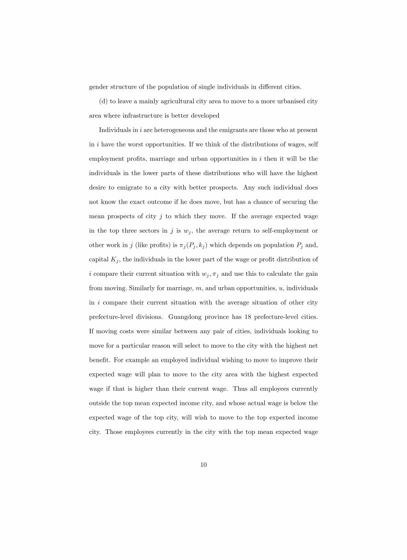
infrastructure, then total desired net migration (net immigration) into city i can

be written as6

NMi = �xf[�j 6=iFxj (xi)Xj � Fxi(x2(x))Xi if i = 1(x)]

+[F1(x)(x2(x))X1(x) � F2(x)(x1(x))X2(x) if i = 2(x)]g

�[Fxi(x1(x))Xi if i 6= 1(x); 2(x)]g

Individual h in city i can wish to move for any of the four reasons and will

have a desire to move according to the gap between the current position in i

and the prospects in other cities j:

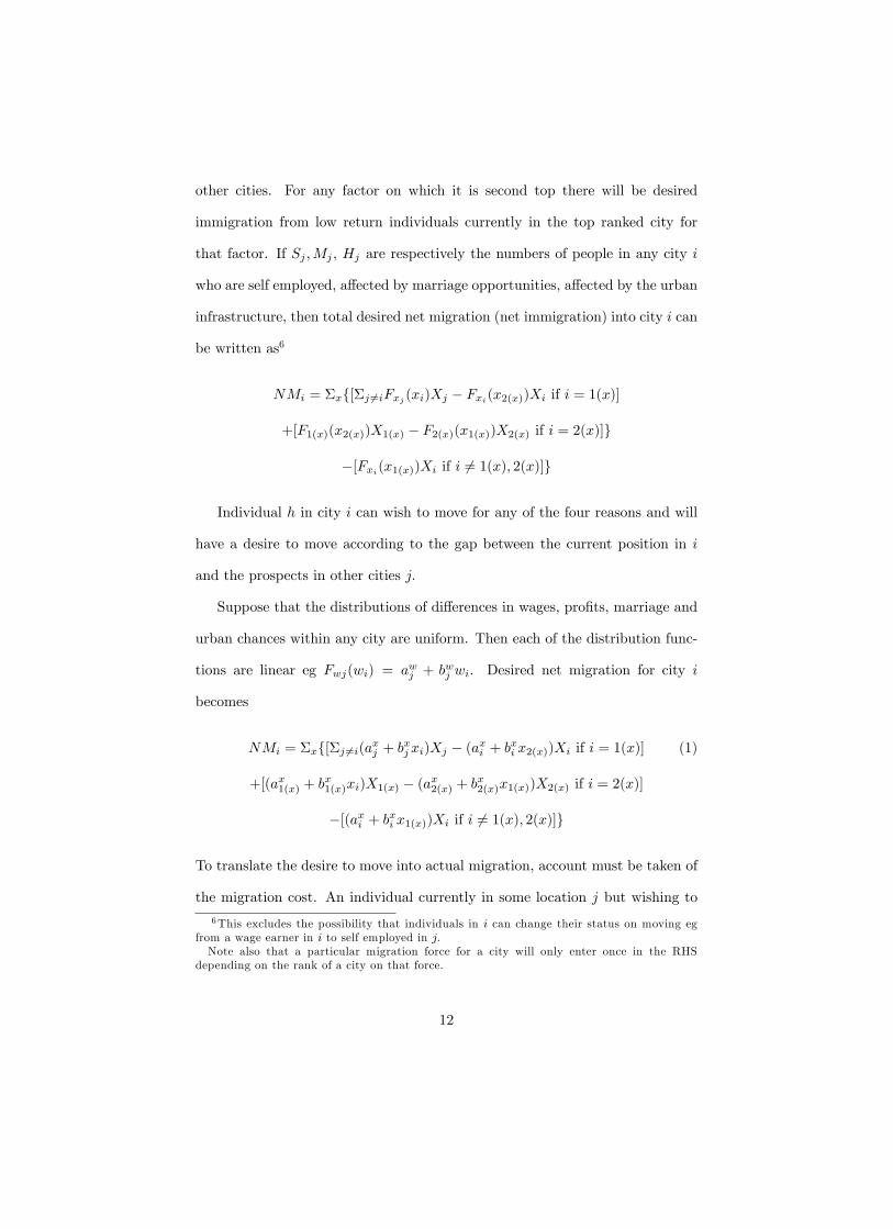
Suppose that the distributions of di¤erences in wages, pro�ts, marriage and

urban chances within any city are uniform. Then each of the distribution func-

tions are linear eg Fwj(wi) = awj + bwj wi. Desired net migration for city i

becomes

NMi = �xf[�j 6=i(axj + bxj xi)Xj � (axi + bxi x2(x))Xi if i = 1(x)] (1)

+[(ax1(x) + bx1(x)xi)X1(x) � (ax2(x) + bx2(x)x1(x))X2(x) if i = 2(x)]

�[(axi + bxi x1(x))Xi if i 6= 1(x); 2(x)]g

To translate the desire to move into actual migration, account must be taken of

the migration cost. An individual currently in some location j but wishing to

6This excludes the possibility that individuals in i can change their status on moving egfrom a wage earner in i to self employed in j:Note also that a particular migration force for a city will only enter once in the RHS

depending on the rank of a city on that force.

12

move to i will face an individually speci�c moving cost which will have common

factors across individuals due to common entry costs into i: The moving cost

into i thus results in a distribution Fi(z) of the number of latent immigrants

into i whose moving cost is low enough to result in a move. Thus observed net

migration into i, NMOi; can be written as NMOi = Fi(z)NMi:

NMOi = Fi(z)�xf[�j 6=ibxj xiXj � bxi x2(x))Xi if i = 1(x)] (2)

+Fi(z)[bx1(x)xiX1(x) -b

x2(x)x1(x)Xi(x) if i = 2(x)]

�Fi(z)[bxi x1(x)Xi if i 6= 1(x); 2(x)]g

The variables in z should be determinants of the city speci�c distributions of

moving costs for migrants planning to enter i: An obvious candidate is a measure

of the hukou cost or land/housing cost in i: This generates an empirical model

for understanding net migration rates between cities which encompasses the

motivations for migration found in prior research.

4 Empirical evidence

4.1 Guangdong City Areas and IntraGuangdong Migra-tion

The data comes from the Guangdong Statistical Yearbooks for the period 1990-

1999. Guangdong is divided into a maximum of 21 city areas but one of these,

Jieyang (city 20) was only established in 1992 taking over some parts of Shan-

tou (city 4). Moreover some parts of Chaozhou (city19) were formerly part of

Shantou (city4) before 1992. We merge these 3 city areas into a single unit (city

22). In addition Yunfu (city21) formerly was part of Zhaoqing (city17) before

1994, so we merge Yunfu and Zhaoqing into a single unit (city 23). This leaves

18 city areas (Figure 1).

13

[Figure1 is about here]

The net migration data only covers qianyi renkou not the �oating population

in China7 . The qianyi renkou movement (migration) is a spatial movement

between previous residence and current destination leading to a change in hukou

status and is often identi�ed with permanent migration. The employment data

covers three workplace units - state owned, urban collective owned and other

units8 . The labor force in the rural area, employed persons in urban private

enterprises and self-employed individuals in urban area at city level are not

included in the employment data. The average wage of these three units, as

a proxy variable for urban income, is obtained directly from the Statistical

Yearbook.

For the city population, the data set contains numbers by gender, non-

agricultural Hukou, agricultural Hukou and the whole population. Meanwhile,

the data on the labor force for primary industry in the rural area is also avail-

able. The rural income per capita is obtained as the ratio of gross agricultural

output in rural primary industry to this rural primary labor force. This rural

income and the proxy urban income are both de�ated by the city-speci�c CPI9

7The �oating population (liudong renkou) is a unique concept in China and measures thestock of past migrants who have retained their original hukou status. Liudong renkou is oftenidenti�ed with temporary migration.The qianyi renkou is a measure of �ow and is de�ned as "individuals �ve years old or older

who have moved from one county to another within the past year and (a) whose hukou haschanged to the place of residence at the previous year or (b) who had left their hukou locationfor more than one year" (Fan cited in1990 census).

8The other units includes units funded by entrepreneurs from Hongkong, Macau and Tai-wan, foreign funded units, joint ventures, shareholding units and others (Statistical Yearbook,1999).

9The CPI in our data set is not completely comprehensive across the cities of Guangdongprovinces and over years. We take the average of the missing value between two adjacentrecorded CPI for the same city and match the same trend of geographically close cities withthe same industry characteristics. Give that more than two thirds of the data points areavailable and all the cities follow the same trend, the approximation of interpolated datashould be e¢ cient and in accuracy. The time series of city based CPI is unusual showing

14

(consumer price index). In order to estimate the impact of foreign investment on

migration in Guangdong, we collect the data on capital actually used by each

city of Guangdong. Capital stock K is derived from an initial stock, capital

�ows and a city speci�c depreciation rate 10 .

Figure 2 indicates the mean value of immigration, emigration and net mi-

gration among di¤erernt cities and table 1 describes the di¤erent city charac-

teristics. The intra-provincial immigrants have a strong propensity to migrate

towards the Pearl River cities especially the capital (Guangzhou (1)), the two

SEZs (Shenzhen (2) and Zuhai (3)). The Pearl River delta cities (Guangzhou

(1), Shenzhen (2), Zuhai (3), Dongguan (10), Zhongshan (11) and Foshan (13))

are physically small, highly industrialised and with a high population density.

Cities Dongguan (10), Zhongshan (11) and Foshan (13) are often referred to as

the tigers of industrial output in Guangdong. They are also quite physically

small and highly industrialised and have high urban real wages. Foshan (13)

in particular is also a SEZ city that attracts substantial FDI from Macau and

Hongkong leading to an increasing demand for immigrant workers. The more

mountainous areas of the north (Shaoguang (5) and Meizhou (7)) and the South

(Yangjiang (14)) show a high emigration rate. Heyuan (6) between the north

and the Pearl delta has a low level of industrialisation and capital stock per in-

habitant. It has a relatively low urban real wage but high real rural wage. The

late marriage rate is quite low and the city is quite small in terms of population.

Huizhou (city (8)), a textile industrialized city, has relatively high immigrants.

Merged cities (22) and (23) will play a somewhat special role in what follows.

generally falling price levels for some years.10Kt = (1 � �)Kt�1 + FDIt; where � is the depreciation rate. The base value of capital

stock is given by the 1992 historic cost value of assets. The depreciation rate is computed asthe % di¤erence between the net value of �xed assets and the historic value of �xed assets in1992, the mean of this is about 25%.

15

They both have low net migration and roughly balanced in�ows and out�ows

of migrants. They have a similar degree of industrialisation and urban wages

although the rural wage is higher in (23). They di¤er strongly in population size

with city (22) dominating most other cities. It is three times the size of other

city areas in terms of population. It is not heavily industrialised and has mod-

erate capital stock per employee. In terms of the gap variables in the theory it

has a sizeable negative wage gap but a huge positive population gap. Zhanjian

(15), MaoMing (16) and Yangjiang (14) are coastal cities in the southern part of

Guandong relatively far from the Pearl River delta and with economic activity

based on tourism, energy production including nuclear power and semitropi-

cal agriculture (sugar, bananas). They also have low net migration but a city

population and real income close to the mean for Guangdong. This suggests a

rough schematic view of Guangdong cities where we have the recently innovated

(Guangzhou (1), Shenzhen (2), Zuhai (3)), the traditional industrial leaders

(Dongguan (10), Zhongshan (11) and Foshan (13)), the northern mountainous

counties (Shaoguang (5), Heyuan (6), Meizhou (7), Huizhou(8) and Shanwei

(9)), the southern coastal fringe (Yangjiang (14) Zhanjian (15), MaoMing (16)

and Qiangyuan (18)) and the administratively merged cities (22,23).

[Figure2 is about here]

In the table 1, the variables covered are the real wage for employees in the

three key sectors in the city (real wu), the real rural wage of the city area (real

wr), urban houkou holders as a % of the city population (Urbanhukou/P), the

late marriage rate as the number of females who were at least 23 years old at

marriage as a proportion of the total number of �rst marriages, capital stock

16

per city inhabitant (K/P), the number of single females, the population both

in millions of people and the city size in million square metres. The �rst three

cities are the key Pearl delta cities and are the most urbanised, physically small,

highly industrialised and with a high population density, the highest urban wage

but quite high urban-rural real wage inequality. Together with Dongguan they

share the highest capital/population ratio. Proportionally to the population the

capital Guangzhou, Zhuhai and especially Shenzhen have a low prevalence of

single females and they also have a high late marriage rate, indicating both a

better educated and slightly older population. At the other extreme cities 14-16

have low degrees of urbanisation and relatively low real urban wages and real

city income although the rural wage is not very low. Details of how we have

de�ned the variables are in the appendix.

[Table1 is about here]


The table 2 shows the coe¢ cient of variation across cities of the variable in

question through time. It is a rough unit free indicator of how diversity across

cities has varied in the sample. It indicates growing inequality between the

cities over time in both rural and urban wages and in capital stock per inhab-

itant. Interestingly variations in the late marriage rate between cities is falling

but variations in the number of single females between cities and size di¤er-

ences between cities are roughly constant. Urbanisation seems to be spreading

slowly across cities so that variations between cities are gently falling. In a

word it would seem that the rapid development since 1995 has generally been

17

accompanied by an increase in inequality between city areas.

Our theory as exposited in (1) works through wage, self employment pro�t,

marriage chance and urban infrastructure gaps between cities de�ned as

NM1(x) = (ax + bxx1(x))�j 6=1(x)Xj � (ax + bx2(x))X1(x)

NM2(x) = (ax + bxx2(x))X1(x) � (ax + bxx1(x))X2(x)

NMi = �(ax + bxx1(x))Xi for i 6= 1(x); 2(x)

In the tables (3 & 4) below we show how these gap variables di¤er by city and

over time. In terms of population Guangzhou, the capital, and the merged city

22 dominate whereas Shenzhen is clearly the top ranked city on average in terms

of expected urban income. The capital stock gaps show that capital stock is

strongly concentrated in the top two cities. Single females are concentrated

overall in the merged city 22 partly because in terms of population it dominates

other cities, whereas the late marriage factor is concentrated in Shenzhen and

Zhuhai.



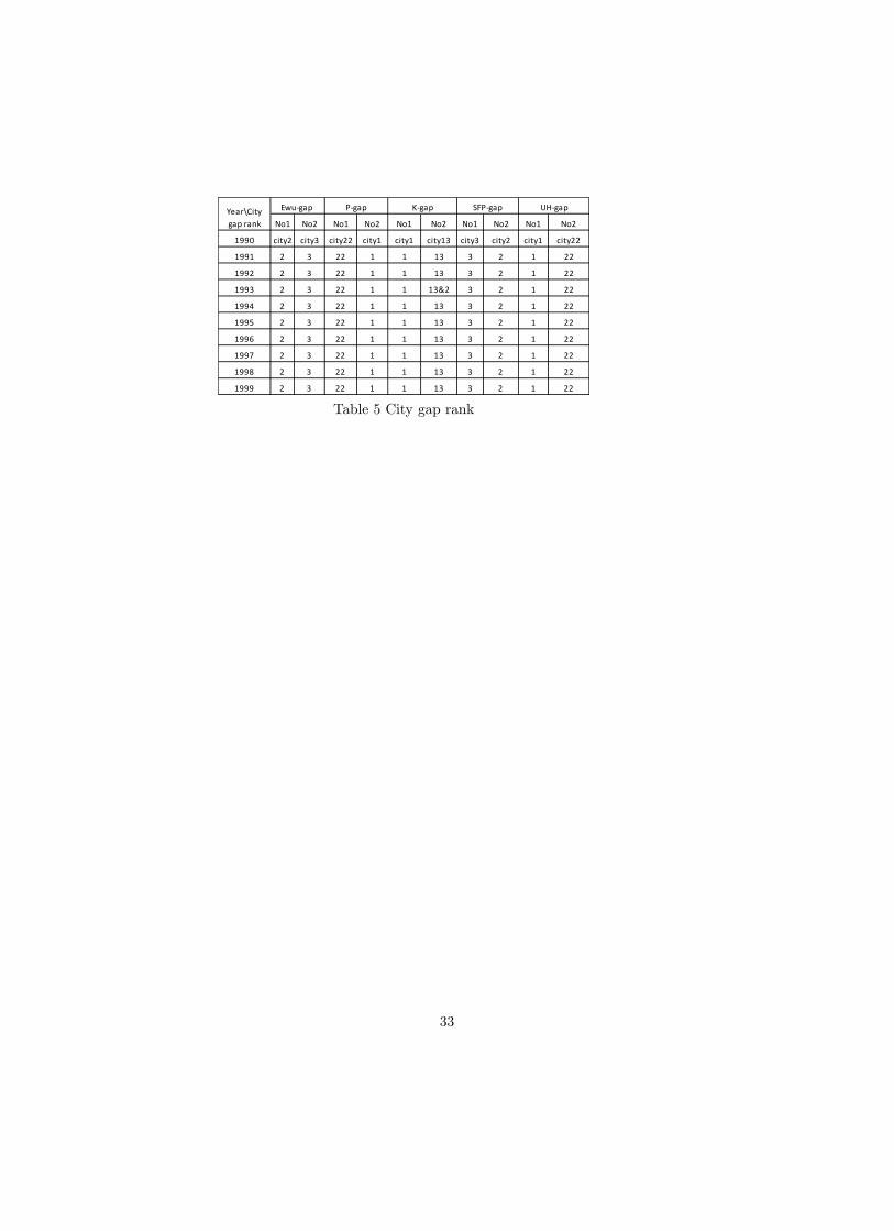
The ranking of cities by the migration factors is a crucial determinant of net

�ows but this ranking may not be the same in each year. It is evident from the

theory that at any time migration should be into cities ranked top on some life

style factor from all other cities, to some extent into cities ranked second (here it

is low quality of life inhabitants from the top ranked city who move to the second

city) and then net emigration driven by a factor where the mover currently is

in neither the top or second city. For each year and migration factor, the table

shows the cities which are ranked top and second by that particular migration

18

factor. For example in 1990 city 2 (Shenzhen) is ranked top for expected income

and city 3 (Zhuhai) is ranked second.


From this table it is evident that there is little variation in the top two rank-

ing cities on a given migration factor. There are also only �ve cities which �gure

in the table The implication is that we should expect to see intra-Guangdong

emigration from the remaining thirteen cities which are never ranked in the

top two on any criterion for migration but inward immigration into the ranked

cities. As against this there may be other reasons for migration between city

areas which we have omitted.

4.2 The Econometric Speci�cation

Our theory results in the mean desired level of intra-province net migration into

city i (2). For estimation we use this in the form11

NMi = Ai +�xji=1(x)Bxi f[�j 6=1(x)x1(x)Xj � x2(x)X1(x)] (3)

+�xji=2(x)[x2(x)X1(x) � x1(x)X2(x)]

��xi6=1(x);2(x)x1(x)Xig

This has the interpretation of a gaps model (Zhu,2002) in a multi area and

multivariate context12 . The number of coe¢ cients to estimate is 18 � 6 = 108

where 18 corresponds to the number of cities and 6 to the 5 migration criteria

11Limited degrees of freedom and lack of data on cost e¤ects impose this approximation.12 Instead of thinking of the distribution of the factor within a city, this can be interpreted

as saying for example that net (and gross) migration from a city ranked three or lower intothe top city is the total factor gain from the lower rank city achieving the mean factor of thetop city.We can also identify the constant term with a combination of a constant net migration �ow

unrelated to the gaps (giving a positive Ai) and a moving cost e¤ect which deters some of thenet migration driven by the gaps(giving a negative Ai):

19

plus a constant term for each city (detailed de�nition of the dependent variable

and regressors is in the appendix).

Further choices concern measurement of the migration driving forces.We

cannot observe the pro�ts of the selfemployed �j : However these will depend on

the demand for their services and other cost determining variables. We proxy

these by a linear function of the population size and level of capital stock in each

city, Pj ;Kj : Self employed pro�ts should be increasing in both these variables on

demand grounds and so on this count the top ranked city is that with the highest

capital stocks and population. However capital stock also plays a role in the

key three employing sectors. If capital and labour are complements, an increase

in the capital stock should raise the marginal product of labour and hence raise

the expected income variable. On the other hand if they are substitutes then

an increase in the capital stock reduces the demand for labour but raises the

productivity of the remaining workers in most cases (eg with a Cobb-Douglas

production function). Machines wipe out jobs but can raise wages. Here the

capital stock has a negative impact on migration. As for the marriage motive,

we take the stock of single females in a city to proxy the motivation of single

females who wish to migrate there to improve their marriage chances. There is

evidence that this together with the availability of jobs for females in the textile

industry are factors which cause female migration, (Fan (2003) �nds that most

female migrants work either in textiles as seamstresses or knitters or in domestic

service or assembly line type factory jobs. Huang (2001) �nds similar results

with the addition of waitressing). With respect to the urban infrastructure, we

measure this by the number of urban hukous issued. This measures the degree

of industrialisation of the area.

20

Having de�ned the rankings of cities such that the top ranked is the most

desirable, and individuals move when possible to the top two ranking cities, all of

the coe¢ cients �xi should be positive. There is some possible ambiguity with the

single female city di¤erences since it could be either a proxy for the availability

of female worker jobs especially in the textile industries or as a factor which

a¤ects marriage chances. Similarly, depending on whether capital and labour

are substitutes or complements, capital stock can have an ambiguous e¤ect on

employment prospects. Finally, population can have an ambiguous e¤ect, it

could re�ect disadvantages due to congestion in an area or the level of demand

for the services and output of the self employed.

We add a disturbance "it which is assumed to have a zero mean at each it and

initially for given i; to be independent over time t with a constant covariance

matrix across cities. We test the lack of autocorrelation of the residuals following

estimation using Wooldridge�s (2002) panel serial correlation test.

Adding the disturbance and using more succinct notation, (3) becomes

NMit = Ai +�xji=1(x)Bxi Gap

xit + "it; E"it = 0; E"it"js = �ij for all t; s

where (details of the gaps are de�ned in the appendix).

Gapit = �j 6=1(x)x1(x)Xj � x2(x)X1(x) if i = 1(x)

= x2(x)X1(x) � x1(x)X2(x) if i = 2(x)

= �x1(x)Xi if i 6= 1(x); 2(x)

Secondly we have to specify the covariance structure between cities. For each

city the variance is constant over time since it is iid. But the variances could

di¤er between cities, e¤ectively giving a panel structure to the disturbances. The

shocks of any two cities may be correlated, eg if there is some uncertainty over

21

the best destination for a migrant who has decided to move within Guangdong,

the shocks could be negatively correlated. But a global shock, like a random

change in the tightness with which hukou restrictions are imposed, could lead

to positive correlation. The nature of cross section dependence of net migration

is tested by applying the method of Peseran(2004) and de Hoyo and Sara�dis

(2006). The test statistic for this has an approximate normal distribution which

should be valid even in small samples.

We estimate the parameters by GLS allowing for the variances of distur-

bances to di¤er by city. In order to check the robustness of GLS, we also estimate

by weighted OLS and �nd equivalent results. We allow the constant terms (Ai)

and all the slope coe¢ cients Bxi to vary by city through the use of dummy vari-

ables for each city (without a common constant term). The most general model

has 107 regression parameters, which has a loglikelihood of 77:45, a Wooldridge

serial correlation statistic F (1; 17) = 4:097 (p value :059) and cross section de-

pendence test statistic of �1:12 with a p value of :261. Taken together there

is no evidence of panel e¤ects and heteroscedasticity in the disturbances, so we

use a diagonal covariance matrix of the form E"it"js = 0 for all t; s and i 6= j

but Eu2it = �2i for all t:

This regression has many insigni�cant coe¢ cients and we sequentially test

down to our base model which has 67 coe¢ cients and a log likelihood of 54:66.

It has no evidence of serial correlation, (F (1; 17) = 2:531 with a p value of 0:13):

Similarly, from the Pesaran test it has no evidence of cross city correlation (test

statistic �:70 with a p value of :486). A likelihood ratio test of this model against

the general case with 107 coe¢ cients is also easily accepted, despite our small

sample situation, �2(41) = 45:6 which has a p value of :287: So we accept this

22

base model as a �rst representation of intercity net migration in Guangdong.

Estimating the same model by weighted OLS (allowing for disturbance variances

to vary by city) gives very similar coe¢ cients, an R2 = :959 and Ramsey Reset

test statistic of F (3; 73) = :33 which is far from signi�cance with a p value of

:80. The weighted OLS residuals also show no sign of autocorrelation with a

Wooldridge test statistic of F (1; 17) = 2:79 and also no sign of cross section

dependence (the Peseran test has a p value of :451). So the evidence is that

the base model is an adequate speci�cation of the process. The accompanying

plots show the relation between the actual and predicted net migration by city

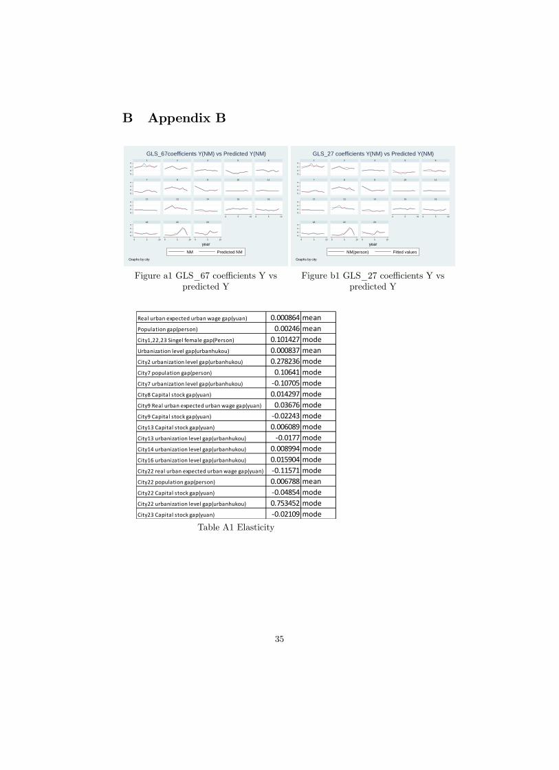
(Figure a1 and b1 in the appendix). Generally the model is replicating the data

as one would expect smoothing some of the sharper �uctuations especially in

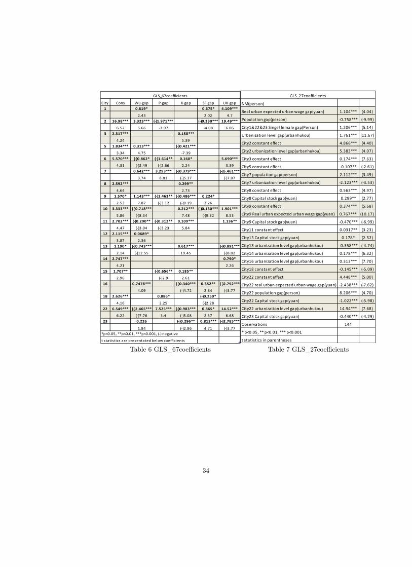
cities 1; 8; 22: The estimated coe¢ cients arranged by city and gap are shown in

the table 6 below.


Inspecting these, most coe¢ cients are very similar across cities but there are

some outlying gap-city combinations. This suggests that we may be able to test

further for equality of coe¢ cients between groups of gaps and cities. In fact,

following this strategy, we �nd a candidate model involving large simpli�cation

on our base model with just 27 coe¢ cients (table 7).


In this reduced model all cities except for 9 and 22 have a common positive

e¤ect of expected wage di¤erences. The expected wage gap does a¤ect net

migration into cities 9,22 but to a smaller extent than in the other cities. Only

23

a few cities have a responsiveness of net migration to the level of capital stock

(cities 8,9, 13,22 and 23) and in these cities there are heterogeneous reactions to

capital stock. The population gap is important in a¤ecting net migration in all

cities but only the e¤ects in cities 7 and 22 are positive e¤ect and heterogeneous

whereas in the other 16 cities the response to the gap is negative although

quantitatively small. All cities have net migration e¤ects of their degree of

urbanisation, this is an equal e¤ect in 12 cities but there are heterogeneous

e¤ects in 6 cities ( cities 2,7,13,14,16 22). The e¤ect of the gaps is thus common

for most cities and most gaps.

Generally the gaps work in a way that is consistent with the theory: the

population gap is a broad exception but it�s role generally is dominated by city

22 which is very much larger than the other cities in terms of population. There

are some other speci�c exceptions like the negative impact of the urbanisation

gap on net migration into cities 7 and 13. Most of the heterogeneous gap e¤ects

can be explained in terms of special city characteristics. City 2 has been one the

fastest growing cities in terms of capital stock and net migration. It is high urban

wage, densely populated and highly urbanised. City 7 is a northern mountainous

city with low urban wage and urbanisation, high population but low population

density and low capital stock. It shows high emigration. City 8 has a relatively

high capital stock and low population and its textile industry base does not

yield very high expected urban income, nevertheless it attracts immigration.

City 9 is a coastal city and is the main Guangdong seafood producer with other

industry concentrated on shipping construction. It is a low population and

population density city with a low expected urban income and low capital stock

but despite this it has mean positive net migration. Foshan (13) is one of the

24

industrial tigers with high expected urban income, capital stock and population

and a relatively high degree of urbanisation. It attracts positive net migration

but is neither the leading nor second city in terms of the gap rankings. Cities

14 and 16 are low expected urban wage, relatively rural cities with low capital

stock and average to low population density. Their mean net migration is close

to zero. The merged city 22 stands out as having the greatest number of speci�c

heterogeneity in the migration response to gaps. As stated above it dominates

the other cities in population size but is relatively nonurbanised although it has

a high population density. It also has low capital stock and at best average

expected urban income. It�s mean net migration is close to zero. Finally city

23 is a similar administratively merged city, sharing many of the characteristics

of city 22.

The city speci�c constant terms in Table 7 re�ect a relatively constant stream

of net migration which is not determined by the operation of the gaps. These

e¤ects are important in half of the cities and in the majority of these cities there

is inward migration which is not related to the gaps that we have identi�ed.

Comparing the plots of the actual and predicted values by city for the 27 and

67 coe¢ cient models reveals that we lose relatively little in terms of goodness

of �t from imposing these restrictions on the 67 coe¢ cient base model. We still

track the data quite well and pick up most turning points in the net migration

data. Diagnostic tests validate the assumptions that we have made on no cross

section dependence (the Peseran statistic N(0; 1) = �0:59 has a p value of :55

) and at the 5% level there is no evidence from the Wooldridge panel data test

of any autocorrelation (test statistic F (1; 17) = 3:55 and p value :08).

For the sake of robustness we also estimate the 27 coe¢ cient model by

25

weighted least squares with weights being the estimated standard deviations of

residuals for each city (so there is cross section heteroscedasticity but no cross

section dependence). We include a constant term to allow the conventional cal-

culation of R2: The coe¢ cient estimates and standard errors are very similar for

weighted least squares or panel based GLS. The R2 from weighted least squares

is :841 and running a Ramsey Reset test gives a test statistic F (3; 113) = 0:64

which has a p value of 0:59: Thus the weighted least squares indicates no model

mispeci�cation.

The loglikelihood of the 27 coe¢ cient model is �29:26: On an asymptotic

�2 test the restrictions involved would be rejected against the 67 or the 107

coe¢ cient models which had log likelihoods of 54:66 and 77:45 respectively.

However it is well known that in small sample situations the likelihood ratio

test tends to reject much too frequently (Italianer (1985)). A relatively simple

small sample correction to the likelihood ratio is provided by Anderson (1958)

( The correction is (T � q � 2(r + 1))=T ) where, in our panel context, T is the

number of time-city observations used (T = 144), q is the number of unrestricted

coe¢ cients and r the number of restrictions. Applying this correction factor to

testing the 27 coe¢ cient model against the base model gives a small sample

corrected test statistic of 20:14 which is �2( 40) then the 27 coe¢ cient model

is easily accepted. Similarly testing the 27 coe¢ cient model against the 107

coe¢ cient model with the Anderson small sample correction, it is again easily

accepted. The degree of goodness of �t (evidenced in the R2 of :841 and the

residual plots by city) is impressive for a quite parsimonious equation.

Since we have scaled the regressors to have zero mean and unit variance

across the whole sample, the estimated coe¢ cients are largely independent of

26

the units in which we measure variables. It also means that elasticities evaluated

at the mean are less relevant. For the sake of completeness we include a table

(A1) of elasticities in the appendix. We mainly compute elasticities at the mode

except where the regressor has multiple modes. The elasticities are all below

unity and very small and as expected most of them are positive. The marriage

e¤ect has the largest value for those cities in which it is a factor.

Finally there is an argument that there may be some endogeneity in the

regressors especially in the wage gap variable. Shocks in net migration may

feedback through the city labour market into shocks in the real wage. Thus

the wage gap variables may be correlated with the net migration disturbances.

We instrument the three wage gap variables by FDI and employment for the

common group of cities and for cities 9 and 22; giving 6 instruments in all (

the Sargan test for overidenti�cation has a p value of 0:265) and perform a

Hausman-Wu test of the di¤erence between the IV and the OLS estimates. It

is not signi�cant (the p value is 0:42); and so we conclude that there are no

signi�cant feedback e¤ects between net city migration and the city wage gap

variable.

5 Conclusions

Guangdong has been one of the fastest growing regions within a rapidly growing

and changing China. Some of the initial impetus came from central government

initiatives but then decentralised market forces also came into play. One of these

is the movement of people between the prefecture-level divisions of Guangdong.

On the basis of data covering the period 1990-99, we analyse this movement

using a structural economic model in the tradition of Harris-Todaro and Krug-

27

man. Our approach allows for di¤ererentials in �ve city characteristics: real

wage, population and capital stock, urbanisation and marriage opportunities

between the 18 the prefecture-level cities under the administration of Guang-

dong province. Earlier research has also identi�ed some of these factors but

lacked an integrated framework. Our results �nd the causal links and quantita-

tive importance of multiple migration determinants. We analyse theoretically

how city characteristics should impact on inter-city net migration and then, af-

ter understanding the data, estimate the parameters in the migration process

econometrically allowing for cross section heteroscedasticity.

There are some theoretical innovations. Our approach allows for multivari-

ate determinants and multi-location choices of net migration �ows. People move

to places where the chance of an improvement of their current circumstances

in some dimension is highest. We con�rm the basic Harris-Todaro insight that

expected labour income di¤erences are important but also con�rm Krugman�s

view that each location has a variety of push and pull factors determining mi-

gration.

We �nd that net migration into the majority of cities can be well explained

by a common set of parameters. There is some limited heterogeneity between

cities in how net migration responds to the di¤erentials, out of a total of 90

city-di¤erential heterogeneities (= 5 � 18) we �nd that we need just 15 speci�c

coe¢ cients. The only heterogeneities are di¤erences being in the impacts of

capital stock and degree of urbanisation. Nearly half of the cities share a com-

mon mean amount of net migration which is unrelated to the �ve di¤erentials

we identi�ed. No cross section dependence and serial correlation are detected in

the �nal model. In terms of goodness of �t and tracking the data city by city,

28

our model performs well and there is no evidence of model misspeci�cation.

It is well known that Chinese labour migration is substantial and exhibits

di¤erent types of �ows. It is widely argued to be a very important component

in rapid Chinese growth and development, thus its policy importance is clear.

Although the data sources are much more abundant than 20 years ago, there

is still a paucity of degrees of freedom and coverage of some of the relevant

factors. This forces some imperfection in our modelling strategy, but, given

this, the results here are robust to a range of speci�cation tests.

References

[1] Ateno, S.K (1979), China�s special economic zones: experimental units fo

reconomic reform. Beijing Review,

[2] Chan, K. W. & Zhang, L., (1999) The hukou system and rural-urban mi-

gration in China: processes and changes. The China Quarterly, no. 160.

pp. 818-855. http://www.jstor.org/stable/656045

[3] Fan C. (1996), Economic Opportunities & Internal Migration: a Case Study

of Guangdong, The Professional Geographer, vol. 48, no.1, pp.28-45

[4] Fan C. (1999), Migration in a socialist transitional economy: heterogeneity,

socioeconomic and spatial characteristics of migrants in China and Guang-

dong Province. International Migration Review, Vol.33, No.4, pp.954-987

[5] Fan C.,(2002), Marriage & Migration in Transitional China: a Case Study

of Gaozhu, western Guangdong, Environment & Planning A, 34, 619-638

[6] Fan C., (2003), Rural-urban migration and gender division of labour in

transitional China, International Journal of urban and regional research

29

[7] Guangdong Statistical Yearbook 1990-1999, Statistical Bureau of Guang-

dong. China Statistics Press.

[8] Huang (2001), Gender, hukou and occupational attainmnet of female mi-

grants in China, Environment & Planning, vol.33, pp.257-279.

[9] Harris J.R. et M. P. Todaro (1970), �Migration, Unemployment And Devel-

opment : A Two-Sector Analysis�, American Economic Review, 60, pp.126-

4.

[10] Harris,C. (1954) The market as a factor in the localization of industry in

the United States, Annuals of the Association of American Geograpphers,

64,pp.315-348.

[11] Italianer A, (1985), A Small Sample Correction for the Likelihood Ratio

Test, Economics Letters ,19,35-317

[12] Krugman, P (1992), A dynamic spatial model. National Bureau of Eco-

nomic Research.

[13] Myrdal, G. (1957), Economic theory and uncerdeveloped regions, London:

Duchworth.

[14] Peseran H, (2006), Estimation & Inference in Large Heterogeneous Panels

with Multifactor error Structure, Econometrica, 74,4,967-1012

[15] Poncet , S (2006), Provincial migration dynamics in China: Borders, costs

and econometric motivations. Regional science & urban economics, 36, 385-

398.

[16] RUMICI, Rural-Urban Migrant Project Census Manual, 2007,

http://rse.anu.edu.au/rumici/pdf/Census%20manual_China_English08.pdf

30

[17] Todaro M., (1969), A Model of Labour Migration and Urban Unemploy-

ment in Less Developed Countries, American Economic Review, 59(1), 138-

148

[18] Renard M., Z Xu & N Zhu(2011), Migration, Urban Population Growth

& Regional Disparity in China, CERDI, Etudes et Documents, E 2007.30,

http://hal.archives-ouvertes.fr/docs/00/55/69/81/PDF/2007.30.pdf

[19] Wooldridge, J. M. 2002. Econometric Analysis of Cross Section and Panel

Data. Cambridge, MA: MIT Press.

[20] Zhu N.,(2002). The Impacts of Income Gaps on Migration Decisions in

China, China Economic Review, 13,213-230

[21] Zhu N., C Batisse & Q Li 2009,The �ow of �peasant-workers� in

China since the economic reform :a longitudinal and spatial analysis,

http://www.cerdi.org/uploads/sfCmsContent/html/317/Zhu_Batisse.pdf

A Appendix A

Figure 1 Map of Guangdong

050

,000

1000

0015

0000

1 2 3 5 6 7 8 9 10 11 12 13 14 15 16 18 22 23

Mean value of immigration, emigration and net migration

Immigration EmigrationNet migration

Figure 2 Mean value of IM, EM and NM

31

City

RealWu

(yuan)

RealWr

(yuan)

UrbanHukou/

P

Latemarriage

rate(%)

K/P(1000yu

an)

SingleFemale(million)

Population(million)

City size(millionm squ)

Guangzhou1 1.49 0.84 0.61 78.51 7.11 1.90 6.40 7.26

Shenzhen2 1.62 0.62 0.74 82.21 36.55 0.22 0.94 2.05

Zhuhai3 1.56 0.80 0.61 81.96 20.96 0.17 0.61 1.65

Shaoguan5 1.20 0.90 0.34 75.20 2.03 0.93 2.90 18.38

Heyuan6 1.28 0.83 0.18 60.72 0.61 0.97 2.90 15.48

Meizhou7 1.29 1.05 0.17 45.20 0.78 1.39 4.60 15.93

Huizhou8 1.31 0.81 0.30 75.67 4.47 0.81 2.50 10.66

Shanwei9 1.40 0.93 0.23 68.16 0.60 0.78 2.50 5.17

Dongguan10 1.34 0.62 0.25 73.78 10.27 0.47 1.40 2.47

Zhongshan11 1.44 0.70 0.28 76.07 6.48 0.37 1.20 1.80

Jiangmen12 1.31 0.86 0.33 79.48 3.57 1.12 3.70 9.44

Foshan13 1.41 0.94 0.41 72.93 8.48 0.95 3.10 3.87

Yangjiang14 1.36 1.05 0.24 68.51 0.68 0.71 2.40 7.81

Zhanjiang15 1.14 0.83 0.22 76.11 1.24 1.91 6.00 12.49

Maoming16 1.25 1.12 0.16 64.32 0.95 1.74 5.70 11.45

Qingyuan18 1.24 0.74 0.18 68.91 0.93 1.17 3.60 19.02

Mergedcity22 1.37 0.88 0.23 72.36 1.88 3.44 11.00 10.28

Mergedcity23 1.37 0.96 0.24 57.39 1.59 1.82 5.90 22.84

Table 1 Average value of key variables

Year

Real

Wu

(yuan)

Real

Wr

(yuan)

Urban

Hukou

/P

Late

marriage

rate(%)

K/P(1000

yuan)

Single

Female

(million)

Population

(million)

1990 0 0 0.56 . 1.29 0.68 0.69

1991 0.04 0.10 0.56 0.22 1.36 0.68 0.67

1992 0.06 0.11 0.57 0.19 1.42 0.67 0.70

1993 0.09 0.18 0.54 0.18 1.45 0.68 0.68

1994 0.07 0.19 0.53 0.19 1.51 0.69 0.69

1995 0.08 0.20 0.53 0.14 1.54 0.66 0.67

1996 0.11 0.22 0.53 0.11 1.55 0.69 0.67

1997 0.13 0.24 0.51 0.10 1.58 0.69 0.70

1998 0.16 0.26 0.52 0.11 1.65 0.69 0.69

1999 0.17 0.28 0.51 0.10 1.62 0.71 0.72

Table 2 Inequality between cities overtime (coe¢ cient variation of key

variables)

City NM Wgap Pgap Kgap SFPgap UHgap

Guangzhou1 2.39 0.80 0.27 2.49 0.37 4.05

Shenzhen2 1.37 3.80 0.03 1.30 0.99 0.02

Zhuhai3 0.11 0.01 0.03 0.02 3.01 0.02

Shaoguan5 0.91 0.20 0.22 0.16 0.18 0.18

Heyuan6 0.04 0.11 0.28 0.20 0.19 0.22

Meizhou7 0.79 0.17 0.43 0.32 0.27 0.35

Huizhou8 0.71 0.16 0.20 0.15 0.16 0.16

Shanwei9 0.06 0.12 0.22 0.16 0.15 0.17

Dongguan10 0.48 0.07 0.12 0.09 0.09 0.10

Zhongshan11 0.40 0.07 0.10 0.08 0.07 0.08

Jiangmen12 0.41 0.26 0.28 0.21 0.22 0.23

Foshan13 0.59 0.26 0.21 0.11 0.18 0.17

Yangjiang14 0.84 0.12 0.21 0.15 0.14 0.17

Zhanjiang15 0.23 0.27 0.54 0.39 0.37 0.43

Maoming16 0.28 0.20 0.55 0.40 0.34 0.44

Qingyuan18 0.72 0.14 0.34 0.25 0.23 0.27

Merged city22 0.26 0.54 4.01 0.72 0.67 0.63

Merged city23 0.32 0.30 0.52 0.38 0.35 0.41

Table 3 Mean value of regressionvariables among di¤erent cities

Year NM EWugap Pgap Kgap SFPgap UHgap

1990 1.136 1.7E+08 9.26E+07 1.38E+08 5.76E+08 1.32E+08

1991 1E+09 7.34E+07 4.92E+08 1.55E+08 7.43E+07

1992 1.2E+08 9.61E+08 7.19E+07 5.65E+07 8.52E+07

1993 1.593 3.1E+07 1.68E+09 1.58E+02 1.46E+08 8.69E+07

1994 2.080 2.3E+08 1.88E+08 9.27E+08 5.13E+07 1.35E+08

1995 1.874 4.1E+07 9.44E+08 1.20E+08 1.28E+08 1.40E+08

1996 1.208 2.5E+08 1.40E+08 1.84E+08 5.80E+07 2.24E+08

1997 1.371 5E+07 6.12E+08 8.41E+07 7.40E+07 2.98E+08

1998 1.143 1.5E+08 1.07E+09 7.16E+07 1.92E+08 1.79E+08

1999 1.805 4.6E+07 1.24E+08 6.49E+07 1.26E+08 5.27E+07

Table 4 Inequality between cities over time(coe¢ cient variation)

32

No1 No2 No1 No2 No1 No2 No1 No2 No1 No2

1990 city2 city3 city22 city1 city1 city13 city3 city2 city1 city22

1991 2 3 22 1 1 13 3 2 1 22

1992 2 3 22 1 1 13 3 2 1 22

1993 2 3 22 1 1 13&2 3 2 1 22

1994 2 3 22 1 1 13 3 2 1 22

1995 2 3 22 1 1 13 3 2 1 22

1996 2 3 22 1 1 13 3 2 1 22

1997 2 3 22 1 1 13 3 2 1 22

1998 2 3 22 1 1 13 3 2 1 22

1999 2 3 22 1 1 13 3 2 1 22

Ewugap Pgap Kgap SFPgap UHgapYear\Citygap rank

Table 5 City gap rank

33

City Cons Wugap Pgap Kgap SFgap UHgap

1 0.819* 0.675* 4.109***

2.43 2.02 4.7

2 16.98*** 3.323*** ()1.971*** ()0.230*** 19.49***

6.52 5.66 3.97 4.08 6.06

3 2.317*** 0.158***

4.24 5.39

5 1.834*** 0.313*** ()0.421***

3.34 4.75 7.39

6 5.570*** ()0.862* ()1.614** 0.160* 5.690***

4.31 ()2.49 ()2.66 2.24 3.39

7 0.642*** 3.293*** ()0.379*** ()5.461***

3.74 8.81 ()5.37 ()7.07

8 2.592*** 0.299**

4.64 2.73

9 1.570* 1.143*** ()1.463** ()0.486*** 0.224*

2.53 7.87 ()3.12 ()9.19 2.26

10 3.333*** ()0.718*** 0.212*** ()0.130*** 1.901***

5.86 ()8.34 7.48 ()9.32 8.53

11 2.702*** ()0.290** ()0.312** 0.109*** 1.136**

4.47 ()3.04 ()3.23 5.84

12 2.115*** 0.0689*

3.87 2.36

13 1.190* ()0.743*** 0.617*** ()0.891***

2.14 ()12.55 19.45 ()8.02

14 2.747*** 0.790*

4.21 2.26

15 1.707** ()0.656** 0.185**

2.96 ()2.9 2.61

16 0.7478*** ()0.340*** 0.352** ()2.792***

4.09 ()4.72 2.84 ()3.77

18 2.626*** 0.886* ()0.250*

4.16 2.25 ()2.28

22 6.549*** ()2.465*** 7.525*** ()0.983*** 0.865* 14.52***

6.22 ()7.76 3.4 ()5.08 2.37 6.68

23 0.226 ()0.296** 0.813*** ()2.785***

1.84 ()2.86 4.71 ()3.77*p<0.05, **p<0.01, ***p<0.001, () negative

t statistics are presentated below coefficients

GLS_67coefficients

Table 6 GLS_67coe¢ cients

NM(person)

Real urban expected urban wage gap(yuan) 1.104*** (4.04)

Population gap(person) 0.758*** (9.99)

City1&22&23 Singel female gap(Person) 1.206*** (5.14)

Urbanization level gap(urbanhukou) 1.761*** (11.67)

City2 constant effect 4.866*** (4.40)

City2 urbanization level gap(urbanhukou) 5.383*** (4.07)


City5 constant effect 0.107** (2.61)

City7 population gap(person) 2.112*** (3.49)



City8 Capital stock gap(yuan) 0.299** (2.77)


City9 Real urban expected urban wage gap(yuan) 0.767*** (10.17)

City9 Capital stock gap(yuan) 0.470*** (6.99)

City11 constant effect 0.0317** (3.23)

City13 Capital stock gap(yuan) 0.178* (2.52)






City22 real urban expected urban wage gap(yuan) 2.438*** (7.62)

City22 population gap(person) 8.206*** (4.70)




Observations 144

* p<0.05, ** p<0.01, *** p<0.001

t statistics in parentheses

GLS_27coefficients

Table 7 GLS_27coe¢ cients

34

B Appendix B2

02

42

02

42

02

42

02

4

0 5 10 0 5 10

0 5 10 0 5 10 0 5 10

1 2 3 5 6

7 8 9 10 11

12 13 14 15 16

18 22 23

NM Predicted NM

year

Graphs by city

GLS_67coefficients Y(NM) vs Predicted Y(NM)

Figure a1 GLS_67 coe¢ cients Y vspredicted Y

20

24

20

24

20

24

20

24

0 5 10 0 5 10

0 5 10 0 5 10 0 5 10

1 2 3 5 6

7 8 9 10 11

12 13 14 15 16

18 22 23

NM(person) Fitted values

year

Graphs by city

GLS_27 coefficients Y(NM) vs Predicted Y(NM)

Figure b1 GLS_27 coe¢ cients Y vspredicted Y

Real urban expected urban wage gap(yuan) 0.000864 meanPopulation gap(person) 0.00246 meanCity1,22,23 Singel female gap(Person) 0.101427 modeUrbanization level gap(urbanhukou) 0.000837 meanCity2 urbanization level gap(urbanhukou) 0.278236 modeCity7 population gap(person) 0.10641 modeCity7 urbanization level gap(urbanhukou) 0.10705 modeCity8 Capital stock gap(yuan) 0.014297 modeCity9 Real urban expected urban wage gap(yuan) 0.03676 modeCity9 Capital stock gap(yuan) 0.02243 modeCity13 Capital stock gap(yuan) 0.006089 modeCity13 urbanization level gap(urbanhukou) 0.0177 modeCity14 urbanization level gap(urbanhukou) 0.008994 modeCity16 urbanization level gap(urbanhukou) 0.015904 modeCity22 real urban expected urban wage gap(yuan) 0.11571 modeCity22 population gap(person) 0.006788 meanCity22 Capital stock gap(yuan) 0.04854 modeCity22 urbanization level gap(urbanhukou) 0.753452 modeCity23 Capital stock gap(yuan) 0.02109 mode

Table A1 Elasticity

35

Description of key variables

Wu

wuit =average wage index in top three unitsi;t

CPI indexi;twhere, average wage index in top three unitsi;t =

average wage in top three unitsi;taverage wage in top three unitsi;t=0and; CPI indexi;t=

CPIi;tCPIi;t=0

wui =9Pt=0wui;t (�)

i = 1:::18; t = 0:::9

wr

wri;t =gross average rural income indexi;t

CPI indexi;twhere; gross average rural incomei;t =

gross rural primary industry ouputi;trural primary industry labor fore

and, gross average rural income indexi;t =gross average rural incomei;tgross average rural incomei;t=0and; CPI indexi;t=

CPIi;tCPIi;t=0

wri =9Pt=0wri;t (�)

i = 1:::18; t = 0:::9

UH rate

urban hukou ratei;t=urban hukou populationi;t

city populationi;t

urban hukou ratei =9Pt=0urban hukou ratei;t (�)

i = 1:::18; t = 0:::9

Lmar-rateLate marriage ratei;t is the ratio of the number of

females who were at least 23 years old atmarriage to the total number of frist marriages.

K/P

(K/P)i;t =capital stock i;t

city populationi;t;

capital stock i;t = Ki;t = (1� �)Ki;t�1 + FDIi;t;

where � is depreciation rate.� =

originalKi;t=1992�netKi;t=2

originalKi;t=2

i = 1:::18; t = 0:::9

SFP

number of single femalei;t =number of femalei;t�number of married and child

bearing agei;t:where, child bearing age is between 20-49 years old

i = 1:::18; t = 0:::9

36

Descirption of esimated variablesNM Number of net migrants

Ewu-gap

If i=1(x), expected urban wage1(x) �Purban huouj

�expected urban wage2(x)�urban huou 1(x)If i=2(x), expected urban wage2(x)�urban huou1(x)

�expected urban wage1(x)�urban huou 2(x)If i=3(x), -expected urban wage1(x)�urban huouj(x);

j=1...18, i 6= j;1(x) stands for the highest expected urban wage city

P-gap

If i=1(x), city population1(x) �Pargilculture huouj

�city population2(x)�agriculature hukou 1(x)If i=2(x), city population2(x)�agricultural hukou1(x)

�city poplation1(x)�argiculture hukou 2(x)If i=3(x), -city population1(x)�argiculturehukouj(x)

j=1...18, i 6= j;1(x) stands for the biggest city population city

K-gap

If i=1(x), capital stock1(x) �P

jagricultural hukou

�capital stock2(x)�argiculture hukou1(x)If i=2(x), capital stock2(x)�agricultural hukou1(x)

�capital stock1(x)�argiculture hukou 2(x)If i=3(x), -capital stock1(x)�argiculturehukouj(x)

j=1...18, i 6= j;1(x) stands for the largest amount of capital stock city

SFP-gap

If i=1(x), single female1(x) �Psingle femalej

�single female2(x)�single female 1(x)If i=2(x), single female2(x)�single female1(x)

�capital stock1(x)�single female2(x)If i=3(x), -single female1(x)�single femalej(x)

j=1...18, i 6= j;1(x) stands for the smallest number of single female city

UH-gap

If i=1(x), urban hukou1(x) �Pargilculture huouj

�huban hukou2(x)�agriculature hukou 1(x)If i=2(x), urban hukou2(x)�agricultural hukou1(x)

�urban hukou1(x)�argiculture hukou 2(x)If i=3(x), -urban hukou1(x)�argiculturehukouj(x)

j=1...18, i 6= j;1(x) stands for the biggest number of urban hukou city

37