Embed Size (px)
Citation preview
Economics Department
Discussion Papers Series ISSN 1473 – 3307
CORRUPTION AROUND THE WORLD:
EVIDENCE FROM A
STRUCTURAL MODEL
Axel Dreher, Christos Kotsogiannis and Steve McCorriston
Paper number 07/02
URL: http://business-school.exeter.ac.uk/economics/papers/
DISCUSSION PAPERS IN ECONOMICS
ISSN 1473 – 3307
UNIVERSITY OF EXETER
DEPARTMENT OF ECONOMICS
Paper number 07/02
Axel Dreher,a Christos Kotsogiannis
b and Steve McCorriston
b
July 2007
Abstract
The causes and consequences of corruption have attracted much attention in recent
years by both academics and policy makers. Central in the discussion on the impact of
corruption are perception-based indices. Recent research has shown that perceived
corruption might not be a good indicator of actual corruption in a country. In this
paper, we employ a structural equation model—that treats corruption as a latent
variable that is directly related to its underlying causes and effects—to derive an
index of corruption. The index of corruption is derived for approximately 100
countries over the period 1976-97.
Keywords: Corruption; Economic Development; Latent Variables; Structural
Equation Models.
JEL: H10; O1; K49; C39.
aEHT Zurich, KOF Swiss Economic Institute, Weinbergstrasse 35, 8092 Zurich,
Switzerland and CESifo, Germany; E-mail: [email protected] of Economics, School of Business and Economics, University of Exeter,
Streatham Court, Rennes Drive, Exeter EX4 4PU, England, UK. E-mails:
CORRUPTION AROUND THE WORLD: EVIDENCE FROM A
STRUCTURAL MODEL∗
by
Axel Dreher,†,a Christos Kotsogiannis‡ and Steve McCorriston‡
First version: September 2006This version: June 14, 2007
Abstract: The causes and consequences of corruption have attracted much attentionin recent years by both academics and policy makers. Central in the discussion onthe impact of corruption are perception-based indices. Recent research has shown thatperceived corruption might not be a good indicator of actual corruption in a country. Inthis paper, we employ a structural equation model—that treats corruption as a latentvariable that is directly related to its underlying causes and effects—to derive an indexof corruption. The index of corruption is derived for approximately 100 countries overthe period 1976-97.
Keywords: Corruption; Economic Development; Latent Variables; Structural Equation Mod-
els.
JEL classification: H10; O1; K49; C39.
†EHT Zurich, KOF Swiss Economic Institute, Weinbergstrasse 35, 8092 Zurich, Switzer-land and CESifo, Germany; E-mail: [email protected]
‡Department of Economics, School of Business and Economics, University of Exeter,Streatham Court, Rennes Drive, Exeter EX4 4PU, England, UK. E-mails: [email protected], [email protected]
aCorresponding author.
∗Acknowledgements: The comments of two anonymous referees and Bruno Frey, ThomasHerzfeld, Johann Graf Lambsdorff, Paolo Mauro, Pierre-Guillaume Meon, Michael Pick-hardt, Jordi Sarda and Michael Smart are gratefully acknowledged. We also thankDavid de Meza and Gary Stasser for many insightful discussions. Research assistancewas ably provided by Nils Herger. Kotsogiannis acknowledges financial support fromthe Economic and Social Research Council (ESRC award L219252102) and the CatalanGovernment Science Network (Project No. SGR2005-177). All remaining errors are ofcourse ours.
1 Introduction
Corruption around the world is believed to be endemic and pervasive, a significant con-
tributor to low economic growth, to stifle investment, to inhibit the provision of public
services and to increase inequality to such an extent that international organizations like
the World Bank have identified corruption as ‘the single greatest obstacle to economic
and social development’ (World Bank, 2001).1,2 More recently, the World Bank has es-
timated that more than US$ 1 trillion is paid in bribes each year and that countries
that tackle corruption, improve governance and the rule of law could increase per capita
incomes by a staggering 400 percent (World Bank, 2004). Commensurate with the place
of corruption on the policy agenda, the economics literature has paid increased attention
to the issue.3 Recently, there have been attempts to address the causes and consequences
of corruption from an empirical standpoint. Notable efforts in this area include, among
others, Mauro (1995) on the impact of corruption on economic growth and investment,
Treisman (2000) on the causes of corruption, and Fisman and Gatti (2002) on the links
between political structure and corruption.4
Corruption is a variable that cannot be measured directly. However, in recent years,
several organizations have developed a corruption perception-based index across a wide
range of countries to qualitatively assess the pervasiveness of corruption. These indices
have been used in econometric studies (including those mentioned above) either as a
dependent variable when exploring the causes of corruption or as an explanatory variable
when investigating its consequences. Undoubtedly, these perception-based indices have
made an important contribution to the understanding of the pervasiveness of corruption
across countries. They are, however, not free of problems. One such problem refers to the
fact that these indices do not relate directly to the factors that are responsible for causing
1This argument is not supported unanimously. Routine corruption may have the desirable propertyof creating incentives for public employees. For an early statement of this argument, see Leff (1964),Morgan (1964) and Lui (1985). For a criticism of this view see Tanzi (1998), Kaufmann and Wei (1999)and Rose-Ackerman (1999). For recent empirical evidence, see Meon and Weill (2006) and Dreher andGassebner (2007).
2The definition of corruption varies widely but the most widespread one seems to be the one providedby Klitgaard (1988) that emphasizes the deviation of public officials from formal duties. As Klitgaardnotes, a corrupt official ‘deviates from the formal duties of a public role because of private-regarding(personal, close family, private clique) pecuniary or status gains; or violates rules against the exerciseof certain private-regarding behavior,’ p. 23. See also Rose-Ackerman (1999).
3Bardhan (1997), Jain (2001), and Aidt (2003) provide comprehensive accounts of the latest devel-opments on corruption. See also Rose-Ackerman (1978, 1999), Lambsdorff (1999) and Seldadyo and deHaan (2005).
4Kaufmann et al. (1999) provide a comprehensive account of empirical work on corruption.
1
corruption.5 The consequence of this may be that the correlation between perceived
corruption and actual corruption is low. Indeed, recent research has pointed precisely
to this. According to Mocan (2004) perceived and actual corruption are completely
unrelated once other relevant factors are controlled for. Similarly, Weber Abramo (2005)
shows that perceived corruption is not related to bribery. Andvig (2005) and Weber
Abramo (2005) consequently conclude that perception-based indices reflect the quality of
a country’s institutions rather than its actual degree of corruption. Svennson (2005) also
highlights problems in the construction of perception-based indices while Razafindrakoto
and Roubaud (2006) compare perception-based indices with direct surveys for six sub-
Saharan African countries and conclude that the perception-based measures do not tie
in with reality. Furthermore, according to the results of Bjørnskov (2006), the six indices
of governance (including a measure of perceived corruption) developed by Kaufmann et
al. (1999) cannot be separated statistically and, therefore, all measure one underlying
governance factor.
It is clear, then, that the provision of a meaningful and comparable estimate of corruption
across countries requires an alternative approach to the one usually taken. This paper
deals with this issue. Recognizing that corruption is inherently a latent variable, and
relying on the existing theory that identifies measurable variables that indicate and cause
corruption, we employ a structural equation methodology to estimate the relationship
between the manifest variables (causes and indicators) and the latent (corruption).6 In
particular, we estimate an index of corruption employing a special case of a structural
equation model, the Multiple Indicators Multiple Causes (MIMIC) model, introduced to
economics by Weck (1983), and Frey and Weck-Hanneman (1984) and latterly explored
by Loayza (1996), Giles (1999), and Schneider (2005), among others, to measure the size
of the hidden economy,7 Raiser et al. (2000) to investigate the institutional change in
Eastern Europe, and Kuklys (2004) to measure welfare.
Based on a sample of around 100 countries, we derive an index of corruption based
on estimated parameters that relate directly to its causes and indicators. There are
5They might also suffer from artificial ‘inertia’: once a country is reported to be corrupt, perceptionabout this country may not change, leading future survey respondents to over-estimate true corruption.Other problems exist. See, for instance, Andvig et al. (2000), Kaufmann et al. (2003), and Søreide(2005).
6As will be seen later on, the estimated model does rely on one perception-based variable but thisis unavoidable due to lack of appropriate data. Nevertheless, the structural dimension of the estimatedmodel is preserved since this perception-based index is not the only determinant that is being used. Weturn to this below.
7Schneider and Enste (2000, 2002) offer a comprehensive account of studies on the hidden economythat have employed this approach. Pickhardt and Sarda Pons (2006) provide a recent application toGermany’s shadow economy.
2
two key advantages to this approach of measuring corruption. First, the ranking of
countries in our index is firmly based on a structural relationship between causes and
the variables that are known to be good proxies (indicators) of corruption. The selection
of the variables are drawn from the existing literature on corruption. In this sense,
the methodology is confirmatory in nature in that the structural model confirms (or
otherwise) the role of the causal factors as determinants of corruption. Second, since
we have, albeit limited, data on the causes and indicators of corruption dating back to
the 1970s, we can re-estimate the model for different time periods allowing us to address
the question of whether corruption has increased or decreased since the late 1970s. In
addition, the index also has implications for empirical studies of corruption. As discussed
later, the index provides not only an ordinal ranking of corruption across countries but
it also, reflecting the nature of the data, provides a meaningful measure of ‘distance’
between countries in the corruption index.
The key results are as follows. The estimated model produces cross-countries indices (and
so a ranking) of corruption based on the structural relationship between the variables
that cause and indicate corruption from the mid-1970s to the late 1990’s. The resulting
ranking of countries is not surprising with the developed countries reported as having
lower corruption than the developing ones. The estimates show that in 1997 Switzerland
was the least corrupt country followed by Japan, Norway, Denmark, Germany and the
Netherlands. The US is in 9th position followed by France and Belgium. The most
corrupt countries are (in reverse order) Zambia, Ghana, the Central Africa Republic,
Syria, Nigeria and Guinea-Bissau, the most corrupt country.
The paper is organized as follows. In Section 2, the MIMIC methodology to measure
corruption as a latent variable is presented. In Section 3, data on the causes and indi-
cators of corruption are discussed. In Section 4, the results from the estimated MIMIC
model and the index of corruption across countries are presented, while in Section 5
we provide some further discussion on (and the use of) the derived index. Finally, in
Section 6, we conclude with some observations on the relevance of the results for further
empirical research on corruption.
2 A structural equation model for corruption
We focus on the MIMIC model that is characterized by a latent endogenous variable with
no measurement error in the independent variables. The unknown coefficients of the
model are estimated separately through a set of structural equations with the indicator
variables being used to capture the effect of the unobserved variables indirectly. Using
causal and indicator variables of corruption across countries, the structural model can
3
be estimated and, in turn, a cardinal index of corruption across countries retrieved.
More formally, but briefly,8 the specification of the MIMIC model is as follows. Let yi,
i = 1, . . . , n, be one of the indicators of the latent random variable corruption, denoted
by η, such that:
y1 = γ1 η + u1, . . . , yn = γn η + un , (1)
where γi is the factor loading9 and ui, i = 1, . . . , n, are the error terms with mean zero
and covariance matrix Θu. The disturbances are mutually independent such that any
correlation across the indicators are driven by the common factor η. Equation (1) is,
then, a confirmatory factor analysis model for the observable indicators y = (y1, . . . , yn)′
with common factor η and unique factor ui, i = 1, . . . , n. The latent variable η is
linearly determined by a set of exogenous variables (causes) given by x = (x1, . . . , xk)′
and a stochastic disturbance ǫ, that is:
η = β′x + ǫ , (2)
where β = (β1, . . . , βk)′. The model, therefore, comprises of two parts: the measure-
ment model in equation (1) which specifies how the observed endogenous variables are
determined by the latent variable and the structural equation model, equation (2), which
specifies the relationship between the latent variable and its causes.10 Since the latent
variable η is unobserved, it is impossible to recover direct estimates of the structural
parameters β. Substituting (2) into (1), the MIMIC model can be interpreted as a
multivariate regression model that takes the reduced form, connecting the observable
variables, given by:
y = Π′x + z , (3)
where the reduced-form coefficient matrix is Π = γβ′, where γ = (γ1, . . . , γn)′, and the
reduced-form disturbance vector is z = γǫ + u, with covariance matrix:
Θǫ = E[(γǫ + u)(γǫ + u)′] = γγ ′σ2
ǫ + Θu , (4)
where σ2
ǫ is the variance of the disturbance ǫ. Clearly, the rank of the reduced form
regression matrix Π, in (3), is equal to 1. The error covariance matrix Θǫ, being the
sum of a rank-one matrix and a diagonal matrix, is also similarly constrained. This prop-
erty calls for a normalization of one of the elements of the vector γ to a pre-specified
8See Joreskog and Goldberg (1975) for the original contribution to estimating the MIMIC modelwith a single latent variable and Bollen (1989) for a more accessible, but thorough, treatment.
9A factor loading represents the expected change in the respective indicators following a one unitchange in the latent variable.
10Figure 1, presented in Section 3, provides a graphical representation of the system of simultaneousequations (path diagram) estimated in this paper.
4
value prior to the estimation of the reduced form of the model. The fundamental hy-
pothesis for a structural equation model is that the covariance matrix of the observed
variables, denoted by S, may be parameterized based upon a given model specification
with parameter vector δ. The model parameters are estimated based upon minimizing
the function:11
F = ln |Σ(δ)|+ tr{SΣ−1(δ)} − ln |S| − ρ , (5)
where Σ−1 is the estimated population covariance matrix and ρ = k + n is the number
of measured variables.
Once the hypothesized relationship between the variables has been identified and esti-
mated, the latent variable scores ηj for each country j = 1, . . . J can be obtained following
the procedure suggested by Joreskog (2000). Intuitively, what the procedure behind the
derivation of latent variable scores (and so of the ranking and indices of corruption) does
is to calculate a score using the estimated coefficients for both the causal and indicator
variables placing particular weights to the individual variables. In principle, the weight
that each individual variable has is determined by minimizing an underlying objective
function relating to the statistical properties of the sample data (specifically, the mean
vector of the coefficients of the indicator variables and the covariance matrices across
the random errors relating to both the indicator and causal variables), normally putting
more weight on the indicator variables, as compared to the causal variables.12 This
process is not too dissimilar to standard uses of econometric models when used to derive
a value for the dependent variable, the difference being that, in this case, the structural
equation model uses the full information on causes and indicators and the dependent
variable is an unobserved latent, which relates directly to the causes and indicators used
to specify and estimate the model. The derived latent variable scores are, then, used to
rank countries in terms of least to most corrupt and also provide a measure of distance
between countries and, therefore, provide evidence of the extent of corruption across
countries.
Clearly, then, the challenge in implementing this framework is to identify the relationship
amongst the variables. This, together with data issues, is discussed in the following
section.
11This, of course, presumes that the observed variables have a distribution that is multivariate normal.See also footnote 22.
12The computations of the latent scores are carried out in the LISRELr software.
5
3 Causes and indicators of corruption
3.1 Causes of corruption
To identify the hypothesized variables that relate to the causes and indicators of cor-
ruption, we draw extensively on the theoretical and empirical literature on this topic.
We start with a discussion of the causal variables and then turn to the variables that
have been used as indicators. To ease the exposition, the causal variables have been
categorized into four main factor-groups namely: political and judicial factors; historical
factors; social and cultural factors, and economic factors.13
3.1.1 Political factors
The political factors capture the democratic environment of a country, the effectiveness
of its judicial system and the origin of its legal system. The role of an established democ-
racy has been highlighted in several studies of corruption (see, among others, Treisman
(2000), and Paldam (2003)). It is widely believed that corruption is related to the defi-
ciencies of the political system and that an established democracy, by promoting political
competition and hence increasing transparency and accountability, can provide a check,
albeit an imperfect one, on corruption. Other characteristics of the political environ-
ment, including electoral rules (Persson et al. (2003)) and the degree of decentralization
(Treisman (2000), and Fisman and Gatti (2002)) may also be important in explaining
corruption.14
The judicial system is also expected to play a role in controlling corruption (Becker
(1968)). The role of the legal system and the rule of law have featured prominently in
many recent studies on the quality of governance and its consequences for development
(see, for example, North (1990), and Easterly and Levine (1997)). Strong legal foun-
dations and efficient legal systems with well-specified deterrents protect property rights
and so provide a stable framework for economic activity. Failure of the legal system to
provide for the enforcement of contracts undermines the operation of the free market
and, in turn, reduces the incentives for agents to participate in productive activities.
But legal systems may differ in the degree to which property rights are protected and in
the quality of government they provide. Empirical work suggests that the common law
system, mostly found in the former colonies of Britain, appear to have better protection
13The specific data employed in our modeling effort is discussed in Section 4. Description of all thevariables that have been tried and their sources can be found in the appendix.
14To be more precise, since the measure of corruption is based on the perception-based indices dis-cussed above, these studies investigate whether the structure of the political system leads to higherlevels of perceived corruption.
6
of property rights compared with the civil law system typically associated with the for-
mer colonies of continental Europe (see, for example, La Porta et al. (1999)). Political
instability may also matter for corruption, the expectation being that more unstable
countries will have higher levels of perceived corruption.15
3.1.2 Historical factors
To a large extent, it is difficult to separate the historical factors from the political and
judicial factors since the effectiveness of the judicial system is dependent on the colonial
heritage of the country in question. La Porta et al. (1999) show that those countries
that were former colonies of Britain and who adopted the common law system appear to
have more effective judicial systems than those who adopted civil law systems associated
with former colonies of continental European countries. Treisman (2000) also explores
the direct influence of historical tradition on perceived corruption showing that former
British colonies or dominions appear to reduce perceived corruption in excess of the role
played by the common law system.
3.1.3 Social and cultural factors
This group of factors captures the social and cultural characteristics of a country that
may impact upon the pervasiveness of corruption in a given country. For example,
religion may shape social attitudes towards social hierarchy and family values and thus
determine the acceptability, or otherwise, of corrupt practices. In more hierarchical
systems (for example, Catholicism, Eastern Orthodoxy and Islam), challenges to the
status quo are less frequent than in more equalitarian or individualistic religions. The
role of the religious tradition and corruption has been explored explicitly by Treisman
(2000) who found that a Protestant tradition appears to have a negative (though small)
effect on perceived corruption. Religion may also impact on the quality of the legal
system, as explored by La Porta et al. (1999). They found that countries with a high
proportion of Catholics or Muslims reduces the quality of government and, by extension,
may reduce the deterrence of corruption. Religious fractionalization may also have an
impact on corruption and other characteristics associated with the quality of government
(Alesina et al. (2003)).
Ethnic and linguistic fractionalization of a society may also contribute to the perva-
siveness of corruption in a given country. The evidence is, however, mixed. Treisman
(2000) found no evidence that linguistic fractionalization had a direct impact on per-
ceived corruption, while La Porta et al. (1999) found evidence that, in societies that
were more ethno-linguistically diverse, governments exhibited inferior performance. More
15Treisman (2000), however, finds little support for this.
7
recently, Alesina et al. (2003) have presented evidence that ethnic and linguistic frac-
tionalization has a statistically significant impact on corruption i.e., countries that are
ethno-linguistically diverse are associated with higher perceived levels of corruption.
3.1.4 Economic factors
The economic determinants of corruption across countries have focussed typically on
three factors: the degree of openness, a country’s endowments of natural resources and
the size of the public sector. Less open countries restrict trade and impose controls on
capital flows. This creates rents and hence enhances the incentives to engage in corrupt
activities. There are a number of papers that have investigated this issue: for example,
Ades and Di Tella (1999) have shown that increased competition reduces corruption and
that more open economies are less corrupt. Treisman (2000) has shown that higher im-
ports lowers corruption. Wei and Wu (2001) have presented evidence that countries with
capital controls have higher corruption and, in turn, receive less foreign investment and
are more prone to financial crisis. More recently, Neeman et al. (2003) have shown that
the effect of corruption on economic growth depends on the openness of the economy.16
Natural resource endowments have also featured in cross-country studies of corruption;
the justification here being that the concentration of exports on natural resources is a
proxy for rent-seeking opportunities. Ades and Di Tella (1999) suggest that corruption
may offer greater gain to officials who exercise control over the distribution of the rights
to exploit these natural resources. Treisman (2000) finds that a higher concentration of
natural resource exports has a positive effect on perceived corruption.
Several studies on the causes of corruption have emphasised the size of the public sector.
Tanzi (1998), for instance, notes that the significant role of the public sector in the
economy affords public officials some degree of discretion in the allocation of goods and
services provided and hence increases the likelihood of corruption. This mechanism is
reinforced if the wages public officials receive are relatively low. This issue is explored
by van Rijckeghem and Weder (2001) who find that low wages for civil servants have a
statistically significant effect on (perceived) corruption. Treisman (2000), however, finds
rather inconclusive evidence of the size of the public sector in influencing corruption
across countries.
We now turn to a discussion of the possible indicators of the structural model.
16Neeman et al. (2003) suggest that higher levels of openness are more likely to increase the impactof corruption as openness will allow for the dissipation of stolen money abroad. However, while theyuse an overall index of openness, the mechanism for whether corruption will have this effect is primarilylimited to restrictions on the capital account.
8
3.2 Indicators of corruption
As has been the case regarding the causal variables to be used as determinants of cor-
ruption, the existing literature offers sufficient guidance with respect to appropriate
indicators. The challenge is to select variables that appear to be correlated with the
pervasiveness of corruption across the countries on our sample. This, as emphasized
above, will enable us to estimate the MIMIC model and retrieve a measure of the latent
variable. While there are a large number of candidate variables, we report only those
that were successful in our modeling effort.17
Naturally, the most obvious indicator variable that should be incorporated into the
structural model is GDP per capita. Almost all available evidence would appear to
suggest that corruption varies inversely with development (see, among others, Mauro
(1995) and Paldam (2003)). Capital control restrictions are also included as an indicator
variable. As noted in the discussion above, countries less open to foreign trade appear
to be correlated with high levels of corruption.18 More specifically, recent studies have
noted that countries appearing to exhibit relatively high levels of corruption are more
likely to impose capital account restrictions (Wei and Wu (2001) and Dreher and Siemers
(2005)). Recent empirical studies on the consequences of corruption have also focused on
the allocation of resources, emphasizing not only the negative impact of corruption on
investment but also its negative impact on the composition of investment. Mauro (1997)
argues that the allocation of public procurement contracts through a corrupt system will
lead to lower quality public services and quality of infrastructure.19 A natural variable
that captures the distortion of corruption on the allocation of resources is a measure of
financial development. One would expect, in the absence of a well-developed financial
sector, that corruption would be particularly distorting relative to those countries where
a highly developed financial sector is present. Along these lines, Hillman and Krausz
(2004) argue that corruption provides the source of the ineffectiveness of the financial
system by reducing the volume of financial intermediation. Following Claessens and
Laeven (2003), financial development is proxied by private credit as a share of GDP.
17Indicator variables that were tried, but without success, include, among others, growth of GDP,growth of GDP per capita, public investment as a share of GDP and trade as a percentage of GDP.Naturally, the size of the shadow economy may also be a good candidate as an indicator of corruption.Since such data are not available for a sufficient number of countries and periods, it is not used in thepaper. This is also true for military spending as a percentage of GDP. Clearly, there are other variablesthat are potentially affected by corruption. While it is always possible to employ more variables, werestricted our attention to those most prominently discussed in the previous literature.
18As noted in the previous footnote, the level of trade (imports and exports) as a share of GDP wastried as an indicator variable but without much success.
19See also Rose-Ackerman (1999) and Tanzi (1998).
9
The final indicator variable uses apparent consumption of cement and endeavors to cap-
ture projects where the scope for corruption is high. As noted by Mauro (1997), lucrative
opportunities for corruption typically arise with large projects the exact value of which
are difficult to monitor. It is also easier to collect bribes on large infrastructure projects
or on military expenditure.20 In addition, data from the Bribe Payers Index shows that
sectors where corrupt practices are likely to be higher include public works contracts
and construction. Rose-Ackerman (1999, pp. 30-31) provides direct justification for the
use of cement consumption as an indicator variable noting that: ‘In Nigeria in 1975, the
military government ordered cement that totalled two-thirds of the estimated needs of all
of Africa and which exceeded the productive capacity of Western Europe and the Soviet
Union’. Supportive of this is also della Porta and Vannucci (1997) who note that per
capita cement consumption in Italy (a country that is perceived to be high on corruption
indices) has been double that of the US and triple that of the UK and Germany. It seems,
therefore, that cement is a natural proxy for large-scale projects. Given this evidence
and the results from the Bribe Payers Index, we collected data on total consumption
of cement for all the countries in our sample. To account for the role of development,
this consumption data was expressed as a percentage of GDP. In addition, to account
for the distribution of the population, this data was also adjusted for the density of the
population.
4 Results
4.1 Corruption 1991-1997
We initially estimated the model for the 1991-1997 period covering between 98 and 103
countries.21 The time period was restricted to the cut-off year 1997 because of unavail-
ability of more recent data for the causal and indicator variables. We took the mean
values of the available data over this period. In estimating the model, we used data
that relate directly to the causes of corruption outlined in the previous section.22 Since
we estimate the model over different sub-periods, we include only those variables where
data was available from the 1970s to the 1990s.23 For the political factors, we used the
20As noted in footnote 17, military expenditure—being unavailable for the whole period—has not beincluded in the set of estimated variables.
21All estimations have been performed with LISRELr V. 8.5.4.
22We tested each specification for multivariate normality. In those cases where transformations havebeen necessary, in order for the data to satisfy the multivariate normality assumption, the transformeddata produced similar results.
23Since the objective is to provide a model that would be comparable across sub-periods, variableswith data available only for recent years, or a sub-set of countries, have been excluded.
10
following: whether the country was a democracy; the period of uninterrupted demo-
cratic government; number of years in office of the incumbent government; the rule of
law; whether the political system was presidential; fractionalization of elected parties;
whether the political system was federal; extent of decentralization; degree of political
stability; freedom of the press and the school enrolment rate. The latter variable is used
by Treisman (2000) who argues that corruption will be lower where populations are more
educated and literate and where the normative separation between ‘public’ and ‘private’
is clearer. In a similar vein, Knack et al. (2003) suggest that education and literacy
act as a vertical check on government. For social and cultural factors, we used data on:
the dominant religion in each country; the extent of religious fractionalization; whether
English was the dominant language; the degree of linguistic fractionalization and eth-
nic fractionalization. Historical causes included the following: legal origin; whether the
country is a former colony of Britain; whether a common or civil law system applies;
settler mortality and latitude. Variables used to capture the economic causes of corrup-
tion included: trade as a percentage of GDP; natural resource exports as a percentage
of merchandize exports and the size of the public sector.
Making use of these variables, a number of specifications have been tested. The approach
followed is the general to specific. Where variables were insignificant at the 10 per cent
level or above, they have been excluded from the model. Since the structural equation
modeling is confirmatory in nature, this is an acceptable practice. In what follows,
discussion is confined to those variables which are statistically significant at conventional
levels.
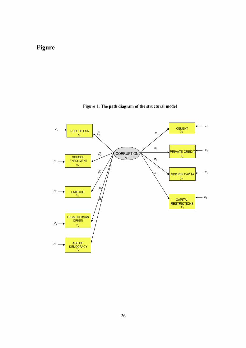
Figure 1 presents the hypothesized set of relationships that link the variable of inter-
est, corruption, to the indicators and causes.24 These constructs predict the measured
variable (corruption). The implication is that corruption is indicated by the country’s
cement consumption, private credit, GDP per capita and capital restrictions. The latent
variable of corruption is also predicated by a series of causal variables namely, the rule
of law, school enrolment, latitude, legal German origin and the age of democracy. The
model is then estimated to derive the values of the estimated parameters that link both
the causes and indicators to the latent variable.
Insert Figure 1 here.
Before reporting the results, one should draw attention to the issue of separating causes
from indicators. All models presented below employ the causal and indicator variables
24It is common practice to represent the measured variables (indicators) by squares and the latentvariables (factors) by circles. The hypothesized relationship between the variables are indicated by lines.Straight single-headed arrows represent one-way influences from the variable at the arrow base to thevariable to which the arrow points.
11
with their contemporaneous values. Clearly, this might give rise to endogeneity or reverse
causality issues. Some of the causal variables can equally plausibly be used as indicators,
and vice versa. As the MIMIC method is confirmatory in nature, it is inevitable we
decide upon a model that can be accepted or rejected a priori. In those cases where the
literature is indecisive about whether a variable is a cause or an indicator, we used the
variable either way to test for the robustness of our results. As it turns out, the results
are rather robust to exchanging causal and indicator variables. We also tried lagging the
quantitative causal variables by one period to deal with potential endogeneity. Again,
the results are not qualitatively affected by this.
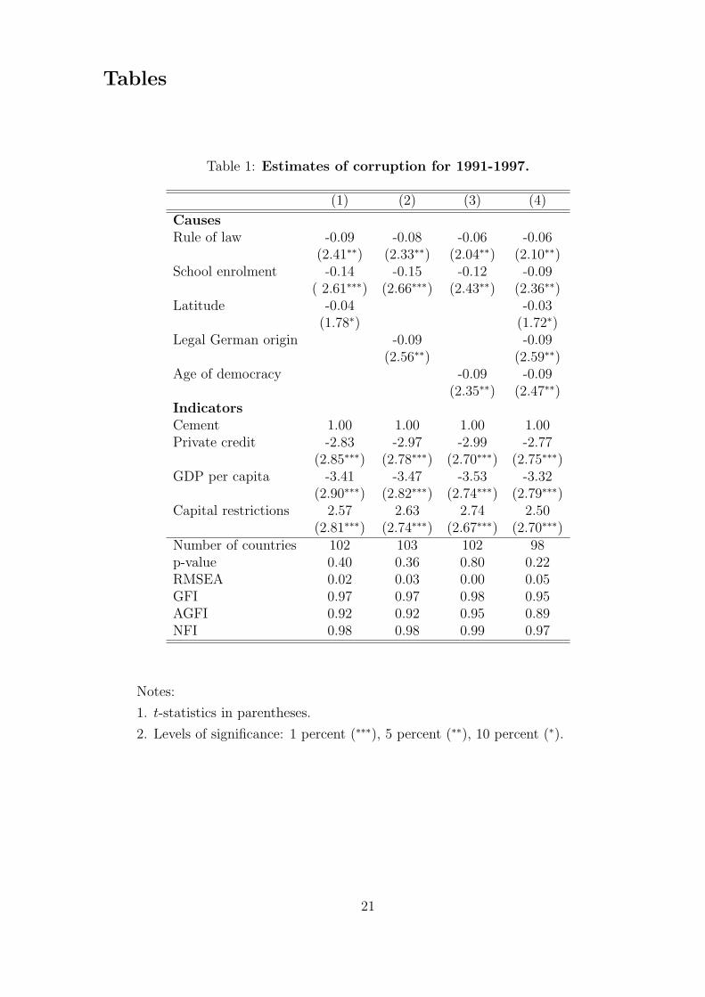
The results are presented in Table 1.
Insert Table 1 here.
Starting with the indicator variables, it can be seen that they are fairly consistent across
all model specifications. As pointed out in Section 2, one of the coefficients of the indica-
tors must be normalized for the estimated parameters to be identified. The choice of the
indicator variable on which to normalize the latent variable is to some extent arbitrary.
However, while the choice of indicator fixes the scale of the latent variable, the choice
does not affect the qualitative results (Stapleton, 1978). We choose cement consumption
for normalization as, theoretically, it is closely (and ideally directly) related to the un-
derlying concept of corruption. All indicator variables are statistically significant at the
1 percent level and have the anticipated sign, with cement consumption being positively
and financial development negatively related to corruption, respectively. Lower levels of
GDP per capita and more restrictions on the capital account are also associated with
higher corruption.
Turning to the causal variables, the results show that the rule of law has a negative effect
on corruption that is statistically significant at the 5 percent level across all specifications.
School enrolment, too, reduces corruption and so—recalling that school enrolment can
be interpreted as a proxy for the effectiveness of democracy in a given country—countries
with weak democratic institutions will be expected to have higher levels of corruption.
This coefficient is significant at the 1 percent level in the specifications reported in
columns 1 and 2, while it is significant at the 5 percent level in specifications 3 and 4.
Columns 1 and 4 include latitude (a variable with ambiguous economic interpretation).
At the 10 percent level of significance, latitude reduces corruption. Columns 2 and 4
also include a dummy for German legal origin, while the age of democracy is included
in columns 3 and 4. Both variables negatively affect corruption at the 5 percent level of
significance.25
25When including non-continuous variables, the estimator is no longer consistent, Bollen (1989). This,
12
In interpreting the relative effects of different explanatory variables, standardized coeffi-
cients are most useful.26 The standardized coefficient is the expected change in standard
deviation units of the latent variable when the other variables are held constant. Ac-
cording to the standardized coefficients of the full model (not reported in the Table) of
column 4, a one standard deviation increase in the rule of law leads to a reduction in
corruption by 0.20 standard deviations. A one standard deviation increase in the school
enrolment rate, latitude, and the age of democracy reduces corruption by 0.32, 0.12 and,
0.32 standard deviations, respectively.
Table 1 also reports goodness-of-fit statistics for the four model specifications. The chi-
square test of exact fit accepts all models at least at the five percent level of significance.27
The Root Mean Square Error of Approximation (RMSEA) accounts for the error of
approximation in the population and has recently been recognized as one of the most
informative criteria in covariance structure modelling (Steiger, 1990).28 The RMSEA
is smaller than 0.05 in the most recent period and still acceptable in the other three
specifications. Other indices providing evidence of an acceptable fit are the Goodness of
Fit Index (GFI), the Adjusted Goodness of Fit Index (AGFI) and the Normed Fit Index
(NFI). These indices range from zero to one, with values close to one indicating a better
fit.29 Based on these goodness-of-fit statistics, we conclude that the model fits the data
fairly well.
The next step is to derive the ranking for the countries in the sample in terms of their
expected levels of corruption. The method of proceeding from the estimated parameters
to the derivation of the index was outlined in Section 2. Specifically, the estimated
parameters together with the observations for the country-specific causes and indicators
however, does not seem to impose any problems here. The results are very similar when legal Germanorigin is excluded from estimation. Note that the index of restrictions is continuous due to averagingand standardizing.
26These standardized coefficients are defined as γsij = γij
√
σjj/σii, and βsij = βij
√
σjj/σii where thesubscript s denotes the standardized coefficient, i is the ‘dependent’ variable, j is the ‘independent’ and√
σjj ,√
σii are the model-predicted variances of the jth and ith variables, respectively.
27The chi-square statistic tests the specification of the model against the alternative that the co-variance matrix of the observed variables is unconstrained, where smaller values indicate a better fit.In other words, a small chi-square does not reject the null hypothesis that the model reproduces thecovariance matrix.
28Expressed differently, the RMSEA measures how well the model fits based on the difference betweenthe estimated and the actual covariance matrix (and degrees of freedom). Values of the RMSEA lessthan 0.05 indicate good fit, values as high as 0.08 represent reasonable fit, values from 0.08 to 0.10indicate mediocre fit, and those greater than 0.10 indicate poor fit (MacCallum et al. 1996).
29These indices are based on comparison with a null model predicting all covariances to be zero. TheNFI relates the chi-square of this null model to the chi-square of the actual model. It should be greaterthan 0.90. The GFI and the AGFI compare the loss function of the null model with the loss functionof the actual model, with AGFI adjusting for the complexity of the model.
13
are used to derive the latent scores and, in turn, the values for the index across the
countries in our sample.30 The results for the final model are reported in the first
column of Table 2, where the parentheses contain the index.
Insert Table 2 here.
The ranking, to a large extent, is not surprising, the developed countries being typically
reported as countries with lower corruption and developing countries with higher cor-
ruption. The world’s least corrupt country is Switzerland, followed by Japan, Norway,
Denmark, and Germany. With the exception of Japan, Singapore and the US, only West-
ern European countries are among the 15 least corrupt nations. At the bottom of the
scale, Guinea-Bissau, Nigeria, Syria, and the Central African Republic are found to be
the most corrupt. As can be seen, sub-Saharan African countries dominate the bottom
of the scale, with the exception of Syria, Ukraine, and Romania. Latin American and
Caribbean countries can be found at ranks between 31-71. To get a better understanding
of those regional differences, we also calculated average corruption indices according to
region. Corruption is by far lowest in Western Europe, with an average index of -0.36.
The ranking for the other regions is as follows: East Asia Pacific (-0.05), Middle East
and North Africa (0.16), Latin America and Caribbean (0.22), East Europe and Central
Asia (0.26), sub-Saharan Africa (0.29) and South Asia (0.29). Within Western Europe,
Greece is the most corrupt country followed by Portugal and Cyprus. The most corrupt
South Asian countries are Papua New Guinea, Philippines, and China. In the Middle
East and North Africa, Kuwait and Israel are the least, and Syria and Algeria the most,
corrupt countries. The least corrupt sub-Saharan Africa country is South Africa. In
what follows, we will explore the developments of these patterns over time.
4.2 Corruption 1976-1997
We now explore how corruption has changed over time since 1976. However, in doing
this, there are several drawbacks. First, the further back in time, the less data there is
available in terms of country coverage. For each sub-time period the model is estimated,
the sample size reduces considerably (for the periods 1986-1990, 1981-1985 and 1976-
1980 the sample reduces to 91, 77 and 65 countries, respectively). The second issue
relates to the countries we lose from the sample; typically those countries for which data
is absent will be the less developed ones where corruption may be expected to be high.31
30In the economics literature the normalized coefficients are sometimes multiplied by the corresponding(standardized) data to derive an estimate of the latent variable, (Frey and Weck-Hannemann (1984),and Loayza (1996)). The results reported are robust to this procedure. As noted earlier, we have optedto use the methodology of Joreskog (2000) which uses more structural information.
31According to the empirical analysis in Rosendorff and Vreeland (2006), democratic countries aremore willing to provide data than are other regimes. The exception is Switzerland where data on capital
14
In this case, it is likely that the estimated model will give less statistically significant
coefficients for the earlier periods.
To deal with these issues, the basic specification of the model included all causal vari-
ables discussed in Section 3. However, for different time periods, not all variables were
statistically significant. Therefore, to provide consistency in our specification across
sub-periods, we estimate a more parsimonious version of the model to the one that was
presented in Table 1.32 In choosing the most parsimonious version of the model, we
relied on the variables that would be statistically significant across all time periods and
the goodness-of-fit statistics. While all the indicator variables continued to perform well,
the number of statistically significant causes was reduced to two: the rule of law and the
school enrolment rate. The results for the estimation of the model for each sub-period
(including the 1991-97 period) are presented in columns 2-4 of Table 3.
Insert Table 3 here.
The estimated parameters for both the causal and indicator variables are fairly consistent
across each sub-period. The signs of the estimated parameters continue to hold (as in
the less parsimonious model for 1991-1997 presented in Table 2) while the parameter
values show little variation. Table 3 also reports goodness-of-fit statistics for our four
models. The chi-square test of exact fit accepts all models at least at the five percent
level of significance. The RMSEA is smaller than 0.05 in the most recent period and
still acceptable in the other three specifications. The other indices that provide evidence
of model fit (the GFI, the AGFI and the NFI), all indicate values relatively close to
1. Based on these goodness-of-fit statistics, we conclude that our model fits the sample
data fairly well when estimated for each sub-period.
The indices of corruption derived from those estimates are presented in the last four
columns of Table 2. There are two important results. First, levels of corruption seem to
be fairly consistent over time, as are the relative positions of countries.33 Second, there
are some obvious regional patterns. Overall, corruption in Western Europe decreased
since the mid-70s, whereas corruption increased in sub-Saharan Africa and Latin Amer-
ica/Caribbean. The pattern is more mixed in East Asia Pacific, where the huge decrease
in Japan’s level of corruption reduces the average level for the region, and the Middle
account restrictions are not available for earlier periods. This is because Switzerland only became amember of the IMF in 1992.
32Note that for the most recent period, the correlation between the full and the parsimonious modelis 0.998. The quality of our results is thus not reduced by estimating a more parsimonious model.
33In interpreting the ranking one has to keep in mind that in many cases a country moves up or downin the ranking because of missing data for other countries.
15
East/North Africa, with decreases in corruption in Israel and Malta and increases in
most other countries. The averages for the period 1976-1980 are -0.13 (West Europe),
-0.01 (East Asia Pacific), 0.05 (Middle East and North Africa), 0.7 (Latin America and
Caribbean), 0.1 (sub-Saharan Africa) and 0.1 (South Asia). It is also worth noting
that, of the 10 most corrupt countries reported in Table 2, all witnessed an increase in
corruption since the 1980s.
Comparing our results for the full model over the period 1991-97 with the 1997 corrup-
tion perception-based index produced by Transparency International, five of the coun-
tries shown to be among the worlds ten least corrupt countries according to our index,
also appear among the first ten countries in the Transparency International index. No
country of our ten least corrupt countries ranks below 21 in the Transparency Inter-
national’s listing. In spite of the high correlation, and the overall consistency, there
are some interesting discrepancies. As one example, Chile ranks 37 according to our
index, while Transparency International’s ranking shows it to be 23. Given the different
interpretations of the indices, Chile is thus perceived to be less corrupt as it actually is.
5 Further discussion
This study was predicated on the fact that perception-based indices of corruption have
recently been criticized as potentially biased and inaccurate measures of corruption across
countries, but are nevertheless widely used in the empirical literature on corruption due
to their availability, their extensive country coverage and lack of alternative measures. As
discussed in the introduction, those indices may not be reliable indicators of the degree of
corruption. Instead, they may just reflect a general perception of a country’s institutional
quality. In this paper, we have addressed these potential shortcomings while retaining
the advantages of cross-country coverage by employing a structural equation model that
addresses many of the concerns raised with respect to the survey-based indices.
Of course, one may argue that the estimated model does not capture the extent of cor-
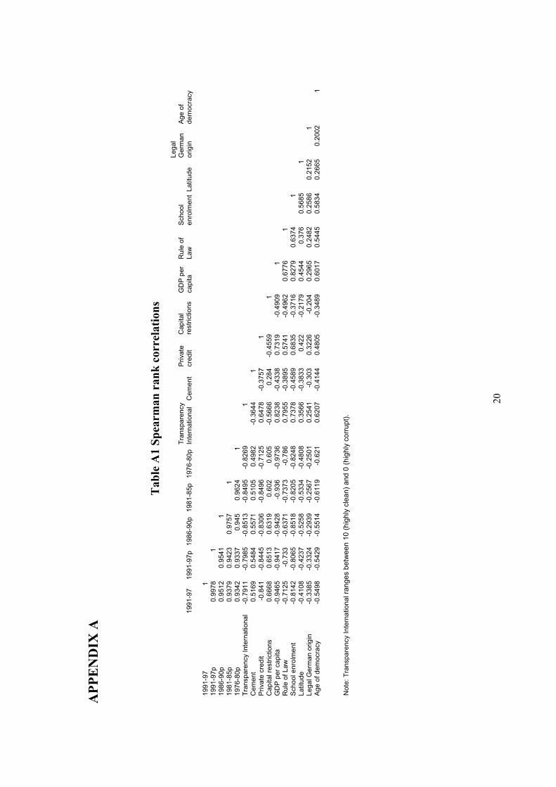
ruption. There are three ways to test for the validity of a structural model (Bollen, 1989).
Firstly, it is necessary to examine the fit of the model. Secondly, variables related to the
latent variable in the theoretical literature should have the expected impact. We have
dealt with these two validity tests above. Thirdly, the obtained latent variable should be
correlated with other measures of the same concept. We, therefore, calculated the cor-
relation of the resulting indices with the Corruption Perception Index of Transparency
International (which is highly correlated with other perception-based indices). As Ap-
pendix Table A1 shows, the resulting Spearman rank correlations for the respective time
16
periods range from 0.79 for the period 1991-97 to 0.85 in 1986-90.34 Overall, we can
be reasonably confident that our latent variable is picking up the ranking of corruption
across countries.
Arguably, reflecting the nature of the data, the index derived in this paper is likely
to be more appropriate to use in studies that evaluate the impact of corruption than
are perception-based indices. There are two important aspects to this. First, since the
index not only derives the rank but also the distance between countries in the corruption
index, this has the potential to give a more accurate (or less biased) estimate of how the
impact of corruption varies across countries and hence the dependent variable of interest.
Second, since the index is derived on country fundamentals that vary over time, the
ranking and the distance between countries can also vary over time. Moreover, the time
aspect has the potential to deal with any endogeneity issues between corruption and the
dependent variable since the lagged values of the corruption index may be exogenous to
current fundamentals.35
The use of the index may also provide a different assessment of the likely impact of
corruption to the one produced by perception-based indices.36 Indeed, a simple example
illustrates this point. Assessing the dependence of international cross-border acquisi-
tions (the main form of foreign direct investment) on the quality of institutions using
Transparency International’s perception-based index, for the US and OECD as host
countries and for the years 1997-2003, we found a substantial overestimation of the im-
pact of corruption on cross border mergers and acquisitions. More specifically, using the
perception-based corruption index of Transparency International, the absolute value of
the estimated standardized (beta-) coefficient is 0.16 which is substantially larger than
the estimated coefficient of 0.02 produced when using the corruption index reported in
this paper.37
Taken together, the corruption index based on the structural equation approach is likely
to be of direct consequence to different user groups. One such group is the policy-based
academic community which endeavor to evaluate the consequences of corruption. Since
34Table A1 also reports the correlation between the latent variables and the causal and indicatorvariables used. As can be seen, correlations between the latent variable and the indicators varies fromabout 0.5-0.95.
35This is a well accepted procedure in the shadow economy literature.
36This feature comes from the fact that the derived index provides a ranking between countries butalso a measure of distance. As such, it has the potential to more accurately estimate the impact ofcorruption on variables such as foreign direct investment.
37We make use of the index produced in Table 2 for the years 1991-1997 and the corruption perception-based index of Transparency International. The details are available upon request. The same patternemerges in the study of electoral competition and corruption, Herger (2005).
17
the measure derived here gives a measure of distance as well as ranking of corruption
across countries, it therefore has the potential to provide more reliable estimates of the
impact of corruption than perception-based indices which provide the ranking but not the
distance. As such, perception-based measures may provide biased estimates (as we note
above). For various international or private sector organizations and non-government
organizations who make decisions based on the institutional environment of a particular
country (e.g., the disbursement of aid or investment), the methodology for deriving an
index outlined here would also be potentially useful. The main advantage for this con-
stituent user is that it can monitor how corruption in a particular country varies over
time. Even if the ranking of the country in the corruption index stays the same, this
does not necessarily imply that corruption is not being controlled. Moreover, since the
perception-based indices have an in-built bias insofar as perceptions may change little
over time, countries may be denied aid and investment despite efforts to control corrup-
tion. Since the method outlined here is based on measurable causes and indicators that
vary over time, this allows a country’s measured performance in controlling corruption
to improve.
Clearly, the MIMIC method of structural equation modeling as applied here is only an
additional step in furthering our understanding about corruption. Generally, there is
considerable scope for using the structural equation methodology to explore broader
aspects of institutional governance and how it is linked to corruption. For example,
Glaeser et al. (2004) and Rodrik et al. (2004) have argued that conventionally-used
measures of institutional quality such as the rule of law are perception-based outcome
measures that do not necessarily pick up the quality of governance that they purport to
do. In this sense, applying the above methodology to measure institutional quality as
a latent variable with appropriate causes and indicators could be fruitful. In addition,
as already touched upon, the incidence of corruption may interact with measures of
institutional quality such that there is a potential endogeneity issue: corruption may be
high due to weak institutions, though the institutions may be weak because corruption
is so pervasive. The structural equation methodology has the potential to account for
this.38
6 Concluding remarks
Current policy focus on corruption around the world, as well as most empirical studies
of corruption, employ perception-based indices to gauge the ranking between the most
38For such a multiple latent approach see Dreher et al. (2006), who explore the link between theshadow economy and corruption in OECD countries.
18
and less corrupt countries. The recent literature has revealed several problems in the
interpretation of these indices. To this end, we employed a structural model of corruption
that simultaneously deals with the causes and indicators of corruption within a unified
framework.
There are clear advantages to using this framework to estimating corruption. First, the
model is explicitly causal in nature such that the ranking one retrieves across countries
is tied to the causal variables that were used to estimate the model. As such, the model
produces a cardinal index of corruption rather than one that is solely ordinal. Secondly,
dependent on data availability, the model can be estimated over different sub-periods to
assess how corruption has changed over time for each country.
The methodology applied in this paper holds much promise for future research in the
empirical analysis of corruption. For example, the impact of economic, political and
economic reform on corruption is a potentially fruitful avenue of research and one that
has received some attention for those who identify the role of institutions as a deter-
minant of economic development (Acemolgu et al. (2001) and Rodrik et al. (2002)).
Moreover, the methodology reported here can be extended to the case where some of
the exogenous variables are themselves inherently latent and interrelated (for example,
with institutional reform, the rule of law and the hidden economy) which interact with
the endogenous latent variable of corruption. For example, in measuring the size of the
hidden economy which has been a previous focus of researchers using MIMIC, the es-
timates are likely to be picking up aspects of corruption (and vice versa). Separating
these two aspects will provide a more accurate assessment of the relative importance of
each of them.
19
20
AP
PE
ND
IX A
Ta
ble
A1
Sp
earm
an
ra
nk
co
rrel
ati
on
s
199
1-9
71
99
1-9
7p
198
6-9
0p
198
1-8
5p
197
6-8
0p
Tra
nspa
ren
cy
Inte
rnation
al
Cem
en
t
Pri
vate
cre
dit
Ca
pital
restr
iction
sG
DP
pe
r
ca
pita
Ru
le o
f
La
w
Scho
ol
enro
lme
nt
Latitu
de
Leg
al
Ge
rma
n
ori
gin
Age
of
dem
ocra
cy
199
1-9
71
199
1-9
7p
0.9
97
81
198
6-9
0p
0.9
51
20.9
54
11
198
1-8
5p
0.9
37
90.9
42
30.9
75
71
197
6-8
0p
0.9
34
20.9
33
70.9
45
0.9
62
41
Tra
nsp
are
ncy I
nte
rnatio
nal
-0.7
91
1-0
.798
5-0
.851
3-0
.849
5-0
.826
91
Cem
en
t0.5
16
90.5
48
40.5
57
10.5
10
50.4
98
2-0
.364
41
Pri
vate
cre
dit
-0.8
41
-0.8
44
5-0
.830
6-0
.849
6-0
.712
50
.64
78
-0.3
75
71
Cap
ital re
str
ictions
0.6
66
80.6
51
30.6
31
90.6
02
0.6
05
-0.5
66
60.2
84
-0.4
55
91
GD
P p
er
ca
pita
-0.9
46
5-0
.941
7-0
.942
8-0
.93
6-0
.973
60
.82
38
-0.4
33
80.7
319
-0.4
90
91
Rule
of
La
w-0
.712
5-0
.73
3-0
.637
1-0
.737
3-0
.78
60
.79
55
-0.3
89
50.5
741
-0.4
96
20.6
77
61
Sch
oo
l e
nro
lmen
t-0
.814
2-0
.806
5-0
.851
8-0
.820
5-0
.824
80
.73
78
-0.4
58
90.6
835
-0.3
71
60.8
27
90.6
37
41
Latitu
de
-0.4
10
8-0
.423
7-0
.525
8-0
.533
4-0
.480
80
.35
66
-0.3
83
30.4
22
-0.2
17
90.4
54
40.3
76
0.5
68
51
Leg
al G
erm
an o
rig
in-0
.338
5-0
.332
4-0
.293
9-0
.256
7-0
.250
10
.25
41
-0.3
03
0.3
226
-0.2
04
0.2
96
50.2
48
20.2
58
60.2
15
21
Ag
e o
f d
em
ocra
cy
-0.5
49
8-0
.542
9-0
.551
4-0
.611
9-0
.62
10
.62
07
-0.4
14
40.4
805
-0.3
48
90.6
01
70.5
44
50.5
83
40.2
66
50.2
00
21
No
te:
Tra
nspa
rency In
tern
atio
na
l ra
ng
es b
etw
ee
n 1
0 (
hig
hly
cle
an)
and
0 (
hig
hly
co
rrup
t).
Tables
Table 1: Estimates of corruption for 1991-1997.
(1) (2) (3) (4)
Causes
Rule of law -0.09 -0.08 -0.06 -0.06(2.41∗∗) (2.33∗∗) (2.04∗∗) (2.10∗∗)
School enrolment -0.14 -0.15 -0.12 -0.09( 2.61∗∗∗) (2.66∗∗∗) (2.43∗∗) (2.36∗∗)
Latitude -0.04 -0.03(1.78∗) (1.72∗)
Legal German origin -0.09 -0.09(2.56∗∗) (2.59∗∗)
Age of democracy -0.09 -0.09(2.35∗∗) (2.47∗∗)
Indicators
Cement 1.00 1.00 1.00 1.00Private credit -2.83 -2.97 -2.99 -2.77
(2.85∗∗∗) (2.78∗∗∗) (2.70∗∗∗) (2.75∗∗∗)GDP per capita -3.41 -3.47 -3.53 -3.32
(2.90∗∗∗) (2.82∗∗∗) (2.74∗∗∗) (2.79∗∗∗)Capital restrictions 2.57 2.63 2.74 2.50
(2.81∗∗∗) (2.74∗∗∗) (2.67∗∗∗) (2.70∗∗∗)Number of countries 102 103 102 98p-value 0.40 0.36 0.80 0.22RMSEA 0.02 0.03 0.00 0.05GFI 0.97 0.97 0.98 0.95AGFI 0.92 0.92 0.95 0.89NFI 0.98 0.98 0.99 0.97
Notes:
1. t-statistics in parentheses.
2. Levels of significance: 1 percent (∗∗∗), 5 percent (∗∗), 10 percent (∗).
21
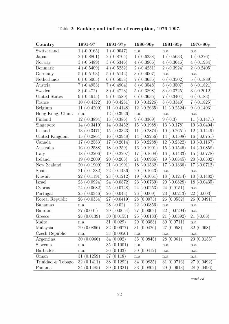
Table 2: Ranking and indices of corruption, 1976-1997.
Country 1991-97 1991-97P 1986-90P 1981-85P 1976-80P
Switzerland 1 (-0.9165) 1 (-0.9047) n.a. n.a. n.a.Japan 2 (-0.8801) 2 (-0.8705) 1 (-0.6238) 1 (-0.5633) 1 (-0.276)Norway 3 (-0.5489) 3 (-0.5346) 4 (-0.3966) 4 (-0.3646) 4 (-0.1984)Denmark 4 (-0.5409) 4 (-0.5232) 2 (-0.4231) 2 (-0.3924) 2 (-0.2405)Germany 5 (-0.5193) 5 (-0.5142) 3 (-0.4007) n.a. n.a.Netherlands 6 (-0.5005) 6 (-0.5058) 7 (-0.3635) 6 (-0.3502) 5 (-0.1889)Austria 7 (-0.4953) 7 (-0.4904) 8 (-0.3548) 5 (-0.3507) 8 (-0.1821)Sweden 8 (-0.472) 8 (-0.4723) 5 (-0.3898) 3 (-0.3725) 3 (-0.2012)United States 9 (-0.4615) 9 (-0.4589) 6 (-0.3635) 7 (-0.3404) 6 (-0.183)France 10 (-0.4322) 10 (-0.4281) 10 (-0.3226) 8 (-0.3349) 7 (-0.1825)Belgium 11 (-0.4209) 11 (-0.4148) 12 (-0.2665) 11 (-0.2524) 9 (-0.1493)Hong Kong, China n.a. 12 (-0.3926) n.a. n.a. n.a.Finland 12 (-0.3894) 13 (-0.386) 9 (-0.3369) 9 (-0.3) 11 (-0.1471)Singapore 14 (-0.3419) 14 (-0.3452) 15 (-0.1988) 13 (-0.178) 19 (-0.0404)Iceland 13 (-0.3471) 15 (-0.3323) 11 (-0.2874) 10 (-0.2651) 12 (-0.1449)United Kingdom 15 (-0.2864) 16 (-0.2948) 14 (-0.2256) 14 (-0.1598) 16 (-0.0751)Canada 17 (-0.2583) 17 (-0.2614) 13 (-0.2288) 12 (-0.2322) 13 (-0.1167)Australia 16 (-0.2588) 18 (-0.259) 16 (-0.1901) 15 (-0.1546) 14 (-0.0858)Italy 18 (-0.2206) 19 (-0.2207) 17 (-0.1608) 16 (-0.1433) 15 (-0.0778)Ireland 19 (-0.2009) 20 (-0.203) 21 (-0.0986) 19 (-0.0845) 20 (-0.0302)New Zealand 20 (-0.1909) 21 (-0.1991) 18 (-0.1532) 17 (-0.1336) 17 (-0.0712)Spain 21 (-0.1382) 22 (-0.1436) 20 (-0.1043) n.a. n.a.Kuwait 22 (-0.1191) 23 (-0.1212) 19 (-0.1061) 18 (-0.1214) 10 (-0.1482)Israel 23 (-0.0924) 24 (-0.0872) 23 (-0.0769) 20 (-0.0828) 18 (-0.0435)Cyprus 24 (-0.0682) 25 (-0.0748) 24 (-0.0253) 24 (0.0151) n.a.Portugal 25 (-0.0346) 26 (-0.043) 26 (-0.009) 23 (-0.0213) 22 (-0.003)Korea, Republic 26 (-0.0334) 27 (-0.0419) 28 (0.0073) 26 (0.0552) 26 (0.0491)Bahamas n.a. 28 (-0.02) 22 (-0.0856) n.a. n.a.Bahrain 27 (0.001) 29 (-0.0054) 27 (0.0002) 22 (-0.0294) n.a.Greece 28 (0.0139) 30 (0.0155) 25 (-0.0183) 21 (-0.0392) 21 (-0.03)Malta n.a. 31 (0.029) 29 (0.0383) 30 (0.0711) n.a.Malaysia 29 (0.0866) 32 (0.0677) 31 (0.0426) 27 (0.058) 32 (0.068)Czech Republic n.a. 33 (0.0856) n.a. n.a. n.a.Argentina 30 (0.0966) 34 (0.092) 35 (0.0845) 28 (0.061) 23 (0.0155)Slovenia n.a. 35 (0.1001) n.a. n.a. n.a.Barbados n.a. 36 (0.103) 30 (0.0412) n.a. n.a.Oman 31 (0.1259) 37 (0.118) n.a. n.a. n.a.Trinidad & Tobago 32 (0.1411) 38 (0.1292) 34 (0.0835) 31 (0.0716) 27 (0.0492)Panama 34 (0.1485) 39 (0.1321) 33 (0.0802) 29 (0.0613) 28 (0.0496)
cont.ed
22
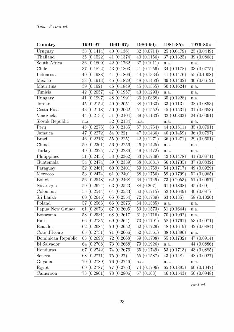
Table 2 cont.ed.
Country 1991-97 1991-97P 1986-90P 1981-85P 1976-80P
Uruguay 33 (0.1414) 40 (0.136) 32 (0.0714) 25 (0.0479) 25 (0.0449)Thailand 35 (0.1522) 41 (0.1374) 40 (0.1156) 37 (0.1325) 39 (0.0868)South Africa 36 (0.1809) 42 (0.1762) 37 (0.1011) n.a. n.a.Chile 37 (0.1822) 43 (0.1803) 41 (0.1256) 34 (0.1178) 33 (0.0775)Indonesia 40 (0.1988) 44 (0.1806) 44 (0.1334) 41 (0.1476) 55 (0.1008)Mexico 38 (0.1913) 45 (0.1829) 48 (0.1463) 39 (0.1402) 30 (0.0612)Mauritius 39 (0.192) 46 (0.1849) 45 (0.1355) 50 (0.1624) n.a.Tunisia 42 (0.2057) 47 (0.1957) 43 (0.1293) n.a. n.a.Hungary 41 (0.1997) 48 (0.1991) 36 (0.0868) 35 (0.1228) n.a.Jordan 45 (0.2152) 49 (0.2051) 38 (0.1133) 33 (0.113) 38 (0.0853)Costa Rica 43 (0.2118) 50 (0.2062) 51 (0.1552) 45 (0.1531) 31 (0.0653)Venezuela 44 (0.2135) 51 (0.2104) 39 (0.1133) 32 (0.0803) 24 (0.0361)Slovak Republic n.a. 52 (0.2184) n.a. n.a. n.a.Peru 48 (0.2275) 53 (0.2185) 67 (0.1754) 44 (0.1511) 35 (0.0791)Jamaica 47 (0.2272) 54 (0.22) 47 (0.1436) 40 (0.1459) 36 (0.0797)Brazil 46 (0.2216) 55 (0.225) 42 (0.1271) 36 (0.1271) 29 (0.0601)China 50 (0.2361) 56 (0.2256) 46 (0.1425) n.a. n.a.Turkey 49 (0.2325) 57 (0.2286) 49 (0.1472) n.a. n.a.Philippines 51 (0.2455) 58 (0.2362) 63 (0.1739) 42 (0.1478) 41 (0.0871)Guatemala 54 (0.2474) 59 (0.2389) 58 (0.1681) 56 (0.1735) 37 (0.0832)Paraguay 52 (0.2461) 60 (0.2401) 69 (0.1759) 54 (0.1717) 49 (0.0929)Morocco 53 (0.2474) 61 (0.2401) 68 (0.1756) 59 (0.1799) 52 (0.0965)Bolivia 56 (0.2548) 62 (0.2468) 64 (0.1749) 73 (0.2053) 51 (0.0957)Nicaragua 59 (0.2624) 63 (0.2523) 88 (0.207) 61 (0.1808) 45 (0.09)Colombia 55 (0.2544) 64 (0.2533) 60 (0.1715) 52 (0.1649) 40 (0.087)Sri Lanka 60 (0.2645) 65 (0.2554) 72 (0.1789) 63 (0.185) 58 (0.1026)Poland 57 (0.2565) 66 (0.2575) 54 (0.1585) n.a. n.a.Papua New Guinea 61 (0.2673) 67 (0.2605) 53 (0.1573) 51 (0.1644) n.a.Botswana 58 (0.2581) 68 (0.2617) 61 (0.1716) 70 (0.1992) n.a.Haiti 66 (0.2735) 69 (0.264) 73 (0.1791) 58 (0.1761) 53 (0.0971)Ecuador 62 (0.2684) 70 (0.2652) 62 (0.1729) 48 (0.1619) 42 (0.0884)Cote d’Ivoire 65 (0.2731) 71 (0.2666) 52 (0.1561) 38 (0.1396) n.a.Dominican Republic 63 (0.2698) 72 (0.2668) 59 (0.1708) 55 (0.1732) 47 (0.0914)El Salvador 64 (0.2708) 73 (0.2668) 79 (0.1926) n.a. 44 (0.0886)Honduras 67 (0.2742) 74 (0.2676) 65 (0.1749) 53 (0.1713) 43 (0.0885)Senegal 68 (0.2771) 75 (0.27) 55 (0.1587) 43 (0.148) 48 (0.0927)Guyana 70 (0.2789) 76 (0.2746) n.a. n.a. n.a.Egypt 69 (0.2787) 77 (0.2753) 74 (0.1796) 65 (0.1895) 60 (0.1047)Cameroon 73 (0.2861) 78 (0.2806) 57 (0.168) 46 (0.1543) 50 (0.0948)
cont.ed
23
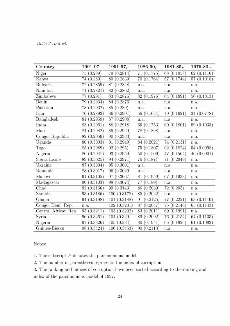
Table 2 cont.ed.
Country 1991-97 1991-97P 1986-90P 1981-85P 1976-80P
Niger 75 (0.289) 79 (0.2814) 71 (0.1775) 68 (0.1958) 62 (0.1116)Kenya 74 (0.289) 80 (0.2839) 70 (0.1764) 57 (0.1744) 57 (0.1018)Bulgaria 72 (0.2859) 81 (0.2848) n.a. n.a. n.a.Namibia 71 (0.2821) 82 (0.2862) n.a. n.a. n.a.Zimbabwe 77 (0.291) 83 (0.2876) 82 (0.1976) 64 (0.1891) 56 (0.1013)Benin 79 (0.2934) 84 (0.2876) n.a. n.a. n.a.Pakistan 78 (0.2932) 85 (0.289) n.a. n.a. n.a.Iran 76 (0.2892) 86 (0.2901) 56 (0.1634) 49 (0.1621) 34 (0.0778)Bangladesh 81 (0.2959) 87 (0.2908) n.a. n.a. n.a.India 83 (0.2961) 88 (0.2918) 66 (0.1753) 60 (0.1801) 59 (0.1033)Mali 84 (0.2982) 89 (0.2929) 78 (0.1898) n.a. n.a.Congo, Republic 82 (0.2959) 90 (0.2933) n.a. n.a. n.a.Uganda 86 (0.3003) 91 (0.2949) 84 (0.2021) 74 (0.2131) n.a.Togo 85 (0.2989) 92 (0.295) 75 (0.1807) 62 (0.1824) 54 (0.0998)Algeria 80 (0.2947) 93 (0.2959) 50 (0.1509) 47 (0.1564) 46 (0.0901)Sierra Leone 89 (0.3025) 94 (0.2971) 76 (0.187) 71 (0.2049) n.a.Ukraine 87 (0.3004) 95 (0.3001) n.a. n.a. n.a.Romania 88 (0.3017) 96 (0.3029) n.a. n.a. n.a.Malawi 91 (0.3105) 97 (0.3067) 81 (0.1959) 67 (0.1933) n.a.Madagascar 90 (0.3103) 98 (0.3074) 77 (0.189) n.a. n.a.Chad 92 (0.3166) 99 (0.3143) 86 (0.2039) 72 (0.205) n.a.Zambia 93 (0.3186) 100 (0.3178) 85 (0.2022) n.a. n.aGhana 94 (0.3198) 101 (0.3188) 91 (0.2125) 77 (0.2221) 63 (0.1119)Congo, Dem. Rep. n.a. 102 (0.3201) 87 (0.2047) 75 (0.2146) 65 (0.1143)Central African Rep. 95 (0.3211) 103 (0.3202) 83 (0.2011) 69 (0.1991) n.a.Syria 96 (0.3261) 104 (0.329) 89 (0.2092) 76 (0.2154) 64 (0.1135)Nigeria 97 (0.3326) 105 (0.334) 80 (0.1941) 66 (0.1926) 61 (0.1092)Guinea-Bissau 98 (0.3424) 106 (0.3453) 90 (0.2113) n.a. n.a.
Notes:
1. The subscript P denotes the parsimonious model.
2. The number in parentheses represents the index of corruption.
3. The ranking and indices of corruption have been sorted according to the ranking and
index of the parsimonious model of 1997.
24
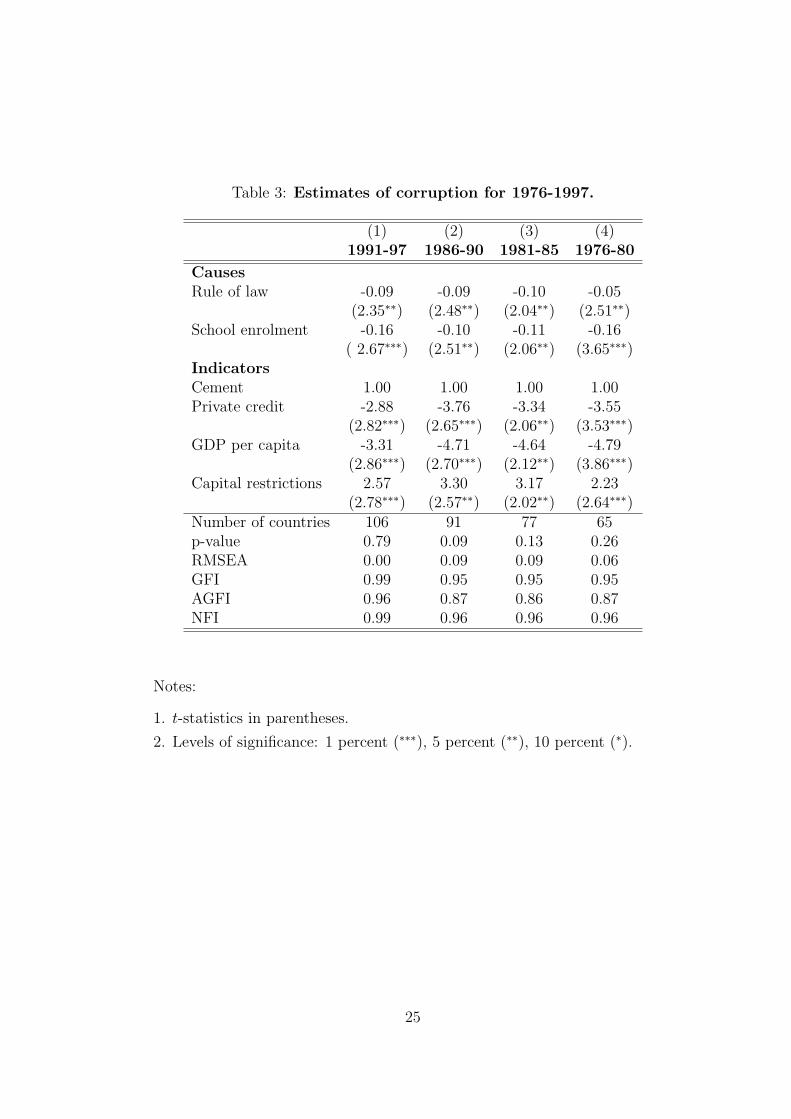
Table 3: Estimates of corruption for 1976-1997.
(1) (2) (3) (4)1991-97 1986-90 1981-85 1976-80
Causes
Rule of law -0.09 -0.09 -0.10 -0.05(2.35∗∗) (2.48∗∗) (2.04∗∗) (2.51∗∗)
School enrolment -0.16 -0.10 -0.11 -0.16( 2.67∗∗∗) (2.51∗∗) (2.06∗∗) (3.65∗∗∗)
Indicators
Cement 1.00 1.00 1.00 1.00Private credit -2.88 -3.76 -3.34 -3.55
(2.82∗∗∗) (2.65∗∗∗) (2.06∗∗) (3.53∗∗∗)GDP per capita -3.31 -4.71 -4.64 -4.79
(2.86∗∗∗) (2.70∗∗∗) (2.12∗∗) (3.86∗∗∗)Capital restrictions 2.57 3.30 3.17 2.23
(2.78∗∗∗) (2.57∗∗) (2.02∗∗) (2.64∗∗∗)Number of countries 106 91 77 65p-value 0.79 0.09 0.13 0.26RMSEA 0.00 0.09 0.09 0.06GFI 0.99 0.95 0.95 0.95AGFI 0.96 0.87 0.86 0.87NFI 0.99 0.96 0.96 0.96
Notes:
1. t-statistics in parentheses.
2. Levels of significance: 1 percent (∗∗∗), 5 percent (∗∗), 10 percent (∗).
25
26
Figure
CORRUPTION
CEMENT
PRIVATE CREDIT
GDP PER CAPITA
CAPITALRESTRICTIONS
AGE OF DEMOCRACY
SCHOOL
ENROLMENT
LATITUDE
LEGAL GERMANORIGIN
RULE OF LAW1
2
3
2z
1z
3z
4z
1y
2y
3y
4y
1! 1"
2"
3"#
1x
2x
3x
4x
2!
3!
4!
4"
4
Figure 1: The path diagram of the structural model
5!
5x
5
Appendix
The appendix provides the definitions of the variables and their sources.
Variables used in tables 1 and 3
Age of democracy: Number of years since 1900 a country has a democracy scorecontinuously greater than zero. Source: Marshall and Jaggers (2000).
Cement: Cement consumption measured in thousand tons adjusted by GDP andpopulation density. Source: Cembureau (1998, 1999).
GDP per capita: Domestic product divided by mid-year population. Source: WorldBank (2003).
Latitude: Distance in degrees from the equator, Easterly and Sewadeh (2001).
Legal origin: Dummies for British, French, German and Socialist legal origin. Source:Easterly and Sewadeh (2001).
Private credit: Private credit by deposit money banks and other financial institutionsas a share of GDP. Source: Beck et al. (1999).
Restrictions: Range 0 (no restrictions) to 4 (fully restricted). Consists of dummiesfor the existence of payments restrictions, multiple exchange rates, surrender re-quirements and restrictions on current transactions. Source: Dreher and Siemers(2003). This is a continuous variables, since it is averaged over seven (for the period1991-1997) and five years (for the periods 1976-1990).
Rule of law: 0-10 (0 = low; 10 = high) score for the quality of the legal system andproperty rights. Source: Gwartney et al. (2003).
School enrolment rate: Ratio of total enrolment to the population of the age groupthat officially corresponds to the level of education shown. Secondary educationcompletes the provision of basic education that began at the primary level. Source:World Bank (2003).
27
References
Acemoglu, D., J. A. Robinson and S. Johnson (2001) ‘The colonial origins of compar-ative development: an empirical investigation,’ American Economic Review 91:1369-1401.
Ades, A. and Di Tella, R. (1999) ‘Rents, competition and corruption,’ American Eco-nomic Review 89: 982-993.
Aidt, T. S. (2003) ‘Economic analysis of corruption: a survey,’ Economic Journal 113:632-652.
Alesina, A., A. Devleeschauewer, W. Easterly, S. Kurlat and R. Wacziarg (2003) ‘Frac-tionalization,’ Journal of Economic Growth 8: 155-194.
Andvig, J. C. (2005) ‘A house of straw, sticks or bricks’? Some notes on corruptionempirics, Paper presented to IV Global Forum on Fighting Corruption and Safe-guarding Integrity, Session Measuring Integrity, June 7, 2005.
Andvig, J-C., O-H. Fjeldstad, I. Amundsen, T. Sissener and T. Soreide (2000) Researchon corruption: A policy oriented survey. CMI and NUPI.
Banks, A. S. (1999) ‘Cross National Time-Series Data Archive,’ Banner Software, Inc.,Binghamton, NY.
Bardhan, P. (1997) ‘Corruption and development: A review of issues,’ Journal of Eco-nomic Literature 3: 1320-1346.
Becker, G. (1968) ‘Crime and punishment: An economic approach,’ Journal of PoliticalEconomy 76: 169-217.
Beck, T., A. Demirguc-Kunt and R. Levine (1999) ‘A new database on financial de-velopment and structure,’ Domestic Finance Working Paper 2146, World Bank,Washington, DC.
Beck, T., G. Clarke, A. Groff, P. Keefer and P. Walsh (2001) ‘New tools in comparativepolitical economy: the database of political institutions,’ World Bank EconomicReview 15(1): 165-176.
Bjørnskov, C. (2006) ‘The Multiple Facets of Social Capital, European Journal of Po-litical Economy, 22(1): 22-40.
Bollen, K. (1989) Structural equations with latent variables. Wiley.
Cembureau (1998) World Statistical Review No. 18, World Cement Market in Figures1913/1995: The European Cement Association, Brussels, Belgium.
Cembureau (1999) World Statistical Review No. 19 and 20: The European CementAssociation, Brussels, Belgium.
Claessens, S. and L. Laeven (2003) ‘Financial development, property rights and growth,’Journal of Finance LVIII: 2401-2436.
della Porta, D. and A. Vannucci (1997) ‘The “perverse effects” of political corruption,’Political Studies 45: 516-538.
Dreher, A. and M. Gassebner (2007) ‘Greasing the wheels of entrepreneurship? Theimpact of regulations and corruption on firm entry’, KOF Working Paper 166,ETH Zurich.
28
Dreher, A., C. Kotsogiannis and S. McCorriston (2006) ‘How do institutions affectcorruption and the shadow economy?,’ University of Exeter, mimeo.
Dreher, A. and L-H. R. Siemers (2005) ‘The intriguing nexus between corruption andcapital account restrictions,’ KOF Working Paper 113, ETH Zurich.
Easterly, W. and R. Levine (1997) ‘Africa’s growth tragedy: policies and ethnic divi-sions’ Quarterly Journal of Economics 112: 1203-1250.
Easterly, W. and M. Sewadeh (2001) ‘Global Development Network Growth Database,’http://www. worldbank.org/research/growth/GDNdata.htm.
Fisman, R. and R. Gatti (2002) ‘Decentralization and corruption: Evidence acrosscountries,’ Journal of Public Economics 83: 325-45.
Frey, B. S. and H. Weck-Hannemann (1984) ‘The hidden economy as an unobservedvariable,’ European Economic Review 26: 33-53.
Giles, D. E. (1999) ‘Measuring the hidden economy: implications for econometric mod-elling,’ The Economic Journal 109: F370-F380.
Gwartney, J., R. Lawson and N. Emerick (2003) ‘Economic freedom of the world: 2003annual report,’ Vancouver: The Fraser Institute, www. freetheworld.com.
Herger, N. (2005). ‘Electoral competition and corruption,’ mimeo, University of Exeter.
Herger, N., C. Kotsogiannis and S. McCorriston (2005) ‘International merger activityand the quality of institutions: An event count study,’ mimeo, University of Exeter.
Hillman, A. L. and M. Krausz (2004) ‘Development failure, corruption, and the financialsystem’, Paper presented at the European Public Choice Society Conference inBerlin, April 15-18, 2004.
IMF (2001) Government finance statistics, Washington, DC: International MonetaryFund.
Jain, A. K. (2001) ‘Corruption: a review,’ Journal of Economic Surveys 15: 71-121.
Johnston, M. and Y. Hao (1995) ‘China’s surge in corruption,’ Journal of Democracy6: 80-94.
Joreskog, K. G. and A. S. Goldberger (1975) ‘Estimation of a model with multipleindicators and multiple causes of a single latent variable,’ Journal of the AmericanStatistical Association 70: 631-639.
Joreskog, K. G. (2000) ‘Latent variable scores and their uses.’ Downloadable fromhttp://www.ssicentral.com/lisrel/column6.htm (accessed June 3, 2004).
Kaufmann, D., A. Kraay and P. Zoido-Lobaton (1999) ‘Governance matters,’ PolicyResearch Working Paper 2196, World Bank.
Kaufmann, D., A. Kraay and M. Mastruzzi (2003) ‘Governance matters III,’ WorldBank, Draft Paper.
Kaufmann, D. and S. J. Wei (1999) ‘Does “grease money” speed up the wheels ofcommerce,’ NBER Working Paper 7093, Cambridge, Mass.
Klitgaard, R. (1988). Controlling Corruption. Berkeley: University of California Press.
29
Knack, S., M. Kugler and N. Manning (2003) ‘Second-generation governance indicators,’International Review of Administrative Services 69: 345-364.
Kuklys, W. (2004) ‘Measuring Standard of Living in the UK - An Application of SensFunctioning Approach Using Structural Equation Models,’ mimeo, University ofCambridge and Max Planck Institute of Research Into Economic Systems.
Lambsdorff, J. Graf (1999) ‘Corruption in empirical research – a review,’ TransparencyInternational Working Paper, November 1999.
La Porta, R., F. Lopez-De-Silanes, A. Schleifer and R. Vishny (1999) ‘The quality ofgovernment,’ Journal of Law, Economics and Organization 15: 222-279.
Leff, N. H. (1964) ‘Economic development through bureaucratic corruption,’ AmericanBehavioural Scientist 8: 8-14.
Loayza, N. V. (1996) ‘The economics of the informal sector: a simple model and someempirical evidence from Latin America,’ Carnegie-Rochester Conference Series onPublic Policy 45: 129-162.
Lui, F. (1985) ‘An equilibrium queuing model of bribery,’ Journal of Political Economy93: 760-781.
MacCallum, R. C., M. W. Browne and H. M. Sugawara (1996) ‘Power analysis and de-termination of sample size for covariance structure modelling,’ Psychological Meth-ods 1: 130-149.
Marshall, M. G. and K. Jaggers (2000) ‘Polity IV project: political regime characteris-tics and transitions, 1800-2000’ http://www.cidcm.umd.edu/inscr/ polity/.
Mauro, P. (1995) ‘Corruption and growth,’ Quarterly Journal of Economics 110: 681-712.
Mauro, P. (1997) ‘Why worry about corruption?,’ Economic Issues 6. InternationalMonetary Fund, Washington.
Meon, P. and L. Weill (2006) ‘Is corruption and efficient grease?,’ mimeo.
Mocan, N. (2004) ‘What determines corruption? International Evidence from Microdata,’ NBER working paper 10460.
Morgan, T. (1964) ‘The theory of error in centrally-directed economic systems,’ Quar-terly Journal of Economics 78: 395-419.
Neeman, Z., D. Paserman and A. Simhon (2003) ‘Corruption and openness,’ CEPRDiscussion Paper No. 4057.
North, D. (1990) Institutions, institutional changes and economic performance. Cam-bridge University Press, Cambridge, UK.
Paldam, M. (2003) ‘The cross-country pattern of corruption: economics, culture andthe seesaw dynamics,’ European Journal of Political Economy 18: 215-240.
Persson, T., G. Tabellini, and F. Trebbi (2003) ‘Electoral Rules and Corruption,’ Jour-nal of the European Economic Association 4: 958 - 989.
Pickhardt, M. and Sarda Pons, J. (2006) ‘Size and Scope of the Underground Economyin Germany,’ forthcoming in Applied Economics.
30
Raiser. M, M. DiTommaso, and M. Weeks (2000) ‘The Measurement and Determina-tion of Institutional Change: Evidence from Transition Economics,’ DAE WorkingPaper, 29.
Razafindrakoto, M. and F. Rouboud (2006) Are international databases on corruptionreliable? A comparison of expert opinion surveys and household surveys in sub-Saharan Africa, Document de Travail DT/2006-17, DIAL, Paris.
Rodrik, D. A. Subramanian, and F. Trebbi (2002) ‘Institutions rule: the primacy ofinstitutions over geography and integration in economic development,’ CEPR Dis-cussion Paper 3643.
Rose-Ackerman, S. (1978) Corruption: A study in political economy. New York: Aca-demic Press.
Rose-Ackerman, S. (1999) Corruption and Government: Causes, Consequences andReform. Cambridge University Press, Cambridge, UK.
Rosendorff, P. and J. Vreeland (2006) ‘Democracy and Data Dissemination: The Effectof Political Regime on Transparency’, manuscript.
Schneider, F. (2005) ‘Shadow economies around the world: what do we really know?,’European Journal of Political Economy 21: 598-642.
Schneider, F. and D. H. Enste (2000) ‘Shadow economies: size, causes and conse-quences,’ Journal of Economic Literature XXXVIII, 77-114.
Schneider, F. and D. H. Enste (2002) The shadow economy: An international survey.Cambridge University Press.
Seldadyo, H. and J. de Haan (2005) ‘The determinants of corruption: A reinvestigation,’Paper presented at the EPCS 2005 meeting in Durham.
Søreide, T. (2005) ‘Is it right to rank? Limitations, implications and potential improve-ments of corruption indices,’ Paper presented to IV Global Forum on FightingCorruption and Safeguarding Integrity, Session Measuring Integrity, June 7, 2005.
Stapleton, D. C. (1978) ‘Analyzing political participation data with as MIMIC model,’Sociological Methodology 15: 52-74.
Steiger, J. H. (1990) ‘Structural model evaluation and modification: An interval esti-mation approach,’ Multivariate Behavioral Research 25: 173-180.
Svensson, J. (2005) ‘Eight questions about corruption,’ Journal of Economic Perspec-tives, 19: 19-42.
Tanzi, V. (1998) ‘Corruption around the world-causes, consequences, scope and cures,’International Monetary Fund Staff Papers 45: 559-594.
Treisman, D. (2000) ‘The causes of corruption: a cross-national study,’ Journal ofPublic Economics 76: 399-457.
Van Rijckeghem, C. and B. Weder (2001) ‘Bureaucratic corruption and the rate oftemptation; do wages in the civil service affect corruption and by how much?,’Journal of Development Economics 65: 307-331.
Varese, F. (1997) ‘The transition to the market and corruption in post-Socialist Russia,’Political Studies 45: 579-596.
31
Weber Abramo, C. (2005) ‘How far perceptions go,’ Transparency Brazil Working Pa-per.
Weck, H. (1983) Schattenwirtschaft: Eine Moglichkeit zur Einschrankung der offentlichenVerwaltung? Eine okonomische Analyse. Finanzwissenschaftliche Schriften 22,Lang, Bern/Frankfurt.
Wei, S-J. and Y. Wu (2001) ‘Negative alchemy? Corruption, composition of capitalflows and currency crises,’ Harvard University, mimeo.
World Bank (2001) http://www.worldbank.org/publicsector/anticorrupt/index.ctm.
World Bank (2003) ‘World Development Indicators’ CD-ROM, Washington, DC.
World Bank (2004) http://www.worldbank.org/WBSITE/EXTERNAL/NEWS. Ac-cessed 21 April 2004.
32
THIS APPENDIX IS FOR THE ATTENTION OF THE REFEREESONLY AND NOT FOR PUBLICATION
This appendix lists the causal and indicator variables that were tried, but without suc-cess: the criterion for the selection of variables being that data are available for a sufficientnumber of countries and periods.
Causal variables
Degree of democracy: 0-10 (0 = low; 10 = high) democracy score. Measures thegeneral openness of political institutions. Source: Marshall and Jaggers (2000).
Degree of political stability: Index constructed with principal components analysis.The weights obtained for the components are 0.08 (assassinations), 0.1 (strikes),0.25 (guerrilla warfare), 0.15 (crises), 0.16 (riots) and 0.27 (revolutions). Source:Banks (1999).
Dominant religion: Dummies equalling one if majority of population is catholic,protestant or muslim. Source: Alesina et al. (2003).
English as dominant language: Dummy that equals one if English is dominantlanguage. Source: Alesina et al. (2003).
Ethnic fractionalization: Definition as above. Source: Alesina et al. (2003).
Extent of decentralization: Sub-national revenues as a percent of total revenues and,respectively, sub-national expenditures as a percent of total expenditures. Source:IMF (2001).
Federal political system: Dummies for the existence of autonomous regions andlocally elected state/province governments. Source: Beck et al. (2001).
Freedom of the press: various years. Source: Freedom House, Press Freedom Survey(http://www.freedomhouse.org/research/ pressurvey.htm).
Former colony of Britain: Dummy indicating whether country was a British colony.Source: Acemoglu et al. (2001).
Fractionalization of government, opposition, and overall: The probability thattwo deputies picked at random from among the government, the opposition or,respectively, the whole legislature will be of different parties. Source: Beck et al.(2001).
Government consumption: General government final consumption expenditure (inpercent of GDP). Source: World Bank (2003).
Government revenue: General government final consumption expenditure in percentof GDP. Source: World Bank (2003).
Legal origin: Dummies for British, French, German and Socialist legal origin. Source:Easterly and Sewadeh (2001).
Linguistic fractionalization: Definition as above. Source: Alesina et al. (2003).
Natural resource exports: Fuel exports (percent of merchandize exports), ores andmetals exports (percent of merchandize exports). Source: World Bank (2003).
Presidential political system: Dummy that equals one if the political system ispresidential. Source: Beck et al. (2001).
33
Religious fractionalization: Fractionalization of group i in country j is determinedby 1 −
∑n
i=1s2
ij with sij being the share of group i in country j. Source: Alesinaet al. (2003).
Settler mortality: Log of estimated settler mortality. Acemoglu et al. (2001).
Trade as a percentage of GDP: The sum of exports and imports of goods andservices measured as a share of GDP. Source: World Bank (2003).
Years in office: The number of years the incumbent government has already been inoffice. Source: Beck et al. (2001).
Other indicator variables
Growth of GDP: Annual percentage growth rate of GDP based on constant localcurrency. Source: World Bank (2003).
Growth of GDP per capita: Annual percentage growth rate of GDP per capitabased on constant local currency. Source: World Bank (2003).
Public Investment: Gross domestic investment in percent of GDP. Source: WorldBank (2003).
Trade: Sum of exports and imports of goods and services measured as a share of grossdomestic product in percent of GDP. Source: World Bank (2003).
34