Embed Size (px)
Citation preview
LICOS Centre for Transition Economics
LICOS Discussion Papers
Discussion Paper 175/2006
“Skating on Thin Ice : Rule Changes and Team Strategies in the NHL”
Anurag N. Banerjee Johan F.M. Swinnen
Alfons Weersink
Katholieke Universiteit Leuven
LICOS Centre for Transition Economics Huis De Dorlodot Deberiotstraat 34 B-3000 Leuven
BELGIUM TEL:+32-(0)16 32 65 98 FAX:+32-(0)16 32 65 99
http://www.econ.kuleuven.be/licos
Skating on Thin Ice :
Rule Changes and Team Strategies in the NHL. 1
Anurag N. BANERJEE
Department of Economics and Finance, University of Durham, Durham, UK
Johan F.M. SWINNEN,
Department of Economics, K. U. Leuven, Leuven, Belgium
Alfons WEERSINK,
Dept of Agricultural Economics and Business, University of Guelph,
Guelph, Ontario, CANADA
June, 2006
1The authors are grateful to the seminar participants at National University Singapore and
two referees for their constructive comments. The opinions expressed in this paper are those of
the authors and do not represent those of the institutions they are associated with.
Abstract
In an e¤ort to stimulate a more exciting and entertaining style of play, the National
Hockey Association (NHL) changed the rewards associated with the results of overtime
games. Under the new rules, teams tied at the end of regulation both receive a single
point regardless of the outcome in overtime. A team scoring in the sudden-death 5-minute
overtime period would earn an additional point. Prior to the rule change in the 1999-2000
season, the team losing in overtime would receive no points while the winning team earned
2 points. This paper presents a theoretical model to explain the e¤ect of the rule change
on the strategy of play during both the overtime period and the regulation time game.
The results suggest that under the new overtime format equally powerful teams will play
more o¤ensively in overtime resulting in more games decided by a sudden-death goal. The
results also suggest that while increasing the likelihood of attacking in overtime, the rule
change would have a perverse e¤ect on the style of play during regulation by causing them
to play conservatively for the tie. Empirical data con�rm the theoretical results. The
paper also shows that increasing the rewards to a win in regulation time would prevent
teams from playing defensively during regular time.
JEL Classi�cation C72, L83
Keywords: Ice Hockey, Game Theory, NHL Overtime Rule.
1 Introduction
Economic studies on the in�uence of rules, institutions and incentive structures on behav-
ior are complicated by the fact that incentives and observations on behavior are a¤ected
by a variety of factors outside the relationship of interest. For this reason, environments
which eliminate some of these outside in�uences are of particular interest. Some recent
studies have used observed data from sporting competitions to assess the e¤ects of incen-
tives. Rule changes in sports provide a unique natural experiment to test the consequences
of theoretical payo¤ structures. For example, the performance of individual competitors
has been shown to increase directly with the level of rewards in the sports ranging from
bowling (Ehrenberg and Bognanno 1990) to auto racing (Maloney and Terkun, 2002). In
terms of team sports, Banerjee and Swinnen (2003) use a game theoretic model along
with empirical evidence to show that the introduction of a sudden death rule in soccer
has not changed the style of play despite FIFA�s reasoning of introducing a "golden goal"
for more aggressive play during extra time. Similar rule changes were recently introduced
in professional ice hockey.
Despite the inherent attraction associated with the speed and action of ice hockey,
the popularity in North America of the game�s premier professional league, the National
Hockey League (NHL), lags behind that of the other three major professional sports
leagues, the National Football League (NFL), Major League Baseball (MLB), and the
National Basketball Association (NBA). The NHL has attempted to increase the general
appeal of the game by introducing several rule changes ranging from tougher �ghting
penalties to increasing the size of the area behind the nets. One of the most signi�cant
changes was the introduction in the 1983-84 season of a 5 minute, sudden-death overtime
period to settle any regular season games that had ended in a tie. A team scoring in
overtime would receive 2 points for the win while the losing team got 0 points for the loss.
Each team received a single point if the game remained tied at the end of overtime. In
an e¤ort to combat the perceived conservative play in overtime, the NHL implemented a
new point structure in the 1999-2000 season. Teams tied at the end of regulation would
both receive a single point regardless of the outcome in overtime. A team scoring in
the sudden-death overtime would earn an additional point. While the intent of the rule
change was to increase the excitement of the game through a more attacking style of play
in the overtime, the change in the reward system could have a perverse and opposite e¤ect
on the style of play.
The purpose of this paper is to determine the e¤ect of changes in overtime rules on
the play by NHL teams during regulation time and in overtime. The paper begins with a
game theoretic model that determines optimal team strategies under alternative overtime
point systems. The theoretical results suggest that rule changes should result in more
overtime games being decided within the extra-time period but that more games will end
1
up tied after the normal 60 minute regulation time. Empirical results are then presented
con�rming the hypotheses in section 3. Implications of other rule changes are assessed in
the conclusions.
2 Payo¤ Structures
The time points are de�ned such that teams can score a maximum of one goal during each
time point.1 We begin by breaking the game involving teams A and B into an arbitrary
set of T discrete time points N = f1; : : : ; t; : : : ; Tg. For example, t may represent a
minute of play in a hockey game.
Consider the game from the point of view of team A. At every t; the state of the game
for team A is described by the random state vector Xt; where
Xt =
8><>:1; if team A scores a goal, at time t,
0; if neither team scores a goal, at time t,
�1; if team B scores a goal, at time t.
The probabilities of this random variable are given by
Pr (Xt = 1) = p; Pr (Xt = �1) = q and Pr (Xt = 0) = r = 1� p� q:
The probability of teamA scoring a goal is the same as the probability of team B conceding
a goal. This implies that the state vector of team B is �Xt: At every instant t there is a
zero sum game between A and B implying that both cannot score during the same time
point. The probabilities p and q are functions of the actions of the teams.
Each team decides before the start of each time point on their playing strategy. We
assume the strategies are de�ned in terms of two actions, defensive play, denoted by L,
and o¤ensive play, denoted by H. We de�ne the actions sets of the two teams at a given
moment t as SAt and SBt ; where S
it = fH;Lg; i = A;B:
The probability functions p and q are de�ned as
p : SAt � SBt ! [0; 1] and q : SAt � SBt ! [0; 1]:
We assume that the probability of scoring is higher with o¤ensive play; formally:
p (H; :) > p (L; :) and q (:; H) > q (:; L) (2.1)
Further throughout the paper, we shall assume that the teams involved are equally likely to
score under identical situations and similar styles of play. This is a reasonable assumption
given the fact that a game is more likely to go to extra times if the teams are of similar
qualities (a similar assumption is made by Palomino et al. (1999) and Banerjee and
Swinnen (2004)). Formally:
1In hockey, there are three stop-time periods of 20 minutes in a regulation game and a 5 minute
sudden-death overtime period if the game is tied after 60 minutes of regulation play.
2
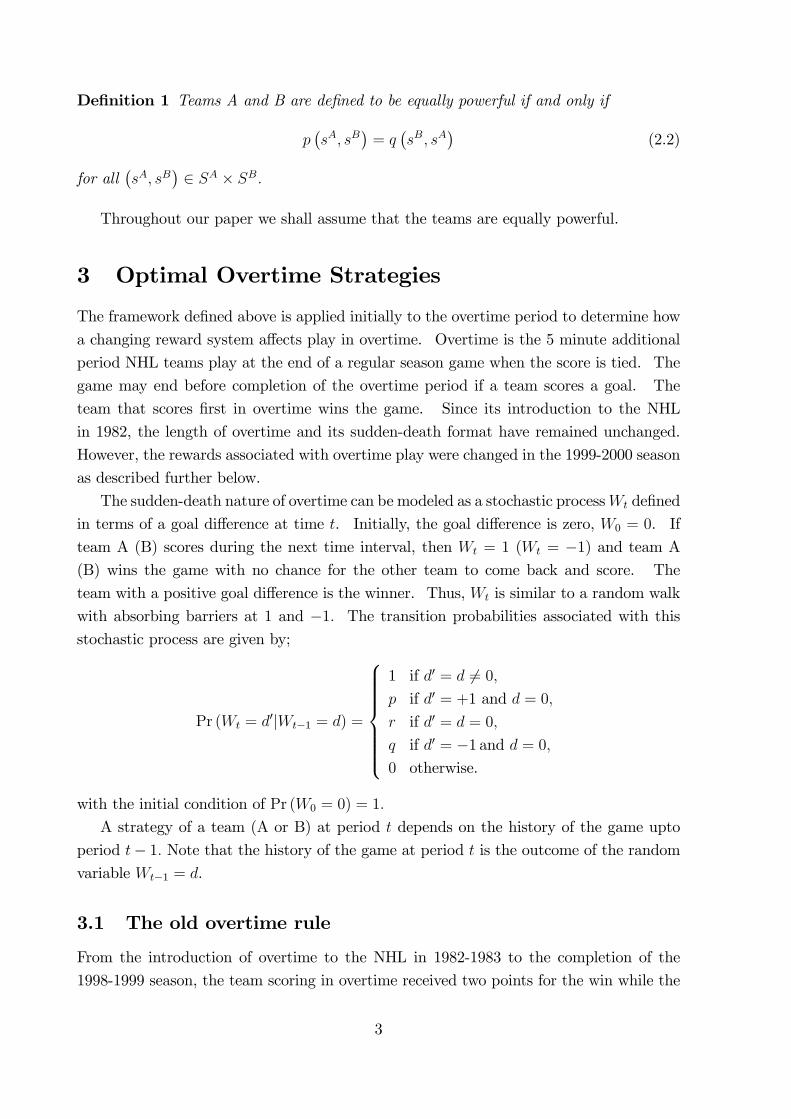
De�nition 1 Teams A and B are de�ned to be equally powerful if and only if
p�sA; sB
�= q
�sB; sA
�(2.2)
for all�sA; sB
�2 SA � SB:
Throughout our paper we shall assume that the teams are equally powerful.
3 Optimal Overtime Strategies
The framework de�ned above is applied initially to the overtime period to determine how
a changing reward system a¤ects play in overtime. Overtime is the 5 minute additional
period NHL teams play at the end of a regular season game when the score is tied. The
game may end before completion of the overtime period if a team scores a goal. The
team that scores �rst in overtime wins the game. Since its introduction to the NHL
in 1982, the length of overtime and its sudden-death format have remained unchanged.
However, the rewards associated with overtime play were changed in the 1999-2000 season
as described further below.
The sudden-death nature of overtime can be modeled as a stochastic processWt de�ned
in terms of a goal di¤erence at time t. Initially, the goal di¤erence is zero, W0 = 0. If
team A (B) scores during the next time interval, then Wt = 1 (Wt = �1) and team A
(B) wins the game with no chance for the other team to come back and score. The
team with a positive goal di¤erence is the winner. Thus, Wt is similar to a random walk
with absorbing barriers at 1 and �1: The transition probabilities associated with thisstochastic process are given by;
Pr (Wt = d0jWt�1 = d) =
8>>>>>><>>>>>>:
1 if d0 = d 6= 0;p if d0 = +1 and d = 0;
r if d0 = d = 0;
q if d0 = �1 and d = 0;0 otherwise.
with the initial condition of Pr (W0 = 0) = 1:
A strategy of a team (A or B) at period t depends on the history of the game upto
period t� 1: Note that the history of the game at period t is the outcome of the randomvariable Wt�1 = d.
3.1 The old overtime rule
From the introduction of overtime to the NHL in 1982-1983 to the completion of the
1998-1999 season, the team scoring in overtime received two points for the win while the
3
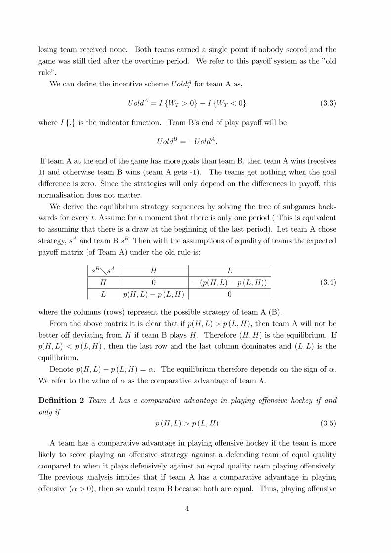
losing team received none. Both teams earned a single point if nobody scored and the
game was still tied after the overtime period. We refer to this payo¤ system as the �old
rule�.
We can de�ne the incentive scheme UoldAT for team A as,
UoldA = I fWT > 0g � I fWT < 0g (3.3)
where I f:g is the indicator function. Team B�s end of play payo¤ will be
UoldB = �UoldA:
If team A at the end of the game has more goals than team B, then team A wins (receives
1) and otherwise team B wins (team A gets -1). The teams get nothing when the goal
di¤erence is zero. Since the strategies will only depend on the di¤erences in payo¤, this
normalisation does not matter.
We derive the equilibrium strategy sequences by solving the tree of subgames back-
wards for every t: Assume for a moment that there is only one period ( This is equivalent
to assuming that there is a draw at the beginning of the last period). Let team A chose
strategy, sA and team B sB: Then with the assumptions of equality of teams the expected
payo¤ matrix (of Team A) under the old rule is:
sB�sA H L
H 0 � (p(H;L)� p (L;H))L p(H;L)� p (L;H) 0
(3.4)
where the columns (rows) represent the possible strategy of team A (B):
From the above matrix it is clear that if p(H;L) > p (L;H), then team A will not be
better o¤ deviating from H if team B plays H: Therefore (H;H) is the equilibrium. If
p(H;L) < p (L;H) ; then the last row and the last column dominates and (L;L) is the
equilibrium.
Denote p(H;L)� p (L;H) = �: The equilibrium therefore depends on the sign of �:
We refer to the value of � as the comparative advantage of team A.
De�nition 2 Team A has a comparative advantage in playing o¤ensive hockey if and
only if
p (H;L) > p (L;H) (3.5)
A team has a comparative advantage in playing o¤ensive hockey if the team is more
likely to score playing an o¤ensive strategy against a defending team of equal quality
compared to when it plays defensively against an equal quality team playing o¤ensively.
The previous analysis implies that if team A has a comparative advantage in playing
o¤ensive (� > 0), then so would team B because both are equal. Thus, playing o¤ensive
4
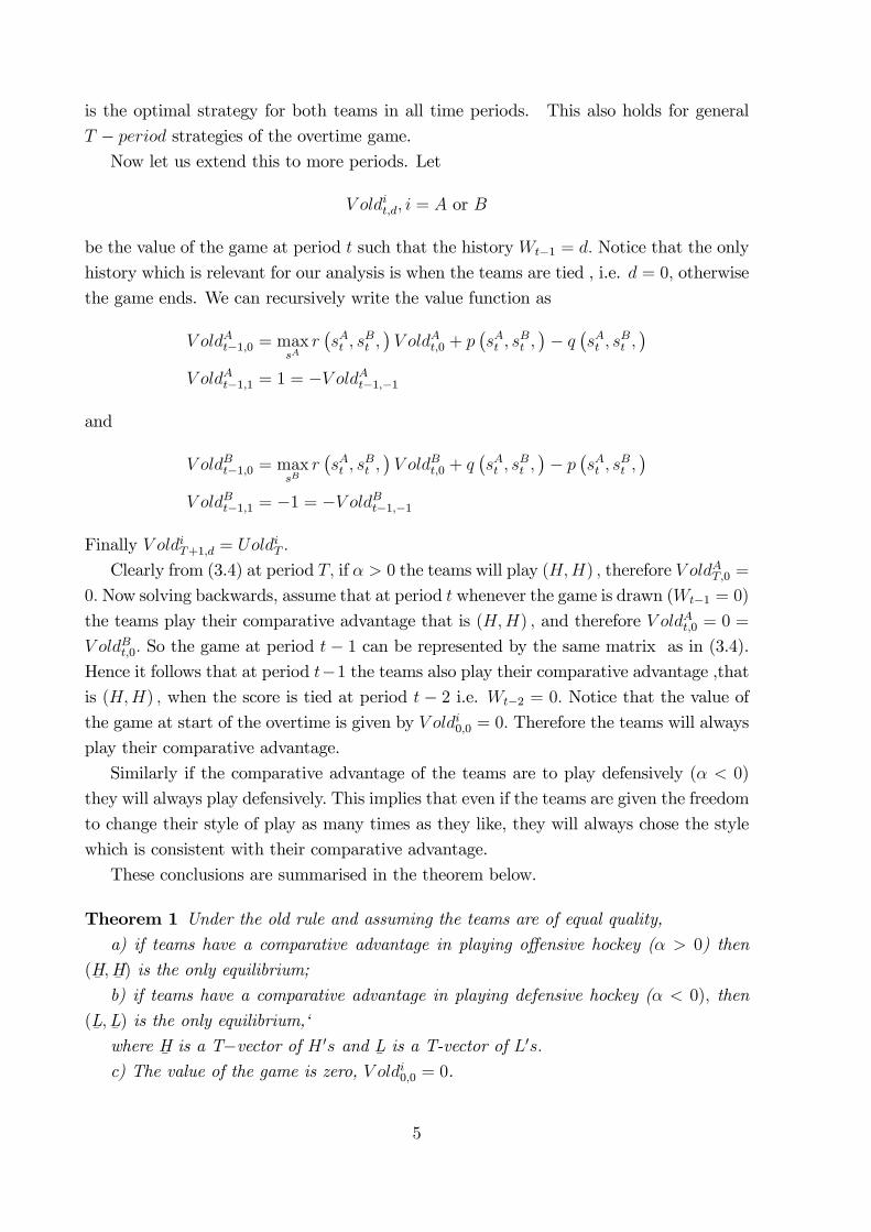
is the optimal strategy for both teams in all time periods. This also holds for general
T � period strategies of the overtime game.Now let us extend this to more periods. Let
V oldit;d; i = A or B
be the value of the game at period t such that the history Wt�1 = d: Notice that the only
history which is relevant for our analysis is when the teams are tied , i.e. d = 0; otherwise
the game ends. We can recursively write the value function as
V oldAt�1;0 = maxsAr�sAt ; s
Bt ;�V oldAt;0 + p
�sAt ; s
Bt ;�� q
�sAt ; s
Bt ;�
V oldAt�1;1 = 1 = �V oldAt�1;�1
and
V oldBt�1;0 = maxsB
r�sAt ; s
Bt ;�V oldBt;0 + q
�sAt ; s
Bt ;�� p
�sAt ; s
Bt ;�
V oldBt�1;1 = �1 = �V oldBt�1;�1
Finally V oldiT+1;d = UoldiT :
Clearly from (3.4) at period T; if � > 0 the teams will play (H;H) ; therefore V oldAT;0 =
0: Now solving backwards, assume that at period t whenever the game is drawn (Wt�1 = 0)
the teams play their comparative advantage that is (H;H) ; and therefore V oldAt;0 = 0 =
V oldBt;0: So the game at period t� 1 can be represented by the same matrix as in (3.4).
Hence it follows that at period t�1 the teams also play their comparative advantage ,thatis (H;H) ; when the score is tied at period t � 2 i.e. Wt�2 = 0: Notice that the value of
the game at start of the overtime is given by V oldi0;0 = 0: Therefore the teams will always
play their comparative advantage.
Similarly if the comparative advantage of the teams are to play defensively (� < 0)
they will always play defensively. This implies that even if the teams are given the freedom
to change their style of play as many times as they like, they will always chose the style
which is consistent with their comparative advantage.
These conclusions are summarised in the theorem below.
Theorem 1 Under the old rule and assuming the teams are of equal quality,a) if teams have a comparative advantage in playing o¤ensive hockey (� > 0) then
(H¯;H¯) is the only equilibrium;
b) if teams have a comparative advantage in playing defensive hockey (� < 0); then
(L¯;L¯) is the only equilibrium,�
where H¯is a T�vector of H 0s and L
¯is a T-vector of L0s:
c) The value of the game is zero, V oldi0;0 = 0.
5
3.2 The new overtime rule
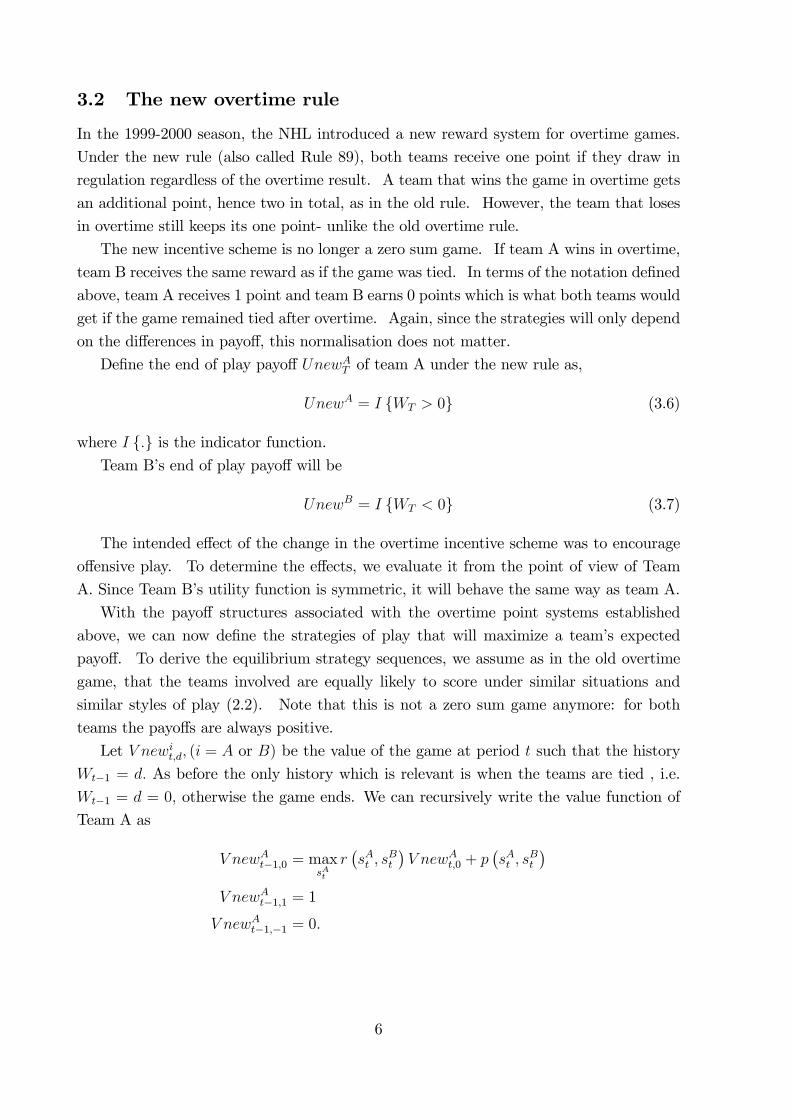
In the 1999-2000 season, the NHL introduced a new reward system for overtime games.
Under the new rule (also called Rule 89), both teams receive one point if they draw in
regulation regardless of the overtime result. A team that wins the game in overtime gets
an additional point, hence two in total, as in the old rule. However, the team that loses
in overtime still keeps its one point- unlike the old overtime rule.
The new incentive scheme is no longer a zero sum game. If team A wins in overtime,
team B receives the same reward as if the game was tied. In terms of the notation de�ned
above, team A receives 1 point and team B earns 0 points which is what both teams would
get if the game remained tied after overtime. Again, since the strategies will only depend
on the di¤erences in payo¤, this normalisation does not matter.
De�ne the end of play payo¤ UnewAT of team A under the new rule as,
UnewA = I fWT > 0g (3.6)
where I f:g is the indicator function.Team B�s end of play payo¤ will be
UnewB = I fWT < 0g (3.7)
The intended e¤ect of the change in the overtime incentive scheme was to encourage
o¤ensive play. To determine the e¤ects, we evaluate it from the point of view of Team
A. Since Team B�s utility function is symmetric, it will behave the same way as team A.
With the payo¤ structures associated with the overtime point systems established
above, we can now de�ne the strategies of play that will maximize a team�s expected
payo¤. To derive the equilibrium strategy sequences, we assume as in the old overtime
game, that the teams involved are equally likely to score under similar situations and
similar styles of play (2.2). Note that this is not a zero sum game anymore: for both
teams the payo¤s are always positive.
Let V newit;d; (i = A or B) be the value of the game at period t such that the history
Wt�1 = d: As before the only history which is relevant is when the teams are tied , i.e.
Wt�1 = d = 0; otherwise the game ends. We can recursively write the value function of
Team A as
V newAt�1;0 = maxsAt
r�sAt ; s
Bt
�V newAt;0 + p
�sAt ; s
Bt
�V newAt�1;1 = 1
V newAt�1;�1 = 0:
6
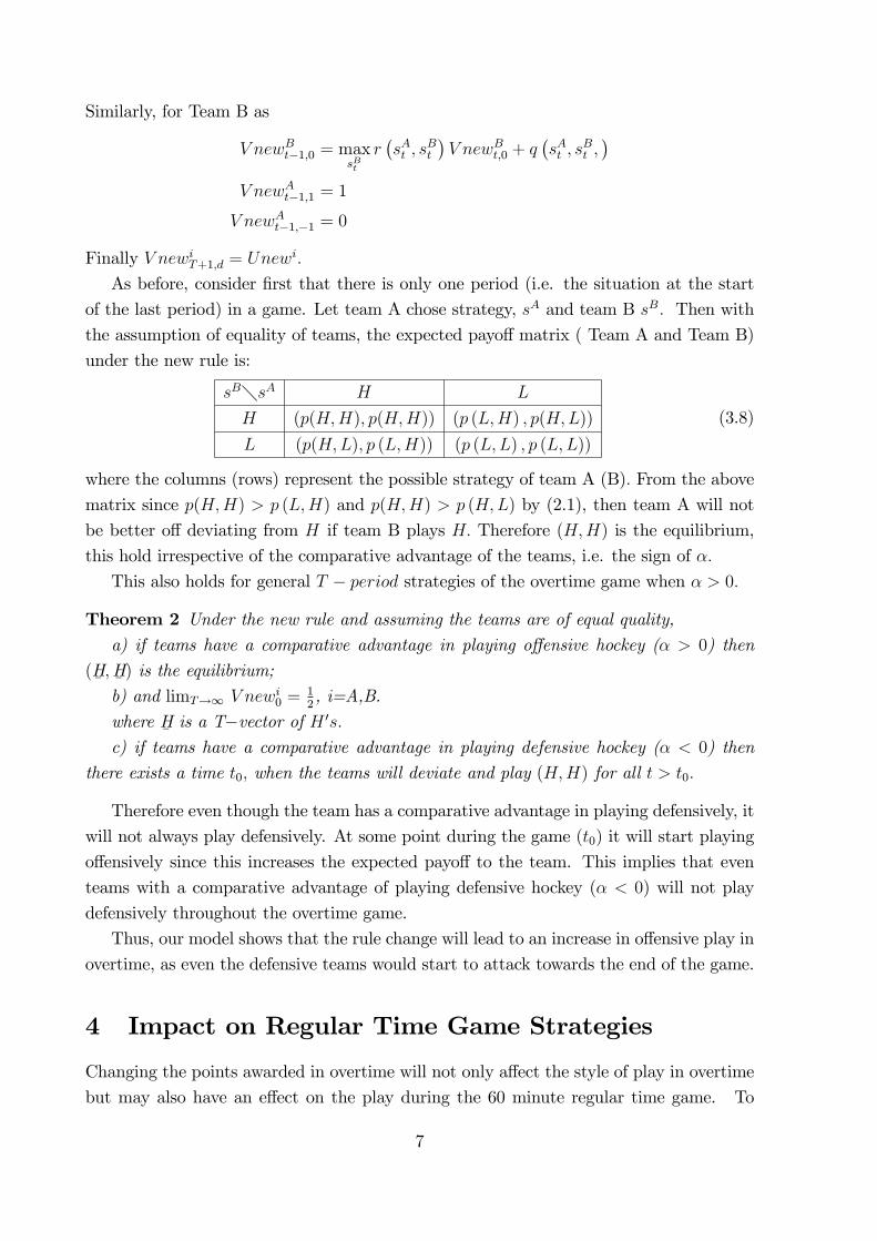
Similarly, for Team B as
V newBt�1;0 = maxsBt
r�sAt ; s
Bt
�V newBt;0 + q
�sAt ; s
Bt ;�
V newAt�1;1 = 1
V newAt�1;�1 = 0
Finally V newiT+1;d = Unewi:
As before, consider �rst that there is only one period (i.e. the situation at the start
of the last period) in a game. Let team A chose strategy, sA and team B sB: Then with
the assumption of equality of teams, the expected payo¤ matrix ( Team A and Team B)
under the new rule is:
sB�sA H L
H (p(H;H); p(H;H)) (p (L;H) ; p(H;L))
L (p(H;L); p (L;H)) (p (L;L) ; p (L;L))
(3.8)
where the columns (rows) represent the possible strategy of team A (B): From the above
matrix since p(H;H) > p (L;H) and p(H;H) > p (H;L) by (2.1), then team A will not
be better o¤ deviating from H if team B plays H: Therefore (H;H) is the equilibrium,
this hold irrespective of the comparative advantage of the teams, i.e. the sign of �:
This also holds for general T � period strategies of the overtime game when � > 0:
Theorem 2 Under the new rule and assuming the teams are of equal quality,a) if teams have a comparative advantage in playing o¤ensive hockey (� > 0) then
(H¯;H¯) is the equilibrium;
b) and limT!1 V newi0 =12, i=A,B.
where H¯is a T�vector of H 0s:
c) if teams have a comparative advantage in playing defensive hockey (� < 0) then
there exists a time t0; when the teams will deviate and play (H;H) for all t > t0:
Therefore even though the team has a comparative advantage in playing defensively, it
will not always play defensively. At some point during the game (t0) it will start playing
o¤ensively since this increases the expected payo¤ to the team. This implies that even
teams with a comparative advantage of playing defensive hockey (� < 0) will not play
defensively throughout the overtime game.
Thus, our model shows that the rule change will lead to an increase in o¤ensive play in
overtime, as even the defensive teams would start to attack towards the end of the game.
4 Impact on Regular Time Game Strategies
Changing the points awarded in overtime will not only a¤ect the style of play in overtime
but may also have an e¤ect on the play during the 60 minute regular time game. To
7
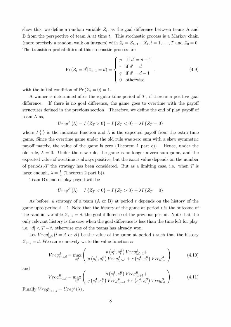
show this, we de�ne a random variable Zt; as the goal di¤erence between teams A and
B from the perspective of team A at time t: This stochastic process is a Markov chain
(more precisely a random walk on integers) with Zt = Zt�1+Xt; t = 1; : : : ; T and Z0 = 0:
The transition probabilities of this stochastic process are
Pr (Zt = d0jZt�1 = d) =
8>>><>>>:p if d0 = d+ 1
r if d0 = d
q if d0 = d� 10 otherwise
: (4.9)
with the initial condition of Pr (Z0 = 0) = 1:
A winner is determined after the regular time period of T , if there is a positive goal
di¤erence. If there is no goal di¤erence, the game goes to overtime with the payo¤
structures de�ned in the previous section. Therefore, we de�ne the end of play payo¤ of
team A as,
UregA (�) = I fZT > 0g � I fZT < 0g+ �I fZT = 0g
where I f:g is the indicator function and � is the expected payo¤ from the extra time
game. Since the overtime game under the old rule was zero sum with a skew symmetric
payo¤ matrix, the value of the game is zero (Theorem 1 part c)). Hence, under the
old rule, � = 0: Under the new rule, the game is no longer a zero sum game, and the
expected value of overtime is always positive, but the exact value depends on the number
of periods,-T the strategy has been considered. But as a limiting case, i.e. when T is
large enough, � = 12(Theorem 2 part b)).
Team B�s end of play payo¤ will be
UregB (�) = I fZT < 0g � I fZT > 0g+ �I fZT = 0g
As before, a strategy of a team (A or B) at period t depends on the history of the
game upto period t� 1: Note that the history of the game at period t is the outcome ofthe random variable Zt�1 = d, the goal di¤erence of the previous period. Note that the
only relevant history is the case when the goal di¤erence is less than the time left for play,
i.e. jdj < T � t; otherwise one of the teams has already won.Let V regit;d; (i = A or B) be the value of the game at period t such that the history
Zt�1 = d: We can recursively write the value function as
V regAt�1;d = maxsAt
p�sAt ; s
Bt
�V regAt;d+1+
q�sAt ; s
Bt
�V regAt;d�1 + r
�sAt ; s
Bt
�V regAt;d
!(4.10)
and
V regBt�1;d = maxsBt
p�sAt ; s
Bt
�V regBt;d+1+
q�sAt ; s
Bt
�V regBt;d�1 + r
�sAt ; s
Bt
�V regBt;d
!: (4.11)
Finally V regiT+1;d = Uregi (�) :
8
To demonstrate our argument that the new rule will make the teams play more defen-
sively during regulation time, all we need to show is that there will be a change of team
strategy under the new rules (for o¤ensive teams) during regulation time when the teams
are tied.
4.1 Under the old overtime rule
The overtime game under the old rule was zero sum with a skew symmetric payo¤matrix.
The value of the game is zero (Theorem 1 part c)). Hence under the old rule � = 0: Also
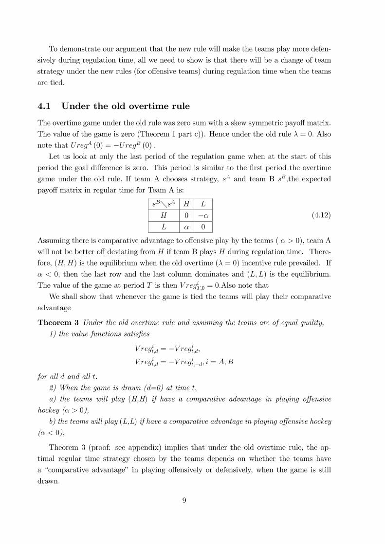
note that UregA (0) = �UregB (0) :Let us look at only the last period of the regulation game when at the start of this
period the goal di¤erence is zero. This period is similar to the �rst period the overtime
game under the old rule. If team A chooses strategy, sA and team B sB;the expected
payo¤ matrix in regular time for Team A is:
sB�sA H L
H 0 ��L � 0
(4.12)
Assuming there is comparative advantage to o¤ensive play by the teams ( � > 0), team A
will not be better o¤ deviating from H if team B plays H during regulation time. There-
fore, (H;H) is the equilibrium when the old overtime (� = 0) incentive rule prevailed. If
� < 0; then the last row and the last column dominates and (L;L) is the equilibrium.
The value of the game at period T is then V regiT;0 = 0:Also note that
We shall show that whenever the game is tied the teams will play their comparative
advantage
Theorem 3 Under the old overtime rule and assuming the teams are of equal quality,1) the value functions satis�es
V regit;d = �V regit;d;V regit;d = �V regit;�d; i = A;B
for all d and all t.
2) When the game is drawn (d=0) at time t;
a) the teams will play (H,H) if have a comparative advantage in playing o¤ensive
hockey (� > 0),
b) the teams will play (L,L) if have a comparative advantage in playing o¤ensive hockey
(� < 0),
Theorem 3 (proof: see appendix) implies that under the old overtime rule, the op-
timal regular time strategy chosen by the teams depends on whether the teams have
a �comparative advantage� in playing o¤ensively or defensively, when the game is still
drawn.
9
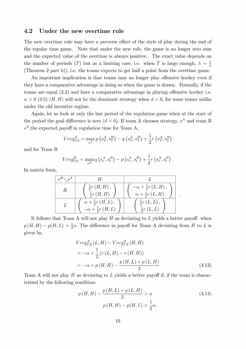
4.2 Under the new overtime rule
The new overtime rule may have a perverse e¤ect of the style of play during the end of
the regular time game. Note that under the new rule, the game is no longer zero sum
and the expected value of the overtime is always positive. The exact value depends on
the number of periods (T ) but as a limiting case, i.e. when T is large enough, � = 12
(Theorem 2 part b)), i.e. the teams expects to get half a point from the overtime game.
An important implication is that teams may no longer play o¤ensive hockey even if
they have a comparative advantage in doing so when the game is drawn. Formally, if the
teams are equal (2.2) and have a comparative advantage in playing o¤ensive hockey i.e.
� > 0 (3.5) (H;H) will not be the dominant strategy when d = 0; for some teams unlike
under the old incentive regime.
Again, let us look at only the last period of the regulation game when at the start of
the period the goal di¤erence is zero (d = 0). If team A chooses strategy, sA and team B
sB;the expected payo¤ in regulation time for Team A,
V regAT;0 = maxsAp�sAT ; s
BT
�� q
�sAT ; s
BT
�+1
2r�sAT ; s
BT
�and for Team B
V regBT;0 = maxsB
q�sAt ; s
Bt
�� p
�sAt ; s
Bt
�+1
2r�sAt ; s
Bt
�:
In matrix form,
sB�sA H L
H
12r (H;H) ;12r (H;H)
! ��+ 1
2r (L;H) ;
�+ 12r (L;H)
!
L
�+ 1
2r (H;L) ;
��+ 12r (H;L)
! 12r (L;L) ;12r (L;L)
! :
It follows that Team A will not play H as deviating to L yields a better payo¤. when
p (H;H) � p(H;L) > 12�: The di¤erence in payo¤ for Team A deviating from H to L is
given by,
V regAT;0 (L;H)� V regAT;0 (H;H)
= ��+ 12(r (L;H)� r (H;H))
= ��+ p (H;H)� p (H;L) + p (L;H)2
(4.13)
Team A will not play H as deviating to L yields a better payo¤ if, if the team is charac-
terised by the following condition:
p (H;H)� p (H;L) + p (L;H)2
> � (4.14)
p (H;H)� p(H;L) > 1
2�:
10
Similarly, Team B deviates to L:under the same conditions if the game is tied close to
the end.
This shows that under the new rule some teams (teams which satisfy condition (4.14))
at some point t0 will shift to defensive play even if their comparative advantage lies in
playing o¤ensively. Thus, the change in incentive to create more attractive play in over-
time has the perverse e¤ect of resulting in more conservative, defensive play in regulation
time (especially towards the end).
This is rational behavior for players and coaches, because why risk losing a point by
aggressively pursuing a win in regulation if the safer route is to get a regulation tie and
go for the extra point in overtime? In short, with the current rules, you can lose a game
but still get a point in the standings.
5 Empirical evidence
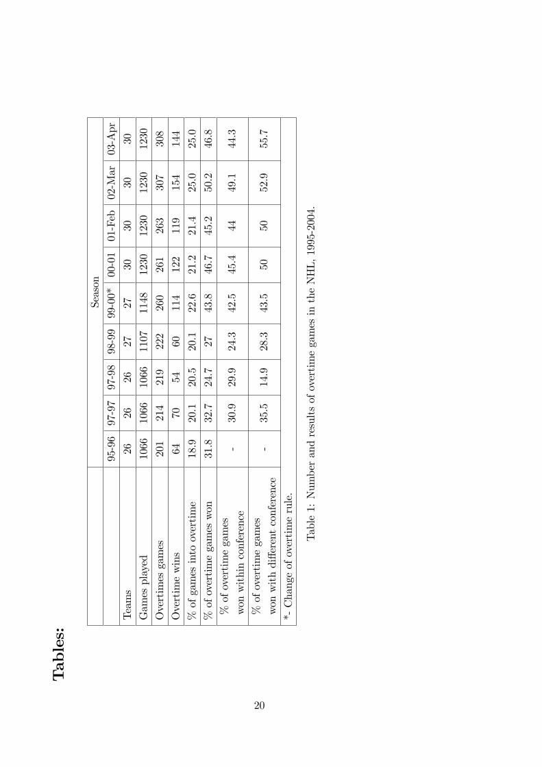
Data on the results of individual games for the last nine NHL seasons were collected
from the website http://www.hockeynut.com/archive.html. The number of regulation
and overtime games played and the results in the overtime and regulation games are
summarized in Table 1. The �rst four seasons (from the 1995-1996 season through the
1998-1999 season) represent the �old rule period�, i.e. the seasons when the losing team
in overtime game received no points while the last �ve seasons are the �new rule period�
i.e. when each team tied at the end of regulation received a single point regardless of the
outcome in overtime.
5.1 Model speci�cation
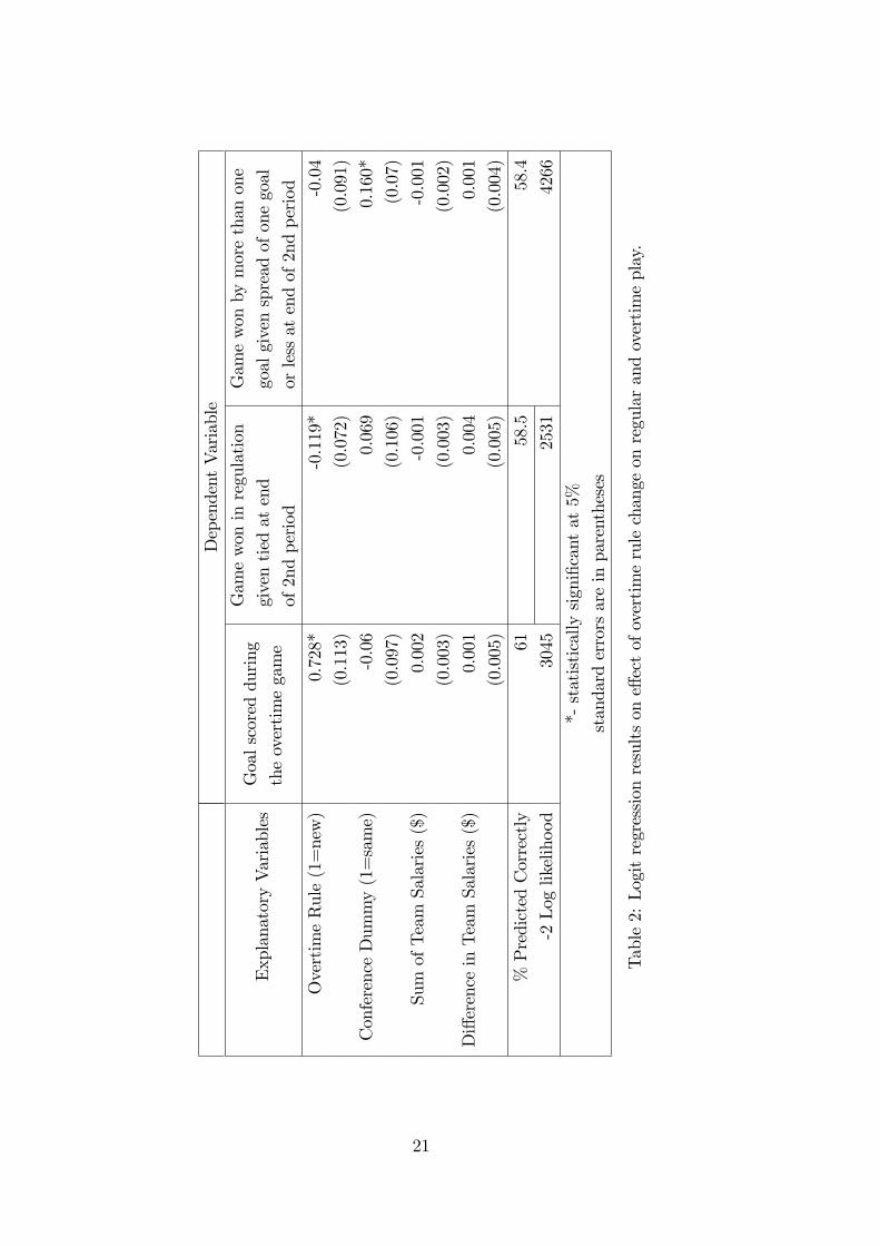
In addition to the statistical summaries in Table 1, we estimated two separate logit models
to measure the e¤ects of the rule change on the (conditional) probability of a tie in
overtime and a tie in regulation, respectively. The dependent variable in both models is
de�ned as whether there a win or a tie in the relevant period (1=win, 0=tie) �for overtime
this is identical to whether a goal was scored or not. The main explanatory variable of
concern in our study was the rule change. This variable is proxied by a dummy variable
equal to 1 for seasons with the new rule and 0 for years under the old rule.
In addition we included some variables to capture potentially important team-speci�c
or game-speci�c e¤ects. Total team payrolls and di¤erences in team salaries were used to
proxy the e¤ect of absolute and relative o¤ensive abilities by teams. Player salary informa-
tion was obtained from http://www.rodneyfort.com/PHSportsEcon/Common/OtherData
/NHLSalaries/NHLSalaries.html for the majority of the seasons and http://www.lcshockey.com
/extra/1997/salary.asp for the 1997-98 years and http://www.lcshockey.com/extra/1998/salary.asp
for the 1998-99 season. The sum of the team payrolls is assumed to increase the likelihood
11
of a goal scored and win since player salary is generally directly related to o¤ensive skills.
The absolute value of the di¤erence is also assumed to increase the chance of the game
being settled in overtime since there is a relative di¤erence in the comparative ability of
the teams to play o¤ensive hockey.
Although the theoretical model did not explicitly consider the conference of the oppo-
nent, there may be implications of conference status on team strategy. Consequently, the
conference e¤ect is included as a control variable in the empirical model. Speci�cally, a
dummy variable was included to capture the e¤ects of games played between teams within
the same or di¤erent conferences. The present 30-team NHL is divided into two confer-
ences of 15 teams (East and West). The top 8 teams within each conference make the
playo¤s at the end of the 82 game regular season. A team�s overall pro�tability is deter-
mined in large part by the revenue earned from ticket sales of home playo¤ games. Thus,
making the playo¤s generates income but so does �nishing further up the league standings
as the higher placed team earns home-ice advantage in any playo¤ series. Thus, incentives
and correspondingly team strategy in overtime may vary depending upon whether the op-
ponent is from the same conference. Since relative positions determine playo¤ ranking
and potential home-ice advantage, teams within the same conference may wish to avoid
giving an additional point in overtime to their opponents. While teams from within the
same conference could gain from an additional point in overtime, the consequences of giv-
ing up a goal are signi�cant. In contrast, both teams have nothing to lose by attempting
to score in overtime if they are in di¤erent conferences.
5.2 Regression results
The averages in Table 1 and the logit regression results in Table 2 are consistent with
the predictions from our model on overtime team behavior, i.e. that teams take a more
o¤ensive approach in overtime if both teams are guaranteed a single point going into the
overtime: (Theorem 1 and 2). If a team could lose a point by giving up a goal in the
5 minute overtime, teams would play a conservative strategy to avoid losing what they
had gained over the 60 minutes of regulation play. Table 1 shows how under the old rule
period, on average 71% of the games tied in regulation remained tied during overtime. In
contrast, under the new rule, only 53% of the games tied after regulation remained tied in
overtime. Moreover, the numbers are fairly constant for the various seasons within both
the old rule and the new rule period, suggesting a clear structural e¤ect on overtime team
strategies.
However, there is a potential causality problem with this interpretation of the em-
pirical evidence on overtime strategies. The modi�cation to the NHL overtime rule at
the beginning of the 1999-2000 season not only changed the point system but also the
number of skaters on the ice. In order to further increase the possibility of scoring, the
12
NHL went from the 5-on-5 play used in regulation time to 4-on-4. Since both the point
system and number of players for overtime were changed at the same time, the e¤ect of
each on the signi�cant increase in overtime wins cannot be determined. However, Abre-
vaya (2002) gathered overtime results for the American Hockey League (AHL) which is
a minor league a¢ liate of the NHL. The two overtime rule changes were implemented
separately by the AHL. The data indicate that the awarding a single point in overtime
was primarily responsible for the increased number of overtime wins. Prior to the rule
change, 68% of overtime games remained tied and this dropped to 59% with the change
in point system. The percentage dropped slightly further to 55% with the introduction
of 4-on-4 play. Thus, the scoring system change has increased the likelihood of o¤ensive
strategy in overtime as desired.
The other explanatory variables on the probability of a win in overtime were statis-
tically insigni�cant but were of the expected signs (column 2 of Table 2). Teams from
within the same conference are less likely to score in overtime. In addition, games involv-
ing high payroll teams and ones with a large spread in team salaries are more likely to be
involved in overtime game that results in a win for one team.
While the overtime rule change had the desired positive e¤ect on play in overtime, the
empirical results con�rm the unintended consequences of the point change on regular time
play. Theorem 3 predicts that the overtime rule changes would lead to more defensive play
during regulation. The hypothesized e¤ect is consistent with summary measures presented
in Table 1. The percentage of games ending in a tie after the 60 minute regulation time
increased from on average 20.2% to 23.1% with the change in the overtime payo¤structure.
To measure whether the overtime rule change a¤ected regular time play, we focus
speci�cally on play in the third period. The logit regression in Table 2 measures the
likelihood that the game remained tied, given that the game was tied with one period
remaining. Our theory would suggest conservative play would dominate in the 3rd period
leading to a greater chance of a tie game at the end. The regression results in the third
column of Table 2 show that the change in the overtime rule indeed signi�cantly reduced
the likelihood of one team winning at the end of regulation given the game was tied with
one period remaining. The other variables have the expected e¤ects : conservative play
in the 3rd period is more likely between teams of the same conference and teams with
lower payrolls (both total and absolute di¤erence). However, none of these e¤ects are
statistically signi�cant.
The e¤ect of the overtime rule change on play during regulation time was also assessed
in terms of the likelihood of the goal spread increasing rather than staying the same. A
third logit regression (column 4 in Table 2) estimated how the rule change a¤ected the
likelihood of the goal spread changing in the last period. Across the nine seasons, teams
were separated by one goal at the end of the 2nd period in 38% of the games and there
was no signi�cant di¤erence before and after the overtime rule change. Given the one goal
13
di¤erence, the spread increased to two or more goals in approximately 40% of the games.
The logit regression results in Table 2 show that there was no signi�cant impact of
the rule change on the goal spread. The overtime rule change has no impact on scoring in
games with a one goal spread at the end of the 2nd period since both before and after the
rule change the team with the lead will attempt to protect the lead and play defensively
while the team behind will attempt to close the gag and play o¤ensively. This result is not
inconsistent with the previous �nding that teams in a close game are more likely to remain
tied at the end of regulation play under the new overtime point scheme. In a one-goal
game, the team ahead will likely to decide to play defensively and wait to counter-attack
against a team pressing to score the equalizer. However, an o¤ensive team seeking to
increase its one goal lead may also expose itself and be more vulnerable to letting in a
tying goal. Thus, the hypothesized conservative regulation play during regulation under
the overtime rule change is likely to lead to games tied near the end remaining tight but
have an ambiguous e¤ect on games separated by one goal at the end of the 2nd period.
Table 1
Table 2
6 Increasing rewards for a win in the regular time
Another contemplated change to the incentives facing NHL teams is to give a winning
team three points for a regulation win as opposed to two. Such a change in the point
structure has been implemented in most professional soccer leagues. One version of the
reward system would give a team three points for a win in regulation, two for a win in
overtime, one for a tie or an overtime loss, and zero for a loss in regulation. The intent of
such a change is to create a more attacking style of game since teams would be rewarded
for doing better and trying to win in regulation rather than play conservatively and settle
for a guaranteed one point arising from a tie in regulation (Mullin, J (2003)).
To analyze how such a proposed rule change would a¤ect team strategies, we will use
the model developed above. We de�ne the end of play payo¤ UregA of team A as,
UnewregA = 2I fZT > 0g � I fZT < 0g+1
2I fZT = 0g (6.15)
where I f:g is the indicator function and the expected payo¤ from tieing a regulation timegame is 1
2:
Team B�s end of play payo¤ will be
UnewregB = 2I fZT < 0g � I fZT > 0g+1
2I fZT = 0g (6.16)
14
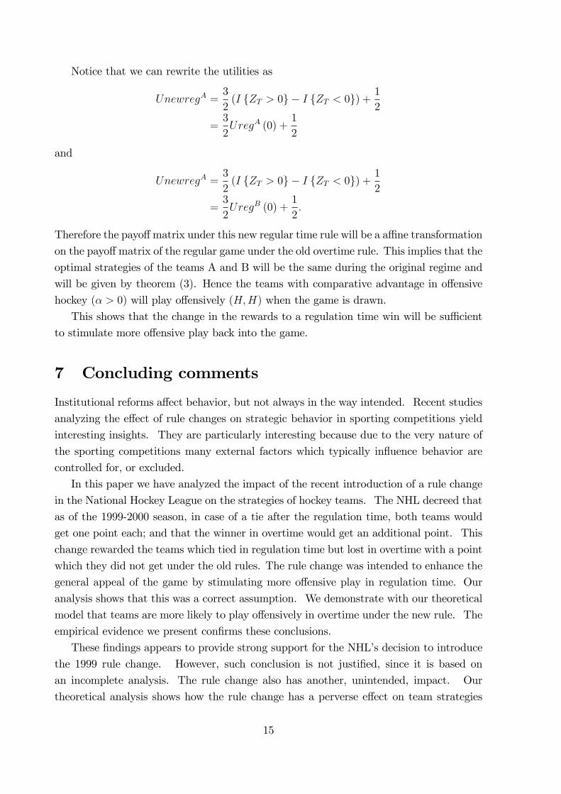
Notice that we can rewrite the utilities as
UnewregA =3
2(I fZT > 0g � I fZT < 0g) +
1
2
=3
2UregA (0) +
1
2
and
UnewregA =3
2(I fZT > 0g � I fZT < 0g) +
1
2
=3
2UregB (0) +
1
2:
Therefore the payo¤matrix under this new regular time rule will be a a¢ ne transformation
on the payo¤matrix of the regular game under the old overtime rule. This implies that the
optimal strategies of the teams A and B will be the same during the original regime and
will be given by theorem (3). Hence the teams with comparative advantage in o¤ensive
hockey (� > 0) will play o¤ensively (H;H) when the game is drawn.
This shows that the change in the rewards to a regulation time win will be su¢ cient
to stimulate more o¤ensive play back into the game.
7 Concluding comments
Institutional reforms a¤ect behavior, but not always in the way intended. Recent studies
analyzing the e¤ect of rule changes on strategic behavior in sporting competitions yield
interesting insights. They are particularly interesting because due to the very nature of
the sporting competitions many external factors which typically in�uence behavior are
controlled for, or excluded.
In this paper we have analyzed the impact of the recent introduction of a rule change
in the National Hockey League on the strategies of hockey teams. The NHL decreed that
as of the 1999-2000 season, in case of a tie after the regulation time, both teams would
get one point each; and that the winner in overtime would get an additional point. This
change rewarded the teams which tied in regulation time but lost in overtime with a point
which they did not get under the old rules. The rule change was intended to enhance the
general appeal of the game by stimulating more o¤ensive play in regulation time. Our
analysis shows that this was a correct assumption. We demonstrate with our theoretical
model that teams are more likely to play o¤ensively in overtime under the new rule. The
empirical evidence we present con�rms these conclusions.
These �ndings appears to provide strong support for the NHL�s decision to introduce
the 1999 rule change. However, such conclusion is not justi�ed, since it is based on
an incomplete analysis. The rule change also has another, unintended, impact. Our
theoretical analysis shows how the rule change has a perverse e¤ect on team strategies
15
in regulation time, causing more defensive play during the main part of the game. The
empirical evidence provides support for this conclusion. Hence the conclusions based on
the full e¤ects of the rule change should be less positive, and more nuanced.
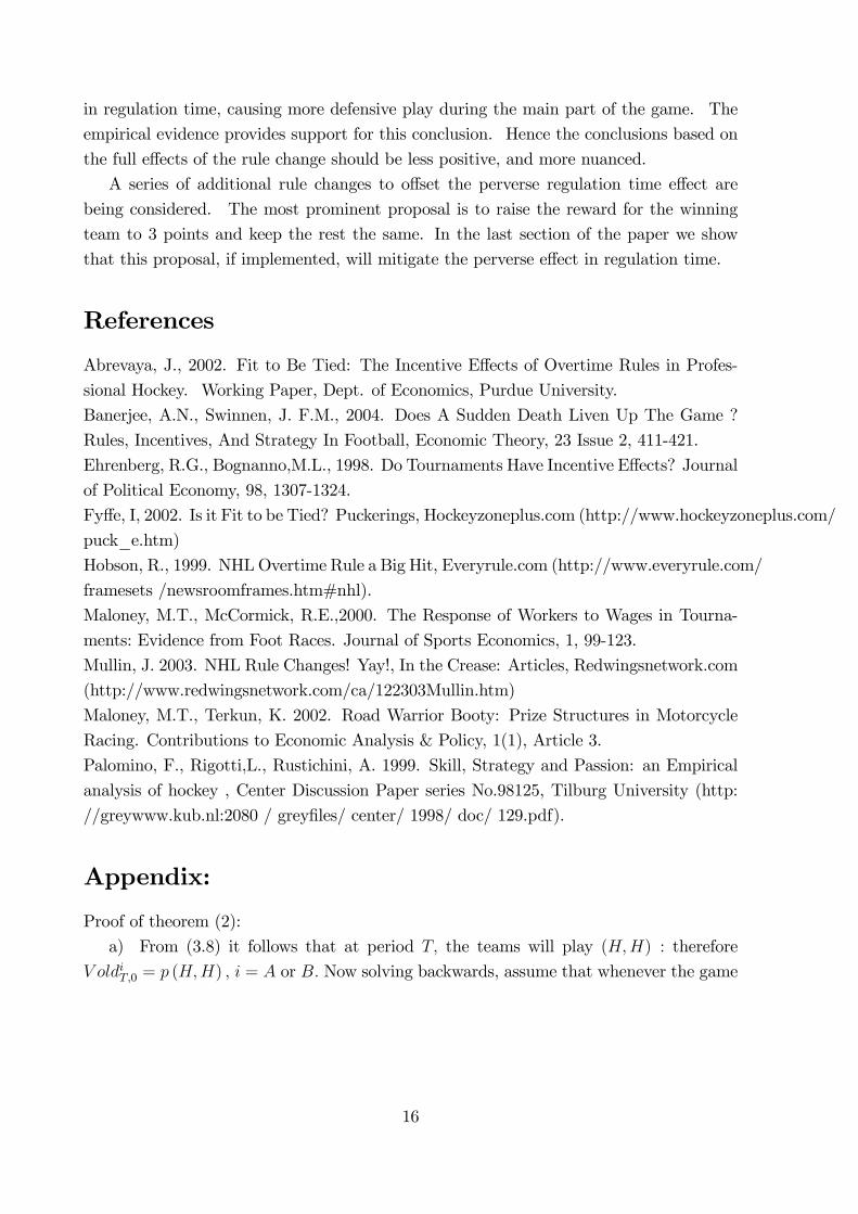
A series of additional rule changes to o¤set the perverse regulation time e¤ect are
being considered. The most prominent proposal is to raise the reward for the winning
team to 3 points and keep the rest the same. In the last section of the paper we show
that this proposal, if implemented, will mitigate the perverse e¤ect in regulation time.
References
Abrevaya, J., 2002. Fit to Be Tied: The Incentive E¤ects of Overtime Rules in Profes-
sional Hockey. Working Paper, Dept. of Economics, Purdue University.
Banerjee, A.N., Swinnen, J. F.M., 2004. Does A Sudden Death Liven Up The Game ?
Rules, Incentives, And Strategy In Football, Economic Theory, 23 Issue 2, 411-421.
Ehrenberg, R.G., Bognanno,M.L., 1998. Do Tournaments Have Incentive E¤ects? Journal
of Political Economy, 98, 1307-1324.
Fy¤e, I, 2002. Is it Fit to be Tied? Puckerings, Hockeyzoneplus.com (http://www.hockeyzoneplus.com/
puck_e.htm)
Hobson, R., 1999. NHLOvertime Rule a Big Hit, Everyrule.com (http://www.everyrule.com/
framesets /newsroomframes.htm#nhl).
Maloney, M.T., McCormick, R.E.,2000. The Response of Workers to Wages in Tourna-
ments: Evidence from Foot Races. Journal of Sports Economics, 1, 99-123.
Mullin, J. 2003. NHL Rule Changes! Yay!, In the Crease: Articles, Redwingsnetwork.com
(http://www.redwingsnetwork.com/ca/122303Mullin.htm)
Maloney, M.T., Terkun, K. 2002. Road Warrior Booty: Prize Structures in Motorcycle
Racing. Contributions to Economic Analysis & Policy, 1(1), Article 3.
Palomino, F., Rigotti,L., Rustichini, A. 1999. Skill, Strategy and Passion: an Empirical
analysis of hockey , Center Discussion Paper series No.98125, Tilburg University (http:
//greywww.kub.nl:2080 / grey�les/ center/ 1998/ doc/ 129.pdf).
Appendix:
Proof of theorem (2):
a) From (3.8) it follows that at period T; the teams will play (H;H) : therefore
V oldiT;0 = p (H;H) ; i = A or B: Now solving backwards, assume that whenever the game
16
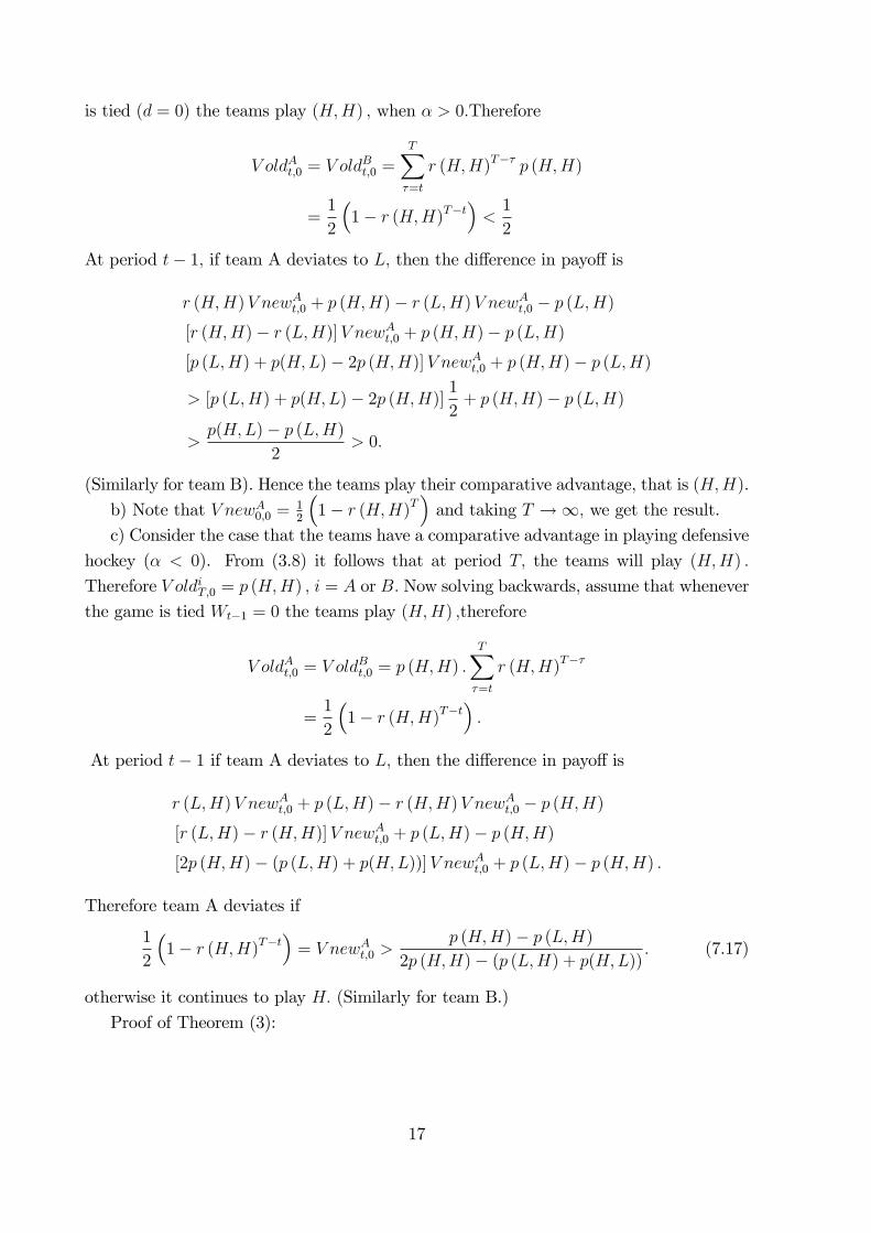
is tied (d = 0) the teams play (H;H) ; when � > 0:Therefore
V oldAt;0 = V oldBt;0 =
TX�=t
r (H;H)T�� p (H;H)
=1
2
�1� r (H;H)T�t
�<1
2
At period t� 1; if team A deviates to L; then the di¤erence in payo¤ is
r (H;H)V newAt;0 + p (H;H)� r (L;H)V newAt;0 � p (L;H)[r (H;H)� r (L;H)]V newAt;0 + p (H;H)� p (L;H)[p (L;H) + p(H;L)� 2p (H;H)]V newAt;0 + p (H;H)� p (L;H)
> [p (L;H) + p(H;L)� 2p (H;H)] 12+ p (H;H)� p (L;H)
>p(H;L)� p (L;H)
2> 0:
(Similarly for team B). Hence the teams play their comparative advantage, that is (H;H).
b) Note that V newA0;0 =12
�1� r (H;H)T
�and taking T !1; we get the result.
c) Consider the case that the teams have a comparative advantage in playing defensive
hockey (� < 0). From (3.8) it follows that at period T; the teams will play (H;H) :
Therefore V oldiT;0 = p (H;H) ; i = A or B: Now solving backwards, assume that whenever
the game is tied Wt�1 = 0 the teams play (H;H) ;therefore
V oldAt;0 = V oldBt;0 = p (H;H) :
TX�=t
r (H;H)T��
=1
2
�1� r (H;H)T�t
�:
At period t� 1 if team A deviates to L; then the di¤erence in payo¤ is
r (L;H)V newAt;0 + p (L;H)� r (H;H)V newAt;0 � p (H;H)[r (L;H)� r (H;H)]V newAt;0 + p (L;H)� p (H;H)[2p (H;H)� (p (L;H) + p(H;L))]V newAt;0 + p (L;H)� p (H;H) :
Therefore team A deviates if
1
2
�1� r (H;H)T�t
�= V newAt;0 >
p (H;H)� p (L;H)2p (H;H)� (p (L;H) + p(H;L)) : (7.17)
otherwise it continues to play H: (Similarly for team B.)
Proof of Theorem (3):
17
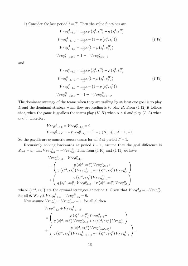
1) Consider the last period t = T: Then the value functions are
V regAT�1;0 = maxsAp�sAt ; s
Bt
�� q
�sAt ; s
Bt
�V regAT�1;�1 = max
sA��1� p
�sAt ; s
Bt
��(7.18)
V regAT�1;1 = maxsA
�1� p
�sAt ; s
Bt
��V regAT�1;d>1 = 1 = �V regAT;d<�1
and
V regBT�1;0 = maxsB
q�sAt ; s
Bt
�� p
�sAt ; s
Bt
�V regBT�1;�1 = max
sB
�1� p
�sAt ; s
Bt
��(7.19)
V regBT�1;1 = maxsB
��1� p
�sAt ; s
Bt
��V regBT�1;d>1 = �1 = �V regBT;d<�1:
The dominant strategy of the teams when they are trailing by at least one goal is to play
L and the dominant strategy when they are leading is to play H: From (4.12) it follows
that, when the game is goalless the teams play (H;H) when � > 0 and play (L;L) when
� < 0: Therefore
V regAT�1;0 = V regBT�1;0 = 0
V regAT�1;d = �V regBT�1;d = (1� p (H;L)) ; d = 1;�1:
So the payo¤s are symmetric across teams for all d at period T � 1:Recursively solving backwards at period t � 1; assume that the goal di¤erence is
Zt�1 = d, and V regAt;;d = �V regBt;d; Then from (4.10) and (4.11) we have
V regAt�1;d + V regBt�1;d
=
p�s�At ; s�Bt
�V regAt;d+1+
q�s�At ; s�Bt
�V regAt;d�1 + r
�s�At ; s�Bt
�V regAt;d
!
+
p�s�At ; s�Bt
�V regBt;d+1+
q�s�At ; s�Bt
�V regBt;d�1 + r
�s�At ; s�Bt
�V regBt;d
!where
�s�At ; s�Bt
�are the optimal strategies at period t: Given that V regAt;;d = �V regBt;d;
for all d: We get V regAt�1;d + V regBt�1;d = 0:
Now assume V regAt;d + V regAt;�d = 0; for all d; then
V regAt�1;d + V regAt�1;�d
=
p�s�At ; s�Bt
�V regAt;d+1+
q�s�At ; s�Bt
�V regAt;d�1 + r
�s�At ; s�Bt
�V regAt;d
!
+
p�s�At ; s�Bt
�V regAt;�(d�1)+
q�s�At ; s�Bt
�V regAt;�(d+1) + r
�s�At ; s�Bt
�V regAt;�d
!:
18
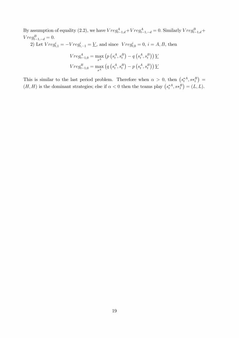
By assumption of equality (2.2), we have V regAt�1;d+V regAt�1;�d = 0: Similarly V reg
Bt�1;d+
V regBt�1;�d = 0:
2) Let V regit;1 = �V regit;�1 = V ; and since V regit;0 = 0; i = A;B, then
V regAt�1;0 = maxsA
�p�sAt ; s
Bt
�� q
�sAt ; s
Bt
��V
V regBt�1;0 = maxsA
�q�sAt ; s
Bt
�� p
�sAt ; s
Bt
��V
This is similar to the last period problem. Therefore when � > 0; then�s�At ; s�Bt
�=
(H;H) is the dominant strategies; else if � < 0 then the teams play�s�At ; s�Bt
�= (L;L).
19
Tables:
Season
95-9697-9797-9898-9999-00*
00-0101-Feb
02-Mar
03-Apr
Teams
2626
2627
2730
3030
30
Gamesplayed
1066
1066
1066
1107
1148
1230
1230
1230
1230
Overtimesgames
201
214
219
222
260
261
263
307
308
Overtimewins
6470
5460
114
122
119
154
144
%ofgamesintoovertime
18.9
20.1
20.5
20.1
22.6
21.2
21.4
25.0
25.0
%ofovertimegameswon
31.8
32.7
24.7
2743.8
46.7
45.2
50.2
46.8
%ofovertimegames
wonwithinconference
-30.9
29.9
24.3
42.5
45.4
4449.1
44.3
%ofovertimegames
wonwithdi¤erentconference
-35.5
14.9
28.3
43.5
5050
52.9
55.7
*-Changeofovertimerule.
Table1:NumberandresultsofovertimegamesintheNHL,1995-2004.
20
DependentVariable
ExplanatoryVariables
Goalscoredduring
theovertimegame
Gamewoninregulation
giventiedatend
of2ndperiod
Gamewonbymorethanone
goalgivenspreadofonegoal
orlessatendof2ndperiod
OvertimeRule(1=new)
0.728*
-0.119*
-0.04
(0.113)
(0.072)
(0.091)
ConferenceDummy(1=same)
-0.06
0.069
0.160*
(0.097)
(0.106)
(0.07)
SumofTeamSalaries($)
0.002
-0.001
-0.001
(0.003)
(0.003)
(0.002)
Di¤erenceinTeamSalaries($)
0.001
0.004
0.001
(0.005)
(0.005)
(0.004)
%PredictedCorrectly
6158.5
58.4
-2Loglikelihood
3045
2531
4266
*-statisticallysigni�cantat5%
standarderrorsareinparentheses
Table2:Logitregressionresultsone¤ectofovertimerulechangeonregularandovertimeplay.
21