Embed Size (px)
Citation preview
EC 324: Macroeconomics (Advanced)Consumption
Nicole Kuschy
January 17, 2011

Course Organization
Contact time:
Lectures: Monday, 15:00-16:00Friday, 10:00-11:00
Class: Thursday, 13:00-14:00 (week 17-25)
Course supervisor: Nicole Kuschy
Email: [email protected]
Office hours: Monday, 16:00-18:00

Assessment
Coursework:
mid-term on Friday 25th of February, 17:00
Exam:
2 hours, during the summer term
Final mark: Whichever is the greater:
EITHER 50% coursework mark, 50% exam markOR 100% exam mark
Details in Undergraduate Economics Handbook.

Reading
Textbook:
Sørensen, Peter Birch and Hans Jørgen Whitta-Jacobsen(2010): Introducing Advanced Macroeconomics: Growthand Business Cycles, McGraw-Hill. (SWJ)
Supplementary readings:
Romer, David (2006): Advanced Macroeconomics, 3rdEdition, McGraw-Hill.Journal articles as indicated.
Lecture notes and additional material posted on the CMR.
Agenda I
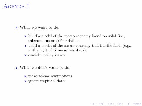
What we want to do:
build a model of the macro economy based on solid (i.e.,microeconomic) foundations
build a model of the macro economy that fits the facts (e.g.,in the light of time-series data)
consider policy issues
What we don’t want to do:
make ad-hoc assumptions
ignore empirical data

Agenda II
1 Consumption
2 Investment
3 Monetary Policy Rules
4 Incomplete Nominal Adjustment
5 The Phillips Curve
6 An Empirical AD/AS Model
7 Rational Expectations and Policy Ineffectiveness
8 Credibility and Policy Making
9 Delegation
Lecture 1: Consumption
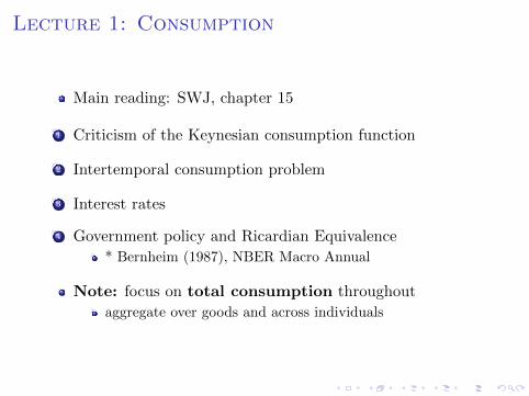
Main reading: SWJ, chapter 15
1 Criticism of the Keynesian consumption function
2 Intertemporal consumption problem
3 Interest rates
4 Government policy and Ricardian Equivalence
* Bernheim (1987), NBER Macro Annual
Note: focus on total consumption throughout
aggregate over goods and across individuals
Keynesian Consumption Function (KCF)
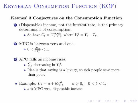
Keynes’ 3 Conjectures on the Consumption Function
1 (Disposable) income, not the interest rate, is the primarydeterminant of consumption.
So have Ct = C(Y dt ), where Y dt = Yt − Tt.
2 MPC is between zero and one.
0 < dCtdY dt
< 1.
3 APC falls as income rises.CtY dt
decreasing in Y dt .
Idea is that saving is a luxury, so rich people save morethan poor.
Example: Ct = a+ bY dt , a > 0, 0 < b < 1.
b is MPC wrt. disposable income
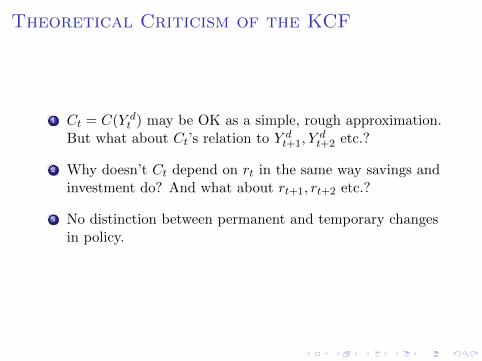
Theoretical Criticism of the KCF
1 Ct = C(Y dt ) may be OK as a simple, rough approximation.
But what about Ct’s relation to Y dt+1, Y
dt+2 etc.?
2 Why doesn’t Ct depend on rt in the same way savings andinvestment do? And what about rt+1, rt+2 etc.?
3 No distinction between permanent and temporary changesin policy.
Empirical Criticism of the KCF
Slide 1/1©The McGraw-Hill Companies, 2005
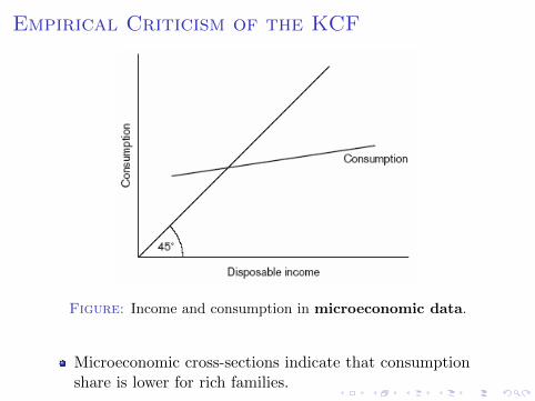
Figure 16.1a: Stylized relationship between income and consumption in microeconomic cross-section data
Figure: Income and consumption in microeconomic data.
Microeconomic cross-sections indicate that consumptionshare is lower for rich families.
Empirical Criticism of the KCF
Slide 1/2©The McGraw-Hill Companies, 2005
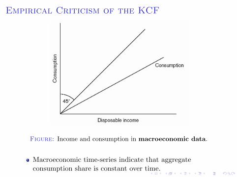
Figure 16.1b: Stylized relationship between income and consumption in macroeconomic time series data
Figure: Income and consumption in macroeconomic data.
Macroeconomic time-series indicate that aggregateconsumption share is constant over time.
Empirical Criticism of the KCF
Slide 1/3©The McGraw-Hill Companies, 2005
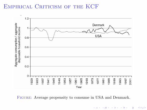
Figure 16.2: The average propensity to consume in USA and Denmark
.
Source: National Income Accounts, Bureau of Economic Analysis and ADAM database, Statistics Denmark
Figure: Average propensity to consume in USA and Denmark.
Empirical Criticism of the KCF
Conclusion:
KCF unsatisfactory
need a more developed model
We focus on the Permanent Income Hypothesis (PIH);the idea is that individuals make consumption/savingsdecisions across time, i.e., intertemporal choice.
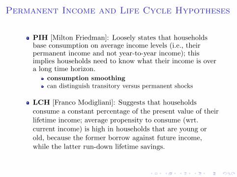
Permanent Income and Life Cycle Hypotheses
PIH [Milton Friedman]: Loosely states that householdsbase consumption on average income levels (i.e., theirpermanent income and not year-to-year income); thisimplies households need to know what their income is overa long time horizon.
consumption smoothingcan distinguish transitory versus permanent shocks
LCH [Franco Modigliani]: Suggests that householdsconsume a constant percentage of the present value of theirlifetime income; average propensity to consume (wrt.current income) is high in households that are young orold, because the former borrow against future income,while the latter run-down lifetime savings.
Intertemporal Consumption ProblemSetup
A Two-Period Endowment Economy
Households are ‘alive’ for two periods, t = 1, 2{today, tomorrow}.
There is a single good, Yt.
Perfect capital markets: Households borrow and lend atthe same market interest rate, r.
No uncertainty.

Intertemporal Consumption ProblemConsumer Preferences
Household maximizes lifetime (t = 1, 2) utility, U :
U = u(C1) + βu(C2) (1)
β ∈ (0, 1) is a fixed subjective discount factor (sometimescalled private discount factor) measuring the impatienceto consume.
Aside: SWJ put 11+φ rather than β.
Ct is consumption at time t.
u is the period utility function, with u (C)′ > 0 andu (C)′′ < 0.
Implication: Desire to smooth consumption.
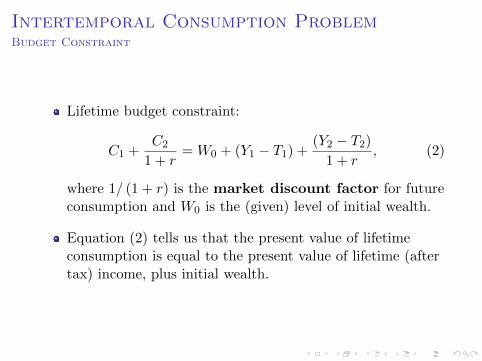
Intertemporal Consumption ProblemBudget Constraint
Lifetime budget constraint:
C1 +C2
1 + r= W0 + (Y1 − T1) +
(Y2 − T2)1 + r
, (2)
where 1/ (1 + r) is the market discount factor for futureconsumption and W0 is the (given) level of initial wealth.
Equation (2) tells us that the present value of lifetimeconsumption is equal to the present value of lifetime (aftertax) income, plus initial wealth.
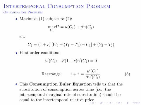
Intertemporal Consumption ProblemOptimization Problem
Maximize (1) subject to (2):
maxC1
U = u(C1) + βu(C2)
s.t.
C2 = (1 + r) [W0 + (Y1 − T1)− C1] + (Y2 − T2)
First order condition:
u′(C1)− β(1 + r)u′(C2) = 0
Rearrange: 1 + r =u′(C1)
βu′(C2)(3)
This Consumption Euler Equation tells us that thesubstitution of consumption across time (i.e., theintertemporal marginal rate of substitution) should beequal to the intertemporal relative price.

Intertemporal Consumption ProblemEquilibrium Allocation
Slide 1/4©The McGraw-Hill Companies, 2005
Figure 16.3: The consumer’s optimal intertemporal allocationof consumption
Figure: Optimal intertemporal allocation of consumption.
Intertemporal Consumption ProblemEquilibrium Allocation
Budget constraint:
C1 +C2
1 + r= W0 + (Y1 − T1) +
(Y2 − T2)1 + r
totally differentiate to derive the slope:
dC1 +dC2
1 + r= 0 ⇐⇒ dC2
dC1= −(1 + r)
Indifference curve:
U = u(C1) + βu(C2) = const.
totally differentiate to derive the slope:
dU = u′(C1)dC1 + βu′(C2)dC2 = 0 ⇐⇒ dC2
dC1= − u′(C1)
βu′(C2)
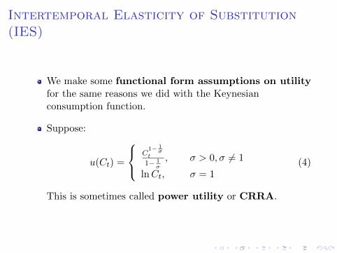
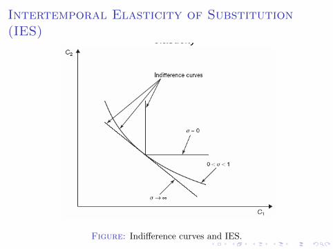
Intertemporal Elasticity of Substitution(IES)
We make some functional form assumptions on utilityfor the same reasons we did with the Keynesianconsumption function.
Suppose:
u(Ct) =
C1− 1
σt
1− 1σ
, σ > 0, σ 6= 1
lnCt, σ = 1(4)
This is sometimes called power utility or CRRA.
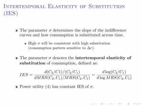
Intertemporal Elasticity of Substitution(IES)
The parameter σ determines the slope of the indifferencecurves and how consumption is substituted across time.
High σ will be consistent with high substitution(consumption pattern sensitive to ∆r).
The parameter σ denotes the intertemporal elasticity ofsubstitution of consumption, defined as:
IES =d(C2/C1)/(C2/C1)
dMRS(C2, C1)/MRS(C2, C1)=
d log(C2/C1)
d logMRS(C2, C1)
Power utility (4) has constant IES of σ.
Intertemporal Elasticity of Substitution(IES)
Slide 1/9©The McGraw-Hill Companies, 2005
Figure 16.7: The relation between the shape of the indifference curve and the intertemporal substitution
elasticity
Figure: Indifference curves and IES.
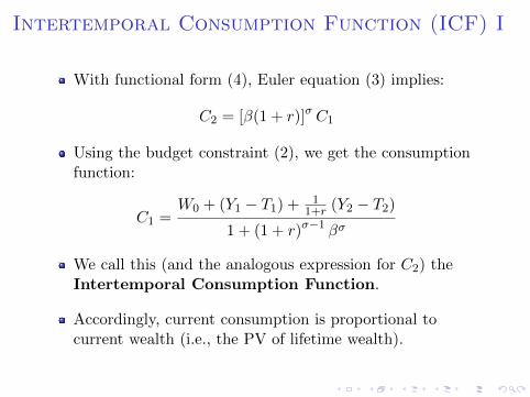
Intertemporal Consumption Function (ICF) I
With functional form (4), Euler equation (3) implies:
C2 = [β(1 + r)]σ C1
Using the budget constraint (2), we get the consumptionfunction:
C1 =W0 + (Y1 − T1) + 1
1+r (Y2 − T2)1 + (1 + r)σ−1 βσ
We call this (and the analogous expression for C2) theIntertemporal Consumption Function.
Accordingly, current consumption is proportional tocurrent wealth (i.e., the PV of lifetime wealth).
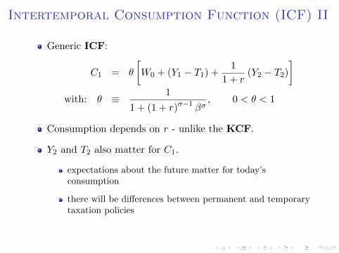
Intertemporal Consumption Function (ICF) II
Generic ICF:
C1 = θ
[W0 + (Y1 − T1) +
1
1 + r(Y2 − T2)
]with: θ ≡ 1
1 + (1 + r)σ−1 βσ, 0 < θ < 1
Consumption depends on r - unlike the KCF.
Y2 and T2 also matter for C1.
expectations about the future matter for today’sconsumption
there will be differences between permanent and temporarytaxation policies
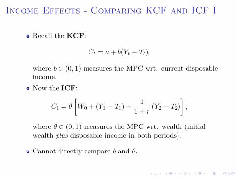
Income Effects - Comparing KCF and ICF I
Recall the KCF:
Ct = a+ b(Yt − Tt),
where b ∈ (0, 1) measures the MPC wrt. current disposableincome.
Now the ICF:
C1 = θ
[W0 + (Y1 − T1) +
1
1 + r(Y2 − T2)
],
where θ ∈ (0, 1) measures the MPC wrt. wealth (initialwealth plus disposable income in both periods).
Cannot directly compare b and θ.
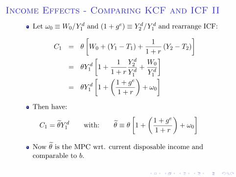
Income Effects - Comparing KCF and ICF II
Let ω0 ≡W0/Yd1 and (1 + ge) ≡ Y d
2 /Yd1 and rearrange ICF:
C1 = θ
[W0 + (Y1 − T1) +
1
1 + r(Y2 − T2)
]= θY d
1
[1 +
1
1 + r
Y d2
Y d1
+W0
Y d1
]= θY d
1
[1 +
(1 + ge
1 + r
)+ ω0
]Then have:
C1 = θ̃Y d1 with: θ̃ ≡ θ
[1 +
(1 + ge
1 + r
)+ ω0
]Now θ̃ is the MPC wrt. current disposable income andcomparable to b.
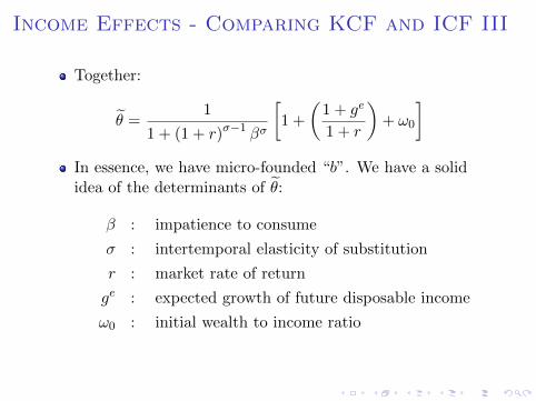
Income Effects - Comparing KCF and ICF III
Together:
θ̃ =1
1 + (1 + r)σ−1 βσ
[1 +
(1 + ge
1 + r
)+ ω0
]In essence, we have micro-founded “b”. We have a solididea of the determinants of θ̃:
β : impatience to consume
σ : intertemporal elasticity of substitution
r : market rate of return
ge : expected growth of future disposable income
ω0 : initial wealth to income ratio
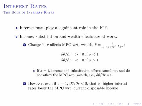
Interest RatesThe Role of Interest Rates
Interest rates play a significant role in the ICF.
Income, substitution and wealth effects are at work.
1 Change in r affects MPC wrt. wealth, θ = 11+(1+r)σ−1βσ
:
∂θ/∂r > 0 if σ < 1
∂θ/∂r < 0 if σ > 1
If σ = 1, income and substitution effects cancel out and donot affect the MPC wrt. wealth, i.e., ∂θ/∂r = 0.
2 However, even if σ = 1, ∂θ̃/∂r < 0; that is, higher interestrates lower the MPC wrt. current disposable income.
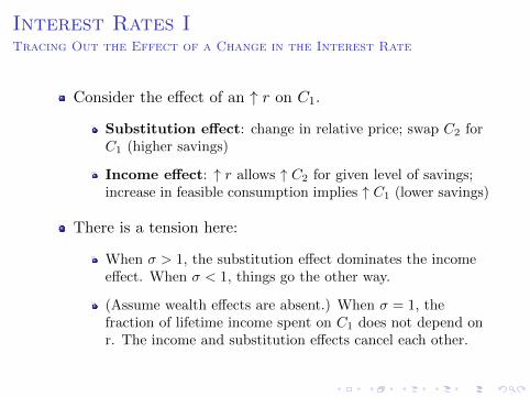
Interest Rates ITracing Out the Effect of a Change in the Interest Rate
Consider the effect of an ↑ r on C1.
Substitution effect: change in relative price; swap C2 forC1 (higher savings)
Income effect: ↑ r allows ↑ C2 for given level of savings;increase in feasible consumption implies ↑ C1 (lower savings)
There is a tension here:
When σ > 1, the substitution effect dominates the incomeeffect. When σ < 1, things go the other way.
(Assume wealth effects are absent.) When σ = 1, thefraction of lifetime income spent on C1 does not depend onr. The income and substitution effects cancel each other.
Interest Rates IITracing Out the Effect of a Change in the Interest Rate
Interest rates and savings in the two-period case
Assume: W0 = 0, i.e., no initial wealth
Three cases:
1 zero initial savings
2 positive initial savings (individual is net saver)
3 negative initial savings (individual is net borrower)
Graphical illustration
see Romer (2006), chapter 7.4
Interest Rates IIITracing Out the Effect of a Change in the Interest Rate
In addition to income and substitution effects, there maybe a wealth effect.
Most transparant case is when σ = 1 (since then know thatincome and substitution effects offset each other).
Wealth effect: Change in r does not affect MPC wrt.wealth (θ), but level of wealth itself; channel is via(1 + ge)/(1 + r) and ω0.
Specifically, ↑ r lowers MPC wrt. current disposableincome (θ̃), reinforcing the substitution effect.
Which case is relevant, i.e., what is the likely net effect?
Empirical estimations suggest σ < 1.
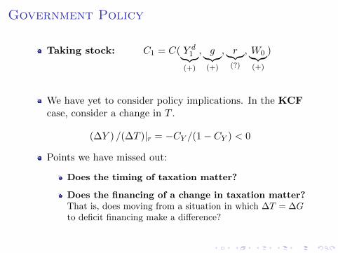
Government Policy
Taking stock: C1 = C( Y d1︸︷︷︸
(+)
, g︸︷︷︸(+)
, r︸︷︷︸(?)
, W0︸︷︷︸(+)
)
We have yet to consider policy implications. In the KCFcase, consider a change in T .
(∆Y ) /(∆T )|r = −CY /(1− CY ) < 0
Points we have missed out:
Does the timing of taxation matter?
Does the financing of a change in taxation matter?That is, does moving from a situation in which ∆T = ∆Gto deficit financing make a difference?
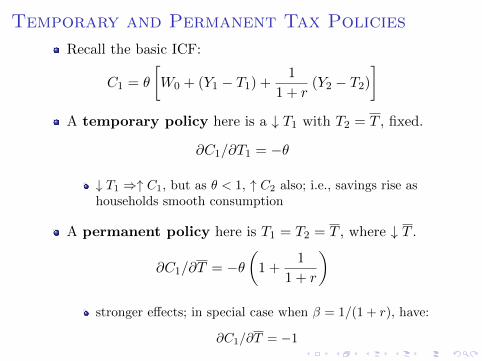
Temporary and Permanent Tax Policies
Recall the basic ICF:
C1 = θ
[W0 + (Y1 − T1) +
1
1 + r(Y2 − T2)
]A temporary policy here is a ↓ T1 with T2 = T , fixed.
∂C1/∂T1 = −θ
↓ T1 ⇒↑ C1, but as θ < 1, ↑ C2 also; i.e., savings rise ashouseholds smooth consumption
A permanent policy here is T1 = T2 = T , where ↓ T .
∂C1/∂T = −θ(
1 +1
1 + r
)stronger effects; in special case when β = 1/(1 + r), have:
∂C1/∂T = −1
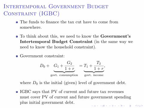
Intertemporal Government BudgetConstraint (IGBC)
The funds to finance the tax cut have to come fromsomewhere.
To think about this, we need to know the Government’sIntertemporal Budget Constraint (in the same way weneed to know the household constraint).
Government constraint:
D0 + G1 +G2
1 + r︸ ︷︷ ︸govt. consumption
= T1 +T2
1 + r︸ ︷︷ ︸govt. income
,
where D0 is the initial (given) level of government debt.
IGBC says that PV of current and future tax revenuesmust cover PV of current and future government spendingplus initial government debt.
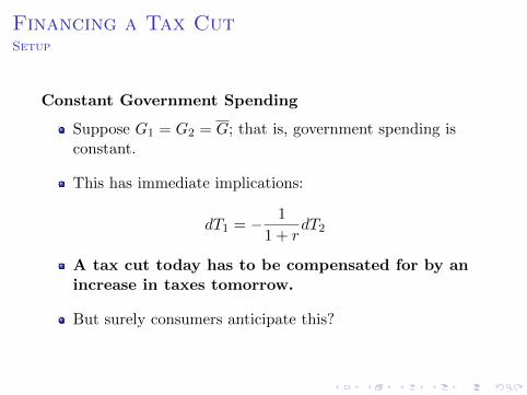
Financing a Tax CutSetup
Constant Government Spending
Suppose G1 = G2 = G; that is, government spending isconstant.
This has immediate implications:
dT1 = − 1
1 + rdT2
A tax cut today has to be compensated for by anincrease in taxes tomorrow.
But surely consumers anticipate this?
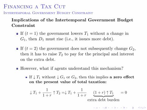
Financing a Tax CutIntertemporal Government Budget Constraint
Implications of the Intertemporal Government BudgetConstraint
If (t = 1) the government lowers T1 without a change inG1, then D1 must rise (i.e., it issues more debt).
If (t = 2) the government does not subsequently change G2,then it has to raise T2 to pay for the principal and intereston the extra debt.
However, what if agents understand this mechanism?
If ↓ T1 without ↓ G1 or G2, then this implies a zero effecton the present value of total taxation:
↓ T1 +1
1 + r↑ T2 =↓ T1 +
1
1 + r(1 + r) ↑ T1︸ ︷︷ ︸
extra debt burden
= 0
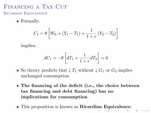
Financing a Tax CutRicardian Equivalence
Formally:
C1 = θ
[W0 + (Y1 − T1) +
1
1 + r(Y2 − T2)
]implies:
dC1 = −θ[dT1 +
1
1 + rdT2
]= 0
So theory predicts that ↓ T1 without ↓ G1 or G2 impliesunchanged consumption.
The financing of the deficit (i.e., the choice betweentax financing and debt financing) has noimplications for consumption.
This proposition is known as Ricardian Equivalence.

More on Ricardian Equivalence
Ricardian Equivalence should really be thought ofas a benchmark result. It breaks down if we change ourmodel only slightly; in particular:
Government and households have different planninghorizons.
However, Barro (1974) provides an interesting analysiswhen there are bequests between generations.
Intragenerational redistribution between heterogenousagents.
Distortionary taxation. (The taxes we have studied arelump-sum, i.e., there are no associated distortions. Underdistortionary taxation Ricardian Equivalence breaks down.)
Imperfect capital markets and credit constraints. (We don’ttend to borrow and lend at the same rate; some people are‘credit constrained’.)

Ricardian Equivalence - Empirical Evidence
Bernheim (1987), NBER Macro Annual
Keynesian view: deficit financed tax cut increasesaggregate demand
Ricardian view: taxpayers understand that PV of taxessimply depends on government spending; hence, tax cutswill have no effect on aggregate demand
Context: The mid 1980’s saw a high US governmentdeficit.
Main Finding: There is a short-run relationship betweendeficits and aggregate consumption both in cross-countrydata and in time-series tests of the consumption function.