Embed Size (px)
Citation preview
DOI: 10.1111/j.1475-679X.2010.00397.xJournal of Accounting Research
Vol. 00 No. 0 xxxx 2011Printed in U.S.A.
Earnings Quality Basedon Corporate Investment Decisions
F E N G L I ∗
Received 25 July 2007; accepted 20 September 2010
ABSTRACT
In this paper, I examine a new approach for measuring earnings quality, de-fined as the closeness of reported earnings to “permanent earnings,” based onfirm decisions with regard to capital and labor investments. Specifically, I mea-sure earnings quality as the contemporaneous association between changesin the levels of capital and labor investment and the change in reportedearnings. This approach follows the reasoning that (1) firms make invest-ment decisions based on the net present value (NPV) of investment projectsand (2) reported earnings with higher quality should more closely associatewith real investment decisions. I find that measures of earnings quality basedon managerial labor and capital decisions correlate positively with earningspersistence and have incremental explanatory power relative to earnings-quality measures used in the accounting literature. Furthermore, investment-based earnings-quality measures are less informative when managers tend tooverinvest.
1. Introduction
Prior research on earnings quality generally relies on one of two ap-proaches: studying the properties of accounting numbers or extracting
∗Stephen M. Ross School of Business, University of Michigan. I thank Ray Ball, Phil Berger,Ilia Dichev, Kenneth Merkley, workshop participants at the University of Chicago, and espe-cially an anonymous reviewer and Richard Leftwich (the journal editor) for their comments.
1
Copyright C©, University of Chicago on behalf of the Accounting Research Center, 2011
2 F. LI
information from stock prices.1 This paper explores a new measure of earn-ings quality by examining firm investment decisions.2 Managerial invest-ment decisions likely contain information about earnings quality becausemanagers make many decisions based on future profitability, and arguablyhave more precise and complete information about their firm’s profitabilitythan do other stakeholders. Therefore, to the extent that information asym-metry exists between managers and outsiders, the earnings quality inferredfrom managerial decisions can provide incremental information to existingempirical measures based on the information set of outside investors or onthe properties of the accounting numbers.3
In this study, I examine whether corporate investment decisions containinformation about earnings quality. In a simplified setting, managers in-vest more in projects with a higher net present value (NPV). All else be-ing equal, if a firm’s expected future earnings or permanent earnings in-crease, then it makes additional investment, because permanent earningsare equivalent to annuitized NPV (Black [1980], Beaver [1998], Ohlsonand Zhang [1998]). Hence, if a firm experiences an increase in reportedearnings and management views this earnings innovation to be permanent(i.e., the reported earnings have high “quality”), then that firm usually in-creases its investment level. However, if the innovation in reported earningsis purely transitory, then there should not be a corresponding change in theinvestment level. This reasoning suggests that earnings surprises that aremore associated with changes in corporate investment decisions are morelikely to be permanent and of higher quality than are earnings surprisesthat are less associated with such changes.
Inferring earnings quality from corporate investment decisions has lim-itations. Because of agency problems, managers have incentives to over-invest for empire building and other reasons (Stein [2003]). As a result,project profitability does not solely determine observed investment deci-sions and this reduces these decisions’ informativeness for assessing earn-ings quality. Ultimately, whether one can derive useful and reliable mea-sures of earnings quality from management investment decisions is anempirical question.
In this paper, I provide empirical evidence to answer this question byfirst examining whether corporate investment-based earnings-quality mea-sures are informative about future earnings. I measure earnings quality byexamining decisions regarding capital and labor investments, two of the
1 See, for instance, Sloan [1996], Dechow and Dichev [2002], Francis LaFond and Olsson[2005], Basu [1997], Collins Maydew and Weiss [1999], Francis and Schipper [1999], andEcker Francis and Kim [2006].
2 I define earnings quality as the closeness of reported earnings to the “permanent earn-ings” following Dechow and Schrand [2004] and use earnings persistence to operationalizethis concept.
3 Consistent with this argument, prior papers find that managerial decisions, which includedividend policy (Skinner and Soltes [2009]) and disclosure quality (Li [2008]), contain infor-mation about earnings quality.
EARNINGS QUALITY AND CORPORATE INVESTMENT 3
most important investment decisions managers make. I construct earnings-quality measures by regressing changes in the number of employees andthe amounts of capital and R&D expenditures on the change in reportedearnings, using rolling data from the last 10 years for every firm year. Theslopes from these regressions capture the sensitivity of investment to theinnovation in reported earnings and measure the information content ofthose earnings for expected future profitability as reflected in corporate in-vestment decisions. Because this regression approach requires a long timeseries of data, I also construct two other earnings-quality measures calcu-lated as the current changes in capital investment and labor investment (asproxied by the number of employees) divided by the change in reportedearnings for every firm year.
The empirical findings can be summarized as follows. First, the earnings-quality measures based on corporate investment decisions do not correlatehighly with other commonly used measures of earnings quality. This findingsuggests that the information contained in corporate investment decisionsdiffers somewhat from that reflected by stock prices and the properties ofhistorical accounting numbers. I then show that earnings-quality measuresbased on corporate investment decisions positively associate with earningspersistence. Furthermore, the predictive power of investment-based earn-ings quality for earnings persistence still holds and is economically mean-ingful even after controlling for typical measures of earnings quality suchas the absolute amount of accruals (Sloan [1996]), estimation errors inaccruals (Dechow and Dichev [2002]), the earnings–returns association,and the volatility of earnings and accruals. I also find that the investment-based earnings quality contains significant information about future earn-ings only for firms with a relatively low tendency to overinvest, measured us-ing the amount of free cash flows, the sensitivity of investment to cash flows,and the amount of excess investment based on Richardson [2006]. Finally, Ifind that the investment decisions are more informative about future earn-ings for capital-intensive firms, firms from highly unionized industries, andfirms with a high frequency of earnings increases. These additional testsfurther validate the utility of corporate investment decisions for assessingearnings quality.
Overall, the evidence indicates that there is substantial information incorporate investment decisions about earnings quality and it is incrementalto other commonly used earnings-quality measures. However, researchersor investors need to consider the severity of possible overinvestment dueto agency problems when using the investment-based earnings-quality mea-sures.
The remainder of this paper is organized as follows. Section 2 discussesthe literature on earnings quality and defines earnings-quality measuresbased on corporate investment decisions. Section 3 presents the data, sum-mary statistics of the measures, and their relation with firm characteristicsand other earnings-quality measures used in the literature. Section 4 pro-vides a discussion of the empirical results, and section 5 concludes.
4 F. LI
2. Literature and Hypotheses Development
2.1 LITERATURE ON EARNINGS QUALITY
There is an extensive literature on the earnings quality (see Dechowand Schrand [2004] for a comprehensive review). However, because of itscontext-dependent nature, there is no consensus on the underlying con-ceptual construct that “earnings quality” represents. In this paper, I followDechow and Schrand [2004] and define earnings quality as the closenessof reported earnings to the “permanent earnings” (Black [1980], Beaver[1998], and Ohlson and Zhang [1998]). I use earnings persistence to oper-ationalize this concept.
Earnings quality varies with many factors, including a firm’s businessmodel and economic situation, estimation errors (Dechow and Dichev[2002]), and earnings management (Healy and Wahlen [1999]). To cap-ture earnings quality, prior studies generally follow one of two approaches.The first approach measures earnings quality by using properties of the ob-served accounting numbers. The measures based on this approach includethe level of accruals (Sloan [1996]), the estimation error in accruals (De-chow and Dichev [2002]), and the volatility of earnings (Dichev and Tang[2009]). Because of the historical nature of the current accounting system,the information contained in accounting numbers is unlikely to be com-plete concerning future profitability. The second approach focuses on theassociation between earnings and stock returns (e.g., Basu [1997], CollinsMaydew and Weiss [1999], Francis and Schipper [1999], and Ecker Fran-cis and Kim [2006]). This approach assumes market efficiency and extractsinformation about future earnings from stock prices.
I take a different approach by emphasizing the management perspective.Managers arguably have more complete information about earnings qual-ity than do outsiders. Therefore, earnings-quality measures based on theinformation set of managers can provide better proxies for earnings qual-ity than measures that are based on historical accounting numbers or onthe information set of outside equity investors.
2.2 EARNINGS QUALITY BASED ON FIRM INVESTMENT DECISIONS
In a simplified setting, making corporate investment decisions is straight-forward: a firm invests more if the marginal NPV of the investment projectis positive. In accounting terms, the NPV of future investment is a mono-tonic function of the expected “permanent earnings,” which is essentiallythe annuitized NPV (Black [1980], Beaver [1998], and Ohlson and Zhang[1998]). Therefore, a firm invests (disinvests) if its permanent earningsincrease (decrease). Ignoring potential agency problems, the associationbetween firms’ observed investment decisions and reported earnings cap-tures the closeness of the reported earnings to the permanent earnings.Hence, the investment-earnings association provides information on thequality of the reported earnings. To the extent that managers have privateinformation that investors do not have, corporate investment decisions can
EARNINGS QUALITY AND CORPORATE INVESTMENT 5
provide informative signals about earnings quality relative to the market-based earnings-quality measures.
One point worth discussing is the parallel between a firm’s investmentdecision and the valuation of its equity by outside investors. In both cases,the involved parties (managers or investors) want to make their decisions bydoing valuations based on the expected profitability of the firm. Measuringearnings quality by using stock price information requires a maintained as-sumption of stock market efficiency, but assessing earnings quality throughmanagerial investment decisions relies on the assumption that managersmake optimal investment decisions.
I seek to contribute to the literature that explores the implications ofmanagerial decisions for earnings quality. Skinner and Soltes [2009] studythe information content of dividend decisions by firms for earnings qual-ity. Investment and dividend policies are both important managerial deci-sions and are likely to contain information about future earnings. Com-pared with dividend policy, firm labor and capital-investment decisions aresimpler in the sense that they are less likely to be influenced by signalingconsiderations. A subtle difference between this paper and Skinner andSoltes [2009] is that their emphasis is on testing the dividend informa-tion content hypothesis, which has been examined in the dividend liter-ature and has not received much support. The purpose of this paper is totest whether corporate investment decisions, despite potential agency prob-lems, can provide information about earnings quality that is incremental toother typical earnings-quality constructs. Consequently, it is important tocontrol for other measures of earnings quality.
Empirically, I examine two types of investment decisions and their asso-ciations with reported earnings: labor and capital investment. Labor andcapital are the two major factors that determine the output of a firm andthey are also the main managerial decision parameters in microeconomics.The labor- and capital-investment decisions can be affected by different eco-nomic factors. Therefore, examining both decisions can complement eachother.
2.3 OVERINVESTMENT AND INVESTMENT-BASED EARNINGS QUALITY
In this subsection, I explore the implications of firms’ nonoptimal invest-ment decision making for the investment-based earnings quality. My moti-vation is the existence of agency problems, a central theme in the corporatefinance literature with a lineage going back to Berle and Means [1932] andJensen and Meckling [1976]. Agency problems can lead to overinvestmentby managers (Stein [2003] provides a comprehensive review of the litera-ture). One consequence of the agency problem is that managers have anexcessive taste for running large firms, as opposed to simply profitable ones.This “empire building” tendency is emphasized by Williamson [1964], Don-aldson [1984], and Jensen [1986], among many other studies. Agencyproblems can also give rise to overinvestment through channels otherthan “empire building.” Bertrand and Mullainathan [2003] argue that amanagerial preference for the “quiet life”—effectively, a resistance to
6 F. LI
change—can lead to excessive continuation of negative-NPV projects. Ina somewhat similar vein, Baker [2000] builds a model in which reputa-tional concerns deter managers from discontinuing negative-NPV projects,because this would be an admission of failure.
Many empirical studies provide evidence on corporate overinvestment,including evidence from specific industries (e.g., the oil industry overin-vestment documented by Jensen [1986]) and evidence of poor acquisitions(Blanchard de Silanes and Shleifer [1994]). More recently, Richardson[2006] finds that investment decisions by firms are excessively sensitive tocurrent cash flows, which is a symptom of overinvestment.
Ceteris paribus, if a firm is more likely to overinvest, its labor- and capital-investment decisions are less likely to be a useful signal of earnings qualitybecause the investment decisions can be affected by other considerations(e.g., empire building motivations) and are not solely determined by theprofitability of the project. I therefore examine whether the informationcontent of the investment-based earnings-quality measures varies with theoverinvestment tendency cross-sectionally.
I use three empirical constructs to measure the overinvestment ten-dency. First, Richardson [2006] shows that firms with a large amount offree cash flows tend to overinvest. This finding implies that investment-based earnings-quality measures are less informative for firms with morefree cash flows. Second, a high sensitivity of investment to the free cashflows available for investment can indicate potential agency problems(Stein [2003]).4 Richardson [2006] also finds that firms that tend tooverinvest have higher investment–cash flow sensitivity. Hence, I use theinvestment–cash flow sensitivity as the second measure of the overinvest-ment tendency. Third, I rely directly on the overinvestment measure con-structed by Richardson [2006] for the cross-sectional tests. Because thismeasure directly relates to capital expenditure, I focus on the capitalinvestment-based earnings-quality measures.
To summarize, I expect that for firms that are likely to overinvest (i.e.,firms that have more free cash flows, higher sensitivity of investment tocash flows, and more excess investment), the investment-based measuresof earnings quality less strongly associate with earnings persistence and areless useful in predicting future earnings.
3. Estimation of Earnings Quality Based on Investment Decisions
3.1 EMPIRICAL ESTIMATION OF EARNINGS QUALITY
I obtain my sample from the Compustat annual industrial and researchfiles between 1952 and 2004. For every firm i in year T , I estimate the
4 The corporate finance literature also argues that firms with higher investment–cash flowsensitivity tend to have more severe financing constraints, in addition to overinvestment prob-lems. Nevertheless, the financial constraint interpretation of the investment–cash flow sensi-tivity also leads to a prediction of suboptimal investment for firms with higher investment–cashflow sensitivity.
EARNINGS QUALITY AND CORPORATE INVESTMENT 7
following two regressions using the data from year T − 9 to T :
(NEMPi,t − NEMPi,t−1)/TAi,t−1 = αL,iT + βL,iT (Ei,t − Ei,t−1)/TAi,t−1 + εL,i t
(1)and
(CAPX i,t + RNDi,t − CAPX i,t−1 − RNDi,t−1)/TAi,t−1
= αC,iT + βC,iT (Ei,t − Ei,t−1)/TAi,t−1 + εC,i t , (2)where T − 9 ≤ t ≤ T , NEMP is the number of employees at the end of a fis-cal year (#29 of the Compustat annual files), CAPX is the amount of capitalexpenditure for the year (#128), RND is the amount of R&D expenditurefor the year (#46), E is the operating earnings (#178) with some possibleadjustment (details in the next paragraph), and TA is the book value ofassets at the end of the fiscal year (#6).
Similar to prior studies (e.g., Richardson [2006]), I include R&D expen-diture in the capital investment together with capital expenditure. My mo-tivation is the fact that, even though R&D is fully expensed under currentU.S. generally accepted accounting principles (U.S. GAAP), prior studiesshow that the market views it more like an investment (Lev and Sougiannis[1996]). There is also a potential endogeneity problem in the estimationprocedure—an increase in capital and R&D expenditures in a given yearreduces the reported earnings because of additional expensing. This reduc-tion leads to a mechanical negative relation between investment and earn-ings. To mitigate this problem, I adjust the reported earnings by addingback the current R&D expense and the depreciation expense due to thenew capital expenditure. Specifically, for firm i in year t , Eit is calculated as
Eit = #178 + RNDit + CAPX it/(PPEit/DEPit ), (3)
where PPE is the average of the beginning and end values of the grossamount of property, plant, and equipment (#7) and DEP is the depreci-ation expense (#14). This adjustment assumes that the new assets, due tocurrent capital expenditure, are depreciated using the same rate as existingassets-in-place with a straight-line depreciation method.
Item #29 of Compustat represents the number of company workers (in-cluding all employees of consolidated domestic and foreign subsidiaries, allpart-time and seasonal employees, full-time equivalent employees, and offi-cers, and excluding consultants, contract workers, directors, and employeesof unconsolidated subsidiaries) as reported to shareholders.5 The amountof salary expense is a better variable to capture the amount of investment inlabor than the number of employees, especially when the scaling variableis the book value of assets. However, only about 20% of firm years in Com-pustat report a nonmissing labor expense (#42), but about 95% of the firm
5 This figure is reported by some firms as an average number of employees and by othersas the number of employees at year end. If both are given, the year-end figure is used. Thereis no reason to believe that this difference introduces a systematic bias to our estimates.
8 F. LI
years have the number of employees (#29). Using the number of employ-ees therefore can increase the number of observations dramatically. Thenumber of employees scaled by the book value of assets captures the laborintensity (i.e., the number of employees per dollar of assets). To the ex-tent that the salary per employee remains relatively stable over time for thesame firm, scaling the number of employees by total assets is not a problem.In unreported analysis, I also redo all the tests by replacing the dependentvariable in equation (1) with log(NEMPt/NEMPt−1) and the results are sim-ilar.
I use a firm-level regression because managerial decisions most natu-rally apply at the firm level. I expect that a firm-level specification is bet-ter than cross-sectional specifications because the regression coefficientsare likely to differ across firms because managers have firm-specific infor-mation about future profitability. The βL and βC are the “response coef-ficients” of corporate investment level to current reported earnings. For afirm to have βL and βC estimated in year t, it needs to have nonmissing datain the 10 years from t − 9 to t to estimate equations (1) and (2).
Because this regression approach uses 10 years of rolling data and there-fore shrinks the sample size greatly, I also construct two other measuresof earnings quality based on investment decisions for firm i in year T asfollows:
γL,iT = (NEMPiT − NEMPi,T−1)/(EiT − Ei,T−1) (4)
and
γC,iT = (CAPX iT + RNDiT − CAPX i,T−1 − RNDi,T−1)/(EiT − Ei,T−1), (5)
where all the definitions of the variables are the same as in equations (1)and (2). Thus, γ L and γ C capture the response of investment to the changein earnings in a given year. Compared with βL and βC , the advantage ofthese measures is that they require only two years of data, but the cost is thatthey might not measure the association between earnings and investmentprecisely and that it is more difficult to interpret the measures when thechange in earnings is negative.6
Also, I construct two measures that combine the information content ofboth the capital and labor investment decisions. To smooth out any possiblenonlinear effect of the variables, I average the measures based on capitaland labor decisions using their decile ranks
EQ 1 = (Decile(βL) + (Decile(βC ))/2 (6)
and
EQ 2 = (Decile(γL) + (Decile(γC ))/2, (7)
where Decile(·) is the decile rank of a variable in a year.
6 This is especially true during recession years.
EARNINGS QUALITY AND CORPORATE INVESTMENT 9
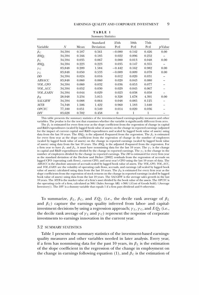
T A B L E 1Summary Statistics
Standard 25th 50th 75thVariable N Mean Deviation Pctl Pctl Pctl p-ValueβC 34,594 0.187 0.561 −0.080 0.142 0.426 0.00RSQC 34,594 0.166 0.185 0.022 0.096 0.252 –βL 34,594 0.035 0.067 0.000 0.013 0.048 0.00RSQL 34,594 0.223 0.223 0.035 0.147 0.355 –γ C 83,848 0.209 1.584 −0.442 0.162 0.982 0.00γ L 83,848 0.050 0.533 −0.009 0.009 0.078 0.00DD 34,594 0.024 0.016 0.012 0.020 0.031 –ABSACC 83,848 0.060 0.060 0.020 0.043 0.080 –VOL CFO 34,594 0.060 0.032 0.036 0.053 0.077 –VOL ACC 34,594 0.052 0.030 0.029 0.045 0.067 –VOL EARN 34,594 0.044 0.029 0.023 0.038 0.058 –βR 28,948 3.234 5.815 0.328 1.678 4.391 0.00SALGRW 34,594 0.088 0.064 0.048 0.085 0.125 –MTB 74,348 1.506 1.422 0.960 1.183 1.640 –OPCYC 77,100 0.051 0.549 0.014 0.020 0.036 –DIV 83,628 0.702 0.458 0 1 1 –
This table presents the summary statistics of the investment-based earnings-quality measures and othervariables. The p-value is for the test that examines whether the variable is significantly different from zero.
The βC is estimated for every firm year as the slope coefficient from the regression of change in capitaland R&D expenditures (scaled by lagged book value of assets) on the change in reported earnings (adjustedfor the impact of current capital and R&D expenditures and scaled by lagged book value of assets) usingdata from the last 10 years. The RSQ C is the adjusted R -squared from the regression. The βL is estimatedfor every firm year as the slope coefficient from the regression of change in the number of employees(scaled by lagged book value of assets) on the change in reported earnings (scaled by lagged book valueof assets) using data from the last 10 years. The RSQL is the adjusted R -squared from the regression. Fora firm year to have βC and βL , it must have nonmissing data for the last 10 years. The γ C is the changein capital and R&D expenditures divided by the change in reported earnings. The γ L is the change in thenumber of employees divided by the change in reported earnings. The DD is estimated for every firm yearas the standard deviation of the Dechow and Dichev [2002] residuals from the regression of accruals onlagged CFO (operating cash flows), current CFO, and next year’s CFO using the last 10 years of data. TheABSACC is the absolute amount of accruals scaled by lagged book value of assets. The VOL CFO, VOL ACC ,and VOL EARN are the volatility of operating cash flows, accruals, and earnings (all scaled by lagged bookvalue of assets) calculated using data from the last 10 years. The βR is estimated for every firm year as theslope coefficients from the regression of stock returns on the change in reported earnings (scaled by laggedbook value of assets) using data from the last 10 years. The SALGRW is the average sales growth in the last10 years. The MTB is the market value of a firm’s asset divided by the book value of the assets. The OPCYC isthe operating cycle of a firm, calculated as 360/(Sales Average AR) +360/((Cost of Goods Sold)/(AverageInventory)). The DIV is a dummy variable that equals 1 if a firm pays dividend and 0 otherwise.
To summarize, βL, βC , and E Q 1 (i.e., the decile rank average of βL
and βC ) capture the earnings quality inferred from labor- and capital-investment decisions by using a regression approach; γ L, γ C , and E Q 2 (i.e.,the decile rank average of γ L and γ C ) represent the response of corporateinvestments to earnings innovation in the current year.
3.2 SUMMARY STATISTICS
Table 1 presents the summary statistics of the investment-based earnings-quality measures and other variables needed in later analysis. Every year,if a firm has nonmissing data for the past 10 years, its βL is the estimationof the slope coefficient in the regression of the change in employment onthe change in earnings following equation (1), and βC is the estimation of
10 F. LI
the slope coefficient in the regression of the change in capital investmenton the change in earnings using equation (2). Because of the 10-year datarequirement, the sample size is relatively small (34,594 firm years or about800 firms per year).7
As predicted, current changes in reported earnings positively relate tothe contemporaneous changes in the level of labor and capital. As indi-cated in table 1, the mean coefficient on earnings change in the labor re-gression (βL) is 0.035 and the median is 0.013. The mean and median ofβC are 0.187 and 0.142, respectively. The RSQL and RSQC are the adjustedR -squared from the regressions that have a mean of 0.223 and 0.166, re-spectively, and indicate that earnings changes can explain 17–22% of thevariations in the changes of labor and capital investment. Based on thecross-sectional distribution of the coefficients, βL and βC are both statisti-cally significant with p-values of 0.00. The variations in the two measures aresubstantial: the standard deviations of βL and βC are 0.067 and 0.561 andtheir inter-quartile ranges are 0.048 and 0.506, respectively.
Table 1 also presents the summary statistics of γ L and γ C , the estimatesof earnings quality defined in equations (4) and (5). Because the estimatesonly require two years of data, the sample size is much bigger—83,848 firmyears (or about 2,000 firms per year). The γ L and γ C have a mean of 0.050and 0.209, respectively and both have substantial variations with standarddeviations of 0.533 and 1.584.
The table also presents the summary statistics of other commonly usedmeasures of earnings quality. The DD is the standard deviation of accrualsthat cannot be explained by cash flows as defined in Dechow and Dichev[2002], and is calculated using data from the last 10 years. The βR is theearnings–returns association calculated as the slope coefficient in the re-gression of stock returns on the change in reported earnings using datafrom the last 10 years. The ABSACC is the absolute amount of accrualsscaled by lagged book value of assets. The V OL CF O, V OL ACC , andV OL E ARN are the volatilities of cash flows, accruals, and earnings (allscaled by lagged book value of assets) calculated using data from the last 10years.
3.3 INVESTMENT-BASED EARNINGS QUALITY AND OTHER MEASURESOF EARNINGS QUALITY
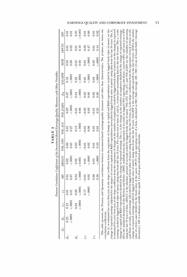
In this subsection, I examine the associations between the earnings-quality measures developed in this paper (i.e., βL, βC , γ L, and γ C ) and firmcharacteristics and other earnings-quality measures, such as the Dechowand Dichev [2002] measure, absolute value of accruals, volatility of earn-ings, earnings–returns association, growth, market-to-book ratio, and firmoperating cycle. Table 2 presents the Pearson correlation coefficients be-tween the investment-based earnings-quality measures and these variables.
7 To remove the influence of extreme observations, all variables are winsorized at the 1%and 99% levels.
EARNINGS QUALITY AND CORPORATE INVESTMENT 11
TA
BL
E2
Pear
son
Cor
rela
tion
Coe
ffici
ents
ofth
eIn
vest
men
t-Bas
edEa
rnin
gs-Q
ualit
yM
easu
res
with
Oth
erVa
riab
les
βC
βL
γC
γL
DD
AB
SAC
CVO
LC
FOVO
LA
CC
VOL
EAR
Nβ
RSA
LG
RW
MT
BO
PCYC
DIV
βC
0.23
0.12
0.01
0.01
0.02
0.00
0.01
0.03
0.07
0.16
0.03
0.01
0.01
<.0
001
<.0
001
0.01
0.87
<.0
001
0.65
0.27
<.0
001
<.0
001
<.0
001
0.00
0.02
0.01
βL
0.04
0.08
0.04
0.02
0.03
0.13
−0.0
10.
040.
22−0
.01
0.01
0.05
<.0
001
<.0
001
<.0
001
<0.
001
<.0
001
<.0
001
0.06
<.0
001
<.0
001
0.02
0.10
<0.
001
γC
0.17
−0.0
10.
03−0
.01
−0.0
1−0
.02
0.02
0.05
0.04
0.00
0.01
<.0
001
0.02
<.0
001
0.02
0.06
0.02
0.00
<.0
001
<.0
001
0.47
0.00
γL
0.00
0.03
0.01
0.01
−0.0
10.
020.
040.
020.
010.
010.
58<
.000
10.
100.
010.
250.
00<
.000
1<
.000
10.
140.
02T
his
tabl
epr
esen
tsth
ePe
arso
nan
dSp
earm
anco
rrel
atio
nsbe
twee
nin
vest
men
t-bas
edea
rnin
gs-q
ualit
ym
easu
res
and
othe
rfir
mch
arac
teri
stic
s.T
hep-
valu
esar
ebe
low
the
corr
elat
ion
coef
ficie
nts.
The
βC
ises
timat
edfo
rev
ery
firm
year
asth
esl
ope
coef
ficie
ntfr
omth
ere
gres
sion
ofch
ange
inca
pita
land
R&
Dex
pend
iture
s(s
cale
dby
lagg
edbo
okva
lue
ofas
sets
)on
the
chan
gein
repo
rted
earn
ings
(adj
uste
dfo
rth
eim
pact
ofcu
rren
tcap
itala
ndR
&D
expe
nditu
res
and
scal
edby
lagg
edbo
okva
lue
ofas
sets
)us
ing
data
from
the
last
10ye
ars.
The
βL
ises
timat
edfo
rev
ery
firm
year
asth
esl
ope
coef
ficie
ntfr
omth
ere
gres
sion
ofch
ange
inth
enu
mbe
rof
empl
oyee
s(s
cale
dby
lagg
edbo
okva
lue
ofas
sets
)on
the
chan
gein
repo
rted
earn
ings
(sca
led
byla
gged
book
valu
eof
asse
ts)
usin
gda
tafr
omth
ela
st10
year
s.Fo
ra
firm
year
toha
veβ
Can
dβ
L,i
tmus
thav
eno
nmis
sing
data
for
the
last
10ye
ars.
The
γC
isth
ech
ange
inca
pita
land
R&
Dex
pend
iture
sdi
vide
dby
the
chan
gein
repo
rted
earn
ings
.The
γL
isth
ech
ange
inth
enu
mbe
rof
empl
oyee
sdi
vide
dby
the
chan
gein
repo
rted
earn
ings
.D
Dis
the
stan
dard
devi
atio
nof
the
Dec
how
and
Dic
hev
[200
2]re
sidu
als
from
the
regr
essi
onof
accr
uals
onla
gged
CFO
(ope
ratin
gca
shfl
ows)
,cur
rent
CFO
,and
next
year
’sC
FOus
ing
the
last
10ye
ars
ofda
ta.A
BSA
CC
isth
eab
solu
team
ount
ofac
crua
lssc
aled
byla
gged
book
valu
eof
asse
ts.V
OL
CFO
,VO
LA
CC
,and
VOL
EAR
Nar
eth
evo
latil
ityof
oper
atin
gca
shfl
ows,
accr
uals
,and
earn
ings
(all
scal
edby
lagg
edbo
okva
lue
ofas
sets
)us
ing
data
from
the
last
10ye
ars.
βR
isth
esl
ope
coef
ficie
nts
from
the
regr
essi
onof
stoc
kre
turn
son
the
chan
gein
repo
rted
earn
ings
(sca
led
byla
gged
book
valu
eof
asse
ts)
usin
gda
tafr
omth
ela
st10
year
s.SA
LG
RW
isth
eav
erag
esa
les
grow
thin
the
last
10ye
ars.
MT
Bis
the
mar
ket
valu
eof
afir
m’s
asse
tdi
vide
dby
the
book
valu
eof
the
asse
ts.O
PCYC
isth
eop
erat
ing
cycl
eof
afir
m,c
alcu
late
das
360/
(Sal
esA
vera
geA
R)
+360
/((C
ost
ofG
oods
Sold
)/(A
vera
geIn
vent
ory)
).D
IVis
adu
mm
yva
riab
leth
ateq
uals
1if
afir
mpa
ysdi
vide
ndan
d0
othe
rwis
e.
12 F. LI
Table 2 shows a correlation between βL and βC with a Pearson correlationcoefficient of 0.23 (p-value < 0.001); similarly, the Pearson correlation co-efficient between γ L and γ C is 0.17 (p-value< 0.001). This finding suggeststhat labor- and capital-investment decisions capture common informationin earnings.
The evidence in table 2 also shows that the earnings-quality measuresdeveloped from corporate investment decisions do not have a strong cor-relation with other common measures of earnings quality. For instance, DD(the standard deviation of accruals that cannot be explained by CF Ot−1,CF Ot , and CF Ot+1 based on Dechow and Dichev [2002]) has a Pearsoncorrelation of 0.01 (p-value = 0.87) with βC , 0.04 (p-value < 0.001) with βL,−0.01 (p-value = 0.02) with γ C , and 0.00 (p-value = 0.58) with γ L. Theseresults show that DD captures a different set of information from that ofthe investment-based earnings-quality measures. Sales growth is the variablewith the largest correlation with the investment-based earnings-quality mea-sures: firms with a high sales growth rate tend to have stronger associationsbetween earnings and investment. For instance, βL has a Pearson correla-tion of 0.22 (p< 0.001) with the 10-year sales growth rate (SALGRW ).
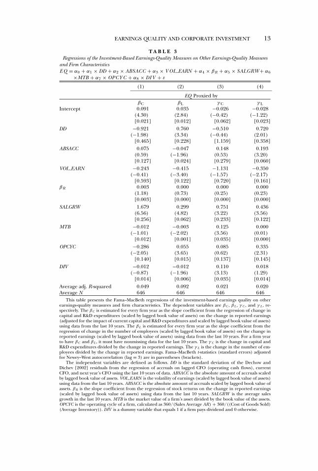
In table 3, I examine the relation between βC , βL, γ C , and γ L and otherearnings-quality measures and firm characteristics using a Fama–MacBethregression approach. Every year, I regress the investment-based earnings-quality measures on other variables, and the table reports the means andt-statistics based on the time-series distribution of the coefficients. Sincethe data that estimates βC and βL is the rolling data from the last 10 years,there are serial correlations in the error terms when they are the dependentvariables. To mitigate this concern, I adjust the Fama–MacBeth t-statisticsfor serial correlations using the Newey–West procedure with a lag of three.8
Consistent with the univariate correlations reported in table 2, thereseems to be no robust relation between the investment-based earnings-quality measures and many of the commonly used earnings-quality vari-ables. For instance, DD, the standard deviation of the accruals residualsbased on Dechow and Dichev [2002], is negatively associated with βC (co-efficient on DD = −0.921 and t = −1.98), but is positively related to βL (co-efficient 0.760 and t = 3.34). As another example, although the volatility ofearnings is consistently negatively associated with the earnings-quality mea-sures based on corporate investment, it is statistically significant only forβL and γ L. The only robust and significant factor that explains βC , βL, γ C ,and γ L is SALGRW , the 10-year sales growth rate, which is positively andsignificantly associated with all four variables.
Overall, the correlations between the investment-based earnings-qualitymeasures and other typical measures of earnings quality are modest, whichsuggests that corporate investment decisions capture information about
8 Newey and West [1994] suggest that the optimal length for the Newey–West adjustment isT 1/4, where T is the time-series length of the data.
EARNINGS QUALITY AND CORPORATE INVESTMENT 13
T A B L E 3Regressions of the Investment-Based Earnings-Quality Measures on Other Earnings-Quality Measures
and Firm CharacteristicsE Q = α0 + α1 × DD + α2 × ABSACC + α3 × V OL EARN + α4 × βR + α5 × SALGRW + α6
×MTB + α7 × OPCY C + α8 × DI V + ε
(1) (2) (3) (4)
EQ Proxied byβC βL γ C γ L
Intercept 0.091 0.035 −0.026 −0.028(4.30) (2.84) (−0.42) (−1.22)[0.021] [0.012] [0.062] [0.023]
DD −0.921 0.760 −0.510 0.720(−1.98) (3.34) (−0.44) (2.01)
[0.465] [0.228] [1.159] [0.358]ABSACC 0.075 −0.047 0.148 0.193
(0.59) (−1.96) (0.53) (3.20)[0.127] [0.024] [0.279] [0.060]
VOL EARN −0.243 −0.415 −1.131 −0.350(−0.41) (−3.40) (−1.57) (−2.17)
[0.593] [0.122] [0.720] [0.161]βR 0.003 0.000 0.000 0.000
(1.18) (0.73) (0.25) (0.23)[0.003] [0.000] [0.000] [0.000]
SALGRW 1.679 0.299 0.751 0.436(6.56) (4.82) (3.22) (3.56)[0.256] [0.062] [0.233] [0.122]
MTB −0.012 −0.003 0.125 0.000(−1.01) (−2.02) (3.56) (0.01)
[0.012] [0.001] [0.035] [0.000]OPCYC −0.286 0.055 0.085 0.335
(−2.05) (3.65) (0.62) (2.31)[0.140] [0.015] [0.137] [0.145]
DIV −0.012 −0.012 0.110 0.018(−0.87) (−1.96) (3.13) (1.29)
[0.014] [0.006] [0.035] [0.014]Average adj. R -squared 0.049 0.092 0.021 0.020Average N 646 646 646 646
This table presents the Fama–MacBeth regressions of the investment-based earnings quality on otherearnings-quality measures and firm characteristics. The dependent variables are βC , βL , γ C , and γ L , re-spectively. The βC is estimated for every firm year as the slope coefficient from the regression of change incapital and R&D expenditures (scaled by lagged book value of assets) on the change in reported earnings(adjusted for the impact of current capital and R&D expenditures and scaled by lagged book value of assets)using data from the last 10 years. The βL is estimated for every firm year as the slope coefficient from theregression of change in the number of employees (scaled by lagged book value of assets) on the change inreported earnings (scaled by lagged book value of assets) using data from the last 10 years. For a firm yearto have βC and βL , it must have nonmissing data for the last 10 years. The γ C is the change in capital andR&D expenditures divided by the change in reported earnings. The γ L is the change in the number of em-ployees divided by the change in reported earnings. Fama–MacBeth t-statistics (standard errors) adjustedfor Newey–West autocorrelation (lag = 3) are in parentheses (brackets).
The independent variables are defined as follows. DD is the standard deviation of the Dechow andDichev [2002] residuals from the regression of accruals on lagged CFO (operating cash flows), currentCFO, and next year’s CFO using the last 10 years of data. ABSACC is the absolute amount of accruals scaledby lagged book value of assets. VOL EARN is the volatility of earnings (scaled by lagged book value of assets)using data from the last 10 years. ABSACC is the absolute amount of accruals scaled by lagged book value ofassets. βR is the slope coefficient from the regression of stock returns on the change in reported earnings(scaled by lagged book value of assets) using data from the last 10 years. SALGRW is the average salesgrowth in the last 10 years. MTB is the market value of a firm’s asset divided by the book value of the assets.OPCYC is the operating cycle of a firm, calculated as 360/(Sales Average AR) + 360/((Cost of Goods Sold)(Average Inventory)). DIV is a dummy variable that equals 1 if a firm pays dividend and 0 otherwise.
14 F. LI
future earnings that is somewhat different from that reflected in the othervariables.
4. Empirical Results
4.1 INVESTMENT-BASED EARNINGS QUALITY AND EARNINGS PERSISTENCE
In this subsection, I present evidence that the earnings-quality measuresbased on firm labor and capital changes are informative about earningspersistence. To test this prediction, I estimate the following regression:
(Ei,t+1/TAi,t−1) = α0 + α1(Eit/TAi,t−1) + α2EQ it + α3EQ it(Eit/TAi,t−1)
+α4CONTROLit + α5CONTROLit(Eit/TAi,t−1) + εit ,
(8)
where Eit is earnings for firm i in year t , TAit is total assets for firm i inyear t, and E Qit is the earnings-quality measure of firm i in year t. If βL, βC ,or E Q 1 (the decile rank average of βL and βC ) proxies for E Qit , then theearnings-quality estimation requires data for firm i from year t − 9 to t; ifγ L, γ C , or E Q 2 (the decile rank average of γ L and γ C ) proxies for it, thenthe calculation uses data from year t and t − 1. In this regression, α2 mea-sures the persistence of earnings. Under the hypothesis that investment de-cisions are informative about the quality of reported earnings, I expect thecoefficient on current earnings to be larger for firms with a higher associa-tion between investment and earnings, which indicates that their earningsare more persistent (α3 > 0).
To assess the incremental information content of the investment-basedearnings-quality measures, the regression includes typical measures of earn-ings quality and their interactions with Eit . In the reported results, I use thefollowing control variables: earnings–returns association (βR), the absoluteamount of accruals in current earnings (ABSACC), the Dechow and Dichev[2002] measure of accruals quality (DD), and a dummy variable for currentdividend (DIV ) that equals one if a firm issues dividend and zero otherwise.In untabulated results, I further control for the volatility of earnings, thevolatility of cash flows, the market-to-book ratio, and the e-loadings mea-sure proposed by Ecker, Francis, and Kim [2006], because these variablesare also used as measures of earnings quality in the literature. These untab-ulated results remain qualitatively similar to the reported results.9 All of theregressions use the Fama and MacBeth [1973] approach with Newey–Westadjustment to standard errors.
Panel A of table 4 reports the results of estimating equation (8) with EQproxied by βL, βC , and their decile rank average (E Q 1). For my sample, the
9 I do not report the results with all the control variables because many of the variables arehighly correlated with each other. For instance, accruals volatility is highly correlated with theDechow and Dichev [2002] measure; including both variables in the regression makes it hardto interpret the coefficients.
EARNINGS QUALITY AND CORPORATE INVESTMENT 15
TA
BL
E4
Pers
iste
nce
asa
Func
tion
ofth
eIn
vest
men
t-Bas
edEa
rnin
gs-Q
ualit
yM
easu
res
(Eit+1
/TA
it−1
)=
α0
+α
1×(
Eit
/TA
it−1
)+α
2×
EQ
it+
α3
×E
Qit
×(E
it/T
Ait−1
)+
α4
×C
ON
TR
OL
it+
α5
×C
ON
TR
OL
it×(
Eit
/TA
it−1
)+
εit
Pan
elA
:Ear
ning
sQ
ualit
yM
easu
red
byU
sing
the
Reg
ress
ion
App
roac
h(1
)(2
)(3
)(4
)(5
)(6
)(7
)(8
)(9
)EQ
Prox
ied
by
βC
βL
βC
βL
βC
βL
EQ1
EQ1
Inte
rcep
t(α
0)0.
010
0.01
00.
011
0.01
70.
018
0.01
00.
011
0.01
50.
015
(5.5
5)(5
.60)
(4.7
0)(5
.06)
(4.8
2)(3
.02)
(3.0
7)(5
.95)
(3.8
2)[0
.002
][0
.002
][0
.002
][0
.003
][0
.004
][0
.003
][0
.004
][0
.003
][0
.004
]E
(α1)
1.02
71.
003
1.00
30.
870
0.86
70.
953
0.95
10.
951
0.90
6(7
9.17
)(9
0.27
)(7
8.19
)(2
5.39
)(2
4.45
)(2
8.27
)(2
6.65
)(1
06.0
4)(2
4.53
)[0
.013
][0
.011
][0
.013
][0
.034
][0
.035
][0
.034
][0
.036
][0
.009
][0
.037
]EQ
(α2)
−0.0
06−0
.046
−0.0
04−0
.042
−0.0
03−0
.053
−0.0
01−0
.001
(−3.
50)
(−4.
16)
(−2.
88)
(−5.
63)
(−2.
33)
(−4.
17)
(−2.
94)
(−3.
32)
[0.0
02]
[0.0
11]
[0.0
01]
[0.0
07]
[0.0
01]
[0.0
13]
[0.0
00]
[0.0
00]
EQ
×E
(α3)
0.06
40.
446
0.04
10.
377
0.03
80.
442
0.01
20.
011
(5.0
6)(7
.97)
(3.6
6)(7
.17)
(3.2
8)(4
.89)
(4.9
1)(4
.65)
[0.0
13]
[0.0
56]
[0.0
11]
[0.0
53]
[0.0
12]
[0.0
90]
[0.0
02]
[0.0
02]
βR
(α4,
1)−0
.001
−0.0
01−0
.001
−0.0
01−0
.001
(−3.
88)
(−3.
69)
(−3.
90)
(−3.
64)
(−3.
68)
[0.0
00]
[0.0
00]
[0.0
00]
[0.0
00]
[0.0
00]
βR
×E
(α5,
1)0.
006
0.00
60.
006
0.00
60.
006
(5.6
2)(5
.70)
(5.5
2)(5
.42)
(5.4
0)[0
.001
][0
.001
][0
.001
][0
.001
][0
.001
](C
ontin
ued)
16 F. LI
TA
BL
E4
—C
ontin
ued
Pan
elA
:Ear
ning
sQ
ualit
yM
easu
red
byU
sing
the
Reg
ress
ion
App
roac
h(1
)(2
)(3
)(4
)(5
)(6
)(7
)(8
)(9
)EQ
Prox
ied
by
βC
βL
βC
βL
βC
βL
EQ1
EQ1
AB
SAC
C(α
4,2)
0.07
40.
074
(3.0
2)(3
.02)
[0.0
25]
[0.0
25]
AB
SAC
C×
E(α
5,2)
−0.0
86−0
.099
(−0.
55)
(−0.
63)
[0.1
56]
[0.1
57]
DD
(α4,
3)
0.32
60.
340
0.33
8(4
.48)
(4.3
4)(4
.30)
[0.0
73]
[0.0
78]
[0.0
79]
DD
×E
(α5,
3)
−2.2
71−2
.361
−2.4
28(−
3.64
)(−
3.68
)(−
3.73
)[0
.624
][0
.642
][0
.651
]D
IV(α
4,4)
−0.0
10−0
.010
−0.0
08−0
.008
−0.0
08(−
4.38
)(−
4.24
)(−
3.42
)(−
3.23
)(−
3.32
)[0
.002
][0
.002
][0
.002
][0
.002
][0
.002
]D
IV×
E(α
5,4)
0.13
50.
133
0.10
60.
103
0.10
5(3
.91)
(3.8
8)(3
.35)
(3.2
1)(3
.26)
[0.0
35]
[0.0
34]
[0.0
32]
[0.0
32]
[0.0
32]
Ave
rage
adj.
R-sq
uare
d0.
695
0.74
00.
740
0.75
60.
756
0.75
70.
758
0.74
10.
758
Ave
rage
N1,
610
820
820
679
679
679
679
820
679
No.
ofye
ars
5242
4242
4242
4242
42(C
ontin
ued)
EARNINGS QUALITY AND CORPORATE INVESTMENT 17
TA
BL
E4
—C
ontin
ued
Pan
elB
:Ear
ning
sQ
ualit
yM
easu
red
byU
sing
the
Non
regr
essi
onA
ppro
ach
(1)
(2)
(3)
(4)
(5)
(6)
(7)
(8)
EQPr
oxie
dby
γC
γL
γC
γL
γC
γL
EQ2
EQ2
Inte
rcep
t(α
0)0.
010
0.01
00.
010
0.01
00.
009
0.00
90.
019
0.01
2(5
.16)
(5.7
6)(3
.71)
(3.7
5)(2
.84)
(2.8
2)(7
.72)
(3.6
8)[0
.002
][0
.002
][0
.003
][0
.003
][0
.003
][0
.003
][0
.002
][0
.003
]E
(α1)
1.02
31.
022
1.03
51.
037
0.96
30.
961
0.88
80.
890
(79.
25)
(80.
18)
(31.
42)
(32.
82)
(29.
35)
(28.
77)
(51.
39)
(25.
37)
[0.0
13]
[0.0
13]
[0.0
33]
[0.0
32]
[0.0
33]
[0.0
33]
[0.0
17]
[0.0
35]
EQ(α
2)−0
.000
−0.0
05−0
.000
−0.0
040.
001
−0.0
03−0
.001
−0.0
01(−
1.16
)(−
4.35
)(−
0.99
)(−
3.95
)(0
.19)
(−1.
61)
(−5.
67)
(−1.
32)
[0.0
00]
[0.0
01]
[0.0
00]
[0.0
01]
[0.0
05]
[0.0
02]
[0.0
00]
[0.0
01]
EQ
×E
(α3)
0.01
10.
060
0.01
00.
054
0.00
40.
030
0.02
30.
012
(3.1
2)(5
.67)
(2.9
4)(5
.02)
(1.0
5)(2
.39)
(11.
72)
(5.0
0)[0
.004
][0
.011
][0
.003
][0
.011
][0
.004
][0
.013
][0
.002
][0
.002
]β
R(α
4,1)
−0.0
01−0
.001
−0.0
01(−
3.74
)(−
3.60
)(−
3.58
)[0
.000
][0
.000
][0
.000
]β
R×
E(α
5,1)
0.00
60.
006
0.00
6(5
.61)
(5.4
2)(5
.60)
[0.0
01]
[0.0
01]
[0.0
01]
AB
SAC
C(α
4,2)
0.07
80.
078
(5.3
3)(5
.28)
[0.0
15]
[0.0
15]
AB
SAC
C×
E(α
5,2)
−0.2
34−0
.238
(−2.
45)
(−2.
44)
[0.0
96]
[0.0
98]
(Con
tinue
d)
18 F. LI
TA
BL
E4
—C
ontin
ued
Pan
elB
:Ear
ning
sQ
ualit
yM
easu
red
byU
sing
the
Non
regr
essi
onA
ppro
ach
(1)
(2)
(3)
(4)
(5)
(6)
(7)
(8)
EQPr
oxie
dby
γC
γL
γC
γL
γC
γL
EQ2
EQ2
DD
(α4,
3)
0.33
10.
327
0.32
4(4
.64)
(4.5
4)(4
.50)
[0.0
71]
[0.0
72]
[0.0
72]
DD
×E
(α5,
3)
−2.2
33−2
.287
−2.2
61(−
3.86
)(−
3.78
)(−
3.79
)[0
.578
][0
.605
][0
.597
]D
IV(α
4,4)
−0.0
08−0
.007
−0.0
08−0
.008
−0.0
08(−
4.59
)(−
4.38
)(−
3.38
)(−
3.37
)(−
3.47
)[0
.002
][0
.002
][0
.002
][0
.002
][0
.002
]D
IV×
E(α
5,4)
0.02
00.
017
0.10
50.
107
0.10
5(0
.65)
(0.5
6)(3
.35)
(3.3
6)(3
.42)
[0.0
31]
[0.0
30]
[0.0
31]
[0.0
32]
[0.0
31]
Ave
rage
adj.
R-sq
uare
d0.
697
0.69
60.
704
0.70
30.
757
0.75
80.
699
0.75
9A
vera
geN
1,59
31,
610
1,58
91,
610
678
679
1,61
067
9N
o.of
year
s52
5252
5242
4252
42T
his
tabl
epr
esen
tsth
eFa
ma–
Mac
Bet
hre
gres
sion
sth
ates
timat
eea
rnin
gspe
rsis
tenc
eas
afu
nctio
nof
the
inve
stm
ent-b
ased
earn
ings
qual
ity.
The
depe
nden
tva
riab
leis
Eit+1
/TA
it−1
,ne
xtye
ar’s
earn
ings
scal
edby
the
lagg
edbo
okva
lue
ofas
sets
.Fa
ma–
Mac
Bet
ht-s
tatis
tics
(sta
ndar
der
rors
)ad
just
edfo
rN
ewey
–Wes
tau
toco
rrel
atio
n(l
ag=
3)ar
ein
pare
nthe
ses
(bra
cket
s).
The
inde
pend
entv
aria
bles
are
defin
edas
follo
ws.
Eis
,Eit
/TA
it−1
,cur
rent
earn
ings
scal
edby
the
lagg
edbo
okva
lue
ofas
sets
.The
βC
ises
timat
edfo
rev
ery
firm
year
asth
esl
ope
coef
ficie
ntfr
omth
ere
gres
sion
ofch
ange
inca
pita
land
R&
Dex
pend
iture
s(s
cale
dby
lagg
edbo
okva
lue
ofas
sets
)on
the
chan
gein
repo
rted
earn
ings
(adj
uste
dfo
rth
eim
pact
ofcu
rren
tca
pita
land
R&
Dex
pend
iture
san
dsc
aled
byla
gged
book
valu
eof
asse
ts)
usin
gda
tafr
omth
ela
st10
year
s.T
heβ
Lis
estim
ated
for
ever
yfir
mye
aras
the
slop
eco
effic
ient
from
the
regr
essi
onof
chan
gein
the
num
ber
ofem
ploy
ees
(sca
led
byla
gged
book
valu
eof
asse
ts)
onth
ech
ange
inre
port
edea
rnin
gs(s
cale
dby
lagg
edbo
okva
lue
ofas
sets
)us
ing
data
from
the
last
10ye
ars.
For
afir
mye
arto
have
βC
and
βL
,itm
usth
ave
nonm
issi
ngda
tafo
rth
ela
st10
year
s.EQ
1is
the
aver
age
ofth
ede
cile
rank
sof
βC
and
βL
.The
γC
isth
ech
ange
inca
pita
lexp
endi
ture
divi
ded
byth
ech
ange
inre
port
edea
rnin
gs.T
heγ
Lis
the
chan
gein
the
num
ber
ofem
ploy
ees
divi
ded
byth
ech
ange
inre
port
edea
rnin
gs.E
Q2
isth
eav
erag
eof
the
deci
lera
nks
ofγ
Can
dγ
L.D
Dis
the
stan
dard
devi
atio
nof
the
Dec
how
and
Dic
hev
[200
2]re
sidu
als
from
the
regr
essi
onof
accr
uals
onla
gged
CFO
(ope
ratin
gca
shfl
ows)
,cur
rent
CFO
,and
next
year
’sC
FOus
ing
the
last
10ye
ars
ofda
ta.A
BSA
CC
isth
eab
solu
team
ount
ofac
crua
ls,s
cale
dby
the
lagg
edbo
okva
lue
ofas
sets
.βR
isth
esl
ope
coef
ficie
ntfr
omth
ere
gres
sion
ofst
ock
retu
rns
onth
ech
ange
inre
port
edea
rnin
gs(s
cale
dby
lagg
edbo
okva
lue
ofas
sets
)us
ing
data
from
the
last
10ye
ars.
DIV
isa
dum
my
vari
able
that
equa
ls1
ifa
firm
pays
divi
dend
and
0ot
herw
ise.
EARNINGS QUALITY AND CORPORATE INVESTMENT 19
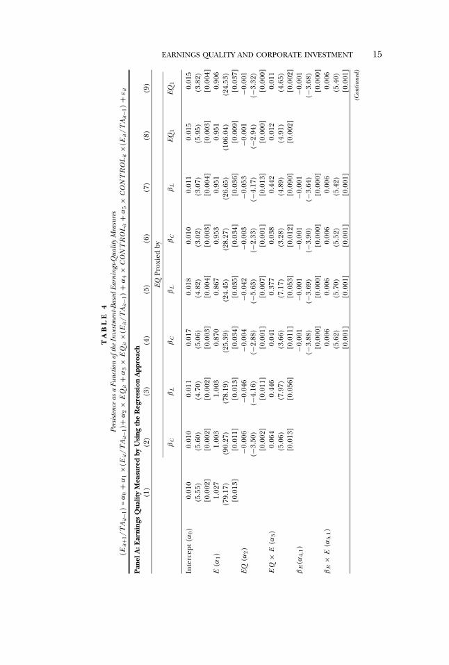
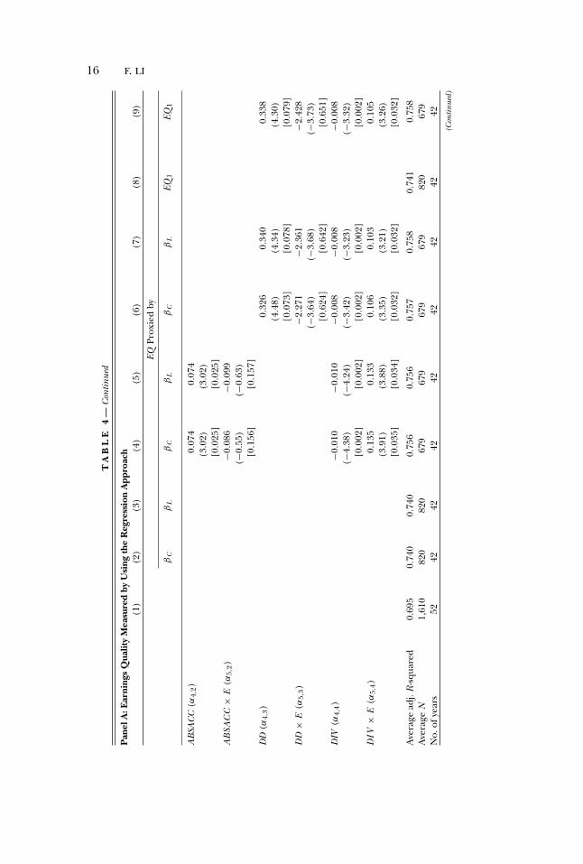
coefficient on earnings, when used alone to explain next year’s earnings,is 1.027 (column (1)). Consistent with the prediction, the coefficient onthe interaction of EQ and Eit is reliably positive, implying that earnings aremore persistent for firms with a higher association between investment andreported earnings. For instance, in column (2), the α3 is 0.064 (t = 5.06).The R -squared in column (2) is 0.74 and the R -squared in column (1) is0.70, which suggests that adding βC incrementally explains 4% more of thevariation in next year’s earnings.
When I control for the earnings–returns association, the absoluteamount of accruals, the Dechow–Dichev measure, and the dividenddummy, then the size of the α3 coefficient is smaller, but it remains eco-nomically and statistically significant. For example, in column (6), the co-efficient on the interaction of βC and Eit is 0.038 (t = 3.28). This effect isalso robust to using the rank specification of the earnings-quality measures.In column (9), when E Q 1 represents investment-based earnings quality,then the α3 is estimated at 0.011 (t = 4.65). This result implies a sub-stantial economic magnitude—increasing E Q 1 from decile 1 to decile 10means that earnings persistence increases by about 0.10. As a benchmark,the results in table 4 show that, after controlling for other variables, mov-ing DD from the bottom decile (i.e., 5th percentile = 0.006) to the topdecile (i.e., 95th percentile = 0.055) reduces the earnings persistence by0.11 (=(0.055−0.006)×(−2.3)).
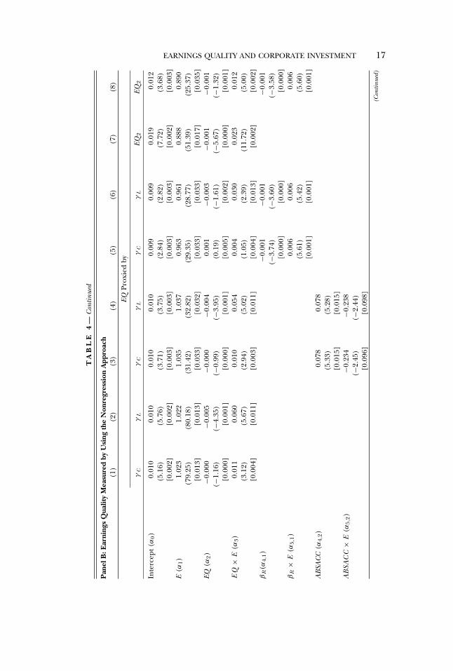
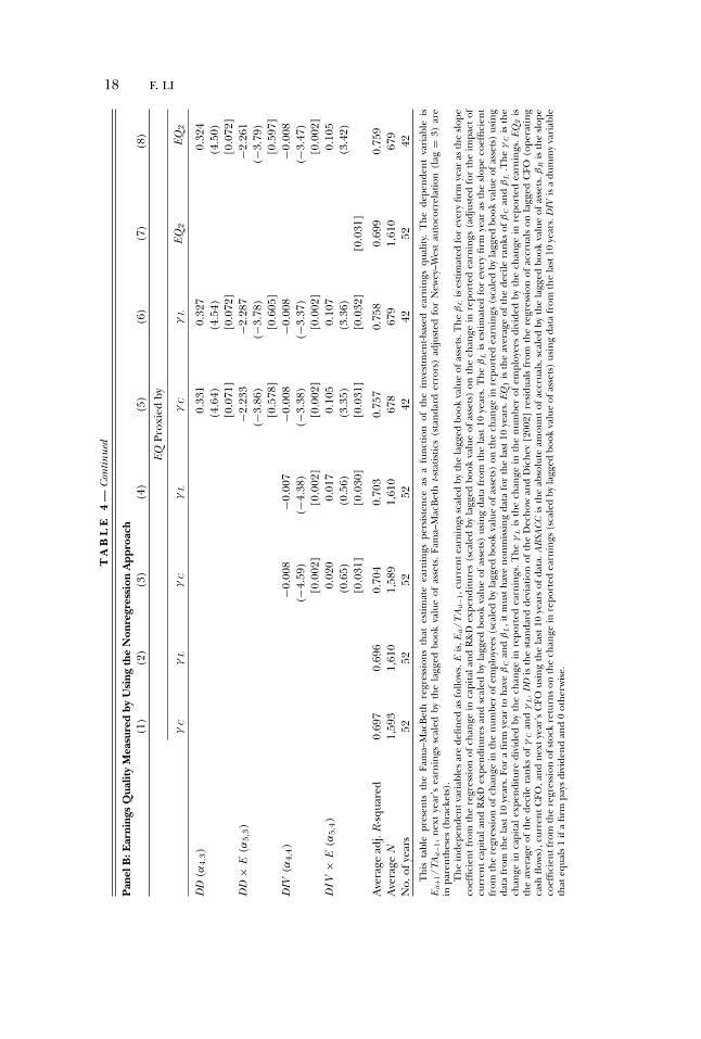
Panel B of table 4 presents the evidence based on γ L and γ C . The resultspaint the same picture as those from panel A. Throughout different spec-ifications, the interaction terms of the investment-based earnings-qualitymeasure and current earnings appear positive and statistically significant,with only the exception of column (5), where α3 is 0.004 and insignificant(t = 1.05). The economic magnitude is comparable to that of panel A. Theresults in column (9) of panel B indicate that moving from decile 1 to decile10 of E Q 2, the decile rank average of γ L and γ C , increases earnings persis-tence by about 0.10, even after controlling for the effects of other earnings-quality measures.
A very interesting finding is that the main effects of the investment-basedearnings-quality measures on future earnings (i.e., the coefficients on E Q ,α2) are generally negative.10 One possible explanation for this finding isthat the mechanical impact of investment on reported earnings throughexpensing leads to a negative bias that cannot be completely accountedfor by adding back an estimate of the expensing in equation (3). However,
10 In a multivariate regression with interaction terms, the coefficient on the main term (EQ)is not its marginal effect. The marginal effect of EQ on next year’s earnings is determined byboth the main effect and the interaction effect (conditional on the level of current earnings).For instance, in column (9) of panel A of table 4, the interactive effect (E Q × E ) coefficientis 0.011 and the main effect of EQ is −0.001; unreported results show that the mean value ofcurrent earnings (EARN ) is 0.12. Therefore, for an average firm, the marginal effect of EQ onfuture earnings is positive (i.e., −0.001 + 0.011 × 0.12 > 0).
20 F. LI
other reasons likely exist for this result because similar relations can beobserved for βR , the earnings–returns association. In all of the tests, βR
× E is positively associated with earnings persistence, yet the main effectof βR on future earnings is always negative and significant. To make surethat it is not the main effect that drives the interaction effect, I repeat allthe empirical tests without including the main effect in the regression, andthe unreported results show that the coefficients on the interaction termE Q × E remain positive and significant.
4.2 OVERINVESTMENT AND THE INVESTMENT-BASED EARNINGS QUALITY
This subsection explores the implications of the nonoptimal investmentdecision making for the investment-based earnings-quality measures devel-oped in this paper. The motivation comes from prior studies that demon-strate rather pervasive evidence of overinvestment for a large sample offirms over an extended period of time (Richardson [2006]).
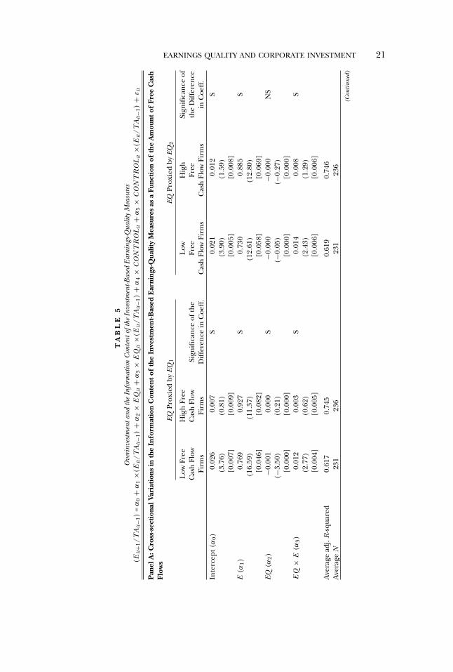
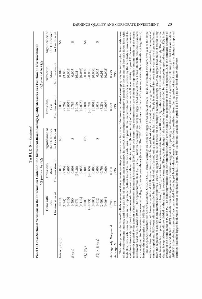
Panel A of table 5 presents the association of E Q 1 and E Q 2 with earn-ings persistence for firms with low and high free cash flows, respectively.I follow Richardson [2006] and calculate free cash flow as cash flow gen-erated from assets in place minus expected new investment; I then definefirms in the top tercile of free cash flows as high overinvestment tendencyfirms. The evidence in panel A of table 5 is consistent with the ex ante pre-diction that overinvesting firms tend to have less informative investment-based earnings-quality measures. For instance, the coefficient on E Q 1 ×E is 0.012 (t = 2.77) for firms in the bottom tercile of free cash flows and0.003 (t = 0.62) for those in the top tercile; the difference is also statisticallysignificant at the 10% level.
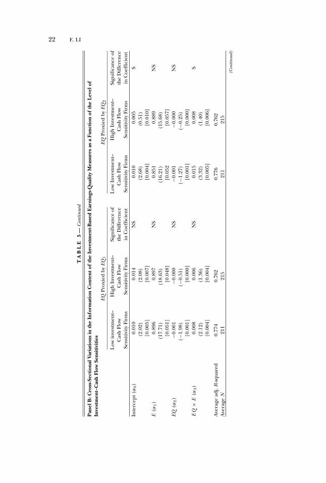
Panel B of table 5 measures the overinvestment tendency by using thesensitivity of investment to the amount of free cash flows measured for eachfirm year using data from the last 10 years. Based on the findings in Richard-son [2006], firms that tend to overinvest have higher investment–cash flowsensitivity.11 Results in panel B of table 5 are largely consistent with thisreasoning. The coefficient on E Q 2 × E is 0.015 (t = 3.32) for the lowinvestment–cash flow sensitivity firms, much higher than that for firms withhigh investment–cash flow sensitivity (0.008 with t = 1.40). For E Q 1 × E ,this difference is also positive (0.008 vs. 0.006), although it is smaller andstatistically insignificant.
In Panel C of table 5, I rely directly on the overinvestment measureconstructed by Richardson [2006] for the cross-sectional tests. Becausethis measure directly relates to capital expenditure, I focus on the capitalinvestment-based earnings-quality measures. I calculate overinvestment asthe residual from a regression of new capital investment on growth oppor-tunities, leverage, cash, firm age, size, stock returns, lagged investment, year
11 The finance literature has argued that firms with higher investment–cash flow sensitivitytend to have more severe financing constraint. Nevertheless, this interpretation also leads toa prediction of suboptimal investment for firms with higher investment–cash flow sensitivity.
EARNINGS QUALITY AND CORPORATE INVESTMENT 21
TA
BL
E5
Ove
rinv
estm
enta
ndth
eIn
form
atio
nC
onte
ntof
the
Inve
stm
ent-B
ased
Earn
ings
-Qua
lity
Mea
sure
s(E
it+1
/TA
it−1
)=
α0
+α
1×(
Eit
/TA
it−1
)+
α2
×E
Qit
+α
3×
EQ
it×(
Eit
/TA
it−1
)+
α4
×C
ON
TR
OL
it+
α5
×C
ON
TR
OL
it×(
Eit
/TA
it−1
)+
εit
Pan
elA
:Cro
ss-s
ecti
onal
Vari
atio
nsin
the
Info
rmat
ion
Con
tent
ofth
eIn
vest
men
t-Bas
edE
arni
ngs-
Qua
lity
Mea
sure
sas
aFu
ncti
onof
the
Am
ount
ofFr
eeC
ash
Flow
sEQ
Prox
ied
byEQ
1EQ
Prox
ied
byEQ
2
Low
Free
Hig
hFr
eeL
owH
igh
Sign
ifica
nce
ofC
ash
Flow
Cas
hFl
owSi
gnifi
canc
eof
the
Free
Free
the
Diff
eren
ceFi
rms
Firm
sD
iffer
ence
inC
oeff
.C
ash
Flow
Firm
sC
ash
Flow
Firm
sin
Coe
ff.
Inte
rcep
t(α
0)0.
026
0.00
7S
0.02
10.
012
S(3
.76)
(0.8
1)(3
.90)
(1.5
9)[0
.007
][0
.009
][0
.005
][0
.008
]E
(α1)
0.76
90.
927
S0.
730
0.88
5S
(16.
59)
(11.
37)
(12.
61)
(12.
80)
[0.0
46]
[0.0
82]
[0.0
58]
[0.0
69]
EQ(α
2)−0
.001
0.00
0S
−0.0
00−0
.000
NS
(−3.
50)
(0.2
1)(−
0.05
)(−
0.27
)[0
.000
][0
.000
][0
.000
][0
.000
]E
Q×
E(α
3)0.
012
0.00
3S
0.01
40.
008
S(2
.77)
(0.6
2)(2
.43)
(1.2
9)[0
.004
][0
.005
][0
.006
][0
.006
]
Ave
rage
adj.
R-sq
uare
d0.
617
0.74
50.
619
0.74
6A
vera
geN
231
236
231
236
(Con
tinue
d)
22 F. LI
TA
BL
E5
—C
ontin
ued
Pan
elB
:Cro
ss-S
ecti
onal
Vari
atio
nsin
the
Info
rmat
ion
Con
tent
ofth
eIn
vest
men
t-Bas
edE
arni
ngs-
Qua
lity
Mea
sure
sas
aFu
ncti
onof
the
Lev
elof
Inve
stm
ent–
Cas
hFl
owSe
nsit
ivit
ies
EQPr
oxie
dby
EQ1
EQPr
oxie
dby
EQ2
Low
inve
stm
ent–
Hig
hIn
vest
men
t–Si
gnifi
canc
eof
Low
Inve
stm
ent–
Hig
hIn
vest
men
t–Si
gnifi
canc
eof
Cas
hFl
owC
ash
Flow
the
Diff
eren
ceC
ash
Flow
Cas
hFl
owth
eD
iffer
ence
Sens
itivi
tyFi
rms
Sens
itivi
tyFi
rms
inC
oeffi
cien
tSe
nsiti
vity
Firm
sSe
nsiti
vity
Firm
sin
Coe
ffici
ent
Inte
rcep
t(α
0)
0.01
00.
014
NS
0.01
00.
005
S(2
.02)
(2.0
8)(2
.68)
(0.5
1)[0
.005
][0
.007
][0
.004
][0
.010
]E
(α1)
0.89
60.
897
NS
0.85
10.
889
NS
(17.
71)
(18.
63)
(16.
21)
(15.
68)
[0.0
51]
[0.0
48]
[0.0
52[0
.057
]EQ
(α2)
−0.0
01−0
.000
NS
−0.0
01−0
.000
NS
(−1.
98)
(−0.
51)
(−1.
27)
(−0.
25)
[0.0
01]
[0.0
00]
[0.0
01]
[0.0
00]
EQ
×E
(α3)
0.00
80.
006
NS
0.01
50.
008
S(2
.12)
(1.3
6)(3
.32)
(1.4
0)[0
.004
][0
.004
][0
.005
][0
.006
]
Ave
rage
adj.
R-sq
uare
d0.
774
0.76
20.
776
0.76
2A
vera
geN
211
215
211
215
(Con
tinue
d)
EARNINGS QUALITY AND CORPORATE INVESTMENT 23T
AB
LE
5—
Con
tinue
d
Pan
elC
:Cro
ss-S
ecti
onal
Vari
atio
nsin
the
Info
rmat
ion
Con
tent
ofth
eIn
vest
men
t-Bas
edE
arni
ngs-
Qua
lity
Mea
sure
sas
aFu
ncti
onof
Ove
rinv
estm
ent
EQpr
oxie
dby
EQ1
EQpr
oxie
dby
EQ2
Firm
sw
ithFi
rms
with
Sign
ifica
nce
ofFi
rms
with
Firm
sw
ithSi
gnifi
canc
eof
Les
sM
ore
the
Diff
eren
ceL
ess
Mor
eth
eD
iffer
ence
Ove
rinv
estm
ent
Ove
rinv
estm
ent
inC
oeffi
cien
tO
veri
nves
tmen
tO
veri
nves
tmen
tin
Coe
ffici
ent
Inte
rcep
t(α
0)0.
019
0.01
6N
S0.
016
0.01
6N
S(1
.94)
(2.9
5)(2
.26)
(3.0
3)[0
.010
][0
.005
][0
.007
][0
.005
]E
(α1)
0.79
00.
908
S0.
783
0.90
7S
(6.9
7)(1
6.36
)(1
0.10
)(1
6.31
)[0
.113
][0
.056
][0
.078
][0
.056
]EQ
(α2)
−0.0
01−0
.000
NS
−0.0
01−0
.000
NS
(−0.
93)
(−0.
63)
(−0.
79)
(−0.
80)
[0.0
01]
[0.0
00]
[0.0
01]
[0.0
00]
EQ
×E
(α3)
0.01
20.
003
S0.
018
0.00
5S
(2.6
9)(0
.76)
(3.2
3)(0
.91)
[0.0
04]
[0.0
04]
[0.0
06]
[0.0
05]
Ave
rage
adj.
R-sq
uare
d0.
708
0.78
00.
723
0.77
3A
vera
geN
233
235
233
235
Thi
sta
ble
pres
ents
the
Fam
a–M
acB
eth
regr
essi
ons
that
estim
ate
earn
ings
pers
iste
nce
asa
func
tion
ofth
ein
vest
men
t-bas
edea
rnin
gsqu
ality
for
two
sam
ples
:firm
sw
ithm
ore
ofan
over
inve
stm
ent
tend
ency
and
firm
sw
ithle
ssof
anov
erin
vest
men
tte
nden
cy.I
npa
nelA
,the
over
inve
stm
ent
tend
ency
ispr
oxie
dby
the
amou
ntof
free
cash
flow
s;fir
ms
with
high
(low
)fr
eeca
shfl
ows
are
thos
ein
the
top
terc
ile(b
otto
mte
rcile
)of
the
free
cash
flow
s.In
pane
lB,t
heov
erin
vest
men
tte
nden
cyis
prox
ied
byth
ese
nsiti
vity
ofin
vest
men
tto
cash
flow
s;fir
ms
with
high
(low
)in
vest
men
t–ca
shfl
owse
nsiti
vity
are
thos
ein
the
top
terc
ile(b
otto
mte
rcile
)of
the
inve
stm
ent–
cash
flow
sens
itivi
ty.I
npa
nelC
,the
over
inve
stm
ent
tend
ency
ispr
oxie
dby
the
amou
ntof
over
inve
stm
entf
ollo
win
gR
icha
rdso
n[2
006]
.Fir
ms
with
mor
e(l
ess)
over
inve
stm
enta
reth
ose
inth
eto
pte
rcile
(bot
tom
terc
ile)
ofth
eex
cess
inve
stm
entb
ased
onR
icha
rdso
n[2
006]
.The
depe
nden
tvar
iabl
eis
Eit+1
/TA
it−1
,nex
tyea
r’s
earn
ings
scal
edby
the
lagg
edbo
okva
lue
ofas
sets
.Fam
a–M
acB
eth
t-sta
tistic
s(s
tand
ard
erro
rs)
adju
sted
for
New
ey–W
est
auto
corr
elat
ion
(lag
=3)
are
inpa
rent
hese
s(b
rack
ets)
.The
“NS”
(“S”
)in
dica
tes
that
the
coef
ficie
nts
are
stat
istic
ally
nons
igni
fican
t(s
igni
fican
t)be
twee
nth
etw
osa
mpl
esat
the
10%
leve
l.T
hein
depe
nden
tvar
iabl
esar
ede
fined
asfo
llow
s.E
isE
it/T
Ait−1
,cur
rent
earn
ings
scal
edby
the
lagg
edbo
okva
lue
ofas
sets
.The
βC
ises
timat
edfo
rev
ery
firm
year
asth
esl
ope
coef
ficie
ntfr
omth
ere
gres
sion
ofch
ange
inca
pita
land
R&
Dex
pend
iture
s(s
cale
dby
lagg
edbo
okva
lue
ofas
sets
)on
the
chan
gein
repo
rted
earn
ings
(adj
uste
dfo
rth
eim
pact
ofcu
rren
tca
pita
land
R&
Dex
pend
iture
san
dsc
aled
byla
gged
book
valu
eof
asse
ts)
usin
gda
tafr
omth
ela
st10
year
s.T
heβ
Lis
estim
ated
for
ever
yfir
mye
aras
the
slop
eco
effic
ient
from
the
regr
essi
onof
chan
gein
the
num
ber
ofem
ploy
ees
(sca
led
byla
gged
book
valu
eof
asse
ts)
onth
ech
ange
inre
port
edea
rnin
gs(s
cale
dby
lagg
edbo
okva
lue
ofas
sets
)us
ing
data
from
the
last
10ye
ars.
For
afir
mye
arto
have
βC
and
βL
,it
mus
tha
veno
nmis
sing
data
for
the
last
10ye
ars.
EQ1
isth
eav
erag
eof
the
deci
lera
nks
ofβ
Can
dβ
LT
heγ
Cis
the
chan
gein
capi
tale
xpen
ditu
redi
vide
dby
the
chan
gein
repo
rted
earn
ings
.The
γL
isth
ech
ange
inth
enu
mbe
rof
empl
oyee
sdi
vide
dby
the
chan
gein
repo
rted
earn
ings
.EQ
2is
the
aver
age
ofth
ede
cile
rank
sof
γC
and
γL
.The
follo
win
gva
riab
les
and
thei
rin
tera
ctio
nsw
ithE
are
incl
uded
inth
ere
gres
sion
sbu
tare
notr
epor
ted.
DD
isth
est
anda
rdde
viat
ion
ofth
eD
echo
wan
dD
iche
v[2
002]
resi
dual
sfr
omth
ere
gres
sion
ofac
crua
lson
lagg
edC
FO(o
pera
ting
cash
flow
s),c
urre
ntC
FO,a
ndne
xtye
ar’s
CFO
usin
gth
ela
st10
year
sof
data
.A
BSA
CC
isth
eab
solu
team
ount
ofac
crua
ls,s
cale
dby
the
lagg
edbo
okva
lue
ofas
sets
.βR
isth
esl
ope
coef
ficie
ntfr
omth
ere
gres
sion
ofst
ock
retu
rns
onth
ech
ange
inre
port
edea
rnin
gs(s
cale
dby
lagg
edbo
okva
lue
ofas
sets
)us
ing
data
from
the
last
10ye
ars.
DIV
isa
dum
my
vari
able
that
equa
ls1
ifa
firm
pays
divi
dend
and
0ot
herw
ise.
24 F. LI
fixed effects, and the Fama–French 43 industry fixed effects. I then dividethe sample into firms with more overinvestment and less overinvestmentgroups. The results indicate that, consistent with the hypothesis, for firmswith less overinvestment problems, the interaction of E Q 1 with earningshas a coefficient of 0.012 (t = 2.69) and that for firms with more overin-vestment problems is 0.003 (t = 0.76), and the difference is statistically sig-nificant. Similarly, the coefficient on E Q 2 × E is higher for firms with lessoverinvestment. Overall, the evidence is largely consistent with the hypoth-esis that investment-based earnings-quality measures are more informativefor firms with less of an overinvestment tendency.
4.3 ADDITIONAL TESTS
4.3.1. Frequency of Earnings Increases and the Investment-Based Earnings Qual-ity. The accounting literature has documented the different implications oflosses for earnings properties (e.g., Hayn [1995]). In this subsection, I sys-tematically examine the relation between losses and the frequency of earn-ings increases versus decreases and the investment-based earnings-qualitymeasures.
First, to the extent that losses and earnings decreases are more likely to betemporary (Hayn [1995]), βC and βL should be lower for firms with morelosses or higher frequency of earnings decreases. For instance, because ofthe abandonment option, earnings decreases and losses are temporary and,as a result, I expect that investment decisions respond less to earnings de-creases or losses and hence the association between earnings and invest-ment is less positive. The results in panel A of table 6 strongly support thisargument: βC and βL both increase in the percentage of earnings increasesand decrease in the percentage of reported losses in the estimation window(last 10 years).
Second, I examine whether the association between investment-basedearnings-quality measures and earnings persistence is more significant ifI only include the positive βC and βL in the analysis. For instance, the statis-tics in table 1 show that more than 25% of the estimated βC ’s are negative.These negative βC estimates can be due to losses or earnings decreases asdiscussed in the previous paragraph. Panel B of table 6 presents the resultswhen the tests exclude firms with negative estimates of βL and βC . Com-pared with the results in table 4, the results are stronger in economic mag-nitude. For instance, the coefficient on βC × E is 0.057 (t = 4.30), muchlarger than that of 0.041 (t = 3.66) documented in table 4.
Also, I partition firm years into those that experienced few earnings in-creases in the last 10 years (our estimation window for βC and βL) andthose with more earnings increases. The prediction here is that for firmswith many earnings decreases, the investment-based earnings-quality mea-sures (βC and βL) are less informative compared with those with mostlyearnings increases in the estimation period. The results in panel C of table6 are consistent with this hypothesis: the coefficient on E Q × E is positiveand significant for firms with high frequency of earnings increases and isinsignificant for those with a high frequency of earnings decreases.
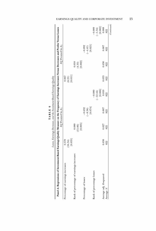
EARNINGS QUALITY AND CORPORATE INVESTMENT 25
TA
BL
E6
Los
ses,
Earn
ings
Dec
reas
es,a
ndth
eIn
vest
men
t-Bas
edEa
rnin
gsQ
ualit
y
Pan
elA
:Reg
ress
ions
ofIn
vest
men
t-Bas
edE
arni
ngs-
Qua
lity
Mea
sure
onth
eFr
eque
ncy
ofE
arni
ngs
Incr
ease
sVe
rsus
Dec
reas
esan
dP
rofi
tsVe
rsus
Los
ses
EQPr
oxie
dby
βC
EQPr
oxie
dby
βL
Perc
enta
geof
earn
ings
incr
ease
s0.
570
0.06
7(1
6.34
)(6
.21)
[0.0
35]
[0.0
11]
Ran
kof
perc
enta
geof
earn
ings
incr
ease
s0.
080
0.01
0(1
5.06
)(4
.33)
[0.0
05]
[0.0
02]
Perc
enta
geof
loss
es−0
.632
−0.0
92(−
8.56
)(−
4.41
)[0
.074
][0
.021
]R
ank
ofpe
rcen
tage
loss
es−0
.080
−0.0
09(−
12.4
4)(−
5.34
)[0
.006
][0
.002
]A
vera
gead
j.R
-squa
red
0.03
00.
027
0.00
70.
010
0.03
30.
030
0.00
70.
008
Ave
rage
N82
282
282
282
282
282
282
282
2(C
ontin
ued)
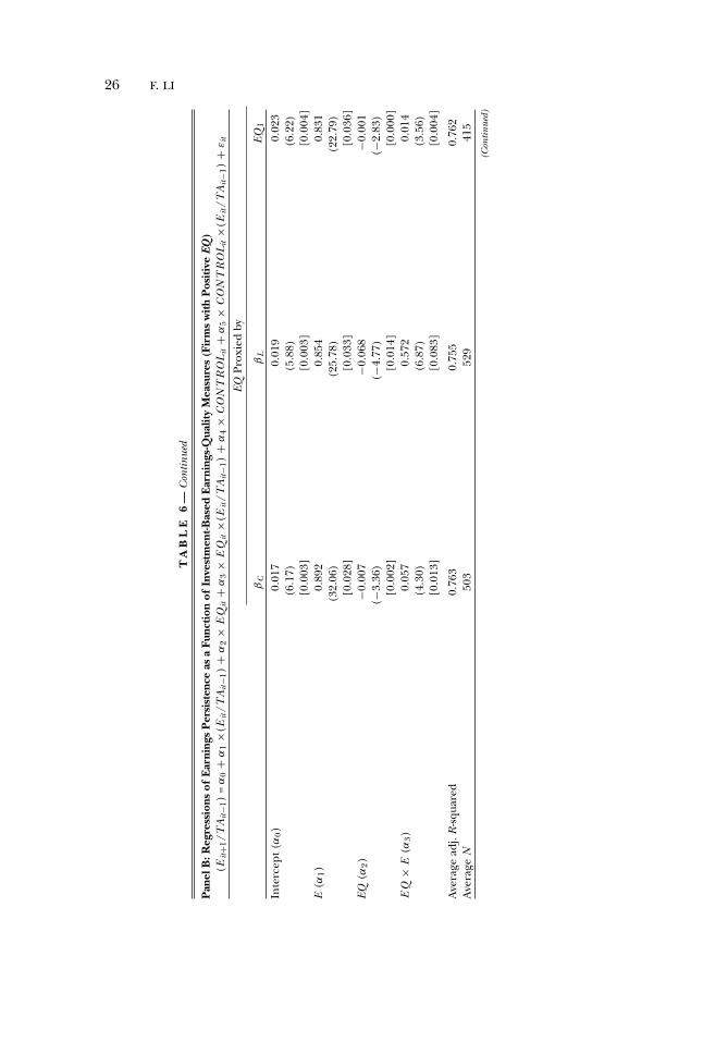
26 F. LI
TA
BL
E6
—C
ontin
ued
Pan
elB
:Reg
ress
ions
ofE
arni
ngs
Per
sist
ence
asa
Func
tion
ofIn
vest
men
t-Bas
edE
arni
ngs-
Qua
lity
Mea
sure
s(F
irm
sw
ith
Pos
itiv
eEQ
)(E
it+1
/TA
it−1
)=
α0
+α
1×(
Eit
/TA
it−1
)+
α2
×E
Qit
+α
3×
EQ
it×(
Eit
/TA
it−1
)+
α4
×C
ON
TR
OL
it+
α5
×C
ON
TR
OL
it×(
Eit
/TA
it−1
)+
εit
EQPr
oxie
dby
βC
βL
EQ1
Inte
rcep
t(α
0)
0.01
70.
019
0.02
3(6
.17)
(5.8
8)(6
.22)
[0.0
03]
[0.0
03]
[0.0
04]
E(α
1)
0.89
20.
854
0.83
1(3
2.06
)(2
5.78
)(2
2.79
)[0
.028
][0
.033
][0
.036
]EQ
(α2)
−0.0
07−0
.068
−0.0
01(−
3.36
)(−
4.77
)(−
2.83
)[0
.002
][0
.014
][0
.000
]E
Q×
E(α
3)
0.05
70.
572
0.01
4(4
.30)
(6.8
7)(3
.56)
[0.0
13]
[0.0
83]
[0.0
04]
Ave
rage
adj.
R-sq
uare
d0.
763
0.75
50.
762
Ave
rage
N50
352
941
5(C
ontin
ued)
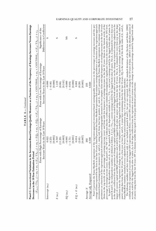
EARNINGS QUALITY AND CORPORATE INVESTMENT 27
TA
BL
E6
—C
ontin
ued
Pan
elC
:Cro
ss-s
ecti
onal
Vari
atio
nsin
the
Inve
stm
ent-B
ased
Ear
ning
s-Q
ualit
yM
easu
res
asa
Func
tion
ofth
eFr
eque
ncy
ofE
arni
ngs
Incr
ease
sVe
rsus
Ear
ning
sD
ecre
ases
inth
e10
-Yea
rE
stim
atio
nP
erio
d(E
it+1
/TA
it−1
)=
α0
+α
1×(
Eit
/TA
it−1
)+
α2
×E
Qit
+α
3×
EQ
it×(
Eit
/TA
it−1
)+
α4
×C
ON
TR
OL
it+
α5
×C
ON
TR
OL
it×(
Eit
/TA
it−1
)+
εit
Firm
sw
ithH
igh
Perc
enta
geof
Ear
ning
s-Fi
rms
with
Low
Perc
enta
geof
Ear
ning
s-Si
gnifi
canc
eof
the
Incr
ease
Year
sin
the
Las
t10
Year
sIn
crea
seYe
ars
inth
eL
ast1
0Ye
ars
Diff
eren
cein
Coe
ffici
ent
Inte
rcep
t(α
0)0.
021
−0.0
00S
(4.2
3)(−
0.46
)[0
.005
][0
.000
]E
(α1)
0.70
71.
133
S(1
1.29
)(8
.06)
[0.0
63]
[0.1
41]
EQ(α
2)−0
.001
−0.0
00N
S(−
1.71
)(−
0.04
)[0
.001
][0
.000
]E
Q×
E(α
3)0.
014
0.00
1S
(2.0
1)(0
.20)
[0.0
07]
[0.0
05]
Ave
rage
N20
223
3A
vera
gead
j.R
-squa
red
0.59
80.
820
Pane
lApr
esen
tsth
eFa
ma–
Mac
Bet
hre
gres
sion
sof
the
regr
essi
on-a
ppro
ach
inve
stm
ent-b
ased
earn
ings
-qua
lity
mea
sure
son
the
perc
enta
ges
ofea
rnin
gsin
crea
ses
and
the
per-
cent
age
oflo
sses
repo
rted
byth
efir
min
the
last
10ye
ars.
Pane
lBpr
esen
tsth
eFa
ma–
Mac
Bet
hre
gres
sion
stha
test
imat
eea
rnin
gspe
rsis
tenc
eas
afu
nctio
nof
the
regr
essi
on-a
ppro
ach
inve
stm
ent-b
ased
earn
ings
-qua
lity
mea
sure
s(β
Can
dβ
L),
usin
gon
lyfir
ms
that
have
posi
tive
βC
and
βL
.Pa
nel
Cpr
esen
tsth
eFa
ma–
Mac
Bet
hre
gres
sion
sth
ates
timat
eea
rnin
gspe
rsis
tenc
eas
afu
nctio
nof
the
regr
essi
on-a
ppro
ach
inve
stm
ent-b
ased
earn
ings
-qua
lity
mea
sure
sfo
rtw
osa
mpl
es:fi
rms
with
high
freq
uenc
yof
earn
ings
incr
ease
sin
the
last
10ye
ars
(firm
sin
the
top
terc
ileof
the
perc
enta
geof
earn
ings
incr
ease
year
s)an
dfir
ms
with
low
freq
uenc
yof
earn
ings
incr
ease
sin
the
last
10ye
ars
(firm
sin
the
bott
omte
rcile
ofth
epe
rcen
tage
ofea
rnin
gsin
crea
seye
ars)
.In
pane
lC,t
he“N
S”(“
S”)
indi
cate
stha
tthe
coef
ficie
ntsa
rest
atis
tical
lyno
nsig
nific
ant(
sign
ifica
nt)
betw
een
the
two
sam
ples
atth
e10
%le
vel.
Inpa
nelA
,the
depe
nden
tva
riab
les
are
βC
orβ
L.I
npa
nels
Ban
dC
,the
depe
nden
tva
riab
leis
Eit+1
/TA
it−1
,nex
tye
ar’s
earn
ings
scal
edby
the
lagg
edbo
okva
lue
ofas
sets
.In
pane
lsB
and
C,t
hein
depe
nden
tvar
iabl
esar
ede
fined
asfo
llow
s.E
isE
it/T
Ait−1
,cur
rent
earn
ings
scal
edby
the
lagg
edbo
okva
lue
ofas
sets
.The
βC
ises
timat
edfo
rev
ery
firm
year
asth
esl
ope
coef
ficie
ntfr
omth
ere
gres
sion
ofch
ange
inca
pita
land
R&
Dex
pend
iture
s(s
cale
dby
lagg
edbo
okva
lue
ofas
sets
)on
the
chan
gein
repo
rted
earn
ings
(adj
uste
dfo
rth
eim
pact
ofcu
rren
tca
pita
land
R&
Dex
pend
iture
san
dsc
aled
byla
gged
book
valu
eof
asse
ts)
usin
gda
tafr
omth
ela
st10
year
s.T
heβ
Lis
estim
ated
for
ever
yfir
mye
aras
the
slop
eco
effic
ient
from
the
regr
essi
onof
chan
gein
the
num
ber
ofem
ploy
ees
(sca
led
byla
gged
book
valu
eof
asse
ts)
onth
ech
ange
inre
port
edea
rnin
gs(s
cale
dby
lagg
edbo
okva
lue
ofas
sets
)us
ing
data
from
the
last
10ye
ars.
For
afir
mye
arto
have
βC
and
βL
,it
mus
tha
veno
nmis
sing
data
for
the
last
10ye
ars.
EQ1
isth
eav
erag
eof
the
deci
lera
nks
ofβ
Can
dβ
L.
Fam
a-M
acB
eth
t-sta
tistic
s(s
tand
ard
erro
rs)
adju
sted
for
New
ey–W
esta
utoc
orre
latio
n(l
ag=
3)ar
ein
pare
nthe
ses
(bra
cket
s).
The
follo
win
gva
riab
les
and
thei
rin
tera
ctio
nsw
ithE
are
incl
uded
inpa
nels
Ban
dC
,bu
tar
eno
tre
port
ed.
DD
isth
est
anda
rdde
viat
ion
ofth
eD
echo
wan
dD
iche
v[2
002]
resi
dual
sfr
omth
ere
gres
sion
ofac
crua
lson
lagg
edC
FO(o
pera
ting
cash
flow
s),c
urre
ntC
FO,a
ndne
xtye
ar’s
CFO
usin
gth
ela
st10
year
sof
data
.AB
SAC
Cis
the
abso
lute
amou
ntof
accr
uals
,sca
led
byth
ela
gged
book
valu
eof
asse
ts.β
Ris
the
slop
eco
effic
ient
from
the
regr
essi
onof
stoc
kre
turn
son
the
chan
gein
repo
rted
earn
ings
(sca
led
byla
gged
book
valu
eof
asse
ts)
usin
gda
tafr
omth
ela
st10
year
s.D
IVis
adu
mm
yva
riab
leth
ateq
uals
1if
afir
mpa
ysdi
vide
ndan
d0
othe
rwis
e.
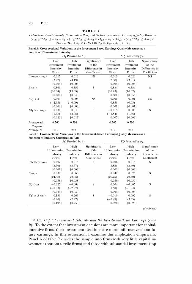
28 F. LI
T A B L E 7Capital-Investment Intensity, Unionization Rate, and the Investment-Based Earnings-Quality Measures(E it+1/TAit−1) = α0 + α1 ×(E it /TAit−1) + α2 × EQ it + α3 × E Q it ×(E it /TAit−1) + α4 ×
CON TROLit + α5 × CON TROLit ×(E it /TAit−1) + εit
Panel A: Cross-sectional Variations in the Investment-Based Earnings-Quality Measures as aFunction of Investment Intensity
EQ Proxied by βC EQ Proxied by γ C
Low High Significance Low High SignificanceInvestment Investment of the Investment Investment of the
Intensity Intensity Difference in Intensity Intensity Difference inFirms Firms Coefficient Firms Firms Coefficient
Intercept (α0) 0.015 0.019 NS 0.013 0.020 NS(3.22) (4.19) (2.88) (3.81)[0.005] [0.005] [0.005] [0.005]
E (α1) 0.865 0.856 S 0.884 0.854 S(10.34) (17.69) (10.93) (16.07)
[0.084] [0.048] [0.081] [0.053]EQ (α2) −0.005 −0.003 NS 0.001 0.001 NS
(−2.35) (−0.99) (0.85) (0.93)[0.002] [0.003] [0.001] [0.001]
E Q × E (α3) 0.030 0.040 S −0.013 0.003 S(1.38) (2.98) (−1.84) (1.66)[0.022] [0.013] [0.007] [0.002]
Average adj. 0.766 0.751 0.767 0.753R -squared
Average N 212 232 212 232Panel B: Cross-sectional Variations in the Investment-Based Earnings-Quality Measures as aFunction of Industry Unionization Rate
EQ Proxied by βL EQ Proxied by γ L
Low High Significance Low High SignificanceUnionization Unionization of the Unionization Unionization of the
Industry Industry Difference in Industry Industry Difference inFirms Firms Coefficient Firms Firms Coefficient
Intercept (α0) 0.007 0.015 S 0.006 0.014 S(5.30) (5.67) (3.85) (5.50)[0.001] [0.003] [0.002] [0.003]
E (α1) 0.938 0.866 S 0.942 0.875 S(24.48) (22.53) (26.25) (22.40)
[0.038] [0.038] [0.036] [0.039]EQ (α2) −0.027 −0.068 S 0.004 −0.005 S
(−0.93) (−2.27) (1.50) (−1.94)[0.029] [0.030] [0.003] [0.003]
E Q × E (α3) 0.185 0.766 S −0.010 0.097 S(0.96) (2.97) (−0.49) (3.35)[0.193] [0.258] [0.020] [0.029]
(Continued)
4.3.2. Capital Investment Intensity and the Investment-Based Earnings Qual-ity. To the extent that investment decisions are more important for capital-intensive firms, their investment decisions are more informative about fu-ture earnings. In this subsection, I examine this implication empirically.Panel A of table 7 divides the sample into firms with very little capital in-vestment (bottom tercile firms) and those with substantial investment (top
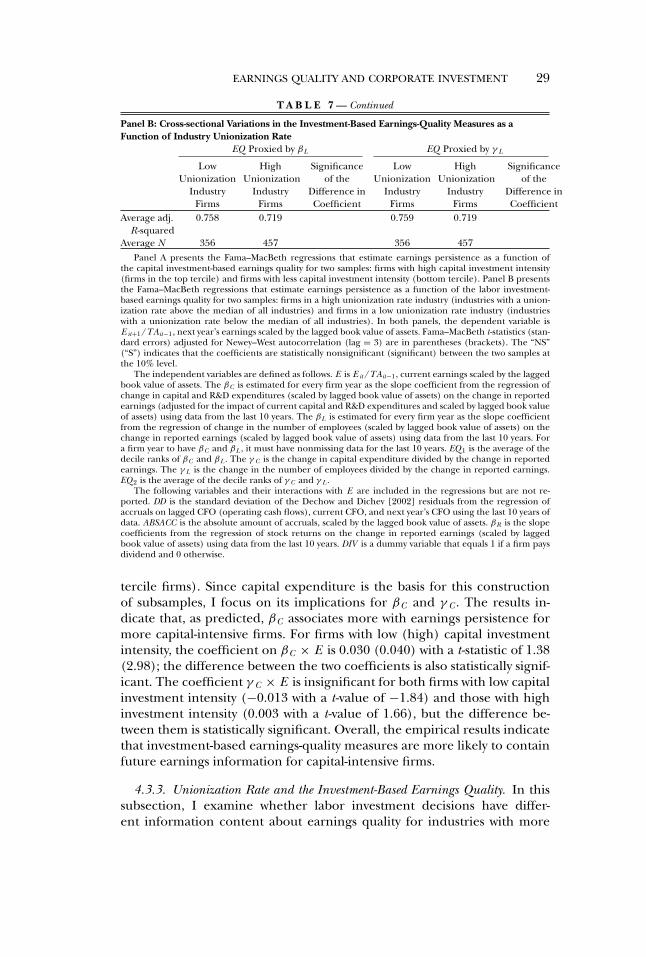
EARNINGS QUALITY AND CORPORATE INVESTMENT 29
T A B L E 7 — Continued
Panel B: Cross-sectional Variations in the Investment-Based Earnings-Quality Measures as aFunction of Industry Unionization Rate
EQ Proxied by βL EQ Proxied by γ L
Low High Significance Low High SignificanceUnionization Unionization of the Unionization Unionization of the
Industry Industry Difference in Industry Industry Difference inFirms Firms Coefficient Firms Firms Coefficient
Average adj. 0.758 0.719 0.759 0.719R -squared
Average N 356 457 356 457Panel A presents the Fama–MacBeth regressions that estimate earnings persistence as a function of
the capital investment-based earnings quality for two samples: firms with high capital investment intensity(firms in the top tercile) and firms with less capital investment intensity (bottom tercile). Panel B presentsthe Fama–MacBeth regressions that estimate earnings persistence as a function of the labor investment-based earnings quality for two samples: firms in a high unionization rate industry (industries with a union-ization rate above the median of all industries) and firms in a low unionization rate industry (industrieswith a unionization rate below the median of all industries). In both panels, the dependent variable isE it+1/TAit−1, next year’s earnings scaled by the lagged book value of assets. Fama–MacBeth t-statistics (stan-dard errors) adjusted for Newey–West autocorrelation (lag = 3) are in parentheses (brackets). The “NS”(“S”) indicates that the coefficients are statistically nonsignificant (significant) between the two samples atthe 10% level.
The independent variables are defined as follows. E is E it /TAit−1, current earnings scaled by the laggedbook value of assets. The βC is estimated for every firm year as the slope coefficient from the regression ofchange in capital and R&D expenditures (scaled by lagged book value of assets) on the change in reportedearnings (adjusted for the impact of current capital and R&D expenditures and scaled by lagged book valueof assets) using data from the last 10 years. The βL is estimated for every firm year as the slope coefficientfrom the regression of change in the number of employees (scaled by lagged book value of assets) on thechange in reported earnings (scaled by lagged book value of assets) using data from the last 10 years. Fora firm year to have βC and βL , it must have nonmissing data for the last 10 years. EQ 1 is the average of thedecile ranks of βC and βL . The γ C is the change in capital expenditure divided by the change in reportedearnings. The γ L is the change in the number of employees divided by the change in reported earnings.EQ 2 is the average of the decile ranks of γ C and γ L .
The following variables and their interactions with E are included in the regressions but are not re-ported. DD is the standard deviation of the Dechow and Dichev [2002] residuals from the regression ofaccruals on lagged CFO (operating cash flows), current CFO, and next year’s CFO using the last 10 years ofdata. ABSACC is the absolute amount of accruals, scaled by the lagged book value of assets. βR is the slopecoefficients from the regression of stock returns on the change in reported earnings (scaled by laggedbook value of assets) using data from the last 10 years. DIV is a dummy variable that equals 1 if a firm paysdividend and 0 otherwise.
tercile firms). Since capital expenditure is the basis for this constructionof subsamples, I focus on its implications for βC and γ C . The results in-dicate that, as predicted, βC associates more with earnings persistence formore capital-intensive firms. For firms with low (high) capital investmentintensity, the coefficient on βC × E is 0.030 (0.040) with a t-statistic of 1.38(2.98); the difference between the two coefficients is also statistically signif-icant. The coefficient γ C × E is insignificant for both firms with low capitalinvestment intensity (−0.013 with a t-value of −1.84) and those with highinvestment intensity (0.003 with a t-value of 1.66), but the difference be-tween them is statistically significant. Overall, the empirical results indicatethat investment-based earnings-quality measures are more likely to containfuture earnings information for capital-intensive firms.
4.3.3. Unionization Rate and the Investment-Based Earnings Quality. In thissubsection, I examine whether labor investment decisions have differ-ent information content about earnings quality for industries with more
30 F. LI
unionization. Prior empirical work based on both survey and historical datashows large wage differentials between union and nonunion workers withsimilar measured personal skills (Duncan and Stafford [1980]). Therefore,firms that hire more union employees likely pay a higher wage as comparedto nonunion firms, and union employees probably receive higher severancepay and benefits after being laid off as compared to nonunion employees.
This reasoning suggests that changes in employment levels are morecostly for firms that are heavily unionized. As a result, these firms needto be more certain that changes in demand are more permanent beforethey make changes in employment levels. Consequently, changes in em-ployment levels of heavily unionized firms are more informative about fu-ture earnings prospects. I hypothesize that the labor-based earnings-qualitymeasures are more informative about the future earnings.
Following Chen Kacperczyk and Ortiz-Molina [2010], I obtain unioniza-tion data for the period 1984-2004 from the Union Membership and Cover-age Database at www.unionstats.com, which is maintained by Barry Hirschand David Macpherson. The data are compiled from the Current Popu-lation Survey, based on the method used by the Bureau of Labor Statis-tics. Hirsch and Macpherson [2003] provide details on the constructionof this unique and comprehensive data set. I follow previous work in la-bor economics such as Connolly, Hirsch, and Hirschey [1986] and mea-sure labor force unionization as the percentage of employed workers in afirm’s primary Census Industry Classification (CIC) industry who are unionmembers.12 The data set comprises 188 CIC industries, which correspondroughly to three-digit SIC industries.
I define high (low) unionization industry as those industries with laborforce unionization rates above (below) the median of all industries. Theempirical results (table 7, panel B) show that, consistent with the predic-tion, the earnings-quality measure based on corporate labor investmentdecisions is more informative for firms from highly unionized industries:the coefficient on βL × E is 0.185 (t = 0.96) for firms in low unioniza-tion rate industries and 0.766 (t = 2.97) for those in high unionization rateindustries and the difference is statistically significant. Similar results areobtained for γ L.
4.3.4. Other Robustness Tests. One problem with using earnings persis-tence to gauge earnings quality is that next year’s earnings is of a short-termnature and captures the “permanent earnings” concept with error. To miti-gate this concern, I adopt an alternative specification by using longer termfuture cash flows as a measure of permanent earnings. Specifically, I sumthe cash flows from operations from year t + 1 to year t + 3 and regress thissum on earnings in year t to measure earnings persistence. I then examine
12 I also carry out another test based on the percentage of employees covered by unions inthe collective bargaining with the employers for a given industry and the (unreported) resultsare almost the same.
EARNINGS QUALITY AND CORPORATE INVESTMENT 31
whether the investment-based earnings-quality measures have implicationsfor the association of current earnings with future cash flows. Unreportedresults show that all the empirical results in the paper remain qualitativelysimilar. The results are also robust to an alternative definition of earningsand calculation of accruals and cash flows. For instance, the empirical re-sults remain similar if net income, instead of operating income, is used inthe tests. The empirical results still hold if industry-level definitions of earn-ings quality and earnings persistence are used.
5. Conclusion
In this study, I investigate a new approach to assess earnings quality,based on the reasoning that firm labor- and capital-investment decisionscontain managers’ information about future profitability. I document thatthere is a positive and significant relation between the investment-basedmeasures of earnings quality and earnings persistence. This effect holdsafter controlling for other commonly used measures of earnings quality.The information content in investment decisions with regard to futureearnings decreases with firms’ overinvestment tendency. The usefulness ofthe investment-based earnings-quality measures also varies with the capital-investment intensity, the unionization rate, and the frequency of earningsincreases versus decreases. Overall, the evidence from the paper suggeststhat it is important to tap into the information set of managers to assessearnings quality.
REFERENCES
BAKER, M. “Career Concerns and Staged Investment: Evidence from the Venture Capital In-dustry,” Working paper. Harvard Business School, 2000.
BASU, S. “The Conservatism Principle and the Asymmetric Timeliness of Earnings.” Journal ofAccounting and Economics 24 (1997): 3–37.
BEAVER, W. H. Financial Reporting: An Accounting Revolution, Third edition. Englewood Cliffs:Prentice Hall, 1998.
BERLE, A., AND G. MEANS. The Modern Corporation and Private Property. New York: Macmillan,1932.
BERTRAND, M., AND S. MULLAINATHAN. “Enjoying the Quiet Life? Corporate Governance andManagerial Preferences.” Journal of Political Economy 111 (2003): 1043–75.
BLACK, F. “The Magic in Earnings: Economic Earnings Versus Accounting Earnings.” FinancialAnalysts Journal 36 (1980): 19–24.
BLANCHARD, O. J.; E. LOPEZ DE SILANES; AND A. SHLEIFER. “What Do Firms Do with Cash Wind-falls.” Journal of Financial Economics 36 (1994): 337–60.
CHEN, J.; M. KACPERCZYK; and H. ORTIZ-MOLINA. “Labor Unions, Operating Flexibility, andthe Cost of Equity.” Journal of Financial and Quantitative Analysis (2010): Forthcoming.
COLLINS, D. W.; E. L. MAYDEW; and I. S. WEISS. “Changes in the Value-Relevance of Earningsand Book Values over the Past Forty Years.” Journal of Accounting and Economics 24 (1999):39–67.
CONNOLLY, R.; B. HIRSCH; AND M. HIRSCHEY. “Union Rent Seeking, Intangible Capital, andMarket Value of the Firm.” The Review of Economics and Statistics 68 (1986): 567–77.
DECHOW, P. M., AND I. D. DICHEV. “The Quality of Accruals and Earnings: The Role of AccrualEstimation Errors.” Accounting Review 77 (2002): 35–59.
32 F. LI
DECHOW, P. M., AND C. M. SCHRAND. Earnings Quality, First edition. Virginia, Charlottesville:Research Foundation of CFA Institute, 2004.
DICHEV, I., AND W. TANG. “Earnings Volatility and Earnings Predictability.” Journal of Accountingand Economics 47 (2009): 160–81.
DONALDSON, G. Managing Corporate Wealth, New York: Praeger, 1984.DUNCAN, G. J., AND F. P. STAFFORD. “Do Union Members Receive Compensating Wage Differ-
entials.” American Economic Review 70 (1980): 355–71.ECKER, F.; J. FRANCIS; I. KIM; P. OLSSON; AND K. SCHIPPER. “A Returns-Based Representation of
Earnings Quality.” The Accounting Review 81 (2006): 749–80.FAMA, E. F., AND J. MACBETH. “Risk, Return and Equilibrium: Empirical Tests.” Journal of Politi-
cal Economy 81 (1973): 607–36.FRANCIS, J.; R. LAFOND; P. OLSSON; AND K. SCHIPPER. “The Market Pricing of Accruals Quality.”
Journal of Accounting and Economics 31 (2005): 295–327.FRANCIS, J., AND K. SCHIPPER. “Have Financial Statements Lost Their Relevance?” Journal of
Accounting Research 37 (1999): 319–52.HAYN, C. “Information Content of Losses.” Journal of Accounting and Economics 20 (1995):
125–53.HEALY, P. M., AND J. M. WAHLEN. “A Review of the Earnings Management Literature and Its
Implications for Standard Setting.” Accounting Horizons 13 (1999): 365–83.HIRSCH, B. T., AND D. A. MACPHERSON. “Union Membership and Coverage Database from the
Current Population Survey: Note.” Industrial and Labor Relations Review 56 (2003): 349–54.JENSEN, M. C. “Agency Costs of Free Cash Flow, Corporate Finance, and Takeovers.” The Amer-
ican Economic Review 76 (1986): 323–29.JENSEN, M. C., AND W. H. MECKLING. “Managerial Behavior, Agency Costs and Ownership Struc-
ture.” Journal of Financial Economics 3 (1976): 305–60.LEV, B., AND T. SOUGIANNIS. “The Capitalization, Amortization and Value-Relevance of R&D.”
Journal of Accounting and Economics 21 (1996): 107–38.LI, F. “Annual Report Readability, Current Earnings, and Earnings Persistence.” Journal of Ac-
counting and Economics 45 (2008): 221–47.NEWEY, W. K., AND K. D. WEST. “Automatic Lag Selection in Covariance Matrix Estimation.”
Review of Economic Studies 61 (1994): 631–53.OHLSON, J., AND X. ZHANG. “Earnings, Book Values, and Dividends in Equity Security Valua-
tion.” Journal of Accounting Research 36 (1998): 85–111.RICHARDSON, S. “Over-Investment of Free Cash Flow.” Review of Accounting Studies 11 (2006):
159–89.SKINNER, D. J., AND E. SOLTES. “What Do Dividends Tell Us About Earnings Quality.” Review of
Accounting Studies (2009): Forthcoming.SLOAN, R. “Do Stock Prices Fully Reflect Information in Accruals and Cash Flows About Future
Earnings?” Accounting Review 71 (1996): 289–15.STEIN, J. C. “Agency, Information, and Corporate Investment,” in Handbook of the Economics
of Finance, edited by G. M. Constantinides, M. Harris, and R. Stulz. North Holland: B.V.Elsevier, 2003: 111–65.
WILLIAMSON, O. E. The Economics of Discretionary Behavior: Managerial Objectives in a Theory of theFirm. Englewood Cliffs, NJ: Prentice Hall, 1964.