Capital Investment Decisions

18 -1

Capital Capital Investment Investment DecisionsDecisions

CHAPTERCHAPTER

18 -2

1. Explain what a capital investment decision is, and distinguish between independent and mutually exclusive capital investment decisions.

2. Compute the payback period and accounting rate of return for a proposed investment, and explain their roles in capital investment decisions.

3. Use net present value analysis for capital investment decisions involving independent projects.

ObjectivesObjectivesObjectivesObjectives

After studying this After studying this chapter, you should chapter, you should

be able to:be able to:

After studying this After studying this chapter, you should chapter, you should

be able to:be able to:

18 -3

4. Use the internal rate of return to assess the acceptability of independent projects.

5. Discuss the role and value of postaudits.6. Explain why NPV is better than IRR for capital

investment decisions involving mutually exclusive projects.

7. Convert gross cash flows to after-tax cash flows.8. Describe capital investment in the advanced

manufacturing environment.

ObjectivesObjectivesObjectivesObjectives

18 -4

Capital investment decisions are concerned with the process of

planning, setting goals and priorities, arranging financing,

and using certain criteria to select long-term assets.

18 -5

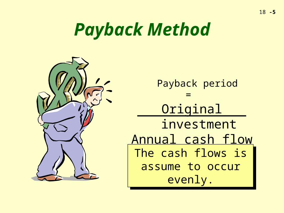
Payback Method

Payback period =

Original investmentAnnual cash flow

The cash flows is assume to occur evenly.

The cash flows is assume to occur evenly.

18 -6

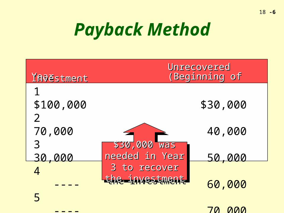
Payback Method

Year (Beginning of year) Annual Cash FlowYear (Beginning of year) Annual Cash Flow Unrecovered InvestmentUnrecovered Investment

1 $100,000 $30,0002 70,000 40,0003 30,000 50,0004 ---- 60,0005 ---- 70,000

$30,000 was needed $30,000 was needed in Year 3 to recover in Year 3 to recover

the investmentthe investment

$30,000 was needed $30,000 was needed in Year 3 to recover in Year 3 to recover

the investmentthe investment

18 -7

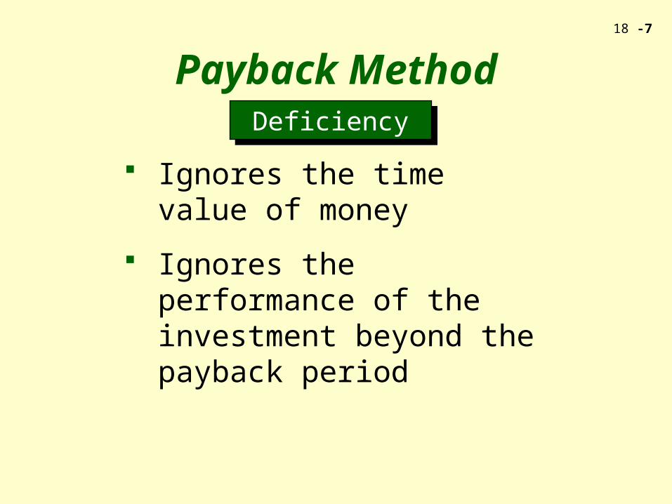
Ignores the time value of money

Ignores the performance of the investment beyond the payback period

Payback MethodDeficiencyDeficiency

18 -8

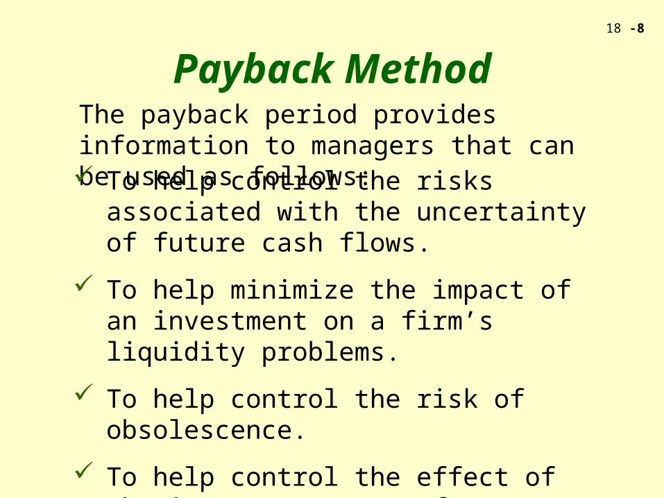
Payback MethodThe payback period provides information to managers that can be used as follows: To help control the risks associated with the

uncertainty of future cash flows.

To help minimize the impact of an investment on a firm’s liquidity problems.

To help control the risk of obsolescence.

To help control the effect of the investment on performance measures.

18 -9

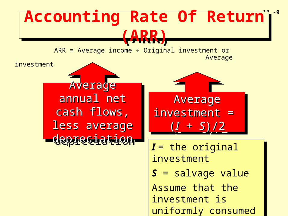
Accounting Rate Of Return (ARR)Accounting Rate Of Return (ARR)

ARR = Average income ÷ Original investment or Average investment

Average investment Average investment = (= (II + + SS)/2)/2

Average investment Average investment = (= (II + + SS)/2)/2

I = the original investment

S = salvage value

Assume that the investment is uniformly consumed

I = the original investment

S = salvage value

Assume that the investment is uniformly consumed

Average annual net Average annual net cash flows, less cash flows, less

average average depreciationdepreciation

Average annual net Average annual net cash flows, less cash flows, less

average average depreciationdepreciation

18 -10

Example: Suppose that some new equipment requires an initial outlay of $80,000 and promises total cash flows of $120,000 over the next five years (the life of the machine). What is the ARR?

Answer: The average cash flow is $24,000 ($120,000 ÷ 5) and the average depreciation is $16,000 ($80,000 ÷ 5).

ARR = ($24,000 – $16,000) ÷ $80,000 = $8,000 ÷ $80,000 = 10%


18 -11

A screening measure to ensure that new investment will not adversely affect net income

To ensure a favorable effect on net income so that bonuses can be earned (increased)

Reasons for Using ARRReasons for Using ARR


18 -12

The major deficiency of the accounting rate of return is that it ignores the time value of money.


18 -13

NPV = P – I

where:

P = the present value of the project’s future cash inflows

I = the present value of the project’s cost (usually the initial outlay)

Net present value is the difference between the present value of the cash inflows and outflows associated with a project.

The Net Present Value MethodThe Net Present Value MethodThe Net Present Value MethodThe Net Present Value Method

18 -14

Brannon Company has developed new earphones for portable CD and tape players that are expected to generate an annual revenue of $300,000. Necessary production equipment would cost $320,000 and can be sold in five years for $40,000.


18 -15

In addition, working capital is expected to increase by $40,000 and is expected to be recovered at the end of five years. Annual operating expenses are expected to be $180,000. The required rate of return is 12 percent.


18 -16

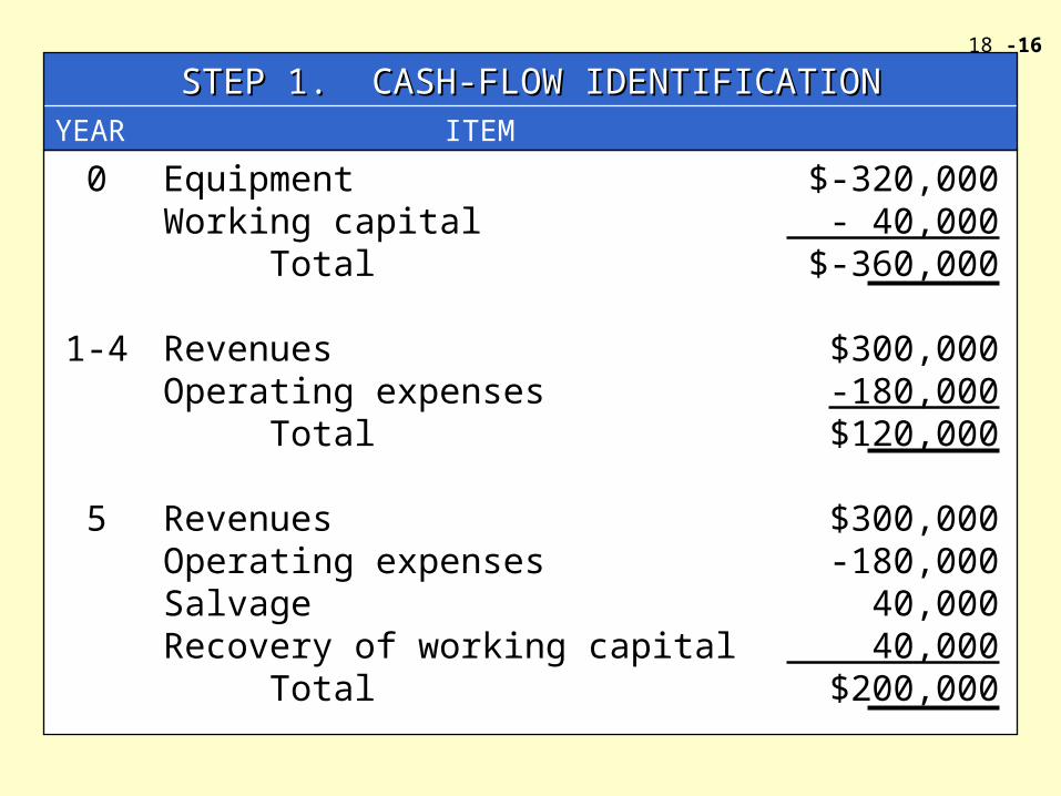
STEP 1. CASH-FLOW IDENTIFICATIONSTEP 1. CASH-FLOW IDENTIFICATIONYEAR ITEM CASH FLOW0 Equipment $-320,000

Working capital - 40,000 Total $-360,000

1-4 Revenues $300,000Operating expenses -180,000 Total $120,000

5 Revenues $300,000Operating expenses -180,000Salvage 40,000Recovery of working capital 40,000 Total $200,000

18 -17

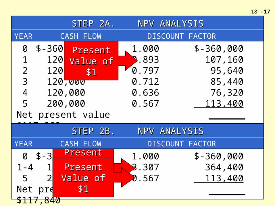
STEP 2A. NPV ANALYSISSTEP 2A. NPV ANALYSISYEAR CASH FLOW DISCOUNT FACTOR PRESENT VALUE

0 $-360,000 1.000 $-360,0001 120,000 0.893 107,1602 120,000 0.797 95,6403 120,000 0.712 85,4404 120,000 0.636 76,3205 200,000 0.567 113,400

Net present value $117,960

STEP 2B. NPV ANALYSISSTEP 2B. NPV ANALYSISYEAR CASH FLOW DISCOUNT FACTOR PRESENT VALUE

0 $-360,000 1.000 $-360,0001-4 120,000 3.307 364,4005 200,000 0.567 113,400

Net present value $117,840

Present Present Value of $1Value of $1

Present Value Present Value of an Annuity of an Annuity

of $1of $1Present Value Present Value

of $1of $1

18 -18

If NPV = 0, this indicates:

1. The initial investment has been recovered

2. The required rate of return has been recovered

Thus, break even has been achieved and we are indifferent about the project.


Decision Criteria for NPV

18 -19

Decision Criteria for NPV

If the NPV > 0 this indicates:

1. The initial investment has been recovered

2. The required rate of return has been recovered

3. A return in excess of 1. and 2. has been received

Thus, the earphones should be manufactured.


18 -20

Reinvestment Assumption

The NVP model assumes that all cash flows generated by a project are immediately reinvested to earn the required rate of return throughout the life of the project.


18 -21

The internal rate of return (IRR) is the discount rate that sets the project’s NPV at zero. Thus, P = I for the IRR.

Example: A project requires a $10,000 investment and will return $12,000 after one year. What is the IRR?

$12,000/(1 + i) = $10,000 1 + i = 1.2 i = 0.20

Internal Rate of ReturnInternal Rate of ReturnInternal Rate of ReturnInternal Rate of Return

18 -22

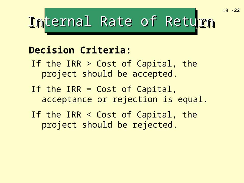
If the IRR > Cost of Capital, the project should be accepted.

If the IRR = Cost of Capital, acceptance or rejection is equal.

If the IRR < Cost of Capital, the project should be rejected.

Internal Rate of ReturnInternal Rate of ReturnInternal Rate of ReturnInternal Rate of Return

Decision Criteria:

18 -23

NPV Compared With IRR

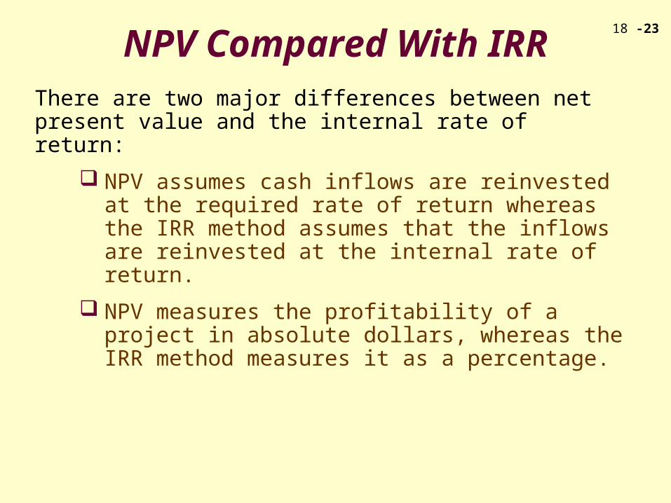
There are two major differences between net present value and the internal rate of return:

NPV assumes cash inflows are reinvested at the required rate of return whereas the IRR method assumes that the inflows are reinvested at the internal rate of return.

NPV measures the profitability of a project in absolute dollars, whereas the IRR method measures it as a percentage.

18 -24


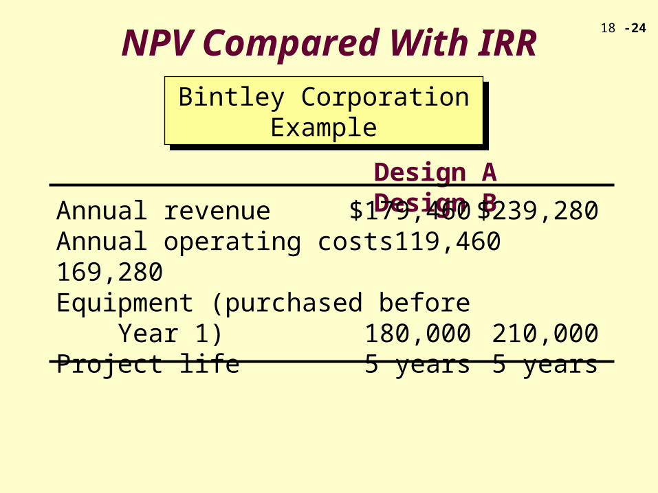
Design A Design B

Annual revenue $179,460 $239,280Annual operating costs 119,460 169,280Equipment (purchased before Year 1) 180,000 210,000Project life 5 years 5 years

Bintley Corporation ExampleBintley Corporation Example

18 -25

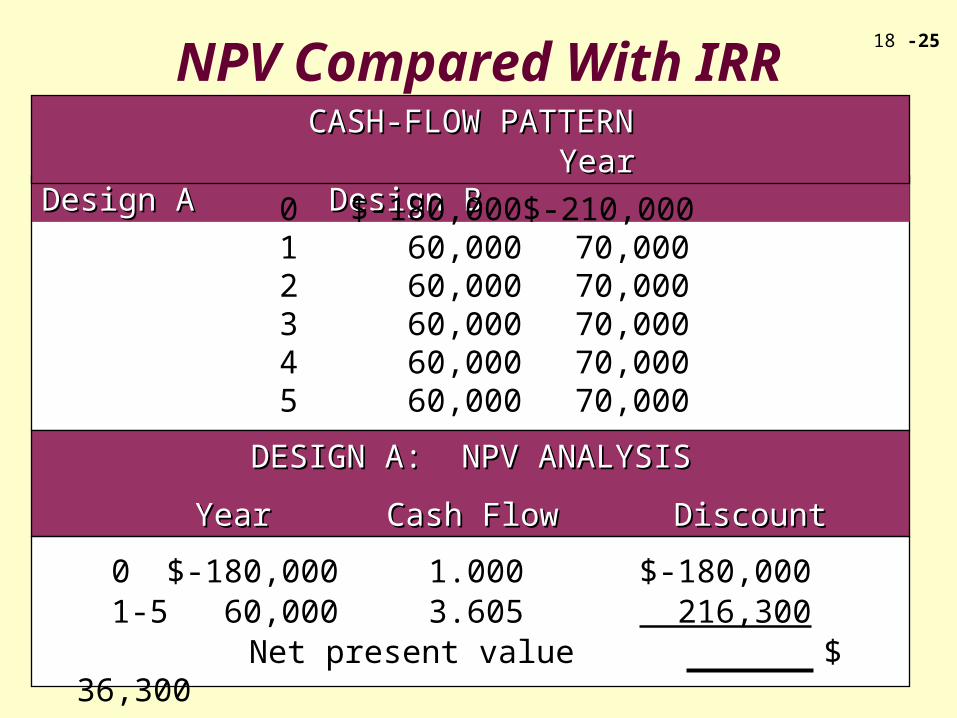
NPV Compared With IRRCASH-FLOW PATTERNCASH-FLOW PATTERN

Year Design A Design BYear Design A Design B

0 $-180,000 $-210,0001 60,000 70,0002 60,000 70,0003 60,000 70,0004 60,000 70,0005 60,000 70,000

DESIGN A: NPV ANALYSISDESIGN A: NPV ANALYSIS

Year Cash Flow Discount Factor Present ValueYear Cash Flow Discount Factor Present Value

0 $-180,000 1.000 $-180,0001-5 60,000 3.605 216,300

Net present value $ 36,300

18 -26

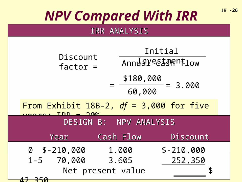
IRR ANALYSISIRR ANALYSIS

Discount factor =


Initial Investment

Annual cash flow

=$180,000

60,000

= 3,000From Exhibit 18B-2, df = 3,000 for five years; IRR = 20%

= 3.000

DESIGN B: NPV ANALYSISDESIGN B: NPV ANALYSIS


0 $-210,000 1.000 $-210,0001-5 70,000 3.605 252,350


18 -27

IRR ANALYSISIRR ANALYSIS

Discount factor =Initial Investment

Annual cash flow

=$210,000

70,000

= 3,000From Exhibit 18B-2, df = 3,000 for five years; IRR = 20%


= 3.000

18 -28

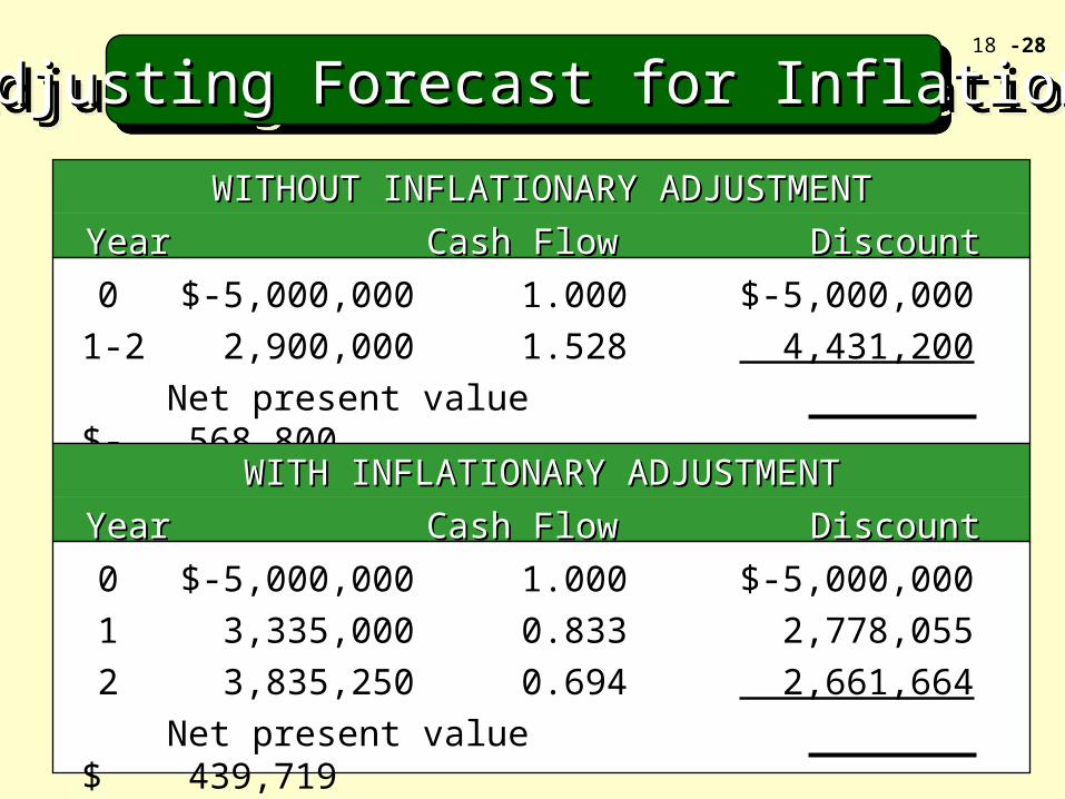
Adjusting Forecast for InflationAdjusting Forecast for InflationAdjusting Forecast for InflationAdjusting Forecast for Inflation

WITHOUT INFLATIONARY ADJUSTMENTWITHOUT INFLATIONARY ADJUSTMENT


0 $-5,000,000 1.000 $-5,000,000

1-2 2,900,000 1.528 4,431,200

Net present value $- 568,800

WITH INFLATIONARY ADJUSTMENTWITH INFLATIONARY ADJUSTMENT


0 $-5,000,000 1.000 $-5,000,000

1 3,335,000 0.833 2,778,055

2 3,835,250 0.694 2,661,664


18 -29

After-Tax Operating Cash Flows The Income Approach

After-tax cash flow = After-tax net income + Noncash expenses

Example:Revenues $1,000,000Less: Operating expenses* 600,000Income before taxes $ 400,000Less: Income taxes 136,000Net income $ 264,000

*$100,000 is depreciation

After-tax cash flow = $264,000 + $100,000

= $364,000

18 -30

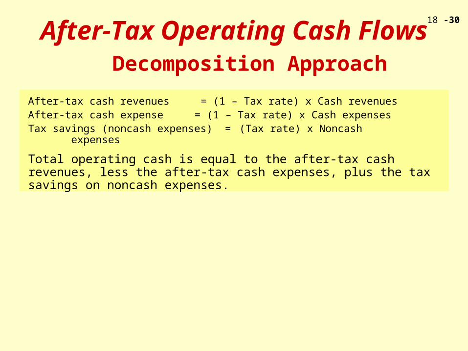
After-tax cash revenues = (1 – Tax rate) x Cash revenuesAfter-tax cash expense = (1 – Tax rate) x Cash expensesTax savings (noncash expenses) = (Tax rate) x Noncash

expenses

Total operating cash is equal to the after-tax cash revenues, less the after-tax cash expenses, plus the tax savings on noncash expenses.

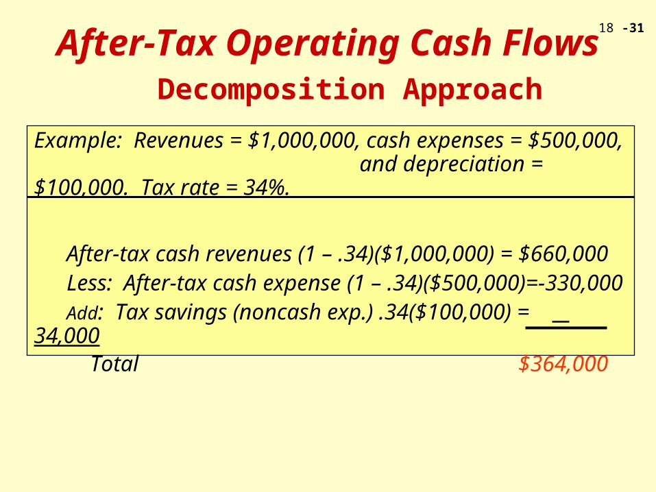
After-Tax Operating Cash Flows Decomposition Approach

18 -31

Example: Revenues = $1,000,000, cash expenses = $500,000, and depreciation = $100,000. Tax rate = 34%.

After-tax cash revenues (1 – .34)($1,000,000) = $660,000Less: After-tax cash expense (1 – .34)($500,000)= -330,000Add: Tax savings (noncash exp.) .34($100,000) = 34,000 Total $364,000

After-Tax Operating Cash Flows Decomposition Approach

18 -32

DepreciationTax-Shielding Effect


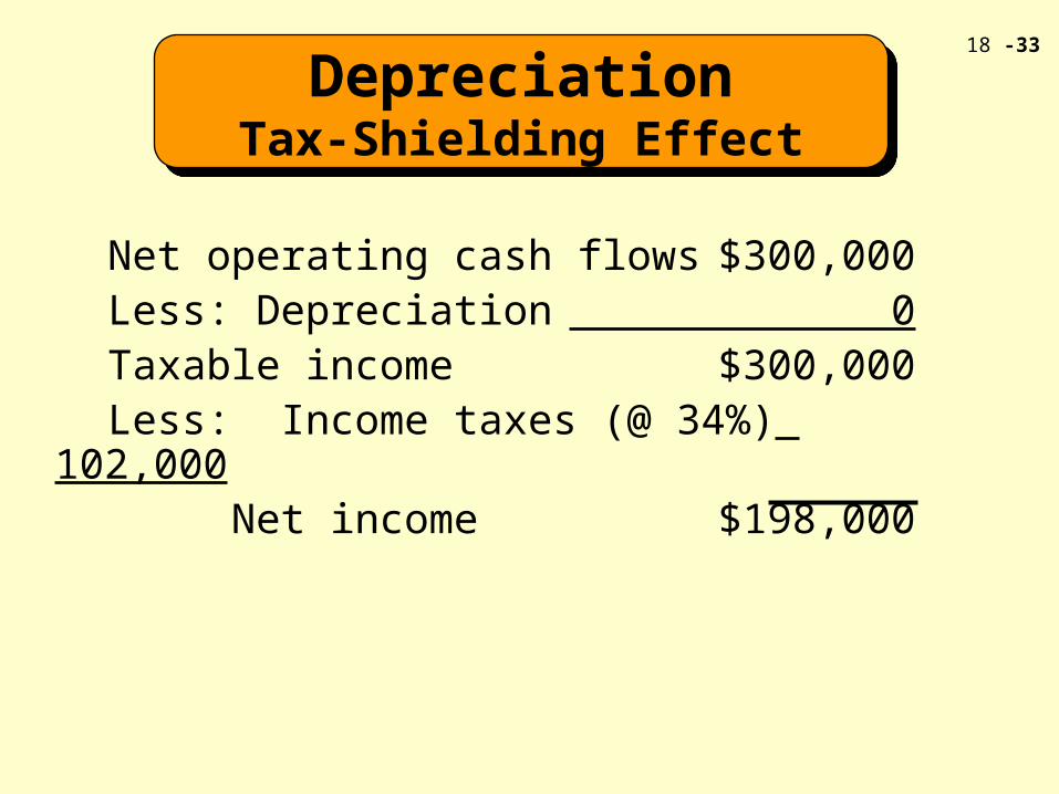
Depreciation is a noncash expense and is not a cash flow. Depreciation, however SHIELDS revenues from being taxed and, thus, creates a cash inflow

equal to the tax savings.

Assume initially that tax laws DO NOT allow depreciation to be deducted to arrive at taxable income. If a company had before-tax operating

cash flows of $300,000 and depreciation of $100,000, we have the statement found on Slide 33.

18 -33

Net operating cash flows $300,000Less: Depreciation 0Taxable income $300,000Less: Income taxes (@ 34%) 102,000 Net income $198,000



18 -34

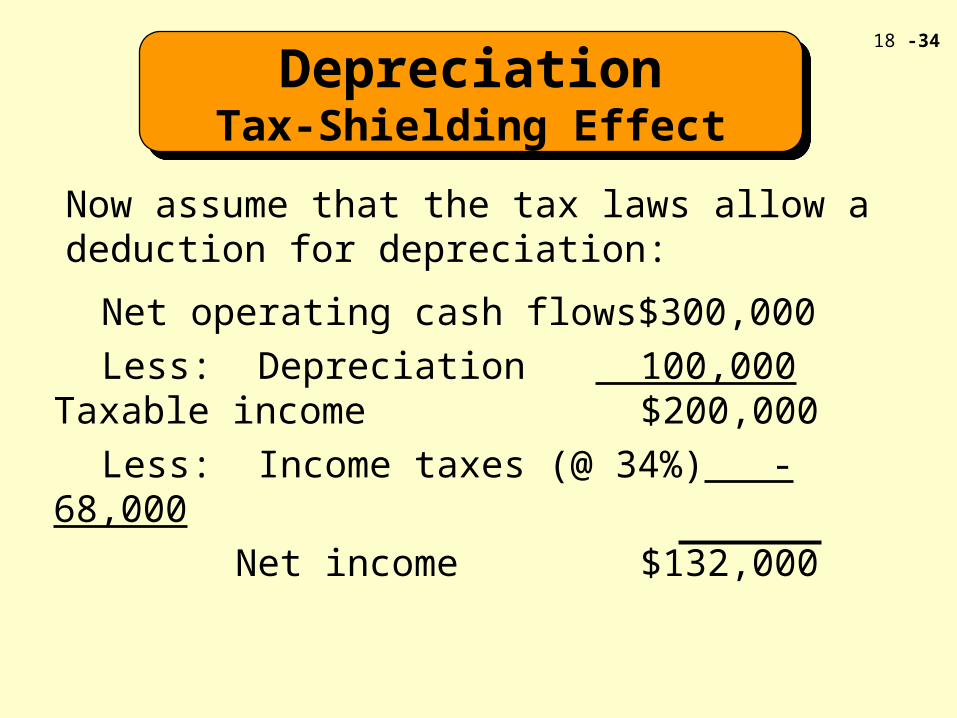
Net operating cash flows $300,000

Less: Depreciation 100,000 Taxable income $200,000

Less: Income taxes (@ 34%) -68,000

Net income $132,000



Now assume that the tax laws allow a deduction for depreciation:

18 -35

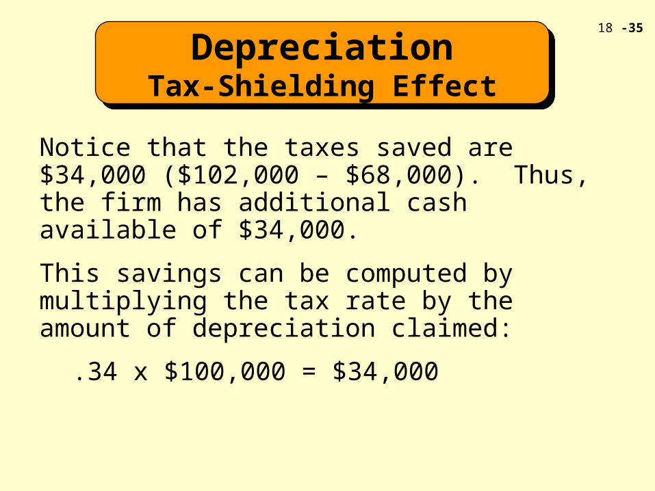
Notice that the taxes saved are $34,000 ($102,000 – $68,000). Thus, the firm has additional cash available of $34,000.

This savings can be computed by multiplying the tax rate by the amount of depreciation claimed:

.34 x $100,000 = $34,000



18 -36

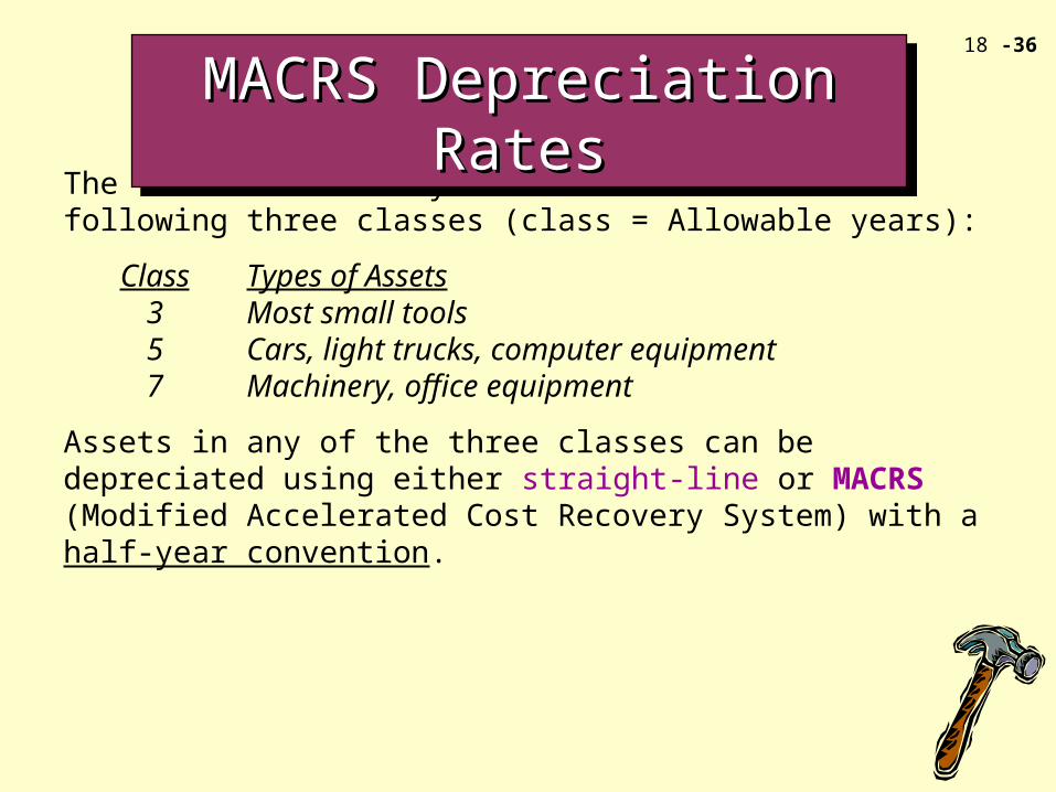
The tax laws classify most assets into the following three classes (class = Allowable years):

Class Types of Assets3 Most small tools5 Cars, light trucks, computer equipment7 Machinery, office equipment

Assets in any of the three classes can be depreciated using either straight-line or MACRS (Modified Accelerated Cost Recovery System) with a half-year convention.

MACRS Depreciation RatesMACRS Depreciation RatesMACRS Depreciation RatesMACRS Depreciation Rates

18 -37

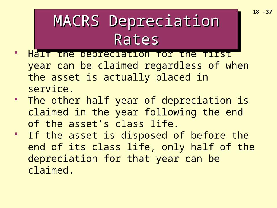
Half the depreciation for the first year can be claimed regardless of when the asset is actually placed in service.

The other half year of depreciation is claimed in the year following the end of the asset’s class life.

If the asset is disposed of before the end of its class life, only half of the depreciation for that year can be claimed.

MACRS Depreciation RatesMACRS Depreciation RatesMACRS Depreciation RatesMACRS Depreciation Rates

18 -38

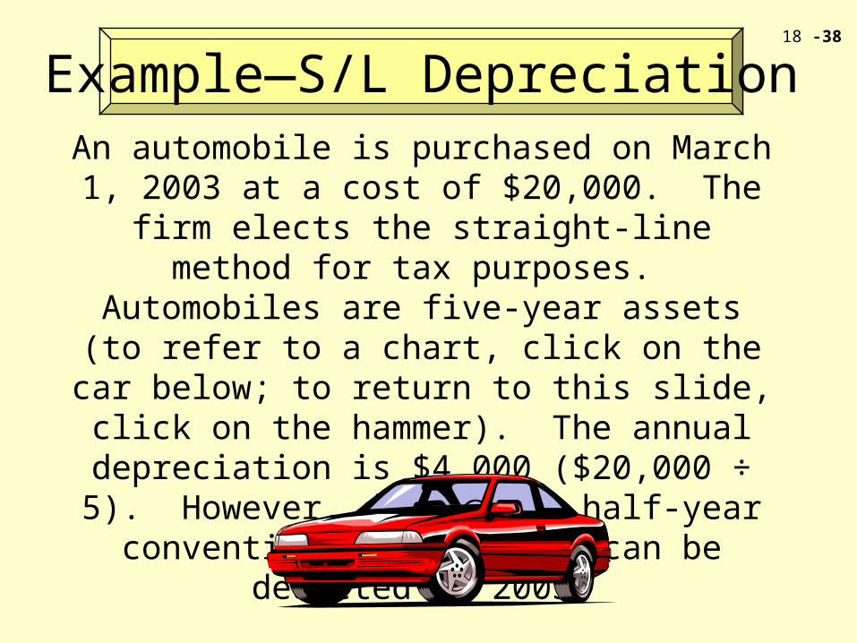
Example—S/L DepreciationAn automobile is purchased on March 1, 2003 at a cost of $20,000. The firm elects the straight-line

method for tax purposes. Automobiles are five-year assets (to refer to a chart, click on the car below; to

return to this slide, click on the hammer). The annual depreciation is $4,000 ($20,000 ÷ 5).

However, due to the half-year convention, only $2,000 can be deducted in 2003.

18 -39

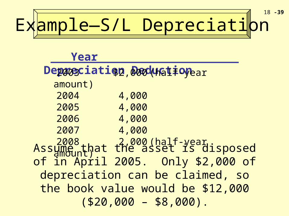
Year Depreciation Deduction2003 $2,000 (half-year amount)2004 4,0002005 4,0002006 4,0002007 4,0002008 2,000 (half-year amount)

Assume that the asset is disposed of in April 2005. Only $2,000 of depreciation can be claimed, so

the book value would be $12,000 ($20,000 – $8,000).

Example—S/L Depreciation

18 -40

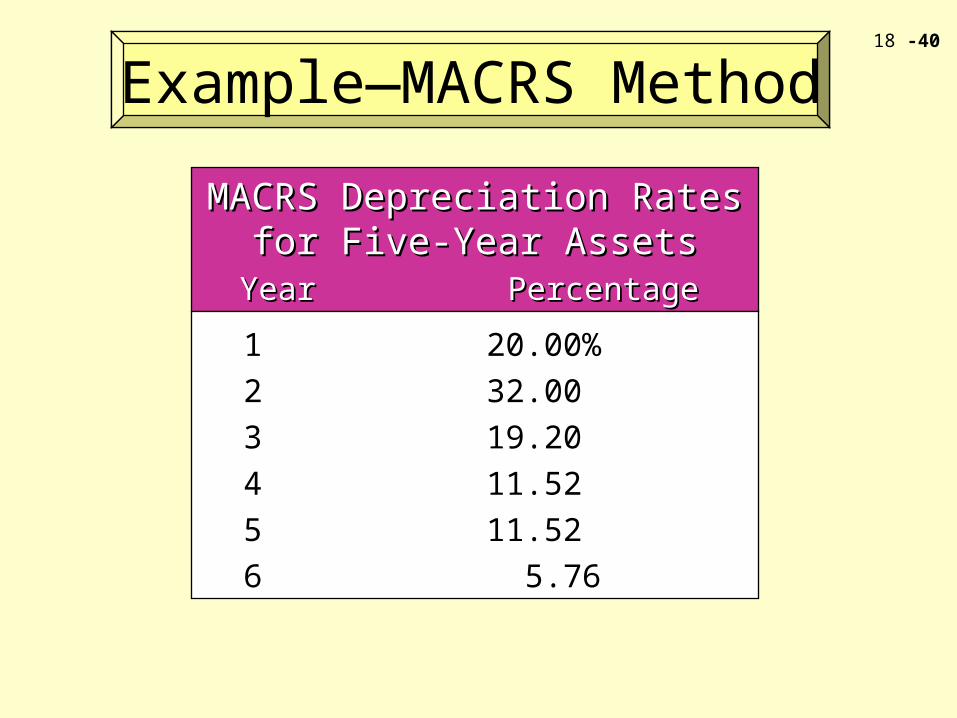
Example—MACRS Method

MACRS Depreciation Rates for MACRS Depreciation Rates for Five-Year AssetsFive-Year Assets

Year Percentage of Cost AllowedYear Percentage of Cost Allowed

1 20.00%

2 32.00

3 19.20

4 11.52

5 11.52

6 5.76

18 -41

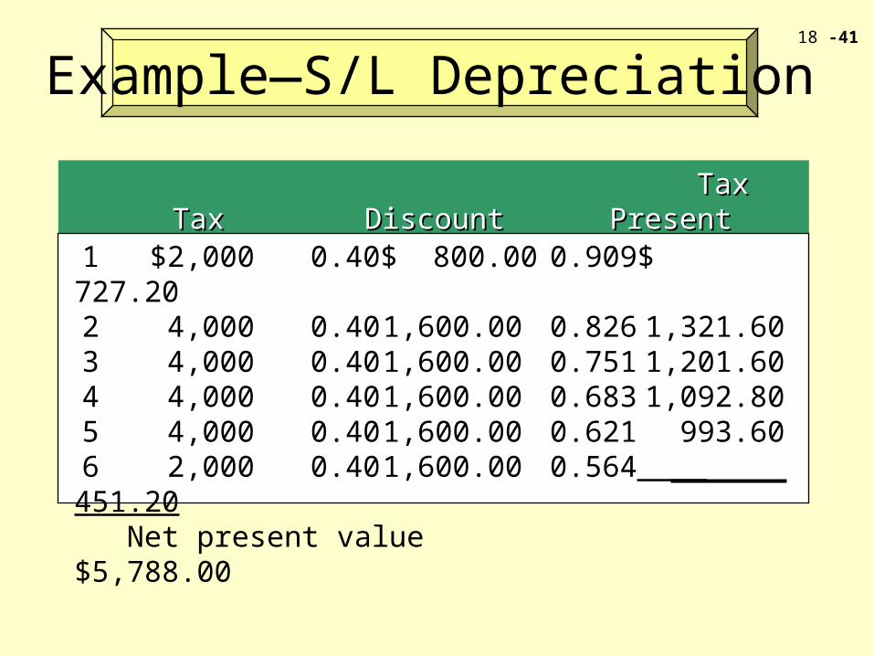
Example—S/L Depreciation

Tax Tax Discount PresentTax Tax Discount PresentYear Depreciation Rate Savings Factor ValueYear Depreciation Rate Savings Factor Value

1 $2,000 0.40 $ 800.00 0.909 $ 727.202 4,000 0.40 1,600.00 0.826 1,321.603 4,000 0.40 1,600.00 0.751 1,201.604 4,000 0.40 1,600.00 0.683 1,092.805 4,000 0.40 1,600.00 0.621 993.606 2,000 0.40 1,600.00 0.564 451.20

Net present value $5,788.00

18 -42

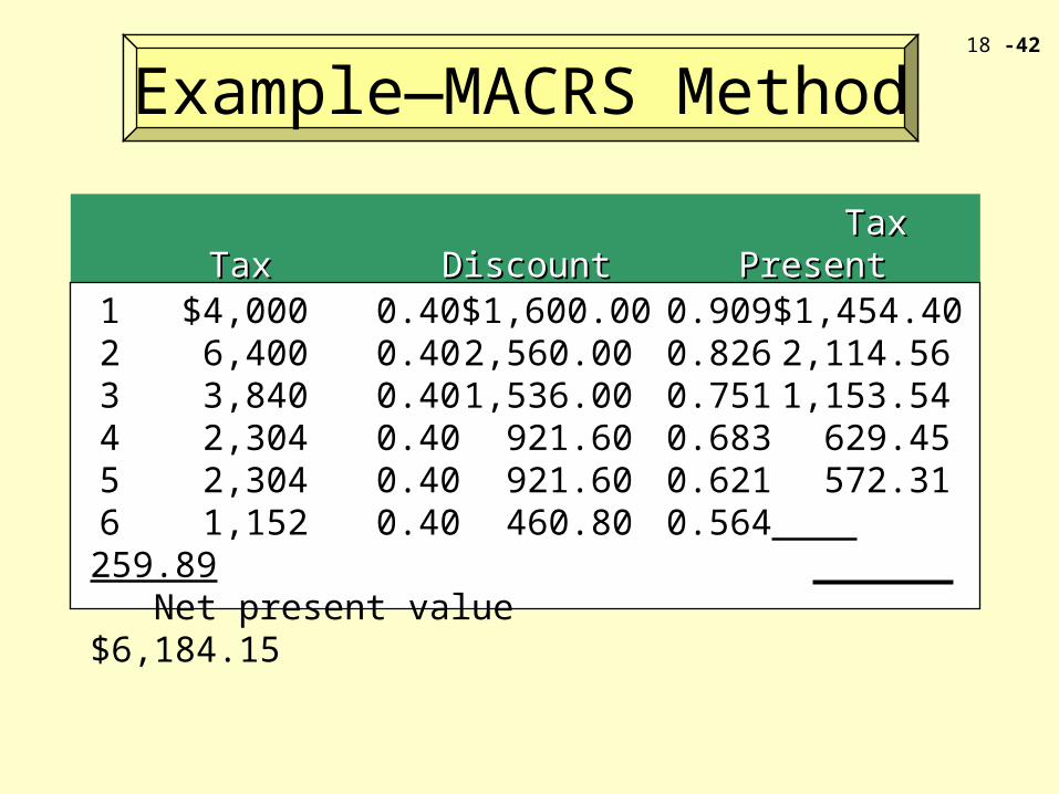
Example—MACRS Method

Tax Tax Discount PresentTax Tax Discount PresentYear Depreciation Rate Savings Factor ValueYear Depreciation Rate Savings Factor Value

1 $4,000 0.40 $1,600.00 0.909 $1,454.402 6,400 0.40 2,560.00 0.826 2,114.563 3,840 0.40 1,536.00 0.751 1,153.544 2,304 0.40 921.60 0.683 629.455 2,304 0.40 921.60 0.621 572.316 1,152 0.40 460.80 0.564 259.89

Net present value $6,184.15

18 -43

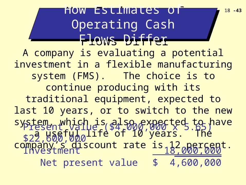
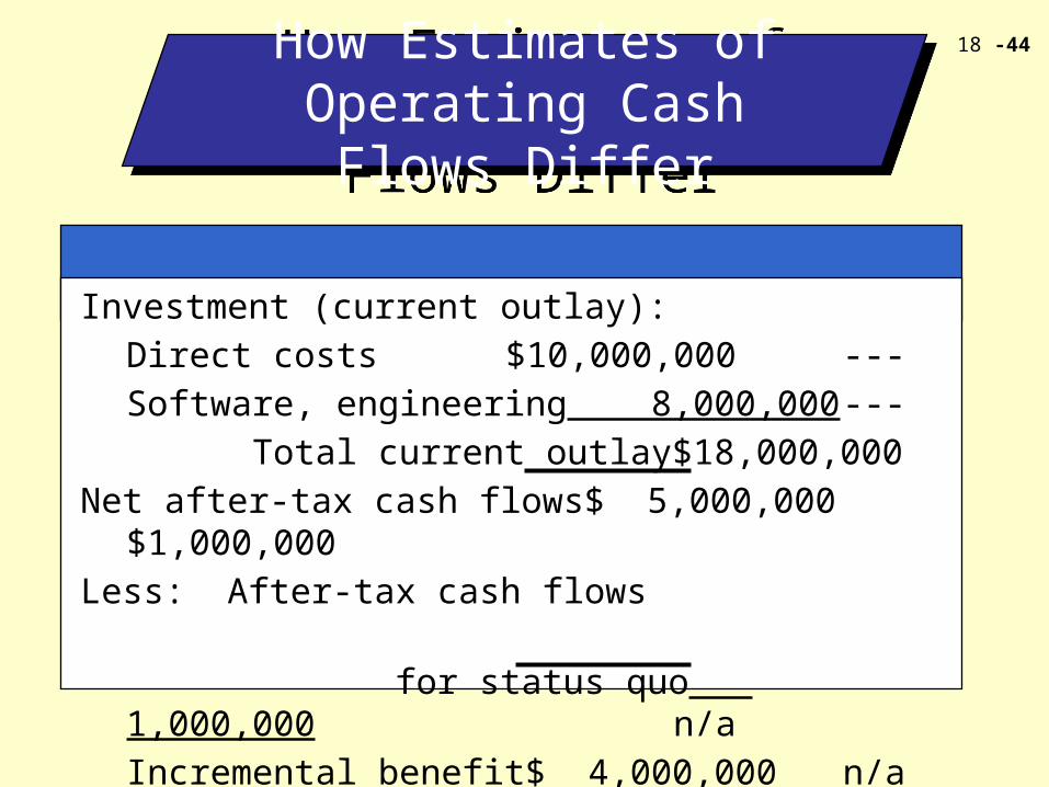
How Estimates of Operating Cash Flows Differ


A company is evaluating a potential investment in a flexible manufacturing system (FMS). The choice is to

continue producing with its traditional equipment, expected to last 10 years, or to switch to the new system, which is also expected to have a useful life of 10 years.

The company’s discount rate is 12 percent.

Present value ($4,000,000 x 5.65) $22,600,000Investment 18,000,000 Net present value $ 4,600,000

18 -44

FMS STATUS QUO FMS STATUS QUO

Investment (current outlay):

Direct costs $10,000,000 ---

Software, engineering 8,000,000 ---

Total current outlay $18,000,000

Net after-tax cash flows $ 5,000,000$1,000,000

Less: After-tax cash flows

for status quo 1,000,000 n/a

Incremental benefit $ 4,000,000 n/a



18 -45

INCREMENTAL BENEFIT EXPLAINEDINCREMENTAL BENEFIT EXPLAINED

Direct benefits:Direct labor $1,500,000Scrap reduction 500,000Setups 200,000

$2,200,000Intangible benefits (quality

savings):Rework $ 200,000Warranties 400,000Maintenance of competitive position 1,000,000

1,600,000Indirect benefits:

Production scheduling $ 110,000Payroll 90,000

200,000 Total

$4,000,000

FMS STATUS QUO FMS STATUS QUO

18 -46

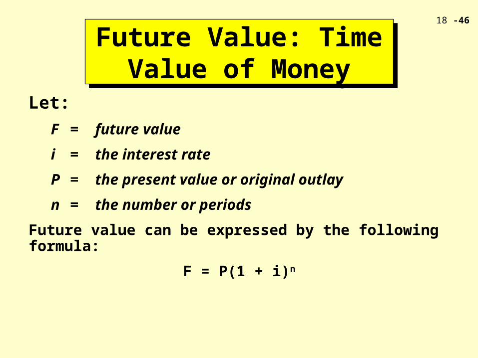
Future Value: Time Value of Money


Let:

F = future value

i = the interest rate

P = the present value or original outlay

n = the number or periods

Future value can be expressed by the following formula:

F = P(1 + i)n

18 -47

Assume the investment is $1,000. The interest rate is

8%. What is the future value if the money is

invested for one year? Two? Three?



18 -48

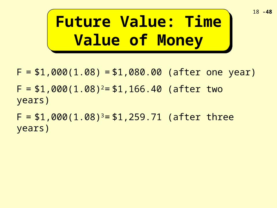
F = $1,000(1.08) = $1,080.00 (after one year)

F = $1,000(1.08)2 = $1,166.40 (after two years)

F = $1,000(1.08)3 = $1,259.71 (after three years)



18 -49

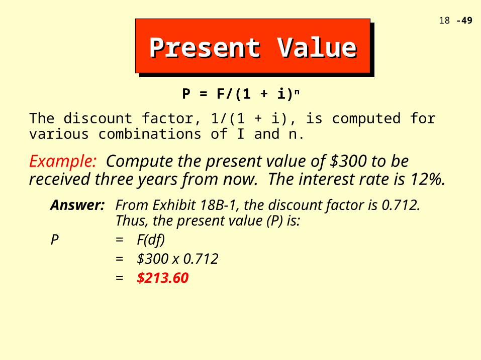
Present ValuePresent ValuePresent ValuePresent Value

P = F/(1 + i)n

The discount factor, 1/(1 + i), is computed for various combinations of I and n.

Example: Compute the present value of $300 to be received three years from now. The interest rate is 12%.

Answer: From Exhibit 18B-1, the discount factor is 0.712. Thus, the present value (P) is:

P = F(df)= $300 x 0.712= $213.60

18 -50

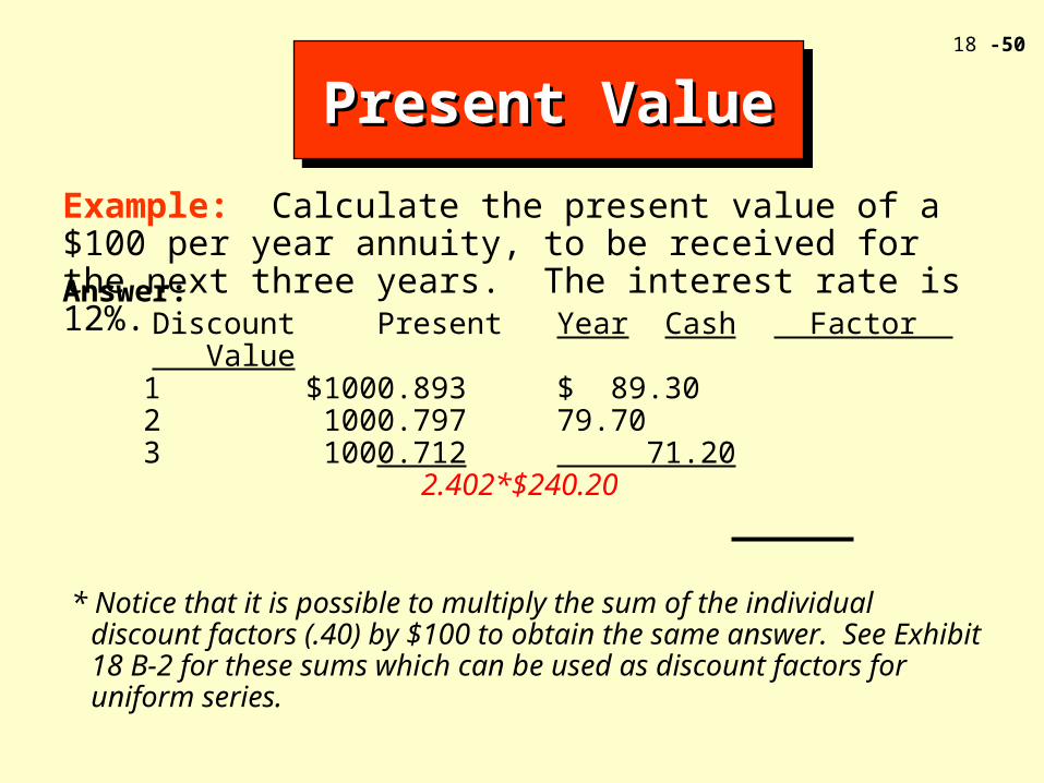
Answer:Discount Present Year

Cash Factor Value1 $100 0.893 $ 89.302 100 0.797 79.703 100 0.712 71.20

2.402* $240.20

Present ValuePresent ValuePresent ValuePresent Value

* Notice that it is possible to multiply the sum of the individual discount factors (.40) by $100 to obtain the same answer. See Exhibit 18 B-2 for these sums which can be used as discount factors for uniform series.

Example: Calculate the present value of a $100 per year annuity, to be received for the next three years. The interest rate is 12%.

18 -51

The EndThe EndThe EndThe End

Chapter EighteenChapter Eighteen

18 -52

Documents

Capital Investment Decisions