Impact of product pricing and timing of investment ... decisions as ﬁrms may not risk high investment in innovations due to the fear of opportunism by the other ﬁrm in setting

European Journal of Operational Research 180 (2007) 228–248

www.elsevier.com/locate/ejor

Production, Manufacturing and Logistics

Impact of product pricing and timing of investment decisionson supply chain co-opetition

Haresh Gurnani a,*, Murat Erkoc b, Yadong Luo a

a Department of Management, University of Miami, Coral Gables, FL 33124, United Statesb Department of Industrial Engineering, University of Miami, Coral Gables, FL 33124, United States

Received 17 October 2004; accepted 28 February 2006Available online 13 June 2006

Abstract

In supply chain co-opetition, firms simultaneously compete and co-operate in order to maximize their profits. We con-sider the nature of co-opetition between two firms: The product supplier invests in the technology to improve quality, andthe purchasing firm (buyer) invests in selling effort to develop the market for the product before uncertainty in demand isresolved. We consider three different decision making structures and discuss the optimal configuration from each firm’sperspective. In case 1, the supplier invests in product quality and sets the wholesale price for the product. The buyer thenexerts selling effort to develop the market and following demand potential realization, sets the resale price. In case 2, thesupplier invests in product quality followed by the buyer’s investment in selling effort. Then, after demand potential isobserved, the supplier sets the wholesale price and the buyer sets the resale price. Finally, in case 3, both firms simulta-neously invest in product quality and selling effort, respectively. Subsequently, observing the demand potential, the sup-plier sets the wholesale price and the buyer sets the resale price. We compare all configuration options from both theperspective of the supplier and the buyer, and show that the level of investment by the firms depends on the nature of com-petition between them and the level of uncertainty in demand. Our analysis reveals that although configuration 1 results inthe highest profits for the integrated channel, there is no clear dominating preference on system configuration from theperspective of both parties. The incentives of the co-opetition partners and the investment levels are mainly governedby the cost structure and the level of uncertainty in demand. We examine and discuss the relation between system param-eters and the incentives in desiging the supply contract structure.� 2006 Elsevier B.V. All rights reserved.

Keywords: Product pricing; Quality/technology investment; Supply chain design; Co-opetition; Game theory

1. Introduction

In supply chain co-opetition, firms may both compete and co-operate with each other in order to maximizetheir profits. Through co-operative relationships, the firms work to influence product demand by investing in

0377-2217/$ - see front matter � 2006 Elsevier B.V. All rights reserved.

doi:10.1016/j.ejor.2006.02.047

* Corresponding author. Tel.: +1 305 284 4712.E-mail addresses: [email protected] (H. Gurnani), [email protected] (M. Erkoc), [email protected] (Y. Luo).

mailto:[email protected]



H. Gurnani et al. / European Journal of Operational Research 180 (2007) 228–248 229

demand-enhancing efforts. These efforts may include, for example, investment in technology by one firm toimprove product quality/design, as well as investment in selling effort by the other firm to develop the marketfor the product. The cost of these selling effort is incurred by the firm that exerts effort but the benefit, in formof improved demand potential, affects both firms. As such, due to the spillover effect, investment in innovationby either firm can benefit both supply chain partners. For instance, in the personal computer industry, demandfor computers depends not only on the investment by Intel in newer generation of faster processors, but alsoon the innovations from the computer manufacturers (for e.g. Dell) in investing in infrastructure to providecustomer support services. At the same time, the firms independently set prices in order to maximize theirprofits: the firm investing in product technology (supplier) may prefer to charge a higher wholesale price tothe buying firm (buyer), whereas the firm exerting selling effort to develop the market (buyer) may prefer ahigher resale price in the end-market. The timing of the price commitment decisions can influence the invest-ment decisions as firms may not risk high investment in innovations due to the fear of opportunism by theother firm in setting a high price. We analyze the nature of both product pricing and timing of investmentdecisions for the two firms depending on the structure of the contract between them.

In this paper, we consider the problem of supply contract design for a one-time interaction between a sup-plier and a buyer. This assumption is widely used in the supply chain contracting literature and is applicable tomany settings including those with seasonal or high-tech products. The main purpose and motivation of usingsuch approach is to derive managerial insights for high level managers in supply chains. We study the problemat a macro level in order to investigate the incentives and equilibrium investment policies in a two echelonsupply chain, and the contribution of the paper is to study the effect of timing of price commitment decisionson the investment decisions and on the profits for the two firms. While both the firms can benefit from eachother’s investment in product quality and selling effort, respectively, the timing of the price commitment deci-sions influences the level of investment by the firms. As such, the nature of competition between firms affectsthe level of co-operation they provide to each other.

The supplier invests in the technology used to make the product; a larger investment in technology improvesthe quality of the product which results later in an increased demand potential for the product. However, thetechnology investment/quality-improvement costs are directly incurred by the supplying firm only. As such, thesupplier may charge a high wholesale price in order to recuperate these costs. For instance, in the electricitymarkets, power generating firms can invest in different dimensions of power quality such as environmen-tally-friendly green power or premium power for sensitive computing, as opposed to lower quality interruptiblepower for flexible producers (Savitski, 2002). In the fast food retail business, final demand is not only affected bythe retail price and the value added by the buyer, it also depends on the investments made by the franchisor inits brand name (Lal, 1990). In the automotive industry, Japanese firms made dramatic gains in market share inthe 1980s as compared to the US firms by investing in quality-improvement efforts (Garvin, 1988).

Similarly, the buyer, e.g., a retailer, has the opportunity to influence final demand by choosing the appro-priate selling/promotional efforts. Examples of such activities include breaking bulk, providing shelf spaces,promotional displays, advertising, and other demand enhancing activities. In the automotive industry, finaldemand depends not only on the quality/brand reputation of the product, but also on the dealer’s sellingefforts including customer financing and after-sales service support, etc. The cost of these promotional effortsis directly incurred by the dealer only.

In general, demand enhancing investments such as the supplier’s technology choice and the buyer’s marketbuilding efforts involve long lead times and often need to be committed before final demand information forthe end product is revealed. Therefore, in our setting, such investments are committed before demand uncer-tainty is resolved. On the other hand pricing decisions, i.e., the supplier’s wholesale pricing and the buyer’sresale pricing, can be postponed until after final demand potential is observed. While both firms can investin demand enhancing innovations, there is a possibility that they may under-invest due to the fear that theother firm may take advantage of improved demand potential by charging a high price. As such, the invest-ment and pricing decisions are inter-linked and the timing of price commitment would influence the level ofinvestment in demand enhancing innovations. In order to analyze this, we model the structure of the decisionmaking process between a supplier, S, selling a product through an independent buyer, B.

We consider three possible cases as outlined in Fig. 1: In case 1, the supplier invests in technology and offersthe product with a certain quality and wholesale price to firm B. There is no negotiation over the contract

230 H. Gurnani et al. / European Journal of Operational Research 180 (2007) 228–248

terms – Firm B may accept the contract or reject it, in which case both sides could walk away. If firm B decidesto accept the contract, he can influence the demand through his promotional/selling efforts. He determines theoptimal selling effort before observing the final demand potential and postpones his resale pricing decisionsuntil after uncertainty is resolved. Here, except for demand uncertainty, there is no source of risk for firmB since firm S commits to both wholesale price and quality-investment decisions a priori; In case 2, the sup-plier first invests in the technology and sets the product quality; subsequently, firm B invests in selling effort inorder to develop the market. Here, both firms make their investment decisions sequentially without makingany price commitments. Then, followed by the realization of the final demand potential, the supplier setsthe wholesale price, and finally, firm B sets the optimal resale price. Here, firm B faces a higher risk sincehe makes his investment decision prior to the wholesale price commitment from firm S; In case 3, the supplierand buyer simultaneously invest to set the product quality and the selling effort, respectively. Again, the invest-ment decisions are made prior to any price commitment, but now, both firms simultaneously make these deci-sions. Then, similar to case 2 above, demand uncertainty is resolved, the supplier sets the wholesale price, andfinally the buyer determines the optimal resale price.

In the comparison of the three cases, we discuss the role of uncertainty, cost of building quality, and thecost of selling effort in determining the preference for a certain decision-making configuration. We show thatthere is no clear dominating preference on system configuration for both parties – The preferences of the co-opetition partners and the investment levels are mainly governed by the investment costs and the level ofdemand uncertainty. Our analysis indicates that if wholesale price is not committed by the supplier beforethe market is developed, the buyer will always under invest in his selling effort. This result is mainly due tothe fear of supplier opportunism. Clearly, in such cases, the supplier can benefit from the buyer’s selling effortby charging a high wholesale price. It turns out that low investment in selling effort by the buyer eventuallyhurts the supplier’s profits, and the system as a whole. Consequently, we observe that the supplier prefers to bethe leader and make her pricing and quality investment decisions first when demand uncertainty is low. On theother hand, if cost of selling effort is low, the buyer expects the supplier to free ride on his selling effort andhence prefers that the supplier commit to the wholesale price first. Based on this observation, we show thatwhen investment costs are sufficiently low, both parties prefer configuration 1, which also yields the highestintegrated channel profits.

However, we observe that the level of demand uncertainty and investment costs can lead to conflicting pref-erences for the co-opetition partners when investment costs are high. When demand variability is high, theincreased value of information motivates the supplier to give up some of her first-mover advantage in returnfor postponement of her pricing decision. In this case, the supplier would prefer configuration 2. On the otherhand, while intuition suggests that the buyer would always prefer to make his investment decision after the sup-plier has set the wholesale price, under certain conditions, it may be optimal for the buyer to simultaneouslymake investment decisions along with the supplier even though no wholesale price commitment has been made.We show that if cost of selling effort is high, the buyer would benefit from the supplier’s investment in quality incase 3 and profits would be higher in case 3 even without the wholesale price commitment from the supplier.Here the supplier invests more in product quality in case 3 as compared to case 1, and therefore, the profitsfor the buyer may be higher since his investment in selling effort will be lower compared to case 1.

The rest of the paper is organized as follows. In Section 2, we discuss the related concepts and examples,and discuss some related literature. In Section 3, we formulate the model and determine the optimal expres-sions for various decision making structures. In Section 4, we compare the different configurations and discusseach firm’s preference for a certain decision-making structure. Finally, we conclude the paper in Section 5.

2. Related concepts and examples

Co-opetition refers to the interdependence in which competition and co-operation occurs between two ormore firms. It looks for win-win scenarios in which firms strive to increase the size of the total pie which theycan divide up (Luo, 2004). The interdependence entails competing and collaborating elements, with rivalry aswell as collaborative mechanisms, in course of maximizing individual profits (Brandenburger and Nalebuff,1996). Co-operative elements can nourish joint payoff creation through exploiting complementary resourcescooperatively. Meanwhile, competitive elements can breed conflicts that may emerge when either party


emphasizes its own gains from specific projects or transactions in which respective needs are not compatible.Competitive aims always exist because of the underlying incentive for any party to share a higher percentageof returns generated from co-operation. The simultaneity of co-operation and competition arises because firmshave both private goals and common goals as they deal with other businesses such as suppliers or buyers.

Co-opetition is mainly attributed to increasing interdependence between firms (e.g., wholesaler versus retai-ler or buyer versus supplier) and heightened needs for collective actions, risk sharing, strategic flexibility, jointreturn enhancement, and prompt response to market demands. Co-opetition implies the existence of co-oper-ation and competition between the same firms, not about co-operation with one firm and competing withanother firm. The latter, also an important issue and prominent phenomenon in building cooperative alliances,has been addressed in several studies such as Lado et al. (1997), Dyer and Singh (1998) and Gnyawali andMadhavan (2001). Co-operation and competition between the same firms are attributed to increasing interde-pendence between global players and heightened needs for collective actions, risk sharing, strategic flexibility,and prompt response to market demands.

In the operations literature, researchers have focused on supply chain coordination by designing incentivemechanisms such that all members in the supply chain align their objectives with the system-wide objective,that is, to achieve channel coordination. A variety of mechanisms have been studied to improve supply chainefficiency including buy-back agreements (Pasternack, 1985), quantity commitment contracts (Anupindi andBassok, 1999), and information sharing (Gavirneni et al., 1999). However, the operations literature has notstudied co-opetitive investment interactions among firms in a supply chain. In a paper in the economics/indus-trial organization area, Klein et al. (1978) discuss how and when relation-specific investments can lead toopportunistic behavior among vertically related firms. However, their paper focuses on conditions when ver-tical integration is preferred to decentralization. Finally, in a paper in the marketing literature, Amaldoss et al.(2000) examine how resource commitments by alliance partners is influenced by three structural variables: theprofit-sharing arrangement between the firms, the type of alliance as modeled by the rule for combining part-ners’ inputs, and the size of the market reward for winning the inter-alliance competition.

The objective of our study is to focus on different types of decision-making structures. As such, we study thevarious sequences used by the firms in making both investment and pricing decisions in the supply chain. Weare able to show the preference of the supplier and the buyer for certain configurations, depending on the costof building quality as well as the cost of selling effort. To the best of our knowledge, there is no similar study ofthe contract selection problem when both the buyer and the supplier can use price and non-price factors to co-operate and compete with each other in the supply chain.

There are many examples that fit well into one or more of the cases that we study in the paper. In thisregard, we believe that the models studied in this paper and insights generated therefrom have not only the-oretical importance but also practical appeal.

For example, in a scenario based on case 1, Lowe’s, the second-largest home improvement retailer in theworld, buys toilet products from one of dozen vendors including Fluidmaster, based in San Juan Capistrano,CA, (Kern, 2002). Vendors such as Fluidmaster constantly invest to improve the product quality or to includenovel features. In the vendor agreement, Fluidmaster sets its wholesale price for various product types, andLowe specifies its expectations in various areas such as on-time shipment, quantity fill rate, bar coding, pack-aging requirements, and other policies with which all vendors must comply. There is no negotiation over theseterms or requirements. With this pre-documented standardized agreement, Fluidmaster, like some other ven-dors, can either accept or reject the contract with Lowe. If these conditions are not acceptable, Fluidmastermay approach Home Depot which is also the company’s main buyer. Likewise, Lowe can accept or rejectFluidmaster’s offer since it has many other vendors available to ship toilet parts. If Lowe signs a vendor agree-ment, it will then decide the retail price as well as the selling efforts (more promotional efforts are made towardhigh price-point goods or brand products), (Canlen, 2002).

In an example based on case 2 scenario, Cepheid Corporation, based in Sunnyvale, CA, is a leading devel-oper and manufacturer of miniaturized, fully integrated systems of rapid detection of DNA, the universal bio-logical identifier. The Smart Cycler System (SCS), its flagship product, amplifies and analyzes DNA for lifescience research faster than other analyzers. In 2002, Cepheid signed a multi-year distribution agreement withIzasa SA based in Barcelona, Spain, to market the Cepheid SCS in Spain, Portugal, Italy, Austria, France, theNetherlands and the United Kingdom. To reap benefits from high profit margin in this product/market


segment, both firms decided to put more investments in respective areas: Cepheid invests in technology anddevelopment and sequentially, Izasa invests in marketing and sales in order to create a win-win payoff. Accord-ing to the agreement, Izasa provides marketing, sales and service support for Cepheid’s SCS, and such market-ing plans (including advertising investments and resale pricing) are sequentially linked to Cepheid’s precedinginvestments in innovation, customization, and product quality. For instance, for better-innovated and custom-ized SCS’s manufactured by Cepheid, Izasa will invest more in marketing and promotion, in the use of CH-Werfen, a network of sales and marketing of health care products in Europe, (Anonymous, 2002). Izasa setsthe resale price on the basis of its purchasing costs (i.e., Cepheid’s wholesale price), the actual investments inmarketing and promotion, as well as market demand conditions it has influenced through advertising.

The next example exemplifies the third case scenario. Guidant Corporation, a world leader in the design anddevelopment of cardiovascular medical products has a distribution agreement with Henry Schein Inc., anational distributor of medical supplies, (Burton, 1998). Guidant (the supplier) and Henry Schein (distributor)simultaneously invested to develop cutting-edge products and marketing and promotion, respectively. Guidantinvested enormously in the multi-link pixel coronary stent, which provides physicians with an immediate, min-imally invasive way of treating blockages in small diameter vessels, while Henry Schein simultaneouslylaunched a new promotional effort, through catalogs, trade shows, and advertisement, to enhance nationwidesales of coronary stent. Because the resale price was determined solely by Henry Schein (the original wholesaleprice was set by Guidant), the distributor was motivated to marketing so as to profit from higher margin.

In business practice, all three channel structures can exist as discussed above. However, the selection of anappropriate channel structure would depend on a number of factors including the presence of other compet-itors, demand uncertainty, information asymmetry, sequence of product pricing commitment/investment deci-sions, etc. In this paper, we focus on the role of sequence of product pricing commitment decisions on theinvestment decisions and on the overall profits for the firms.

3. Model formulation

We define the following notation. Let h be the quality level selected by the supplier and x be the wholesaleprice charged to the buyer. The buyer’s selling effort is e, and the resale price set in the end-market is p. With-out loss of generality, we normalize the retail demand expression, D to be:

D ¼ a� p þ ceþ khþ n;

where a is the market size, n is the error term on demand with mean 0 and standard deviation r, c measures theinfluence of buyer’s selling effort on demand, and k measures the impact of product quality on demand. Sim-ilar demand models have been used in the marketing literature by Desai and Srinivasan (1995) and Desai(1997). We do not assume any specific distribution for n but note that the lower support is such that the de-mand is always non-negative. Since the resale pricing decision is made after realization of demand uncertainty,if the realized outcome is very low and demand is likely to be negative at the lowest possible resale price, therewould be no transaction between the buyer and the supplier.

3.1. Case 1: Product quality and price commitment by supplier

In the first case (see Fig. 1A), the supplier acts as the leader and determines the investment in product qual-ity/design and sets the wholesale price for the buyer prior to the realization of n. Subsequently, the buyerdetermines the optimal selling effort and after observing n, the resale price.

In the analysis of this model, we determine the optimal decisions in the two stages of the problem. First, wedetermine the optimal resale price for the buyer for a given contract (x, h) offered by the supplier and e

decided by the buyer before the realization of n. Then, we find the optimal selling effort that maximizes theexpected buyer profit. Next, we determine the optimal contract offered by the supplier given the best responseof the buyer. After the realization of n, the buyer’s objective function is

MaxðpÞ½PBðpÞ ¼ ðp � xÞ½a� p þ ceþ khþ n� � ge2=2�;

Uncertainty in demand is resolved (ξ)

Buyer sets resale price (e, p)

Buyer invests in developing the market (e)

Supplier invests in product quality andsets wholesale price (θ,ω)

Fig. 1A. Case 1 – product quality and price commitment by supplier.


where the cost of selling effort is assumed to be ge2/2. Similar to the existing marketing literature, we use con-vex cost of investment to model the diminishing return of investment in influencing demand. It is easy to seethat the buyer’s profit function is concave in p. Then, from the first order conditions, we have:

oPB

op¼ 0) p ¼ aþ ceþ khþ xþ n

2:

Using the expression of p from above, we can re-write the expected profit of the buyer as follows:

E½PB� ¼aþ ceþ kh� x

2

� �2

þ r2

4� ge2

2: ð1Þ

Next, we find the optimal selling effort level that maximizes the buyer’s expected profit:

oE½PB�oe

¼ 0) e� ¼ c2g� c2

ðaþ kh� xÞ: ð2Þ

In order to ensure concavity and that there are no pathological cases of negative selling effort, we require that2g > c2. Thus, using e* from (2) we get:

p� ¼ ðaþ khÞgþ ðg� c2Þxð2g� c2Þ þ n

2: ð3Þ

Define K ¼ gð2g�c2Þ. On substituting from above in (1) and simplifying terms, we get:

E½P�Bðx; hÞ� ¼K2ðaþ kh� xÞ2 þ r2

4; ð4Þ

and Dðx; hÞ ¼ a� p þ ceþ khþ n

¼ Kðaþ kh� xÞ þ n2: ð5Þ

The supplier invests in quality improvement efforts that may include new high-precision equipment with highreliability, fast or flexible equipment, organizational training and restructuring, etc., which improve the de-mand potential of the product. Another example of supplier-initiated effort to improve the demand potentialis the investment in brand name (see Lal, 1990). By inferring the buyer’s selling effort reaction function in re-sponse to the terms of the contract, the supplier can suitably choose the contract in order to maximize hisprofits.

The quality level selected by the supplier h, affects his total expected costs in two ways: First, investment inquality improvement programs increases fixed costs, fh2/2. The quality level also has an impact on the variable


costs. We let the variable costs be c(1 + vh), where v may be less than or greater than zero. Allowing v to benegative allows us to model the case when the variable production costs actually decline due to improvementin quality (Banker et al., 1998). Then, we get:

1 We

Maxðx;hÞ

E½PS � ¼ E ðx� cð1þ vhÞÞD� fh2

2

� �� ;¼ E ðx� cð1þ vhÞÞ Kðaþ kh� xÞ þ n

2

� �� fh2

2

� �: ð6Þ

We can show that the supplier’s profit function is concave as the Hessian is negative semi-definite if(2f � K(k � cv)2) > 0. We shall assume that the above condition is valid. Then, from the first order conditionsand noting that E[n] = 0, we get:

oE½PS �ox

¼ 0) x ¼ aþ khþ cð1þ vhÞ2

; ð7Þ

andoE½PS �

oh¼ 0) h ¼ Kðkðx� cÞ � cvða� xÞ � kcÞ

ð2kKcvþ fÞ : ð8Þ

Solving (7) and (8) for x and h, we get:1

x�1 ¼fðaþ cÞ þ Kcðk� cvÞðav� kÞ

ð2f� Kðk� cvÞ2Þ; ð9Þ

and h�1 ¼Kðk� cvÞða� cÞð2f� Kðk� cvÞ2Þ

: ð10Þ

Substituting into (6) and upon simplifying terms, we get:

E½P�S1� ¼fKða� cÞ2

2ð2f� Kðk� cvÞ2Þ: ð11Þ

From (2)–(5), we get:

p�1 ¼ x�1 þfKða� cÞ

ð2f� Kðk� cvÞ2Þþ n

2; ð12Þ

e�1 ¼cfKða� cÞ

gð2f� Kðk� cvÞ2Þ; ð13Þ

D�1 ¼fKða� cÞ

ð2f� Kðk� cvÞ2Þþ n

2; ð14Þ

and E½P�B1� ¼K2

fða� cÞð2f� Kðk� cvÞ2Þ

!2

þ r2

4: ð15Þ

We note from above that h�1, p�1, e�1 and E½P�S1�, E½P�B1� are decreasing in c, as expected. Further, observe thatthe optimal terms of the contract offered by the supplier depend on the buyer’s cost of selling effort, g. We canshow that (h�1, x�1) and (p�1, e�1) are all decreasing in g, as expected. That is, if the buyer has a lower cost ofselling effort, he is likely to provide more effort, and in anticipation of the same, the supplier provides a higher

quality product. As such, both the wholesale price and the resale price are also higher. Also, note thatoP�S1

og ,oP�B1

og < 0, andoP�S1

of ,oP�B1

of < 0, that is, the suppliers’ and buyer’s profits are decreasing in increasing cost of sellingeffort and in the cost of building quality. We observe from (11) and (15) that while expected supplier profits areindependent of level of uncertainty in demand, expected buyer profits increase in r.

use the subscript ‘1’ to denote the optimal expressions for the contract problem in case 1.


3.2. Case 2: Product quality commitment by supplier

In case 2 (see Fig. 1B), the supplier first determines the investment in product quality/design and the buyerthen invests in selling effort to develop the market. Here, both players make their investment decisions prior toany wholesale price commitment by the supplier and realization of n. Pricing decisions are postponed untilafter n is observed. Then, the supplier sets the wholesale price, and finally, the buyer determines the optimalresale price.

Unlike the three-stage analysis in case 1, here we have four stages to consider: We first solve the last stageproblem to determine the optimal resale price as a function of the other three decisions. Next, we determinethe solution to stage 3 where the supplier determines the optimal wholesale price given the decisions made instages 1 and 2, and recognizing the optimal reaction function of the buyer in setting the resale price in stage 4.Then, we solve the stage 2 problem where the buyer determines the optimal selling effort, and finally, we solvethe stage 1 problem where the supplier determines the optimal investment in product quality/design.

The buyer’s objective in stage 4 is to determine the optimal resale price, that is

MaxðpÞ½PBðpÞ ¼ ðp � xÞ½a� p þ ceþ khþ n� � ge2=2�; ð16Þ

which yields p� ¼ ðaþ ceþ khþ xþ nÞ2

; ð17Þ

and D� ¼ ðaþ ceþ kh� xþ nÞ2

: ð18Þ

The supplier’s objective in stage 3 is to determine the optimal wholesale price, that is

MaxðxÞ½PSðxÞ ¼ ðx� cð1þ vhÞÞ aþ ceþ kh� xþ n

2

� �� fh2=2�; ð19Þ

which yields x� ¼ ðaþ ceþ khþ cð1þ vhÞ þ nÞ2

: ð20Þ

In stage 2, n is not observed yet. The buyer’s objective in stage 2 is to determine the optimal selling effort, thatis

MaxðeÞ

E½PBðeÞ� ¼aþ ceþ kh� cð1þ vhÞ

4

� �2

þ r2

16� ge2

2

" #; ð21Þ

Buyer invests in developing the market (e)

Supplier invests in product quality (θ)

Supplier sets wholesale price (ω)

Buyer sets resale price (p)


Fig. 1B. Case 2 – product quality commitment by supplier.


which yields e� ¼ c8g� c2

aþ kh� cð1þ vhÞð Þ: ð22Þ

Finally, the supplier’s objective in stage 1 is to determine the optimal investment in product quality/design,that is

MaxðhÞ

E½PSðhÞ� ¼8g2

ð8g� c2Þ2aþ kh� cð1þ vhÞ½ �2 þ r2

8� fh2

2

" #; ð23Þ

which yields h�2 ¼K2

2ðk� cvÞða� cÞf� K2

2ðk� cvÞ2: ð24Þ

where, K2 ¼ 4g8g�c2. We note that since K > 2K2

2, our assumption of (2f � K(k � cv)2) > 0 (in case 1) also ensures

concavity in this case. Substituting backwards into (22), (20) and (17), we get:

e�2 ¼cfK2ða� cÞ

4gðf� K22ðk� cvÞ2Þ

; ð25Þ

x�2 ¼K2fða� cÞ

f� K22ðk� cvÞ2

þ cf� K2

2ðk� cvÞðk� avÞðf� K2

2ðk� cvÞ2Þþ n

2; ð26Þ

p�2 ¼ x�2 þfK2ða� cÞ

2ðf� K22ðk� cvÞ2Þ

þ n4; ð27Þ

D�2 ¼fK2ða� cÞ


þ n4; ð28Þ

and E½P�S2� ¼fK2

2ða� cÞ2


þ r2

8; ð29Þ

E½P�B2� ¼K2

8

fða� cÞðf� K2

2ðk� cvÞ2Þ

" #2

þ r2

16: ð30Þ

Again, similar to the result in case 1, we can show thatoP�S2

og ,oP�B2

og < 0, andoP�S2

of ,oP�B2

of < 0, that is, the suppliers’and buyer’s profits are decreasing in increasing cost of selling effort and in the cost of building quality. In con-trast to the previous case, the supplier’s expected profits depend on the level of demand uncertainty since shenow postpones her pricing decision in this scenario. In fact, both players’ profits increase in r, though, theexpected buyer profits are less sensitive to demand uncertainty compared to the previous case.

3.3. Case 3: Simultaneous product quality commitment by supplier and selling effort commitment by buyer

In case 3 (see Fig. 1C), the supplier and buyer simultaneously determine the investment in product designand selling effort, respectively. Then, n is realized, the supplier sets the wholesale price, and finally, the buyerdetermines the optimal resale price.

Here we have three stages to consider: We first solve the last stage problem to determine the optimal resaleprice as a function of the other three decisions. Next, we determine the solution to stage 2 where the supplierdetermines the optimal wholesale price given the decisions made in stage 1 and the optimal reaction functionof the buyer in stage 3. Finally, we solve the stage 1 problem where the supplier and the buyer move simul-taneously and determine the optimal investment in product quality/design and selling effort, respectively. Thebuyer’s objective in stage 3 is to determine the optimal resale price, that is

MaxðpÞ½PBðpÞ ¼ ðp � xÞ½a� p þ ceþ khþ n� � ge2=2�; ð31Þ

which yields p� ¼ ðaþ ceþ khþ xþ nÞ2

: ð32Þ

Supplier invests in product quality and Buyer invests in developing the market

(θ, e)

Supplier sets wholesale price (ω)

Buyer sets resale price (p)


Fig. 1C. Case 3 – simultaneous investments by buyer and supplier.


The supplier’s objective in stage 2 is to determine the optimal wholesale price, that is

MaxðxÞ½PSðxÞ ¼ ðx� cð1þ vhÞÞ aþ ceþ kh� xþ n

2

� �� fh2=2�; ð33Þ

which yields x� ¼ ðaþ ceþ khþ cð1þ vhÞ þ nÞ2

: ð34Þ

The stage 1 problem is to simultaneously determine the optimal investment in product quality/design and theselling effort. For the buyer, the objective is

MaxðeÞ

E½PBðeÞ� ¼aþ ceþ kh� cð1þ vhÞ

4

� �2

þ r2

16� ge2

2

" #; ð35Þ

and, for the supplier, the objective is

MaxðhÞ

E½PSðhÞ� ¼aþ ceþ kh� cð1þ vhÞ½ �2

8þ r2

8� fh2

2

" #: ð36Þ

In order to ensure concavity and that there are no pathological cases of negative selling effort or product qual-ity, we require that (f � K3(k � cv)2) > 0, where K3 ¼ 2g

4g�c2. Solving (35) and (36) simultaneously for h and e,we get:

h�3 ¼K3ðk� cvÞða� cÞf� K3ðk� cvÞ2

; ð37Þ

and e�3 ¼cfK2ða� cÞ

4gðf� K3ðk� cvÞ2Þ: ð38Þ

Theorem 3.1. Assume that (f � K3(k � cv)2) > 0. Then, there is a unique Nash equilibrium to the simultaneous

game between the buyer and the supplier in case 3.

Proof. All Proofs are in the Appendix.

Substituting (37) and (38) backwards into (34) and (32), we get:

x�3 ¼ cþ ða� cÞK2fþ K3ðk� cvÞcv

f� K3ðk� cvÞ2þ n

2; ð39Þ

TableResult

Qualit

Selling

Suppli

Buyer

Chann


p�3 ¼ x�3 þfK2ða� cÞ

2ðf� K3ðk� cvÞ2Þþ n

4; ð40Þ

D�3 ¼fK2ða� cÞ

2ðf� K3ðk� cvÞ2Þþ n

4; ð41Þ

and E½P�S3� ¼ ðfK22 � K2

3ðk� cvÞ2Þ fða� cÞ2

2ðf� K3ðk� cvÞ2Þ2þ r2

8; ð42Þ

E½P�B3� ¼K2

8

fða� cÞðf� K3ðk� cvÞ2Þ

" #2

þ r2

16: ð43Þ

Similar to the result in cases 1 and 2, we can show thatoE½P�S3

�og ,

oE½P�B3�

og < 0, that is, the suppliers’ and buyer’sprofits are decreasing in increasing cost of selling effort. However the effect of cost of quality is different. While

we note thatoE½P�B3

�of < 0, we have

oE½P�S3�

of > 0, that is, while the buyer’s profits are decreasing in increasing cost ofquality, the supplier’s profits are increasing in the cost of quality. Essentially as cost of quality increases, thesupplier reduces her investment in quality and instead is able to free ride on the buyer’s investment in sellingeffort. Hence, counter to our expectation, the supplier actually benefits if the cost of quality is high. However,

for the system as a whole,oðE½P�S3

�þE½P�B3�Þ

of < 0, that is, profits for the system are decreasing with increasing cost ofquality, as expected. We note that a similar effect is not observed for an increase in cost of selling effort. Here,the buyer is not able to free ride on the supplier’s investment in quality since the supplier has the ability tonegate this by charging a higher wholesale price later. Hence, the profits for both firms are decreasing asthe cost of selling effort increases, as expected. The impact of demand uncertainty on players’ expected profitsare similar to case 2.

4. Channel configuration comparisons

In the previous section, we derived the expressions for the optimal parameters for the three cases. In thissection, we compare the configurations and discuss the potential of conflicting choices between the buyer andthe supplier.

4.1. Two-way comparisons

We first compare configuration pairs from the perspective of the supplier, the buyer, and the integratedchannel. The results are summarized in Table 1 and discussed below. Later, we discuss the results of thethree-way comparison.

1s of two-way comparisons

Cases 1 and 2 Cases 2 and 3 Cases 1 and 3

y investment h�1 > h�2 h�2 < h�3 h�1 > h�3 if c2 < 2g < 3c2/2;h�1 < h�3 if 2g > 3c2/2.

effort investment e�1 > e�2 e�2 < e�3 e�1 > e�3

er profits E½P�S1� > E½P�S2� for lowdemand variability

E½P�S2� < E½P�S3� E½P�S1� > E½P�S3� for lowdemand variability

E½P�S1� < E½P�S2� for highdemand variability

E½P�S1� < E½P�S2� for highdemand variability

profits E½P�B1� > E½P�B2� E½P�B2� < E½P�B3� E½P�B3� < E½P�B3� for lowdemand variabilityE½P�B1� < E½P�B3� for highdemand variability

el profits E½P�S1� þ E½P�B1� > E½P�S2� þ E½P�B2� E½P�S2� þ E½P�B2� > E½P�S3� þ E½P�B3� E½P�S1� þ E½P�B1� > E½P�S3� þ E½P�B3�


4.1.1. Comparison of case 1 and case 2 configurations

In case 1, the supplier announces both the quality investment and the wholesale price before the buyer com-mits to anything and all supplier decisions are to be made before the realization of demand uncertainty. Thetrade-off for the supplier is to enjoy the first-mover advantage associated with the leadership position or topostpone decisions until after demand uncertainty is resolved.

Lemma 1. (a) When product quality/design investment and wholesale price commitment is initially made by the

supplier, the supplier invests more in product quality, and the buyer invests more in selling effort, that is, h�1 > h�2and e�1 > e�2.

(b) The buyer prefers that the supplier commit to both product quality/design and wholesale price decisions

before all buyer commitments, that is, E½P�B1� > E½P�B2�. The integrated channel as a whole is also better off in

case 1. However, the supplier is better off by postponing the wholesale price decision and thus, prefers case 2 over

case 1 if and only if r is beyond a certain threshold.

It can be observed from (3) and (12) that the buyer’s resale price is higher in the first case unless n turns outto be negative and sufficiently small. In general the buyer will tend to charge more in case 1 as it makes higherinvestment in selling effort. However, the resale price in case 1 is more sensitive to the realization of n, as it isthe only means that is used to adjust to variations in demand as opposed to case 2 where wholesale price is alsopostponed until the uncertainty is resolved. As such, if the realized value of n is too small the buyer will becompelled to offer larger price cuts in case 1 and hence may end up charging a lower resale price. We also notethat the wholesale price charged by the supplier in case 1 is not necessarily higher than the price charged incase 2 even though h�1 is greater than h�2. In fact, for a given n, there exists a threshold of f (the cost of buildingquality), such that, w1 < w2 if f exceeds this critical threshold. In general for low cost of quality, w1 > w2. Theintuition for this observation is as follows: As f increases, even though h�1 > h�2, the supplier’s investment inquality decreases and the difference in quality investment between the two cases is smaller. As such, the com-parative role of product quality in influencing demand is diminished.

In case 2, the buyer makes the investment in selling effort after the supplier has invested in product qual-ity/design, but before the wholesale price is set. As such, the buyer has the risk of over investing in devel-oping the market and facing a high wholesale price from the supplier. Therefore, the buyer would invest lessin developing the market, that is, e2 < e1. In anticipation of the lower investment in selling effort by thebuyer, the supplier also invests less in product design/quality, that is, h2 < h1. The combination of a lowerinvestment in product design/quality along with the lower effort in developing the market leads to lowerdemand potential for the product, and lower profits for the integrated channel. When demand uncertaintyis relatively low, the supplier enjoys the benefits of being the leader in case 1 and makes higher profits. How-ever, as demand uncertainty increases, early commitment leads to higher opportunity costs. In such case, thevalue of additional information (n) outstrips the advantages of being the first mover and hence, the supplierwill have incentive to postpone her wholesale price decision until after the buyer commits to the selling effortand realization of demand information. This is especially true if the supplier faces high investment costs forquality.

We illustrate how the supplier preferences change with quality cost and demand uncertainty using the fol-lowing example. Let a = 70; c = 0.6; k = 2; c = 7; v = 0.1; and g = 1. As depicted in Fig. 2, the supplier isalways better off in case 1 when demand uncertainty is low, however, she prefers case 2 when both uncertaintylevel and cost of quality are high.

If demand uncertainty is low, the supplier and buyer have higher profits in case 1 as compared to case 2.However, in markets with volatile demand, the supplier and the buyer would have conflicting preference in thebusiness setting. In a supplier dominant market, the supplier would postpone the wholesale price decision untilafter full information regarding demand is received and thus, require the buyer to make her commitment onselling effort, a priori.


The main difference between cases 2 and 3 is in the leadership position in the channel. In case 3, the lead-ership advantage of the supplier is compromised in that both parties move simultaneously and decide on theircommitments on quality and selling effort.

500

550

600

650

700

750

800

1 2 3 4 5 6 7Cost of Quality (standard deviation = 0)

Supp

lier P

rofit

sCase 1Case 2

640

660

680

700

720

740

760

780

1 2 3 4 5 6 7

Cost of Quality (standard deviation = 25)

Supp

lier P

rofit

s

Case 1

Case 2

Fig. 2. Effect of quality cost and demand uncertainty in case 1 vs. case 2.


Lemma 2. (a) When product quality/design investment is made by the supplier prior to the buyer’s selling effortcommitment, the supplier invests more in product quality, and the buyer invests more in selling effort, that is,

h�3 > h�2 and e�3 > e�2. Moreover, both parties charge higher prices in case 3.

(b) The supplier is better off under case 2 whereas the buyer strictly prefers case 3. That is, E½P�S2� > E½P�S3�and E½P�B2� < E½P�B3�. On the balance, the expected integrated channel profit is higher in case 2, i.e.,

E½P�S2� þ E½P�B2� > E½P�S3� þ E½P�B3�.

As indicated in the lemma above, both parties make higher investments and therefore charge higher pricesin case 3. In case 2, the supplier anticipates that once she commits to the quality, the buyer will have incentiveto invest in low selling effort and free ride on the supplier’s quality investment. This in return creates incentivefor the supplier not to choose a high quality level. On the other hand, such concern is not prevalent when bothparties move simultaneously and choose their investment levels in case 3. In this case, none of the partieswould find it risky to increase their investments. Nevertheless, increased quality and selling effort does not nec-essarily mean that both parties would be better off under case 3 as explained by the following result.

Clearly, the buyer has a better share in the channel leadership in case 3 since both parties simultaneouslydecides on their investment as opposed to case 2 where the buyer reacts to the supplier’s choice of quality.Hence, case 3 implies increased negotiation power for the buyer which is reflected in her higher expected prof-its. On the flip side, the supplier looses her first mover advantage in case 3 and thus, some of her expectedprofits as compared to case 2.


In case 3, the buyer invests in selling effort prior to the wholesale price commitment from the supplier (sim-ilar to case 2). However, both players make their investment decisions simultaneously. In the comparison ofthe two configurations, we determine the role of cost of selling effort (g) and the cost of quality (f) on the sup-ply chain decisions and profits.

Lemma 3. (a) The supplier invests more in product quality in case 1 as compared to case 3 when the buyer’s cost

of selling effort is low; else, the investment in quality is higher in case 3. Mathematically, we have h�1 > h�3 if

c2 < 2g < 3c2/2, and h�1 < h�3 if 2g > 3c2/2.

(b) The buyer’s investment in selling effort is always higher in case 1 as compared to case 3, that is, e�1 > e�3.

(c) The expected integrated channel profits are always higher in case 1, that is, E½P�S1� þ E½P�B1� >E½P�S3� þ E½P�B3�. The supplier’s expected profits are higher in case 1 as compared to case 3, when demand

uncertainty is low. For sufficiently high uncertainty, while the supplier is better off, the buyer is worse off in case 3

as compared to case 1.

Essentially, if cost of selling effort is low, the supplier expects that the buyer would use high selling effortand is able to free ride on the buyer’s investment by under investing in product quality. If, however, the cost ofeffort is high, the buyer is not expected to exert high selling effort, and hence, the supplier has to invest in prod-uct quality in order to stimulate demand. We also note that even though the supplier and buyer make their


investment decisions simultaneously in case 3, the buyer still faces the risk of a high wholesale price charged bythe supplier, and as such, the buyer’s investment in using selling effort to develop the market is lower than incase 1.

In case 3, the supplier gives up the first mover advantage. Under sufficiently low demand uncertainty shewould prefer to keep this advantage by committing to both the product quality and price before the buyermoves. However, when demand uncertainty is high, the supplier prefers to postpone her pricing decisionand expects higher profits under case 3. In this case, the value of making decision after receiving the demandinformation overweighs the early mover advantage. The buyer, in a market with high uncertainty, prefers towait until the supplier makes her commitments before making any decision. In general the comparisonbetween buyer profits in both cases depends on the cost of quality and cost of selling effort as explainedthrough a numerical analysis in the following subsection.

4.2. The three-way comparison

The results from Section 4.1 establish that none of the three cases strictly dominates the others for allparameter combinations from the perspectives of the supplier and the buyer. It is concluded that the optimalquality, selling effort, and profits are quite sensitive to cost of quality, cost of selling effort, and the level ofuncertainty in all cases. Our first observation is that the buyer’s optimal choice of selling effort is the highestin case 1 and lowest in case 2. Specifically, e�1 > e�3 > e�2. On the other hand, it is observed that optimal qualityis the lowest also in case 2. The comparison between h�1 and h�3 depends on cost parameters as explained inLemma 3. To analyze the impact of cost of quality and cost of selling effort on the optimal quality and sellingeffort levels, consider the following numerical example. Let a = 70; c = 0.6; k = 2; c = 7; v = 0.1.

First we let f = 5 and study the impact of g. Fig. 3 outlines the impact of cost of selling effort on both opti-mal quality and selling efforts. As mentioned above the relation among selling effort levels does not change ing, however, the gap between case 1 e values and others closes as g increases. From the definitions of K and K3,note that there exist two ranges of g: (i) low range defined as c2 < 2g < 3c2/2, where K > 2K3; (ii) high rangedefined as 2g > 3c2/2, where K < 2K3. In our example, we let g be equal to 0.25 and 1 for the low and high costcases respectively. Consider first the case of low cost of selling effort. While we have analytically shown thath�1 > h�3 and e�1 > e�3 (Lemma 3), numerically we note that E½w�3� > w�1 and E½p�1� > E½p�3�. When cost of sellingeffort is low, the supplier expects the buyer to use more selling effort. However, the buyer then faces a high riskof the supplier taking advantage of his investment in selling effort by charging a high wholesale price. As notedabove, the supplier charges a higher wholesale price even though the product quality is lower in case 3. Antic-ipating that, the buyer would not invest as much in selling effort unless the supplier has made her pricing com-mitment, and hence, e�1 > e�3. Consequently, the supplier also under invests in quality in case 3 as compared tocase 1 when cost of selling effort is low. Due to lower investment by both firms in case 3 as compared to case 1,the demand and integrated channel profits are lower in case 3 as compared to case 1.

0

5

10

15

20

25

0.25 0.5 0.75 1 1.25 1.5 1.75

Cost of Effort

Qua

lity

θ1

θ3

θ2

0102030405060708090

100

0 0.5 1 1.5 2

Cost of Selling Effort

Selli

ng E

ffort

e1

e2

e3

Fig. 3. Effect of cost of selling effort on investment decisions.


Now consider the case when the cost of selling effort is high. Here, from Lemma 3, we note that h�3 > h�1 ande�1 > e�3. This is due to the fact that the buyer still faces the risk of over investing in selling effort and gettingserved with a high wholesale price from the supplier. As such, the buyer gets a higher quality product in case 3,but does not invest in selling effort as much as in case 1. As underlined earlier, quality in case 2 remains to bethe lowest for all values of g. However, observe in Fig. 3 that gap between h�1 and h�2 closes in cost of sellingselling effort. This is due to the fact that as cost of selling effort becomes higher, the type of the configurationwill not affect the effort choice significantly and thus the reaction of the supplier in her quality investment.

We use the same parameters in the numerical example to illustrate the impact of cost of quality. In ouranalysis we first assume that r = 0 and investigate the effect of uncertainty later. The results are given in Figs.4 and 5 are summarized below. First, consider the case when cost of selling effort is high. Then we know fromLemmas 1–3 that h�3 > h�1 > h�2. Since cost of selling effort is high, the supplier does not expect to free ride onthe buyer using high selling effort and hence she invests in quality to stimulate demand. As such, the buyerbenefits by getting a higher quality product even though his own investment in selling effort is low. Hence,the buyer’s profits may be higher in case 3 as compared to case 1 when the cost of quality is low. As costof quality increases, the supplier’s investment in quality gets lower and the gap between h�3 and h�1 narrowsfurther. As such the buyer does not benefit much from the supplier’s investment in quality in case 3 as com-pared to case 1. In this case, the buyer may prefer that the supplier make the wholesale price commitment first,and hence, we note that E½P1

B� > E½P3B� when cost of quality is high.

Next consider the case when cost of selling effort is low. Here, we note that h�1 > h�3 > h�2. In addition, sincecost of selling effort is low, the supplier expects the buyer to use more selling effort and thus, the risk of sup-plier opportunism increases. In this case, the buyer would then prefer that the supplier make the wholesaleprice commitment first, and we observe that E½P1

B� is always greater than E½P3B� when cost of selling effort

is low. We note that the gap between supplier profits in case 1 and others increase as the cost of selling effortdecreases.

The analysis in Section 3 indicates that demand uncertainty does not affect the optimal choice of qualityand selling effort since both parties adjust risk with corrective pricing after uncertainty is resolved. Hence,the foregoing results and discussion regarding optimal quality and selling effort would be unchanged for all

4

6

8

10

12

14

16

2 3 4 5 6 7 8

Cost of Quality

Selli

ng E

ffort

e1

e2

e3

0

5

10

15

20

25

30

35

2 3 4 5 6 7 8

Cost of Quality

Qua

lity

θ5

θ3

θ4

0

100

200

300

400

500

600

700

800

900

2 3 4 5 6 7 8

Cost of Quality

Supp

lier

Prof

its

S1

S2

S3

280

330

380

430

480

530

580

630

680

2 3 4 5 6 7 8

Cost of Quality

Buy

er P

rofit

s

B3

B1

B2

Π Π

Π

Π

Π

Π

Fig. 4. Effect of cost of quality for high cost of effort (g = 1).

0

10

20

30

40

50

60

70

80

2 3 4 5 6 7 8

Cost of Quality

Qua

lity θ5

θ3

θ4

4

54

104

154

204

254

304

354

404

2 3 4 5 6 7 8

Cost of Quality

Selli

ng E

ffort

e1

e2

e3

0

500

1000

1500

2000

2500

3000

3500

4000

4500

5000

2 3 4 5 6 7 8

Cost of Quality

Supp

lier P

rofit

s

S1

S2

S3

280

1280

2280

3280

4280

5280

6280

2 3 4 5 6 7 8

Cost of Quality

Buy

er P

rofit

sB3

B1

B2

Π

Π

Π

Π

Π

Π

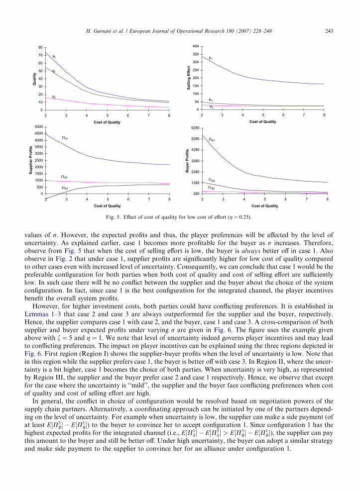
Fig. 5. Effect of cost of quality for low cost of effort (g = 0.25).


values of r. However, the expected profits and thus, the player preferences will be affected by the level ofuncertainty. As explained earlier, case 1 becomes more profitable for the buyer as r increases. Therefore,observe from Fig. 5 that when the cost of selling effort is low, the buyer is always better off in case 1. Alsoobserve in Fig. 2 that under case 1, supplier profits are significantly higher for low cost of quality comparedto other cases even with increased level of uncertainty. Consequently, we can conclude that case 1 would be thepreferable configuration for both parties when both cost of quality and cost of selling effort are sufficientlylow. In such case there will be no conflict between the supplier and the buyer about the choice of the systemconfiguration. In fact, since case 1 is the best configuration for the integrated channel, the player incentivesbenefit the overall system profits.

However, for higher investment costs, both parties could have conflicting preferences. It is established inLemmas 1–3 that case 2 and case 3 are always outperformed for the supplier and the buyer, respectively.Hence, the supplier compares case 1 with case 2, and the buyer, case 1 and case 3. A cross-comparison of bothsupplier and buyer expected profits under varying r are given in Fig. 6. The figure uses the example givenabove with f = 5 and g = 1. We note that level of uncertainty indeed governs player incentives and may leadto conflicting preferences. The impact on player incentives can be explained using the three regions depicted inFig. 6. First region (Region I) shows the supplier-buyer profits when the level of uncertainty is low. Note thatin this region while the supplier prefers case 1, the buyer is better off with case 3. In Region II, where the uncer-tainty is a bit higher, case 1 becomes the choice of both parties. When uncertainty is very high, as representedby Region III, the supplier and the buyer prefer case 2 and case 1 respectively. Hence, we observe that exceptfor the case where the uncertainty is ‘‘mild’’, the supplier and the buyer face conflicting preferences when costof quality and cost of selling effort are high.

In general, the conflict in choice of configuration would be resolved based on negotiation powers of thesupply chain partners. Alternatively, a coordinating approach can be initiated by one of the partners depend-ing on the level of uncertainty. For example when uncertainty is low, the supplier can make a side payment (ofat least E½P3

B� � E½P1B�) to the buyer to convince her to accept configuration 1. Since configuration 1 has the

highest expected profits for the integrated channel (i.e., E½P1S � � E½P3

S � > E½P3B� � E½P1

B�), the supplier can paythis amount to the buyer and still be better off. Under high uncertainty, the buyer can adopt a similar strategyand make side payment to the supplier to convince her for an alliance under configuration 1.

200

400

600

800

1000

1200

1400

1600

1800

2000

2200

0 10 20 30 40 50 60 70 80

Standard Deviation

Prof

its

S1

S2

B1

B3

Region II:Both supplier and buyer prefer case 1.

. . .

.

Region III: Supplier prefers case 2

Region I: Supplier

prefers case 1Buyer prefers

. Buyer prefers case 1

case 3

Π

Π

Π

Π

Fig. 6. Effect of uncertainty on supplier and buyer profits.


4.3. Centralized system solution

In the analysis so far, we considered the case where each firm maximized their individual profits only. Inthis section, we determine the optimal investment and pricing decisions for the integrated channel. The cen-tralized solution can be used as a reference in evaluating the potential benefits that a certain configurationcan bring to the channel partners. Clearly, in the centralized case there are only three decision variables: h,e, and p. The decisions are made in two stages. First, before the demand uncertainty is resolved, investmentdecisions h and e must be given. Second, the selling price, p is decided following the realization of the finaldemand potential. As usual, we start with the second stage objective function:

MaxðpÞ

PcðpÞ ¼ ðp � cð1þ vhÞÞða� p þ ceþ khþ nÞ � ge2

2� fh2

2

� �; ð44Þ

which at optimality yields

p�c ¼aþ ceþ khþ cð1þ vhÞ þ n

2: ð45Þ

Now, second stage expected channel profit is

E½Pcðh; eÞ� ¼ðaþ ceþ kh� cð1þ vhÞ þ nÞ2

4� ge2

2� fh2

2: ð46Þ

To ensure concavity, we need (f � K(k � cv)2) > 0, which also ensures that there are no pathological cases ofnegative quality or selling effort. Then, from first order optimality conditions we get:

h�c ¼Kða� cÞðk� cvÞf� Kðk� cvÞ2

; ð47Þ

e�c ¼fcKða� cÞ

gðf� Kðk� cvÞ2Þ: ð48Þ

Finally, the optimal expected channel profit is

E½P�c � ¼Kfða� cÞ2

2ðf� Kðk� cvÞ2Þþ r2

4: ð49Þ

750

1250

1750

2250

2750

3250

10 20 30 40 50 60 70 80

Standard Deviation

Inte

grat

ed C

hann

el P

rofit

s

c*

S1+ B1

S2+ B2

S3+ B3

Π

Π

Π

Π Π

Π

Π

Fig. 7. The gap between the integrated channel profits in the decentralized and centralized solutions as a function of r.


A comparison of (49) to case 1 profits reveals that the gap between the expected system optimal profit and theexpected integrated channel profit under case 1 stays constant in demand uncertainty. On the other hand, thegap between the expected integrated channel profits in the decentralized and the centralized solutions grows inr for both cases 2 and 3. This indicates that the value of configuration 1 and thus, its potential benefits to bothparties is higher under higher demand uncertainty. Fig. 7 illustrates the effect of demand uncertainty on thedifference in the integrated channel profits for the various configurations.

5. Conclusions

In supply chain co-opetition, firms both compete and co-operate with each other in order to maximize theirprofits. In this paper, we study the nature of co-operation between firms in making investments to improvedemand potential, as well as the competition between firms in making their pricing decisions. The incentivesof the co-opetition partners and the investment levels are mainly governed by the cost structure and the levelof uncertainty in the market. Our results can be summarized as follows:

• When the cost of quality and cost of selling effort are sufficiently low, both parties prefer configuration 1where the supplier commits to both the product quality investment and the wholesale price up-front.

• Under high cost of quality and cost of selling effort, the supplier still prefers configuration 1 if the uncer-tainty level is low. Otherwise, she is better off with configuration 2 where she postpones the wholesale pricedecision until after uncertainty is resolved. Under no circumstances would the supplier prefer configuration3 where she shares her first mover advantage with the buyer.

• Under high cost of selling effort the buyer may prefer configuration 3 if the uncertainty level is sufficientlylow. With high uncertainty, the buyer is better off with configuration 1 where he postpones his decisionsuntil the supplier makes all her commitments. Under no circumstances would the buyer prefer configura-tion 2.

• In all cases, integrated channel profits are the highest under configuration 1.• Configuration 2 will lead to the lowest product quality and effort commitments. Although, the highest sell-

ing efforts are employed in configuration 1, the comparison of quality in case 1 and case 3 depends on thecost of selling effort. The quality will be higher in configuration 1 if the cost of selling effort is sufficientlylow. Otherwise configuration 3 yields higher quality levels.

Our analysis indicates that if the supplier does not commit to the wholesale price before the market is devel-oped, the buyer will always under invest in his selling effort. This result is mainly due to the fear of supplieropportunism. Clearly, in such cases, the supplier can get a free ride on the buyer’s selling effort by charging ahigh wholesale price. It turns out that low investment in selling effort by the buyer eventually hurts the sup-plier’s profits, and the system as a whole. Consequently, we observe that the supplier prefers to be the leader


and make her pricing and quality investment decisions first when demand uncertainty is low. On the otherhand, if cost of selling effort is low, the buyer expects the supplier to free ride on his selling effort and henceprefers that the supplier commit to the wholesale price first. Based on this observation, we show that wheninvestment costs are sufficiently low, both parties prefer configuration 1. Thus, we conclude that with highinvestment costs, the level of demand uncertainty can lead to conflicting preferences for the supply chainpartners.

We note that the supply contract design problem in the paper is based on the notion of ‘‘co-opetition’’between the buyer and the supplier. As such, the supplier will not unilaterally choose a certain structure ifthe buyer is worse off under that structure.2 We discuss the issue of side-payments to reinforce the co-opetitivebehavior between the two firms. In the absence of co-opetition, the supplier would choose the contract thatgenerates the highest expected profit for him. Using the co-opetition approach, case 1 in the paper generatesthe highest expected profit for the supply chain as a whole and suitable distribution of profits can ensure thatboth firms prefer that arrangement.

The contribution of this paper is to study the effect of timing of price commitment decisions on the invest-ment decisions and on the profits for the two firms. While both the firms can benefit from each other’s invest-ment in product quality and selling effort, respectively, the timing of the price commitment decisions influencesthe level of investment by the firms. As such, the nature of competition between firms affects the level of co-operation they provide to each other. In future research, we plan to include the effect of information asym-metry in cost of quality and/or cost of selling effort in determining the optimal form of co-opetition betweenthe firms. Multi-period setting consideration is another interesting extension for future research

Appendix

Proof of Theorem 3.1. Since the objective functions of both players are continuous and concave, the existenceof equilibrium is established from the Theorem (Section 1.2) in Fudenberg and Tirole (1991). The uniquenessof equilibrium can be established through index theory approach. Index theory approach implies that if themultiplication of the slopes of the best response functions does not exceed one, then, if exists, the pure strategyequilibrium must be unique (see Cachon and Netessine, 1998 for details). Let P�B and P�S represent the profitfunctions given in (35) and (36) for the buyer and the supplier respectively. From implicit function theorem,slope of the best response function for the buyer, fB, is

2 ‘‘Ccontra

ofB

oh¼ o

2P�Boeoh

=o

2P�Boe2

¼ cðk� cvÞ8g� c2

and slope of the response function for the supplier, fS, is

ofS

oe¼ o2P�S

ohoe=o2P�Soh2

¼ cðk� cvÞ4f� ðk� cvÞ2

:

Consequently, the multiplication of the slopes is

ofB

ohofS

oe¼ c2ðk� cvÞ2

ð8g� c2Þð4f� ðk� cvÞ2Þ:

To prove that the equilibrium is unique, it is sufficient to show that the foregoing function is below one.Clearly, this is true if

ð8g� c2Þð4f� ðk� cvÞ2Þ > c2ðk� cvÞ2:

ontract pre-emption’’ by the supplier would be protested by the buyer as both parties are likely to first agree on the format of thect before determining the terms.


It is straightforward to see that the above inequality can be reduced to

f� K3ðk� cvÞ2 > 0:

Since this condition is assumed for concavity, the equilibrium is unique. h

Proof of Lemma 1. For part (a) of the lemma, note that h�1 > h�2, if

Kðk� cvÞða� cÞ2f� Kðk� cvÞ2

>K2

2ðk� cvÞða� cÞ2f� K2

2ðk� cvÞ2;

which, on simplification is true if K > 2K22. From the definitions of K and K2, we can show that K > 2K2

2, andhence, the quality offered by the supplier in case 1 is higher than the quality offered in case 2. Similarly, we canshow that e�1 > e�2.

For part (b), note that E½P�B1� > E½P�B2�, if

K2

fða� cÞð2f� Kðk� cvÞ2Þ

!2

>K2

8

fða� cÞðf� K2

2ðk� cvÞ2Þ

" #2

which, on simplification is true if K > 2K22. As noted above, K > 2K2

2, and hence, the buyer expects higherprofits in case 1 as compared to the profits in case 2. Similarly, E½P�S1� > E½P�S2�, if

fKða� cÞ2

2ð2f� Kðk� cvÞ2Þ>

fK22ða� cÞ2


þ r2

8:

Clearly, the inequality cannot hold for sufficiently high values of r implying that that case 1 is preferable to thesupplier when the uncertainty level is low enough. The expected integrated system profits are higher in case 1due to the fact that E½P�B1� þ E½P�S1� > E½P�B2� þ E½P�S2� from (11), (15), (21), and (23). h

Proof of Lemma 2. The proof of part (a) is due to the fact that 2K22 < K3 and follows from comparison of

(24)–(26), (27), (38)–(40), respectively. For part (b), note from (30) and (43) that E½P�B3� > E½P�B2� sinceK3 > K2

2. Also, E½P�S3� < E½P�S2�, if

ðfK22 � K2

3ðk� cvÞ2Þ fða� cÞ2

2ðf� K3ðk� cvÞ2Þ2<

fK22ða� cÞ2


:

The foregoing inequality can be reduced to ðK3 � K22Þ

2> 0, which clearly holds for K3and K2. Observe that the

last part of the lemma is true if E½P�B3� � E½P�B2� < E½P�S2� � E½P�S3�. This inequality can be reduced to

ð4K3 � 4K22 � K2Þðf� K2

2ðk� cvÞ2Þ > K2ðf� K3ðk� cvÞ2Þ;
which holds since K3 > K2
2. h

Proof of Lemma 3. For part (a) of the proof, note that h�1 > h�3 if

Kðk� cvÞða� cÞ2f� Kðk� cvÞ2

>K3ðk� cvÞða� cÞf� K3ðk� cvÞ2

;

which on simplification is true if K > 2K3. From the definitions of K and K3, we can show that K > 2K3 ifc2 < 2g < 3c2/2. and hence, the quality offered by the supplier in case 1 is higher than the quality offered incase 3, provided that the buyer’s cost of selling effort (g) is below a certain threshold. For higher values ofg, we have h�1 < h�3.

For part (b), the proof follows from comparing e�1 defined in (13) with e�3 defined in (38).For part (c) the first part of the proof directly follows from Lemmas 2 and 3. To prove the second part, we

first assume that n = 0. Second, we note that the supplier’s profits are decreasing in f in case 1 and increasing


in f in case 3, that is,oE½P1�

S �of < 0 and

oE½P�S3�of > 0. Since it is tedious to compare the general expressions for E½P�S1�

and E½P�S3�, we initially evaluate the limiting behavior as f!1.From (11), we have

E½P�S1jf!1� ¼Kða� cÞ2

4:

Similarly, from (42), we have

E½P�S3jf!1� ¼K2

2ða� cÞ2

2:

Then, E½P�S1jf!1� > E½P�S3jf!1� since K > 2K22. Further, since E½P�S1� is decreasing in f and E½P�S3� is increasing

in f, we have P�S1 > P�S3 for all f when n = 0. Observe from (11) and (42) that E½P�S1� � E½P�S3� decreases in rimplying that there exists a threshold value for r, above which expected profits in case 3 exceed case 1. Sincethe expected profits in the integrated channel are higher in case 1, the buyer profits must be lower when thesupplier profits are higher in case 3 compared to case 1. h

References

Anonymous, 2002. Cepheid names Isaza as European distributor of smart cycler. Worldwide Biotech 14 (7), 5–7.Amaldoss, W., Meyer, R.J., Raju, J.S., Rapoport, A., 2000. Collaborating to compete. Marketing Science 19 (2), 105–126.Anupindi, R., Bassok, Y., 1999. Supply contracts with quantity commitment and stochastic demand. In: Tayur, S., Ganeshan, R.,

Magazine, M. (Eds.), Quantitative Models for Supply Chain Management. Kluwer Academic Publishers., Norwell, MA, pp. 197–232.Banker, R.D., Khosla, I., Sinha, K.K., 1998. Quality and competition. Management Science 44 (9), 1179–1192.Brandenburger, A.M., Nalebuff, B.J., 1996. Co-opetition. Doubleday Currency, New York.Burton, T.M., 1998. Health care: Heart devices’ market battle is revving up. Wall Street Journal (September), B1.Cachon, G., Netessine, S., 1998. Game theory in supply chain analysis. In: Simchi-Levi, David, David Wu, S., Shen, Zuo-Jun (Max)

(Eds.), Handbook of Quantitative Supply Chain Analysis: Modeling in the eBusiness Era. Kluwer Academic Publishers.Canlen, B., 2002. Fluidmaster a straight flush in branding. Home Channel News 28 (15), 60–62.Desai, P.S., Srinivasan, K., 1995. A Franchise management issue: Demand signaling under unobservable service. Management Science 41

(10), 1608–1623.Desai, P.S., 1997. Advertising fee in business-format franchising. Management Science 43 (10), 1401–1419.Dyer, J.H., Singh, H., 1998. The relational view: Co-operative strategy and sources of inter-organizational competitive advantage.

Academy of Management Review 23, 660–679.Fudenberg, D., Tirole, J., 1991. Game Theory. MIT Press, Cambridge.Garvin, D.A., 1988. Managing Quality: The Strategic and Competitive Edge. The Free Press, New York.Gavirneni, S., Kapuscinski, R., Tayur, S., 1999. Value of Information of Capacitated Supply Chains. Management Science 45 (1), 16–24.Gnyawali, D.R., Madhavan, R., 2001. Co-operative Networks and Competitive Dynamics: A Structural Embeddedness Perspective.

Academy of Management Review 26, 431–445.Kern, T., 2002. Lowe’s takes aim: Lowe’s leans on vendors to build its brands. Home Channel News 28 (6), 38–40.Klein, B., Crawford, R., Alchian, A., 1978. Vertical integration, appropriable rents, and the competitive contracting process. The Journal

of Law and Economics 26, 297–326.Lado, A.A., Boyd, N.G., Hanlon, S.C., 1997. Competition, Co-operation, and the Search for Economic Rents: A Syncretic Model.

Academy of Management Review 22 (1), 110–141.Lal, R., 1990. Improving Channel Coordination Through Franchising. Marketing Science 9, 299–318.Luo, Y., 2004. Co-opetition in International Business. Copenhagen Business School Press, Copenhagen.Pasternack, B.A., 1985. Optimal Pricing and the Return Policy for Perishable Commodities. Marketing Science 4, 166–176.Savitski, D.W., 2002. Pricing in Competitive Electricity Markets. In: Faruqui, A., Eakin, K. (Eds.), Review of Industrial Organization.

21(3), pp. 329–333.

Documents

Impact of product pricing and timing of investment ... decisions as ﬁrms may not risk high investment in innovations due to the fear of opportunism by the other ﬁrm in setting