Documentos de Trabajo 65 - Facultad de Economía y Empresa …economiayempresa.udp.cl/wp-content/uploads/2016/08/WP65_Montero... · Documentos de Trabajo 65 How Important is Job Satisfaction

Documentos de Trabajo 65

How Important is Job Satisfaction in Life Satisfaction? Evidence from a Developing OECD Country

Álvaro MirandaUniversidad Diego Portales

Rodrigo MonteroUniversidad Diego Portales

Agosto 2015

How important is job satisfaction in life

satisfaction? Evidence from a developing OECD

country

Alvaro Miranda ∗ Rodrigo Montero†

July 5, 2015

Abstract

There is ample evidence about the determinants of life satisfaction and job satisfactionof individuals, however, there is less evidence about the importance of job satisfaction inlife satisfaction in economics. Using Chilean data, we estimate what are the effects ofdomain satisfactions in life satisfaction. Following the approach proposed by Van Praaget al. (2003), that takes into account the role of non-observables, we identify the relevantdomains for life satisfaction. Then, we construct a hierarchy to determine how importantis job satisfaction in life satisfaction. Results indicate that job satisfaction is the fourthdomain (of a total of 7 dimensions) in terms of importance for life satisfaction of chileanpeople. Also, we show that there is heterogeneity in this results by gender, age andeducational level. This suggest, that there are others domains that have to be study inorder to focus public policy that aims to enhance life satisfaction of individuals.

Keywords: Subjective well-being, job satisfaction, domain satisfactions.JEL Classification: C25, I31, J28.

∗[email protected]. Escuela de Ingenierıa Comercial, Universidad Diego Portales.†[email protected]. Departamento de Economıa, Universidad Diego Portales.

1 Introduction

In recent years, a great body of economic research has been developed in order to understand

the determinants of life satisfaction (Easterlin, 1973; Easterlin et al., 1974; Frijters et al., 2004;

Bjørnskov et al., 2008; Clark et al., 2008) and job satisfaction (Freeman, 1978; Clark, 1997;

Clark and Oswald, 1996; Hamermesh, 2001; Clark et al., 2009). Evidence suggests that life

satisfaction decrease with loosing a spouse, being recently fired, and it increases with income,

marriage and agency (Frijters et al., 2004; Hojman and Miranda, 2015). In particular, income

is not so important in absolute terms but in relative terms, i.e., individuals that have more

income than their reference group experience more wellbeing (Clark et al., 2008; Ferrer-i

Carbonell, 2005). In the case of job satisfaction, evidence suggest that labor conditions,

being male, the quantity of hours spend at work and wage are positively correlated with

it (Booth and Van Ours, 2008; Montero and Rau, 2015, ming). Moreover, the comparison

between individuals wage and their peer’s is important to explain it (Clark et al., 2009; Card

et al., 2012).

However, there has been little research in economics trying to understand the effect of job

satisfaction in life satisfaction. This relation seems important due to the fact that workers

spend a great proportion of their time in their jobs. Moreover, many studies in the psy-

chology field show an important link between job satisfaction and life satisfaction (Bowling

et al., 2010). Besides, it is also important to understand this link because it helps to focus

public policy in areas that allows to maximize welfare (Frey and Stutzer, 2002; Di Tella and

MacCulloch, 2006). This means that there could be others domains of life that could enhance

wellbeing more than being satisfied with job, implying that policy makers could focus their

investment in others domain rather than job.

The aim of this paper is to understand the importance of job satisfaction in life satisfaction

in Chile. The chilean case is interesting since it is a developing country which belongs to

the OECD. In terms of life satisfaction, Chileans have an average of 6.7 in the 0 to 10 scale,

which is very similar to the OECD average of 6.6. Nevertheless, labor characteristics are

remarkable different than the average of OECD countries. For instance, 62% of the working-

age population has a paid job, less than the 65% average of OECD countries. Also, people

work an average of 2,029 hours per year, which is very high in comparison with the average

2

of 1,765 hours worked in the OECD. Moreover, 15% of the workers work more than 50 hours

per week, which is 6 porcentual points greater than the average in the OECD. Finally, the

time spent in leisure and personal care, including sleeping and eating, is 14.41 hours per day,

which leads to being located in the 31 position over 36 countries of the OECD in this item.

To address this issue we use the chilean survey “Primera Encuesta Nacional de Condi-

ciones de Empleo, Trabajo, Salud y Calidad de Vida” (2009/10). This survey is representative

at national level of chilean workers. It contains information related with life satisfaction and

satisfaction with the following domains: privacy where you live, the amount of money you

earn, the amount of leisure, family life, indebtedness, health and job.

Our estimation procedure follows the “aggregating approach” (Ferrer-i Carbonell and

Van Praag, 2008) This approach arises in the context of a two-layer model. The first layer

provides that life satisfaction is the result of the satisfaction that is achieved in different

domains of life, such as work, health, family, etc. The second layer shows that each domain

in turn is determined by a set of exogenous variables.

The empirical implementation involves a two step procedure that allow us to build a

variable that accounts for non-observed heterogeneity (Van Praag et al., 2003). In the first

step we estimate the socioeconomic determinants of every domain of life by ordinary least

squares (OLS). Then, we predict the error terms of this estimations and we perform a principal

components analysis. Next, we extract the first principal component, which is the variable

that accounts for unobserved heterogeneity. In the second step we estimate an ordered probit

model of the relationship between life satisfaction, and job satisfaction, others satisfaction

domains and the first component of the principal components analysis.

Few studies have use the aggregating approach. Moreover, only a couple of them have

control by non-observed heterogeneity. For instance, Rojas (2006) follows the aggregating

approach, without controlling for unobserved heterogeneity, in order to get evidence for Mex-

ico. Their estimates show that economic satisfaction, health satisfaction, work satisfaction,

family satisfaction, and personal satisfaction are relevant to explain life satisfaction. Like-

wise, Easterlin and Sawangfa (2007) provide evidence for United States, not controlling for

unobserved heterogeneity. They found that financial satisfaction, health satisfaction, work

satisfaction, and family satisfaction are important for life satisfaction.

3

Closely related to our paper, Van Praag et al. (2003) use the GSOEP in order to identify

the main subjective domains for Germany. The authors found that job satisfaction, finan-

cial satisfaction, house satisfaction, health satisfaction, leisure satisfaction, and environment

satisfaction are important in terms of general satisfaction. Also, they find that results are sen-

sitive to the inclusion of the measure of non-observed heterogeneity. Also, Ferrer-i Carbonell

and Van Praag (2008) following the same approach as Van Praag et al. (2003) and using the

British Household Panel Survey (BHPS) found that job satisfaction, financial satisfaction,

housing satisfaction, health satisfaction, leisure-use satisfaction, leisure-amount satisfaction,

marriage satisfaction and social life satisfaction are relevant to explain life satisfaction.

Unlike previous studies, we want to understand which domain is more important to explain

life satisfaction. To do so, we standardize the estimated parameters, what allows us to build a

rank. Our estimates indicate that job satisfaction is the fourth domain of seven in importance

to explain life satisfaction. The most important domain is satisfaction with leisure, followed

by, family life and health. Our results suggest that investing in leisure, family life and health

could be more helpful in order to maximize welfare rather than job.

However, there is evidence that life satisfaction vary with demographic characteristics

(Easterlin, 2006; Rojas, 2007). Therefore, the importance of job satisfaction in life satisfaction

could vary with demographic characteristics of individuals. In order to explore this issue, we

procede to run separate estimates by gender, age and educational level. Our results indicate

that job satisfaction is the third domain in importance for man and the last domain for

woman. Also, job satisfaction is the fourth domain in importance for as both individuals

between 15-39 years old and individuals between 40-65 years old. Finally, job satisfaction is

the third domain of importance for individuals with primary and tertiary education. On the

other hand, job satisfaction is the fourth domain of importance for individuals with secondary

education. These results indicate, for instance, that public policy oriented to maximize job

satisfaction could be not very useful to maximize life satisfaction of woman.

Van Praag et al. (2003) concludes that “this study is a first step that has to be validated

on other data”. In line with this statement this paper contribute to the literature in mainly

three ways. First, we enhance the literature of subjective wellbeing for developing countries.

Second, we expand the existent literature by building a rank of domain satisfaction that

4

affects life satisfaction. This allows us to understand what can help to maximize welfare.

Finally, we explore the existence of heterogeneity in the relation of life satisfaction and job

satisfaction by gender, age and educational level.

The rest of the paper is organized as follows. Section 2 describes the data and methods.

Section 3 presents the results. Section 4 presents the discussion.

2 Data and Methods

2.1 Data

The main source for our data is the Primera Encuesta Nacional de Condiciones de Empleo,

Trabajo, Salud y Calidad de Vida 2009/10 (ENETS) . The ENETS is a cross section survey

that aims to describe and analyze the situation of the chilean workers population with respect

to employment conditions, work, health equity in order to help policy makers to design

better public policies in the field of employment, labour and social protection. The survey,

representative of workers at a national level, contains information from 9,502 workers on

different areas, such as education, household income, job characteristics, quality of life, etc.

Our sample will consist in white and blue collar workers between 15 and 65 years old.

In the quality of life section, the survey ask to rate on a scale of one to seven their life

satisfaction, the satisfaction with the privacy where they live, satisfaction with the amount

of money they earn, satisfaction with the amount of leisure, satisfaction with their family

life, satisfaction with their indebtedness, satisfaction with their health and job satisfaction.

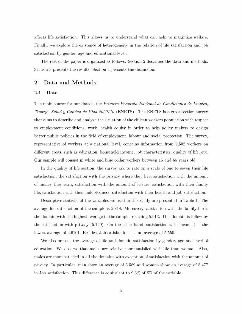
Descriptive statistic of the variables we used in this study are presented in Table 1. The

average life satisfaction of the sample is 5.818. Moreover, satisfaction with the family life is

the domain with the highest average in the sample, reaching 5.913. This domain is follow by

the satisfaction with privacy (5.749). On the other hand, satisfaction with income has the

lowest average of 4.6101. Besides, Job satisfaction has an average of 5.550.

We also present the average of life and domain satisfaction by gender, age and level of

education. We observe that males are relative more satisfied with life than woman. Also,

males are more satisfied in all the domains with exception of satisfaction with the amount of

privacy. In particular, man show an average of 5.589 and woman show an average of 5.477

in Job satisfaction. This difference is equivalent to 9.5% of SD of the variable.

5

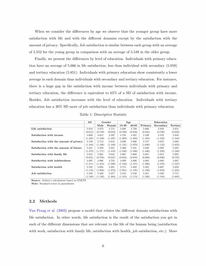
When we consider the differences by age we observe that the younger group have more

satisfaction with life and with the different domains except by the satisfaction with the

amount of privacy. Specifically, Job satisfaction is similar between each group with an average

of 5.552 for the young group in comparison with an average of 5.549 in the older group.

Finally, we present the differences by level of education. Individuals with primary educa-

tion have an average of 5.666 in life satisfaction, less than individual with secondary (5.859)

and tertiary education (5.851). Individuals with primary education show consistently a lower

average in each domain than individuals with secondary and tertiary education. For instance,

there is a huge gap in the satisfaction with income between individuals with primary and

tertiary education, the difference is equivalent to 65% of a SD of satisfaction with income.

Besides, Job satisfaction increases with the level of education. Individuals with tertiary

education has a 30% SD more of job satisfaction than individuals with primary education.

Table 1: Descriptive Statistic

All Gender Age Education

Male Female 15-39 40-65 Primary Secondary Tertiary

Life satisfaction 5.818 5.872 5.715 5.888 5.739 5.666 5.859 5.851(0.815) (0.749) (0.919) (0.769) (0.858) (0.845) (0.792) (0.823)

Satisfaction with income 4.609 4.615 4.597 4.735 4.467 4.100 4.570 5.043(1.445) (1.449) (1.437) (1.389) (1.492) (1.458) (1.422) (1.344)

Satisfaction with the amount of privacy 5.749 5.712 5.818 5.698 5.806 5.747 5.678 5.880(1.104) (1.100) (1.109) (1.131) (1.070) (1.030) (1.152) (1.053)

Satisfaction with the amount of leisure 5.241 5.359 5.021 5.366 5.101 5.038 5.298 5.285(1.273) (1.171) (1.419) (1.248) (1.286) (1.346) (1.250) (1.246)

Satisfaction with family life 5.913 5.961 5.825 5.961 5.860 5.801 5.913 5.995(0.831) (0.758) (0.947) (0.804) (0.858) (0.866) (0.836) (0.787)

Satisfaction with indebtedness 4.895 4.986 4.724 4.899 4.890 4.804 4.880 4.987(1.511) (1.454) (1.598) (1.546) (1.471) (1.566) (1.478) (1.527)

Satisfaction with health 5.558 5.694 5.301 5.714 5.382 5.325 5.607 5.633(1.119) (1.002) (1.273) (1.081) (1.135) (1.100) (1.053) (1.224)

Job satisfaction 5.550 5.589 5.477 5.552 5.549 5.351 5.539 5.715(1.180) (1.130) (1.264) (1.185) (1.174) (1.240) (1.194) (1.082)

Source: Author’s calculations based on ENETSNote: Standard errors in parentheses

2.2 Methods

Van Praag et al. (2003) propose a model that relates the different domain satisfactions with

life satisfaction. In other words, life satisfaction is the result of the satisfaction you get in

each of the different dimensions that are relevant to the life of the human being (satisfaction

with work, satisfaction with family life, satisfaction with health, job satisfaction, etc.). More

6

formally:

LS = f(DS1, DS2, ..., DSJ ;Z) (1)

where LS is life satisfaction, DS1, DS2, ..., DSJ represent the domains (work, health, fam-

ily life, etc.), and Z is an unobservable variable that affects general satisfaction. To complete

the model, the authors suggest that the domain satisfactions depend on individual’s objec-

tive situation (X) and on his or her personality (optimism) or other common unobservable

variable (Z); these personality traits are unobservables and they co-determine both LS and

DS. Therefore:

DSj = g(Xj ;Z) ∀j = 1, ..., J (2)

In this context if we estimate equation (1) and we do not control by Z we would have

endogeneity bias. Van Praag et al. (2003) propose to instrument Z through the following

procedure. After estimating the determinants of the J domains, they calculate the residuals

in order to estimate the part Z that is common to all the residuals. Then they get the

instrument as the first principal component of the J x J error covariance matrix. Then

adding this new variable as an additional covariate to the LS equation they can assume that

the remaining LS error is no longer correlated with the DS errors. Thus the estimators of

the coefficients in LS equation do not suffer from endogeneity bias.

Likewise, the first stage correspond to estimate by OLS the socioeconomic determinants

of the seven different domains satisfactions and we predict their residuals vectors. Then, we

perform a principal component analysis and we extract the first component, which is the

instrument for Z. The second stage consists in estimating an ordered probit model (1) using

the domains (DS1, DS2, ..., DSJ) and the instrument for Z as covariates.

Since the variables representing the domains are measures on a scale from one to seven,

then, 42 dummy variables should be included in the model. To avoid that, Ferrer-i Carbonell

and Van Praag (2008) propose to operationalize the DS variables (for both stages) by their

conditional expectations (assuming normality). Therefore, the following transformation is

applied:

7

DSj = E(DSj |µj,i−1 < DSj < µj,i) =n(µj,i−1)− n(µj,i)

N(µj,i)−N(µj,i−1)

where {(µj,i−1, µj,i)}Ii=1 are the intervals of the jth domain, and n(·) and N(·) represent

the pdf and cdf of a standard normal distribution.

Having estimated the model the question is to determine how important job satisfaction

is in life satisfaction. To do so, a hierarchy among the domain of satisfactions is constructed

in the following way. Remember that we have estimated an ordered probit model for life

satisfaction as follow:

LS∗ = α1DS1 + · · ·+ αJDSJ + βZ + ε

Hence, remember the marginal effects are given by:

∂E(LS∗|DS, Z)

∂DSj

= αj

It is direct to note that we can not establish which domain is more important simply

comparing the marginal effects. However, McKelvey and Zavoina (1975) propose to use

the standardized coefficients in order to interpreting the effect on dependent variable. The

standardized coefficients are constructed as follow:

α∗j = αj

(sjjsLS∗

)where sjj is the standard deviation of the regressor of interest, and sy∗ is the standard

deviation of y∗. With respect to the latter term note that with a model as follows:

LS∗ = γ′x+ ε

we have that:

var(LS∗) = γ′Σxxγ + σ2ε

Therefore, it is possible to determine a hierarchy that helps to understand how important

is job satisfaction in life satisfaction. Given the methodology has been presented now the

next section presents the main results.

8

3 Results

3.1 Socio-Demographic determinants of satisfaction domains

The first step of the methodology consist in estimate the socio-demographic determinants of

each satisfaction domain. We consider the following covariates as determinants of domain

satisfaction: dummy for woman, years of schooling, age (and squared), geographical dummies,

dummy for indigenous, log of income (or wage), number of people in household, dummy for

head of household, and dummies for marital status.

A key variable for the actual analysis are the incomes. Unfortunately, the data contains

only intervals of income. Each individual is ask to classify himself in one of the fourteen

predefined intervals. In the context of paper, this causes two difficulties. First, it forces

to incorporate thirteen dummy variables in the econometric model. Second, this makes it

impossible to build a reference wage to include it as a control in the domain of job satisfaction

which is very important according to empirical evidence in this area (Clark et al., 2009; Card

et al., 2012; Mumford and Smith, 2012; Montero and Vasquez, 2014; Montero and Rau, 2015).

In order to solve these problems, we propose to carry out an interval regression analysis

that will enable us to obtain a prediction for the individual wages and household incomes.

This strategy avoids the need to incorporate several dummy variables in the equations of the

domains, and allows us to take into account directly wage or income as covariates (for more

details see Montero and Vasquez (2014) )1.

We have done a special treatment for job satisfaction, since there is a lot of economic

research in this area that suggest a more complete model (Clark et al., 1996; Sousa-Poza

and Sousa-Poza, 2000; Assadullah and Fernandez, 2008; Booth and Van Ours, 2008; Clark

et al., 2009; Montero and Vasquez, 2014; Montero and Rau, 2015). Besides, our data is

very rich in terms of labor information. Hence we have included the following covariates

for DS5: dummy for woman, years of schooling, age (and squared), geographical dummies,

dummy for indigenous, dummy for first job, dummy for unionized, wage (in logs), travel

1A key aspect is the choice of variables that are determinants of wages (or income) within the interval.As Montero and Vasquez (2014) we use years of schooling, age (and squared) and a dummy for woman ascovariates for wages. On the other hand, for estimating the household income we use information of thehousehold head (years of schooling, age, squared age, dummy for woman) and household (number of peoplein household, number of people who contribute to the household income, and geographical dummies) ascovariates.

9

time to work, dummy for having a contract, dummy for invoice, hours worked (also in logs),

dummy for working in public sector, dummy for contributing to retirement pension, dummy

for contributing to social health system, promotion opportunities, workplace, environmental

conditions of work, dummy for individual outsourced, dummy for fixed wage, dummy if

individual works from home, and a variable that measures the wage of reference group. For

this last variable we follow the methodology proposed by Ferrer-i Carbonell (2005) which

consists of constructing the reference group using information of two key variables. We used

information related to economic activity (grouped in nine activities) and schooling.

This last variable we splitted in five categories: no schooling or incomplete basic education,

complete basic education, incomplete high school, complete high school, and college. When

we combine the information from these two variables (economic activity and schooling) we

get 45 cells and then we proceed to calculate the average wage for every single cell. That

average wage correspond to the reference wage for the individual belonging to that specific

cell. The sign for the coefficient of this variable could be positive or negative depending on

which effect dominates, the comparison effect or the information effect2.

Table 2 presents the estimations of the sociodemographic determinants of each satisfac-

tion domain. The first column of Table 2 show that income satisfaction increase with the

logarithm of income. Also, married, widower and single individuals are more satisfied with

income than separated. Finally, woman are less satisfied with income than man. The second

column show the sociodemographic determinants of satisfaction with the amount of privacy.

Results indicate that the logarithm of income and the years of schooling increase this domain

satisfaction. On the contrary, the more number of people in the household, less satisfaction.

The third column of Table 2 present the determinants of the satisfaction with the amount

of leisure. Results show that woman are less satisfied with the amount of leisure than man.

Satisfaction with this domain increases with the logarithm of income and years of schooling,

but decrease with age and the number of individuals that live at home.Finally, married and

2It seems reasonable to think that actually there is a negative relationship between relative wage andindividual job satisfaction; that has been called the comparison effect (Clark et al., 2009; Card et al., 2012;Mumford and Smith, 2012). However, more recently the literature has revealed a different potential relation-ship between relative wage and job satisfaction. In effect, Clark et al. (2009) argue that a higher referencegroup wage level (something like the wage of my peers) could increase job satisfaction because it reveals valu-able information about the future prospects. The higher the future wage prospects, the higher the level of jobsatisfaction. This phenomenon has been called the information effect (Manski, 2000).

10

single people are more satisfied with the amount of fun than separated.

11

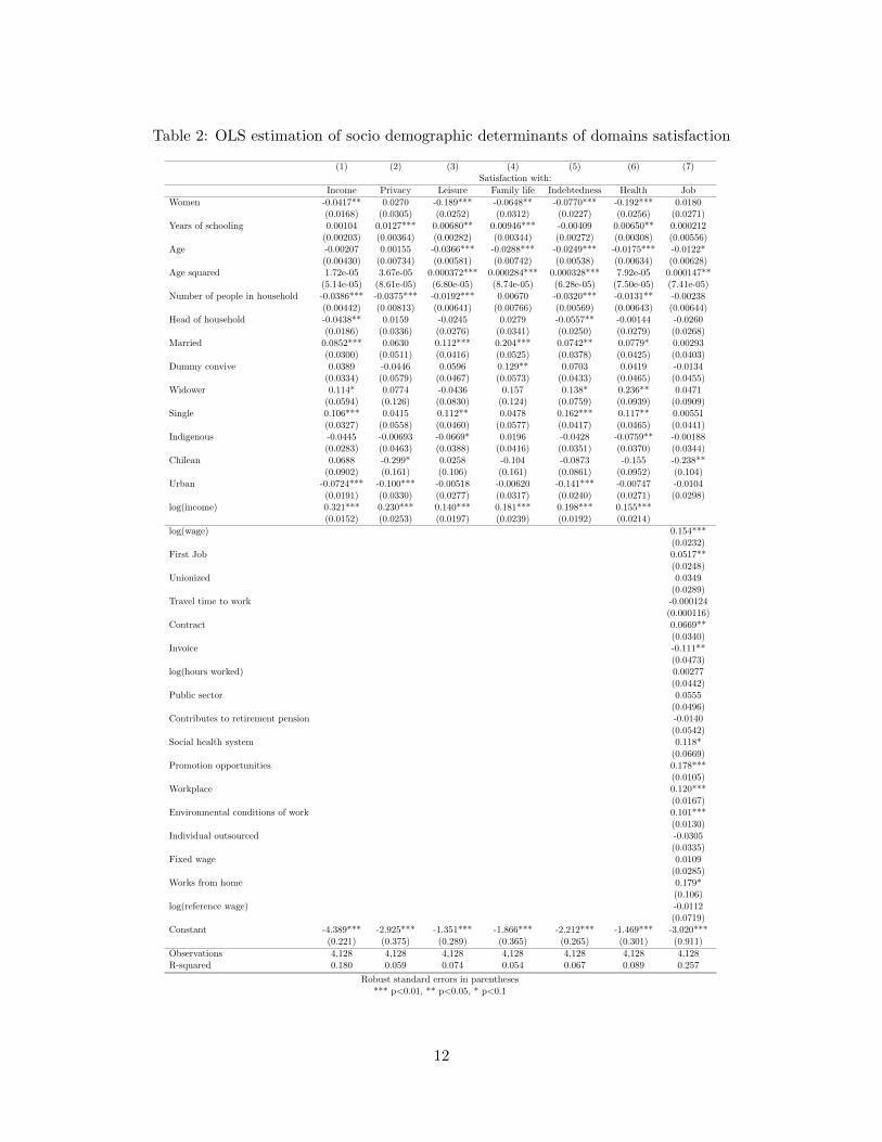
Table 2: OLS estimation of socio demographic determinants of domains satisfaction

(1) (2) (3) (4) (5) (6) (7)Satisfaction with:

Income Privacy Leisure Family life Indebtedness Health Job

Women -0.0417** 0.0270 -0.189*** -0.0648** -0.0770*** -0.192*** 0.0180(0.0168) (0.0305) (0.0252) (0.0312) (0.0227) (0.0256) (0.0271)

Years of schooling 0.00104 0.0127*** 0.00680** 0.00946*** -0.00409 0.00650** 0.000212(0.00203) (0.00364) (0.00282) (0.00344) (0.00272) (0.00308) (0.00556)

Age -0.00207 0.00155 -0.0366*** -0.0288*** -0.0249*** -0.0175*** -0.0122*(0.00430) (0.00734) (0.00581) (0.00742) (0.00538) (0.00634) (0.00628)

Age squared 1.72e-05 3.67e-05 0.000372*** 0.000284*** 0.000328*** 7.92e-05 0.000147**(5.14e-05) (8.61e-05) (6.80e-05) (8.74e-05) (6.28e-05) (7.50e-05) (7.41e-05)

Number of people in household -0.0386*** -0.0375*** -0.0192*** 0.00670 -0.0320*** -0.0131** -0.00238(0.00442) (0.00813) (0.00641) (0.00766) (0.00569) (0.00643) (0.00644)

Head of household -0.0438** 0.0159 -0.0245 0.0279 -0.0557** -0.00144 -0.0260(0.0186) (0.0336) (0.0276) (0.0341) (0.0250) (0.0279) (0.0268)

Married 0.0852*** 0.0630 0.112*** 0.204*** 0.0742** 0.0779* 0.00293(0.0300) (0.0511) (0.0416) (0.0525) (0.0378) (0.0425) (0.0403)

Dummy convive 0.0389 -0.0446 0.0596 0.129** 0.0703 0.0419 -0.0134(0.0334) (0.0579) (0.0467) (0.0573) (0.0433) (0.0465) (0.0455)

Widower 0.114* 0.0774 -0.0436 0.157 0.138* 0.236** 0.0471(0.0594) (0.126) (0.0830) (0.124) (0.0759) (0.0939) (0.0909)

Single 0.106*** 0.0415 0.112** 0.0478 0.162*** 0.117** 0.00551(0.0327) (0.0558) (0.0460) (0.0577) (0.0417) (0.0465) (0.0441)

Indigenous -0.0445 -0.00693 -0.0669* 0.0196 -0.0428 -0.0759** -0.00188(0.0283) (0.0463) (0.0388) (0.0416) (0.0351) (0.0370) (0.0344)

Chilean 0.0688 -0.299* 0.0258 -0.104 -0.0873 -0.155 -0.238**(0.0902) (0.161) (0.106) (0.161) (0.0861) (0.0952) (0.104)

Urban -0.0724*** -0.100*** -0.00518 -0.00620 -0.141*** -0.00747 -0.0104(0.0191) (0.0330) (0.0277) (0.0317) (0.0240) (0.0271) (0.0298)

log(income) 0.321*** 0.230*** 0.140*** 0.181*** 0.198*** 0.155***(0.0152) (0.0253) (0.0197) (0.0239) (0.0192) (0.0214)

log(wage) 0.154***(0.0232)

First Job 0.0517**(0.0248)

Unionized 0.0349(0.0289)

Travel time to work -0.000124(0.000116)

Contract 0.0669**(0.0340)

Invoice -0.111**(0.0473)

log(hours worked) 0.00277(0.0442)

Public sector 0.0555(0.0496)

Contributes to retirement pension -0.0140(0.0542)

Social health system 0.118*(0.0669)

Promotion opportunities 0.178***(0.0105)

Workplace 0.120***(0.0167)

Environmental conditions of work 0.101***(0.0130)

Individual outsourced -0.0305(0.0335)

Fixed wage 0.0109(0.0285)

Works from home 0.179*(0.106)

log(reference wage) -0.0112(0.0719)

Constant -4.389*** -2.925*** -1.351*** -1.866*** -2.212*** -1.469*** -3.020***(0.221) (0.375) (0.289) (0.365) (0.265) (0.301) (0.911)

Observations 4,128 4,128 4,128 4,128 4,128 4,128 4,128R-squared 0.180 0.059 0.074 0.054 0.067 0.089 0.257

Robust standard errors in parentheses*** p<0.01, ** p<0.05, * p<0.1

12

The determinants of satisfaction with family life are presented in the fourth column of

Table 2. Satisfaction with family life increases with the logarithm of income and years of

schooling. However, it decreases with age. Also, Married and cohabitants are more satisfied

than separated people with their family life.

The fifth column of Table 2 presentes the determinants of job satisfaction. The more

wage individuals earn more satisfied are. Also, individuals with contract are more satisfied

than individuals without a formal work. On the other hand individuals that work with

invoice are less satisfied than individuals without a formal work. Besides, the characteristic

of work are relevant in order to enjoy more satisfaction. Having promotion opportunities, a

good workplace and better environmental conditions at work are correlated with more job

satisfaction.

Column (6) of Table 2 present the determinants of the satisfaction with the level of indebt-

edness. Results indicate that this domain satisfaction increases with income and decreases

with the number of individuals that live at home and age. Also, Woman ares less satisfied

with indebtedness than man. Finally, married and single individuals are more satisfied than

separated individuals. Finally, column (7) of Table 2 presents the determinants of health

satisfaction. Individuals with more years of schooling and more income are more satisfied

with their health. Also, Woman are less satisfied with their health than man.

It is important to highlight that the goodness of fit of the regressions for each of the

domains is in the expected range. For instance, Van Praag et al. (2003) report R squared

going between 2 and 20 percent. In our cases, the R squared goes from 5 to 26 percent. This

helps to assure that the information contain in the error term are non observe variables.

After estimating the determinants of each domain satisfaction, we predict the residuals of

each regression. The correlation between the residuals of each regression is shown in Table 3.

The correlation between each residuals vary between 17.5% to 41.5%, suggesting that there

are common non observe variables in the residuals.

13

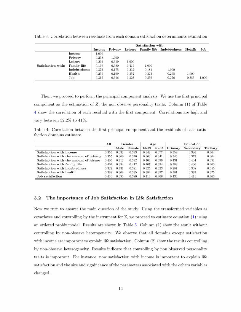
Table 3: Correlation between residuals from each domain satisfaction determinants estimation

Satisfaction with:Income Privacy Leisure Family life Indebtedness Heatlh Job

Satisfaction with:

Income 1,000Privacy 0,258 1,000Leisure 0,291 0,319 1,000Family life 0,197 0,380 0,415 1,000Indebtedness 0,373 0,175 0,232 0,181 1,000Health 0,255 0,199 0,352 0,373 0,265 1,000Job 0,315 0,316 0,323 0,356 0,276 0,385 1,000

Then, we proceed to perform the principal component analysis. We use the first principal

component as the estimation of Z, the non observe personality traits. Column (1) of Table

4 show the correlation of each residual with the first component. Correlations are high and

vary between 32.2% to 41%.

Table 4: Correlation between the first principal component and the residuals of each satis-faction domains estimate



Satisfaction with income 0.355 0.332 0.393 0.342 0.377 0.359 0.326 0.404Satisfaction with the amount of privacy 0.355 0.360 0.346 0.363 0.341 0.346 0.379 0.304Satisfaction with the amount of leisure 0.405 0.412 0.392 0.406 0.399 0.431 0.404 0.391Satisfaction with family life 0.402 0.394 0.412 0.407 0.394 0.388 0.406 0.403Satisfaction with indebtedness 0.322 0.431 0.381 0.325 0.323 0.287 0.308 0.355Satisfaction with health 0.388 0.308 0.335 0.382 0.397 0.381 0.399 0.375Job satisfaction 0.410 0.393 0.380 0.410 0.406 0.433 0.411 0.403

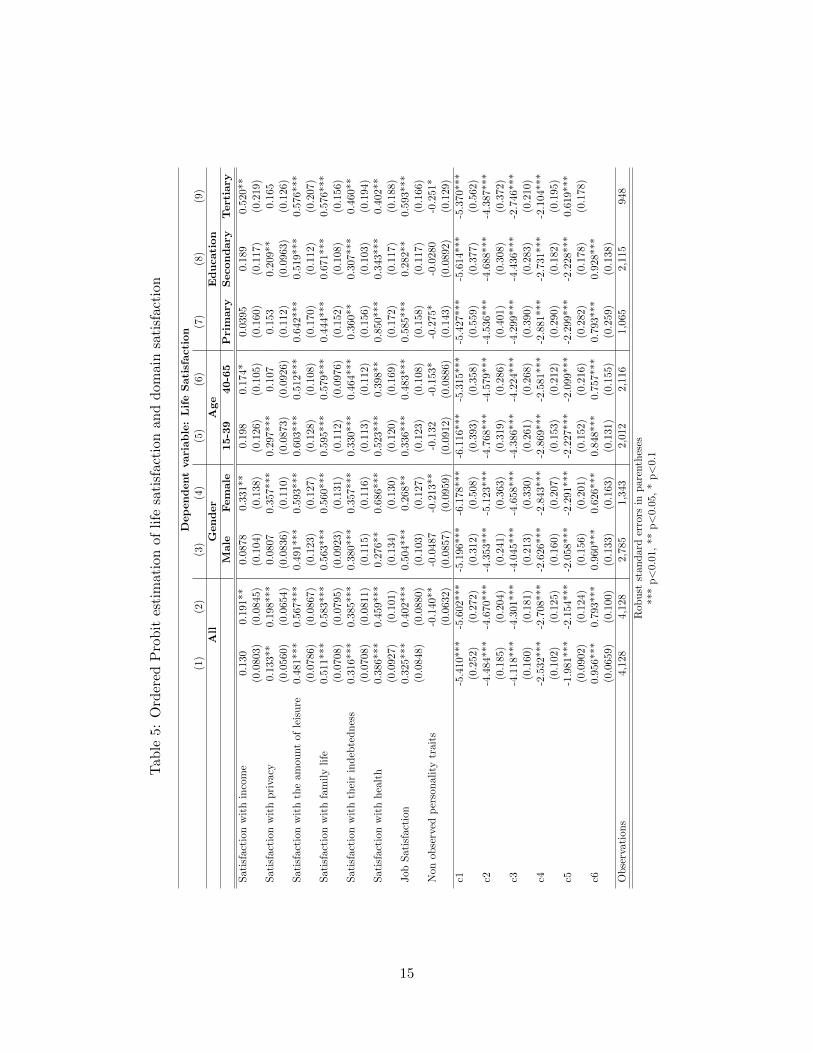
3.2 The importance of Job Satisfaction in Life Satisfaction

Now we turn to answer the main question of the study. Using the transformed variables as

covariates and controlling by the instrument for Z, we proceed to estimate equation (1) using

an ordered probit model. Results are shown in Table 5. Column (1) show the result without

controlling by non-observe heterogeneity. We observe that all domains except satisfaction

with income are important to explain life satisfaction. Column (2) show the results controlling

by non-observe heterogeneity. Results indicate that controlling by non observed personality

traits is important. For instance, now satisfaction with income is important to explain life

satisfaction and the size and significance of the parameters associated with the others variables

changed.

14

Tab

le5:

Ord

ered

Pro

bit

esti

mat

ion

oflife

sati

sfac

tion

and

dom

ain

sati

sfac

tion

Dep

en

dent

vari

able

:L

ife

Sati

sfacti

on

(1)

(2)

(3)

(4)

(5)

(6)

(7)

(8)

(9)

All

Gen

der

Age

Ed

ucati

on

Male

Fem

ale

15-3

940-6

5P

rim

ary

Secon

dary

Tert

iary

Sat

isfa

ctio

nw

ith

inco

me

0.13

00.

191*

*0.

0878

0.33

1**

0.1

980.

174*

0.0

395

0.1

890.5

20**

(0.0

803)

(0.0

845)

(0.1

04)

(0.1

38)

(0.1

26)

(0.1

05)

(0.1

60)

(0.1

17)

(0.2

19)

Sat

isfa

ctio

nw

ith

pri

vacy

0.13

3**

0.19

8***

0.08

070.3

57***

0.29

7**

*0.

107

0.1

53

0.209

**0.1

65

(0.0

560)

(0.0

654)

(0.0

836)

(0.1

10)

(0.0

873

)(0

.092

6)(0

.112)

(0.0

963

)(0

.126)

Sat

isfa

ctio

nw

ith

the

amou

nt

ofle

isure

0.48

1***

0.56

7***

0.49

1***

0.59

3***

0.60

3**

*0.5

12***

0.6

42***

0.519

***

0.5

76***

(0.0

786)

(0.0

867)

(0.1

23)

(0.1

27)

(0.1

28)

(0.1

08)

(0.1

70)

(0.1

12)

(0.2

07)

Sat

isfa

ctio

nw

ith

fam

ily

life

0.51

1***

0.58

3***

0.56

3***

0.56

0***

0.59

5**

*0.5

79***

0.4

44***

0.671

***

0.5

76***

(0.0

708)

(0.0

795)

(0.0

923)

(0.1

31)

(0.1

12)

(0.0

976)

(0.1

52)

(0.1

08)

(0.1

56)

Sat

isfa

ctio

nw

ith

thei

rin

deb

tednes

s0.

316*

**0.

385*

**0.

380*

**0.

357*

**

0.33

0**

*0.4

64***

0.36

0**

0.3

07*

**

0.4

60**

(0.0

708)

(0.0

811)

(0.1

15)

(0.1

16)

(0.1

13)

(0.1

12)

(0.1

56)

(0.1

03)

(0.1

94)

Sat

isfa

ctio

nw

ith

hea

lth

0.38

6***

0.45

9***

0.27

6**

0.686

***

0.52

3**

*0.

398**

0.8

50***

0.343

***

0.4

02**

(0.0

927)

(0.1

01)

(0.1

34)

(0.1

30)

(0.1

20)

(0.1

69)

(0.1

72)

(0.1

17)

(0.1

88)

Job

Sat

isfa

ctio

n0.

325*

**0.

402*

**0.

504*

**0.

268

**0.

336**

*0.4

83***

0.5

85***

0.2

82*

*0.5

93***

(0.0

848)

(0.0

880)

(0.1

03)

(0.1

27)

(0.1

23)

(0.1

08)

(0.1

58)

(0.1

17)

(0.1

66)

Non

obse

rved

per

sonal

ity

trai

ts-0

.140

**-0

.048

7-0

.213

**

-0.1

32-0

.153*

-0.2

75*

-0.0

280

-0.2

51*

(0.0

632)

(0.0

857)

(0.0

959)

(0.0

912

)(0

.088

6)(0

.143)

(0.0

892

)(0

.129)

c1-5

.410

***

-5.6

02**

*-5

.196

***

-6.1

78***

-6.1

16**

*-5

.315

***

-5.4

27**

*-5

.614

***

-5.3

70***

(0.2

52)

(0.2

72)

(0.3

12)

(0.5

08)

(0.3

93)

(0.3

58)

(0.5

59)

(0.3

77)

(0.5

62)

c2-4

.484

***

-4.6

70**

*-4

.353

***

-5.1

23***

-4.7

68**

*-4

.579

***

-4.5

36**

*-4

.688

***

-4.3

87***

(0.1

85)

(0.2

04)

(0.2

41)

(0.3

63)

(0.3

19)

(0.2

86)

(0.4

01)

(0.3

08)

(0.3

72)

c3-4

.118

***

-4.3

01**

*-4

.045

***

-4.6

58***

-4.3

86**

*-4

.224

***

-4.2

99**

*-4

.436

***

-2.7

46***

(0.1

60)

(0.1

81)

(0.2

13)

(0.3

30)

(0.2

61)

(0.2

68)

(0.3

90)

(0.2

83)

(0.2

10)

c4-2

.532

***

-2.7

08**

*-2

.626

***

-2.8

43***

-2.8

69**

*-2

.581

***

-2.8

81**

*-2

.731

***

-2.1

04***

(0.1

02)

(0.1

25)

(0.1

60)

(0.2

07)

(0.1

53)

(0.2

12)

(0.2

90)

(0.1

82)

(0.1

95)

c5-1

.981

***

-2.1

54**

*-2

.058

***

-2.2

91***

-2.2

27**

*-2

.099

***

-2.2

99**

*-2

.228

***

0.619***

(0.0

902)

(0.1

24)

(0.1

56)

(0.2

01)

(0.1

52)

(0.2

16)

(0.2

82)

(0.1

78)

(0.1

78)

c60.

956*

**0.

793*

**0.

960*

**0.

626*

**

0.84

8**

*0.7

57***

0.7

93***

0.928

***

(0.0

659)

(0.1

00)

(0.1

33)

(0.1

63)

(0.1

31)

(0.1

55)

(0.2

59)

(0.1

38)

Obse

rvat

ions

4,12

84,

128

2,78

51,3

432,0

122,

116

1,0

65

2,115

948

Rob

ust

stan

dar

der

rors

inpare

nth

eses

***

p<

0.01

,**

p<

0.05

,*

p<

0.1

15

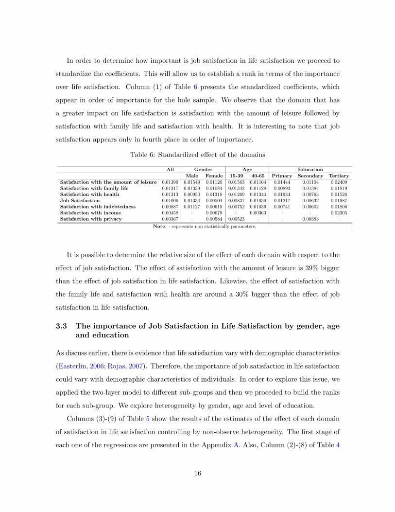
In order to determine how important is job satisfaction in life satisfaction we proceed to

standardize the coefficients. This will allow us to establish a rank in terms of the importance

over life satisfaction. Column (1) of Table 6 presents the standardized coefficients, which

appear in order of importance for the hole sample. We observe that the domain that has

a greater impact on life satisfaction is satisfaction with the amount of leisure followed by

satisfaction with family life and satisfaction with health. It is interesting to note that job

satisfaction appears only in fourth place in order of importance.

Table 6: Standardized effect of the domains



Satisfaction with the amount of leisure 0.01399 0.01549 0.01120 0.01563 0.01104 0.01444 0.01104 0.02409Satisfaction with family life 0.01317 0.01339 0.01084 0.01343 0.01128 0.00893 0.01384 0.01819Satisfaction with health 0.01313 0.00950 0.01318 0.01269 0.01344 0.01934 0.00763 0.01526Job Satisfaction 0.01006 0.01334 0.00504 0.00837 0.01039 0.01217 0.00632 0.01987Satisfaction with indebtedness 0.00887 0.01127 0.00615 0.00752 0.01036 0.00741 0.00602 0.01806Satisfaction with income 0.00458 · 0.00679 · 0.00363 · · 0.02305Satisfaction with privacy 0.00367 · 0.00584 0.00523 · · 0.00383 ·

Note: · represents non statistically parameters.

It is possible to determine the relative size of the effect of each domain with respect to the

effect of job satisfaction. The effect of satisfaction with the amount of leisure is 39% bigger

than the effect of job satisfaction in life satisfaction. Likewise, the effect of satisfaction with

the family life and satisfaction with health are around a 30% bigger than the effect of job

satisfaction in life satisfaction.

3.3 The importance of Job Satisfaction in Life Satisfaction by gender, ageand education

As discuss earlier, there is evidence that life satisfaction vary with demographic characteristics

(Easterlin, 2006; Rojas, 2007). Therefore, the importance of job satisfaction in life satisfaction

could vary with demographic characteristics of individuals. In order to explore this issue, we

applied the two-layer model to different sub-groups and then we proceded to build the ranks

for each sub-group. We explore heterogeneity by gender, age and level of education.

Columns (3)-(9) of Table 5 show the results of the estimates of the effect of each domain

of satisfaction in life satisfaction controlling by non-observe heterogeneity. The first stage of

each one of the regressions are presented in the Appendix A. Also, Column (2)-(8) of Table 4

16

show the correlation of each residual with the first principal component use as the estimation

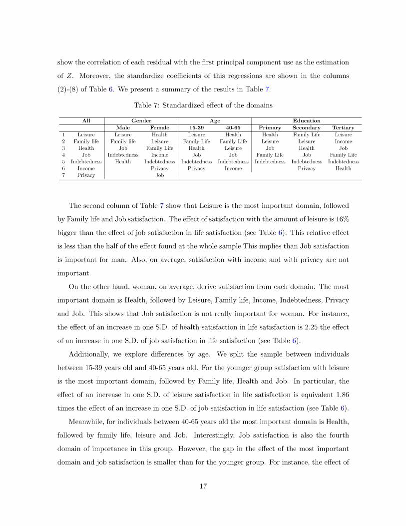
of Z. Moreover, the standardize coefficients of this regressions are shown in the columns

(2)-(8) of Table 6. We present a summary of the results in Table 7.

Table 7: Standardized effect of the domains



1 Leisure Leisure Health Leisure Health Health Family Life Leisure2 Family life Family life Leisure Family Life Family Life Leisure Leisure Income3 Health Job Family Life Health Leisure Job Health Job4 Job Indebtedness Income Job Job Family Life Job Family Life5 Indebtedness Health Indebtedness Indebtedness Indebtedness Indebtedness Indebtedness Indebtedness6 Income Privacy Privacy Income Privacy Health7 Privacy Job

The second column of Table 7 show that Leisure is the most important domain, followed

by Family life and Job satisfaction. The effect of satisfaction with the amount of leisure is 16%

bigger than the effect of job satisfaction in life satisfaction (see Table 6). This relative effect

is less than the half of the effect found at the whole sample.This implies than Job satisfaction

is important for man. Also, on average, satisfaction with income and with privacy are not

important.

On the other hand, woman, on average, derive satisfaction from each domain. The most

important domain is Health, followed by Leisure, Family life, Income, Indebtedness, Privacy

and Job. This shows that Job satisfaction is not really important for woman. For instance,

the effect of an increase in one S.D. of health satisfaction in life satisfaction is 2.25 the effect

of an increase in one S.D. of job satisfaction in life satisfaction (see Table 6).

Additionally, we explore differences by age. We split the sample between individuals

between 15-39 years old and 40-65 years old. For the younger group satisfaction with leisure

is the most important domain, followed by Family life, Health and Job. In particular, the

effect of an increase in one S.D. of leisure satisfaction in life satisfaction is equivalent 1.86

times the effect of an increase in one S.D. of job satisfaction in life satisfaction (see Table 6).

Meanwhile, for individuals between 40-65 years old the most important domain is Health,

followed by family life, leisure and Job. Interestingly, Job satisfaction is also the fourth

domain of importance in this group. However, the gap in the effect of the most important

domain and job satisfaction is smaller than for the younger group. For instance, the effect of

17

an increase in one S.D. of health satisfaction in life satisfaction is equivalent 1.29 times the

effect of an increase in one S.D. of job satisfaction in life satisfaction (see Table 6).

Finally, we explore the differences by educational level. For individuals with primary

education health is the most important domain, followed by leisure and job. On the other

hand, for individuals with secondary education Family life is the most important domain,

followed by leisure, health and Job. Finally, for individuals with tertiary education leisure is

the most important domain, followed by income an job. Is interesting to note that satisfaction

with income is only relevant for individuals with tertiary education. Moreover, in this group

is the second domain of importance.

In the case of individuals with primary education the effect of an increase in one S.D.

in satisfaction with leisure in life satisfaction is equivalent to 1.59 times the effect of an

increase in one S.D. of Job satisfaction in life satisfaction. On the other hand, the effect of

an increase in one S.D. in satisfaction with family life in life satisfaction for individuals with

secondary education is 2.19 times the effect of and increase in one S.D. of Job satisfaction

in life satisfaction. Finally, for individuals with tertiary education the effect of an increase

in one S.D. in satisfaction with leisure is equivalent to 1.21 times the effect of an increase in

one S.D. of Job satisfaction in life satisfaction.

4 Discussion

In this paper we investigate the importance of job satisfaction in life satisfaction of a sample

of chileans white and blue collar workers between 15 and 65 years old. Using the aggregating

approach (Van Praag et al., 2003) and controlling by non observe heterogeneity, we find that

job satisfaction is the fourth domain in importance to explain life satisfaction of a total of

seven. The most important domain is satisfaction with leisure, followed by satisfaction with

family life and satisfaction with health.

Moreover, we investigate how this relation varies by gender, age and educational level.

Results indicate that for males, job satisfaction is the third domain in importance to explain

life satisfaction. On the other hand, for woman, job satisfaction is the seventh domain of

importance. In the case of age, job satisfaction is the fourth domain of importance in both

sub-samples, i.e, individuals between 15-39 years old and individuals between 40-65 years old.

18

Finally, job satisfaction is in the third place of importance for individuals with primary and

tertiary education. However, for individuals with secondary education job satisfaction is the

fourth domain in importance.

Our results suggest, first, that there are other domains more important than job satisfac-

tion where public policy could be oriented in order to enhance the wellbeing of individuals

(Frey and Stutzer, 2002; Di Tella and MacCulloch, 2006). Second, there is heterogeneity in

the importance of job satisfaction in life satisfaction across groups in the population. For

instance, job satisfaction in the least important domain for woman. This suggest that in

order to promote welfare in the population, policy makers must take into account the charac-

teristics of individuals. Third, in light with the fact that individuals work relatively a lot of

hours in Chile and they have little time for leisure, this results indicate that there is a need

in order to increase the time and resources to expend in order activities different than job.

Finally, there is an important open research agenda in order to understand what determines

each of the satisfaction domain, different than job satisfaction, with more accuracy, with the

objective to identified the variables that could be changed through public policy to enhance

those satisfaction domains and, therefore, enhance life satisfaction.

19

References

Assadullah, M. and Fernandez, R. (2008). Work-life balance practices and the gender gap in

job satisfaction in the uk: Evidence from matched employer-employee data. IZA discussion

paper series, (3582).

Bjørnskov, C., Dreher, A., and Fischer, J. A. (2008). Cross-country determinants of life

satisfaction: Exploring different determinants across groups in society. Social Choice and

Welfare, 30(1):119–173.

Booth, A. and Van Ours, J. (2008). Job satisfaction and family happiness: the part-time

work puzzle. The Economic Journal, 118:77–99.

Bowling, N. A., Eschleman, K. J., and Wang, Q. (2010). A meta-analytic examination of the

relationship between job satisfaction and subjective well-being. Journal of Occupational

and Organizational Psychology, 83(4):915–934.

Card, D., Mas, A., Moretti, E., and Saez, E. (2012). Inequality at work: the effect of peer

salaries on job satisfaction. Amerincan Economic Review, 102(6).

Clark, A. (1997). Job satisfaction and gender. why are women so happy at work? Labour

Economics, 4(4):341–372.

Clark, A., Frijters, P., and Shields, M. (2008). Relative income, happiness and utility: an

explanation for the easterlin paradox and other puzzles. Journal of Economic Literature,

46(1):95–144.

Clark, A. and Oswald, A. (1996). Satisfaction and comparison income. Journal of Public

Economics, 61:359–381.

Clark, A., Oswald, A., and Warr, P. (1996). Is job satisfaction u-shaped in age? Journal of

Occupational and Organizational Psychology, 69:57–81.

Clark, A. E., Kristensen, N., and Westergard-Nielsen, N. (2009). Job satisfaction and co-

worker wages: Status or signal?*. The Economic Journal, 119(536):430–447.

20

Di Tella, R. and MacCulloch, R. (2006). Some uses of happiness data in economics. The

Journal of Economic Perspectives, pages 25–46.

Easterlin, R. (1973). Does money buy happiness? The Public Interest, 30:3–10.

Easterlin, R., David, P., and Reder, M. (1974). Does economic growth improve the human

lot? Some empirical evidence. New York Academic Press.

Easterlin, R. A. (2006). Life cycle happiness and its sources: Intersections of psychology,

economics, and demography. Journal of Economic Psychology, 27(4):463–482.

Easterlin, R. A. and Sawangfa, O. (2007). Happiness and domain satisfaction: Theory and

evidence. IZA Discussion Papers 2584, Institute for the Study of Labor (IZA).

Ferrer-i Carbonell, A. (2005). Income and well-being: An empirical analysis of the comparison

income effect. Journal of Public Economics, 89:997–1019.

Ferrer-i Carbonell, A. and Van Praag, B. (2008). Happiness Quantified. A satisfaction calculus

approach. Oxford University Press.

Freeman, R. (1978). Job satisfaction as an economic variable. American Economic Review,

68(2):135–141.

Frey, B. and Stutzer, A. (2002). What can economist learn from happiness research? Journal

of Economic Literature, 40(2):402–435.

Frijters, P., Haisken-DeNew, J. P., and Shields, M. A. (2004). Investigating the patterns

and determinants of life satisfaction in germany following reunification. Journal of Human

Resources, 39(3):649–674.

Hamermesh, D. (2001). The changing distribution of job satisfaction. Journal of Human

Resources, 36(1):1–30.

Hojman, D. and Miranda, A. (2015). Agency, human dignity and subjective well-being.

Working papers, University of Chile, Department of Economics.

Manski, C. F. (2000). Economic analysis of social interactions. Technical report, National

bureau of economic research.

21

McKelvey, R. and Zavoina, W. (1975). A statistical model for the analysis of ordered level

dependent variables. Journal of Mathematical Sociology, 4:103–20.

Montero, R. and Rau, T. (2015). Part-time work, job satisfaction and well-being: evidence

from a developing oecd country. The Journal of Development Studies, (ahead-of-print):1–

16.

Montero, R. and Rau, T. (forthcoming). Relative income and job satisfaction in chile. In

Rojas, M., editor, Handbook of Happiness Research in Latin America. Springer.

Montero, R. and Vasquez, D. (2014). Job satisfaction and reference wages: Evidence for a

developing country. Journal of Happiness Studies, pages 1–15.

Mumford, K. and Smith, P. (2012). Peer salaries and employee satisfaction in the workplace.

IZA discussion paper series, (6673).

Rojas, M. (2006). Life satisfaction and satisfaction in domains of life: is it a simple relation-

ship? Journal of Happiness Studies, 7:467–497.

Rojas, M. (2007). The complexity of well-being: A life-satisfaction conception and a domains-

of-life approach. Researching well-being in developing countries: From theory to research,

pages 259–280.

Sousa-Poza, A. and Sousa-Poza, A. (2000). Well-being at work: A cross-national analysis of

the levels and determinants of job satisfaction. Journal of Socio-Economics, 29:517–538.

Van Praag, B., Frijters, P., and Ferrer-i Carbonell, A. (2003). The anatomy of subjective

well-being. Journal of Economic Behavior and Organization, 51:29–49.

22

Apendix

A First Stage

23

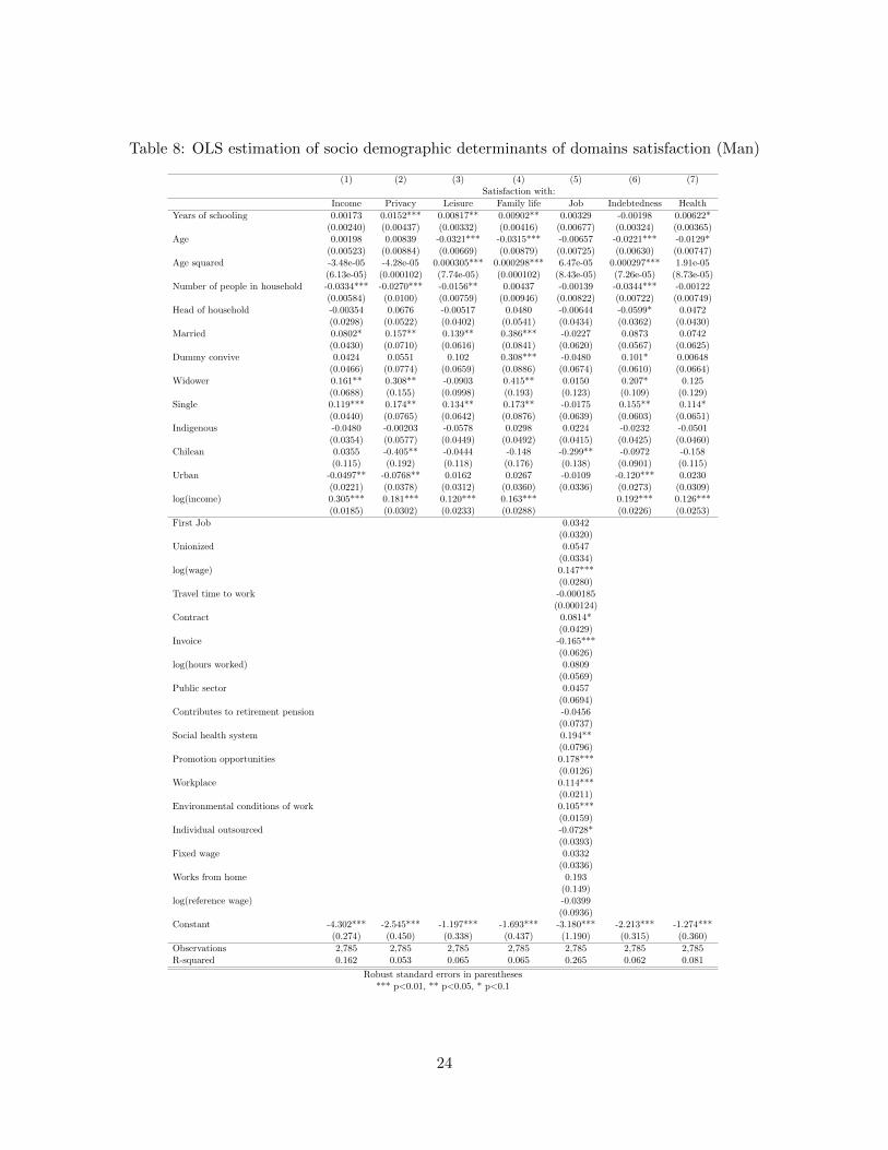
Table 8: OLS estimation of socio demographic determinants of domains satisfaction (Man)


Income Privacy Leisure Family life Job Indebtedness Health

Years of schooling 0.00173 0.0152*** 0.00817** 0.00902** 0.00329 -0.00198 0.00622*(0.00240) (0.00437) (0.00332) (0.00416) (0.00677) (0.00324) (0.00365)

Age 0.00198 0.00839 -0.0321*** -0.0315*** -0.00657 -0.0221*** -0.0129*(0.00523) (0.00884) (0.00669) (0.00879) (0.00725) (0.00630) (0.00747)

Age squared -3.48e-05 -4.28e-05 0.000305*** 0.000298*** 6.47e-05 0.000297*** 1.91e-05(6.13e-05) (0.000102) (7.74e-05) (0.000102) (8.43e-05) (7.26e-05) (8.73e-05)

Number of people in household -0.0334*** -0.0270*** -0.0156** 0.00437 -0.00139 -0.0344*** -0.00122(0.00584) (0.0100) (0.00759) (0.00946) (0.00822) (0.00722) (0.00749)

Head of household -0.00354 0.0676 -0.00517 0.0480 -0.00644 -0.0599* 0.0472(0.0298) (0.0522) (0.0402) (0.0541) (0.0434) (0.0362) (0.0430)

Married 0.0802* 0.157** 0.139** 0.386*** -0.0227 0.0873 0.0742(0.0430) (0.0710) (0.0616) (0.0841) (0.0620) (0.0567) (0.0625)

Dummy convive 0.0424 0.0551 0.102 0.308*** -0.0480 0.101* 0.00648(0.0466) (0.0774) (0.0659) (0.0886) (0.0674) (0.0610) (0.0664)

Widower 0.161** 0.308** -0.0903 0.415** 0.0150 0.207* 0.125(0.0688) (0.155) (0.0998) (0.193) (0.123) (0.109) (0.129)

Single 0.119*** 0.174** 0.134** 0.173** -0.0175 0.155** 0.114*(0.0440) (0.0765) (0.0642) (0.0876) (0.0639) (0.0603) (0.0651)

Indigenous -0.0480 -0.00203 -0.0578 0.0298 0.0224 -0.0232 -0.0501(0.0354) (0.0577) (0.0449) (0.0492) (0.0415) (0.0425) (0.0460)

Chilean 0.0355 -0.405** -0.0444 -0.148 -0.299** -0.0972 -0.158(0.115) (0.192) (0.118) (0.176) (0.138) (0.0901) (0.115)

Urban -0.0497** -0.0768** 0.0162 0.0267 -0.0109 -0.120*** 0.0230(0.0221) (0.0378) (0.0312) (0.0360) (0.0336) (0.0273) (0.0309)

log(income) 0.305*** 0.181*** 0.120*** 0.163*** 0.192*** 0.126***(0.0185) (0.0302) (0.0233) (0.0288) (0.0226) (0.0253)

First Job 0.0342(0.0320)

Unionized 0.0547(0.0334)

log(wage) 0.147***(0.0280)


Contract 0.0814*(0.0429)

Invoice -0.165***(0.0626)




Social health system 0.194**(0.0796)


Workplace 0.114***(0.0211)


Individual outsourced -0.0728*(0.0393)

Fixed wage 0.0332(0.0336)

Works from home 0.193(0.149)


Constant -4.302*** -2.545*** -1.197*** -1.693*** -3.180*** -2.213*** -1.274***(0.274) (0.450) (0.338) (0.437) (1.190) (0.315) (0.360)



24

Table 9: OLS estimation of socio demographic determinants of domains satisfaction (Woman)



Years of schooling -0.00119 0.00626 0.00177 0.00750 -0.0108 -0.00831* 0.00508(0.00367) (0.00653) (0.00527) (0.00609) (0.0107) (0.00502) (0.00570)

Age -0.0134* -0.0136 -0.0534*** -0.0217 -0.0369*** -0.0310*** -0.0285**(0.00790) (0.0138) (0.0118) (0.0144) (0.0131) (0.0108) (0.0124)

Age squared 0.000165* 0.000222 0.000610*** 0.000237 0.000482*** 0.000396*** 0.000227(9.81e-05) (0.000168) (0.000143) (0.000176) (0.000160) (0.000131) (0.000152)

Number of people in household -0.0485*** -0.0577*** -0.0302** -0.00599 -0.00291 -0.0319*** -0.0375***(0.00732) (0.0142) (0.0125) (0.0137) (0.0114) (0.0102) (0.0120)

Head of household -0.107*** -0.0712 -0.0876* -0.138** -0.0445 -0.0831* -0.120**(0.0321) (0.0584) (0.0504) (0.0581) (0.0448) (0.0439) (0.0498)

Married 0.0267 -0.114 0.0401 -0.0778 0.0115 0.0394 -0.0609(0.0473) (0.0818) (0.0669) (0.0789) (0.0628) (0.0589) (0.0693)

Dummy convive -0.0288 -0.219** -0.0483 -0.115 0.0172 -0.00471 0.0104(0.0523) (0.0959) (0.0794) (0.0885) (0.0721) (0.0732) (0.0754)

Widower 0.0768 -0.0938 -0.0197 -0.0297 0.0377 0.0947 0.316**(0.0913) (0.186) (0.125) (0.161) (0.128) (0.104) (0.133)

Single 0.0809* -0.0914 0.0814 -0.0679 0.0248 0.160*** 0.0880(0.0475) (0.0796) (0.0659) (0.0774) (0.0623) (0.0591) (0.0659)

Indigenous -0.0246 0.00968 -0.0734 0.0350 -0.0447 -0.0752 -0.0985(0.0467) (0.0778) (0.0743) (0.0755) (0.0620) (0.0618) (0.0641)

Chilean 0.129 -0.104 0.148 -0.00639 -0.0876 -0.0658 -0.150(0.147) (0.287) (0.204) (0.318) (0.164) (0.182) (0.159)

Urban -0.135*** -0.140** -0.0717 -0.1000 0.00918 -0.211*** -0.0855(0.0377) (0.0668) (0.0604) (0.0664) (0.0658) (0.0519) (0.0568)

log(income) 0.351*** 0.334*** 0.178*** 0.226*** 0.215*** 0.200***(0.0272) (0.0464) (0.0369) (0.0437) (0.0374) (0.0397)

First Job 0.0707*(0.0405)

Unionized -0.0140(0.0560)

log(wage) 0.170***(0.0422)

Travel time to work 0.000218(0.000309)

Contract 0.0348(0.0564)

Invoice -0.0880(0.0751)

log(hours worked) -0.0764(0.0728)


Contributes to retirement pension 0.0212(0.0811)

Social health system -0.0264(0.122)


Workplace 0.129***(0.0272)


Individual outsourced 0.0538(0.0653)

Fixed wage -0.0364(0.0546)


log(reference wage) 0.0744(0.119)

Constant -4.498*** -3.798*** -1.627*** -2.433*** -3.054** -2.276*** -1.776***(0.385) (0.682) (0.552) (0.678) (1.478) (0.513) (0.549)



25

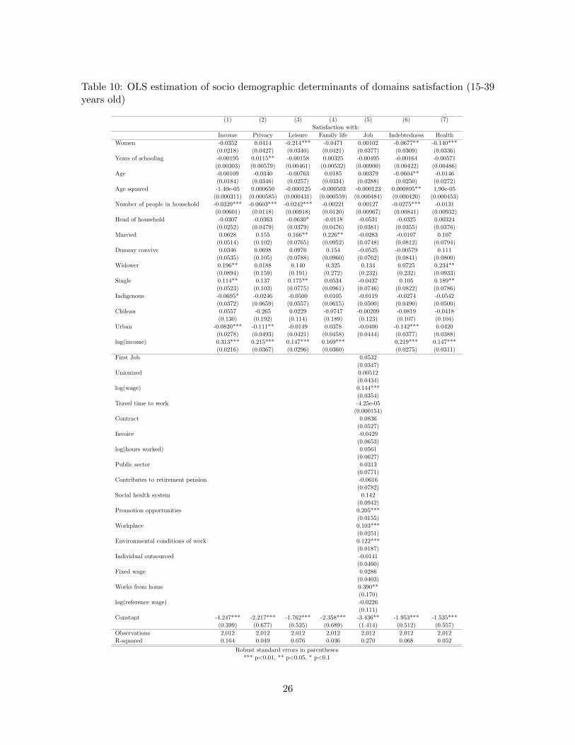
Table 10: OLS estimation of socio demographic determinants of domains satisfaction (15-39years old)



Women -0.0352 0.0414 -0.214*** -0.0471 0.00102 -0.0677** -0.140***(0.0218) (0.0427) (0.0340) (0.0421) (0.0377) (0.0309) (0.0336)

Years of schooling -0.00195 0.0115** -0.00158 0.00325 -0.00495 -0.00164 -0.00571(0.00303) (0.00579) (0.00461) (0.00532) (0.00900) (0.00422) (0.00486)

Age -0.00109 -0.0340 -0.00763 0.0185 0.00379 -0.0604** -0.0146(0.0184) (0.0346) (0.0257) (0.0334) (0.0288) (0.0250) (0.0272)

Age squared -1.40e-05 0.000650 -0.000125 -0.000503 -0.000123 0.000895** 1.90e-05(0.000311) (0.000585) (0.000431) (0.000559) (0.000484) (0.000420) (0.000453)

Number of people in household -0.0329*** -0.0603*** -0.0242*** -0.00221 0.00127 -0.0275*** -0.0131(0.00601) (0.0118) (0.00918) (0.0120) (0.00967) (0.00841) (0.00932)

Head of household -0.0307 -0.0363 -0.0630* -0.0118 -0.0531 -0.0325 0.00324(0.0252) (0.0479) (0.0379) (0.0476) (0.0381) (0.0355) (0.0376)

Married 0.0628 0.155 0.166** 0.226** -0.0283 -0.0107 0.107(0.0514) (0.102) (0.0765) (0.0952) (0.0748) (0.0812) (0.0794)

Dummy convive 0.0346 0.0698 0.0976 0.154 -0.0525 -0.00579 0.111(0.0535) (0.105) (0.0788) (0.0960) (0.0762) (0.0841) (0.0800)

Widower 0.196** 0.0188 0.140 0.325 0.134 0.0725 0.234**(0.0894) (0.159) (0.191) (0.272) (0.232) (0.232) (0.0933)

Single 0.114** 0.137 0.175** 0.0534 -0.0437 0.105 0.189**(0.0523) (0.103) (0.0775) (0.0961) (0.0746) (0.0822) (0.0786)

Indigenous -0.0695* -0.0246 -0.0500 0.0105 -0.0119 -0.0274 -0.0542(0.0372) (0.0659) (0.0557) (0.0615) (0.0500) (0.0490) (0.0500)

Chilean 0.0557 -0.265 0.0229 -0.0747 -0.00209 -0.0819 -0.0418(0.130) (0.192) (0.114) (0.189) (0.123) (0.107) (0.104)

Urban -0.0820*** -0.111** -0.0149 0.0378 -0.0400 -0.142*** 0.0420(0.0278) (0.0493) (0.0421) (0.0458) (0.0444) (0.0377) (0.0388)

log(income) 0.313*** 0.215*** 0.147*** 0.169*** 0.219*** 0.147***(0.0216) (0.0367) (0.0296) (0.0360) (0.0275) (0.0311)

First Job 0.0532(0.0347)

Unionized 0.00512(0.0434)

log(wage) 0.144***(0.0354)

Travel time to work -4.25e-05(0.000154)

Contract 0.0836(0.0527)

Invoice -0.0429(0.0653)




Social health system 0.142(0.0942)


Workplace 0.103***(0.0251)



Fixed wage 0.0286(0.0403)

Works from home 0.390**(0.170)


Constant -4.247*** -2.217*** -1.762*** -2.358*** -3.436** -1.953*** -1.535***(0.399) (0.677) (0.525) (0.689) (1.414) (0.512) (0.557)



26

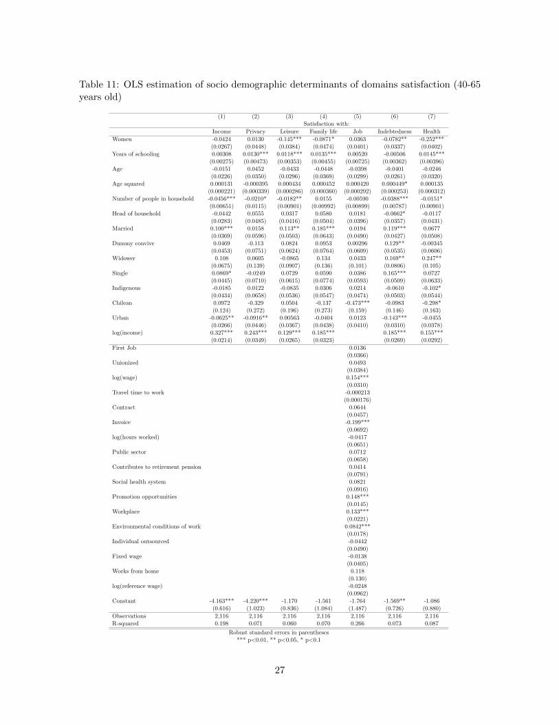
Table 11: OLS estimation of socio demographic determinants of domains satisfaction (40-65years old)



Women -0.0424 0.0130 -0.145*** -0.0871* 0.0363 -0.0782** -0.252***(0.0267) (0.0448) (0.0384) (0.0474) (0.0401) (0.0337) (0.0402)

Years of schooling 0.00308 0.0130*** 0.0118*** 0.0135*** 0.00520 -0.00506 0.0145***(0.00275) (0.00473) (0.00353) (0.00455) (0.00725) (0.00362) (0.00396)

Age -0.0151 0.0452 -0.0433 -0.0448 -0.0398 -0.0401 -0.0246(0.0226) (0.0350) (0.0296) (0.0369) (0.0299) (0.0261) (0.0320)

Age squared 0.000131 -0.000395 0.000434 0.000452 0.000420 0.000449* 0.000135(0.000221) (0.000339) (0.000286) (0.000360) (0.000292) (0.000253) (0.000312)

Number of people in household -0.0456*** -0.0210* -0.0182** 0.0155 -0.00590 -0.0388*** -0.0151*(0.00651) (0.0115) (0.00901) (0.00992) (0.00899) (0.00787) (0.00901)

Head of household -0.0442 0.0555 0.0317 0.0580 0.0181 -0.0662* -0.0117(0.0283) (0.0485) (0.0416) (0.0504) (0.0396) (0.0357) (0.0431)

Married 0.100*** 0.0158 0.113** 0.185*** 0.0194 0.119*** 0.0677(0.0369) (0.0596) (0.0503) (0.0643) (0.0490) (0.0427) (0.0508)

Dummy convive 0.0469 -0.113 0.0824 0.0953 0.00296 0.129** -0.00345(0.0453) (0.0751) (0.0624) (0.0764) (0.0609) (0.0535) (0.0606)

Widower 0.108 0.0605 -0.0865 0.134 0.0433 0.169** 0.247**(0.0675) (0.139) (0.0907) (0.136) (0.101) (0.0806) (0.105)

Single 0.0869* -0.0249 0.0729 0.0590 0.0386 0.165*** 0.0727(0.0445) (0.0710) (0.0615) (0.0774) (0.0593) (0.0509) (0.0633)

Indigenous -0.0185 0.0122 -0.0835 0.0306 0.0214 -0.0610 -0.102*(0.0434) (0.0658) (0.0536) (0.0547) (0.0474) (0.0503) (0.0544)

Chilean 0.0972 -0.329 0.0504 -0.137 -0.473*** -0.0983 -0.298*(0.124) (0.272) (0.196) (0.273) (0.159) (0.146) (0.163)

Urban -0.0625** -0.0916** 0.00563 -0.0404 0.0123 -0.143*** -0.0455(0.0266) (0.0446) (0.0367) (0.0438) (0.0410) (0.0310) (0.0378)

log(income) 0.327*** 0.243*** 0.129*** 0.185*** 0.185*** 0.155***(0.0214) (0.0349) (0.0265) (0.0323) (0.0269) (0.0292)

First Job 0.0136(0.0366)

Unionized 0.0493(0.0384)

log(wage) 0.154***(0.0310)


Contract 0.0644(0.0457)

Invoice -0.199***(0.0692)






Workplace 0.133***(0.0221)



Fixed wage -0.0138(0.0405)



Constant -4.163*** -4.220*** -1.170 -1.561 -1.764 -1.569** -1.086(0.616) (1.023) (0.836) (1.084) (1.487) (0.726) (0.880)



27

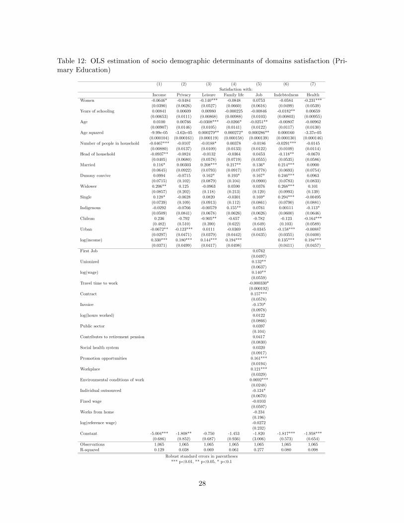
Table 12: OLS estimation of socio demographic determinants of domains satisfaction (Pri-mary Education)



Women -0.0646* -0.0484 -0.140*** -0.0848 0.0753 -0.0584 -0.231***(0.0390) (0.0626) (0.0527) (0.0660) (0.0616) (0.0499) (0.0539)

Years of schooling 0.00841 0.00609 0.00980 -0.000225 -0.00846 -0.0182** 0.00659(0.00653) (0.0111) (0.00868) (0.00988) (0.0103) (0.00803) (0.00955)

Age 0.0100 0.00766 -0.0308*** -0.0266* -0.0251** -0.00807 -0.00962(0.00907) (0.0146) (0.0105) (0.0141) (0.0122) (0.0117) (0.0130)

Age squared -9.99e-05 -3.62e-05 0.000279** 0.000272* 0.000286** 0.000160 -3.37e-05(0.000104) (0.000161) (0.000119) (0.000158) (0.000139) (0.000130) (0.000146)

Number of people in household -0.0467*** -0.0107 -0.0188* 0.00378 -0.0186 -0.0291*** -0.0145(0.00880) (0.0137) (0.0109) (0.0133) (0.0122) (0.0109) (0.0114)

Head of household -0.0937** -0.0824 -0.0132 -0.0364 0.0453 -0.118** -0.0670(0.0405) (0.0680) (0.0578) (0.0719) (0.0555) (0.0535) (0.0586)

Married 0.116* 0.00303 0.208*** 0.217** 0.136* 0.214*** 0.0900(0.0645) (0.0922) (0.0793) (0.0917) (0.0778) (0.0693) (0.0754)

Dummy convive 0.0994 -0.0715 0.162* 0.193* 0.167* 0.246*** 0.0963(0.0715) (0.102) (0.0879) (0.104) (0.0900) (0.0783) (0.0833)

Widower 0.206** 0.125 -0.0963 0.0590 0.0376 0.268*** 0.101(0.0857) (0.202) (0.118) (0.213) (0.120) (0.0993) (0.139)

Single 0.128* -0.0628 0.0820 -0.0301 0.169* 0.294*** -0.00495(0.0739) (0.109) (0.0913) (0.112) (0.0861) (0.0790) (0.0881)

Indigenous -0.0292 -0.0766 -0.00579 0.155** 0.0761 0.00111 -0.113*(0.0509) (0.0841) (0.0678) (0.0626) (0.0626) (0.0600) (0.0646)

Chilean 0.236 -0.792 -0.905** -0.657 -0.782 -0.123 -0.164***(0.482) (0.510) (0.390) (0.622) (0.649) (0.103) (0.0589)

Urban -0.0672** -0.123*** 0.0111 -0.0369 -0.0345 -0.158*** -0.00887(0.0297) (0.0471) (0.0379) (0.0442) (0.0435) (0.0355) (0.0400)

log(income) 0.330*** 0.180*** 0.144*** 0.194*** 0.135*** 0.194***(0.0371) (0.0499) (0.0417) (0.0498) (0.0411) (0.0457)

First Job 0.0762(0.0497)

Unionized 0.132**(0.0637)

log(wage) 0.140**(0.0559)

Travel time to work -0.000330*(0.000192)

Contract 0.157***(0.0578)

Invoice -0.170*(0.0978)






Workplace 0.121***(0.0329)


Individual outsourced -0.124*(0.0670)

Fixed wage -0.0103(0.0597)

Works from home -0.234(0.196)


Constant -5.004*** -1.808** -0.750 -1.453 -1.820 -1.817*** -1.958***(0.686) (0.852) (0.687) (0.936) (3.006) (0.573) (0.654)



28

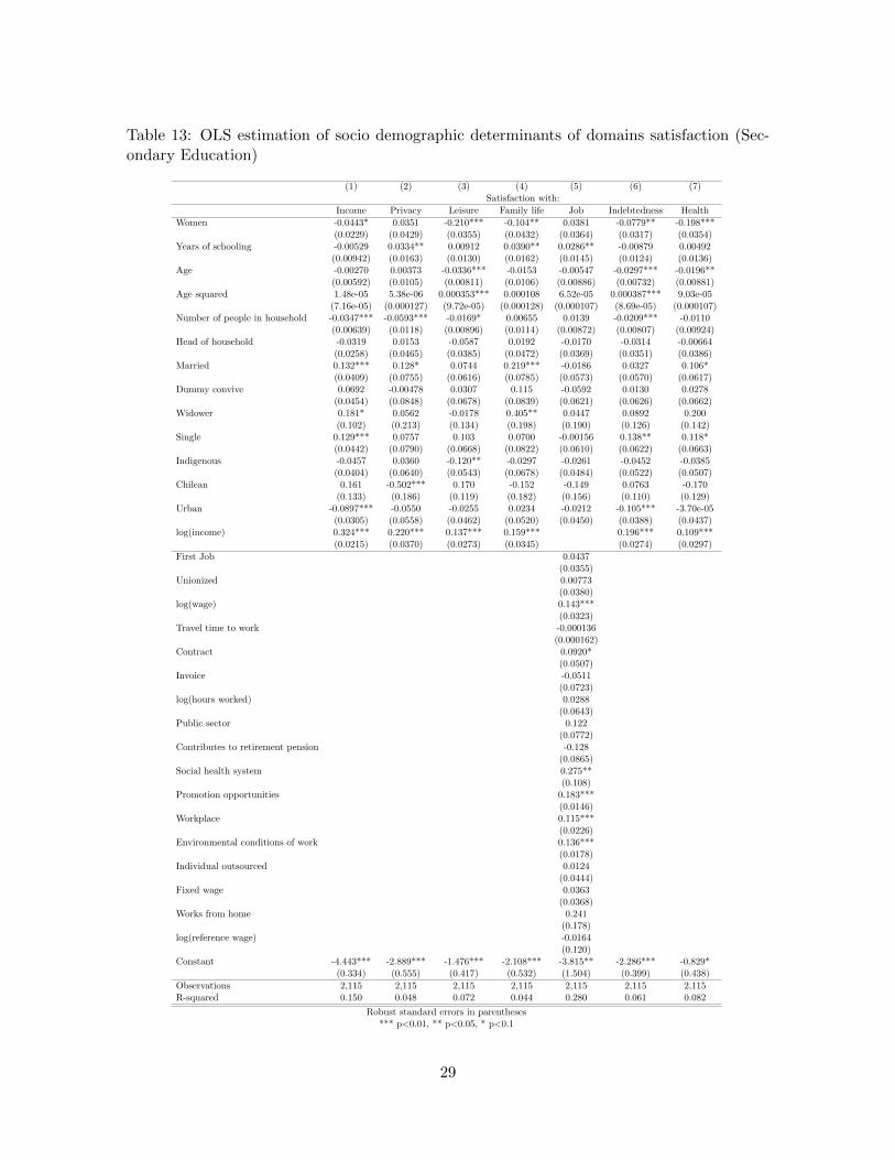
Table 13: OLS estimation of socio demographic determinants of domains satisfaction (Sec-ondary Education)



Women -0.0443* 0.0351 -0.210*** -0.104** 0.0381 -0.0779** -0.198***(0.0229) (0.0429) (0.0355) (0.0432) (0.0364) (0.0317) (0.0354)

Years of schooling -0.00529 0.0334** 0.00912 0.0390** 0.0286** -0.00879 0.00492(0.00942) (0.0163) (0.0130) (0.0162) (0.0145) (0.0124) (0.0136)

Age -0.00270 0.00373 -0.0336*** -0.0153 -0.00547 -0.0297*** -0.0196**(0.00592) (0.0105) (0.00811) (0.0106) (0.00886) (0.00732) (0.00881)

Age squared 1.48e-05 5.38e-06 0.000353*** 0.000108 6.52e-05 0.000387*** 9.03e-05(7.16e-05) (0.000127) (9.72e-05) (0.000128) (0.000107) (8.69e-05) (0.000107)

Number of people in household -0.0347*** -0.0593*** -0.0169* 0.00655 0.0139 -0.0209*** -0.0110(0.00639) (0.0118) (0.00896) (0.0114) (0.00872) (0.00807) (0.00924)

Head of household -0.0319 0.0153 -0.0587 0.0192 -0.0170 -0.0314 -0.00664(0.0258) (0.0465) (0.0385) (0.0472) (0.0369) (0.0351) (0.0386)

Married 0.132*** 0.128* 0.0744 0.219*** -0.0186 0.0327 0.106*(0.0409) (0.0755) (0.0616) (0.0785) (0.0573) (0.0570) (0.0617)

Dummy convive 0.0692 -0.00478 0.0307 0.115 -0.0592 0.0130 0.0278(0.0454) (0.0848) (0.0678) (0.0839) (0.0621) (0.0626) (0.0662)

Widower 0.181* 0.0562 -0.0178 0.405** 0.0447 0.0892 0.200(0.102) (0.213) (0.134) (0.198) (0.190) (0.126) (0.142)

Single 0.129*** 0.0757 0.103 0.0700 -0.00156 0.138** 0.118*(0.0442) (0.0790) (0.0668) (0.0822) (0.0610) (0.0622) (0.0663)

Indigenous -0.0457 0.0360 -0.120** -0.0297 -0.0261 -0.0452 -0.0385(0.0404) (0.0640) (0.0543) (0.0678) (0.0484) (0.0522) (0.0507)

Chilean 0.161 -0.502*** 0.170 -0.152 -0.149 0.0763 -0.170(0.133) (0.186) (0.119) (0.182) (0.156) (0.110) (0.129)

Urban -0.0897*** -0.0550 -0.0255 0.0234 -0.0212 -0.105*** -3.70e-05(0.0305) (0.0558) (0.0462) (0.0520) (0.0450) (0.0388) (0.0437)

log(income) 0.324*** 0.220*** 0.137*** 0.159*** 0.196*** 0.109***(0.0215) (0.0370) (0.0273) (0.0345) (0.0274) (0.0297)

First Job 0.0437(0.0355)

Unionized 0.00773(0.0380)

log(wage) 0.143***(0.0323)


Contract 0.0920*(0.0507)

Invoice -0.0511(0.0723)




Social health system 0.275**(0.108)


Workplace 0.115***(0.0226)


Individual outsourced 0.0124(0.0444)

Fixed wage 0.0363(0.0368)



Constant -4.443*** -2.889*** -1.476*** -2.108*** -3.815** -2.286*** -0.829*(0.334) (0.555) (0.417) (0.532) (1.504) (0.399) (0.438)



29

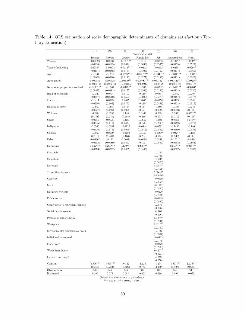
Table 14: OLS estimation of socio demographic determinants of domains satisfaction (Ter-tiary Education)



Women -0.00924 0.0503 -0.188*** 0.0112 -0.0788 -0.104** -0.183***(0.0320) (0.0625) (0.0494) (0.0633) (0.0565) (0.0435) (0.0522)

Years of schooling -0.0253** -0.00433 -0.0412*** -0.0242 -0.0192 -0.0238* -0.0293*(0.0101) (0.0188) (0.0151) (0.0192) (0.0162) (0.0137) (0.0165)

Age -0.0141 -0.0212 -0.0678*** -0.0687*** -0.0348** -0.0361*** -0.0291**(0.00930) (0.0180) (0.0141) (0.0177) (0.0153) (0.0121) (0.0146)

Age squared 0.000181 0.000327 0.000779*** 0.000787*** 0.000452** 0.000426*** 0.000295*(0.000112) (0.000216) (0.000165) (0.000213) (0.000178) (0.000143) (0.000175)

Number of people in household -0.0438*** -0.0167 -0.0345** 0.0105 -0.0202 -0.0584*** -0.0266*(0.00825) (0.0182) (0.0155) (0.0166) (0.0156) (0.0124) (0.0150)

Head of household -0.0220 0.0774 0.0197 0.110 -0.0851 -0.0562 0.0207(0.0367) (0.0710) (0.0565) (0.0696) (0.0570) (0.0487) (0.0577)

Married -0.0417 0.0229 0.0895 0.200* -0.0656 0.0129 0.0146(0.0596) (0.106) (0.0770) (0.110) (0.0851) (0.0731) (0.0915)

Dummy convive -0.0959 -0.0680 0.0154 0.137 -0.105 -0.0195 0.0246(0.0677) (0.126) (0.0956) (0.121) (0.102) (0.0973) (0.106)

Widower -0.140 -0.0193 0.148 0.0464 0.193 0.133 0.563***(0.148) (0.231) (0.203) (0.216) (0.193) (0.210) (0.196)

Single 0.0295 0.0675 0.125 0.0652 -0.124 0.0653 0.216**(0.0645) (0.118) (0.0854) (0.120) (0.0960) (0.0799) (0.0976)

Indigenous -0.0580 -0.0357 -0.0112 -0.0944 -0.0791 -0.143* -0.146(0.0626) (0.119) (0.0976) (0.0812) (0.0882) (0.0769) (0.0955)

Chilean -0.0860 0.0249 -0.0409 0.0459 -0.356** -0.297** -0.158(0.110) (0.266) (0.166) (0.284) (0.144) (0.130) (0.144)

Urban -0.0836* -0.122 -0.00881 -0.0189 0.0841 -0.170** -0.0414(0.0493) (0.0989) (0.0893) (0.102) (0.0892) (0.0703) (0.0863)

log(income) 0.347*** 0.266*** 0.179*** 0.208*** 0.256*** 0.235***(0.0273) (0.0502) (0.0405) (0.0483) (0.0387) (0.0430)

First Job 0.0359(0.0493)

Unionized 0.0345(0.0620)

log(wage) 0.168***(0.0451)

Travel time to work 5.35e-05(0.000280)

Contract -0.0919(0.0853)

Invoice -0.161*(0.0850)


Public sector -0.0888(0.0980)


Social health system -0.106(0.146)


Workplace 0.131***(0.0359)

Environmental conditions of work 0.0427(0.0304)


Fixed wage -0.0279(0.0708)

Works from home 0.430**(0.173)


Constant -3.806*** -3.065*** -0.322 -1.125 1.264 -1.853*** -1.724***(0.389) (0.783) (0.626) (0.753) (3.349) (0.528) (0.630)

Observations 948 948 948 948 948 948 948R-squared 0.196 0.073 0.083 0.052 0.239 0.099 0.079


30

Documents

Documentos de Trabajo 65 - Facultad de Economía y Empresa …economiayempresa.udp.cl/wp-content/uploads/2016/08/WP65_Montero... · Documentos de Trabajo 65 How Important is Job Satisfaction