Serie documentos de trabajo

CAPITAL ACCUMULATION GAMES

Alejandro Castañeda

DOCUMENTO DE TRABAJO

Núm. III - 1993

CAPITAL ACCUMULATION GAMES2627.

Alejandro Castaneda Sabido

EI Colegio de Mexico

camino al Ajusco N.20

Mexico, D.F . C.P 01000

Fax (5) 645 - 0464

Tel 645-0210 6 645-5955 ext . 4087

'.- ,,- .

The paper uses numerical techniques to solve an investment game with fixed costs of adjustment in discrete time . The computational teChnique uses a finite dimensional representation of the value functions for the players. The finite dimensional basis used for this approximation are bilinear cardinal functions. The model studies a dynamic game in which firms have to decide how much to invest and when to do that. The firms condition their behavior on the state of the system . The firms have to pay a fixed cost each time they want to change their level of capital. Instead of studying the entry deterrence case, the model studies a game in which given the degree of interaction, fixed costs and the depreciation rate have the right size for two firms to be active in equilibrium . In equilibrium the firms will alternate in . their investment behavior and will accumUlate capital in such a way as to delay the investment of the opponent, so that firms ar,e temporary Stackelberg leaders. The model could be use as a fully specified theoretical model that predicts alternation in market share. The model shows results reminiscent of the literature on the subject . The optimal response function when the firms decide to invest is higher for the noncooperative duopolists than for the collusive solution. Furthermore , other things being equal, the noncooperative firms wait less time to invest than the cooperative duopolists.

~ I am mostly grateful to Timothy Bresnahan and Ken Judd for very helpful comments and strong support . All errors are soley mine.

27 ·Preliminary, not for quotation.

. . , ' .

1

INTRODUCTION.

Traditionally, investment has been modelled in the industrial

organization literature' , as a strategic weapon. We can distinguish

two approaches to modelling within this literature . In the first

approach, investment is used as a tool to preclude other firms from

having a large market share. The second approach is that on entry

deterrence, 'in which the incumbent firm overinvests, installing

more capacity than it would have installed, were the threat of

entry absent . The increase in investment is designed to to deter

the potential entrant from entering the market. Representative

papers in this tradition include those by Dixit (1980), spence

(1977), Maskin and Tirole (1988 (b» and Eaton and Lipsey (1980). ' .. ,

The papers by Dixit (1980) and Spence (1977), assume a once-and-

for-all choice in the firm's level of capital. This assumption

precludes their model from being truly dynamic. The work by Maskin

and Tirole (1988 (b» supposes an alternating move environment , in

which the incumbent overinvests in each turn, in order to preclude

the other firm from entering the market. Eaton and Lipsey (1980)

analyze a continuous-time model, in which a monopolist invests

early, in order to halt the potential rival from entering the

market . Both studies exhibit rent dissipation. Firms overinvest

in order to deter the ,potential entrant from enter the market . For

Eaton and. Lipsey, the additional capital has no productive

abilities; it is used soley to deter entry. Therefore, , the

2

additional resources allocated to that ~ capital are 'w~sted. By

contrast, in Maskin and Tirole, the additional capital is employed

for, .productive uses. Assuming that firms produce at ·fuI"1 capacity,

Maskin and Tirole conclude that the addit·i'onal capital is socially

b!meficial.

A problem with this line of research lies with the fact that in the

real 'world we rarely observe a monopolist tryirig to defend its

territory against a potential intruder.

competing for market share.

Instead, we find firms

The other tradition models .. ··lnvestment as a device that prevents

other firms from increasing their market share: In their view,

firms overinvest in order to defend agairits their ' rival's

accumulation of capital. This tradition accepts explicitly the

coexistence of firms in the market .

. ··In this vein of research is the literature on irreversible

investment: Spence (1979) , Fudenberg and Tirole ' (1983). The latter

. authors studied a ' capital accumulation game with continuous

investment (over time) and no depreciationi • Spence conciudes that

speed advantages or differences in the initial conditions permit a

firm to become a .· leader and to choose a point in the follower's

optimal response function that, given the initial conditions and

', ."

They argue , that the .. assumpbi-en of zero·· depreciation allows them to highlight the importance of commitment .

. "

3

speed of investment, is closer to the s.tackelberg leader position.

Fudenberg and , Tirole find early-stopping equilibria that are

supported by the credible threat posed by firms investing until it

reaches the follower's response function.

The main goal of these papers was to emphasize the importance of

first-mover advantages in new industries.

Hanig (1986) studied a differential game in which firms invest

continuo~~ly. He uses a linear quadratic differential game. In

sharp contrast with the authors mentioned above, he allows ,for

depreciation, and bounds the level of investment by explicitly

modellIng quadratic adjustment costs. He concludes that in

comparison with the single , Cournot static Game, firms tend to

overinvest in dynamic environments. The reason is similar to that

found in Spence's model, where a firm overinvests in order to ,deter

the other firm from attaining a high level of capacity. since he

allows for depreciation to erode capital, capital looses much of

its commitment value, and, since there are no initial conditions . , ;

advantages, both firms behave 1 ike , Stackel'berg leaders. Haskin' 'and

Tirole ,(1987) reached a similar conclusion in an alternating move '

environment.

As the brief review of the literature suggests, the analyses 'of"'

investment as a strategic weapon have been unrealistic in several'"

ways. First, in some cases only the entry deterrence case has been

studied. , .. ~econd, in other cases firms were permitted to vary their , '

..

4 .. ,

stock of capital costlessly at' an~ time. 'Third, in some cases the

models were not truly dynamic. Finally, some papers assumed a zero

rate of depreciation .

I will study a dynamicc' game in which firms decide how much, and

when to invest. Firms condition their behavior on the state of the

system, which in the case of this model corresponds to the leyel of

capital of both firms. These variables are payoff relevant as

well. To formalize the idea of short run commitments, I introduce

a , fixed cost- that firms have to pay each tiine they want to change,

,their level of capital. Consequently, in equilibrium, the firms do

not ,adjust their levels of capital every period. This property

diffell"s from the ' literature ' in which firms continuously adjust

their levels of ' capital (although with some bound in the amt"' mt of

investment) (Fudenberg and Tirole (1983) and Himig (1986».

Furthermore, the inciusion ofa fixed cost endogenizes the timing

of adjustments. Also, in this modelling strategy, firms are

allowed to move any time they wish. ', These two properties are in

sharp contrast "with those of the alternating move approach (Maskin

and Tiro-Ie's models (1987); (1988 (b».

Like Hanig, I will study a: capital accumUlation game which allbws

for depreciation. In contrast with Maskin and Tirole's study (1988

(b», given the degree of interaction, in my work the fixed cost is

small enough, and the rate of depreciation small enough, to allow

both -firms to be act:i\,e in " equilibrium . . "

Instead of deterril;lg

•

5

entry, the firms accommodate each other.

An interesting question emerges in this context. Given the

permanence ,of the competitor in the industry, under what conditions

can a firm take advantage of the sluggishness in competitor's

response, and delay th~ rival's inv~stment in order to establish

itself as a temporary Staekelberg leader? The main goal of ' this

paper is to answer this question.

The primary contribution of this work lies in building a model

where investment is a strategic weapon, and which entails more

. realistic assumptions re<;jarding the competitive process1 • The

resul,ts are ,reminiscent of the previous literature on · the subject.

Instead of. having entry deterrence, or permanent Stackelberg

leadership, we obtain results in which firms alternate in their

investment behavior, and accumulate capital in such a way as to

delay the investment of the opponent, so that firms are temporary

Stackelberg leaders. Because the rate of depreciation is positive,

there are no first mover advantages . Rather, if we are willing to

maintain the assumption that firms produce at full capacity, the

model studied here could be considered a fully specified theory

that explatns the alternation in market share among firms.

. . ..;

1 Fixed costs of adjustment, positive rate of depreciation, co~xist~nce . of few firms in the market and the analysis of , a truly dynamic inodel.

6

Section 1 states" the ' basic ,assumptions of the model. I -'argue that

the one period return function involves a model in which capital

~ffects marginal cost, and price competition is subsumed in the

. IIlQdeL.

section 2 states the dynamic setting and presents the pair of

functional equations that has to be satisfied in order for the \

model to be a Markov Perfect Equilibria. I also sketch the main ....... '

computational approach3 • Section 3 presents the parameter values

chosen to solve the model. Section 4 states the results of the

game. Because the one period return function exhibits the property

of strategic substitutes, the firms will never choose to adjust

their state variables at the same time ; I also look at the play

set, the set of states in ' which , the firms will stay after the

initial move. The set shows an area of ,'mu'ltiplicity of eqUilibria

in ,which we have two types. of equilibria. If one firm invests;

then it is optimal for the . rival to stay put. However, if the

first firm decides to stay . put" then it is optimal for the rival to

invest. Theresul·t . is not :surprising given the property of .. ,; .

strategic substitutes that the return function exhibits.

In section 5 I perform comparative statics analysls with respect ' to

changes in the parameters of the model. In section 6 I highlight

an important result that appears to be persistent for all models;

3 Appendix .. one has ,a mor,e detailed.; explanation of , ' the computational approach.

7

0, for some states, a firm will wait until the competitor is about to

move, and in the period before, it invests in order to further

delay the adjustment of the competitor. I call this phenomena

"partial preemption" and the result is reminiscent of the Eaton and

Lipsey's (1980) conclusion.

In section 7 I , change the degree of interaction', and see how the

firm's investment pO'licy responds to these parameter ' changes.

" Given the partial ' preemption result, we see that for higner' degrees

-,~; ' of interaction the firms invest less frequently.

In Section 8 I make comparisons with the collusion case. I

.,.' conclude that for higher degrees of interaction, ' the two product

monopoly will adjust more frequently than the oligopolistic firms.

For low degrees of interaction we get the opposite result.

However, even in the latter case, firms attain higher levels of

investment (each time that they decide to invest) than in the

collusion solution. Firms will invest beyond the monopolist level,

a result reminiscent of the former literature, and of the

traditional static Cournot analysis.

Finally in sec·tion 9 I make a welfare analysis. I find that the

.. -',. , , ' social planner adjusts her capi tal more frequently ·"than the

., oligopolistic ' firms. This is because the firms '"willl "follow

policies of "partial preemption", which allow them to become

temporary Stackelberg leaders, and delay the adjustment of the

:

-'

8

competitor as much as they can. We will also see that changes in

the rate of depreciation affect negatively the present value of the

producer surplus.

i.'.· ..

;:;-'.~ _. ".:

j:~ ' .'

. . . ' .... . -;

. ~.

9

1. THE MODEL Consider an industry with two symmetric firms with th~ return

function expressed in terms of capital This return

function4, F'(o, o) i-l,2 , is strictly concave, so that for each level

of capital of the rival firm , we have a well defined optimum for

the first firm. Finally, I assume that F,'. (x., x.) <0 i-l,2 , Le. it

exhibits the property of strategic substitutes.

Each time a firm wants to invest in new capital , it has to pay a

fixed cost K , which is the same for both firms. The fixed cost

will force the firms to be inactive during some time. A salient

feature of this model is that it determines endogenously the time

of investment by the firms, as well as, the size of the investment . .'

1.1 PROFIT FUNCTION. I study a game with the following quadratic' profit function :

.,

Following Fudenberg and Tir ole (1983) , I assume that the profit

function is the reduced form of a pr ocess in which firms compete in

prices . I aSsume in (1) that firms choose prices in a world of

imperfect SUbstitutes such that they produce at full capacity •

Below, I address the appropriateness of .. this assumption. We notice

immediately that nt2(o,o)<0 , since O<DB<l , Le . the profit fU]lction

has the pr operty of strateg ic sUbstitutes . DB has also the

function of parameterizing the degree of interaction. The property

4 See the next SUbsection .

10

of strategic sUbstitutes implies that larger levels of the rival 's

capital, decreases the marginal profitability of capital for a

ftrm. . . Given the endogeneity of the decision to 'invest in this

model, this property should imply that firms will not adjust their

capital at synchronous times. Rather, given that the rival has

already invested, it may be optimal for a firm to stay put for some

time. Indeed, this is one of the main results of the paper.

Equation (1), was obtained by calculating the inverse ' demand

£unctions obtained by the maximization of the following utility

function:

(2)

Equation (2) ' posits a representative consumer, DB represents the

degree of substitution bEi'tween goods. I calculate the demand .,.

functions from the utility function in (2) To obtain equation

(1) I solve for the inverse demand function and substitute it

into the profit function of eaoq, firm. The reader may wonder why

I use an imperfect substitute model to analyze quantity

competition; indeed, the optimal response functions are continuous

in the traditional static Cournot model, in which goods are perfect

sUbstitutes. For the imperfect sUbstitute case, the social , ...

planner and the collusion solution, gives me an. independent choice

for the levels of capital of each of the two firms. In the perfect

sUbstitute case',. the social 'planner and the collusion model will

only give me a solution for the total level of capital of both

firms (the sum of capital for both firms), leaving undeterminate

11

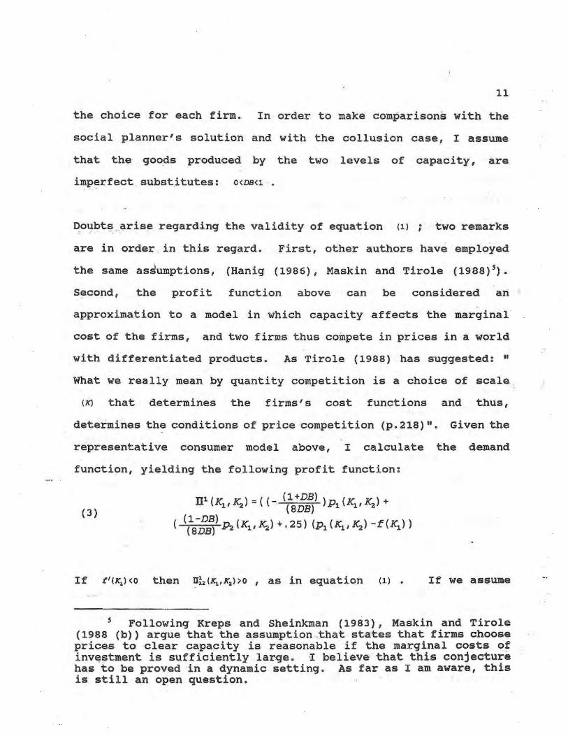
the choice for each firm. In order to make comparisons with the

social planner's solution and with the collusion case, I assume

that the goods produced by the two levels of capacity, are

imperfect substitutes: O<DB<l '

Doubt~ , arise regarding the validity of equation (1) ; two remarks

are in order . in this regard. First, other authors have employed

the same as~umptions, (Hanig (1986), Maskin and Tirole (1988)5).

Second, the profit function above can be considered art

approximation to a model in which capacity affects the marginal '

cost of the firms, and two firms thus compete in prices in a world

with differentiated products. As Tirole (1988) has suggested: "

What we really mean by quantity competition is a choice of scale ,

(~ that determines the firms's cost functions and , thus,

determines the conditions of price competition (p . 218)" . Given the

representative consumer model above, I calculate the demand

function, yielding the following profit function:

(3) D'(IC ~)=((_(l+DB»p (IC ~)+

1"'2 (8DB) 1 1'"'2

(l-DB) (8DS) ~ (K

" K2) + • 25) (P, (K

" K2) - f (K, ) )

If f'(K,) <0 then D~,(K,.K,»O, as in equation (1,). If we assume

5 Following Kreps and Sheinkman (1983), Maskin and Tirole (1988 (b» argue that the assumption .that states that firms choose prices to clear capacity is reasonable if the marginal costs of inv~stment is sufficiently large.! believe' that this conjecture has to be proved 'in a dynamic setting. As far as I am aware, this is still an open question.

12

that the function f'(K,) is linear then the profit function is

quadratic. However, the function is not concave in ~ . In order

to employ this profit function in my dynamic model I would need to

' assume a quadratic cost , of adjustment in the level of investment,

which is ' a property that exponentially increases the number of

calculations6• One way to circumvent this problem is to assume that

the ·'function f'(K,) ' is nonlinear with locally increasing returns,

and asymptotic decreasing returns. This assumption bounds the

choice ~ in the one period return function. However, the return

function would no longer be quadratic . If we were to consider the

true profit function in this setting, I believe that the results

would not significantly vary from my specification. I consider the

profit function in equation (1) as an approximation of the true

profit function in equation ' (3) , with nonlinear f'(K,) 7

6 See chapter two.

7 This assumption has been widely used in the macroeconomics literature. For example, Christiano (1990) and Hansen and Sargent (1990), assume that a quadratic function is a good approximation of more general nonquadratic functions.

13

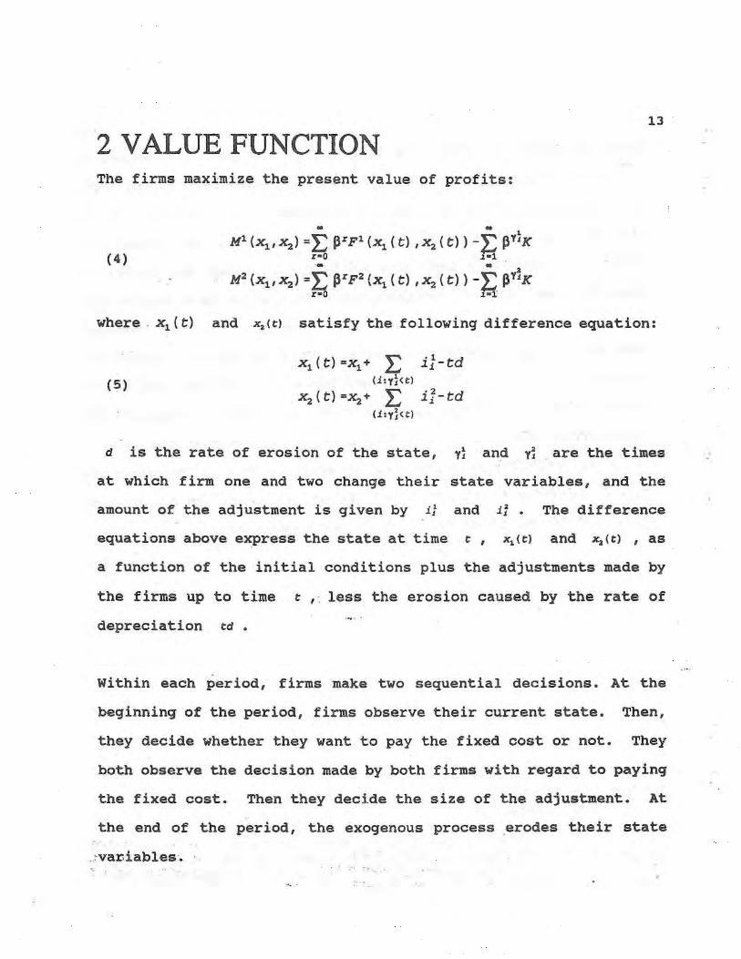
2 V ALUE FUNCTION The firms maximize the present value of profits :

• •

(4)

, Ml (Xl ,X2) =E ~rFl(Xl ( t) 'X2 (t» - E ~Y'K

x-o ~ -1 . '. . , M2 (Xl , X2) =E ~rF2 (Xl ( t ) ,x, ( t» - E ~Y'K

x-O ~·l·

where , Xl ( t ) and x,(e) satisfy the following difference equation:

(5)

Xl(t ) =Xl + E iJ-td (j:yl<t)

x 2 (t) =x2+ E iI-td (1ly~<t)

d is the rate of erosion of the state, yl and yj , are the times

at which firm one and two change their state variables, and the

amount of the adjustment is given by i; and it. The difference

equations above ex,press the state at time e, x, (e) and x, (e) , as

a function of the initial conditions plus the adjustments made by

the firms up to time t , c less the erosion caused by the rate of

depreciation ed .

within each period, firms make two sequential decisions . At the

beginning of the period, firms observe their current state. Then,

they decide whether they want to pay the fixed cost or not. They

both observe the decision made by both firms with regard to paying

the fixed cost. Then they decide the size of the adjustment. At

the end of the period, the exogenous process ,erodes their state

.. ,var-iables:. .. . . ; .

...

. " .

14

For· each . period, firms play a two stage game. This game's

extensive form is! depicted in Graph 2.1. and the corresponding

normal form is expressed in Graph 2.2. As we can see from the

extensive form, there may be mixed strategies involved in the

decision of whether to pay the fixed cost or not. The p in the

following functional equation (10), represents the probability

that firm one pays the fixed cost in that period.

the probability that firm two pays the fixed cost .

q represents

s' in (10)

is the optimal response function of firm one. Due to the linearity

of · the cost adjustment function, it is function of · the current ,

state for firm two (x,) . if two does not move. If two does move,

then s' corresponds to the intersection of ·the optimal response

functions. A similar explanation holds for firm two.

Let V'(x, .x,) i-1.2 be the value function associated with. a Markov

Perfect Equilibria S!olution , S!tarting at time 0 with capital

The value function of both players is defined by the

simUltaneous solution of the following pair of functional

equations:

(6 )

Vl (Xl' X2) =Max p [qMax[F l (Sl, S2) +BVl (sl-d, s2_d) -Cm (Sl_x1 ) 1 P, 51

+ (l-q) Max[Fl (Sl, X2) +BVl (Sl-d, x 2-d) -Cm (SLX1 ) 1 -K] s'

+ (l-p) [q[F l (Xl' s2) +BVl (xl -d, S2-d) 1 +

(l-q) [Fl (X1,X2) +BVl (x1-d,x2-d) II =TV1

V:. -(X1, X2) =Max q[pMax[F2 (Sl, S2) +BV2 (SLd, S2-d) -C",(SLX2 ) J q, sa

+ (l -p) Max[F2 (Xl' S2) +BV2 (Xl -d, S2-d) -Cm (S2_ X2 ) 1 -K] s' +(l-q) [p[F2 (Sl ,X2)+BV2(Sl-d,x2-d)l + (l-p) [F2 (X1'X2) +BV2 (xl -d,x2-d) II =TV2

15

~ . ,

A Feedback Nash equilibria is a quadruple (p,S';q,S') , so that both

equations in (6) are satisfied.

I define Oc as the set of '" and x, in which 'it is an .'

equilibria that neither of the firms wants to move, p and q are

equal to zero in (6) • Alternatively, 0, is the set of states in

which only firm one wants to move, p is equal to one and q is

equal to zero in (6) above. When p is equal to zero and q is

equal to one then the firms are in the set 0, If p is equal

to one and q is equal to one, then the firms are in the trigger

set for both firms 0., whenever firms are in this set they move

to the intersection of the optimal response functions S'(Xj).

Finally, I obtain the set in which p and q are between one and

zero. This set contains mixed strategy equilibrium. Let me call

this set 0_. s'(X,) represents the low boundary between the

trigger set for firm one and the continuation set when the state of

16

firm two is at ~ 8 • Finally, s represents the point at which

firm one (and firm two) decides to move whenever both firms ' are

moving together .

. '( '.

If the extensive form of the game for each period is not .. defined in

this way, every time in which there is not a consist.ent .outcome in

pure strategies, I would have had a very difficult task in \

calculating the mixed strategy equilibria. This is so, because the

action space is continuous' . The fact that firms observe whether

they have paid the fixed cost in the first stage of the period,

allows me to restrict the strategies upon which firms can

randomize. In this setting, the mixed strategy . equilibria occurs

only when firms have not a consistent decision in pure strategies

about paying a fixed cost .

We can view the right hand side of the equations in (6), as an

operator which maps tomorrow's value function into today's value

function. If the solution exists, (see the paragraph below) the

standard procedure for solving the pair of functional equations

expressed above is to start with an arbitrary function and to

iterate in the fOllowing .~ap until convergence is reached· . .... . ;

8 since capital can° be reduced and increased, there is a high boundary between the continuation set and the trigger set for each of the two firms. But, because depreciation is a one sided process these wiH. never be attained after the., second m(Jvement.

9 ~ven in the case of discrete action spaces it is impossi6ie . to calculate- the mixed strategy equilibria in the computer,

··whenever firms are mixing between sevenll possible choices.

:' , ';. "

r .J ..

17

(7)

In the single decision case with standard assumptions on the one

period return function F ' (',') and the discount factor B, the

·· .. contraction mapping theorem guarantees the convergence of the

iteration in (7) • Obviously , existence for strategic environments

is not a simple extrapolation of this argument.

I am not aware of an existence proof for this type of games . Dutta

and Rustichini (Dutta and Rustichini 1991) have proved existence in

a game similar to this one , but with one state variable10 II. We

have existence theorems for games with discrete ' state space and

controls restricted to points i n the grid (Fudenoerg and Tirole

(1991), chapter 13 theorem 13.2).

Existence from a computational perspective is verified by seeing

whether the approximation in the computer is actually converging.

As Judd (Judd 1990 (b)) has suggested , the computational approach

to these models may be viewed as an analogous procedure towards

10 Since the optimal response, function is non-convex, Le. for some states thEb player does pot lIlove., a"d for others she does . Traditional existence results which rely on the Kakutani Fixed Point Theorem cannot be used. The Dutta and Rustichini's method uses some kind of monotonicity in the optimal response function,

:1 ,·, ; .. ~ and then, they use Tarski fixed point theorem to prove existence . ,. ,.... I suspect that this approach may work for this model.

,. i

II Existence of the open loop equilibria is no problem. Once the other firms strategy is chosen, the opti mization problem

d " becomes a single agent procedure. In continuous time, the proof of ' a existence of an optimal policy for a single decision maker would

apply (Bensoussan and Crouhy (1983)).

18

.proving existence. The. computational soluti;on may be"thought of as

an epsilon equilibria of the original problem.

Given . the f ,act that I solve the model in the computer in discrete

time, differentiability cannot be guaranted for the whole state

space. In par.ticular, the value function is not differentiable at

the boundary be~ween the continuation set and the trigger set. The

fact that a firm can either decide to wait for a period to adjust,

or instead adjust right now, implies two different control choices

for that firm. It can wait one period to exert its control,

thereby choosing implicitly a discretely lower state variable for

tomorrow. Alternatively, it can exert its control without delay

and qhoose a higher value of the state variable for tomorrow •

. .. ,S:,learly, this implies that the value function is not differentiable

. ~t any boundary between the continuation set and any of the trigger

sets. Moreover, for all initial states in the continuation ' set

that hit the boundary exactly, the value function remains

nondifferentiablel2 • This las,t reasoning insinuates that the value

function is only piecewise differentiable in discrete time.

Consequently, it is important to keep our approximation in a ' space

suitable for these properties of the value function. A ' similar

proof to the one made in castaneda · (1992 (a» in continuous time,

will show that the value function is continuous in discrete time •

. ; -.

12 See" Lucas and stokey (1990) page.11B for an example that shows this particular problem. ' ".

19

In appendix one I explain more carefully the computational

approach, here, I only sketch the main procedure. Given the

theoretical restrictions analyze.g so far, it is natural to look for

value functions in the space ~ of piecewise differentiable

.. ... "functions mapping DcIII' into .' since the computer cannot

.; ~

approximate the whole space of piecewise differentiable functions,

I look for a finite dimensional representation of the value

function 13

I calculate the mapping T in (7) in two stages.

First, I solve 'for the Nash equilibria in a square lattice '·with

equally distan't''. 'points in both dimens'ions so that T is exactly

satisfied in . (1) 'for any point in the lattice. Any point in' the

lattice is given by the following ordered pair: Where ~.

x,-c;+ih' i-O,99 and Xj-c;+jh j-O,99. Furthermore, the origin of the

lattice is on the forty five degree line so that ~;-cl 1.... Second,

I seek for an interpolation method . that best satisfies the ..

theoretical restrictions of the model, and that better summarizes ,.

" the information obtained from the points of the lattice. By using

this procedure, I replace the theoretical mapping from the space " " i~ lJ

of continuous functions into continuous functions represented in

(7) by T, into a finite dimensional ' approximation of that map.

13 Judd (1990) is a very good paper on computational approaches in economic analysis. The impact of that paper in this part of this chapter is considerable.

14 In general c;-cl were very close to zero, so that the whole grid was in the positive orthant.

:

....

20

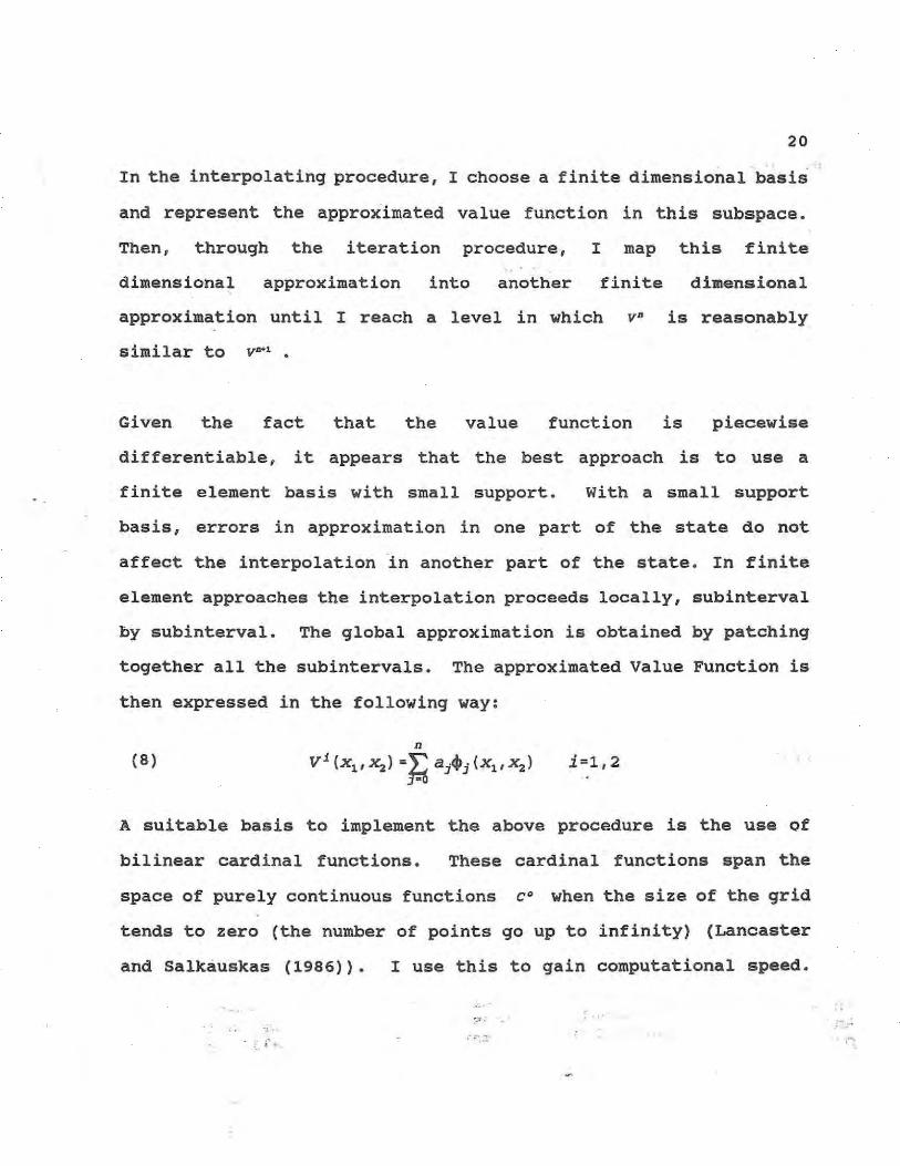
In the interpolating procedure, I choose a finite dimensionalb·~sis '

and represent the approximated value function in this subspace.

Then, through the iteration procedure, I map this finite

dimensional approximation into another finite dimensional

approximation until I reach a level in which v· is reasonably

similar to V"'.

Given the fact that the value function is piecewise

differentiable, it appears that the best approach is to use a

finite element basis with small support. with a small support

basis, errors in approximation in one part of the state do not

affect the interpolation in another part of the state. In finite

element approaches the interpolation proceeds locally, subinterval

by subinterval. The global approximation is obtained by patching

together all the sUbintervals. The approximated Value Function is

then expressed in the following way:

(8) i=1,2

A suitable basis to implement the above procedure is the use of

bilinear cardinal functions. These cardinal functions span the

space of purely continuous functions co when the size of the grid

tends to zero (the number of points go up to infinity) (Lancaster

and Salkciu·skas (1986)). I use this to gain computational speed.

~ ... ,: .. '

-""0' : t. ·

. ,""\

21

Bilinear cardinal functions are easy to constructu .

15 This argument is not true for higher order approximations. In such case the cardinal functions may have to be calculated. And when we calculate them, they may not have the small support property.

22

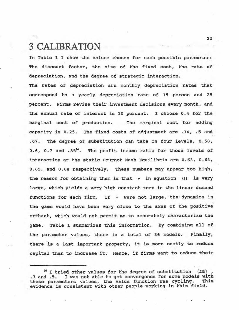
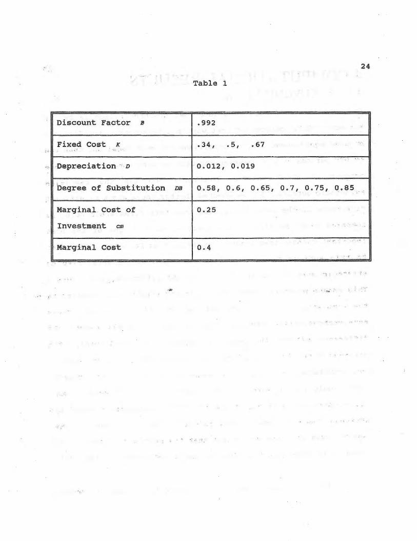
3 CALIBRATION In Table 1 I show the values chosen for each possible parameter:

The discount factor, the size of the fixed cost, the rate of

depreciation, and the degree of strategic interaction.

The rates of depreciation are monthly depreciation rates that

correspond to a yearly depreciation rate of 15 perc en and 25

percent. Firms revise their ,investment decisions every month, and

the annual rate of interest is 10 percent. I choose 0.4 for the

marginal cost of production. The marginal cost for adding

capacity is 0 . 25 . The fixed costs of adjustment are .34, .5 and

.67 . The degree of sUbstitution can take on four levels, 0.58 ,

0.6, 0.7 and .8516• The profit income ratio for those levels of

interaction at the static Cournot Nash Equilibria are 0.63, 0.63,

0.65. and 0.68 respectively. These numbers may appear too high,

the reason for obtaining them is that v in equation (2) is very

large, which yields a very high constant term in the linear demand

functions for each firm. If v were not large, - the ' dynamics in

the game would have been very close to the axes of the positive

orthant, which would not permit me to accurately characterize the

game. Table 1 summarizes this information. By combining all of

the parameter values, there is a total of 36 models • Finally, .....

there 'is a last important property, it is more costly to reduce

capital than to increase it . Hence, if firms want to reduce their

16 I tried other values for the degree of sUbstitution (DB) , .3 and .5. I was not able to get convergence for some models with these parameters val~es , the value function was cycling. This evidence is consistent with other people working in this field.

;.

23

level of capital, they will have to pay an extra fixed cost equal

to 0.25 .

, .

"

. , ..

24

Table 1

Discount Factor B .992

Fixed Cost K .34, .5, .67 ' . . ' "'

" .

,Depreciation ·'· D 0.012, 0 .019

Degre'e of substitution DB 0.58 , 0 . 6, 0 . 65, 0.7, . 0 .75, 0 . 85 . ,

Marginal Cost of 0.25

Investment em .. ..

.. ~. .. .", - .

Marginal Cost 0.4 . , " ..

--. '~ : ' . "' ., .' >

. . : . ...... ,

.: :.

4 COMPUTATIONAL RESULTS. 4.1 SYNCHRONIZATION.

25

In Castaneda (1992 (b» is argued that synchroriization is by far

the most robust outcome of that work's simulations. I select one

hundred equidistant initial conditions for each model and then run

10,000 periods ina simulation for 'each initial condition. In this

proc~ss, I check whether synchronization was the resulting

asymptotic outcome. I also checked whether there was a significant

difference in the level of capital that both firms would hold, as

compared with the size of the inaction setl7 • One of the most

important changes that I make in passing from Castaneda (1992 (b» ,,'

to ,this work is the switch from ' strategic complementarities to

strategic SUbstitutes in the one period return function 11(00 0) •

This change produces completely different results with respect to

the simulations. For all models and for all initial conditions

non-synchronization was the only outcome. In all cases, the

difference between the level of capital was significant, when

compared with the size of the set of inaction. Additionaly,

synchronization in capital adjustment is an unstable process.

Firms would rather invest in new capital in asynchronous times .

Villas-Boas (1990) obtains a similar result in a model in which the

strategy space is considerably reduced. The intuition for this

result ,comes from the assumption that the profit function has the

property of strategic sUbstitutes. We remember that in the static

17 The continuation set in the terminology of chapter two.

26

Cournot case with strategic substitutes, the optimal response

function is negatively sloped. The higher the rival's quantity

(capital), the lower the quantity (capital) that the firm wants to

have. In this model, the intuition of the static Cournot model- is translated into the following: If the rival wants to have a higher

level of capital, it is optimal for the first firm to maintain its

level of capital at a lower level. In the next section we will see

that therei~ an area of the state space in which it is optimal for

a firm to invest if the rival wants to stay put, but would rather

stay put if the rival wants to invest. The reason for · the

existence of this area follows the same intuition. Therefore, if ... .......... .

the rival firm wants to invest now, it is optimal for the first

firm to stay put and to maintain a low level of capital.

The inclusion of a fixed cost of adjustment introduces a a new

dimension in the analysis of capital accumulation games. In Maskin

and Tirole's model (1987), as well as in Hanig's model (1986),

symmetr ic firms maintain the same high level of capital in the

steady state (i.e. both firms behave like stackelberg leaders).

When we include a fixed cost in the analysis, the equilibrium

behavior changes radically. Both firms alternate their levels of

capital and the levels of capital are never equal between the

firms. '. "-

27

4.2 PLAY SETI8.

Graph one illustrates the different sets for the state space. In

all models I noticed that there is a large set of states that yield

multiple equilibria . Firm one will move only if the other firm .

does not move, and will stay put if the other firm moves. Given

the method of solution proposed above-Le o to flip a coinI9_, the

firm' that moves adjusts its capital up to the optimal response

function. This result is not surprising, given the assumption of

strategic substitutes. Both firms seek to preempt the rival, but

if one randomly gets to move first, then the other firm would

rather stay put. ' As mentioned in the last section, the intuition

for this result follows from the slope of the optimal response

function of the static game with strategic sUbstitutes. The higher

the rival's capital, the .lower the level of capital that a firm

wants to have. In the context of this model, the intuition is as ,

follows: If the rival wants to invest and therefore have a higher

level of capital, the firm would prefer to maintain a low level of

18 We can define the play set as the set of states in which the g<!.me will be played after the second move. Some of these states may be visited only very few times, whereas' others will be frequently visited. By looking at the shape of the state and the simulation results, it seems that for the case with strateqic . substitutes firms will visit more states more often than in the case with strategic complementarities (see castaneda (1992 (b» . The reason for this result, is that synchronization is locally stable for the strategic complements case, whereas is locally unstable for the strategic substitutes case.

19 By flipping a coin, I capture idiosyncratic shocks to any firm that permits the other to preempt it.

28 . ~

capital. ThtsI'esult impl!:i.e~ that synchronization is locally

unstable. For . reference I will call this set 0 •.

If we look at graphs one and two we will see that 0. is far ..... . . larger for higher degrees ' of ·interaction (graph one corresponds to

DB- . 58 , and graph two corresponds to DB-.8S ). Given the fact· that

firms are strategic substitutes, for higher degrees of interaction

there are more states in which both firms seek to preempt the

rival. Any negative exogenous shock that affects a firm will prove .

advantageous for the other firm, since the shock allows the firm to

invest, and preempt, at least temporarily, the rival.

It is interesting to analyze the shape of a typical response

function S'("1) for a firm that decides to move. For states close

to the trigger set of ':he other firm °1 , the optimal response

function is increasing. This is because the firm that moves (i)

is aware that the rival will move, within a short period. Given

the fact that capital is a strategic sUbstitute variable, it would

rather move to a lower level, the closer the time for the rival

(j) to move. As we get further away from the trigger set of the " ~" '"

other firm °1 , the optimal response function S'("1) becomes

negatively sloped as in the static cournot case. . The reason is the

traditional Cournot explanation: the higher the other's firm

capital, the lower the new level of capital that the firm that is

moving wants to have. These properties of the optimal response

function appear to be valid for all models. Again, as we shift

29

from a higher degree of interaction (graph one), to a lower degree

(graph two), the optimal response function moves down. If the

degree of interaction is high, the firms will behave more like

stackelberg leaders whenever they decide to move. The higher the

degree of interaction, the higher the level of investment that the

firms want to maintain .

. . ~

.5 COMPARATIVE STATICS 5.1 INCREASE IN THE FIXED COST

30

The size of the play set increases for both levels of depreciation • ..

Further, s' (Xj) the optimal response function goes up, and B' (xj )

the boundary between the trigger set and the continuation set for

each firm goes down, this property holds true for both levels of

depreciation . Graph three illustrates these results.

Regarding simul"ations20, I obtain the following results: The

frequency of capital adjustment decreases as the size of the fixed

costs increases . This happens for both levels of depreciation, for

all values of DB, and for all the changes between K-.34 and

" K-.5 , and between K-.5 and K-.67 (See Table 2) .

5.2 INCREASE IN THE RATE OF DEPRECIATION

When the rate of depreciation increases the size of the Play set

goes up for all values of DB s' (Xj) , the optimal response

function, goes up as the rate of depreciation goes up for all "

values of the fixed cost, and for all values of degree of

interaction . B'(Xj) I the boundary between the trigger set for any

of the firms C, and the continuation set Cc drops, again this "is

" , 20 As I explain below, for each initial condition and for each model in the simulations, I count the number 6f adjustments in the level of capital that the firms make. This measure' gives me an idea on how frequent the firms adjust capital.

31

true for all fixed costs, and for all values taken on by the

degree of interaction. Graph three illustrates these results.

For the three levels of the fixed cost K- . 34, K-.5 -and K-.67 and ,

for ~ll level~. oJ the, degree of interaction DB, we find that an

in the rate pf depreciation increases the frequency of capital

adjustments (See Table 2).

6 PARTIAL PREEMPTION

It is worth highlighting a result that appears to be persistent for

all models. If we look closely at Graph one we will notice that,

in the boundary between _ the continuation set and the set of

multiple equilibria 0.. (the small white squares), there are

states in which only one firm moves. The result is reminiscent of

the literature on Preemption by Maskin -and Tirole (1988 (b» and

Eaton and Lipsey (1980). A firm adjusts its capital just before

the oth~r firm is about to be interested in moving, and in doing

so, adjusts to the highest level of capital that it is possible in

the game. This tactic allows the firm to succeed as a temporary-

"stackelberg" leader, at least until the other firm reaches the

boundary between its trigger set and the continuation set. Given

the property of strategic substitutes, the firm adjusting its

capital delays the increase in the capital of the other firm until

the firm that was preempted has such a low level of capital that it

decides to increase. If we look carefully at graphs one and two,

,. ".

· ,; r ~. !L' ~'.:-" , ' .. ' i' ...... ~ .. \ ":-: ' .~~.'~i <'·,il·

, ,

32

we notice that the area of preemption is larqer for higher degrees

of interaction. This happens because the area of multiplicity

Q_ I ' ,i$ , larger for , higher degrees of interaction. Furthe~ore, l

for higher degrees of interaction, " the area of preemption is

locat~d at higher levels of the state than for lower degrees. The

intuition , here is straightforward, s'ince for higher degrees of

interaction, firms will wait less time to preempt their rival .

7 CHANGES INTERACTION

IN THE DEGREE OF

In Table 2 I report the average number of adjustments in the level

of capital made by a firm. The method of calculating these numbers 1. ," <.\ :-

is as follows . As ,stated in s'ebtic'in 4.2 : l ' I selected one hundred

equidistant-initial condition for each parame'ter model. Then I

simulated 10,000 periods for each initial condition and for each

parameter model. In this process I count the number of adjustments

that the firms make. The numbers indicate an average over the one

,hundred' ini tial conditions for each set of ' para!l)eter values21• We , '

note tHat, ' as 'the' 'degree of interaction increases, the average

number of ' 'adjustinents decreases. The reasons for this are twofold.

On' ,the omf hand, by looking at graphs one and two, we note that the

optimal response ' function is higher for higher degrees of

21 The standard deviation of the average number of adjustments was in all cases extremely small," so that the average is a good indicator of the number of adjustments for , each model.

33

interaction. caeteris paribus, this fact implies more time between

adjustments. At the same time, the boundaries between the trigger

sets for both degrees of interaction are almost at the same level.

The second reason comes from the idea of "partial preemption". In

graph one we see (using the arrows), that firms delay the

competitor's adjustment by moving the period before the other firm

is willing to. move. If we compare graph one with graph two we see

that the policy of partial preemption delays to a lesser degree the

competitor's adjustment for low degrees of interaction. Also, the

fact that depreciation is an exponential process forces the state

to move to the area of multiple equilibria (0.). This allows

the firm to follow policies of partial preemption more often.

8 COMPARISON WITH COLLUSION In this section I make comparisons between the collusive case and

the noncooperative solution. As it has been argued previ ously, I

assume a world of imperfect substitutes, hence, the solution for

the collusion. case is well defined.

Graph one and graph four illustrate the play set for the game

solution and for the collUsion solution. We can see that, as in

Hanig (1986), Haskin and Tirole (1987), and as in the static

Cournot case, firms overinvest in comparison with the monopoly

solution. We see this in the graphs, where the optimal response

function for both firms ( S'(xj ) i-l.2 i _j ) is higher than the optimal

34

response function for the monopoly case. For any of the rival's

states, a firm will invest to a higher level than the level it

would have chosen were collusion feasible. There is an additional

dimension, due to the presence of the fixed cost of adjlistment22•

The boundary ( S1(Xj) i-1,2 i.J) at which the firms adjust is higher

for the game solution than the boundary at which the monopoly

decides to adjust. If firms are not cooperating, then, · other

~hingsbeing equal they will decide ·to invest in new capital bEifore

the time they would decide to invest if they were fully

cooperating .

T~~~e two differences in the solution between the collusion case

and the game solution emerge from a negative externality between

the firms for the game solution. When choosing to inveS'+: with

respect to both the timing and the amount, the .individual firm

takes into account the effect of its two decisions on its own

profits, and not the effect on the industry profits; Hence, each

firm chooses a higher level .of investment and will invest earlier

than would be optimally desirable from the point of view of the

entire market (the collusion solution).

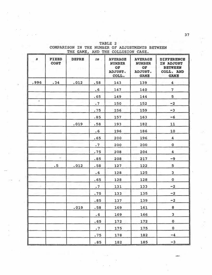
Table 2 expresses the. average number of adjustments obtained from

22 This dimension was absent in the former·· ~iterature, because they did not include fixed cost of adjustment.

.... c·

35

the sill\ulatio_ns23. , The , results,' furnish me 'with an idea of how the

frequency of capital adjustment varies between the game case and

the collusion case. This same measure was used in the analysis

above. In contl;"ast with the strategic complements case (Castal'\eda

'" .. (1992, (b»), the frequency of capital adjustment is higher under

the collusion solution than under the game solution for a degree of

interaction (DB) " equal to .58,.6, and .65. This is due to the

negative effect of the competitors's strategic variable (oapital)

on the firm's desired level of capital.

Any time the firm moves, it tries to further delay the move of the

other firm in such a way that it can maintain "Stackelberg"

leadership for that period of time. This performance by both

firms reduces the frequency of capital adjustments relatively to

the solution for the collusion case. Graphs one and four

illuminate this result . Note that the optimal response function

for the game solution is higher than the optimal response for the

collusion case. Secondly, due to the'''fact that depreciation is an

exponential process, depreciation tends to move the state towards

the area of partial preemption . As stated in the last section, ' the

policies of partial preemption have a strong effect in delaying the

adjustment of the rival for these degrees of interaction.

23 The procedure for calculating those numbers was stated in the last section. I followed an identiacal procedure for both the game- and the collusion case.

36

As we increase the fixed cost, we also see in Table 2 that, for a

degree of sUbstitution less than or equal to .65, the difference in

the average number of adjustments between the collusion case and

the game decreases. All else being equal, at higher levels of

fixed costs, the monopolists will try to economize. Hence, if .-'

fixed costs are large, the monopolist will reduce the number of

adjustments at a faster rate than the noncooperative duopolists do.

This phenom~na closes the gap in the frequency of capital

adjustments between the noncooperative duopolists and the

monopolist.

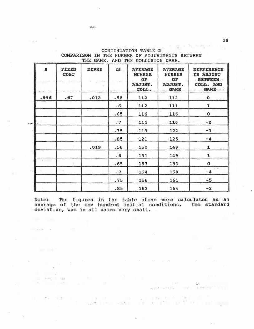
The results when (DB) equals. 7 , .75 and .85 are different. First,

we note that the frequency of capital adjustment is higher for the

game case than for the collusion case, although this difference is

small. By looking at graph one and two, we see that the area of

partial preemption is much smaller for low degrees of interaction

than for higher degrees. Furthermore, as noted above, the impact

of delaying the competitor's adjustment by preempting is much

smaller for low degrees of interaction than for larger degrees.

37

TABLE 2 COMPARISON IN THE NUMBER OF ADJUSTMEN'rS BETWEEN

THE GAME AND THE COLLUSION CASE . B FIXED DEPRB DB AVERAGE AVERAGE DIFFERENCE

COST NUMBER NUMBER IN ADJUST OF OF BETWEEN

ADJUST . ADJUST . COLL. AND COLL • GAME GAME

• 996 . 34 . 0l2 .58 143 139 4

.6 147 140 7

.65 149 144 5 . .7 150 152 -2

.75 156 159 -3

. 85 157 163 -6

. 019 .58 193 182 11

. 6 196 186 10

.65 200 196 4

. 7 200 200 0

.75 208 204 4

- . 85 208 217 -9

. 5 .0l2 .58 127 122 5

.6 128 125 3

.65 128 128 0

. 7 131 133 -2

.75 133 135 -2

.85 137 139 -2

.019 . 58 169 161 8

.6 169 166 3

.65 172 172 0

. 7 175 175 0

.75 178 182 -4

.85 182 185 -3

........

.. ~

38

CONTINUATION TABLE 2 COMPARISON IN THE NUMBER OF ADJUSTMENTS BETWEEN

'THE GAME AND THE COLLUSION CASE , . B FIXED DEPRE DB AVERAGE AVERAGE DIFFERQCB

COST NUMBER NUMBER IN ADJUST OF OF . BETWEEN · ..

ADJUST. ADJUST. COLL. AND , . " ', '. .COLL. '. GUE GUE .. ".'

.996 .67 .012 . 58 112 112 0 .. . . , . "

.6 112 111 1

.65 116 116 0

.7 116 118 -2

.75 119· 122 -3

.85 121 125 -4

.019 .58 150 149 1

.6 151 149 1

.65 153 153 0 . ..

. 7 154 158 -4

.75 156 161 ";5

.85 162 164 -2

Note: The figures in the table above were calculated as an average of the one hundred initial conditions. The standard deviation, was in all cases very small .

, .

39

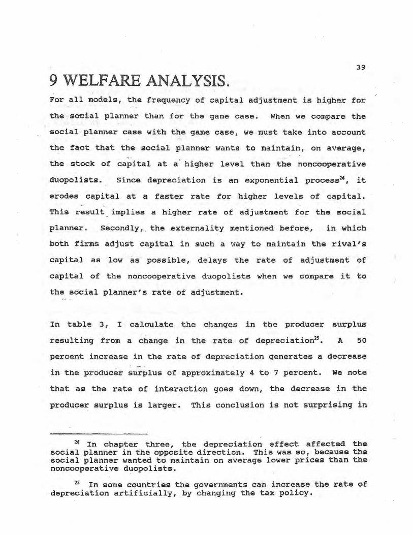
9 WELFARE ANALYSIS. For all models, the frequency of capital adjustment is higher for

the .social planner than for the game case. When we compare the

social planner case with the game case, we ·must take into account

the fact that the social p1anner wants to maintain, on average,

the stock of capital at a ' higher level than the noncooperative

duopolists. since depreciation is an exponential process24 , it

erodes capital at a faster rate for higher levels of capital. ..

This result .. implies a higher rate of adjustment for the social

planner . Secondly, the externality mentioned before, in which

both firms adjust capital in such a way to maintain the rival's

capital as low as possible, delays the rate of adjustment of

capital of the noncooperative duopolists when we compare it to

the social planner's rate of adjustment.

In table 3, I calculate the changes in the producer surplus

resulting from a change in the rate of depreciation25• A 50

percent increase in the rate of depreciation generates a decrease

in the producer surplus of approximately 4 to 7 percent . We note

that as the rate of interaction goes down, the decrease in the

producer surplus is larger. This conclusion is not surprising in

24 In chapter three, the depreciation effect affected the social planner in the opposite direction. This was so, because the social planner wanted to maintain on average lower prices than the noncooperative duopolists.

25 In some countries the governments can increase the r ate of depreciation artificially, by changing the tax policy.

40

view of the results found above. As the degree of interaction

decreases, the firms preempt less , and · ther efore increase the

frequency of investment. Consequently, we

industries that · are almost me>!lopolies (i. e.

conclude that in

those that exhibit

lower degrees of interaction), a higher rate of depreciation has

a greater impact on producer surplus than in more oligopolistic

industries.

" _. '.

41

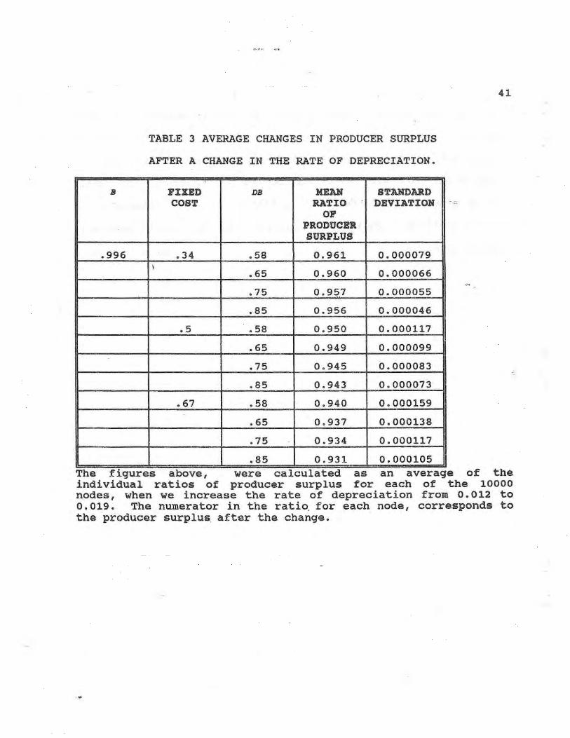
TABLE 3 AVERAGE CHANGES IN PRODUCER SURPLUS

AFTER A CH1L~GE IN THE RATE OF DEPRECIATION.

B FIXED DB MEAN STANDARD COST RATIO DEVIATION

OF PRODUCER SURPLUS

.996 .34 .58 0.961 0.000079 \

. 65 0.960 0.000066

. 75 0 . 957 0.000055

. 85 0 .956 0 . 000046

.5 .58 0.950 0.000117

.65 0.949 0.000099

.75 0 . 945 0.000083

. 85 0.943 0.000073

. 67 . 58 0.940 0 . 000159

.65 0.937 0.000138

. 75 0.934 0.000117

.85 0.931 0.000105 The f1gures above, were calculated as an average of the individual ratios Of producer surplus for each of the 10000 nodes, when we increase the rate of depreciation from 0.012 to 0.019. The numerator in the ratio. for each node, corresponds to the producer surplus after the change.

42

CONCLUDING REMARKS .

I have studyied a capital accumulation game, where fixed costs are

large enough to warrant inaction for some states for both firms,

but small enough to warrant the accommodation of both firms in the

market .

My results are reminiscent of the literature on preemption. One

firm will wait until the other firm is about to move. Then, in the

instant before the competitor is willing to move, the firm adjusts

its level of capital to the highest possible level achieved in the

game. This further delays the adjustment of the rival in its level

of capital. This behavior appeared consistently in all parameter

models considered in this work. However, the impact of these

policies appears to be larger for larger degrees of interaction.

The introduction of fixed adjustment costs provides a new dimension

in the analysis on quantity competition. In contrast with the

former literature on the subject, where Hanig (1986) and Maskin and

Tirole (1987), showed that, in equilibrium, symmetric firms will

maintain the same level of capital above the collusion level, my

research shows that, when we bring fixed adjustment costs into the

analysis, the firms will not keep the same level of capital 'all the

time. Rather, they will alternate in the level of of capital.

Furthermore, if we accept the assumption that firms choose prices

in such a way that they always produce at full capacity. This

43

model is a fully specified theory, that predicts alternations in

market share. " This prediction was necessarily absent in the

earlier literature.

When I compare the social planner's solution with the game's

solution, I conclude that the social planner ~djusts her variables

more frequently relative to oligopolistic firms . This result stems

from the fact that firms behave like "Stackelberg" leaders , and

consequently try to delay the adjustments of the competitor.

Secondly, since depreciation affects capital at an exponential

rate, and the social planner wants to maintain a higher level of

capital on average, depreciation further enhances the "Stackelberg"

effect .

with regard to the collusion case, I obtain mixed results. For a

high degree of interaction (DBs.6 5 ) , the two- product monopoly

(collusion) adjusts more frequently than the oligopolistic firms.

This result follows from the fact that both firms try to behave

like "Stackelberg" leaders , thereby delaying the adjustment in the

competitor's capital for as . long as they can. They do so by

adjusting right before the other firm wants to move . At the same

time , the fact that depreciation is an exponential process forces

the state to move towards the area of partial preemption ~ For

lower degrees of interaction (DB> . 65 ) , the collusive outcome adjust

less frequently than the oligopoly. For this case, the area of

partial preemption is much smaller, and its effect in terms of

44

delaying the adjustment of the rival is less important. The

Stackelberg effect is not strong enough to reverse the fact that

. the monopolist internalizes the costs of adjustment.

When we analyze the shape of the play set for the game case and the

monopoly case, we note :that the optimal response function for both

firms is higher for · the noncooperative duopolists than for the

collusive solution. Furthermore, the boundary betweeri the trigger

set for each firm and the continuation set, is located at a higher

level in the game solution than in the collusion case. All else

being equal, firms wait less time to adjust in noncooperative

environments than in the fully cooperative one.

'-" -'-.

Appendix 1. As mentioned in the main text the computational approach works in two stages. First I solve for the Nash equilibria in a square lattice with ~qually distant points in both dimensions so that T in equation (1) is exactly satisfied for any point in the lattice. Second, I look for an interpolation method that satisfies the piecewise differentiability imposed by the discretization of time. In this second procedure I choose a finite dimensional basis and represent our approximated value function in this subspace. Then through the iteration procedure I map this finite dimensional approximation into another finite dimensioanl approximation until I reach a level in which v·' is reasonably similar to v·'. As mentioned in the tex I use bilinear cardinal function because they span the space of purely continuous functions c' when the size of the grid tends to zero (the number of points go up to infinity), and therefore satisfies the property of piecewise differentiability of the theoretical value function. Secondly, this basis gives me computational speed. By definition of the bilinear cardinal functions, the coefficients which accompany this basis in the representation of the value function, equation (13) , are just the value function calculated in the solution of the Nash Equilibria at each node surrounding the point of interest for evaluating the function. In other words, the difficult task is to calculate the cardinal functions. Once these are calculated the projection coefficients (the 41 in (13» are trivially determined.

Given the properties of this model, it is not advisable to make use of the spectral methods that have been employed in economics to approximate the value function (See Judd 1990 (b». The use of Chebychev polynomials for example, imposes a degree of smoothness in the solution (C·) which is clearly undesirable for this problem. .

As mentioned already, the interpolation function is found by looking in ·the space of .bilinear functions for a function that best interpolates the value function in each of the squares. The next step is to patch together all of the small approximations and get a global approximation of the value function. The result will be a c· function.

More explicitly, follow.ing the technique of finite element, for each subsquare [x/ ,xt')X[x:,xt'], I use the information gotten from the first stage at each one of the nodes of this subsquare28

• I search for a bilinear function29 that best approximates the value function in this subsquare. In practice this is usually done by the use of the standard rectangle. The rectangle with vertices in the points (1,1), (-1,1), (-1,-1), (1,-1) • I map the value of x,.

28 In the context of this model, only the values of the operator TV',1

",

this information comprises at each of the nodes.

29 The class of bilinear functions is spanned by the monomials 1 , x , y . ,and ... xy •

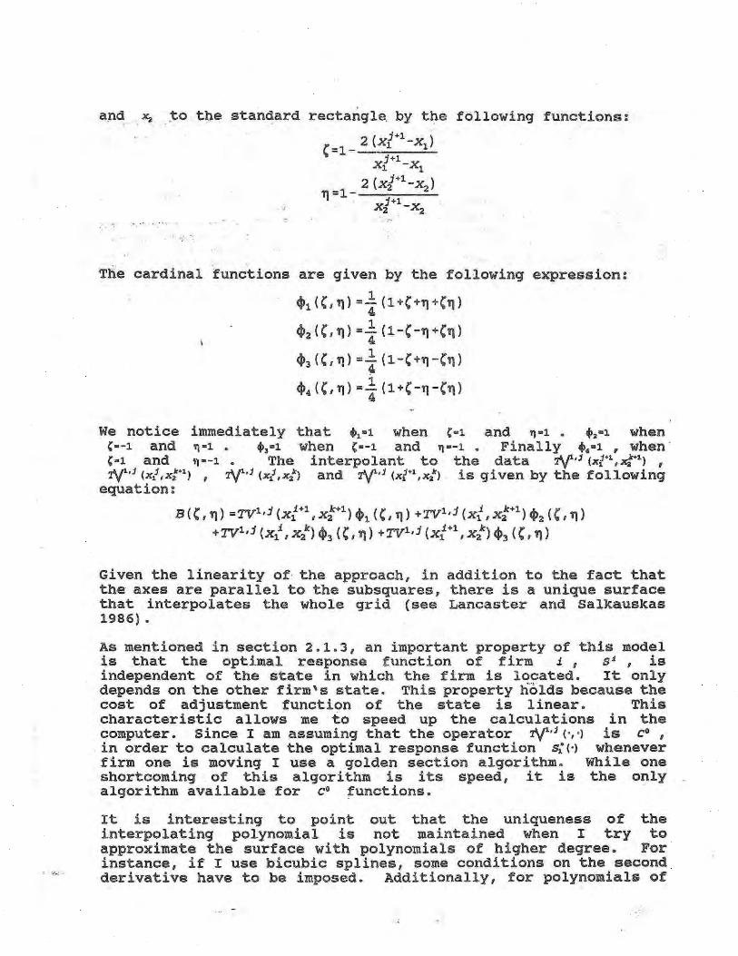
and. x. . . to the standard rectangle by the following functions:

( j+l .)

{=1 2 x, -x, xj+l_X

1 1

2(x j +l -x) 11 =1- 2 2

. j+l " X 2 . - X 2

, '-',

~ .'

The cardinal functions are given by the following expression:

~, ({,11) =10 (1+{+11+{11) 4

~2 ({,11) =! (1-{-11+'11)

~3 ({,11) =! (1-{+11-'11)

~4 ({,11) -! (1+{-11 -{11)

We notice immediately that 4>,-1 when ,-1 and ,,-1 . 4>,-1 when ,--1 and ,,-1. 4>,"1 when ,--1 and ,,--1 . Finally 4>,-1 , when ' ,-1 and ,,--1. The interpolant to the data '1'1/',1 (xt', xt') , '1'I/',j (xl,xt') , '1'I/',j (xl,x:) and '1'I/',j (xt',xJ) · is given by the following

equation :

B (C 11) _TV',j (xt' , xt') ~, (C 11) +TV',j (xt, X:+l) ~2 (C 11)

+TV',j (X,i , X2k) ~3 (C 11) +TV',j (xt' , xtl ~3 (C 11)

Given the linearity of the approach, in addition to the fact that the axes are parallel to the subsquares, there is a unique surface that interpolates the whole grid (see Lancaster and Salkauskas 1986) •

As mentioned in section 2.1.3, an important property of this model is that the optimal response function of firm i, 5', is independent of the state in which the firm is located. It only depends on the other firm's state. This property holds because the cost of adjustment function of the state is linear. This characteristic allows me to speed up the calculations in the computer. since I am assuming that the operator '1'I/',j (" .) is co,

. in order to calculate the optimal response function S;( . ) whenever firm one is moving I use a golden section algorithm . While one shortcoming of this algorithm is its speed, it is the only algorithm available for CO functions.

It is interesting to point out that the uniqueness of the interpolating polynomial is not maintained when I try to approximate the surface with polynomials of higher degree. For instance, if I use bicubic splines, some conditions on the second derivative have to be imposed. Additionally, for polynomials of

higher degrees, the cardinal functions do not . possess the small support property. In the linear case, the rational fOr using the cardinal functions is that they poss~ss the same nice properties as the B splines functions. In higher degrees, the Cardinal functions may not be easy to construct. The calculation may involve the inversion of a Vandermondian matrix, which we know is a dangerous procedure (see Lancaster and Salkauskas (1986». Consequently, if I want to extend the interpolation method to polynomials of second degree,- and hence allow for a higher degree of smoothness in the value function-, I should use B splines, since they maintain the. small support property and permit a more efficient the approximation.

. :-

. ; BIBLIOGRAPHY •.

Cl}rist.iano, L.J. (1990): "Solving the stochastic Growth Mod.::>l by Linear Quadratic Approximation and Value Function Iteration" Journal of Business and Economic Statistics, January 1990.

Qi.xit, A •. (1980): "The Role of Investment in Entry-Deterrence, '.' The . Economic Journal, 90, 95-106. . . ."

.,?uttal. P. and A. Rustichini (1990): "s-S Equilibria in stochastic . Games, .:with , im Application to Product Innovations;" mimeo. ,.Paper

t'resented in the S.I.T.E. semiriar at Stanford University summer 1991.

Eaton, B.C. and R.G. Lipsey (1980): Barriers, the Durability of Capital as Journal of Economics, 12, 593-604.

"Exit Barriers and Entry a Barriez: .• to Entry," Bell

Fudenberg, D. and J. Tirole (1983): "Capital as Commitment: Strategic Investment to Deter Mobility," Journal of Economic Theory, 31, 227-250 .

Fudenberg, D. and J. Tirole (1991): Game Theory. Cambridge: MIT Press.

Hanig, M. (1986): Differential Gaming Models of Oligopoly. Ph.D. thesis, Department of Economics, Massachusetts Institute of Technology.

Hansen, L.P. and T.J. Sargent (1990) : "Recursive Linear Models of Dynamic Economics,'" mimeo, Hoover Institution.

Judd, K. (1985): "Closed Loop Equilibrium Innovation Race," Discussion Paper 647, Kellog Management, Northwestern University .

in a Multi-Stage Graduate School of

Jl.!dd, K. (1990(a»: "Cournot vs. Bertrand : A Dynamic Resolution," mimeo, Hoover Institution.

Judd, K. (1990(b»: "Minimum Weighted Residual Models for Solving Dynamic Economic Models," mimeo, Hoover Institution. .

....... Lancaster, P. and K. Salkauskas (1986): Curve and Surface Fitting. San Diego: Academic Press.

Maskin E. and J. Tirole (1987): "A Theory of Dynamic OlI'gopoly, . III: Cournot Competition," European Economic Review, 31, 947-968.

Maskin E. and J. Tirole (1988 (b»: "A Theory of Dynamic Oligopoly, I: Overview and Quantity Competition with Large Fixed costs," Econometrica, 56, ??-570 • .

Spence, A.M. (1977): "Entry, capacity, Investment and Oligopolistic Pricing," Bell Journal of Economics, 8, 534-544.

sulem, A. (1986) : "Explicit Solution of a Two Deterministic Inventory Problem," Mathematics of Research, 11, 134-146.

Dimensional Operations

Tirole, J. (1988): The Theory of Industrial Organization. Cambridge: MIT Press.

Villas-Boas, J.M. · " 'C1990): "Dynamic Duopolies with Non-Convex Adjustment costs," mimeo, Massachusetts Institute of Technology.y

SERlE DOCUMENTOS DE TRABAJO

The following working papers from rece.nt years are st i ll available upon request from :

Rocio contreras, Centro de Documentaci6n, ' Centro De Estudios Econ6micos,. EI Colegio de Mexico A.C . , Camino al Ajusco # 20 C. P. 01000 Mexico, D. F .

90/1

90/II

I~e, Alain . "Trade liberalization , stabilization , and growth: some notes on the mexican experience".

Sandoval Musi , Alfredo . "Construction of new monetary aggregates: the case of Mexico".

90/rI:i" " Fernandez, Oscar . "Algunas notas sobre los modelos de Kalecki del ciclo econ6mico" .

90/IV

90/V

90/VI

Sobarzo " Horacio E. "A 'consolidatedsocial accounting matri x for input- output analysis" .

' .. ".urzua, Carlos M. "El deficit del sector publico y. . . la poiitica fiscal en Mexico, . 1980 . - 1989" •.

Romero, Jose . "Desarrollos recientes en la teoria econ6mica de la uni6n aduanera".

90/VII Garcia Rocha, ,Adalberto. "Note on mexican economic deve).opmeqt ,and. income distribution" .

90/VIII Garcia Rocha, Adalberto . " Distributive effects of ·:final!~iCll jpolie:ies in Mexic,o".

90/IX Mercado , Alfonso and Taeko Taniura "The mexican automotive export growth : favorable factors , obstacles and policy requirements" .

91/1 Urzua , Carlos M. "Resuelve : a Gauss program to solve applied equilibrium and disequilibrium models" .

91/11 Sobar zo, Horacio E. "A general equilibrium analysis of the gains from trade for t he mexican economy of a North American free t r ade agreement" .

9l/III

9l/IV

9l/V

9l/VI

92/I

92/II

92/III

92/IV

92/V

92/VI

93/I

93/II

93/III

Young, Leslie and Jose Romero . "A dynamic dual model of the North American free trade agreement".

Yunez - Naude, Antonio. "Hacia un tratado de libre comercio norteamericano; efectos en los sectores agropecuarios y alimenticios de Mexico" .

Esquivel, Hernandez Gerardo. "Comercio intraindustrial Mexico-Estados Unidos".

Marquez, Colin Graciela. "Concentraci6n y estrategias de crecimiento industrial" .

Twomey, J. Michael. "Macroeconomic effects of trade liberalization in Canada and Mexico".

Twomey, J . Michael. "Multinational corporations in North America: Free trade intersections".

Izaguirre Navarro, Felipe AC

• "Un estudio empirico sobresolvencia del sector publico: El caso de Mexico".

Gollas, Manuel y Oscar Fernandez. "El subempleo sectorial en Mexico".

Calder6n Madrid, Angel. "The dynamics of real exchange rate and financial assets of privately financed current account deficits"

Esquivel Hernandez, Gerardo. "Politica comercial bajo competencia imperfecta: Ejercicio de simulaci6n para la industria cervecera mexicana".

Fernandez, Jorge. "Debt and incentives in a dynamic context" .

Fernandez, Jorge. "Voluntary debt reduction under . asymmetric information".

Castaneda, Alejandro. "Capital accumulation games".