DOCUMENTOS DE TRABAJO

Taxonomy of Chilean Financial Fragility Periods from 1975 to 2017

Juan Francisco MartínezJosé Miguel MatusDaniel Oda

N° 822 Junio 2018BANCO CENTRAL DE CHILE

BANCO CENTRAL DE CHILE

CENTRAL BANK OF CHILE

La serie Documentos de Trabajo es una publicación del Banco Central de Chile que divulga los trabajos de investigación económica realizados por profesionales de esta institución o encargados por ella a terceros. El objetivo de la serie es aportar al debate temas relevantes y presentar nuevos enfoques en el análisis de los mismos. La difusión de los Documentos de Trabajo sólo intenta facilitar el intercambio de ideas y dar a conocer investigaciones, con carácter preliminar, para su discusión y comentarios.

La publicación de los Documentos de Trabajo no está sujeta a la aprobación previa de los miembros del Consejo del Banco Central de Chile. Tanto el contenido de los Documentos de Trabajo como también los análisis y conclusiones que de ellos se deriven, son de exclusiva responsabilidad de su o sus autores y no reflejan necesariamente la opinión del Banco Central de Chile o de sus Consejeros.

The Working Papers series of the Central Bank of Chile disseminates economic research conducted by Central Bank staff or third parties under the sponsorship of the Bank. The purpose of the series is to contribute to the discussion of relevant issues and develop new analytical or empirical approaches in their analyses. The only aim of the Working Papers is to disseminate preliminary research for its discussion and comments.

Publication of Working Papers is not subject to previous approval by the members of the Board of the Central Bank. The views and conclusions presented in the papers are exclusively those of the author(s) and do not necessarily reflect the position of the Central Bank of Chile or of the Board members.

Documentos de Trabajo del Banco Central de ChileWorking Papers of the Central Bank of Chile

Agustinas 1180, Santiago, ChileTeléfono: (56-2) 3882475; Fax: (56-2) 3882231

Documento de Trabajo

N° 822

Working Paper

N° 822

Taxonomy of Chilean financial fragility periods from

1975 to 2017

Juan Francisco Martínez

Banco Central de Chile

José Miguel Matus

Banco Central de Chile

Daniel Oda

Banco Central de Chile

Abstract

The measurement of financial fragility is a key element but still an ongoing task for monetary,

financial authorities and international financial institutions. This is specially relevant when applying

financial policies that are contingent on the behavior of a particular economy or try to anticipate

disruptive events. However, there are several dimensions that complicate the precise definition of

financial fragility and the identification of these periods; some examples are: the distinction of causes,

symptoms, effects and policy management measures. The current literature points out to a few key

elements that have a broad impact on the financial system. In particular, it highlights the role of

materialized credit risk, profits and credit activity of banks as signs of instability. In this paper, we

combine these elements to identify and delimit historical financial fragility periods for the Chilean

economy. In doing so, we build a novel monthly database that includes the 1980's local banking crisis

period.

Resumen

La medición de la fragilidad financiera es un elemento clave, pero sigue siendo un desafío para las

autoridades monetarias, financieras y las instituciones financieras internacionales. Esto es

especialmente relevante cuando se aplican políticas financieras que dependen del comportamiento de

una economía en particular o cuando se intenta anticipar eventos disruptivos.

Sin embargo, hay varias dimensiones que complican la definición precisa de fragilidad financiera y la

identificación de estos períodos; algunos ejemplos son: la distinción de las causas, síntomas, efectos y

medidas de gestión de crisis. La literatura actual señala algunos elementos clave que tienen un amplio

impacto en el sistema financiero. En particular, se destaca el papel del riesgo de crédito materializado,

la rentabilidad y la actividad crediticia de los bancos en la detección de inestabilidad financiera. En

este documento, se combinan dichos elementos para identificar y delimitar los períodos históricos de

fragilidad financiera para la economía chilena. En el proceso, se recopila información y se genera una

base de datos que incluye el período de crisis bancaria local de los años ochenta.

We are grateful to Karina Araya and Pablo Carvajal for their excellent research assistance. Special thanks to Rodrigo Alfaro,

Solange Berstein, Christian Castro, Rodrigo Cifuentes, Andrew Powell, and Claudio Radatz, for their comments and suggestions

at different stages of this work. The opinions expressed in this article are the authors' own and do not necessarily represent the

views of the Central Bank of Chile or its Board Members.

Emails jmartinez@bcentral.cl, jmatus@bcentral.cl, dodaze@bcentral.cl.

1 Introduction

Monetary policy development and implementation has been favored by a def-inition of price stability, measured through in�ation. The use of a single indi-cator simpli�es the decision making process for most monetary authorities andcontributes to its accountability (Goodhart, 1989). However, the application of�nancial policies has been less precise and established since there is no full con-sensus about the object of analysis: the �nancial fragility (Goodhart, 1989, Borio& Drehmann 2009).

Financial fragility concept has been widely studied, especially after the recentglobal �nancial crisis. On the one hand, prudential monitoring has been incorpo-rating a wide range of �nancial indicators that help in the aggregate judgementof the �nancial situation of an economy. That is how several Financial StabilityReports - of developed and developing countries �nancial authorities' (Lim et al.,2017) - have emerged and progressed in coverage and technical depth of the anal-ysis of aggregate risks that potentially a�ect the system. Although the �nancialmonitoring constitutes a valuable input to ensure the stability of the �nancialsystem, the implementation of macro-prudential policies has not been straightfor-ward because of the lack of a unique indicator, as in the case of monetary policy,among other di�culties (Goodhart, 1989). In this context, it is often necessary touse several metrics to de�ne historic periods of �nancial fragility to systematicallyanalyze this �nancial phenomenon, and thus, collect lessons that allow a correctimplementation of �nancial policies.

The design of policies that are focused on anticipate, prevent and mitigate thee�ects of �nancial fragility periods, requires a precise de�nition of its previousoccurrences. For example, in the design of the Counter-Cyclical Capital Bu�er,it is necessary to test the properties of several indicators in their ability to antici-pate periods of �nancial fragility that are originated by an excessive credit growth(Borio, 2014). By assuming that there is an historical regularity, it is reasonableto undertake a retrospective analysis that attempts to measure the predictivepower of early warning indicators on past fragility episodes, such as the AUROC1. However, although it is di�cult to �nd clear evidence in the related literature(e.g. Detken et al (2014)), a delimitation of �nancial fragility periods has to beperformed before the analysis of the early warning indicators.

There is no formal de�nition nor a consensus about �nancial fragility - or �-

1De�ned as the Area Under the Operator Characteristics Curve. For details, see Detken et al.(2014).

2

nancial stability - measures (Borio & Drehmann, 2009, Goodhart, 1989). Somemetrics are based on historical events of excessive assets volatility (e.g. Merton,1974), high probabilities of default and low pro�tability of banks (Goodhart et al.,2006), or - in the case of banking crises - bankruptcies of �nancial institutions andseveral dimensions of imbalances or risk (Leaven & Valencia, 2008). Although theymay di�er in their nature and methodology, all of these approaches aim to capturea systemic component of risks. That is, a period of fragility should be charac-terized by a small set of factors or variables that re�ect the systemic vulnerability.

In particular, there is some evidence in the identi�cation of fragility periodsin the Chilean economy, but it is still necessary to work on the precision andhistorical depth of the delimitation of particular periods. The Chilean economyhas experienced various episodes of �nancial turmoil, where the crisis of the 80'sis clearly distinguished by its magnitude and the relevance of government inter-ventions. In fact, it is considered as one of the episodes that had the largest �scalimpact above a wide set of economies (Laeven & Valencia, 2012).

Regarding the period nearby the so-called Asian Crisis (1998-1999) and theGlobal Financial Crisis (2008-2009), there are few studies that investigate some�nancial stylized facts in the Chilean economy. Since the 90's Chile has experi-enced a stable period with practically nonexistent disruptions. In this context,Ahumada & Budnevich (2002) investigate the properties of a set of �nancial vari-ables as early warning indicators of �nancial fragility in Chile. In their estimations,they assume that past due loans and inter-bank spreads re�ect �nancial fragility.On the other hand, De Gregorio (2009), points out that around to the GlobalFinancial Crisis a liquidity shock of international �nancial markets a�ected theChilean economy with some real consequences. Nonetheless, the e�ects of theshock were limited by the solid macroeconomic and �nancial environment, andthe policy measures taken.

Despite the progress of the current literature, it is still necessary to providea more complete and precise identi�cation of �nancial fragility periods. First,we need a set of variables that allows us to identify contemporaneous �nancialfragility in a context where, as it has been emphasized, the de�nition of the con-cept is di�use and encompasses many dimensions. Therefore, we have to presenta speci�c �nancial fragility taxonomy. Second, we have to consider that more re-cent episodes had a considerably lower �nancial and macroeconomic impact. And�nally, recognize that there is a lack of �nancial data in terms of homogeneity ofde�nitions, time coverage and frequency. Thus, this paper addresses these issuesand suggest precise dates for the beginning and end of �nancial fragility episodesin Chile, on a monthly basis, since 1975.

3

The remaining part of this paper is organized as follows. Section 2 providesa conceptual framework of �nancial fragility taxonomy. Section 3 presents thecriteria in the elaboration of a �nancial database for the Chilean economy. Section4 shows the empirical methodology, analysis and delimitation of �nancial fragilityperiods. Section 5 complements the statistical analysis with an historical contextthat illustrate the interaction of macro and �nancial elements in the fragilityepisodes. Finally, section 6 concludes.

2 Towards a �nancial fragility taxonomy

In order to perform the empirical analysis, we de�ne the main dimensions of�nancial fragility that are in our focus. Thus, we develop a taxonomy that consistson discriminating among di�erent dimensions and events around fragility periods.Consequently, we look for an operational de�nition of the concept that allows usto take the theory to the data.

Various authors have pointed out the necessity and di�culties to discern �-nancial fragility periods owing to the fact that this concept overlaps with others,such as economic fragility, and economic and banking crisis (Allen & Gale, 2004;Goodhart et al., 2006; Claessens & Kose, 2013). Generally, by looking at �nancialand economic data for a broad set of economies, it can be argued that not all�nancial fragility periods are preceded or followed by an economic downturn. Forexample, the �dot com bubble burst" in 20002 was relatively well isolated fromthe real and �nancial sectors, especially because it was not �nanced with debt butequity (Brunnermeier & Schnabel, 2016).

Additionally, not all �nancial fragility periods involve banks. However, whenbanks are a�ected, the impacts on the macro-economy are more sizeable (Rein-hart & Rogo�, 2009). Furthermore, not all periods of fragility end up in crises.Thus, the analysis has to be especially cautious to distinguish the key elementsof �nancial fragility. In that sense, our study is focused on the involvement of thebanking system, but also considers the economic context distinguishing betweeni) causes, ii) characteristics or symptoms, and iii) e�ects and policy measures.Additionally, we describe historical circumstances and the changes in the reg-ulatory framework. As previously noted, the de�nition of �nancial stability isstill subject of debate in academic and macro �nancial policy forums (Borio &Drehmann, 2009). This discussion highlights the need and di�culty of identifyingperiods of �nancial fragility (Allen & Gale, 2004; Goodhart et al., 2006; Claessens& Kose, 2013), since there is a signi�cant overlap with other concepts. However,

4

several advances have been made in the distinction of its fundamental elements.In this work, we rely on this progress to characterize the dimensions that re�ectthe strength or vulnerability of the banking sector. In other hand, we know thatMinsky (1972) describes people that have misalignment in expectations througha form of myopia around good states of nature or booms. This generates excessrisk taking and could propitiate �nancial fragility.

Favorable conditions for a �nancial fragility occurrence: causes

and consequences

Although to de�ne the causality between macroeconomic and �nancial fragilityis a challenge, there are some economic and �nancial factors that may propitiatethe occurrence of a �nancial fragility period or, in extreme cases, a crisis. Allen& Gale (2004) indicates that a �nancial system is unstable or fragile when thereare conditions under which small shocks may cause major disruptions. In theeconomic literature there are di�erent emphasis on the role of the �nancial sector.

For instance, Reinhart & Rogo� (2009) suggests that the traditional �nancialcrisis concept refers to events that were not originated in the real sector. How-ever, it is indirectly associated with �nancial or monetary systems imbalances thatmay cause considerable �uctuations in asset prices, that a�ect the �nancial insti-tutions capacity to ful�ll their obligations. On the other hand, macroeconomicfactors such as policies or expectations that may a�ect the quality of bank assets,its funding costs, liquidity and credit dynamics, may induce �nancial fragility pe-riods. Hausmann & Rojas-Suárez (1997) includes factors such as the excessiveexpansion of monetary aggregates, the e�ect of public expectations and, internaland external volatilities. Some external factors are the excessive capital in�ows(Reinhart & Rogo�, 2009; Laeven & Valencia, 2008), current account and �scalde�cits (Laeven & Valencia, 2008), anomalous asset price �uctuations (Reinhart& Rogo�, 2009 and Claessens et al., 2013).

In reference to microeconomic causes, these are often related to i) weaknessesin banking regulation and supervision (Claessens et al., 2013 and Laeven & Valen-cia 2008), ii) disorganized �nancial liberalization schemes (Claessens et al., 2013,and Laeven & Valencia 2008), iii) inadequate accounting frameworks, (Laeven &Valencia, 2008), iv) excessive banking credit growth (Borio, 2014; Claessens etal., 2013; Reinhart & Rogo�, 2009; Laeven & Valencia, 2008 and Minsky, 1972),v) (excessively) �exible loan terms (Claessens et al., 2013) and vi) high leverage(Minsky (1972), among others.

Finally, regarding to the consequences of �nancial fragility, in extreme cases,

5

such as banking crises, the need for governmental intervention arises to reduce thenegative e�ects (Claessens et al., 2013). Thus, as Leaven & Valencia (2008, 2012)propose, a banking crisis may cause an important detriment of government �scalstance. Alternatively, Demirgüç-Kunt & Detragiache (1997) indicate that bankingfragility periods are followed by bank nationalization. In a less extreme situationof �nancial fragility, De Gregorio (2009) suggests that the policy interventioninvolves liquidity easing to vulnerable sectors.

Banking crises and �nancial fragility identi�cation

Banking crises are extreme events of �nancial fragility periods and have mul-tiple causes and e�ects, and several dimensions. Nonetheless, we will focus onthese types of events and also on milder �nancial fragility periods that are asso-ciated with the banking sector. The approach followed is based on the selectionof banking (Shin, 2013) and coincident2 (Logan, 2001) ratios. Although the ele-ments of banking crises and �nancial fragility are present in the literature for along time, they are often confused and mixed. For instance, Laeven & Valencia(2008, 2012) indicate that banking crisis periods can coincide with those of debtand currency. But, it has to be emphasized that there is no full overlap amongthese events. Moreover, when it comes to characterize banking crises periods, theauthors include i) excessive losses because of rising non-performing loans and ii)signi�cant �scal costs of government intervention.

The selection of key variables

With the considerations of previous sections, we focus on variables that ac-count for the symptoms rather than causes and consequences of disruptive eventsof �nancial fragility.

Table 1 is an extension of Amieva & Urriza (2000) which summarizes the setof relevant characteristics used in the literature. Among the symptoms that thebanking sector experiences we highlight: (i) the increase in the delinquency rate(ii) insolvencies of banking institutions, (iii) liquidity constraints, (v) credit re-strictions and (vi) balance-sheet e�ects. This evidence covers �nancial fragilityperiods as well as banking crises.

2An indicator that moves simultaneously with the �nancial environment and therefore re�ects itscurrent status.

6

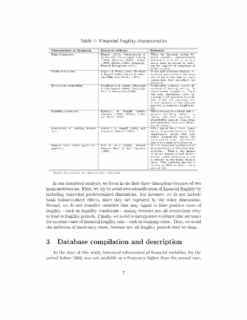
Table 1: Financial fragility characteristics

Characteristic or Symptom Research evidence Rationale

High delinquency Minsky (1972), Sundararaján &Baliño 1991, Guttentag & Herring(1984), Manikow (1986), Veblen(1904), Mitchell (1941), Demirgüç-Kunt & Detragiache (1997).

When the �nancial system be-comes unstable, macroeconomic(internal or external) or liquidityshocks have an impact in reduc-ing the capacity of repayment ofbanks' debtors.

Credit restrictions Stiglitz & Weiss (1981), Reinhart& Rogo� (2009), Laeven & Valen-cia (2008) and Minsky (1972).

Severe and persistent liquidity re-strictions and excessive risk aver-sion of banks may lead to creditcontractions that exacerbate thedownturn.

Decrease in pro�tability Goodhart et al. (2006), Albertazzi& Gambacorta (2009), Demirgüç-Kunt & Detragiache (1999).

Pro�tability contains several di-mensions of banking activity. Itmixes market competition, �nan-cial costs, operational costs, in-creasing in delinquencies material-ized in loan loss provisions, etc.A high variation of this indicatormay well account for a fragility pe-riod.

Liquidity constraints Reinhart & Rogo� (2009),Schwartz (1985), Wolfson (1986)and Mirön (1986)

When solvency is a threat and re-payment are being reduced, in-vestors hold their resources toavoid further impacts. Thus, �rmsand banks face short term �nanc-ing restrictions.

Insolvencies of banking institu-tions

Reinhart & Rogo� (2009) andLaeven & Valencia (2008).

When agents lower their repay-ments, in general, there are othersimultaneous shocks that mayreduce dramatically banks' networth and solvency. An extremecase of this leads to insolvencies.

Balance sheet e�ects (price andquantity)

Bell & Pain (2000), FederalReserve Bank of San Francisco(1985).

This is somewhat predeterminedby a combination of the other char-acteristics. That is, the impacton bank's depositors and debtorsand the market valuation of a bankis re�ected in the banks' balancesheet. This condition also has areinforcing e�ect on other dimen-sions of risk.

Source: Own elaboration based on listed references.

In our statistical analysis, we focus in the �rst three dimensions because of twomain motivations. First, we try to avoid over-identi�cation of �nancial fragility byincluding somewhat predetermined dimensions. For instance, we do not includebank balances-sheet e�ects, since they are captured by the other dimensions.Second, we do not consider variables that may signal to false positive cases offragility - such as liquidity conditions -, mainly because not all restrictions obeyor lead to fragility periods. Finally, we avoid to incorporate evidence that accountsfor extreme cases of �nancial fragility only - such as banking crises. Thus, we avoidthe inclusion of insolvency cases, because not all fragility periods lead to them.

3 Database compilation and description

At the date of this study, historical information of �nancial variables, for theperiod before 1989, was not available at a frequency higher than the annual rate,

7

which made it di�cult to characterize the �nancial sector. For this reason, in thiswork, we compile a new database that allows us to estimate metrics of �nancialfragility and incorporate the dynamics of key variables suggested by the literature.

This section describes the criteria used to construct the database of �nancialbanking variables. This is used afterwards in the the de�nition of �nancial fragility(i.e. past-due loans ratio, pro�tability and banking credit growth/contractions)and in the characterization or context of those periods (i.e. other macroeconomicand �nancial variables). The speci�c details on variables construction and sourcesis available in Appendix 2.

3.1 Banking data

From January 1970 to December 1988, the information of the printed bul-letins of the Superintendency of Banks and Financial Institutions (SBIF) wasused. Since January 1989, the information on the main �nancial statements ofthe banks (balance sheets and income statements) are digitized.

In general, the criterion for constructing the database of the banking systemwas to maintain current standards in order to make comparable di�erent seriesof banks since 1970. Over the last decades, the accounting format of banks hadsigni�cant changes. Two of the most important occurred in August 1985, with alocally originated modi�cation introducing new balance-sheet and income state-ments models, and in January 2008, with the introduction of the InternationalFinancial Reporting Standards (IFRS).

Between 1975 and 1978, "Financial Companies" information was available.This group includes several �nancial �rms - formal and informal - that were devel-oped under the "free banking" framework. After three years, these were dissolvedor absorbed by other �nancial institutions. These companies grew explosively dueto the lack of an appropriate regulatory framework. Therefore, the informationof this group was excluded in the elaboration of the series, because they distortedthe dynamics of the �nancial system we want to capture.

The printed bulletins of the SBIF between 1970 and 1978 are available in thelibrary of the Superintendency and only from 1979 are available in the library ofthe CBC. This information was homologated as is detailed in Appendix 2.

8

3.2 Macroeconomic data

The main source of information is the Statistical Database from the CentralBank of Chile (CBC). This dataset contains copper price series, unemploymentrates, GDP, current account de�cit and exchange rate. Additionally, from theChilean Copper Commission (COCHILCO) we obtain monthly data of copperpound price (nominal and constant) from 1960.

The unemployment rate is available from 1970 and was extracted from theCentral Bank of Chile (2001). These data are merged with quarterly data alsopublished in the CBC statistical database named "Quarterly Unemployment Ratein Greater Santiago." The reason for extracting the unemployment rate from theGreater Santiago is due to its time coverage and the similarity with the unemploy-ment data at national level published by the Instituto Nacional de Estadísticas(INE).

The current account de�cit was obtained from the statistical database "His-torical Information of Balance of payments of External Sector" of the CentralBank of Chile . Because the quarterly information is only available since 1996, itwas considered an annual frequency to privilege the most historical information,dating from 1960.

For the exchange rate, we used the CBC statistical database named "Histor-ical Information of Exchange Rates of Observed Dollar". In addition, the realexchange rate index was obtained from the same information source, but onlyfrom the �rst quarter of 1986.

Finally, the Consumer Price Index (CPI) was also obtained from the statisticaldatabase of the CBC "Historical Information of Annual Variation of Prices".

4 Empirical Analysis: methodology and results

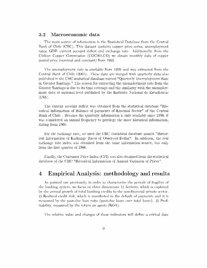
As pointed out previously, in order to characterize the periods of fragility ofthe banking system, we focus on three dimensions 1) Activity, which is capturedby the annual growth of total banking credits to the non-�nancial private sector.2) Realized credit risk, which is manifested in the default of payments and it ismeasured by the past-due loan ratio (past-due loans over total loans). 3) Prof-itability, measured by the return on assets (ROA).

The relative value and changes of these indicators will de�ne a critical date

9

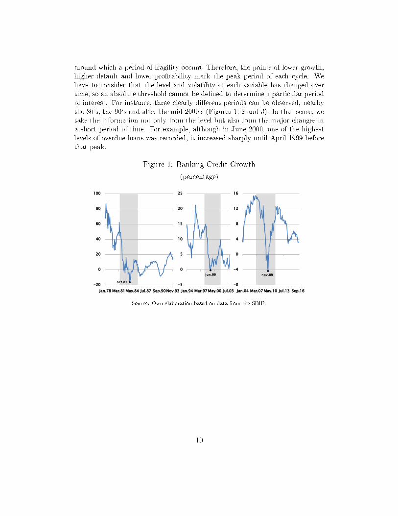
around which a period of fragility occurs. Therefore, the points of lower growth,higher default and lower pro�tability mark the peak period of each cycle. Wehave to consider that the level and volatility of each variable has changed overtime, so an absolute threshold cannot be de�ned to determine a particular periodof interest. For instance, three clearly di�erent periods can be observed, nearbythe 80's, the 90's and after the mid 2000's (Figures 1, 2 and 3). In that sense, wetake the information not only from the level but also from the major changes ina short period of time. For example, although in June 2000, one of the highestlevels of overdue loans was recorded, it increased sharply until April 1999 beforethat peak.

Figure 1: Banking Credit Growth

(percentage)

-5

0

5

10

15

20

25

Jan.94 Mar.97May.00 Jul.03

-8

-4

0

4

8

12

16

Jan.04 Mar.07May.10 Jul.13 Sep.16

-20

0

20

40

60

80

100

Jan.78 Mar.81May.84 Jul.87 Sep.90Nov.93

oct.83

jun.99 nov.09

Source: Own elaboration based on data from the SBIF.

10

Figure 2: Past-due Index

(percentage of total loans)

0

3

6

9

12

15

Jan.78 Mar.81May.84 Jul.87 Sep.90Nov.93

0,0

0,5

1,0

1,5

2,0

2,5

Jan.94 Mar.97May.00 Jul.03

0,0

0,4

0,8

1,2

1,6

2,0

Jan.04 Mar.07May.10 Jul.13 Sep.16

jul.83

apr.99

jun.09

jul.10

jun.00

Source: Own elaboration based on data from the SBIF.

Figure 3: Return on Assets (ROA)

(percentage)

0,5

0,7

0,9

1,1

1,3

1,5

1,7

Jan.04 Mar.07May.10 Jul.13 Sep.16

-3

-2

-1

0

1

2

3

Jan.78 Mar.81May.84 Jul.87 Sep.90Nov.93

0,0

0,5

1,0

1,5

2,0

2,5

3,0

Jan.94 Mar.97May.00 Jul.03

oct.08

oct.99jul.83

jan.85

Source: Own elaboration based on data from the SBIF.

11

4.1 Empirical strategy

We can summarize the mechanism to de�ne fragility periods into two steps.First, we propose a coincident indicator of �nancial fragility. Using this indicatorwe mark critical dates or candidates for fragility episodes at the lowest peak of acombination of �nancial variables. Second, by looking at the slope of the index,we delimit the beginning and the end of each period around the selected dates.

Financial Fragility metrics

Business cycles and �nancial stability metrics available in the literature at-tempt to summarize the behavior of a set of variables to identify periods wherethis set reports some relevant misalignment.

In order to forecast the GDP cycle, Stock & Watson (1999) reduced 215 vari-ables into few indicators or factors using factor analysis. The factor analysiscalculates linear combinations (factors) of a number of variables that maximizesthe variance of the factor. In the same way, the Federal Reserve Bank of Chicagoused 85 indicator to construct the Chicago Fed National Activity Index (CFNAI)based on this framework3.

Alternatively, Eichengreen et al. (1996), for example, used models such asprobit and logit to estimate the probability of the fragility periods based on a setof variables. However, it requires necessarily an ex-ante de�nition of the episodes.Since we do not have pre-de�ned periods, this method is unviable.

Another approach is to combine key variables using a transformation basedon their observed cumulative distribution functions (CDF). Using this method,the variables are transformed to percentiles and then averaged. Additionally, anindex of fragility can be calculated by counting the number of indicators above athreshold, such Edison (2003), Goldstein et.al (2000), and Kaminsky (1999).

Likewise, the variance-equal weights method use a simple average of the stan-dardized variables assuming a normal distribution. The IMF constructs the Fi-nancial Stress Index (FSI) as the variance-weighted average of three subindicesassociated with the banking, securities, and foreign exchange markets, based onIlling and Liu (2006)4. Bordo et al. (2002) used a version of a standardized

3For further details, see Federal Reserve Bank of Chicago (2016).4They calculate a Financial Stress Index for Canadian �nancial system and concludes that the

standard-variable version has the lowest Types I and II errors compared with other measures commonlyused in the literature.

12

distance from the median in order to avoid the skewness of the series and alsoseparate the analysis in two di�erent sub periods.

Typically, the objective of constructing a �nancial index is to foresee periodsof distress. In this sense, the associated methodologies are adjusted in order tocapture past crises. Therefore, its usefulness is related to its predictive power.Likewise, using these tools to de�ne periods of �nancial fragility could have prob-lems of endogeneity5 and temporality6. In this context, instead of anticipating�nancial fragility periods this paper seeks to generate an index that determinesperiods of historical �nancial distress in order to characterize them.

Peaks of �nancial fragility

As previously explained, the �rst estimation step consists of summarizing theset of coincident �nancial indicators into one index. As we described in the pre-vious sections, the �nancial variables has di�erent levels between them and overtime. A common technique to scale a variable is standardized it by subtractingits mean and divided it by its standard deviation. The standardized value can beinterpreted as the deviation of the variable from its expected value (approximatedby its mean). Since the characterization of fragility periods is an ex-post analysis,we observe the realization of the variable around a particular point in time. Thus,a value in the tail of the distribution is considered as critical.

An advantage of the standardization is that we are able to compare variablesthat were initially in di�erent scales. Consequently, we can calculate linear com-binations of each characteristic without being a�ected by the original units northe changes in levels and volatilities over time.

With respect to the linear combinations, we have to de�ne the weights of eachdimension. One option is use weights obtained by the factor analysis approach.These weights are �xed in time and depends on the sample period. However, fac-tor analysis is more useful when working with a high number of variables, whichis not our case. On the other hand, the use of the historical distribution requiresan enough large sample window to provide seemingly continuous distributions,and since we are using the values at the tails, the index is a�ected by extremevalues. Therefore, we use the variance-equal weights method, which is simple andhave a very straight forward interpretation. Additionally, as Bordo et al. (2002),we extend its calculation for a several time windows, although we use the normal

5The de�nition of crisis is based on the same metric which tries to predict it.6We can only observe the state of nature after it was resolved. For example, the minimum value

of a variable in a period.

13

distribution7.

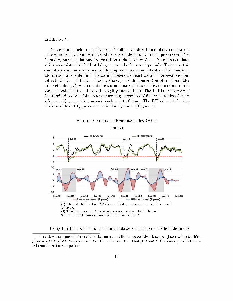
As we stated before, the (centered) rolling window frame allow us to avoidchanges in the level and variance of each variable in order to compare them. Fur-thermore, our calculations are based on a data centered on the reference date,which is consistent with identifying ex-post the distressed periods. Typically, thiskind of approaches are focused on �nding early warning indicators that uses onlyinformation available until the date of reference (past data) or projections, butnot actual future data. Considering the exposed di�erences (set of used variablesand methodology), we denominate the summary of these three dimensions of thebanking sector as the Financial Fragility Index (FFI). The FFI is an average ofthe standardized variables in a window (e.g. a window of 6 years considers 3 yearsbefore and 3 years after) around each point of time. The FFI calculated usingwindows of 6 and 10 years shows similar dynamics (Figure 4).

Figure 4: Financial Fragility Index (FFI)

(index)

-2

-1

0

1

2FFI (6 years) FFI (10 years)

-10

-5

0

5

10

Jan.80 Jan.84 Jan.88 Jan.92 Jan.96 Jan.00 Jan.04 Jan.08 Jan.12 Jan.16

Short-term trend (2 years) Mid-term trend (5 years)

apr.99 jun.09jul.83

aug.85jul.81 feb.98 sep.01 mar.07 jun.11

(1) The calculations from 2012 are preliminary due to the use of centeredwindows.(2) Trend estimated by OLS using data around the date of reference.Source: Own elaboration based on data from the SBIF.

Using the FFI, we de�ne the critical dates of each period when the index

7In a downturn period, �nancial indicators generally shows positive skewness (lower values), whichgives a greater distance from the mean than the median. Thus, the use of the mean provides moreevidence of a distress period.

14

reaches its lower value in the vicinity of dates with values below -18. Both thewindow of 6 and 10 years coincide in the periods of critical values, but the �rsthas a faster recovery. Thus, the months of July 1983, April 1999, and June 2009characterized a fragility period and mark its deepest point.

Range de�nition of �nancial fragility episodes

Once fragility critical points are identi�ed, we de�ne the start and end datesof each of them. One option to declare the extension of the period is to use eventsaround each date (see Table 7, 8, and 9 in the Appendix). However, theses eventsoccur typically when the impact of the fragility is sizeable (e.g. changes in themarket structure, bankruptcies) or as a measure to alleviate its e�ects (e.g. in-terventions of �nancial institutions, quantitative easing).

On the other hand, the starting and ending points can be determined as thosedates when the short-term (slope) trend of the index crosses its mid-term trend.Previous to the critical date, when the short-term trend crosses from above themid-term trend, it is considered that the dynamics of the indicator begin to decel-erate at a rate signi�cantly higher than its mid-term dynamics, which leads to itslower level later. Thus, this signal delimits the beginning of the period of fragility.

After the fragility period reaches its deepest point, starts a period of recovery.The credit activity, credit risk, and pro�tability stabilizes until the short-shortterm trend crosses the mid-term trend from below. In other words, these threedimensions begin to move away from their lower values with increasing speed inorder to return to their "normal" levels. The signal afterwards delimits the endof the recovery and exit of the fragility period.

Figure 4 also presents the short (2 years) and mid-term (5 years) slope of theIFF9. According to this framework, we can de�ne three the periods of �nancialfragility in the sample: i) the Chilean Financial Crisis, from July 1981 to August1985; ii) the e�ect of the Asian Crisis, between February 1998 and September2001; and iii) the e�ect of the Global Financial Crisis, from March 2007 to June2011.

The year before the Chilean banking crisis, the credit showed an extremelyhigh growth of 45% in average and low pro�tability (ROA of 1.06%). Although

8Cardarelli et al. (2009) de�nes episodes of �nancial stress when the index (e.g. Financial StressIndex) is more than one standard deviation above its trend.

9The slope is estimated by OLS using the FFI of 6 years. The calculations using the 10-year FFIdo not have a signi�cant di�erence, but the periods are slightly longer.

15

the sector was in a development process, the banks accumulated excessive creditrisks due to the lack of experience in the sector. This was re�ected in a past-dueindex before the crisis of 1.6% in average, similar to what we observed in theasian crisis and higher than global �nancial crisis. In July 1983, the past-dueindex reached 13.2%, its highest value in the last 40 years. In August 1985, theindicators tend to recover but to a lower level. Nonetheless, there was a contrac-tion of banking credit between 1985 and 1987.

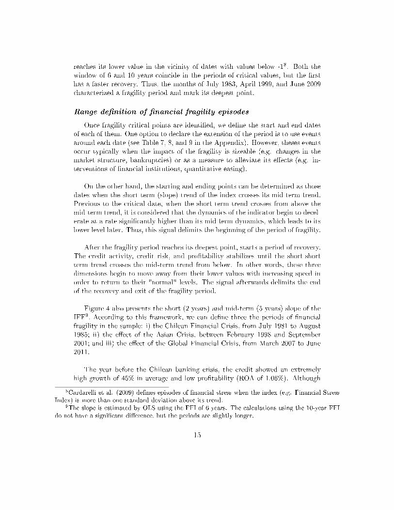
Table 2: Financial fragility periods ratios (mean)

Chilean �nancial crisis (July 1981 - July 1983 - August 1985)

Before Critical Fragility After

Jul.80 - Jun.81 Jul.83 Jul.81 - Aug.85 Sep.85 - Aug.86

Credit Growth 45,19 -4,76 7,43 -4,46

Past-due Index 1,63 13,22 7,28 4,32

ROA 1,06 -1,89 -0,66 0,29

Asian crisis (February 1998 - April 1999 - September 2001)

Before Critical Fragility After

Feb.97 - Jan.98 Apr.99 Feb.98 - Sep.01 Oct.01 - Sep.02

Credit Growth 12,24 0,49 5,34 4,56

Past-due Index 0,99 1,80 1,64 1,75

ROA 1,36 0,71 0,97 1,27

Global �nancial crisis (March 2007 - June 2009 - June 2011)

Before Critical Fragility After

Mar.06 - Feb.07 Jun.09 Mar.07 - Jun.11 Jul.11 - Jun.12

Credit Growth 14,60 -1,69 7,38 11,38

Past-due Index 0,81 1,26 1,05 1,05

ROA 1,26 1,04 1,19 1,29

The Asian crisis followed the same dynamic as the previous crisis. In thiscase, there was a deceleration of the credit growth from 12.2% to -0.2% in June1999, the past-due loans increased from 1% to 1.8% in April 1999 and continuedincreasing to 1.9% in June 2000. Although the returns on assets decreased to0.6% in this time, it recovered nearly its previous level.

Regarding the period of the global �nancial crisis, the credit growth showed amore severe contraction but a faster recovery than the asian crisis. On the otherhand, the past-due also increased, but its level and volatility were lower than theprevious fragility periods. In the same way, the pro�tability dropped to 0.9% in

16

October 2008, but returned to an average of 1.3%. In terms of levels and changeson this core variables, the local banking crisis was more severe.

5 Historical context of Chilean �nancial fragility

periods

In previous section, we identi�ed three periods of �nancial fragility over thelast 4 decades. This section describes the macroeconomic and �nancial contextsaround these episodes, highlighting signi�cant events that characterized �nancialvulnerability periods. Table 3 summarizes the main characteristics and causes ofthe delimited periods.

Table 3: Main characteristics and causes of �nancial fragility periods in Chile

Period Characteristics Causes

1982-1983 (external debt crisis) Insolvency of many institutions Financial liberalization

Increased credit risk Faults in regulation

Balance E�ects Credit Boom

Statization of banks Current account de�cits

1997-1999 (Asian crisis) Increased credit risk Current account de�cits

Reduction of pro�tability In�uence of capital

2007-2009 (global �nancial crisis) Increased credit risk Current account de�cits

Liquidity Restrictions In�uence of capital

Credit Restriction

5.1 Financial crisis 1982-1983

This is the only �nancial crisis period referred in the literature that is withinour time span (i.e. 1970-). It is often characterized among the ones that had thebiggest impact over a wide set of countries (Laeven & Valencia, 2008, 2012). Thissection analyzes the macroeconomic and �nancial conditions that originate andwere associated with this crisis.

Macroeconomic conditions

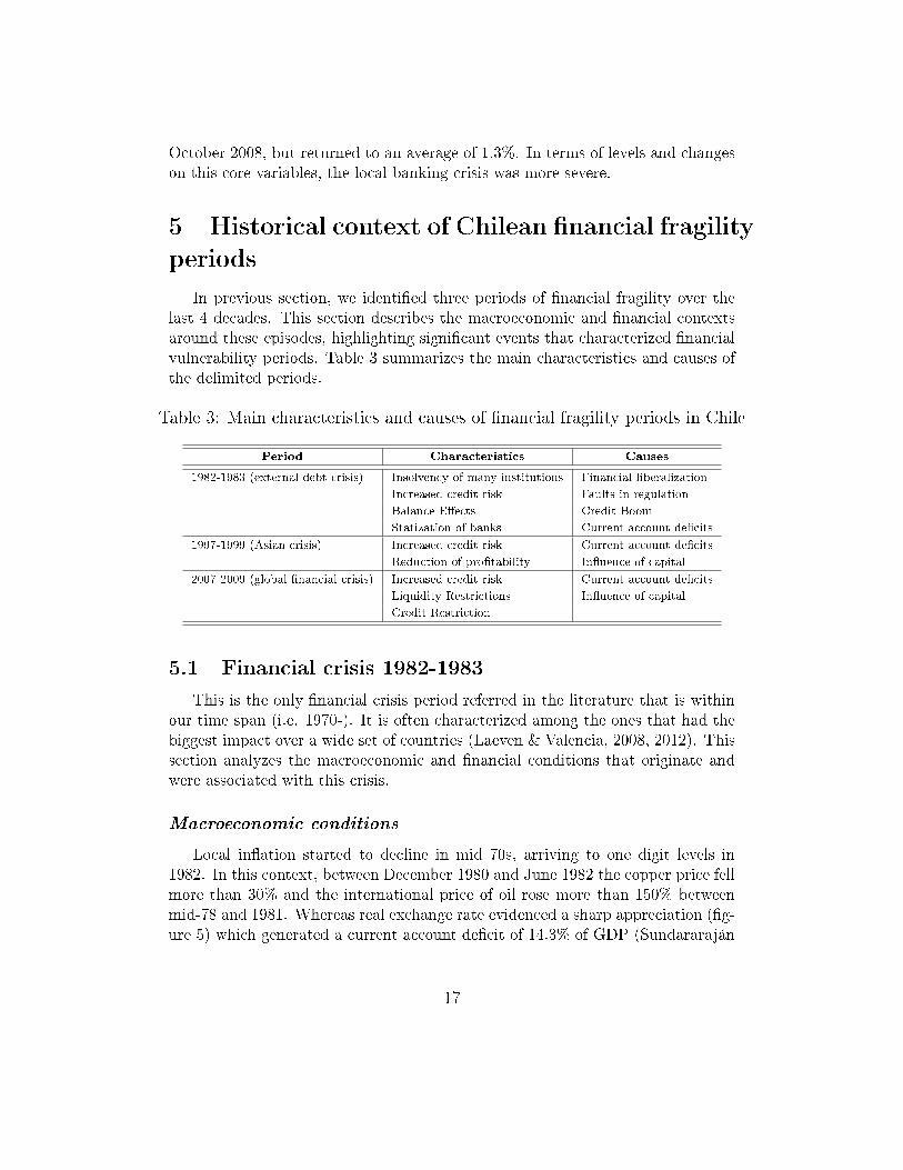
Local in�ation started to decline in mid 70s, arriving to one digit levels in1982. In this context, between December 1980 and June 1982 the copper price fellmore than 30% and the international price of oil rose more than 150% betweenmid-78 and 1981. Whereas real exchange rate evidenced a sharp appreciation (�g-ure 5) which generated a current account de�cit of 14.3% of GDP (Sundararaján

17

& Baliño, 1991; Caputo & Saravia, 2014).

Figure 5: Real Exchange Rate(1986 = 100)

50

65

80

95

110

125

Mar.79 Mar.83 Mar.87 Mar.91 Mar.95 Mar.99 Mar.03 Mar.07 Mar.11 Mar.15

Crisis Real exchange rate

The gray areas represent periods of �nancial fragility.Source: Own elaboration based on data from the CBC. Data before 1986 takenfrom Larrain & Vergara (2000) on annual basis.

As a consequence, terms of trade were deteriorated and forced a devaluationof the Chilean peso, changing the �xed exchange rate policy that was in forcebetween 1979 and 1982. Furthermore, in 1982 the country su�ered from an im-portant external capital sudden stop that further increased external vulnerabilities(Agosin y Huaita, 2012). In particular, in 1982 net capital in�ows were 64% lowerthan in the second half of the previous year.

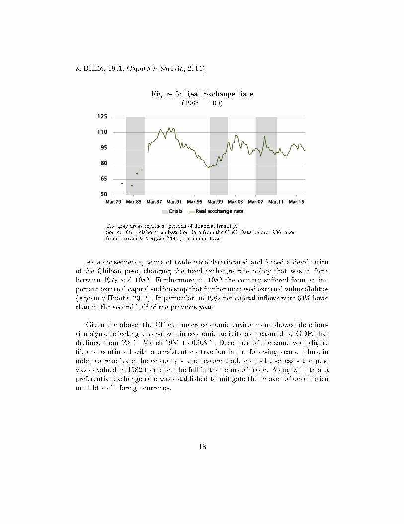
Given the above, the Chilean macroeconomic environment showed deteriora-tion signs, re�ecting a slowdown in economic activity as measured by GDP, thatdeclined from 9% in March 1981 to 0.9% in December of the same year (�gure6), and continued with a persistent contraction in the following years. Thus, inorder to reactivate the economy - and restore trade competitiveness - the pesowas devalued in 1982 to reduce the fall in the terms of trade. Along with this, apreferential exchange rate was established to mitigate the impact of devaluationon debtors in foreign currency.

18

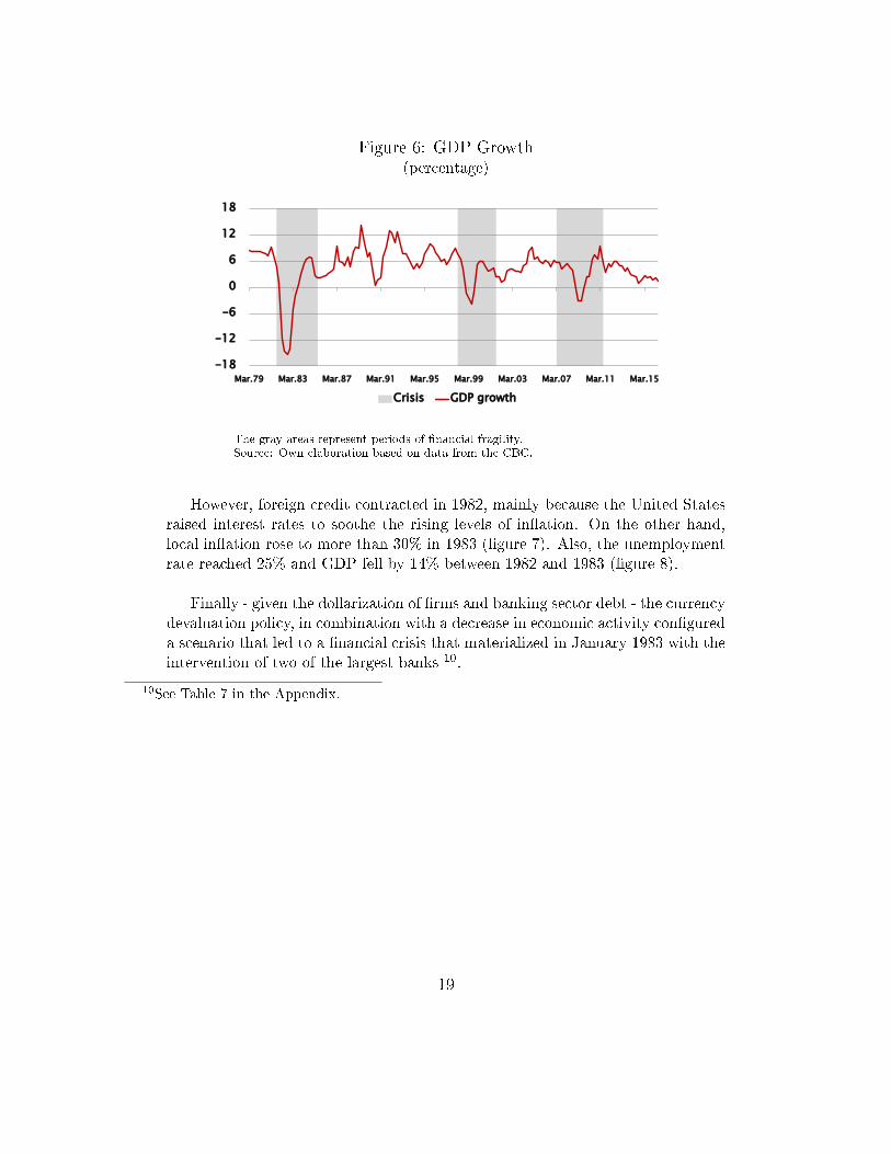
Figure 6: GDP Growth(percentage)

-18

-12

-6

0

6

12

18

Mar.79 Mar.83 Mar.87 Mar.91 Mar.95 Mar.99 Mar.03 Mar.07 Mar.11 Mar.15

Crisis GDP growth

The gray areas represent periods of �nancial fragility.Source: Own elaboration based on data from the CBC.

However, foreign credit contracted in 1982, mainly because the United Statesraised interest rates to soothe the rising levels of in�ation. On the other hand,local in�ation rose to more than 30% in 1983 (�gure 7). Also, the unemploymentrate reached 25% and GDP fell by 14% between 1982 and 1983 (�gure 8).

Finally - given the dollarization of �rms and banking sector debt - the currencydevaluation policy, in combination with a decrease in economic activity con�gureda scenario that led to a �nancial crisis that materialized in January 1983 with theintervention of two of the largest banks 10.

10See Table 7 in the Appendix.

19

Figure 7: In�ation(percentage)

-10

0

10

20

30

40

50

Mar.79 Mar.83 Mar.87 Mar.91 Mar.95 Mar.99 Mar.03 Mar.07 Mar.11 Mar.15

Crisis Inflation

The gray areas represent periods of �nancial fragility.Source: Own elaboration based on data from the CBC.

Figure 8: Unemployment Rate(percentage)

0

5

10

15

20

25

30

Mar.79 Mar.83 Mar.87 Mar.91 Mar.95 Mar.99 Mar.03 Mar.07 Mar.11 Mar.15

Crisis Gran Santiago unemployment rate

The gray areas represent periods of �nancial fragility.Source: Own elaboration based on data from the CBC.

Financial Environment

Since 1974, Chilean banking transited towards greater private sector partici-pation. It is also called a period of "�nancial liberalization" that sought to pro-

20

mote investment, savings and e�ciency in �nancial intermediation. At that time,quantitative controls and direct allocations of credit were eliminated, there wasa reduction in reserve rates and restrictions, the latter with the aim of allowingprivate banks to borrow in other countries. In addition, the market was opened to�nancial companies and foreign banks so that there would be greater competition.

As a result of the �nancial liberalization, bank credit grew strongly duringthis period in the second half of that decade. Credit operations of banks wereextended, changing from specialized to a multi-bank business type. On the otherhand, it started a process of privatization of banking entities, which were in thehands of CORFO. In addition, as of 1976, deposit reserve rates were reduced,which stabilized in 1980 at 10% for demand deposits and 4% for term deposits,which contributed to further increase the capacity to grant loans. Finally, this�nancial liberalization process was translated into a signi�cant increase in thenumber of banks, from 26 to 45 between 1978 and 1981 (of which 18 were for-eign), and a signi�cant increase in obligations with foreign banks.

Regarding the external situation, some developed countries increased interestrates in order to control the higher levels of in�ation derived from the rise inthe price of oil. This increase a�ected the payment capacity of companies andbanks that had borrowed abroad, which, added to the deterioration of the termsof trade, were important factors that triggered the economic crisis of the earlyeighties. Furthermore, this process was exacerbated because of the increased ex-posure of credit to non-tradable sectors (Brock, 1989). Additionally, the �nancialliberalization process was developed under a regulatory and supervisory frame-work that was not properly adapted to this growth of the banking system. Forexample, an important part of bank loans was used to �nance companies relatedto the bank's controlling group (Held & Jimenez, 1999).

As already noted, the policies taken to manage the crisis are mainly summa-rized in three: (i) assistance plans for local debtors, (ii) programs to strengthenthe banks solvency and (iii) policies to strengthen banking supervision (promotinga new General Banking Act).

Consequently, there was a fall in the past-due portfolio since 1985, an increasein the pro�tability indicators since 1986 and a decrease in the leverage level in thesame year. It should be noted that the SBIF allowed the banks to build up theshortfall in provisions for credit risk in the loan portfolio until the end of 1986.Government policies allowed to stabilize the economy, and in 1984 GDP reversedthe decline of previous years. This, along with the plans taken to regularize thebanking system, permitted the industry to improve its �nancial situation. In

21

this way, since 1985, there was a fall in the past-due portfolio, an increase in thepro�tability indicators since 1986 and a decrease in the level of leverage in sameyear. The SBIF helped the banks to build up the shortfall in provisions for creditrisk in the loan portfolio until the end of 1986. In order to strength the position ofthe �nancial system, in November 1986 the General Law on Banks was modi�ed,which improved the weaker aspects of previous legislation (Held & Jimenez, 1999).

5.2 Asian Crisis 1997-1999

Unlike the local banking crisis, this period was largely attributable to externalfactors that reversed the period of high economic expansion that the countrylived in the period 1984-1997 with an average GDP growth of 7.1% per annum,the highest from the country's independency (De Gregorio, 2005).

Macroeconomic conditions

The main e�ects of the Asian crisis were re�ected in the unfavorable resultsof foreign trade, due to Chile's high dependence on international markets and therelatively low diversi�cation of its export goods and destinations. Indeed, thedeterioration of the terms of trade (4.8% for 1998) are mainly explained by thefall in exports. As a consequence of the above, in the last quarter of 1997 thecurrent account de�cit was around 4,000 billion, equivalent to 5% of GDP (�gure6). Also, this economic crisis had an impact on local economic activity, whichregistered a fall of 0.9% of GDP and an increase in unemployment that exceeded10% in 1999 (�gure 8), and was exacerbated - in a context of exchange rate bandpolicy - by a monetary adjustment that almost doubled the real annual interestrate from 8.5% to 14%.

Financial environment

The Asian crisis impact on the banking system was limited in terms of insol-vencies. This was largely due to policies that were implemented before, such asthe General Banking Act (or "Ley General de Bancos" in Spanish) and modi�ca-tions made in 1986 and 1997 (the Basel framework was included in 1997). Thesechanges made it possible to reduce the impact of the deterioration of the capacityof companies and households in the past-due portfolio indicators, in spite of thedrop in economic activity and the increase in unemployment already indicated.During the 90's changes provisions regulation were combined with an explosiveincrease in consumer credit, given �exible lending policies. This situation ended inhigher levels of write-o�s (reached 1.3% in 1999, from 0.9% in 1997) and past-dueloans (reached 1.8% in 1999, from 1.0% in 1997). However, pro�tability indicators

22

were the most a�ected ones. In fact, in 1999 ROA and ROE reached the lowestlevels in 30 years (0.7 and 9.4%, respectively), caused mainly by the increase inthe cost of loan loss provisions, because of increased credit risk.

Although important, as compared to the previous crisis, this episode had amoderate impact on the growth rate of banking credit. Indeed, commercial lend-ing registered almost zero growth in mid-1999, while consumer lending showed anattenuated fall. Housing loans grew sharply in the 1990s as a result of the massivedevelopment of non-endorsable mortgage loans, low interest rates and the sharpincrease in mortgages loan-to-value to �nance properties of up to 100%.

On the other hand, the leverage remained stable in this period. Given theimplementation of the capital adequacy ratio (CAR) - under Basel I criteria thatwas present in the General Banking Act - banks increased their capital by morethan 7% in 1999. Hence, the CAR rose from 11.04% in December 1998 to 13.50%in December 1999.

5.3 Global Financial Crisis (2007-2009)

As in the Asian crisis fragility period, the Global Financial Crisis episode wasoriginated, to a large extent, by external factors that a�ected the external �nancialposition. These factors are related to a sharp reduction in global liquidity andthe investors �ight to quality that prevailed between 2007 and 2008, and wastranslated in local credit restrictions (Claessens et al., 2010).

Macroeconomic Environment

The current account su�ered a reversal of more than 6 points of GDP in 2008compared to the previous year, reaching a de�cit of 2.4% of GDP (�gure 9).

23

Figure 9: GDP Growth and Current Account De�cit.(percentage)

-15

-10

-5

0

5

10

15

78 82 86 90 94 98 02 06 10 14

Current Account Deficit Anual GDP Growth

The gray areas represent periods of �nancial fragility.Source: Own elaboration based on data from the CBC.

The copper price that represented 50% of exports in those years fell to $1.4per pound during the crisis. It was equivalent to a decline of more than 50%in 2008. The local loans interest rate in dollars increased more than 300 bp inOctober 2008. Moreover, there was a drop in the demand for Chilean exports(goods and services exports fell more than 6% in 2009). Also, between 2008 and2009 the national unemployment rate increased from 7.8% to over 10% (�gure 9)and the domestic demand fell 8% in the �rst half of that year as compared tothe same period in 2008. Additionally, the GDP turned from an annual growthslightly above 5% in 2008 to a contraction of 3% in the second half of 2009.

Financial Environment

The volatility that characterized this period generated a greater preference forliquidity, which triggered an increase in interest rates in the local �nancial market(Financial Stability Report, First Half 2009). The spread between the local loaninterest rate in the foreign currency and the LIBOR rate increased around 100bp,between May and September 2008, a situation that also had an impact on therates of loans and funding in pesos (Financial Stability Report, Second Half 2008).

Since the last quarter of 2008, the banking credit growth decelerated (partic-ularly for consumer and commercial portfolios). On the other hand, the credit

24

risk increased. Thus, both the past-due loans ratio and loan loss provisions in-creased by approximately 50bp between 2008 and 2009. Accordingly, the bakingsystem tighten its credit standards and the credit demand decreased, particularlyfor consumer loans (BCCh ECB report, 2008).

Pro�tability was less a�ected than in the Asian crisis, and reached its lowestlevel in early 2009 (12% ROE) but recovered the average of the last 5 years atthe beginning of 2010 because of both the more expansive monetary policy andlong-term liquidity facilities (FLAP). The latter helped to reduce the bank's costof funds and increase the pro�t from treasury operations.

The banks solvency increased in the period. Between October 2008 and De-cember 2009, both the leverage and the capital adequacy ratio increased by morethan 50 and 250 basis points, respectively. Mainly, due to risk-weighted assetsreduction (9% in the same period).

6 Final remarks

In this paper we have shown that the Chilean �nancial fragility periods canbe identi�ed by using a small set of variables that describe the banking sectorperformance and risks. In this respect, this is the �rst paper in attempting tocharacterizing the Chilean �nancial cycle. To accomplish that, we do a review ofthe literature and select a group of ratios following a precise rationale. Accord-ingly, we build a database that extends those �nancial variables back to the 70's,and process this information, developing a composite index that delimits �nancialfragility periods.

Also, we illustrate the �nancial cycle and fragility periods by introducing a se-ries of indicators of macroeconomic performance, and external/internal �nancialposition. By assuming that historic patterns will repeat in the future in a similarfashion, this analysis enables us to extract policy lessons from past macroeconomicand �nancial regulatory frameworks.

We propose the use of the analysis and conclusions of this work for �nancialpolicy design and implementation, especially, for the banking sector. In particular,in Chilean case, our results allow policy makers to test anticipative propertiesof early warning indicators that are introduced by the contemporaneous macro-prudential framework, such as the CCyB.

25

References

[1] Agosin, M., and Huaita, F. Overreaction in capital �ows to emergingmarkets: Booms and sudden stops. Journal of International Money and

Finance, 31 (2012), 1140�1155.[2] Ahumada, A., and Budnevich, C. Some measures of �nancial fragility in

the chilean banking system: An early warning indicators application. Serieson Central Banking, Analysis, and Economic Policies 3 (2002), 303�332.

[3] Albertazzi, U., and Gambacorta, L. Bank pro�tability and the businesscycle. Journal of Financial Stability 5, 4 (2009), 393�409.

[4] Allen, F., and Gale, D. Financial fragility, liquidity, and asset prices.Journal of the European Economic Association 2, 6 (2004), 1015�1048.

[5] Amieva, J., and Urriza, B. Liberalización �nanciera, crisis y reforma delsistema bancario chileno: 1974�1999. Política �scal, 108 (2000).

[6] Bell, J., and Pain, D. Leading indicator models of banking crises�a criticalreview. Financial Stability Review 9 (2000), 113�129.

[7] Bordo, M. D., Dueker, M. J., and Wheelock, D. C. Aggregate priceshocks and �nancial instability: A historical analysis. Economic Inquiry 40,4 (2002), 521�538.

[8] Borio, C. The �nancial cycle and macroeconomics: What have we learnt?Journal of Banking & Finance 45 (2014), 182�198.

[9] Borio, C., and Drehmann, M. Assessing the risk of banking crises�revisited. BIS Quarterly Review (2009).

[10] Brock, P. L. La crisis �nanciera chilena. Cuadernos de Economía 26, 78(1989), 177�194.

[11] Brunnermeier, M. K., and Schnabel, I. Bubbles and Central Banks:

Historical Perspectives. Cambridge University Press, Cambridge, UK, 2016.[12] Caputo, R., and Saravia, D. The �scal and monetary history of chile

1960�2010. Becker Friedman Working Papers (2014).[13] Cardarelli, R., Elekdag, S., and Lall, S. Financial stress, downturns,

and recoveries. IMF Working Paper, WP/09/100 (2009).[14] Central Bank of Chile. Financial stability report, several numbers.[15] Central Bank of Chile. Indicadores economicos y sociales de chile 1960�

2000. Santiago de Chile, 2001.[16] Claessens, S., and Kose, M. A. Financial crises explanations, types, and

implications. IMF Working Paper, 13/28 (2013).[17] De Gregorio, J. Crecimiento económico en chile: Evidencia, fuentes y

perspectivas. Estudios Públicos, 98 (2005), 19�86.[18] De Gregorio, J. Chile and the global recession of 2009. Documentos de

Política Económica, 30 (2009).

26

[19] Demirgüç-Kunt, A., and Detragiache, E. The determinants of bank-ing crises-evidence from industrial and developing countries. Policy ResearchWorking Paper, WPS1828 (1997).

[20] Demirgüç-Kunt, A., and Detragiache, E. Monitoring banking sectorfragility: a multivariate logit approach. IMF Working Paper, WP/99/147(1999).

[21] Detken, C., Weeken, O., Alessi, L., Bonfim, D., Boucinha, M. M.,

Castro, C., Frontczak, S., Giordana, G., Giese, J., Jahn, N.,

et al. Operationalising the countercyclical capital bu�er: indicator selec-tion, threshold identi�cation and calibration options. ESRB Occasional paper

5 (2014).[22] Edison, H. J. Do indicators of �nancial crises work? an evaluation of an

early warning system. International Journal of Finance & Economics 8, 1(2003), 11�53.

[23] Eichengreen, B., Rose, A. K., and Wyplosz, C. Contagious currencycrises. Tech. rep., National bureau of economic research, 1996.

[24] Federal Reserve Bank of Chicago. Background on the chicago fednational activity index. Background Information (2016).

[25] Federal Reserve Bank of San Francisco. The search for �nancialstability: The past �fty years. Proceedings of a Conference held June 23�25

(1985).[26] Gadanecz, B., Jayaram, K., et al. Measures of �nancial stability-a

review. IFc bulletin 31 (2009), 365�380.[27] Goldstein, M., Kaminsky, G., and Reinhart, C. Assessing �nancial

vulnerability, an early warning system for emerging markets: Introduction.MPRA Paper, 13629 (2000).

[28] Goldstein, M., and Reinhart, C. Assessing Financial Vulnerability:

An Early Warning System for Emerging Markets. Peterson Institute forInternational Economics, 2000.

[29] Goodhart, C. The conduct of monetary policy. The Economic Journal 99,396 (1989), 293�346.

[30] Goodhart, C. A. Price stability and �nancial fragility. In Financial stabilityin a changing environment. Springer, 1995, pp. 439�509.

[31] Goodhart, C. A., Sunirand, P., and Tsomocos, D. P. A model toanalyse �nancial fragility. Economic Theory 27, 1 (2006), 107�142.

[32] Guttentag, J., and Herring, R. Credit rationing and �nancial disorder.The Journal of Finance 39, 5 (1984), 1359�1382.

[33] Hausmann, R., and Rojas�Suárez, L. Las crisis bancarias en América

Latina. Fondo de Cultura Económica, 1997.

27

[34] Held, G., and Jiménez, L. F. Liberalización �nanciera, crisis y reformadel sistema bancario chileno: 1974�1999. Financiamiento del desarrollo, 90(1999).

[35] Illing, M., and Liu, Y. An index of �nancial stress for canada. Tech. rep.,2003.

[36] Kaminsky, G. L. Currency and banking crises: the early warnings of dis-

tress. No. 99-178. International Monetary Fund, 1999.[37] Kaminsky, G. L., and Reinhart, C. M. The twin crises: the causes

of banking and balance-of-payments problems. American economic review

(1999), 473�500.[38] Kruger, M., Osakwe, P. N., and Page, J. Fundamentals, contagion

and currency crises: an empirical analysis. Development Policy Review 18, 3(2000), 257�274.

[39] Laeven, L., and Valencia, F. Systemic banking crises: a new database.Working Paper, 08/224 (2008).

[40] Laeven, L., and Valencia, F. Systemic banking crises database: Anupdate. Working Paper, 12/163 (2012).

[41] Larraín, F., and Vergara, R. La Transformación Económica de Chile.Centro de Estudios Públicos, 2000.

[42] Lim, C. H., Klemm, A. D., Ogawa, S., Pani, M., and Visconti, C.

Financial Stability Reports in Latin America and the Caribbean. InternationalMonetary Fund, 2017.

[43] Logan, A. The united kingdom's small banks' crisis of the early 1990s:What were the leading indicators of failure? Bank of England Working

Paper, 139 (2001).[44] Manikow, N. G. The allocation of credit and �nancial collapse. Cambridge,

Massachusetts: NBER Working Paper, 1786 (1986).[45] Merton, R. On the pricing of corporate debt: The risk structure of interest

rates. The Journal of Finance 29 (1974).[46] Merton, R. C. On the pricing of corporate debt: The risk structure of

interest rates. The Journal of �nance 29, 2 (1974), 449�470.[47] Minsky, H. P. An evaluation of recent monetary policy. Nebraska Journal

of Economics and Business (1972), 37�56.[48] Miron, J. A. Financial panics, the seasonality of the nominal interest rate,

and the founding of the fed. The American Economic Review 76, 1 (1986),125�140.

[49] Mitchell, W. C. Business cycles and their causes. University of CaliforniaPress (1941).

[50] Reinhart, C. M., and Rogoff, K. S. This time is di�erent: Eight cen-

turies of �nancial folly. Princeton University Press, 2009.

28

[51] Schwartz, A. J. Real and pseudo �nancial crises. Financial Crises in the

World Banking System (1985).[52] Shin, H. S. Procyclicality and the search for early warning indicators. IMF

Working Paper, WP/13/258 (2013).[53] Stiglitz, J. E., and Weiss, A. Credit rationing in markets with imperfect

information. The American economic review 71, 3 (1981), 393�410.[54] Stock, J. H., and Watson, M. W. Forecasting in�ation. Journal of

Monetary Economics 44, 2 (1999), 293�335.[55] Sundararajan, V., and Baliño, T. Banking Crises : Cases and Issues.

International Monetary Fund, March 1991.[56] Veblen, T. The theory of business enterprise. C. Scribner's sons, 1904.[57] Wolfson, M. Financial crises: Understanding the postwar u.s. experience.

M.E. Shoope, Inc (1986).

29

7 Appendix

7.1 Data construction criteria

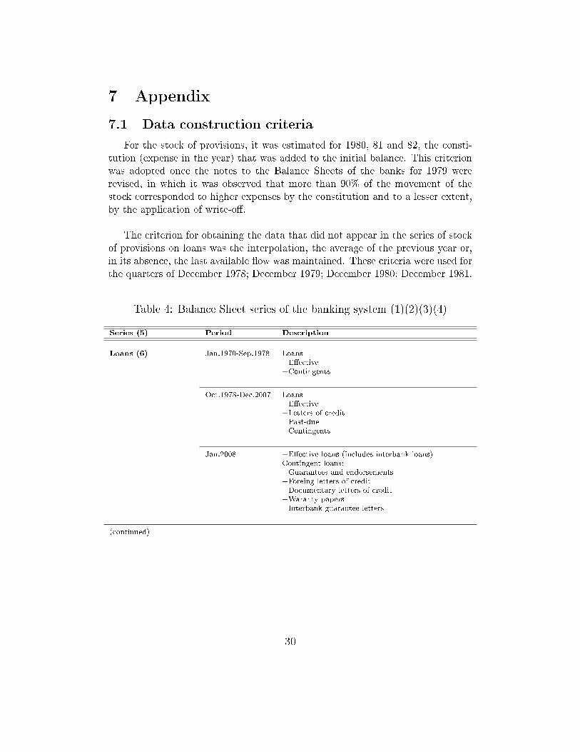
For the stock of provisions, it was estimated for 1980, 81 and 82, the consti-tution (expense in the year) that was added to the initial balance. This criterionwas adopted once the notes to the Balance Sheets of the banks for 1979 wererevised, in which it was observed that more than 90% of the movement of thestock corresponded to higher expenses by the constitution and to a lesser extent,by the application of write-o�.

The criterion for obtaining the data that did not appear in the series of stockof provisions on loans was the interpolation, the average of the previous year or,in its absence, the last available �ow was maintained. These criteria were used forthe quarters of December 1978; December 1979; December 1980; December 1981.

Table 4: Balance Sheet series of the banking system (1)(2)(3)(4)

Series (5) Period Description

Loans (6) Jan.1970-Sep.1978 Loans+E�ective+Contingents

Oct.1978-Dec.2007 Loans+E�ective+Letters of credit+Past-due+Contingents

Jan.2008- +E�ective loans (includes interbank loans)Contingent loans:+Guarantees and endorsements+Foreing letters of credit+Documentary letters of credit+Waranty papers+Interbank guarantee letters

(continued)

30

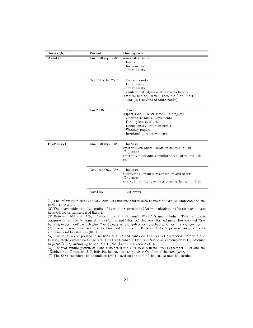
Series (5) Period Description

Assets Jan.1970-sep.1978 +Available funds+Loans+Investments+Other assets

Oct.1978-Dec.2007 +Current assets+Fixed assets+Other assets+Control and adjustment accounts (assets)-Control and adjustment accounts (liabilities)-Float (instruments of other banks)

Jan.2008- +Assets-Operations with settlement in progress+Guarantees and endorsements+Foreing letters of credit+Documentary letters of credit+Waranty papers+Interbank guarantee letters

Pro�ts (7) Jan.1970-sep.1978 +Income:Interests, discounts, commissions and others-Expenses:Interests, discounts, commissions, salaries and oth-ers

Oct.1978-Oct.1982 +Income:Operational, monetary correction and others-Expenses:Operational, �xed, monetary correction and others

Nov.1982- +Net pro�t

(1) The information since January 2008 uses unconsolidated data to make the series comparable to theperiod 1970-2017.(2) The unavailable data (i.e. pro�ts of June and September 1972) were obtained by its ratio over loansinterpolated or extrapolated linearly.(3) Between 1975 and 1978, information on the "Financial Firms" is not included. This group wascomposed of non-bank �nancial �rms (formal and informal) that were formed under the so-called "freebanking experiment", which after 2 or 3 years were dissolved or absorbed by other �nancial entities.(4) The source of information is the Financial Information Bulletin of the Superintendency of Banksand Financial Institutions (SBIF).(5) The series are expressed in millions of CLP and considers the total of currencies (domestic andforeign) at the currect exchange rate. Until September of 1975, the "escudos" currency were transformedto pesos (CLP), according to the rate 1 peso ($) = 1 000 escudos (E).(6) The real annual growth of loans considered the CPI as a de�ator until September 1979 and the"Unidades de Fomento" (UF, in�ation indexed currency) since October of the same year.(7) The ROA considers the annualized pro�t based on the sum of the last 12 monthly results.

31

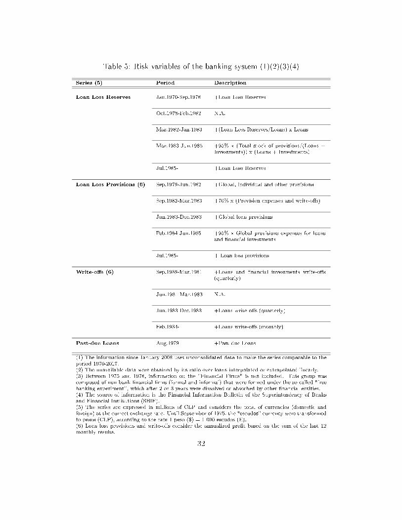
Table 5: Risk variables of the banking system (1)(2)(3)(4)

Series (5) Period Description

Loan Loss Reserves Jan.1970-Sep.1978 +Loan Loss Reserves

Oct.1978-Feb.1982 N.A.

Mar.1982-Jan.1983 +(Loan Loss Reserves/Loans) x Loans

Mar.1983-Jun.1985 +95% x (Total stock of provisions/(Loans +Investments)) x (Loans + Investments)

Jul.1985- +Loan Loss Reserves

Loan Loss Provisions (6) Sep.1979-Jun.1982 +Global, individual and other provisions

Sep.1982-Mar.1983 +70% x (Provision expenses and write-o�s)

Jun.1983-Dec.1983 +Global loan provisions

Feb.1984-Jun.1985 +95% x Global provisions expenses for loansand �nancial investments

Jul.1985- + Loan loss provisions

Write-o�s (6) Sep.1989-Mar.1981 +Loans and �nancial investments write-o�s(quarterly)

Jun.1981-Mar.1983 N.A.

Jun.1983-Dec.1983 +Loans write-o�s (quarterly)

Feb.1984- +Loans write-o�s (monthly)

Past-due Loans Aug.1979- +Past-due Loans

(1) The information since January 2008 uses unconsolidated data to make the series comparable to theperiod 1970-2017.(2) The unavailable data were obtained by its ratio over loans interpolated or extrapolated linearly.(3) Between 1975 and 1978, information on the "Financial Firms" is not included. This group wascomposed of non-bank �nancial �rms (formal and informal) that were formed under the so-called "freebanking experiment", which after 2 or 3 years were dissolved or absorbed by other �nancial entities.(4) The source of information is the Financial Information Bulletin of the Superintendency of Banksand Financial Institutions (SBIF).(5) The series are expressed in millions of CLP and considers the total of currencies (domestic andforeign) at the currect exchange rate. Until September of 1975, the "escudos" currency were transformedto pesos (CLP), according to the rate 1 peso ($) = 1 000 escudos (E).(6) Loan loss provisions and write-o�s consider the annualized pro�t based on the sum of the last 12monthly results.

32

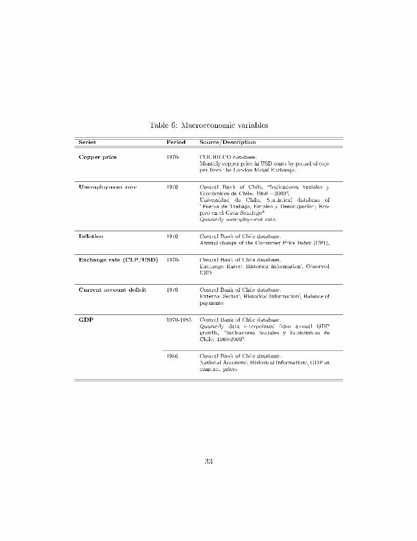
Table 6: Macroeconomic variables

Series Period Source/Description

Copper price 1970- COCHILCO database.Monthly copper price in USD cents by pound of cop-per from the London Metal Exchange.

Unemployment rate 1970- Central Bank of Chile, �Indicadores Sociales yEconómicos de Chile: 1960 � 2000�.Universidad de Chile, Statistical database of"Fuerza de Trabajo, Empleo y Desocupación; Em-pleo en el Gran Santiago"Quarterly unemployment rate.

In�ation 1970- Central Bank of Chile database.Annual change of the Consumer Price Index (CPI).

Exchange rate (CLP/USD) 1970- Central Bank of Chile database.Exchange Rates\ Historica Information\ ObservedUSD

Current account de�cit 1970- Central Bank of Chile database.External Sector\ Historical Information\ Balance ofpayments

GDP 1970-1985 Central Bank of Chile database.Quarterly data interpolated from annual GDPgrowth, "Indicadores Sociales y Económicos deChile: 1960-2000�.

1986- Central Bank of Chile database.National Accounts\ Historical Information\ GDP atconstant prices

33

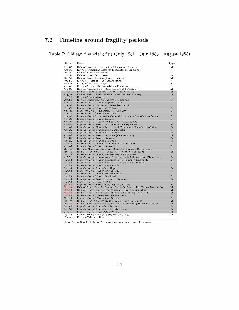
7.2 Timeline around fragility periods

Table 7: Chilean �nancial crisis (July 1981 - July 1983 - August 1985)

Date Event Type

Apr.80 Exit of Banco Consititución (Banco A. Edwards) MApr.80 Entry of American Express International Banking SMay.80 Exit of Financiera Melón EJul.80 Exit of Financiera Tasco EOct.80 Exit of Banco Curicó (Banco Nacional) MDec.80 Entry of Chicago Continental Bank SMar.81 Entry of Bank of Tokyo SApr.81 Entry of Banco Empresarial de Fomento SApr.81 Exit of Agrobanco de Chile (Banco del Pací�co) MJul.81 Exit of Banco Israelita (Banco Internacional) MAug.81 Exit of Banco Regional de Linares (Banco Linares) MSep.81 Entry of Centrobanco SOct.81 Exit of Financiera de Papeles y Cartones ENov.81 Intervention of Banco Español-Chile INov.81 Intervention of Sociedad Financiera del Sur INov.81 Intervention of Banco de Talca INov.81 Intervention of Financiera de Capitales INov.81 Intervention of Financiera Cash INov.81 Intervention of Compañía General Financiera Sociedad Anónima INov.81 Intervention of Banco Linares INov.81 Intervention of Banco de Fomento de Valparaíso IApr.82 Liquidation of Banco de Fomento de Valparaíso EApr.82 Liquidation of Compañía General Financiera Sociedad Anónima EApr.82 Liquidation of Financiera de Capitales EApr.82 Liquidation of Financiera del Sur EApr.82 Liquidation of Banco de Talca (Centrobanco) MApr.82 Liquidation of Banco Linares EApr.82 Liquidation of Financiera Cash EApr.82 Intervention of Banco de Fomento del Bío-Bío IApr.82 Intervention of Banco Austral IMay.82 Entry of The Hongkong and Shanghai Banking Corporation SMay.82 Exit of Financiera de Los Andes (Banco A. Edwards) MJun.82 Intervention of Banco Empresarial de Fomento IJul.82 Liquidation of Adelantos y Créditos Sociedad Anónima Financiera EJan.83 Intervention of Banco Hipotecario de Fomento Nacional. IJan.83 Intervention of Banco Colocadora Nacional de Valores IJan.83 Intervention of Banco Concepción IJan.83 Liquidation of Financiera Ciga EJan.83 Intervention of Banco de Santiago IJan.83 Intervention of Banco Internacional IJan.83 Intervention of Banco Nacional IJan.83 Liquidation of Banco Unido de Fomento EJan.83 Intervention of Banco de Chile IJan.83 Liquidation of Banco Hipotecario de Chile EFeb.83 Exit of Financiera Latinoamericana de Desarrollo (Banco Desarrollo) MFeb.83 Exit of Financiera de Interés Social (Banco Desarrollo) MFeb.83 Exit of Banco Empresarial de Fomento (Banco Desarrollo) MJan.85 Intervention of Financiera Mediterráneo IFeb.85 Intervention of Financiera Davens IMar.85 Exit of Financiera Cor�nsa (Banco Sud Americano) MMay.85 Exit of Banco Colocadora Nacional de Valores (Banco Santiago) MJun.85 Liquidation of Financiera Davens EJun.85 Liquidation of Financiera Mediterráneo EJul.85 Intervention of Financiera Davens EOct.85 Exit of Morgan Finansa (Banco de Chile) MNov.85 Entry of Morgan Bank S

1 S = Entry, E = Exit, M = Merge and Adquisitions, I = Intervention.

34

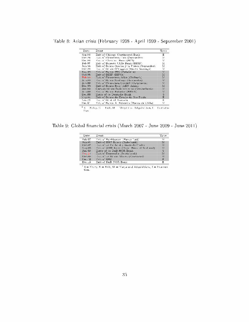
Table 8: Asian crisis (February 1998 - April 1999 - September 2001)

Date Event Type

Sep.94 Exit of Chicago Continental Bank EDec.94 Exit of Financiera Fusa (Santander) MDec.94 Exit of Chemical Bank (BCI) MFeb.95 Exit of Banesto Chile Bank (BHIF) MJun.96 Exit of Banco Osorno y la Union (Santander) MDec.96 Exit of Banco O'Higgins (Banco Santiago) MAug.98 Exit of Banco ING (Falabella) MOct.98 Exit of BHIF (BBVA) MFeb.99 Exit of Financiera Atlas (Citibank) MJun.99 Exit of Banco Santiago (Santander) MJun.99 Exit of Financiera Condell (Corpbanca) MDec.99 Exit of Banco Real (ABN Amro) MJan.00 Cambio Banco Sudamericano (Scotianbank) MJun.00 Exit of Banco Exterior (BBVA) MDec.00 Entry of de Deutsche Bank SMay.01 Exit of Banco do Estado do Sao Paulo ENov.01 Exit of Bank of America EDec.01 Exit of Banco A. Edwards (Banco de Chile) M

1 S = Entry, E = Exit, M = Merge and Adquisitions, I = Interven-tion.

Table 9: Global �nancial crisis (March 2007 - June 2009 - June 2011)

Date Event Type

Feb.07 Exit of Bankboston (Banco Itaú) MJun.07 Exit of HNS Banco (Rabobank) MDec.07 Exit of de Citibank (Banco de Chile) MMay.08 Exit of ABN Amro (Royal Bank of Scotland) MJan.09 Entry of de DnB NOR Bank SNov.09 Exit of Desarrollo (Scotiabank) MDec.09 Exit of de Banco Monex (Consorcio) MDec.10 Exit of RBS EDec.12 Exit of DnB NOR Bank E

1 S = Entry, E = Exit, M = Merge and Adquisitions, I = Interven-tion.

35

Documentos de Trabajo

Banco Central de Chile

NÚMEROS ANTERIORES

La serie de Documentos de Trabajo en versión PDF puede obtenerse gratis en la dirección electrónica: www.bcentral.cl/esp/estpub/estudios/dtbc. Existe la posibilidad de solicitar una copia impresa con un costo de Ch$500 si es dentro de Chile y US$12 si es fuera de Chile. Las solicitudes se pueden hacer por fax: +56 2 26702231 o a través del correo electrónico: bcch@bcentral.cl.

Working Papers

Central Bank of Chile

PAST ISSUES

Working Papers in PDF format can be downloaded free of charge from: www.bcentral.cl/eng/stdpub/studies/workingpaper. Printed versions can be ordered individually for US$12 per copy (for order inside Chile the charge is Ch$500.) Orders can be placed by fax: +56 2 26702231 or by email: bcch@bcentral.cl.

DTBC – 821 Pension Funds and the Yield Curve: the role of Preference for Maturity Rodrigo Alfaro y Mauricio Calani DTBC – 820 Credit Guarantees and New Bank Relationships

William Mullins y Patricio Toro DTBC – 819 Asymmetric monetary policy responses and the effects of a rise in the inflation target

Benjamín García DTBC – 818 Medida de Aversión al Riesgo Mediante Volatilidades Implícitas y Realizadas

Nicolás Álvarez, Antonio Fernandois y Andrés Sagner DTBC – 817 Monetary Policy Effects on the Chilean Stock Market: An Automated Content

Approach Mario González y Raúl Tadle DTBC – 816 Institutional Quality and Sovereign Flows

David Moreno DTBC – 815 Desarrollo del Crowdfunding en Chile

Iván Abarca DTBC – 814 Expectativas Financieras y Tasas Forward en Chile

Rodrigo Alfaro, Antonio Fernandois y Andrés Sagner DTBC – 813 Identifying Complex Core-Periphery Structures in the Interbank Market

José Gabriel Carreño y Rodrigo Cifuentes DTBC – 812 Labor Market Flows: Evidence for Chile Using Micro Data from Administrative Tax

Records Elías Albagli, Alejandra Chovar, Emiliano Luttini, Carlos Madeira, Alberto Naudon, Matías Tapia DTBC – 811 An Overview of Inflation-Targeting Frameworks: Institutional Arrangements,

Decision-making, & the Communication of Monetary Policy Alberto Naudon y Andrés Pérez DTBC – 810 How do manufacturing exports react to RER and foreign demand? The Chilean case

Jorge Fornero, Miguel Fuentes y Andrés Gatty DTBC – 809 A Model of Labor Supply, Fixed Costs and Work Schedules

Gonzalo Castex y Evgenia Detcher DTBC – 808 Dispersed Information and Sovereign Risk Premia

Paula Margaretic y Sebastián Becerra DTBC – 807 The Implications of Exhaustible Resources and Sectoral Composition for Growth

Accounting: An Application to Chile

Claudia De La Huerta y Emiliano Luttini DTBC – 806 Distribución de Riqueza No Previsional de los Hogares Chilenos

Felipe Martínez y Francisca Uribe

DOCUMENTOS DE TRABAJO • Junio 2018