DISTRIBUTION OF VEHICLE SPEEDS AND TRAVEL TIMES

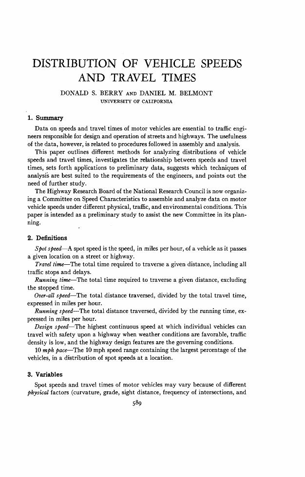
DISTRIBUTION OF VEHICLE SPEEDSAND TRAVEL TIMES

DONALD S. BERRY AND DANIEL M. BELMONTUNIVERSITY OF CALIFORNIA

1. SummaryData on speeds and travel times of motor vehicles are essential to traffic engi-

neers responsible for design and operation of streets and highways. The usefulnessof the data, however, is related to procedures followed in assembly and analysis.

This paper outlines different methods for analyzing distributions of vehiclespeeds and travel times, investigates the relationship between speeds and traveltimes, sets forth applications to preliminary data, suggests which techniques ofanalysis are best suited to the requirements of the engineers, and points out theneed of further study.

The Highway Research Board of the National Research Council is now organiz-ing a Committee on Speed Characteristics to assemble and analyze data on motorvehicle speeds under different physical, traffic, and environmental conditions. Thispaper is intended as a preliminary study to assist the new Committee in its plan-ning.

2. DefinitionsSpot speed-A spot speed is the speed, in miles per hour, of a vehicle as it passes

a given location on a street or highway.Travel time-The total time required to traverse a given distance, including all

traffic stops and delays.Running time-The total time required to traverse a given distance, excluding

the stopped time.Over-all speed-The total distance traversed, divided by the total travel time,

expressed in miles per hour.Running speed-The total distance traversed, divided by the running time, ex-

pressed in miles per hour.Design speed-The highest continuous speed at which individual vehicles can

travel with safety upon a highway when weather conditions are favorable, trafficdensity is low, and the highway design features are the governing conditions.

10 mph pace-The 10 mph speed range containing the largest percentage of thevehicles, in a distribution of spot speeds at a location.

3. Variables

Spot speeds and travel times of motor vehicles may vary because of differentphysical factors (curvature, grade, sight distance, frequency of intersections, and

589

590 SECOND BERKELEY SYMPOSIUM: BERRY AND BELMONT

roadside development), different traffic factors (volume of traffic, percent ofthrough traffic, turning traffic, proportion of trucks, parking conditions, and vol-ume of pedestrians), and different environmental factors (section of the country,driVer characteristics, weather, season, visibility, enforcement practices, speedlimits, and other traffic controls).

The speed characteristics at any one location may change from time to time be-cause of the effect of one or more factors such as changes in traffic volumes,weather, or visibility. Speeds may also change as the result of changes or a com-bination of changes in speed limits, parking regulations, enforcement, or othertraffic control measures.

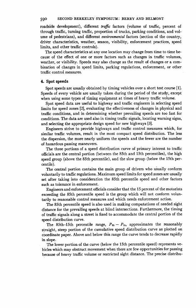
4. Spot speeds

Spot speeds are usually obtained by timing vehicles over a short test course [1].Speeds of every vehicle are usually taken during the period of the study, exceptwhen using some types of timing equipment at times of heavy traffic volume.

Spot speed data are useful to highway and traffic engineers in selecting speedlimits for speed zones 12], evaluating the effectiveness of changes in physical andtraffic conditions, and in determining whether prevailing speeds are too fast forconditions. The data are used also in timing traffic signals, locating warning signs,and selecting the appropriate design speed for new highways [3].

Engineers strive to provide highways and traffic control measures which, forsimilar traffic volumes, result in the most compact speed distribution. The lessthe dispersion, the more nearly uniform the speeds and the fewer are the numberof hazardous passing maneuvers.

The three portions of a speed distribution curve of primary interest to trafficofficials are the central portion (between the 85th and 15th percentiles), the highspeed group (above the 85th percentile), and the slow group (below the 15th per-centile).

The central portion contains the main group of drivers who usually conformvoluntarily to traffic regulations. Maximum speed limits for speed zones are usuallyset after taking into consideration the 85th percentile speed and other factorssuch as tolerance in enforcement.

Engineers and enforcement officials consider that the 15 percent of the motoristsexceeding the 85th percentile speed is the group which will not conform volun-tarily to reasonable control measures and which needs enforcement action.

The 85th percentile speed is also used in making computations of needed sightdistance for the prevailing speeds at blind intersections. Furthermore, the timingof traffic signals along a street is fixed to accommodate the central portion of thespeed distribution curve.

The 85th-lSth percentile range, P85 - P5, approximates the reasonablystraight, steep portion of the cumulative speed distribution curve as plotted oncoordinate paper. Above and below this range the curve tends to decrease rapidlyin slope.

The lower portion of the curve (below the 15th percentile speed) represents ve-hicles which may obstruct movement when there are few opportunities for passingbecause of heavy traffic volume or restricted sight distance. The precise distribu-

SPEEDS AND TRAVEL TIMES 59I

tion of this slower group is seldom of interest to engineers, except perhaps in thespecial case of truck speeds on grades.

The upper portion of the curve is of interest in the selection of the appropriatedesign speed for a new highway. Curvature, superelevation, and minimum non-passing sight distance are designed for a uniform maximum speed. Design engineerssometimes refer to the 98th percentile [31 as the desirable definition point for thedesign speed, but it is probable that knowledge of the speed distribution up tothe 90th or 95th percentile is sufficient for design purposes.

5. Analysis of spot speed distributionsIn the analysis of spot speed distributions, the method used should (1) require

a minimum of computation, (2) reveal clearly the important features of the dis-tributions, and (3) provide comparisons easily understood by persons who maynot be familiar with statistical terms.

This third requirement is especially important in speed control, since mostofficials and citizens are also motorists, and have their own opinions on proposedchanges in speed regulations. Traffic engineers thus must be prepared to supporttheir recommendations by presenting statistical data that can be easily under-stood by city councilmen, and interested citizens.

Current Method-Usual analysis procedure used by engineers [2] includes thefollowing steps:

(a) Compute the arithmetic mean,(b) Identify the 85% speed, and the percent of vehicles exceeding the speed

limit (or 5 mph above limit),(c) Identify the 10 mph pace, and the percent of vehicles traveling within

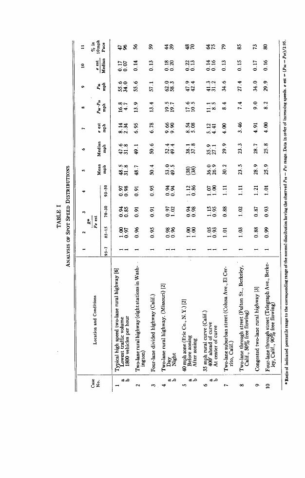
the pace.(These steps yield columns 5, 9 and 11 of table I.)

The percent of vehicles within the 10 mph pace is used as a measure of the dis-persion. Distributions with a high percentage of vehicles within the pace are pre-ferred. The percent within the pace may be determined easily from the array ofdata-no plotting of curves is necessary. The resulting figures are readily under-stood by laymen.

The 10 mph pace, however, is suited best to distributions of rural highwayspeeds. In urban areas, speeds are lower, and the 10 mph range usually covers toogreat a part of the curve.

Suggested Technique for Engineers-(a) Identify the 85th, 50th and 15th per-centile values from an array of the data (or from a graph of the cumulated per-centages). (b) Determine the 85th-15th percentile range.

The median (50th percentile) is as good a central measure as is the mean speed,and easier to obtain. For certain economic applications, the mean should be used,but for most purposes the median has at least as good theoretical justification.Actually, the difference between mean and median (in speed distributions) tendsto be very small indeed, as may be seen in table I, columns 5 and 6.

The range P85 - P15 is the actual speed in miles per hour, between the extremespeeds of the central 70% group. It is a measure easy to understand, and perhapseven more suitable than is the pace foi use in reports to the city council or the

~C. t-~'C 0%00

e' 00 0

- ~ .~j4Q~ U) If) ~ J4e't. 0 In0

o @ ._o -t -N C"I -bA oo 00 00 0 0C 0 0 0 0

o~~~~~~f If '.4) + u e) eu) (0°°9s def) (9 c 14 E

rw If ' - (9o00 t-( .-4 $ O . g. 0%g

ed \0~~ 0%0 _ -0 -00 00 t'- 0% 00 o£~~~ - cr '. o ' o ort- °4) °

1~0 $ CIfo or+) O0 '00 '0 0

:1 ^ oo o cf) 0% - '0%

eq 00~~~~~~~~~~~~~~

*b.o ' oo o oo00 0 .0 t oo cN )O0 ~ 0% 0 X90% 001- If)4-. 00 000 -

¢~~~~~~~~~~o 'o D m

U) - .0 *,.00 ¢~ '4k' 0V) 00% (9'1)40%

b 00~~.- 00 0 00%'00 ,) COf

-0 t--00 - I) a4 (9/0 . ---0

cn U''0%0 0 % 0% 0%% 0 -C 94/) 0%~ 00 0 0 0 00 ---0z 000'4~f 1.9 ~ 00 I)) 0 (9 00 If

0 n e*

CD 00 - 0

0

( z-'0,0 0'0 09 a,f - 4' 00 0%1Cl) ~~ ~ ~ ~ ~ ~ ~ ~ )

4 t~c-0 10 0o 00 - 0 -

rz

0~~~~~~~~~~.

0)

0 ~ ~~0)

0 ~ ~ ~~ ~ ~ ~ ~ ~ ~ ~~~0 0

- > o

-0 - ccDO-0) -~~~~~~~~ '- C$

o ~~~~~~6:: Mw~4, ~ ~ ~ ~ o -~~ 0) V 0'- 4

0 0~~~~~0 cc~~0) - -~~ ~~Z~b1) QO

0) 0) 0) 0ba d- b0

~~ 4 ~ ~ ~ -a~~~ ~~- cc4 c -0

*000 o00 -

SPEEDS AND TRAVEL TIMES 593

police department, or for release to the press. As a measure of dispersion it has theadvantage over the pace of suggesting immediately the total spread of the speeddistribution. It states explicitly the spread around the median of 70% of thespeeds, and may be expanded in usefulness by the following rule of thumb: 95% ofthe speeds lie within the median ± (P8s5 - P), (since P85 - P1 is roughly twicethe standard deviation oa; compare columns 7 and 8 of table I). It thus affords afair estimate of af for use in entering formulas for computing needed size of sample,etc.

The above technique gives a picture of the speed distribution sufficient for theusual engineering purposes. A more complete picture, lending itself to more carefulanalysis, is provided by the following proposed method.

6. Percentile method of analysisThe dispersion and skewness of speed distributions can be determined quickly

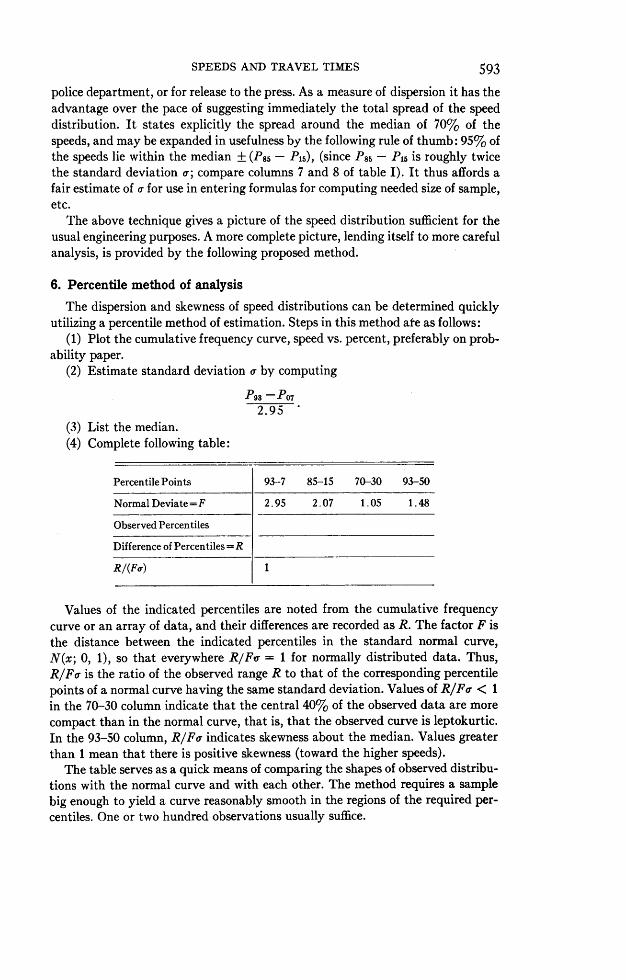
utilizing a percentile method of estimation. Steps in this method ate as follows:(1) Plot the cumulative frequency curve, speed vs. percent, preferably on prob-

ability paper.(2) Estimate standard deviation o- by computing

P93 -P072.95

(3) List the median.(4) Complete following table:

Percentile Points 93-7 85-15 70-30 93-50

Normal Deviate=F 2.95 2.07 1.05 1.48

Observed Percentiles

Difference of Percentiles = R

R/(Fa) 1

Values of the indicated percentiles are noted from the cumulative frequencycurve or an array of data, and their differences are recorded as R. The factor F isthe distance between the indicated percentiles in the standard normal curve,N(x; 0, 1), so that everywhere R/Fv = 1 for normally distributed data. Thus,R/Fo is the ratio of the observed range R to that of the corresponding percentilepoints of a normal curve having the same standard deviation. Values of R/Fa. < 1in the 70-30 column indicate that the central 40% of the observed data are morecompact than in the normal curve, that is, that the observed curve is leptokurtic.In the 93-50 column, R/Fa indicates skewness about the median. Values greaterthan 1 mean that there is positive skewness (toward the higher speeds).

The table serves as a quick means of comparing the shapes of observed distribu-tions with the normal curve and with each other. The method requires a samplebig enough to yield a curve reasonably smooth in the regions of the required per-centiles. One or two hundred observations usually suffice.


It will be observed that the method of estimating a, and the use of the median,cut computing labor almost to the vanishing point. (Raw data as frequentlygathered are already arrayed.)

The estimation of a as (P93 - P07)/2.95 has been discussed by Mosteller [5, p.3921 for samples of a normal population. It may often safely be used also for highlyabnormal distributions, if minimum error in the estimate is not essential. It iseasy to describe a distribution in which the error would be colossal, but it may beworth noting that for the rectangular, semicircular, and even right triangular dis-tribution, a lies between (P93 - P07)/2.95 and (P94- P6)/3.11. Perhaps, an ex-cellent all-around estimate is afforded by (P93.3 - Po6.7)/3.00.

The method of analysis uses (and describes) only that portion of an observeddistribution which lies between the 7th and the 93rd percentiles. For many engi-neering purposes, this central bulk of the data is of more importance than are thetails. In such cases, the above estimate of a- may be a more valuable measure ofdispersion than is the true standard deviation (and the median may be a bettercentral measure than is the mean). Another advantage in restricting the funda-mental percentile range lies in the fact that many available curves are smooth andwell defined within this range but become ragged beyond it. With the best tech-nique, to obtain an estimate of the 98th percentile requires a 50% larger samplethan is needed for an equally good estimate of the 93rd percentile (see Samplesize below).

7. Applications to preliminary data

Table I, columns 1 to 7, shows the application of the above method in the anal-ysis of spot speed distributions for several typical conditions on urban, suburban,and rural highways.

Values of R/Fa are generally close to 1 which suggests that the speed distribu-tions are roughly normal. This conclusion has been reached by Greenshields [31and is supported by the generally linear graph found on plotting on probabilitypaper, and by a reasonable value of P in applying the x2 test. There is a tendencyfor the distribution to be peaked in the center (column 3) and to display someskewness (column 4). These deviations from normality are not serious enough to

invalidate many applications of normal theory. For example, X + 1.037a (thenormal value of the 85th percentile) agreed with the observed 85th percentilewithin 0.lar (or about 0.6 mph) in 15 cases out of 16 examined.

Where speed is moderately limited by traffic volume, curves, or speed limits, thespot speed distribution remains roughly normal. The principal differences fromopen road conditions are of course lower average speed and smaller dispersion.There may be also a significant increase in concentration near the center, as incases lb and 6b. Columns 4 and 5 suggest that distributions of high mean speedare skewed toward the high speeds. (This tendency would probably be moremarked if more of the tail were included in column 4.)

Effect of Traffic Volume-The U.S. Bureau of Public Roads [6] reports that thereis a linear decrease of mean speed as traffic volume increases, when other conditionsare equal and the critical traffic density is not exceeded. Further analyses of theirdata reveal that the standard deviation a- of the speed distributions also decreases


approximately linearly, with increases in volume. The coefficient of variation o-/Xdecreases along a mild hyperbolic arc.When volume exceeds the practical road capacity, the speed distribution may

become so heavily skewed toward the higher speeds that all semblance of nor-mality is lost. Case 9 of table I is a good example.

Since traffic volume so materially affects speed distributions, it is apparent thatstudies of the effects of speed control measures should be made under comparablevolume conditions.

Other Factors-The effects of some other factors which influence speed distribu-tions have been the subjects of scattered studies, but not enough material appearsto have been published to justify important generalizations.

Posting of speed limits seems often to result in lower dispersion, with or withoutdecrease in average speed (see table I, case 5, and reference [9], but conflictingreports have been made [8, p. 6]). The effect of highway curves depends of courseupon the safe speed of the curve. If deceleration is required, dispersion should de-crease, but the coefficient of variation need not (table I, cases 6a, 6b, columns 7and 10). Posting of advisory speed signs at curves may substantially decrease thecoefficient ofvariation [7, p. 18].

8. Travel timeTravel times are usually obtained by utilizing test vehicles which "float" with

traffic, so as to simulate average traffic characteristics. Each driver is instructedto stay with traffic, and to pass as many cars as pass his vehicle. Travel times arealso obtained by taking data on all the vehicles composing a traffic stream. Inthis procedure, the license number of each vehicle and the times at which it entersand leaves a test section are recorded.

Relationships between travel times obtained by the two methods have been re-ported by Berry and Green [4].

Travel time studies furnish valuable data on the effectiveness of changed con-ditions, such as a new traffic signal system, one-way streets, rerouting of bus lines,changes in parking regulations, or widening or rebuilding of the street or highway.Travel time studies provide a quantitative measure of congestion and, in accord-ance with the test car procedure for obtaining the data, also furnish information onthe causes and the amounts of the delay. Results are also used in computing re-ductions in travel time arising from completed or proposed physical improvementsor changes in traffic controls.

The mean travel time is the value most commonly used in comparisons of thetravel time performance of a street or highway under the existing physical, traffic,and environmental conditions. It has the advantage of permitting direct computa-tion of total travel time for all traffic.

The median travel time, however, has its own advantage, since it correspondsto the median over-all speed whereas the mean travel time is not directly convert-ible to the mean over-all speed. Percentile ranges of travel times also are usefulas. a measure of dispersion, since they can be converted easily to over-all speedranges. Such ranges can be used in determining the timing for coordinated trafficsignal systems.


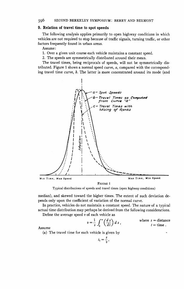
9. Relation of travel time to spot speedsThe following analysis applies primarily to open highway conditions in which

vehicles are not required to stop because of traffic signals, turning traffic, or otherfactors frequently found in urban areas.

Assume:1. Over a given unit course each vehicle maintains a constant speed.2. The speeds are symmetrically distributed around their mean.The travel times, being reciprocals of speeds, will not be symmetrically dis-

tributed. Figure 1 shows a normal speed curve, a, compared with the correspond-ing travel time curve, b. The latter is more concentrated around its mode (and

Iii a ~Spot Jeeo(sb- Travel Times as Computed'1Ij from Curve "'a"c- Travel Times with

Mixing of kRanks

,I IX '.

:1X \

Min Time, Max Speed Max Time, Min Speed

FIGURE 1

Typical distributions of speeds and travel times (open highway conditions)

median), and skewed toward the higher times. The extent of such deviation de-pends only upon the coefficient of variation of the normal curve.

In practice, vehicles do not maintain a constant speed. The nature of a typicalactual time distribution may perhaps be derived from the following considerations.

Define the average speed v of each vehicle as1 rS td sX d where s = distancev=!j8Qjs) ds,

Assume0 tdi t= time.

Assume(a) The travel time for each vehicle is given by

11= sV


(b) The spot speeds are normally distributed,(c) Vehicles maintain their respective ranks-that is, each remains at the same

distance (in a) from the spot mean at all points.Under these conditions, the average speeds v will be normally distributed, and

the time curve will be as shown in figure 1.(If, in two normal curves, points of the same a distances from the mean are

averaged together, the result will be a normal curve of average x and a. Thus anynumber of normal spot speed curves would compose into a normal over-all speedcurve, if ranks are maintained.)

Actually, the assumptions (a), (b) and (c) are all suspect. The problem is to esti-mate the influence of the errors each introduces.

Assumption (a) calculates the time as

fO (ds)whereas actually the time is given by

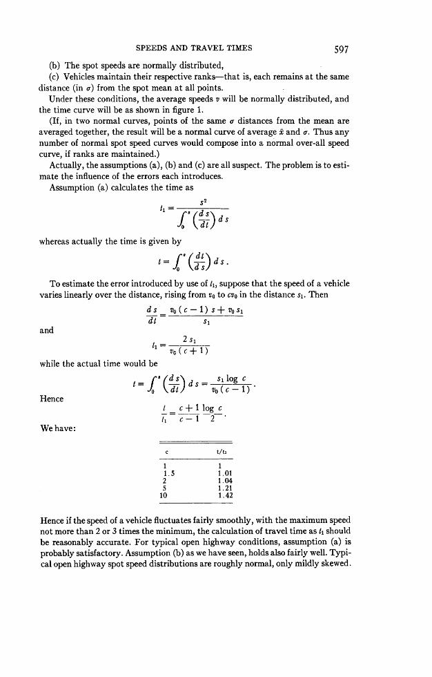
t= (d,tTo estimate the error introduced by use of ti, suppose that the speed of a vehicle

varies linearly over the distance, rising from vO to cvO in the distance s1. Then

d s vo (c-1)s+ vosidt S

and2 s1

(c + fT

while the actual time would be

t =if(ds) ds=- log_c

Hencet _ c +± log ctj c-1 2

We have:

c t/ti

1 11.5 1.012 1.045 1.2110 1.42

Hence if the speed of a vehicle fluctuates fairly smoothly, with the maximum speednot more than 2 or 3 times the minimum, the calculation of travel time as t, shouldbe reasonably accurate. For typical open highway conditions, assumption (a) isprobably satisfactory. Assumption (b) as we have seen, holds also fairly well. Typi-cal open highway spot speed distributions are roughly normal, only mildly skewed.


Assumption (c) is the poorest. Vehicles do not maintain their respective ranksat all points. Mixing of ranks has no effect on the mean value of the over-all speeds.It will however, reduce their standard deviation, since

( XlI+ X2)2 < (X-X1) 2+ (-X2)

If this mixing is symmetric around the over-all mean speed, the resulting over-allspeed distribution will remain symmetric (although it need not remain normal).

Practically, however, it is easier for slower vehicles to maintain their speed thanit is for the faster vehicles. More mixing of rank would be expected, with widerrank changes, on the high speed side of the mean.

Thus, under probable mixing conditions, the over-all speeds would have thesame mean as in the absence of rank mixing but would be compressed toward themean, and especially so on the high speed side. Their variance would be smaller,and skewness probably greater, and toward the low speeds.

The corresponding travel times would have smaller variance and probably muchgreater skewness toward the large times, than would times for the fixed rank con-dition.A comparison of distribution curves for the two conditions is shown schemati-

cally in figure 1. Curve b represents travel times arising from normal spot speeds(curve a) with ranks remaining fixed. Curve c is a typical travel time distributionunder rank mixing conditions, displaying smaller variance and greater positiveskewness.On streets having delays because of stops for traffic signals or other traffic con-

ditions it is difficult to relate travel times to spot speeds. The general effect of suchdelays on the travel time curve may be suggested by considering the probableover-all speed distribution. As delays increase, the average speed decreases, andthe speed distribution tends to become increasingly skewed toward the higherspeeds (table I, cases 7, 8, and 9). This offsets to some extent the tendency of traveltimes to be skewed toward the larger times, and in extreme cases may result in atravel time curve roughly symmetric about the median.

10. Applications to preliminary data

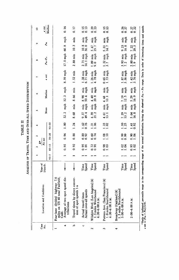
Table II shows applications of the same methods of analysis used in table I.Case 1 in table II shows comparisons of speeds and travel times for a four-lane di-vided rural highway. Case l-a represents the average of two "typical" spot speeddistributions. Case 1-b, the travel times by direct conversion of these average spotspeeds, is skewed toward the larger travel times. Case 1-c, showing the actual traveltimes for a 7.6 mile section, has greater skewness toward the large travel times, anda lower dispersion, as expected. Case 1-d shows that over-all speeds for this highspeed open highway are skewed toward the lower speeds, and have a lower disper-sion than the spot speed distribution in case 1-a.

Cases 2, 3, and 4 of table II show distributions of travel times and over-all speedsfor sections of heavily traveled streets controlled by traffic signals [4]. Case 2(Wilshire Boulevard) has a flexible progressive signal system with low delay. Driv-ers have more opportunities to select their own speeds, than in either case 3 or 4

b C COO >00 00 00 00 00C

i i -m To m_ bS ~~~0. E

x s E e~~EE3 E 3 EE = f

00 g m 00 C> *= 00 z

b tm e N Or me +NX~~~~CNO oo - -\0 _t 0~~~~~~~~~~~~-1 -O

> x s E fi as 0.

N~~~~~~~C 00 0~ ~~~00 Ro'WN e N@ V} Y = eC == vCz .== .< X . SS2,0 C~ V

z00 _O'-- m--

X N t o ~~~~~00oles a,ooocO 0

g¢ X O O~~~~~0 0- 00 O- --O-wO ~ ~~~ ~~~ I) C) Cs

cn 4),z <D ~'

W:Z; - N e + +-

6oo SECOND BERKELEY SYMPOSIUM: BERRY AND BELMONT

where delays and congestion are greater. On Potrero Avenue (case 3) there aretraffic signals at every block, and drivers have less chance to pick their own speed.Case 4 (Broadway) represents heavy traffic delay on a street with few traffic signals(5-6 P.M.), and also the same street during times of lighter traffic, with less delay(2-4 P.M.).

Case 4 (5-6 P.m.) with the heaviest congestion, shows the least skewness intravel time distribution (column 4). This is in accordance with the analysis givenabove. For cases of lesser delay, the travel times are markedly more skewed (andthe corresponding over all speeds far less skewed toward high speeds).

The range P85 - P15 of the over all speeds furnishes significant information ondispersion. The very low value for case 3 is caused by the characteristics of thesignal system, which here severely restrict speeds.

In comparing travel time distributions, P85 - P15 is directly useful only if thecourses being considered are of equal length. The ratio of the range to the medianaffords a more useful measure.

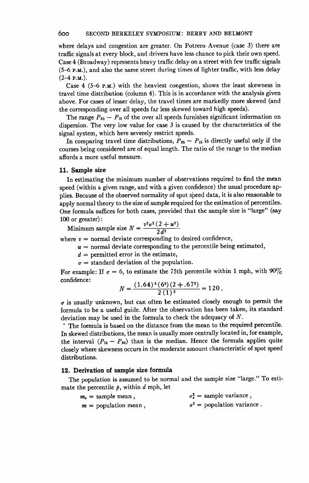
11. Sample sizeIn estimating the minimum number of observations required to find the mean

speed (within a given range, and with a given confidence) the usual procedure ap-plies. Because of the observed normality of spot speed data, it is also reasonable toapply normal theory to the size of sample required for the estimation of percentiles.One formula suffices for both cases, provided that the sample size is "large" (say100 or greater):Minimum sample size N = (2d+2)

where v = normal deviate corresponding to desired confidence,u = normal deviate corresponding to the percentile being estimated,d = permitted error in the estimate,a = standard deviation of the population.

For example: If a- = 6, to estimate the 75th percentile within 1 mph, with 90%confidence:

N = ((1.64) 2 (62) (2 +.6 72) -120.

a is usually unknown, but can often be estimated closely enough to permit theformula to be a useful guide. After the observation has been taken, its standarddeviation may be used in the formula to check the adequacy of N.

' The formula is based on the distance from the mean to the required percentile.In skewed distributions, the mean is usually more centrally located in, for example,the interval (P15- P85) than is the median. Hence the formula applies quiteclosely where skewness occurs in the moderate amount characteristic of spot speeddistributions.

12. Derivation of sample size formulaThe population is assumed to be normal and the sample size "large." To esti-

mate the percentile p, within d mph, let

m, = sample mean, au. = sample variance,m = population mean, a2 = population variance.

SPEEDS AND TRAVEL TIMES 6oi

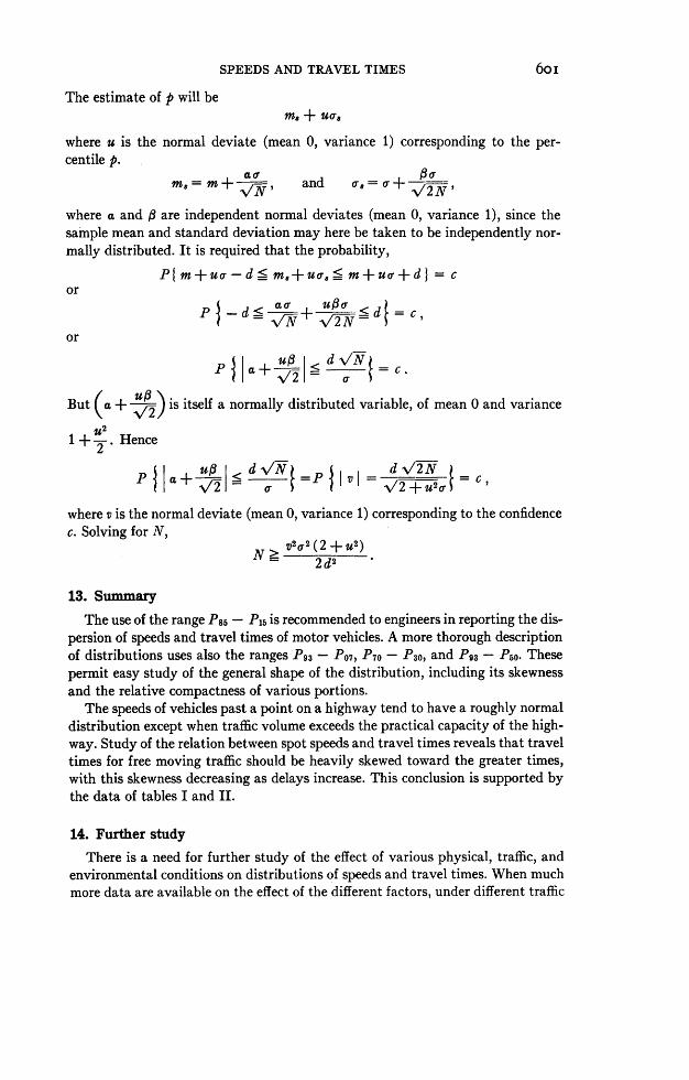
The estimate of p will bem. + uas

where u is the normal deviate (mean 0, variance 1) corresponding to the per-centile p.

mVN and O. = O + IN

where a and # are independent normal deviates (mean 0, variance 1), since thesample mean and standard deviation may here be taken to be independently nor-mally distributed. It is required that the probability,

Ptm+u r-d < m,,+uo,< m+uar+d = cor

d a o uf3cy<dP j- + -f t=cor

P I8 | a+ uO/ _ d -\/N =c

But (a + u# ) is itself a normally distributed variable, of mean 0 and variance

I +U2 . Hence

P | + u < dV/N=p dIvl x\N c

where v is the normal deviate (mean 0, variance 1) corresponding to the confidencec. Solving for N,

V2a2 (2+U2)N=2d2

13. SummaryThe use of the range P85- P5 is recommended to engineers in reporting the dis-

persion of speeds and travel times of motor vehicles. A more thorough descriptionof distributions uses also the ranges Pg3 - Po7, P70 - P3o, and P93 - Pr0. Thesepermit easy study of the general shape of the distribution, including its skewnessand the relative compactness of various portions.

The speeds of vehicles past a point on a highway tend to have a roughly normaldistribution except when traffic volume exceeds the practical capacity of the high-way. Study of the relation between spot speeds and travel times reveals that traveltimes for free moving traffic should be heavily skewed toward the greater times,with this skewness decreasing as delays increase. This conclusion is supported bythe data of tables I and II.

14. Further studyThere is a need for further study of the effect of various physical, traffic, and

environmental conditions on distributions of speeds and travel times. When muchmore data are available on the effect of the different factors, under different traffic


volume conditions, it may be possible to select standards for 85th-15th percentileranges which can be regarded as desirable in measuring the effectiveness of trafficcontrol programs.

The Committee on Speed Characteristics, of the Highway Research Board, inestablishing procedure for collection of data on speed characteristics, should con-sider the feasibility of covariance studies to isolate the effect of each importantvariable.

REFERENCES[1] Manual of Traffic Engineering Studies, Association of Casualty and Surety Executives, 1945,

pp. 20-23, 65-70.[2] Speed Regulation, National Safety Council, Chicago, 1941, pp. 53-56.[3] D. W. LOUTZENHEISER, "Percentile speeds on existing highway tangents" and discussion by

GREENSHIELDS, Proc. Hwy. Res. Bd., Vol. 20 (1940), pp. 372-392. Case 9 of table I is curve4-0 of p. 390.

[4] D. S. BERRY and F. H. GREEN, "Over-all speeds of motor vehicles in urban areas," Proc. Hwy.Res. Bd., Vol. 29 (1949), pp. 311-318.

[5] F. MOSTELLER, "On some useful 'inefficient' statistics," Annals of Math. Stat., Vol. 17 (1946),pp. 377-408.

[6] Highway Capacity Manual, Bureau of Public Roads, U.S. Government Printing Office, 1950,pp. 29-34.

[7] Report of Special Study on Speed Zoning, 1938 Report of Committee on Speed and Accidents,National Safety Council, 1938, pp. 1-47.

[8] C. C. WILEY, C. A. MATYAS, and J. C. HENBERGER, "Effect of speed limit signs on vehicularspeeds," mimeographed, Dept. Civil Engineering, University of Illinois (1949), pp. 1-19.

[9] D. S. BERRY, "Speed control," Proceedings, Convention Group Meetings, Amer. Assoc. of StateHwy. Officials, Vol. 34 (1948), pp. 361-365.

Documents

DISTRIBUTION OF VEHICLE SPEEDS AND TRAVEL TIMES