Vehicle value of travel time savings: evidence from a

Vehicle value of travel time savings: evidence from a group-based

modelling approach

Chinh Q. Ho1,*, Corinne Mulley1, Yoram Shiftan2,a, David A. Hensher1

1Institute of Transport and Logistic Studies (H73), The University of Sydney Business School, NSW 2006

Australia

2Faculty of Civil and Environmental Engineering, Technion-Israel Institute of Technology, Haifa 32000, Israel

a Visiting Professor to the Institute of Transport and Logistic Studies, The University of Sydney

*Corresponding author: [email protected]

[email protected]

[email protected]

[email protected]

Transportation Research Part A

Version: 28 January 2016

Abstract

The value of travel time savings (VTTS) accounts for a majority of the total user benefits in economic

appraisal of transport investments. This means that having an accurate estimate of VTTS for different

segments of travel continues to retain currency, despite there being a rich literature on estimates of

VTTS for different travel modes, travel purposes, income groups, life cycles, and distance bands. In

contrast, there is a dearth of research and evidence on vehicle VTTS, although joint travel by car is an

important segment of travel. This paper fills this gap by developing a group-based modelling

approach to quantify the vehicle VTTS and compares this with the VTTS for a driver with and without

a passenger. An online survey was conducted in Sydney in 2014 and the data used to obtain a

number of new empirical estimates of vehicle and driver VTTS. The new evidence questions the

validity of various assumptions adopted in current practice for valuing the time savings of car

passengers and multiple occupant cars.

Keywords: Vehicle VTTS, Driver VTTS, Passenger VTTS, Group models, Multiple occupant cars,

Economic appraisals.

1. Introduction

The value of travel time savings (VTTS) is one of the key components of user benefit for transport

projects. The theoretical basis for the treatment of time savings as an economic benefit is that

travellers are willing to pay a higher price for a quicker travel time. As VTTS accounts for a majority of

the total user benefits in economic appraisal of transport investments, typically from 60 to 80

percent of the total user benefit, it is crucial to have an accurate estimate of VTTS for different

mailto:[email protected]




2

segments of travel. As a result, a very large number of empirical studies on the estimation of VTTS

have been conducted in different countries. In some regions such as the UK, mainland Europe, North

America and Japan, the body of research is large enough for a meta-analysis to quantify the variation

of VTTS across travel segments (Abrantes and Wardman, 2011; Kato et al., 2010; Shires and de Jong,

2009; Zamparini and Reggiani, 2007). The different segments explored in empirical studies of VTTS,

and hence meta-analyses, are defined by travel mode (e.g., public transport vs. car), travel purpose

(e.g., commuting vs. business vs. other), group of travellers (e.g., high vs. low income), and distance

travelled (e.g., short vs. long journeys).

Joint travel by car constitutes an important segment of travel but the VTTS for car passengers and for

the entire group are rarely investigated (Ho, 2013; Ian Wallis Associates Ltd, 2014). Most studies of

car travellers’ VTTS have focused on the willingness to pay (WTP) of the car drivers. These studies

assume that the driver takes little or no account of passenger views when s/he makes a decision on,

for example, what route to take. Contrary to this assumption, it is in principle unknown whether the

driver behaves independently of other occupants, even if there are explicit instructions to that effect

in the experiment. For the purposes of economic evaluation and travel demand forecasting, a

decision is required as to how to obtain the VTTS for a vehicle. Different authorities may make

different decisions in this respect. For example, whilst the New Zealand Transport Agency’s Economic

Evaluation Manual (EEM) evaluates car passenger’s VTTS at 75 percent of the car driver’s values,

Austroads (Australian Road Transport and Traffic Agencies) and Transport for New South Wales

(TfNSW) use the same VTTS for car passengers and car drivers for transport demand models and

economic evaluations (Ian Wallis Associates Ltd, 2014; Austroad, 1997, TfNSW, 2013). Similarly, the

current practice in the Netherlands recommends 80 percent of the car driver VTTS for car passengers

(Significance et al., 2012, footnote 19, p. 72) while the most recent UK study on the VTTS

recommends that driver VTTS should be applied further to each occupant (ARUP et al., 2015, R10,

p.265). The difference in how VTTS is adjusted to account for car travel with multiple occupants

across national guidelines may be due largely to a lack of research and evidence on the vehicle VTTS

and/or the passenger’s VTTS relative to the driver values. Indeed, some research on the passenger’s

VTTS has been conducted in the UK, but the evidence is inconclusive and has led to a

recommendation of non-implementation in the absence of sufficient evidence to justify departure

from the status quo/current practice (Mackie et al., 2003, p.84; ARUP et al., 2015). This paper aims to

fill this challenging research gap using a new survey of car travel conducted in Sydney. In particular,

the paper explores the vehicle VTTS relative to the car drivers’ values and offers a method to derive

the vehicle VTTS for different group sizes.

Establishing VTTS for car passengers and group travel is very important for economic evaluation and

demand forecast of transport projects, especially those that involve travellers who trade travel costs

for travel times and opt for high occupancy vehicle lanes and toll roads. With very limited evidence

on the VTTS for car passengers and for group travel, economic evaluation and demand forecasts for

transport projects have to assume that the VTTS per car is the total of the driver’s value and the

passengers’ values (i.e., VTTS are additive for multiple-occupancy car). Whether this is a valid

assumption is open to question, and the answer to this research question has the potential to change

the outcome of investment appraisal. From an equity point of view, one could reason that for the

same income and travel purposes, car passengers would value travel time savings the same as car

drivers do, and thus applying the driver VTTS further to each occupant and summing up the VTTS to

3

obtain the vehicle VTTS, as in the current practice, is not too unreasonable. However, there are many

reasons why the additive assumption of VTTS for multiple occupancy vehicle may not be valid:

The decision of which route to take may be jointly made whereupon the VTTS obtained from

the group responses does not necessarily reflect the total VTTS obtained from separate

individual decision making. The only circumstances in which the group VTTS would be the total

of the individual VTTS would be cases like car-pooling where each member was able to choose

whether to join the group given specific time and cost information, and where the group

members were sensitive to time and cost (MVA et al., 1987). In all other cases, passengers and

drivers may still value their own travel time savings, but there is no market in which their

values, especially the passenger’s value, can be expressed fully, resulting in a vehicle VTTS

smaller than the summation of the driver and the passenger values.

The travel costs of the journey may be shared amongst the group members which will impact

on the willingness to pay for time savings expressed by the respondent. Insofar as the

respondent expresses his own preferences in terms of time savings, the VTTS obtained from

the respondent’s choices may then be interpreted as his own VTTS assuming contributions

from other occupants (MVA et al., 1987).

The driver might simply answer stated preference (SP) exercises or make revealed preference

(RP) choices solely on his own behalf, without consideration of other occupants’ preferences in

terms of time savings. The VTTS obtained should be then interpreted as the driver VTTS.

The driver might express a personal valuation of time savings for other occupants,

independent of their willingness to pay for saving travel time. The passengers VTTS as

perceived by the driver may be lower, the same, or higher than the value the passengers

themselves would express. Only when the driver perceived correctly how valuable the time

savings are to his passengers, does the vehicle VTTS obtained equal the total of the driver and

the passenger values.

Regardless of whether the driver takes account of the passenger preferences in terms of time

savings, the VTTS obtained from the driver responses to SP exercises or the driver choices in

the real market may reflect value of company. To the extent that travelling is more pleasurable

when company is provided, the driver VTTS will be reduced and insofar as the passengers were

a source of discomfort or stress, the driver VTTS will be increased (MVA et al., 1987; Hensher,

2008).

The driver faces the effort of driving whereas the passenger does not, which will impact on the

marginal disutility of time of drivers relative to passengers. Indeed, insofar as the passengers

can do worthwhile activities such as texting, checking emails or reading a book while travelling,

they may value time savings less than the driver does. Thus, applying the driver VTTS further to

each passenger for economic appraisal would be inappropriate.

The paper is organised as follows. The next section reviews the literature on the VTTS for car

passengers and car drivers of a multiple-occupant car. This is followed by a description of the car

travel survey designed to address the research question. A group-based modelling approach to

establishing the VTTS for the entire vehicle (i.e., the vehicle VTTS), the driver and the passenger is

suggested and model estimation results are then presented. The paper concludes with a discussion

of the main findings and suggestions for future research.

4

2. Literature review

A survey of the literature on the VTTS for car travel suggests that most studies have focused on car

drivers, with very few exceptions assessing the VTTS for car passengers or their influence on the

driver’s VTTS. Methodologically, these exceptions evaluate the VTTS for car passengers and group

travel using one of two approaches. The first approach treats the car passenger as an independent

decision-maker. The second approach assumes that the driver of the car is the main decision-maker

who may take into account the passenger’s VTTS in choosing, for example, the toll road in the

presence of a free road. This section examines the two approaches from the perspective of empirical

findings and underlying assumptions for the evaluation of vehicle VTTS.

Hensher (1986; 1989) took the first approach to evaluate the VTTS for car passengers. The car

passenger was treated as a separate mode for commuting in mode choice models from which VTTS

for all travel modes were derived. The results suggest that car passengers valued in-vehicle time

savings at about 75 percent of that of car drivers. This rate appears consistent with findings from

other studies of mode choice for non-commuting (Fosgerau et al., 2007), long distance travel (Román

et al., 2007) and the 1994 UK study that separately asked car drivers and car passengers their

willingness to pay for travel time savings (Accent and The Hague Consulting Group, 1999, p. 208-

213). Note that by asking car drivers and car passengers separately their willingness to pay/accept

with what are known as ‘transfer price questions’ the 1994 UK study assumes that car passengers are

independent decision-makers as in the case where car passenger is treated as a separate mode in a

mode choice model.

While the passenger’s VTTS relative to the driver’s values has been found to be consistent across

different studies and is adopted for economic appraisal in, for example, New Zealand (New Zealand

Transport Agency, 2013) and the Netherlands (Significance et al., 2012), the assumption underlying

the derivation of VTTS for car passengers is problematic for two reasons. Firstly, the passenger

preferences between alternatives in terms of time and cost variations are assumed to be

independent of the car driver preferences. There is little justification for this assumption and a

typical problem here relates to intra-household joint travel where a child comes along for the ride

and the parent decides what route/mode to take given the variations in time of cost between the

alternatives available to them. Secondly, using the passenger VTTS for implementation purposes

means that the VTTS for the vehicle varies substantially by its occupancy whilst in fact the marginal

cost of additional passengers (up to the vehicle capacity) is negligible. A more concerning problem

associated with the use of passenger VTTS alongside the driver VTTS is the assumption that these

values are additive. That is, if the driver VTTS is appraised at $10 per person hour and that of the

passenger is $8 per person hour, then the VTTS for the vehicle with two occupants (one driver and

one passenger) is valued at $10 + $8 = $18 per hour, and for the vehicle with three occupants this will

be $26 per hour. A behavioural violation of this additive assumption means that economic evaluation

methods may over-estimate the benefits of time savings from multiple occupant car users.

An exploratory analysis conducted by Ian Wallis Associates (2014) suggests that a violation of the

additive assumption of VTTS for multiple occupant cars is very likely, as the VTTS for two adults who

5

rideshare is not noticeably greater than the VTTS for the car driver alone. Although a caveat is

needed here since the evidence is based on a small and non-representative sample size (10

households known to the authors), this finding is in line with the results from other studies that

undertook the second approach to assess how the VTTS of a driver varies with occupancy. Before

discussing these studies in more detail, it is worth highlighting that the review by Ian Wallis

Associates identifies no studies of car passengers which have explicitly addressed the impacts of

personal characteristics (e.g., income, age) and preferences (e.g., doing worthwhile activities when

travelling) on the passenger VTTS.

Phase 3 of the MVA et al. (1987) work included two car stated preference (SP) surveys that assessed

the VTTS for group travel. One SP survey related to long distance car travel and the other focused on

route choice of motorists crossing the Tyne River by either the Tyne Tunnel (tolled) or the Tyne

Bridge (free). Both surveys asked car drivers to play a number of SP tasks and the study team offered

three possible ways of interpreting the VTTS obtained from the driver’s responses. The possible

interpretations are (i) the driver’s VTTS assuming passenger contributions, (ii) the vehicle VTTS

perceived by the driver, and (iii) the driver’s VTTS reflecting the value of company (see section 4.3.6,

p. 56). In terms of the empirical evidence, the long distance travel survey found that the VTTS

obtained from the car driver’s responses increased by about 40 percent with up to three passengers,

and increased by 65 percent when there were four or more passengers, compared to the VTTS of the

driver alone (or approximately an increase of 15 percent per passenger). By contrast, the Tyne

Tunnel crossing survey found that the obtained VTTS declined by 5 percent in the presence of a

passenger on commuting trips, but was unchanged for non-commuting trips (see section 8.4, p. 172).

In light of the conflicting evidence summarised above, the study team inclined to the results of the

long distance travel and suggested that the most likely interpretation of the obtained VTTS is the

vehicle VTTS as perceived by the driver. Also, the authors concluded that the VTTS of car passengers

was discounted by the driver who is typically making the choice. However, the extent to which the

VTTS of car passengers is discounted and the VTTS for car passengers relative to the driver’s values is

not clear as no surveys of car passengers were undertaken by MVA et al. (1987). This issue was

addressed in a subsequent work for the UK Department of Transport by Accent Marketing and

Research and the Hague Consulting Group (1999), which is referred to as the Accent and HCG study

hereafter.

The Accent and HCG study used an SP survey to examine the VTTS for car drivers and car passengers.

Each respondent was asked to play three games: two of which involved a trade-off between travel

time and travel cost (game 1: time-cost trade-off exercise, game 3: choice of tolled vs. free route),

and one randomly-assigned game involved a trade-off between travel time and one of the following

attributes: road characteristics (game2a: number of lanes, heavy vehicle access, and hard shoulder),

departure time (game 2b) and expected delay (game 2c). A sample of 4,000 car drivers and 400 car

passengers was obtained. With respect to the VTTS derived from time-cost trade-off exercise (game

1), the presence of a passenger was found to increase the VTTS obtained from the driver’s responses

by 9 percent for commuting trips and decrease the same VTTS by 15 percent for non-commuting

trips, but had no influence when travel was for business. By contrast, their analysis of the car

passenger surveys found that the VTTS for the car passengers was the same as for the car driver

value for commuting trips, about 11 percent less for non-commuting trips and 36 percent more for

6

business travel (p. 173). The conclusion was that drivers seem to take little account of the VTTS of

passengers when making their choices.

Hensher (2008) also used an SP survey to investigate the impact of car occupancy on the driver’s

VTTS for non-commuting travel in Sydney. Each respondent was asked to play 16 games which

involved a trade-off between travel times and travel costs among alternative routes. A sample of 222

interviews was obtained, giving 16 222 = 3,552 observations for model estimation. Using a mixed

logit model, Hensher found the average VTTS of the driver varied across the number of passengers

and decreased as the number of passengers increased. This result is consistent with Ramjerdi et al.

(1997) who found that the VTTS for a driver slightly reduced in the presence of one or two

passengers for non-commuting trips. However, the lower VTTS for the driver of multiple occupant

cars, as compared to the values for driver alone, runs entirely counter to the results of the Accent

and HCG study discussed above. Hensher acknowledged this difference and explained that “the

driver’s marginal disutility of travel time might be lessened in the presence of passengers who they

can chat to or even share some of the monetary costs” (p.69). If the car passengers share some of

the travel costs with the car driver, then the questions of interest are what is the VTTS of the car

passengers and how is the vehicle VTTS compared to that of the driver travelling alone? Hensher

(2008) acknowledges that his approach of treating the car driver as the main decision maker is not

able to establish the VTTS for passengers or a vehicle VTTS.

This brief review indicates that the international evidence on VTTS for passengers and drivers of

multiple occupant cars is very limited and inconclusive. In addition, all studies undertaken to date

have examined the vehicle VTTS based primarily on the driver’s responses to SP tasks. The only

exception is the Accent and HCG study which also included the passenger’s responses but their

responses were treated as independent from the driver’s responses. This may not be very realistic as

the preferences of the car driver could be different from preferences of his passengers, which when

occurs would force them to negotiate with each other to reach a consensus so that joint travel is

observed. Also, in the studies cited above, the SP experiments were designed to ask the respondent,

be it the driver or the passenger, to trade-off time and cost without specifying explicitly whether the

cost and time are those for the entire vehicle or those faced by the respondent himself. Leaving the

key variables of the SP tasks up to each respondent to interpret results in various ways of

interpreting the VTTS obtained, as discussed above under the MVA et al. work. In the current study,

we recognise that co-travellers (either the driver or passengers) may share travel costs (such as

parking, tolls or fuel costs) and allow the costs faced by each travel party to enter the SP tasks

explicitly. Whilst a unique interpretation of the VTTS derived from this kind of experiment is not

certain, advanced econometric models such as the one proposed below can be used to distinguish

the VTTS of the driver from that of the passenger and the vehicle. This is one area where the current

paper aims to contribute.

Another gap in the literature on the estimation of the vehicle VTTS is that all models to date are for

individual decisions with interactions between co-travellers being dealt with in an implicit manner.

That is, the respondent is assumed to take account of his co-traveller’s preference when responding

to SP tasks on the basis that the obtained VTTS is expected (and empirically shown) to be different

from the value for drive alone. However, the obtained value may not be the vehicle VTTS as there

7

exist different ways of interpreting the VTTS obtained (see MVA et al., 1987 and discussion above).

Dealing with inter-personal interactions in this way does not help us to distinguish the circumstances

in which co-traveller’s preference would be considered from the cases where this would be ignored.

This distinction, however, is necessary since the extent to which the preferences of other group

members are being considered has important implications on how the derived VTTS should be

interpreted. This paper attempts to tackle this area by examining the vehicle VTTS using a group-

based modelling approach which allows group members to interact, in terms of their utility function,

and choose the alternative that maximises the group utility. The empirical setting and modelling

approach are described in the next section.

3. Methodology

An individual weight modelling approach is proposed to capture the influence that each travel party

member may have on the joint decision. To this end, a customised survey was designed to collect

data for model estimation and the derivation of the VTTS for the vehicle as well as the car driver

(with and without passengers). The questionnaire is designed to obtain information on who pays for

the journey, which plays a critical role in deriving and interpreting the VTTS as well as designing SP

exercises that make sense to each respondent. Whether and to what extent the respondent takes

into account the preferences of other group members when making choices (the remaining bullet

points discussed in the introduction section) is taken care of by the modelling technique. This section

describes the survey instrument, the data and the modelling approach.

3.1 The survey

The centrepiece of the empirical study is a stated choice experiment designed to understand how the

preference, in terms of utility, of the co-travellers is taken into account by the respondent, be it the

car driver or the car passenger, when making a choice of route to travel for work/education,

business-related and non-work activities. The choice experiment consisted of three alternatives: the

current route and two unlabelled alternatives, called Route 1 and Route 2. Each route was described

by attributes representing the total travel cost the respondent pays, the total cost the co-travellers

pay, and the travel time for a round trip, defined and visually illustrated in the survey instrument as a

trip starting and ending at the same place with one or more destinations in between (also known as a

tour in the activity-based travel literature). All types of car user including driver alone, driver with

passenger(s), and passengers, were sought.

Two D-efficient designs were implemented for the experiment: one design for cases where travel

costs (including toll, parking and fuel costs) are split amongst co-travellers and the other for cases

where all costs are fully paid by one travel party member. The latter design was also applied for

respondents whose last round trip by car was as a driver only. Both designs were generated in such a

way that the total travel costs paid by the respondents and their co-travellers (if relevant) and the

round trip travel time for the current route were first acquired from respondents over the questions

related to their last round trip by car, while the attribute levels for the two unlabelled routes were

pivoted off of these values as minus or plus percentage shifts to represent a decrease or an increase

8

in travel time and travel costs incurred by each travel party member. The total travel cost paid by the

respondent and his co-travellers in their last car trip is computed using respondent’s answers to cost-

sharing questions. These questions ask each respondent the percentages that they contribute to

cover the fuel cost, toll cost and parking cost (if apply). With each component of the travel costs

being obtained prior to the SP experiment, we can compute the total travel cost paid by the

respondent and his co-travellers under the current route and pivot these to obtain values for the two

alternative routes. Table 1 shows the pivot levels for the two unlabelled alternatives in the cases

where the travel costs are split or not split across the group members.

Table 1. Pivot levels of the experimental designs with costs split and costs not split between

travellers

Attributes When costs are split When costs are not split

Total costs you pay ±5%, ±20%, ±40% 10%, ±20%, ±30%

Total costs other party members pay 0%, ±20% 10%, ±20%, ±30%

Travel time (round journey) 10%,±20% ±20%

Priors for the experimental designs were obtained from a pilot survey of 135 respondents spread

evenly across the 9 segments of car travel (3 purposes 3 types of car users). The experiments were

designed with conditions such that each choice made by the respondent required trade-offs between

travel time and travel cost for themselves or for their co-travellers. Specifically, one set of conditions

required that, if the current route costs more than Route 1 or Route 2, then the hypothetical routes

must take longer than the current route, and vice versa. This condition was applied for all possible

pairs of alternatives. Another set of conditions required that, if the total costs paid by the

respondents (i.e., attribute ‘total costs you pay’ in Table 1) on one route are higher than what they

have to pay on an alternative route, then the total costs incurred by their co-travellers (i.e., attribute

‘total costs other party members pay’) on this alternative route must not be lower, and vice versa.

This is to ensure that respondents always faced a trade-off between time and cost or between cost

paid by themselves and cost paid by their co-travellers. These designed conditions were tested with

NGene (Choice Metrics, 2012) using three groups of car use for short, medium and long travel, with

the reference levels selected for short travel [$2, $0, 30 mins] for medium travel [$6, $4, 60 mins],

and for long travel [$15, $10, 120 mins], with the first number in the brackets the cost paid by the

decision-maker, the second number the cost paid by co-travellers, and the last value the round trip

travel time.

The design for cases with no cost-sharing consisted of six choice tasks. The design for cases with cost

sharing amongst co-travellers consisted of 12 choice tasks which were blocked into two sets of six

choice tasks. One randomly selected block of the latter design was assigned to respondents if they

reported a sharing of costs on their last car trip. In both cases, each respondent was shown

sequentially six scenarios, each with three alternatives, and asked to select one route if they made

the same journey again. They were also asked to select one of the new routes in a subsequent

question where the current route is not available for choice. Figure 1 presents an illustrative choice

screen for cases where costs were split among the respondent and his co-travellers. The SP tasks for

9

cases where the travel costs were fully paid by one group member are similar to the one presented

in Figure 1, except that one of the two travel cost variables (costs you pay or costs other party

members pay) are set as zero for all routes.

Figure 1. Illustrative choice screen for cases where costs were split among group members

Apart from the information that was acquired for the design of the stated choice experiment, other

details were also collected. These included the main purpose of the respondent’s last round trip by

car, the way they travelled (as a driver only, as a passenger or as a driver with passengers), origin and

main destination of the round trip, the presence of any stop on the outward and return journeys,

auto body type, fuel consumption and year of manufacture of the vehicle used for the last round trip,

the number of people travelling together, the relationship between the travelling party, the

approximate distance all travel party members travelled together as well as age, income, travel

purpose (detailed classification), relationship to the driver (for all passengers), and licence status of

all travel party members. The respondents were also asked to indicate whether they had a joint bank

account or shared income with any co-travellers. After playing the games, respondents were asked to

describe themselves and their households, with questions relating to age, gender, access to car as a

driver, work status, occupation, household size and structure, number of cars owned by the

household, personal and household income.

10

The SSI panel (www.surveysampling.com) was used to obtain the sample and Sydney was chosen as

the study area where SSI has many thousands of participants. Ethics approval was obtained for the

experiment, and each respondent received a small incentive for a completed survey (be it cash,

points redeemable for a gift card or equivalent money that they can donate to a charity depending

on their preference). SSI panellists living in Sydney were randomly recruited from 14th March to 2nd

April 2014 via an email directing them to a customised online survey. In total, 2,061 invitation emails

were sent and a sample of 765 qualified respondents was obtained, resulting in a response rate of 37

percent. This is reasonably low compared to other online surveys we have previously undertaken

with SSI, and the reason for this was twofold. First, quotas were applied to screen out respondents

when the segments to which the respondents belong were full. Second, it was difficult to find

respondents in some segments of car use such as drivers with passenger(s) for business-related

travel. This screened out more respondents at the end of the survey period when some easy-finding-

respondent segments of the survey were closed while more difficult segments were still open for

recruitment.

3.2 The data

A process of cleaning and validating the data identified 46 respondents who reported inconsistent

trip details and 73 respondents whose last car tours were too short (less than 10 minutes) or too long

(longer than 5 hours). These respondents were removed from the analysis, reducing the sample to

645 usable respondents. Very short journeys were excluded as the difference between alternative

routes is too small to reveal the respondent’s VTTS (i.e., a 20 percent pivot off of a 10-minute journey

creates only a 2-minute difference in travel time between alternative routes). By contrast, very long

journeys were not included because of the potential of long distance travel contaminating the

dataset. Table 2 provides the summary statistics of the final sample, distinguishing drive alone and

shared ride respondents.

Table 2 shows a clear distinction in terms of socio and travel-related characteristics between the two

types of car users: driver alone vs. shared ride with the latter being split further by car occupancy of

2 or 3+ people. People driving alone appear to be older, have a higher personal income, pay standing

fees (e.g., registration fee, insurance and maintenance) more often, and have greater access to car

than those who shared ride (i.e., travel as a passenger or as a driver with passengers). In addition, on

average, people driving alone have a slightly shorter journey but incur a substantially higher cost ($5

for drive alone vs. $1.70 for shared ride by 2 persons or $3.36 for shared ride by 3+ persons). The

differences in travel cost between driving alone and shared ride users are likely to be due to

differences in travel purpose and the way in which travel costs are shared out among occupants.

With an average occupancy of 2.27 per vehicle ([2*299+3.36*75]/[75+299] = 2.27), on average

people who shared ride with others pay about 2.5 times less than those driving alone. The

distribution of travel purposes for driving alone compared to the shared ride subset is another

possible explanation for a large difference in travel cost. The shared ride sample includes more non-

work journeys but fewer business-related trips than the drive alone sample. As non-work travellers

have more opportunity than commuters and business travellers to avoid parking costs (by the

choices of destination and parking zones such as 2-hour free parking), the average travel cost per

person is lower for shared ride users than for people driving alone.

http://www.surveysampling.com/

11

Table 2. Summary statistics of the sample: drive alone vs. shared ride

Drive alone Shared ride by 2 Shared ride by 3+

Mean (s.d) Mean (s.d) Mean (s.d)

Main purpose is business-related (1/0) 0.27 () 0.10 () 0.09 ()

Main purpose is commute/education (1/0) 0.34 () 0.43 () 0.28 ()

Main purpose is non-work (1/0) 0.39 () 0.47 () 0.63 ()

Presence of stop on tour (1/0) 0.30 () 0.18 () 0.36 ()

Travel party size for most of the tour 1 (0) 2 (0) 3.36 (.56)

Travel time round trip 68 (52) 87 (52) 73 (61)

Total cost you pay round trip ($) 5.00 (7.26) 1.70 (5.08) 3.34 (8.40)

Respondent pays standing fee (1/0) 0.88 () 0.44 () .59 ()

Respondent age 47 (15) 44 (17) 39 (14)

Respondent is man (1/0) 0.41 () 0.42 () 0.31 ()

Number of household cars 1.77 (.96) 1.58 (.91) 1.57 (1.11)

Respondent income in $1000 57.60 (29) 45.80 (27) 43.20 (33)

Sample (number of respondents) 271 299 75

Note: () standard deviation is not meaningful for dummy variable.

It should be noted that the sample is not meant to be representative in terms of travel purpose, as

quotas were designed to obtain enough respondents in each travel segment for quantifying the

variation of VTTS across travel purposes and types of car users. Nevertheless, it was difficult to obtain

the quotas for business-related travel, especially in the shared ride segment, with the final sample

consisting of only 10 percent of the respondents (37 persons). The small sample of business-related

travel is the main reason for the exclusion of this travel segment from further analysis. Another

reason is that the choice experiment approach may not be able to reveal the VTTS for business

travellers when travel costs are paid by their employers (the analyst does not observe a trade-off

between time and cost from respondent’s choice of route when the payment is paid by the

employer).1

1 In this case, the Hensher approach (Batley, 2015) for valuing the VTTS for business travel is more suitable than

the approach employed in this study. Nevertheless, it is worth mentioning that even if the VTTS for business

travel is based on the Hensher approach, the influence of group travel might still be important as various terms

in the Hensher’s equation (i.e., VL and VW) are valued against the value of travel time savings, which if

appeared in this paper to be non-additive means that it would not be appropriate to sum individual Hensher

values to obtain the value for a group of people travelling for business-related purposes.

12

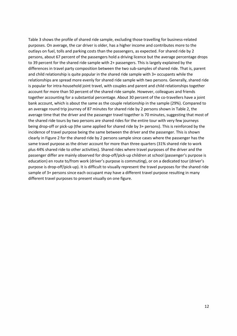
Table 3 shows the profile of shared ride sample, excluding those travelling for business-related

purposes. On average, the car driver is older, has a higher income and contributes more to the

outlays on fuel, tolls and parking costs than the passengers, as expected. For shared ride by 2

persons, about 67 percent of the passengers hold a driving licence but the average percentage drops

to 39 percent for the shared ride sample with 2+ passengers. This is largely explained by the

differences in travel party composition between the two sub-samples of shared ride. That is, parent

and child relationship is quite popular in the shared ride sample with 3+ occupants while the

relationships are spread more evenly for shared ride sample with two persons. Generally, shared ride

is popular for intra-household joint travel, with couples and parent and child relationships together

account for more than 50 percent of the shared ride sample. However, colleagues and friends

together accounting for a substantial percentage. About 30 percent of the co-travellers have a joint

bank account, which is about the same as the couple relationship in the sample (29%). Compared to

an average round trip journey of 87 minutes for shared ride by 2 persons shown in Table 2, the

average time that the driver and the passenger travel together is 70 minutes, suggesting that most of

the shared ride tours by two persons are shared rides for the entire tour with very few journeys

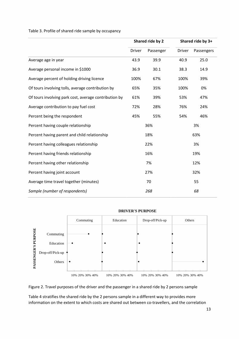
being drop-off or pick-up (the same applied for shared ride by 3+ persons). This is reinforced by the

incidence of travel purpose being the same between the driver and the passenger. This is shown

clearly in Figure 2 for the shared ride by 2 persons sample since cases where the passenger has the

same travel purpose as the driver account for more than three quarters (31% shared ride to work

plus 44% shared ride to other activities). Shared rides where travel purposes of the driver and the

passenger differ are mainly observed for drop-off/pick-up children at school (passenger’s purpose is

education) en route to/from work (driver’s purpose is commuting), or on a dedicated tour (driver’s

purpose is drop-off/pick-up). It is difficult to visually represent the travel purposes for the shared ride

sample of 3+ persons since each occupant may have a different travel purpose resulting in many

different travel purposes to present visually on one figure.

13

Table 3. Profile of shared ride sample by occupancy

Shared ride by 2 Shared ride by 3+

Driver Passenger Driver Passengers

Average age in year 43.9 39.9 40.9 25.0

Average personal income in $1000 36.9 30.1 38.3 14.9

Average percent of holding driving licence 100% 67% 100% 39%

Of tours involving tolls, average contribution by 65% 35% 100% 0%

Of tours involving park cost, average contribution by 61% 39% 53% 47%

Average contribution to pay fuel cost 72% 28% 76% 24%

Percent being the respondent 45% 55% 54% 46%

Percent having couple relationship 36% 3%

Percent having parent and child relationship 18% 63%

Percent having colleagues relationship 22% 3%

Percent having friends relationship 16% 19%

Percent having other relationship 7% 12%

Percent having joint account 27% 32%

Average time travel together (minutes) 70 55

Sample (number of respondents) 268 68

Figure 2. Travel purposes of the driver and the passenger in a shared ride by 2 persons sample

Table 4 stratifies the shared ride by the 2 persons sample in a different way to provides more

information on the extent to which costs are shared out between co-travellers, and the correlation

Others

Drop-off/Pick-up

Education

Commuting

Commuting Education Drop-off/Pick-up Others

10% 20% 30% 40% 10% 20% 30% 40% 10% 20% 30% 40% 10% 20% 30% 40%

Travel purposes of driver and pasenger in a shared ride by 2 persons

PA

SS

EN

GE

R'S

PU

RP

OS

E

DRIVER'S PURPOSE

14

between cost-sharing and other characteristics of the journey. As indicated by the sample size, the

incidence that travel costs were shared out between group members is quite small (34/268 = 13%).

Of these cases, the average contribution of driver and passenger is close to 50 – 50 percent. A deeper

investigation into the cost-sharing sample suggests that the most popular cost that was shared

between travel party members was the fuel cost. More specifically, about three in four respondents

stated that they contribute 50 percent to cover the fuel cost. This is likely to be paid out of a joint

account, which has a much higher incidence (21/34) under cost-sharing travel (i.e., respondent pays

something but not all of the travel costs) than under costs being paid fully by one person (i.e.,

respondent pays all or nothing). There is, however, not much difference between cost-sharing and

cost-not-sharing in terms of time people travel together and the incidence that the group members

have the same travel purpose (67% under cost-not-sharing vs. 74% under cost-sharing).

Table 4. Sample profile of shared ride by 2 persons, segmented by respondent’s contribution to costs

Respondent's contribution to cost

All (100%) Something Nothing (0%)

Number of drivers (ave. contribution if pay something) 50 18 (51%) 52

Number of passengers (ave. contribution if pay something) 8 16 (49%) 124

Number of cases having same travel purpose 42 25 115

Number of cases having a joint account 24 21 28

Average age in year 54 55 39

Average annual income in $1,000 49 38 46

Average time travel together (minutes) 47 63 79

Average round trip time (minutes) 61 71 95

Sample size (number of respondents) 58 34 176

3.3 The model

To capture the influence that each group member has on the choice of route under a shared ride, a

joint decision model incorporating decision maker importance weights is developed. Under this

model, decision-makers (i.e., the respondents) are assumed to maximise the group utility as opposed

to their own utility when choosing a route for shared ride. The utility that a group of g individuals

(i.e., co-travellers) derives from a route r is defined as the weighted sum of group member’s utility,

and is given in equations (1) and (2).

1

g

gr i ir gr

i

U V

(1)

15

1

1 and 0,g

i i

i

i

(2)

Vir is the observable utility that a group member i derives from an alternative r, εgr is the unobserved

utility associated with group g and route r, and i are the importance weights that effectively re-scale

the utility of a group member i relative to other group members’ utilities. To be consistent with

McFadden’s (1978, p.80) principles of stochastic utility maximisation, it is necessary that the

importance weights sum to one as specified in equation (2). More specifically, this condition ensures

that the underlying utility generating function is homogenous of degree one (see Appendix for

proof). In addition, as i represents the importance weight of member i in the group decision, it is

also required that i 0, i. The conditions specified in equation (2) provide the generating function,

not only a necessary property to be consistent with utility maximisation but also a useful

interpretation in which a group member may not participate in the joint decision (i = 0) while all

participants’ importance weights sum to one.

The importance weights i can be parameterised to be a function of personal income, travel

purpose, and other factors such as driving licence status, gender and age (collectively denoted as Zi).

This is to recognise the scope for systematic heterogeneity in the importance weights, in line with

O’Neill and Hess (2014) and Dosman and Adamowicz (2006). To ensure that the conditions (2) are

met, the importance weights are formulated as a logit model (3) in which importance weights are

bounded between zero and one, and sum to one.

1

exp( )

exp( )

ii g

j

j

Z

Z

(3)

With this specification, the group-based decision model, represented by equations (13), allows the

influence of each member on the group decision to be context dependent. That is, the model allows

different members of a group to have different influences on a group decision, dependent on the

individual’s preference intensity, experience and personal characteristics. Given that potential

factors influencing the importance weights are endogenously estimated, this makes the current

study different from the above cited studies in which heterogeneity in the importance weight is

treated as random (O’Neill and Hess, 2014) or externally estimated (Dosman and Adamowicz, 2006).

In estimating the model, the estimator will identify the importance weights (to be exact, the

parameters associated with proxy variables for the importance weights) to maximise group utility.

This modelling structure lends itself to the familiar logit form. The general form of the model departs

from a standard specification of linear-in-parameters for the observable utility, .ir i irV X In the

current context of a route choice experiment, Vir is specified as a function of the travel time and

travel cost that the group member i spends on an alternative route r:

16

ir i i r timei ir costi irV X Time Cost (4)

Note that individual-specific parameters are used for time and cost to capture the heterogeneity in

sensitivities across group members. This is equivalent to a specification where the weights vary

across attributes, with each attribute being accompanied by a generic parameter (see for example

O’Neill and Hess, 2014). Assuming an iid type I extreme value distribution for the random terms εgr,

the probability that group g choose an alternative route r in a choice situation of R routes can be

expressed as equation (5).

1

1 1

exp( )

exp( )

g

i i r

igr gR

i i r

r i

V

P

V

(5)

Preference heterogeneity may be layered on top of the group-based model (5) in the form of random

parameters (6) or error components (7) or both.

ik k k ik

(6)

gr gr r grE (7)

k is the population mean of the individual parameter ik associated with attribute k, ik is the

individual specific heterogeneity with mean zero and standard deviation one, k is the standard

deviation of the distribution of ik around k , grE are error components which are alternative

specific with zero mean and standard deviation one, r is the standard deviation parameter, and gr

is iid extreme value.

The full model with all components is:

1

1 1

exp ( )

exp ( )

g

i i i r r gr

i

gr gR

i i i r r gr

r i

X E

P

X E

(8)

The group-based model (8) is applicable for any group size through an appropriate specification of

the importance weight function. With multiple occupancy vehicles, the passengers are distinguished

by their travel purposes, income levels, ages and other personal characteristics that go into vector Zi

in eq. (3). The importance weight of each group member can then be estimated given that time and

cost each group member spends on an alternative route are known. The proposed model can also be

17

extended to reflect both group decision and individual decision. This is done by modifying the utility

function (1) as:

1

(1 )g

r i ir ir r

i

U d V d V

(9)

where d is a dummy variable equal to one under joint travel and zero otherwise.

4. Estimation results

This section presents the empirical model results for both joint and individual travel by car. As noted

in section 3.3, the model is able to reflect both individual and group decisions with multiple decision-

makers. However, the empirical data consist of a small sample of shared ride by 3+ people, spreading

across different levels of car occupancy (46 observations with three occupants, 19 observations with

four occupants, and 3 observations with five occupants), but mainly covering shared rides to a joint

social/recreation activity. Including these observations in the model specification results in a singular

variance-covariance matrix (i.e., the model could not be estimated). The estimation has therefore

been restricted to the choice of drive alone and shared ride by two persons only.

Different specifications for the presence of preference heterogeneity (equations 6 and 7) were

explored using Nlogit pre-released version 6 (April 2015). No statistical evidence was found to

support the presence of preference heterogeneity in the marginal utilities of the group after

numerous distributional assumptions for the group utility parameters and the error component

model have been tried. There is, however, heterogeneity in the importance weight parameters and

this heterogeneity is mostly deterministic and linked to personal income, travel purpose and the role

of the travellers when shared ride (more on this later). Regarding the model for drive alone, the

random parameters associated with travel time and travel cost are statistically significant. Thus, the

finally adopted model has a non-linear MNL form (due to the presence of the importance weight

parameters i which multiply with time and cost parameters) for the shared ride sample and a mixed

logit form for drive alone with all random parameters assumed to follow a constrained triangular

distribution. A number of distributions including normal, log-normal and constrained triangular were

explored for the random parameters, and the best statistical fit was the constrained triangular

distribution where the spread (equal half the range and the standard deviation times √6) is

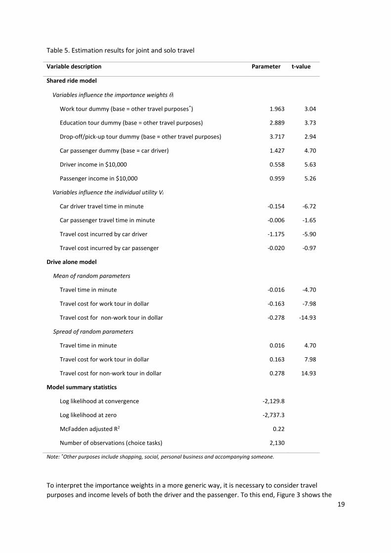
constrained to equal the mean. Table 5 shows the estimation results.

All the parameter estimates have the expected sign and the combined model fits the data reasonably

well with the McFadden adjusted R2 of 0.22. Table 5 shows that the importance weight an individual

possesses, relative to their co-traveller’s importance weight, is significantly influenced by the travel

purposes and incomes of both travellers. The relative magnitudes of the parameters associated with

the travel purpose are interesting with drop-off/pick-up passengers having the largest parameter

(3.717), followed by education (2.889) and work tours (1.963). It should be noted that if both driver

and passenger have the same travel purpose, then the purpose has no impact on importance

weights. For these cases, the importance weights are determined by other variables including income

levels of both driver and passenger as well as the dummy variable that distinguishes passenger from

18

driver. The travel purposes that the driver and the passenger usually ‘shared’ on a shared ride tour

include commuting, education and others (the base) while drop-off/pick-up relates exclusively to the

driver (see Figure 2). This makes the interpretation of an individual parameter impossible as the

usual ‘ceteris paribus’ assumption does not hold for two reasons. The first reason, applied to a

majority of the sample, relates to income levels with the driver having a higher income than the

passenger (on average, the car driver’s income is 20 percent higher than that of the car passenger,

see Table 3). The second reason concerns a smaller number of observations where the driver and the

passenger have different travel purposes (see Figure 2). The only parameter of the importance

weight functions that can be interpreted individually is the car passenger dummy (identify the

passenger from the driver), but this requires other variables (i.e., travel purpose and income) to be

the same between the driver and the passenger (i.e., the ceteris paribus assumption). In these cases,

the utility of the car passenger is weighted more heavily than the driver’s utility, although the

contribution of the passenger utility to the group utility is quite small, given the insignificance of

passenger cost parameter. The significance of passenger dummy appears to have little relevance to

the passenger’s contribution to pay for travel costs since an inclusion of a dummy variable identifying

who is paying (passenger vs. driver) and other related variables such as the existence of a joint

account does not change the significance of the passenger dummy parameter. This is based on a

small sample of passengers who actually contribute to pay for travel cost. In a sample with a larger

number of passengers incurring some cost, who is paying may have an influence on the choice. It is

worth mentioning that variables identifying the respondent were also included in the importance

weight, as a main effect and/or interaction effects, but none of these were found to be statistically

significant. This lends support to our assumption that respondents maximise the group utility rather

their own utility, which otherwise would result in a significant parameter for at least one of these

variables (suggesting that respondents give greater weight to themselves than to other occupant).

19

Table 5. Estimation results for joint and solo travel

Note: *Other purposes include shopping, social, personal business and accompanying someone.

To interpret the importance weights in a more generic way, it is necessary to consider travel

purposes and income levels of both the driver and the passenger. To this end, Figure 3 shows the

Variable description Parameter t-value

Shared ride model

Variables influence the importance weights i

Work tour dummy (base = other travel purposes*) 1.963 3.04

Education tour dummy (base = other travel purposes) 2.889 3.73

Drop-off/pick-up tour dummy (base = other travel purposes) 3.717 2.94

Car passenger dummy (base = car driver) 1.427 4.70

Driver income in $10,000 0.558 5.63

Passenger income in $10,000 0.959 5.26

Variables influence the individual utility Vi

Car driver travel time in minute -0.154 -6.72

Car passenger travel time in minute -0.006 -1.65

Travel cost incurred by car driver -1.175 -5.90

Travel cost incurred by car passenger -0.020 -0.97

Drive alone model

Mean of random parameters

Travel time in minute -0.016 -4.70

Travel cost for work tour in dollar -0.163 -7.98

Travel cost for non-work tour in dollar -0.278 -14.93

Spread of random parameters

Travel time in minute 0.016 4.70

Travel cost for work tour in dollar 0.163 7.98

Travel cost for non-work tour in dollar 0.278 14.93

Model summary statistics

Log likelihood at convergence -2,129.8

Log likelihood at zero -2,737.3

McFadden adjusted R2 0.22

Number of observations (choice tasks) 2,130

20

kernel distribution of importance weights in the sample. To produce the kernel distribution shown,

the parameters associated with the variables that influence the importance weights are multiplied by

the values of the variables, and equation (3) is applied to compute the importance weight for each

individual in the sample from which the kernel distribution is estimated. It can be seen from Figure 3

that the disutility of the car passenger is weighted more heavily than that of the car driver, with an

average weight held by the passenger of 0.777, while the average weight of the driver was 0.223.

There were very few cases where one travel party member, be it the driver or the passenger,

dominated the choice. The evidence challenges the two approaches used in the literature in which

the car passenger is treated as an independent decision-maker or the car driver is considered as the

main decision-maker (see section 2).

Figure 3. Sample distribution of importance weight held by car driver (thetad) and car passenger

(thetap)

Turning to the utility of travel party members, Table 5 shows that parameters associated with travel

time and travel cost incurred by the driver are highly significant, but the parameters for the

passenger are not statistically significant at the 95 percent level of confidence. While the parameter

associated with the passenger time has a 90 percent level of confidence, the level of confidence is

much lower (67%) for the parameter associated with the passenger cost. This is presumably due to

the small sample of passengers who actually contributed to pay for the travel costs incurred in a joint

tour (see Table 3). With respect to solo travel (i.e., drive alone), both means and spreads of the

random parameters associated with travel time and travel costs are highly significant, suggesting the

presence of heterogeneity in the sample preference for travel time and travel cost. The effect of

travel purpose on individual’s sensitivity to travel costs is included by interaction terms between

travel cost and travel purpose. The interaction parameters are statistically different from each other,

with solo commuters (DA_WORK) being found to be less sensitive to travel cost than solo drivers

travelling for other purposes (DA_OTHER), as expected.

Kernel Density Estimates

.72

1.44

2.17

2.89

3.61

.00

.20 .40 .60 .80 1.00.00

THETAD THETAP

Density

21

The VTTS for the vehicle and for the driver (travel alone or travel with a passenger) can be derived

from the time and cost parameters. The passenger VTTS can be calculated as well but it would not be

reliable, given the statistical non-significance of the corresponding parameters, especially the cost

parameter. Figure 4 compares the vehicle VTTS (labelled VEHICLE in Figure 4) with that of the drivers

who travel with one passenger (DRIVER) and drivers who drive alone, with the latter distinguishing

work (DA_WORK) and non-work (DA_OTHER) travel. It should be noted that the distribution of the

vehicle and the driver VTTS is obtained from the variation in importance weight across the sample

while the distribution of VTTS for drivers without a passenger (DA_WORK and DA_OTHER) is derived

from the random parameters associated with time and cost. These are very different types of effect:

one results from the weight that each occupant carries into the group choice and one results from

the variation in driver’s sensitivity to travel time and cost. The average VTTS for the driver with one

passenger is $13.65 per hour (standard deviation of $8.15 per hour) which is higher than the average

VTTS for the driver without a passenger ($8.30 per hour if drive alone to work and $5.40 per hour if

drive alone to non-work). These VTTS are in line with the values estimated for non-work travel and

for the car driver with one passenger in Sydney (Ho and Mulley, 2013; Hensher, 2008), and in

Australia in general (Litman, 2011; Australian Transport Council, 2006).

Figure 4. Distribution of vehicle vs. driver VTTS ($/hour)

Figure 4 also shows the distribution of VTTS for vehicle with two occupants. To establish the vehicle

VTTS, the marginal cost of the group (or the entire car) is calculated as the weighted average of the

marginal utility of total travel cost where the weights are the costs incurred by the driver and the

passenger. Given that the time is the same for driver and passenger when they travel together, the

vehicle VTTS formula is expressed as follows:

Vehicle vs. Driver VTTS (dollars/hour)

.031

.062

.093

.124

.155

.000

10 20 30 40 500

VEHICLE DRIVER DA_WORK DA_OTHER

Density

22

cos cos

cos

60time time

d d p ptimecar t t

d d d p p pt

d p

MUVTTS

Cost CostMU

Cost Cost

(10)

where Costd and Costp are the total costs incurred by the driver and the passenger on the chosen

route in each choice task; d and p are individual power weight calculated using equation (3) with a

reference to the annual incomes and travel purposes of the driver and the passenger in their last

round trip journey by car; and cos cos, , ,time time t t

d p d p are the parameters associated with time and

cost of the driver and the passenger as shown in Table 5. The average VTTS for vehicle with two

occupants is $17.80 per hour with a standard deviation of $9.70 per hour. The vehicle VTTS is about

30 percent higher than the driver VTTS. However, this does not mean that the passenger VTTS is 30

percent of the driver VTTS as the driver’s and the passenger’s VTTSs are not additive but are

weighted by the importance weights to form a group VTTS. Only when each co-traveller holds an

equal weight to the joint decision and when all of them are equally sensitive to travel time and travel

cost does the additive assumption of VTTS for the car driver and for the car passenger hold. Clearly,

this is not the case with this empirical dataset where the passengers appear to possess a larger

weight and have different preferences to time and cost than the driver.

5. Model application

Given that the sample used for parameter estimation is not representative of the population, it is

necessary to apply the model to the population data in order to derive the vehicle VTTS for transport

project appraisal. To this end, a joint household travel dataset constructed from the Sydney

Household Travel Survey (HTS) is used (see Ho, 2013; Ho and Mulley, 2013 for a full description of

how to construct such the dataset from the HTS). The parameters shown in Table 5 are then applied

to compute the importance weights possessed by the car driver and the passenger, depending on

their travel purpose and personal income, both available in the Sydney HTS. Figure 5 shows the

population distribution of the importance weights held by the driver and the passenger of shared

ride tours by two household members. Given that shared rides involving only household members

(called intra-household shared ride) account for more than 85 percent of total shared rides (Vovsha

et al., 2003), the importance weights derived from the intra-household joint dataset should closely

approximate the importance weights for a general shared ride sample (i.e., regardless of the

occupants are from the same or different households). Figure 5 shows that the population

distribution of the importance weights is quite different from the sample distribution shown in Figure

3 highlighting the need to apply the model to the population data for the estimation of the vehicle

VTTS. On average, car drivers do possess a higher weight (0.55) than the car passengers (0.45), in

contrast to the discussion of results earlier in the paper which is based on the sample data.

23

Figure 5. Population distribution of importance weight held by the driver (thetad) and the passenger

(thetap)

In addition, the estimation of the vehicle VTTS requires the relative contribution of the passenger

and the driver to cover the travel costs. While the travel costs of a tour can be derived from the

Sydney HTS, the contribution from the driver and the passenger is unknown. Thus, the average

sample ratio of passenger costs to driver costs (0.33:0.67) is assumed for the population. With these

assumptions, the average vehicle VTTS with two occupants (vehicle VTTS) is estimated at $13.50 per

hour, with a standard deviation of $7 per hour. The corresponding value for the driver with one

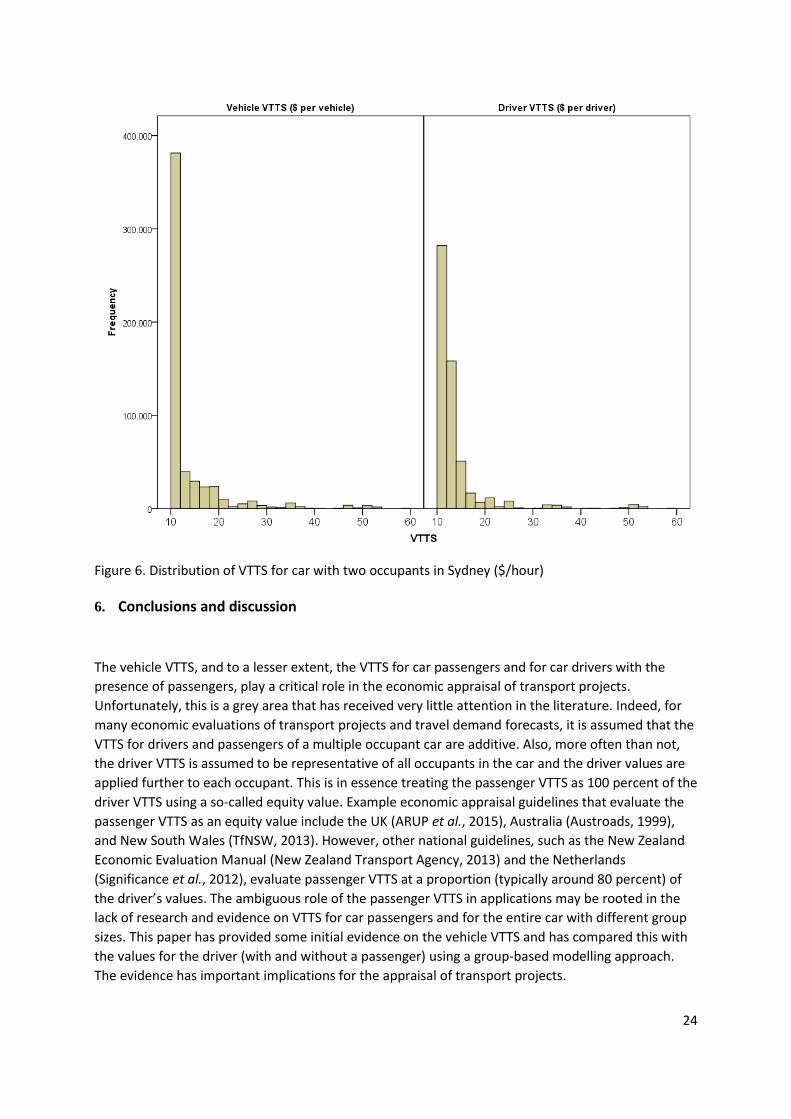
passenger is estimated at $12.00 per hour (standard deviation of $6). Figure 6 shows a histogram of

VTTS for the vehicle and the driver with one passenger, accounting for the importance weights

assigned to each occupant.

Kernel Density Estimates

.39

.78

1.17

1.55

1.94

.00

.20 .40 .60 .80 1.00.00

THETAD THETAP

Density

24

Figure 6. Distribution of VTTS for car with two occupants in Sydney ($/hour)

6. Conclusions and discussion

The vehicle VTTS, and to a lesser extent, the VTTS for car passengers and for car drivers with the

presence of passengers, play a critical role in the economic appraisal of transport projects.

Unfortunately, this is a grey area that has received very little attention in the literature. Indeed, for

many economic evaluations of transport projects and travel demand forecasts, it is assumed that the

VTTS for drivers and passengers of a multiple occupant car are additive. Also, more often than not,

the driver VTTS is assumed to be representative of all occupants in the car and the driver values are

applied further to each occupant. This is in essence treating the passenger VTTS as 100 percent of the

driver VTTS using a so-called equity value. Example economic appraisal guidelines that evaluate the

passenger VTTS as an equity value include the UK (ARUP et al., 2015), Australia (Austroads, 1999),

and New South Wales (TfNSW, 2013). However, other national guidelines, such as the New Zealand

Economic Evaluation Manual (New Zealand Transport Agency, 2013) and the Netherlands

(Significance et al., 2012), evaluate passenger VTTS at a proportion (typically around 80 percent) of

the driver’s values. The ambiguous role of the passenger VTTS in applications may be rooted in the

lack of research and evidence on VTTS for car passengers and for the entire car with different group

sizes. This paper has provided some initial evidence on the vehicle VTTS and has compared this with

the values for the driver (with and without a passenger) using a group-based modelling approach.

The evidence has important implications for the appraisal of transport projects.

25

The evidence herein that car passengers hold just slightly less weight (0.45) than car drivers (0.55) on

the choice of route for shared ride questions the validity of the assumption that the car driver is the

main decision-maker. From an empirical perspective, the evidence challenges the practice of

approximating the passenger VTTS at a proportion of the driver VTTS or ignoring the passenger VTTS

entirely for economic evaluation and travel demand forecasting. In addition, the VTTS of the driver

and the passenger are found to be non-additive in this study, with the vehicle VTTS being not much

higher than the driver VTTS. Although this study was unable to establish a reliable estimate of a

passenger VTTS due to a small number of observations, this result suggests that a vehicle VTTS

should be used instead of adding the passenger VTTS to the driver VTTS. This would at least remove

the risk of double counting the benefit from high occupancy vehicle users where the magnitude of

the risk depends on the extent to which the assumption on the additivity of VTTS is violated.

Given the VTTS estimated in this paper, the practical question of interest relates to the VTTS that

should be used for multiple occupancy vehicles in transport project appraisal and how this value

compares to the one under current practice. Table 6 summarises the VTTS currently used in Australia

and New Zealand (NZ) for economic appraisal and compares these with the values derived from the

current study. Australian, NZ, and TfNSW values are chosen for comparison since the current study is

undertaken in Sydney, NSW. The emphasis here is on the relativities of the VTTS for drive alone, car

passenger and the vehicle. On the one hand, the current NZ practice evaluates the driver VTTS at

$7.80 per hour for commute and $6.90 per hour for other travel purposes (i.e., non-commute, non-

business-related). As discussed in the ‘Introduction’ section, the VTTS for car passengers is valued at

75 percent of the driver values (7.80 75% = $5.85 per hour for commute). Thus, the VTTS for a car

with two occupants (one driver and one passenger) who shared ride to work is valued at $13.65 per

hour ($7.80 + $5.85 = $13.65). On the other hand, Australian and TfNSW official guidelines

recommend the same VTTS for car driver and car passenger, resulting in a vehicle VTTS of $26.34 per

hour (Australian-wide) or $30.28 per hour (NSW) for a car with two occupants travelling for non-

business-related purposes. An application of the developed model to the Sydney HTS data delivers a

VTTS of $13.50 per hour for a vehicle with two occupants. This vehicle VTTS is not much different

from the drive alone values used in Australia and NSW and is about the same as the vehicle VTTS

used in NZ, although it should be noted that the dollars are in different years.

Table 6. VTTS ($/hour) for car users: current practices vs. this study

NZ EEM 2002 $ Austroads 2010 $ TfNSW 2013 $ This study 2014 $

Commute Others Commute/Others Commute/Others Commute Other

Drive alone 7.80 6.90 13.17 15.14 8.30 5.40

Car passenger 5.85 5.20 13.17 15.14 - -

Car with 2 occupants 13.65 12.10 26.34 30.28 13.50

26

This is the first study on vehicle VTTS using a group-based modelling approach and with this single

study we are not trying to solve the problem (i.e., establish the absolute vehicle VTTS for use in

economic appraisal) but to inform and contribute to the debate on this important topic.

Improvements to this study can be made in many directions. An obvious enhancement would be to

increase the sample size to establish more reliable estimates of the model parameters, and hence

vehicle and passenger VTTS. Obtaining a reliable estimate of the car passenger VTTS appears to be

important, not for the sake of implementation but for a better understanding of the extent to which

the additive assumption of VTTS is violated. Increasing the sample size and extending the empirical

analysis to account for shared rides by three or more persons would be another important step

forward, as shared rides involving three or more persons account for a substantial proportion of

regional travel demand, although to a lesser extent than shared rides by two persons (Ho and Mulley,

2013). A larger sample size would also help separating potentially different purposes that were

grouped into one category in the current study. More generally, the current analysis employs a

choice experiment that asked a representative occupant, be it the car passenger or the car driver but

not both, to review and indicate the route that they most preferred. The trade-off that this paper has

to make in employing this simple experimental survey technique is the assumption that

representative respondents will take full account of their co-travellers’ preferences when making

choices. However, it is possible that this assumption is not satisfied. In this case, a survey that asks all

group members jointly to review the routes and indicate their joint decisions should be used. Such a

survey has been used in previous studies (Beck et al., 2013; Zhang and Fujiwara, 2009) but is much

more expensive due to the logistical challenge of respondent recruitment (Hensher et al., 2015 Ch 22

for details on interactive choice experiments). In addition, a qualitative approach may be very useful

in understanding how the group decides on what route to take, especially when conflicts occur

between group members, and informing the design of the questionnaire and the SP experiment.

Budget constraints, however, precluded us from taking such an exploratory analysis. Also, debrief

questions on how the decision has been made after the SP experiment would help interpreting the

meaning of the VTTS obtained.

Acknowledgements

We are indebted to the three anonymous referees for their very constructive comments and

insightful suggestions which have materially improved the paper. An earlier version of this paper was

presented to the 37th Australasian Transport Research Forum (ATRF 2015) conference held in Sydney,

Australia.

References

Abrantes, P. A. L. & Wardman, M. R. (2011) Meta-analysis of UK values of travel time: An update.

Transportation Research Part A: Policy and Practice, 45, 1-17.

Accent Marketing and Research & the Hague Consulting Group (1999) The value of travel time on UK

roads. Report prepared for the Department of Transport, London.

27

ARUP, Institute for Transport Studies, University of Leeds & Accent (2015) Provision of market

research for value of travel time savings and reliability. Phase 2 Report for the Department for

Transport. ARUP, London, UK.

Australian Transport Council (2006) National Guidelines for Transport System Management in

Australia. Volume 4: Urban transport. Available online at

http://transportinfrastructurecouncil.gov.au/publications/files/national_guidelines_volume_4.

pdf [Accessed 01/12/2015].

Austroads (1997) Value of travel time savings. AP-119/97. Edited by Rainey, D. Sydney. Austroads

Incoporated. NSW, Australia. Available online at

https://www.onlinepublications.austroads.com.au/items/AP-119-97 [Accessed 01/12/2015].

Batley, R. (2015) The Hensher equation: derivation, interpretation and implications for practical

implementation. Transportation, 42, 257-275.

Beck, M. J., Chorus, C. G., Rose, J. M. & Hensher, D. A. (2013) Vehicle purchasing behaviour of

individuals and groups: regret or reward? Journal of Transport Economics and Policy (JTEP), 47,

475-492.

Choice Metrics (2012) NGene. Choice Metrics, Sydney.

Dosman, D. & Adamowicz, W. (2006) Combining stated and revealed preference data to construct an

empirical examination of intrahousehold bargaining. Review of Economics of the Household, 4,

15-34.

Fosgerau, M., Hjorth, K. & Lyk-Jensen, S. V. (2007) The Danish value of time study: final report. Report

5. Danish Transport Research Institute. Kongens Lyngby, Denmark.

Gliebe, J. P. and Koppelman, F. S. (2005) Modeling household activity–travel interactions as parallel

constrained choices. Transportation, 32, 449-471.

Hensher, D. A. (1986) Sequential and full information maximum likelihood estimation of a nested-

logit model. Review of Economics and Statistics, LXVIII, 657-667.

Hensher, D. A. (1989) Behavioural and resource values of travel time savings: a bicentennial update.

Australian Road Research, 19, 223-229.

Hensher, D. A. (2008) Influence of vehicle occupancy on the valuation of car driver’s travel time

savings: identifying important behavioural segments. Transportation Research Part A: Policy

and Practice, 42, 67-76.

Hensher, D. A., Rose, J. M. & Greene, W. H. (2015) Applied choice analysis. Cambridge University

Press. 2nd Edition, London, England.

Ho, C. (2013) An investigation of intra-household interactions in travel mode choice. PhD Thesis, The

University of Sydney. Sydney, Australia.

Ho, C. & Mulley, C. (2013) Tour-based mode choice of joint household travel patterns on weekend

and weekdays. Transportation, 40, 789-811.

http://transportinfrastructurecouncil.gov.au/publications/files/national_guidelines_volume_4.pdf

http://transportinfrastructurecouncil.gov.au/publications/files/national_guidelines_volume_4.pdf

https://www.onlinepublications.austroads.com.au/items/AP-119-97

28

Ian Wallis Associates Ltd (2014) Car passenger valuations of quantity and quality of time savings.

New Zealand Transport Agency. Research report 551, Wellington, New Zealand. Available

online at https://www.nzta.govt.nz/resources/research/reports/551/ [Accessed 01/12/2015].

Kato, H., Tanishita, M. & Matsuzaki, T. (2010) Meta-analysis of value of travel time savings: evidence

from Japan. 12th WCTR, Lisbon, Portugal. 11-15 July 2010.

Litman, T. (2011) Valuing transit service quality improvements: considering comfort and convenience

in transport project evaluation. Victoria, BC: Victoria Transport Policy Institute. Available online

at http://www.vtpi.org/traveltime.pdf [Accessed 02/07/2012].

Mackie, P. J., Wadman, M., Fowkes, A. S., Whelan, G., Nellthorp, J. & Bates, J. (2003) Value of travel

time savings UK. Working paper 567. Institute for Transport Studies, University of Leeds. Leeds,

UK.

McFadden, D. (1978) Modeling the choice of residential location. In: KARLQVIST, A., LUNDQVIST, L.,

SNICKARS, F. & WEIBULL, J. (eds.) Spatial Interaction Theory and Planning Models. Amsterdam:

North-Holland.

New Zealand Transport Agency (2013) Economic evaluation manual, first edition. Available online at

https://www.nzta.govt.nz/assets/resources/economic-evaluation-manual/economic-

evaluation-manual/docs/eem-manual-2013.pdf [Accessed 27/01/2016].

O’Neill, V. & Hess, S. (2014) Heterogeneity assumptions in the specification of bargaining models: a

study of household level trade-offs between commuting time and salary. Transportation, 41,

745-763.

Ramjerdi, F., Rand, L., Sætermo, I.-A. F. & Sælensminde, K. (1997) The Norwegian Value of Time

Study, Part I. Institute of Transport Economics. Oslo, Denmark.

Román, C., Espino, R. & Martín, J. C. (2007) Competition of high-speed train with air transport: the

case of Madrid–Barcelona. Journal of Air Transport Management, 13, 277-284.

Shires, J. D. & de Jong, G. C. (2009) An international meta-analysis of values of travel time savings.

Evaluation and Program Planning, 32, 315-325.

Significance, University, V., Bates, J., TNO, NEA, TNS, NIPO & PanelClix (2012) Values of time and

reliability in passenger and freight transport in The Netherlands. Report for the Ministry of

Infrastructure and the Environment. Significance, The Hague.

The MVA Consultancy, Institute for Transport Studies University of Leeds, and Transport Studies Unit

University of Oxford (1987) The value of travel time savings. Policy Journals, Newbury.

Transport for New South Wales (2013) Principles and guidelines for economic appraisal of transport

investment and initiatives. New South Wales Government, March 2013.

Vovsha, P., Petersen, E. & Donnelly, R. (2003) Explicit modeling of joint travel by household

members: statistical evidence and applied approach. Transportation Research Record: Journal

of the Transportation Research Board, 1831, 1-10.

Zamparini, L. & Reggiani, A. (2007) Meta-analysis and the value of travel time savings: a transatlantic

perspective in passenger transport. Networks and Spatial Economics, 7, 377-396.

https://www.nzta.govt.nz/resources/research/reports/551/

http://www.vtpi.org/traveltime.pdf

https://www.nzta.govt.nz/assets/resources/economic-evaluation-manual/economic-evaluation-manual/docs/eem-manual-2013.pdf

https://www.nzta.govt.nz/assets/resources/economic-evaluation-manual/economic-evaluation-manual/docs/eem-manual-2013.pdf

29

Zhang, J. & Fujiwara, A. (2009) Intrahousehold interaction in transit-oriented residential choice

behavior represented in stated preference approach. Transportation Research Record: Journal

of the Transportation Research Board, 2134, 73-81.

30

Appendix

McFadden (1978) described the process to generate generalised extreme value (GEV) models. This

appendix shows how the procedure is used to generate the group decision model described in

section 3.3. Without loss of generality, we consider a group of two members, denoted as n and n.

The process starts with a specification of a utility generating function G that depends on Yj for all

alternative j. For a group of two members, the function G can be specified as follows:

1 2 1 2

1 1

( , ,..., ; , ,..., ) .n n

n n Jn n n J n

J J

jn j n

j j

G Y Y Y Y Y Y Y Y

(A.1)

where:

jnexp(V ), and exp( ), ;jn j n j nY j Y V j

J, J are the choice sets available to group member n and n respectively;

n is the importance weight of group member n relative to group member n who has a weight n.

This generating function possesses the four properties detailed in McFadden’s (1978, p.80) original

GEV model derivation such that a discrete choice model can be based upon it. In particular, the

function G specified above possesses the following properties:

1. G is non-negative for all positive values of Yjn and Yjn, j,j

2. G is homogenous of degree one. This can be proved by substituting Yjn in Equation (A.1) with

ρYjn, and Yjn with ρYjn such that:

'

1 2 1 2

1 2 1 2

1 1

( , ,..., ; , ,..., )

( , ,..., ; , ,..., )

.n n

n n

n n Jn n n J n

n n Jn n n J n

J J

jn j n

j j

G Y Y Y Y Y Y

G Y Y Y Y Y Y

Y Y

(A.2)

In order for G to be homogenous of degree one, it is necessary that the importance weights sum

to one (n + n = 1) as specified in equation (2).

3. 1 , 2 ,lim ( ..., ) for 1,..., ; and

in

n n Jn

Y

G Y Y Y i J

1 , 2 ,lim ( ..., ) for 1,..., .

i n

n n J n

Y

G Y Y Y i J

31

4. For any distinct alternative (i1, i2,...,ik) from the choice set of a single group member {1,2,...,J},

𝜕𝑘𝐺

𝜕𝑌𝑖1𝜕𝑌𝑖2…𝜕𝑌𝑖𝑘 is non-negative if k is odd and non-positive if k is even. This property can be

verified by calculating partial derivatives of G. Let Gin be the first partial derivative of G with

respect to Yin.

1

1

. .nn

J

in n in j nin j

GG

Y YY

(A.3)

Since n 0 n, Yin 0 Yin and Yin 0 Yin, Gin 0 as required. The second and all higher-order

cross partial derivatives of G with respect to alternative l J, l ≠ i are all zero, which clearly

meets the condition, since they are either non-negative or non-positive as required.

The probabilistic choice model that is consistent with utility maximisation is defined by:

1

1

1 1 1 1

=

. .exp( )

=

. exp( )

nn

n

n n n

J

in n in j n

j inin in n inin J J J J

nn jn j n jn n jn

j j j j

Y Y YYY G V

PG

Y Y Y V

(A.4)

1

1

1 1 1 1

=

. .exp( )

=

. exp( )

nn

n

n n n

J

i n n i n jn

j i ni n i n n i ni n J J J J

nn jn j n j n n j n

j j j j

Y Y YYY G V

PG

Y Y Y V

(A.5)

For any alternative i that a group is observed to choose, it is necessary that all group members

choose that same alternative i. Thus, the probability that a group g chooses an alternative i can be

written as:

,

1 1 1 ,

= .

exp( )exp( ) exp( ) exp( )

=

exp( ) exp( ) exp( ) exp( )

ig in in

n in

n nn in n in n in n inJ J J J

n jn n j n n jn n jn n jn

j j j j j n n

P P P

VV V V V

V V V V V

(A.6)

Equation (A.6) has the same form as equation (5) and is an extension of the GEV family of models to

deal with group decisions as opposed to individual decisions. For similar extensions, see Gliebe and

Koppelman (2005) and Ho (2013).

32

Documents

Vehicle value of travel time savings: evidence from a