Statistical Validation of Speeds and Travel Times Provided by a

Statistical Validation of Speeds and Travel Times Provided by a Data Service Vendor

William H. Schneider IV

Shawn Turner Jennifer Roth

John Wikander

for the Ohio Department of Transportation

Office of Research and Development

State Job Number 134416

January 2010

ii

1. Report No. FHWA/OH-2010/2

2. Government Accession No.

3. Recipient’s Catalog No.

4. Title and subtitle Statistical Validation of Speeds and Travel Times Provided by a Data Services Vendor

5. Report Date January 2010

6. Performing Organization Code

7. Author(s) William H. Schneider IV, Shawn Turner, Jennifer Roth, John Wikander

8. Performing Organization Report No.

PS-09-05 10. Work Unit No. (TRAIS)

9. Performing Organization Name and Address The University of Akron 302 Buchtel Common Akron, Ohio 44325-2102

11. Contract or Grant No.

13. Type of Report and Period Covered Technical Report:

12. Sponsoring Agency Name and Address Ohio Department of Transportation 1980 West Broad Street Columbus, OH 43223

14. Sponsoring Agency Code

15. Supplementary Notes Project performed in cooperation with the Ohio Department of Transportation and the Federal Highway Administration.

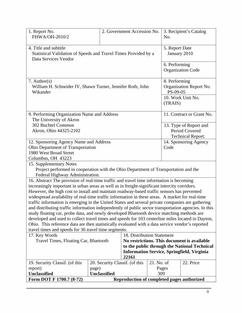
16. Abstract The provision of real-time traffic and travel time information is becoming increasingly important in urban areas as well as in freight-significant intercity corridors. However, the high cost to install and maintain roadway-based traffic sensors has prevented widespread availability of real-time traffic information in these areas. A market for real-time traffic information is emerging in the United States and several private companies are gathering and distributing traffic information independently of public sector transportation agencies. In this study floating car, probe data, and newly developed Bluetooth device matching methods are developed and used to collect travel times and speeds for 103 centerline miles located in Dayton, Ohio. This reference data are then statistically evaluated with a data service vendor’s reported travel times and speeds for 36 travel time segments. 17. Key Words

Travel Times, Floating Car, Bluetooth 18. Distribution Statement No restrictions. This document is available to the public through the National Technical Information Service, Springfield, Virginia 22161

19. Security Classif. (of this report) Unclassified

20. Security Classif. (of this page) Unclassified

21. No. of Pages

309

22. Price

Form DOT F 1700.7 (8-72) Reproduction of completed pages authorized

Final Report iii

STATISTICAL VALIDATION OF SPEEDS AND TRAVEL TIMES PROVIDED

BY A DATA SERVICES VENDOR

By William H. Schneider IV, Ph.D., P.E.,

Jennifer Roth Department of Civil Engineering

The University of Akron

And

Shawn Turner P.E., John Wikander

Texas Transportation Institute

Report Date: January 2010

Prepared in cooperation with the Ohio Department of Transportation

and the U.S. Department of Transportation, Federal Highway Administration

Final Report iv

DISCLAIMER

The contents of this report reflect the views of the authors, who are responsible for the facts and the

accuracy of the data presented herein. The contents do not necessarily reflect the official view of policies

of the Ohio Department of Transportation (ODOT) of the Federal Highway Administration (FHWA).

This report does not constitute a standard, specification or regulation.

Final Report v

ACKNOWLEDGMENTS

This project was conducted in cooperation with ODOT and FHWA.

The authors would like to thank the members of ODOT’s Technical Liaison Committee:

• Mr. George Saylor, ODOT Office of Traffic Engineering,

• Ms. Marian Thompson, ODOT Office of Traffic Engineering, and

• Mr. Bryan Comer, ODOT Office of Traffic Engineering.

Their time and help were greatly appreciated. In addition to our technical liaisons, the authors would like

to thank Ms. Monique Evans, Ms. Vicky Fout and Ms. Jill Martindale from ODOT’s Office of Research

and Development. Their time and help were greatly appreciated. The authors would like to thank Mr.

Kevin Fraleigh, Mr. Darren N. Moore, Mr. John Less, and Mr. James Henry of The University of Akron

for their help on this project. The authors would also like to thank Mr. Darryl Puckett of the Texas

Transportation Institute for his guidance with data collection methodologies.

Final Report vi

TABLE OF CONTENTS

Page

LIST OF APPENDICES ................................................................................................................ ix

LIST OF TABLES .......................................................................................................................... x

LIST OF FIGURES ..................................................................................................................... xiv

LIST OF EQUATIONS ................................................................................................................ xix

LIST OF ACRONYMS ................................................................................................................ xx

CHAPTER

I. INTRODUCTION………………….……………….…………………......……… .................... 1

1.1 Purpose and Research Objectives ……………………………………… ........... …….1

1.2 Benefits from this Research ……………………………………………… ............ ….2

1.3 Organization of this Report ……………………………………………… ............ …..3

II. LITERATURE REVIEW ........................................................................................................... 4

2.1 Introduction .................................................................................................................. 4

2.2 Data Collection Methodology ...................................................................................... 4

2.2.1 Test Vehicle Techniques .................................................................................... 5

2.2.2 License Plate Matching Technique .................................................................... 7

2.2.3 Other Techniques Used ...................................................................................... 7

2.2.4 Probe Vehicle Sample Sizes ............................................................................... 8

2.2.5 Bluetooth Devices ........................................................................................... 10

2.3 Summary of the Data Collection Methodologies ....................................................... 11

III. METHODOLOGY ................................................................................................................. 12

3.1 Introduction ................................................................................................................ 12

3.2 Location of Data Collection ....................................................................................... 12

3.3 Temporal Data Collection .......................................................................................... 13

3.3.1 Trip One ........................................................................................................... 15

3.3.2 Trip Two ........................................................................................................... 15

3.3.3 Trip Three ......................................................................................................... 15

3.3.4 Trip Four .......................................................................................................... 16

Final Report vii

3.3.5 Trip Five ........................................................................................................... 16

3.4 Data Collection Methodology .................................................................................... 16

3.4.1 Spot Speed Method .......................................................................................... 16

3.4.2 Floating Car Method ........................................................................................ 17

3.4.3 Bluetooth Method ............................................................................................. 19

3.5 Roadway Characteristics ............................................................................................ 22

3.5.1 Interstate Highways .......................................................................................... 22

3.5.2 Other Roadways ............................................................................................... 32

3.6 Data Cleaning and Quality Control ............................................................................ 38

3.7 Summary of Data Collection Methods ....................................................................... 41

IV. RESULTS .............................................................................................................................. 43

4.1 Comparison between the Spot Speed Readings and Sensor Speeds .......................... 43

4.1.1 Discussion of Results ....................................................................................... 46

4.2 Comparison of Bluetooth and Floating Car Methods ................................................ 46

4.2.1 High Volume Roads ......................................................................................... 47

4.2.2 Low Volume Roads .......................................................................................... 50

4.2.3 Implementation of Bluetooth based on Time of Day ....................................... 52

4.2.4 Work Zone Related Congestion ....................................................................... 53

4.2.5 Summary of Results ......................................................................................... 54

4.3 ODOT Travel Time Data Compression ..................................................................... 54

4.3.1 Free-flow Conditions ......................................................................................... 55

4.3.2 Periods of Congestion ....................................................................................... 59

4.3.3 Advantages of Bluetooth Method ..................................................................... 61

4.3.4 Underreported Travel Times ............................................................................. 64

4.3.5 Effects of Travel Time Rounding on Short Segments ....................................... 68

4.3.6 Occurrence of Unexplained Differences in Reported Travel Time ................... 70

4.4 Summary of Findings .................................................................................................. 74

V. CONCLUSIONS AND RECOMMENDATIONS ................................................................. 78

5.1 Introduction ................................................................................................................ 78

5.2 Comparison Between Spot Speed Readings and Sensor Speeds ............................... 78

5.3 Evaluation of Bluetooth and Floating Car Methods ................................................... 79

5.3.1 High Volume Access-Controlled Interstate Highways ..................................... 80

Final Report viii

5.3.2 Arterial Highways ............................................................................................. 80

5.4 The Statistical Evaluation of ODOT Travel Times and

Speeds with Field Reference Data .............................................................................. 81

5.4.1 Free-flow Conditions ......................................................................................... 81

5.4.2 Periods of Congestion ....................................................................................... 82

5.4.3 Data Resolution using Bluetooth Method in

Addition to the Floating Car Method................................................................ 82

5.4.4 The Underreporting of Travel Times,

Especially on Arterial Highways ...................................................................... 82

5.4.5 Rounding Travel Times to the Nearest

Minute on Short Segment Lengths ................................................................... 82

5.4.6 Unexplained Differences in Reported Travel Times ......................................... 83

5.5 Conclusion Summary ................................................................................................. 84

VI. RECOMMENDATION FOR IMPLEMENTATION PLAN ................................................. 85

6.1 Recommendations for Implementation ...................................................................... 85

6.2 Steps Needed to Implement Findings ........................................................................ 85

6.3 Suggested Time Frame for Implementation ............................................................... 86

6.4 Expected Benefits from Implementation .................................................................... 86

6.5 Potential Risks and Obstacles to Implementation ....................................................... 86

6.6 Strategies to Overcome Potential Risks and Obstacles ............................................... 87

6.7 Potential Users and Other Organizations that May be Affected ................................. 87

6.8 Estimated Costs of Implementation ............................................................................ 87

VII. REFERENCES ...................................................................................................................... 89

Final Report ix

LIST OF APPENDICES .......................................................................................................... Page

Appendix A: Spot Speeds ........................................................................................................ 93

Appendix B: Histograms ....................................................................................................... 123

Appendix C: Bluetooth Floating Car Comparison ................................................................ 130

Appendix D: Statistical Evaluation of ODOT Travel Times and Reference Data ................ 166

Final Report x

LIST OF TABLES ..................................................................................................................... Page

2.1. Test vehicle data collection techniques used to evaluate travel time accuracy ................... 6

2.2. License plate matching techniques used to evaluate travel time accuracy ........................... 7

2.3. Other techniques used to evaluate travel time accuracy ...................................................... 8

2.4. Research of probe vehicle sample sizes ............................................................................... 9

3.1. Slow speed data .................................................................................................................. 15

3.2. Sample data logger output data set ..................................................................................... 18

3.3. Travel time Segment data collection summary for I-70 ..................................................... 24

3.4. Travel time Segment data collection summary for I-75 ..................................................... 28

3.5. Travel time Segment data collection summary for I-675 ................................................... 32

3.6. Travel time Segment data collection summary for US-35 ................................................. 34

3.7. Travel time Segment data collection summary for SR-49 ................................................. 36

3.8. Travel time Segment data collection summary for SR-4 ................................................... 38

3.9. Example of unreasonable speeds obtained on SR-49 ......................................................... 39

3.10. Summary of travel time Segment coverage ..................................................................... 42

4.1. Summary of results, Segment 3 ......................................................................................... 56

4.2. Summary of results, Segment 21 ....................................................................................... 58


4.4. Summary of results, Segment 9 ......................................................................................... 62






4.10. Summary of results for access-controlled interstate highways (I-70, I-75, I-675) ........... 75

4.11. Summary of results for arterial streets and highways (US 35, SR 4, SR 49) ................... 75

4.12. General summary of results for all travel time Segments included in this study ............. 76

A.1. Raw data ID number 10681 .............................................................................................. 94






A.7. Raw data ID number 10003 ............................................................................................ 100

Final Report xi




A.11. Raw data ID number 11120 .......................................................................................... 104



















D.1. Summary of Segment 1 ................................................................................................... 167









D.10. Summary of Segment 10 ............................................................................................... 176



Final Report xii

























Final Report xiii

LIST OF FIGURES ................................................................................................................... Page

3.1. Study area aerial photograph .............................................................................................. 13

3.2. Peak period traffic flow ...................................................................................................... 14

3.3. Floating car method equipment .......................................................................................... 17

3.4. Depicts the equipment utilized for the Bluetooth method .................................................. 21

3.5. Data location setup for I-70 ................................................................................................ 23

3.6. Data collection location north of Dayton, July 2009 ......................................................... 25

3.7. Data collection location north of Dayton ........................................................................... 26

3.8. Data collection location south of Dayton ........................................................................... 27

3.9. I-675 data collection north of US-35 ................................................................................. 29

3.10. I-675 data collection south of US-35 ............................................................................... 31

3.11. US-35 data collection ....................................................................................................... 33

3.12. Data collection located on SR-49 ..................................................................................... 35

3.13. SR-4 data collection ......................................................................................................... 37

3.14. Example of outliers within Bluetooth method data .......................................................... 40

3.15. Example of widely varying floating car speeds and Bluetooth speeds ............................ 41

4.1. Device number 10681, I-70, 7/27/2009, morning rush hour .............................................. 44

4.2. Device number 10691, I-70, 7/27/2009, morning rush hour .............................................. 45

4.3. Device number 10777, I-76, 8/17/2009, afternoon rush hour ............................................ 45

4.4. Summary of speed differential across all radar sensor locations ....................................... 46

4.5. Travel time Segment ID 1, 7/27/2009, afternoon rush hour .............................................. 48

4.6. Travel time Segment ID 10, 7/29/2009, afternoon rush hour ............................................ 49




4.10. Travel time Segment ID 28, 8/19/2009, PM .................................................................... 53


4.12. Travel time according to time of day, Segment 3 ............................................................ 57

4.13. Speed according to time of day, Segment 3 ..................................................................... 57

4.14. Travel time according to time of day, Segment 21 .......................................................... 58

4.15. Speed according to time of day, Segment 21 ................................................................... 59



4.18. Travel time according to time of day, Segment 9 ............................................................ 63

Final Report xiv

4.19. Speed according to time of day, Segment 9 ..................................................................... 64











B.1. Histogram for ID number 10681. .................................................................................... 124

B.2. Histogram for ID number 10691 ..................................................................................... 124








B.10. Histogram for ID number 10870 ................................................................................... 128





C.1. Travel time Segment ID 1, 7/27/2009, PM ..................................................................... 131






C.7. Travel time Segment ID 9, 7/29/2009, AM ..................................................................... 134


C.9. Travel time Segment ID 10, 7/29/2009, AM. .................................................................. 135

Final Report xv

C.10. Travel time Segment ID 10, 7/29/2009, PM ................................................................. 135

C.11. Travel time Segment ID 11, 7/29/2009, AM. ................................................................ 136








C.19. Travel time Segment ID 13, 9/3/2009, AM ................................................................... 140

























Final Report xvi



























D.1. Individual comparison Segment 1 ................................................................................... 167








Final Report xvii


D.10. Individual comparison Segment 10 ............................................................................... 176



























Final Report xviii

LIST OF EQUATIONS ............................................................................................................ Page

3.1 .............................................................................................................................................. 19

3.2 .............................................................................................................................................. 19

3.3 .............................................................................................................................................. 19

3.4 .............................................................................................................................................. 20

Final Report xix

LIST OF ACRONYMS

AADT Annual Average Daily Traffic

AASHTO American Association of State Highway and Transportation

Officials

AATT Applications of Advanced Technology in Transportation

ABJ20 TRB Statewide Transportation Data and Information Systems Committee

ADA70 TRB Access Management Committee

ADT Average Daily Traffic

ANN Artificial Neural Network

APBP Association of Pedestrian and Bicycle Professionals

ASTM American Society for Testing Materials

ATIS Advanced Traveler Information System

ATR Automatic Traffic Recorder

AVL Automatic Vehicle Location

CCIT California Center for Innovative Transportation

Co-PI Co-Principal Investigator

COV Coefficient of Variation

CPI Council of Principal Investigators

DMI Distance Measuring Instrument

DOT Department of Transportation

DPS Department of Public Safety

FHWA Federal Highway Administration

GIS Geographic Information Systems

GPS Global Positioning System

Final Report xx

LIST OF ACRONYMS (continued)

HOV High Occupancy Vehicles

HSM Highway Safety Manual

ITE Institute of Transportation Engineers

ITS Intelligent Transportation Systems

MPO Metropolitan Planning Organization

NATMEC North American Traffic Monitoring Exhibition and Conference

NCHRP National Cooperative Highway Research Program

ODOT Ohio Department of Transportation or Oregon Department of

Transportation

PE Professional Engineer

PI Principal Investigator

R&D Research and Development

RFID Radio Frequency Identifier

SAF Seasonal Adjustment Factor

SD Standard Deviation

SMSC Small to Medium-Sized Communities

SWUTC Southwestern Region University Transportation Center

TAMUS Texas A&M University System

TexITE Institute of Transportation Engineers, National and Texas Section

TRB Transportation Research Board

TTECP Travel Time Estimation Using Cell Phones

TTI Texas Transportation Institute

TxDOT Texas Department of Transportation

UC-Berkeley University of California Berkeley

VISSIM Visual Solutions Transportation Simulation Software

Final Report xxi

LIST OF ACRONYMS (continued)

VTRC Virginia Transportation Research Council

Final Report xxii

Customary Unit SI Unit Factor SI Unit Customary

Unit Factor

Length Length

inches millimeters 25.4 millimeters inches 0.039 inches centimeters 2.54 centimeters inches 0.394

feet meters 0.305 meters feet 3.281 yards meters 0.914 meters yards 1.094 miles kilometers 1.61 kilometers miles 0.621

Area Area square inches

square millimeters 645.1 square

millimeters square inches 0.00155

square feet square meters 0.093 square

meters square feet 10.764

square yards square meters 0.836 square

meters square yards 1.196

acres hectares 0.405 hectares acres 2.471

square miles square kilometers 2.59 square

kilometers square miles 0.386

Volume Volume gallons liters 3.785 liters gallons 0.264

cubic feet cubic meters 0.028 cubic meters cubic feet 35.314 cubic yards cubic meters 0.765 cubic meters cubic yards 1.308

Mass Mass ounces grams 28.35 grams ounces 0.035 pounds kilograms 0.454 kilograms pounds 2.205

short tons megagrams 0.907 megagrams short tons 1.102

Final Report 1

CHAPTER I

INTRODUCTION

The provision of real-time traffic and travel time information is becoming increasingly

important in urban areas as well as in freight-significant intercity corridors. However, the high

cost to install and maintain roadway-based traffic sensors has prevented widespread availability

of real-time traffic information in these areas. A market for real-time traffic information is

emerging in the United States and several private companies are gathering and distributing traffic

information independently of public sector transportation agencies. In fact, several of these

private companies have begun marketing their traffic information to public sector agencies like

state departments of transportation (DOTs).

The problem is that some private companies are still developing and/or refining their

traffic monitoring technology, whether it is Global Positioning Systems (GPS), probe vehicles or

cell phones methods, while at the same time trying to sell the technology as a mature product. For

example, several evaluations of cell phone-based traffic monitoring in the past five years have

provided poor results. Based on these findings, it is critical that the quality of private sector travel

time data be adequately evaluated in fee-for-service contracts with state DOTs.

1.1 Purpose and Objectives

There are four research objectives, which must be met in order to insure that project PS-09-05

“Statistical Validation of Speeds and Travel Times Provided by a Data Services Vendor” will be

considered a success as described in the request for proposal. These four objectives include:

• Objective One - Conduct a data collection GPS floating car methodology along

103 centerline miles (165.8 km) in Dayton, Ohio,

• Objective Two - Evaluate the accuracy of travel time data from a service provider,

• Objective Three - Provide recommendations for travel time data service evaluation

procedures to be used in contract provisions and/or future

evaluations, and

• Objective Four - Summarize the final results.

1.2 Benefits from this Research

Final Report 2

The research described within this report will have both immediate as well as long-term

benefits. The immediate benefit of this research project is an assurance that the travel time data

service does, or does not, meet contract requirements. If the travel time data service does not meet

contract requirements, then Ohio Department of Transportation (ODOT) may not be legally

obligated to pay the data service provider. If the travel time data service does meet contract

requirements, then ODOT will be assured that state funds have been well spent in acquiring this

data service. An additional short-term benefit for ODOT will be the external review of the data.

This external review ensures the accuracy of the data, strengthening the initiative’s credibility

with the public as well as the media. This research will allow ODOT the capability to say an

external agency has reviewed and implemented quality control/quality assurance procedures on

all data provided from the external vendor.

The main long-term benefit is that ODOT may save money and provide this service much

sooner than otherwise possible by purchasing this real-time traffic information service from a

private company instead of installing and maintaining a state-owned traffic sensor network.

The overall findings from this research will provide a long-term cost savings for ODOT

whether the vendor’s travel time data are accurate or inaccurate. If the data are proven accurate,

ODOT will be able to use this information to provide reliable travel time information both

internally and externally and will lead to a cost savings. If the research proves the data provided

by the vendor are inaccurate, ODOT will no longer use this vendor or pay for services that are

invalid. The potential benefit to cost ratio of this project is based predominately on three cost

saving objectives:

• Cost Savings Number One – the potential agency cost savings through private

company installation of the network over state-owned

traffic sensors,

• Cost Savings Number Two – the potential travel time savings for the individual user,

and

• Cost Savings Number Three – efficiently evaluate vendor’s data service.

The actual benefit to cost ratio may be hard to define without the contractual numbers

provided by the data vendor, but based on the three described cost savings there is potential for a

higher benefit to cost ratio from this research.

1.3 Organization of this Report

Final Report 3

This report is divided into six chapters. The first chapter is the introduction of the topic

and the statement of the research objectives. The second chapter is the literature review. The

literature review will provide the state-of-the-practice for the collection and analysis of speed and

travel time data. The third chapter is the research methodology used with collecting the

appropriate data for use in the analysis. The fourth chapter is the summary of the results from the

data collection. These results will include the average speeds and travel times for the segments of

the highway. Additional results include the comparison between the travel times provided by a

data service provider and the ground truth results developed from the data collection. The fifth

chapter of this report will provide conclusions and recommendations, which are based on the final

results. The last chapter will provide suggestions on the best approach to implement the findings

from this research.

Final Report 4

CHAPTER II

LITERATURE REVIEW

2.1 Introduction

Numerous evaluations of travel time accuracy have been performed in recent years.

These evaluations include a wide variety of approaches and data collection parameters to

establish travel time accuracy. The most common approach, however, has been to drive one or

more GPS-instrumented test vehicles along the roadway or street to be evaluated. Beyond that,

many of the details vary considerably, including the headway or spacing if more than one vehicle

is used, the number of road segments that should be sampled and the number of days and time

periods that should be sampled.

In many evaluations, it appears that sampling parameters are based on the available

evaluation budget and not necessarily statistical significance. Often, the evaluation team provides

no confidence interval to reinforce the accuracy of their “ground truth” travel time. In some

evaluations, the evaluators are not truly independent because they are paid by the private

company providing the travel time service. A recent report from National Cooperative Highway

Research Program (NCHRP) Project 70-01 provides some insight about the data quality

requirements that should be included in a fee-for-service contract with the private sector, but

ultimately this report does not provide many data collection and analysis details regarding how to

determine whether the private contractor has met these requirements.

With the growth of the real-time traffic information market in the United States, several

private companies are aggressively developing traveler information products. Several of these

private companies are concerned about the consistency of evaluations and are discussing the

possibility of a national or international standard protocol for travel time evaluation. Such a

standard would include detailed procedures for evaluating the accuracy of travel time data

services. This evaluation protocol standard could then be specified when state DOTs issue a

request for proposals or when they sign fee-for-service contracts. If developed, this standard

could provide a “level playing field” by which all travel time data service providers could be

evaluated and compared.

2.2 Data Collection Methodology

There are two solution types to determine the true average travel time for all vehicles

traversing a designated length of roadway for a fixed time period:

Final Report 5

• Cost-Not-An-Issue Solution - Identify and re-identify (using license plate matching,

radio frequency identifier (RFID) tags, GPS receivers, etc.) each vehicle that traverses

the designated length of roadway during the fixed time period. This is commonly

referred to as the “platinum standard” for ground truth travel time measurement, and

• Feasible Near-Term Solutions - Identify and re-identify a statistically valid sample of

vehicles. This is referred to as a “gold standard” for ground truth travel time

measurement. Alternatively, to use a test vehicle at frequent headways to obtain a

statistically valid sample to simplify the identification and re-identification of vehicles

in the traffic stream is referred to as the “silver standard” for ground truth travel time

measurement.

Various approaches are used to evaluate the accuracy of estimated or predicted travel times.

Tables 2.1 through 2.4 summarize these test methods for travel time accuracy evaluation.

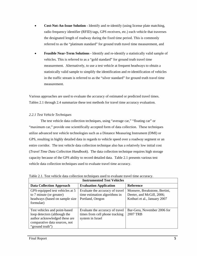
2.2.1 Test Vehicle Techniques

The test vehicle data collection techniques, using “average car,” “floating car” or

“maximum car,” provide one scientifically accepted form of data collection. These techniques

utilize advanced test vehicle technologies such as a Distance Measuring Instrument (DMI) or

GPS, resulting in highly detailed data in regards to vehicle speed over a roadway segment or an

entire corridor. The test vehicle data collection technique also has a relatively low initial cost

(Travel Time Data Collection Handbook). The data collection technique requires high storage

capacity because of the GPS ability to record detailed data. Table 2.1 presents various test

vehicle data collection techniques used to evaluate travel time accuracy.

Table 2.1. Test vehicle data collection techniques used to evaluate travel time accuracy. Instrumented Test Vehicles

Data Collection Approach Evaluation Application Reference GPS-equipped test vehicles at 5 to 7 minute (or greater) headways (based on sample size formulae)

Evaluate the accuracy of travel time estimation algorithms in Portland, Oregon

Monsere, Breakstone, Bertini, Deeter, and McGill, 2006; Kothuri et al., January 2007

Test vehicles and point-based loop detectors (although the author acknowledged these are comparative data sources, not “ground truth”)

Evaluate the accuracy of travel times from cell phone tracking system in Israel

Bar-Gera, November 2006 for 2007 TRB

Final Report 6

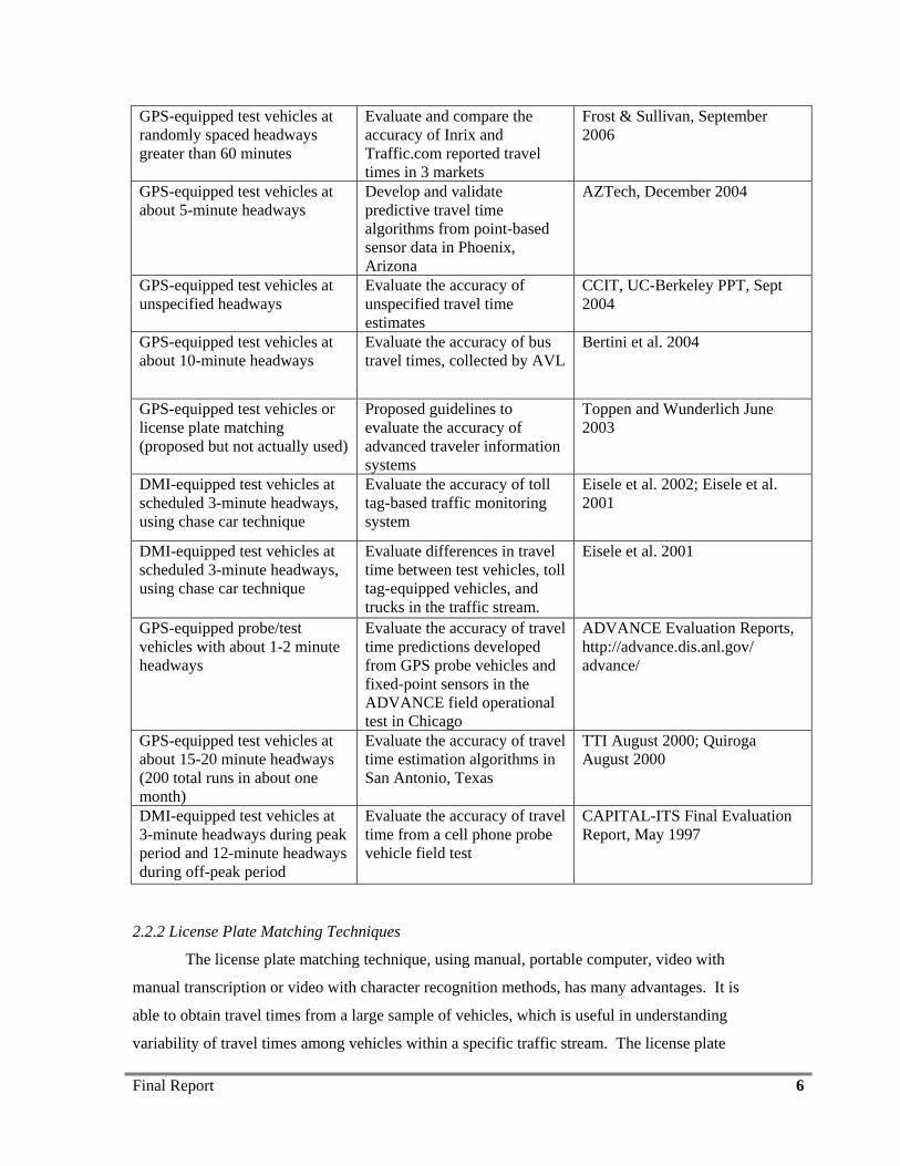
GPS-equipped test vehicles at randomly spaced headways greater than 60 minutes

Evaluate and compare the accuracy of Inrix and Traffic.com reported travel times in 3 markets

Frost & Sullivan, September 2006

GPS-equipped test vehicles at about 5-minute headways

Develop and validate predictive travel time algorithms from point-based sensor data in Phoenix, Arizona

AZTech, December 2004

GPS-equipped test vehicles at unspecified headways

Evaluate the accuracy of unspecified travel time estimates

CCIT, UC-Berkeley PPT, Sept 2004

GPS-equipped test vehicles at about 10-minute headways

Evaluate the accuracy of bus travel times, collected by AVL

Bertini et al. 2004

GPS-equipped test vehicles or license plate matching (proposed but not actually used)

Proposed guidelines to evaluate the accuracy of advanced traveler information systems

Toppen and Wunderlich June 2003

DMI-equipped test vehicles at scheduled 3-minute headways, using chase car technique

Evaluate the accuracy of toll tag-based traffic monitoring system

Eisele et al. 2002; Eisele et al. 2001

DMI-equipped test vehicles at scheduled 3-minute headways, using chase car technique

Evaluate differences in travel time between test vehicles, toll tag-equipped vehicles, and trucks in the traffic stream.

Eisele et al. 2001

GPS-equipped probe/test vehicles with about 1-2 minute headways

Evaluate the accuracy of travel time predictions developed from GPS probe vehicles and fixed-point sensors in the ADVANCE field operational test in Chicago

ADVANCE Evaluation Reports, http://advance.dis.anl.gov/ advance/

GPS-equipped test vehicles at about 15-20 minute headways (200 total runs in about one month)

Evaluate the accuracy of travel time estimation algorithms in San Antonio, Texas

TTI August 2000; Quiroga August 2000

DMI-equipped test vehicles at 3-minute headways during peak period and 12-minute headways during off-peak period

Evaluate the accuracy of travel time from a cell phone probe vehicle field test

CAPITAL-ITS Final Evaluation Report, May 1997

2.2.2 License Plate Matching Techniques

The license plate matching technique, using manual, portable computer, video with

manual transcription or video with character recognition methods, has many advantages. It is

able to obtain travel times from a large sample of vehicles, which is useful in understanding

variability of travel times among vehicles within a specific traffic stream. The license plate

Final Report 7

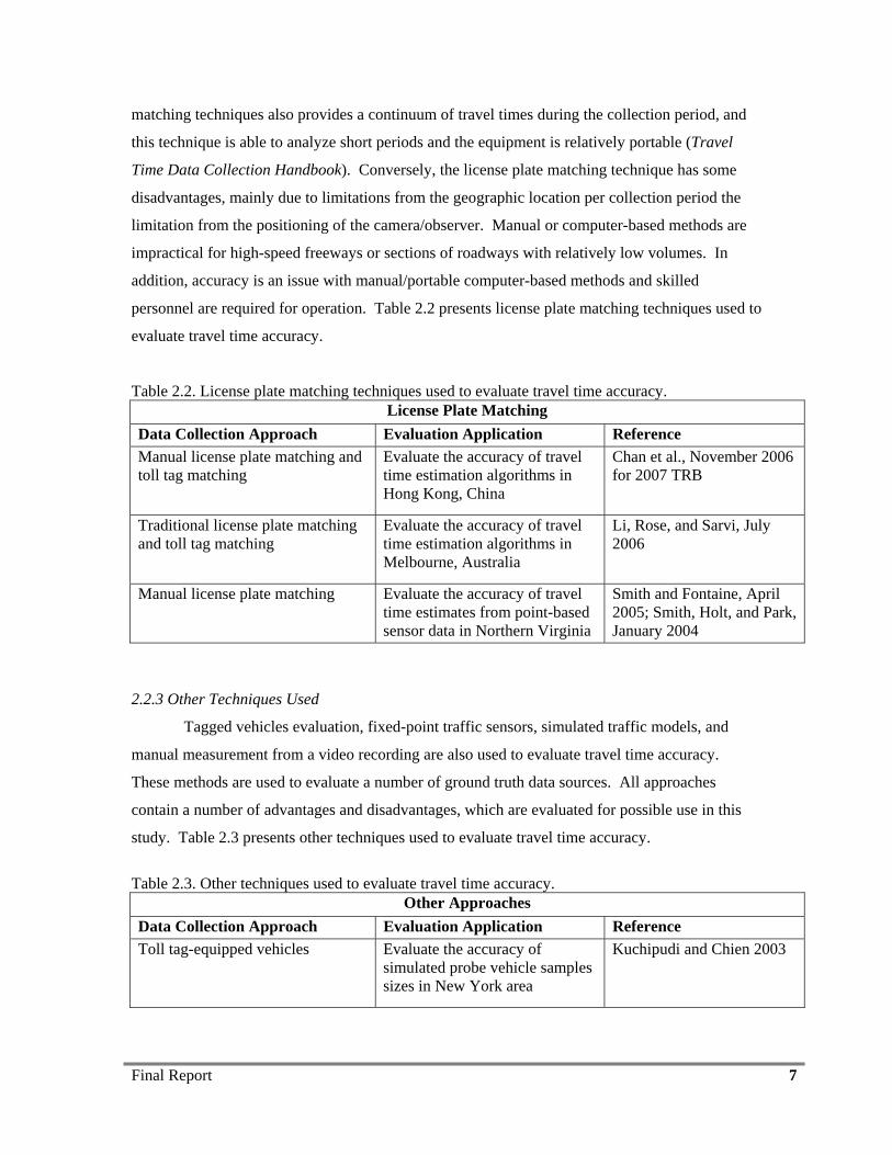
matching techniques also provides a continuum of travel times during the collection period, and

this technique is able to analyze short periods and the equipment is relatively portable (Travel

Time Data Collection Handbook). Conversely, the license plate matching technique has some

disadvantages, mainly due to limitations from the geographic location per collection period the

limitation from the positioning of the camera/observer. Manual or computer-based methods are

impractical for high-speed freeways or sections of roadways with relatively low volumes. In

addition, accuracy is an issue with manual/portable computer-based methods and skilled

personnel are required for operation. Table 2.2 presents license plate matching techniques used to

evaluate travel time accuracy.

Table 2.2. License plate matching techniques used to evaluate travel time accuracy. License Plate Matching

Data Collection Approach Evaluation Application Reference Manual license plate matching and toll tag matching

Evaluate the accuracy of travel time estimation algorithms in Hong Kong, China

Chan et al., November 2006 for 2007 TRB

Traditional license plate matching and toll tag matching

Evaluate the accuracy of travel time estimation algorithms in Melbourne, Australia

Li, Rose, and Sarvi, July 2006

Manual license plate matching Evaluate the accuracy of travel time estimates from point-based sensor data in Northern Virginia

Smith and Fontaine, April 2005; Smith, Holt, and Park, January 2004

2.2.3 Other Techniques Used

Tagged vehicles evaluation, fixed-point traffic sensors, simulated traffic models, and

manual measurement from a video recording are also used to evaluate travel time accuracy.

These methods are used to evaluate a number of ground truth data sources. All approaches

contain a number of advantages and disadvantages, which are evaluated for possible use in this

study. Table 2.3 presents other techniques used to evaluate travel time accuracy.

Table 2.3. Other techniques used to evaluate travel time accuracy.

Other Approaches Data Collection Approach Evaluation Application Reference Toll tag-equipped vehicles Evaluate the accuracy of

simulated probe vehicle samples sizes in New York area

Kuchipudi and Chien 2003

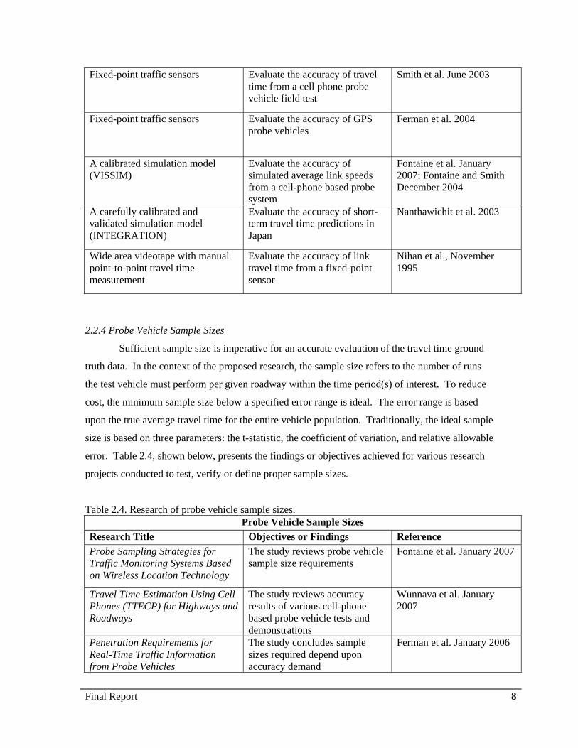
Final Report 8

Fixed-point traffic sensors Evaluate the accuracy of travel time from a cell phone probe vehicle field test

Smith et al. June 2003

Fixed-point traffic sensors Evaluate the accuracy of GPS probe vehicles

Ferman et al. 2004

A calibrated simulation model (VISSIM)

Evaluate the accuracy of simulated average link speeds from a cell-phone based probe system

Fontaine et al. January 2007; Fontaine and Smith December 2004

A carefully calibrated and validated simulation model (INTEGRATION)

Evaluate the accuracy of short-term travel time predictions in Japan

Nanthawichit et al. 2003

Wide area videotape with manual point-to-point travel time measurement

Evaluate the accuracy of link travel time from a fixed-point sensor

Nihan et al., November 1995

2.2.4 Probe Vehicle Sample Sizes

Sufficient sample size is imperative for an accurate evaluation of the travel time ground

truth data. In the context of the proposed research, the sample size refers to the number of runs

the test vehicle must perform per given roadway within the time period(s) of interest. To reduce

cost, the minimum sample size below a specified error range is ideal. The error range is based

upon the true average travel time for the entire vehicle population. Traditionally, the ideal sample

size is based on three parameters: the t-statistic, the coefficient of variation, and relative allowable

error. Table 2.4, shown below, presents the findings or objectives achieved for various research

projects conducted to test, verify or define proper sample sizes.

Table 2.4. Research of probe vehicle sample sizes. Probe Vehicle Sample Sizes

Research Title Objectives or Findings Reference Probe Sampling Strategies for Traffic Monitoring Systems Based on Wireless Location Technology

The study reviews probe vehicle sample size requirements

Fontaine et al. January 2007

Travel Time Estimation Using Cell Phones (TTECP) for Highways and Roadways

The study reviews accuracy results of various cell-phone based probe vehicle tests and demonstrations

Wunnava et al. January 2007

Penetration Requirements for Real-Time Traffic Information from Probe Vehicles

The study concludes sample sizes required depend upon accuracy demand

Ferman et al. January 2006

Final Report 9

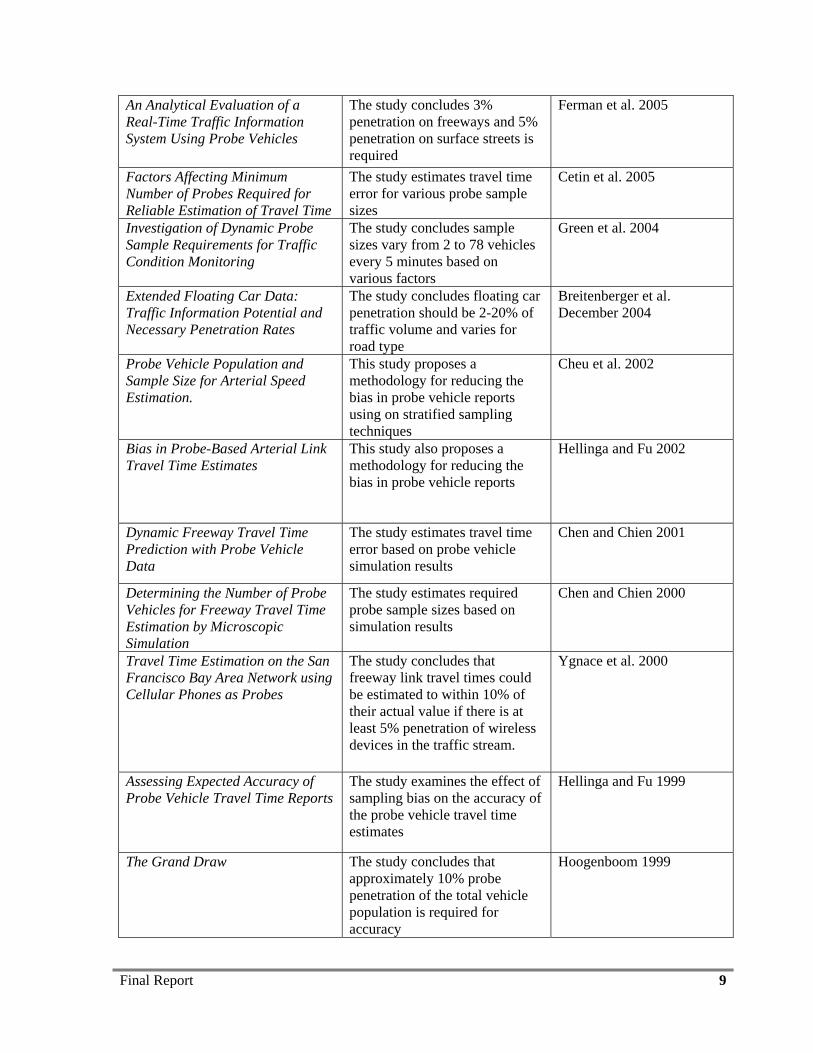
An Analytical Evaluation of a Real-Time Traffic Information System Using Probe Vehicles

The study concludes 3% penetration on freeways and 5% penetration on surface streets is required

Ferman et al. 2005

Factors Affecting Minimum Number of Probes Required for Reliable Estimation of Travel Time

The study estimates travel time error for various probe sample sizes

Cetin et al. 2005

Investigation of Dynamic Probe Sample Requirements for Traffic Condition Monitoring

The study concludes sample sizes vary from 2 to 78 vehicles every 5 minutes based on various factors

Green et al. 2004

Extended Floating Car Data: Traffic Information Potential and Necessary Penetration Rates

The study concludes floating car penetration should be 2-20% of traffic volume and varies for road type

Breitenberger et al. December 2004

Probe Vehicle Population and Sample Size for Arterial Speed Estimation.

This study proposes a methodology for reducing the bias in probe vehicle reports using on stratified sampling techniques

Cheu et al. 2002

Bias in Probe-Based Arterial Link Travel Time Estimates

This study also proposes a methodology for reducing the bias in probe vehicle reports

Hellinga and Fu 2002

Dynamic Freeway Travel Time Prediction with Probe Vehicle Data

The study estimates travel time error based on probe vehicle simulation results

Chen and Chien 2001

Determining the Number of Probe Vehicles for Freeway Travel Time Estimation by Microscopic Simulation

The study estimates required probe sample sizes based on simulation results

Chen and Chien 2000

Travel Time Estimation on the San Francisco Bay Area Network using Cellular Phones as Probes

The study concludes that freeway link travel times could be estimated to within 10% of their actual value if there is at least 5% penetration of wireless devices in the traffic stream.

Ygnace et al. 2000

Assessing Expected Accuracy of Probe Vehicle Travel Time Reports

The study examines the effect of sampling bias on the accuracy of the probe vehicle travel time estimates

Hellinga and Fu 1999

The Grand Draw The study concludes that approximately 10% probe penetration of the total vehicle population is required for accuracy

Hoogenboom 1999

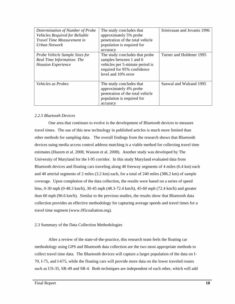
Final Report 10

Determination of Number of Probe Vehicles Required for Reliable Travel Time Measurement in Urban Network

The study concludes that approximately 5% probe penetration of the total vehicle population is required for accuracy

Srinivasan and Jovanis 1996

Probe Vehicle Sample Sizes for Real Time Information: The Houston Experience

The study concludes that probe samples between 1 and 6 vehicles per 5-minute period is required for 95% confidence level and 10% error

Turner and Holdener 1995

Vehicles as Probes The study concludes that approximately 4% probe penetration of the total vehicle population is required for accuracy

Sanwal and Walrand 1995

2.2.5 Bluetooth Devices

One area that continues to evolve is the development of Bluetooth devices to measure

travel times. The use of this new technology in published articles is much more limited than

other methods for sampling data. The overall findings from the research shows that Bluetooth

devices using media access control address matching is a viable method for collecting travel time

estimates (Hazem et al. 2008, Wasson et al. 2008). Another study was developed by The

University of Maryland for the I-95 corridor. In this study Maryland evaluated data from

Bluetooth devices and floating cars traveling along 40 freeway segments of 4 miles (6.4 km) each

and 40 arterial segments of 2 miles (3.2 km) each, for a total of 240 miles (386.2 km) of sample

coverage. Upon completion of the data collection, the results were based on a series of speed

bins, 0-30 mph (0-48.3 km/h), 30-45 mph (48.3-72.4 km/h), 45-60 mph (72.4 km/h) and greater

than 60 mph (96.6 km/h). Similar to the previous studies, the results show that Bluetooth data

collection provides an effective methodology for capturing average speeds and travel times for a

travel time segment (www.i95coaliation.org).

2.3 Summary of the Data Collection Methodologies

After a review of the state-of-the-practice, this research team feels the floating car

methodology using GPS and Bluetooth data collection are the two most appropriate methods to

collect travel time data. The Bluetooth devices will capture a larger population of the data on I-

70, I-75, and I-675, while the floating cars will provide more data on the lower traveled routes

such as US-35, SR-49 and SR-4. Both techniques are independent of each other, which will add

Final Report 11

to better evaluation of ground truth data. These techniques for collecting data will then be

evaluated against travel time data from the data service provider.

Final Report 12

CHAPTER III

METHODOLOGY

3.1 Introduction

The objective of this study is to verify the travel times provided by a data service vendor

located in Dayton, Ohio are accurate. The current system gathers vehicle speed data from radar

sensors located along the highway and uses a variety of algorithms to calculate travel times

between points of interest, based on time-of-day, weather event or other roadway conditions.

When abnormal travel times are reported, common during rain events and congestion, ODOT has

the ability to review real-time video of the corridor in question through Buckeye Travel. The

methodology section is comprised of three data collection components. The first component is

the location of the data collection. The second component is the time-of-day for the data

collection and the third and final component is the method for collecting speed data. Sections 3.2

through 3.4 provide additional information on these components.

3.2 Location of Data Collection

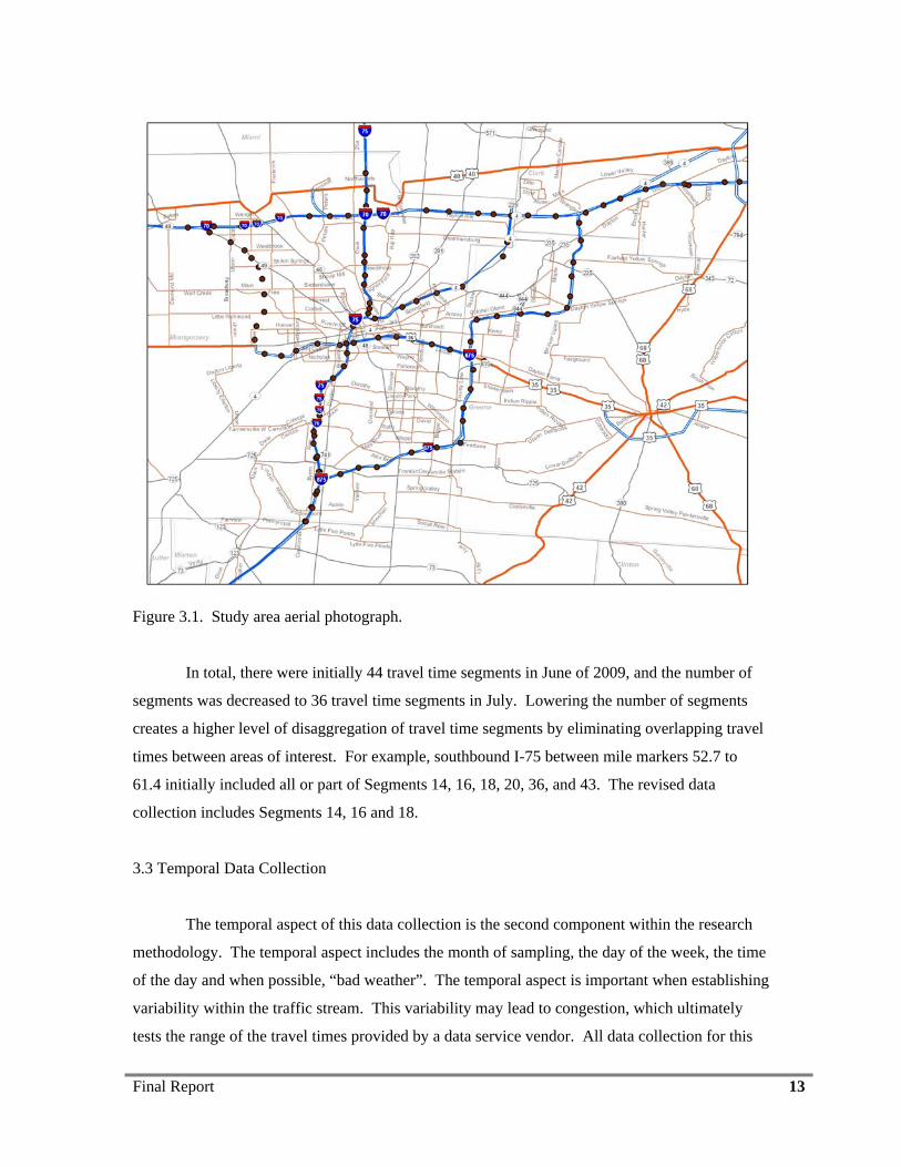
Dayton, Ohio is the location identified by ODOT to study the statistical validation of

travel times provided by a data service vendor. Currently, there are 103 centerline miles (165.8

km) within the Dayton area where travel times are provided. These roadways include:

• I-70 – east westbound between mile markers 25.9 and 47.2,

• I-75 – north and southbound between mile markers 40.9 and 65.3,

• I-675 – north and southbound between mile markers 0.6 and 26.5,

• US-35 – north and southbound between mile markers 30.2 and 41.7,

• SR 49 – north and southbound between mile markers 0.0 and 9, and

• SR 4 – north and southbound between mile markers 16.7 and 27.3.

Final Report 13

Figure 3.1. Study area aerial photograph.

In total, there were initially 44 travel time segments in June of 2009, and the number of

segments was decreased to 36 travel time segments in July. Lowering the number of segments

creates a higher level of disaggregation of travel time segments by eliminating overlapping travel

times between areas of interest. For example, southbound I-75 between mile markers 52.7 to

61.4 initially included all or part of Segments 14, 16, 18, 20, 36, and 43. The revised data

collection includes Segments 14, 16 and 18.

3.3 Temporal Data Collection

The temporal aspect of this data collection is the second component within the research

methodology. The temporal aspect includes the month of sampling, the day of the week, the time

of the day and when possible, “bad weather”. The temporal aspect is important when establishing

variability within the traffic stream. This variability may lead to congestion, which ultimately

tests the range of the travel times provided by a data service vendor. All data collection for this

Final Report 14

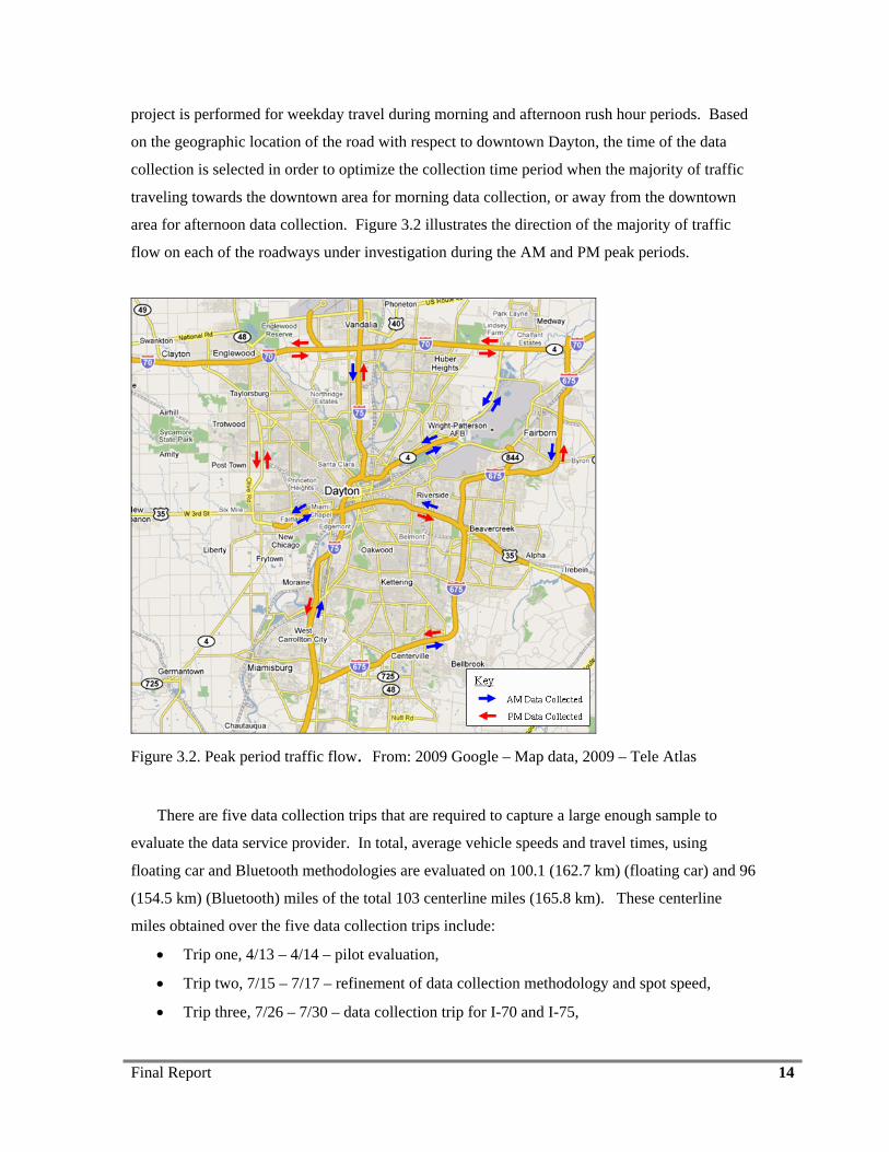
project is performed for weekday travel during morning and afternoon rush hour periods. Based

on the geographic location of the road with respect to downtown Dayton, the time of the data

collection is selected in order to optimize the collection time period when the majority of traffic

traveling towards the downtown area for morning data collection, or away from the downtown

area for afternoon data collection. Figure 3.2 illustrates the direction of the majority of traffic

flow on each of the roadways under investigation during the AM and PM peak periods.

Figure 3.2. Peak period traffic flow. From: 2009 Google – Map data, 2009 – Tele Atlas

There are five data collection trips that are required to capture a large enough sample to

evaluate the data service provider. In total, average vehicle speeds and travel times, using

floating car and Bluetooth methodologies are evaluated on 100.1 (162.7 km) (floating car) and 96

(154.5 km) (Bluetooth) miles of the total 103 centerline miles (165.8 km). These centerline

miles obtained over the five data collection trips include:

• Trip one, 4/13 – 4/14 – pilot evaluation,

• Trip two, 7/15 – 7/17 – refinement of data collection methodology and spot speed,

• Trip three, 7/26 – 7/30 – data collection trip for I-70 and I-75,

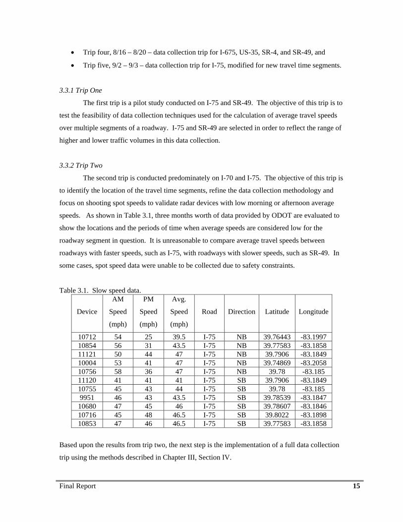
Final Report 15

• Trip four, 8/16 – 8/20 – data collection trip for I-675, US-35, SR-4, and SR-49, and

• Trip five, 9/2 – 9/3 – data collection trip for I-75, modified for new travel time segments.

3.3.1 Trip One

The first trip is a pilot study conducted on I-75 and SR-49. The objective of this trip is to

test the feasibility of data collection techniques used for the calculation of average travel speeds

over multiple segments of a roadway. I-75 and SR-49 are selected in order to reflect the range of

higher and lower traffic volumes in this data collection.

3.3.2 Trip Two

The second trip is conducted predominately on I-70 and I-75. The objective of this trip is

to identify the location of the travel time segments, refine the data collection methodology and

focus on shooting spot speeds to validate radar devices with low morning or afternoon average

speeds. As shown in Table 3.1, three months worth of data provided by ODOT are evaluated to

show the locations and the periods of time when average speeds are considered low for the

roadway segment in question. It is unreasonable to compare average travel speeds between

roadways with faster speeds, such as I-75, with roadways with slower speeds, such as SR-49. In

some cases, spot speed data were unable to be collected due to safety constraints.

Table 3.1. Slow speed data.

Device

AM

Speed

(mph)

PM

Speed

(mph)

Avg.

Speed

(mph)

Road Direction Latitude Longitude

10712 54 25 39.5 I-75 NB 39.76443 -83.1997 10854 56 31 43.5 I-75 NB 39.77583 -83.1858 11121 50 44 47 I-75 NB 39.7906 -83.1849 10004 53 41 47 I-75 NB 39.74869 -83.2058 10756 58 36 47 I-75 NB 39.78 -83.185 11120 41 41 41 I-75 SB 39.7906 -83.1849 10755 45 43 44 I-75 SB 39.78 -83.185 9951 46 43 43.5 I-75 SB 39.78539 -83.1847 10680 47 45 46 I-75 SB 39.78607 -83.1846 10716 45 48 46.5 I-75 SB 39.8022 -83.1898 10853 47 46 46.5 I-75 SB 39.77583 -83.1858

Based upon the results from trip two, the next step is the implementation of a full data collection

trip using the methods described in Chapter III, Section IV.

Final Report 16

3.3.3 Trip Three

The third trip is located exclusively on I-70 and I-75. The objective of this trip is to

collect speed data for both interstate highways based on the June 2009 travel time segments. Trip

three consisted of two data collection periods, morning and afternoon, during the weekday.

3.3.4 Trip Four

The fourth trip is located exclusively on I-675, US-35, SR-4, and SR-49. The objective

of this trip is to collect speed data for the remaining roadways where travel times are reported.

These locations are based on the July 2009 travel time segments. Trip four consists of two

sample periods, morning and afternoon, during the weekday. On one day, data are collected

throughout the evening hours of 8:00 PM until 2:00 AM the following morning. The objective of

this nighttime data collection run is to evaluate the potential effectiveness of Bluetooth data

collection, described in more detail in section 4.2.3, during periods of low volume.

3.3.5 Trip Five

Trip five is the last data collection trip. The objective of trip five is to collect data on I-75

based on the July 2009 travel time segment update. As a result of this trip, additional speed data

are provided for travel time Segments 13 through 20, located on I-75.

3.4 Data Collection Methodology

Three unique and independent data collection methods are used for evaluation purposes

within this study. These data collection methods include spot speed, floating car, and Bluetooth

device identification. While the floating car method is the primary interest, as defined in the

request for proposal, the other two methods are performed in an effort to validate data obtained

from the floating car as well as the data service provider.

3.4.1 Spot Speed Method

The first data collection technique is shooting individual vehicle speeds at fixed locations,

commonly referred to as spot speeds. Spot speed data are an effective method for comparing the

accuracy of individual radar devices. These devices collect the initial data used in the

development of estimated travel times. If these devices are inaccurate, the final travel time will

also be inaccurate. The data collection procedure developed for this project includes shooting

speeds for 25 minutes per direction of travel. This time interval provides a large enough sample

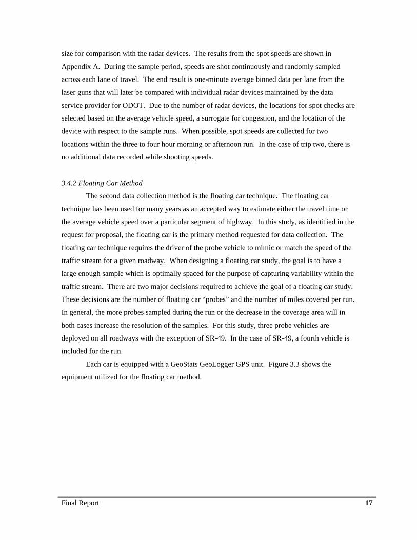
Final Report 17

size for comparison with the radar devices. The results from the spot speeds are shown in

Appendix A. During the sample period, speeds are shot continuously and randomly sampled

across each lane of travel. The end result is one-minute average binned data per lane from the

laser guns that will later be compared with individual radar devices maintained by the data

service provider for ODOT. Due to the number of radar devices, the locations for spot checks are

selected based on the average vehicle speed, a surrogate for congestion, and the location of the

device with respect to the sample runs. When possible, spot speeds are collected for two

locations within the three to four hour morning or afternoon run. In the case of trip two, there is

no additional data recorded while shooting speeds.

3.4.2 Floating Car Method

The second data collection method is the floating car technique. The floating car

technique has been used for many years as an accepted way to estimate either the travel time or

the average vehicle speed over a particular segment of highway. In this study, as identified in the

request for proposal, the floating car is the primary method requested for data collection. The

floating car technique requires the driver of the probe vehicle to mimic or match the speed of the

traffic stream for a given roadway. When designing a floating car study, the goal is to have a

large enough sample which is optimally spaced for the purpose of capturing variability within the

traffic stream. There are two major decisions required to achieve the goal of a floating car study.

These decisions are the number of floating car “probes” and the number of miles covered per run.

In general, the more probes sampled during the run or the decrease in the coverage area will in

both cases increase the resolution of the samples. For this study, three probe vehicles are

deployed on all roadways with the exception of SR-49. In the case of SR-49, a fourth vehicle is

included for the run.

Each car is equipped with a GeoStats GeoLogger GPS unit. Figure 3.3 shows the

equipment utilized for the floating car method.

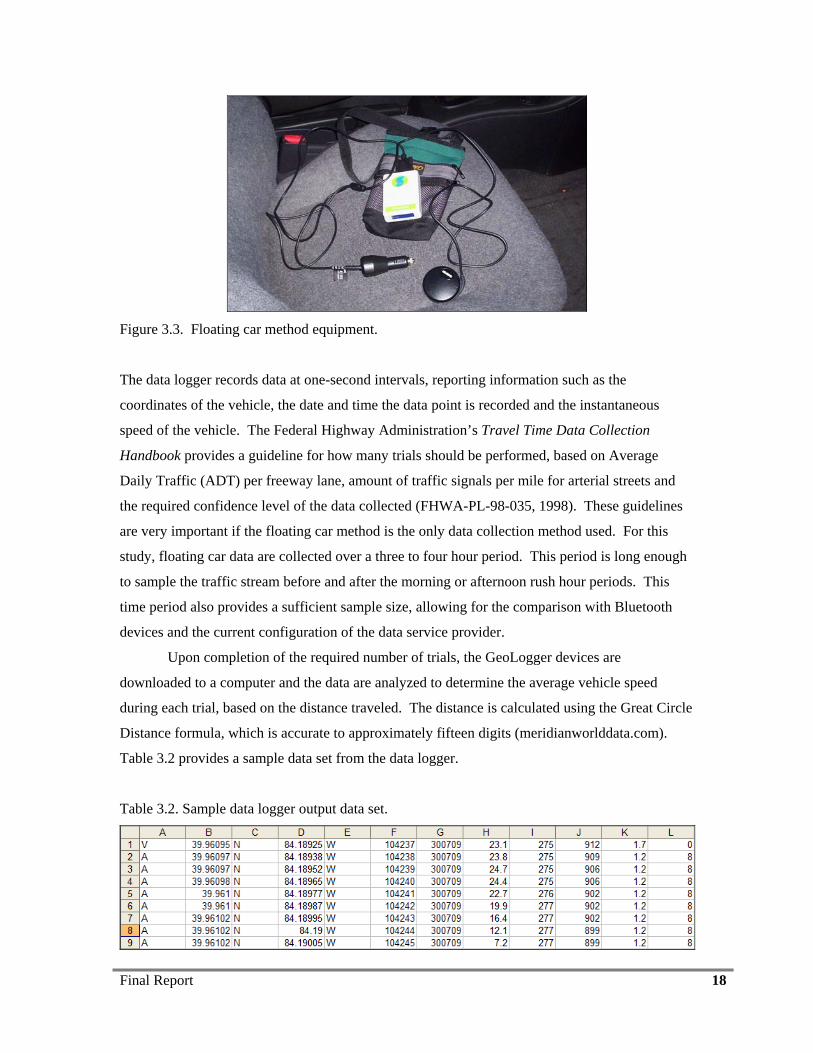
Final Report 18

Figure 3.3. Floating car method equipment.

The data logger records data at one-second intervals, reporting information such as the

coordinates of the vehicle, the date and time the data point is recorded and the instantaneous

speed of the vehicle. The Federal Highway Administration’s Travel Time Data Collection

Handbook provides a guideline for how many trials should be performed, based on Average

Daily Traffic (ADT) per freeway lane, amount of traffic signals per mile for arterial streets and

the required confidence level of the data collected (FHWA-PL-98-035, 1998). These guidelines

are very important if the floating car method is the only data collection method used. For this

study, floating car data are collected over a three to four hour period. This period is long enough

to sample the traffic stream before and after the morning or afternoon rush hour periods. This

time period also provides a sufficient sample size, allowing for the comparison with Bluetooth

devices and the current configuration of the data service provider.

Upon completion of the required number of trials, the GeoLogger devices are

downloaded to a computer and the data are analyzed to determine the average vehicle speed

during each trial, based on the distance traveled. The distance is calculated using the Great Circle

Distance formula, which is accurate to approximately fifteen digits (meridianworlddata.com).

Table 3.2 provides a sample data set from the data logger.

Table 3.2. Sample data logger output data set.

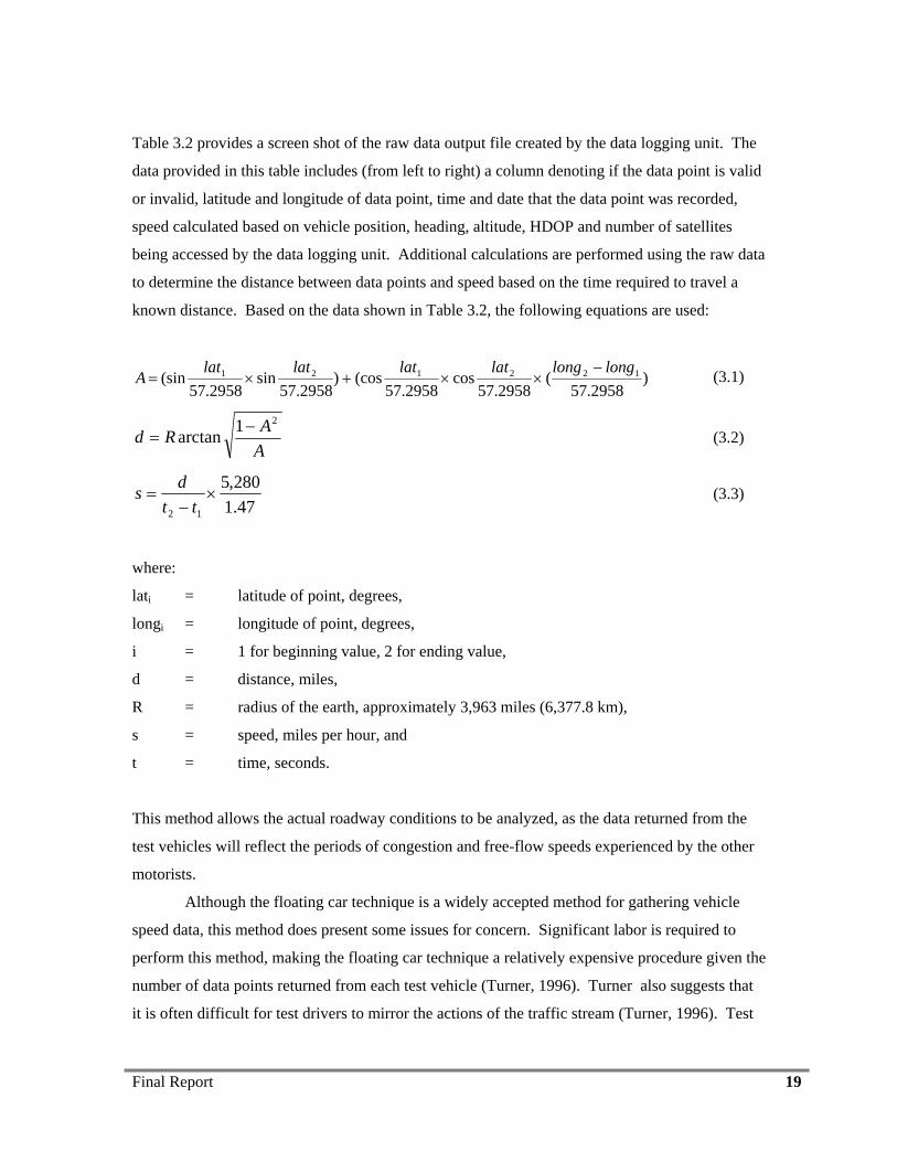
Final Report 19

Table 3.2 provides a screen shot of the raw data output file created by the data logging unit. The

data provided in this table includes (from left to right) a column denoting if the data point is valid

or invalid, latitude and longitude of data point, time and date that the data point was recorded,

speed calculated based on vehicle position, heading, altitude, HDOP and number of satellites

being accessed by the data logging unit. Additional calculations are performed using the raw data

to determine the distance between data points and speed based on the time required to travel a

known distance. Based on the data shown in Table 3.2, the following equations are used:

)2958.57

(2958.57

cos2958.57

(cos)2958.57

sin2958.57

(sin 122121 longlonglatlatlatlatA

−××+×= (3.1)

AARd

21arctan −= (3.2)

47.1280,5

12

×−

=tt

ds (3.3)

where:

lati = latitude of point, degrees,

longi = longitude of point, degrees,

i = 1 for beginning value, 2 for ending value,

d = distance, miles,

R = radius of the earth, approximately 3,963 miles (6,377.8 km),

s = speed, miles per hour, and

t = time, seconds.

This method allows the actual roadway conditions to be analyzed, as the data returned from the

test vehicles will reflect the periods of congestion and free-flow speeds experienced by the other

motorists.

Although the floating car technique is a widely accepted method for gathering vehicle

speed data, this method does present some issues for concern. Significant labor is required to

perform this method, making the floating car technique a relatively expensive procedure given the

number of data points returned from each test vehicle (Turner, 1996). Turner also suggests that

it is often difficult for test drivers to mirror the actions of the traffic stream (Turner, 1996). Test

Final Report 20

drivers often revert to their own driving habits instead of staying with the majority of traffic, or

are faced with the decision of which travel lane most closely represents the average vehicle speed.

3.4.3 Bluetooth Method

As a result of the potential limitations from the floating car, a third data collection

method using Bluetooth technology is developed to compliment the findings from the floating car

technique. In this methodology, a series of Bluetooth devices are placed at fixed locations near

the beginning and ending of the travel time segments. These devices scan the area in search of

the presence of other Bluetooth technologies, typically cell phone and headsets for cell phones.

The Bluetooth technologies send a signal back to the fixed location Bluetooth devices. This

signal contains the date and timestamp as well as the MAC address, a unique identifying number

assigned to the device. As the MAC address is unique to each device, privacy concerns will likely

arise. The MAC address of a device is assigned to the Bluetooth components when the device is

manufactured, and corresponds to the equipment only, rather than a user account (Traffax, 2008).

A second, third, or fourth Bluetooth device is placed downstream at the same time as the first and

each of these devices record the same information as previously described. The average speed of

the vehicle is based on the Bluetooth device recording the same MAC address from the upstream

and downstream device. The corresponding MAC addresses are then matched, the time required

to travel the distance between the two fixed locations is known, and based on Equation 3.4, the

average space mean speed is calculated. Equation 3.4 is shown below as:

47.15280

12

×−

=tt

ds (3.4)

where:

d = distance, miles,

s = speed, miles per hour, and

t = time, seconds.

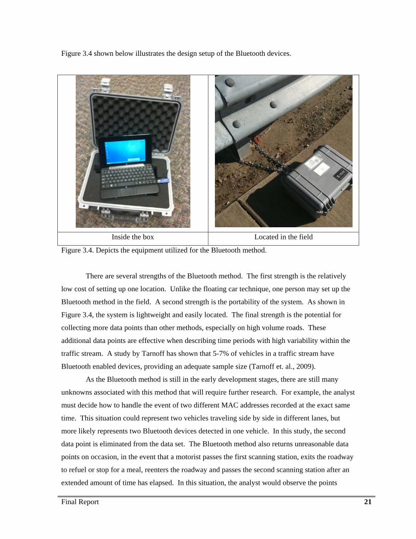
Final Report 21

Figure 3.4 shown below illustrates the design setup of the Bluetooth devices.

Inside the box Located in the field

Figure 3.4. Depicts the equipment utilized for the Bluetooth method.

There are several strengths of the Bluetooth method. The first strength is the relatively

low cost of setting up one location. Unlike the floating car technique, one person may set up the

Bluetooth method in the field. A second strength is the portability of the system. As shown in

Figure 3.4, the system is lightweight and easily located. The final strength is the potential for

collecting more data points than other methods, especially on high volume roads. These

additional data points are effective when describing time periods with high variability within the

traffic stream. A study by Tarnoff has shown that 5-7% of vehicles in a traffic stream have

Bluetooth enabled devices, providing an adequate sample size (Tarnoff et. al., 2009).

As the Bluetooth method is still in the early development stages, there are still many

unknowns associated with this method that will require further research. For example, the analyst

must decide how to handle the event of two different MAC addresses recorded at the exact same

time. This situation could represent two vehicles traveling side by side in different lanes, but

more likely represents two Bluetooth devices detected in one vehicle. In this study, the second

data point is eliminated from the data set. The Bluetooth method also returns unreasonable data

points on occasion, in the event that a motorist passes the first scanning station, exits the roadway

to refuel or stop for a meal, reenters the roadway and passes the second scanning station after an

extended amount of time has elapsed. In this situation, the analyst would observe the points

Final Report 22

recorded before and after to determine that the slow speed is an outlier, which should be

discarded.

3.5 Roadway Characteristics

The selection of the roadways used in this study is based on the travel time segments

provided by ODOT. Segment length varied, with the smallest segment measuring 0.9 miles (1.4

km) to the longest segment measuring 13.2 miles (21.2 km). These segments are located on I-70,

I-75, I-675, US-35, SR-49 and SR-4. The remaining portion of Section 3.5 describes the data

collection used with each location.

3.5.1 High Volume Access-Controlled Interstate Highways

I-70

Interstate 70 is the first interstate highway with a posted speed limit of 65 mph (104.6

km/h). Figure 3.5 depicts the beginning and ending points of the floating car trials, boxes 1 and 4,

the location of Bluetooth scanning devices and locations where spot speed readings are obtained.

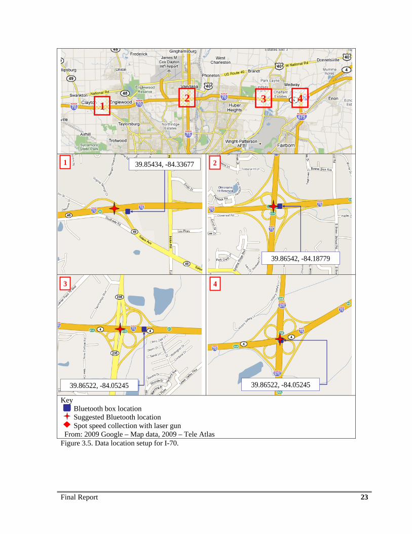
Final Report 23

142 3

39.85434, -84.336771

39.86542, -84.18779

2

39.86522, -84.05245

3

39.86522, -84.05245

4

Key Bluetooth box location Suggested Bluetooth location Spot speed collection with laser gun From: 2009 Google – Map data, 2009 – Tele Atlas Figure 3.5. Data location setup for I-70.

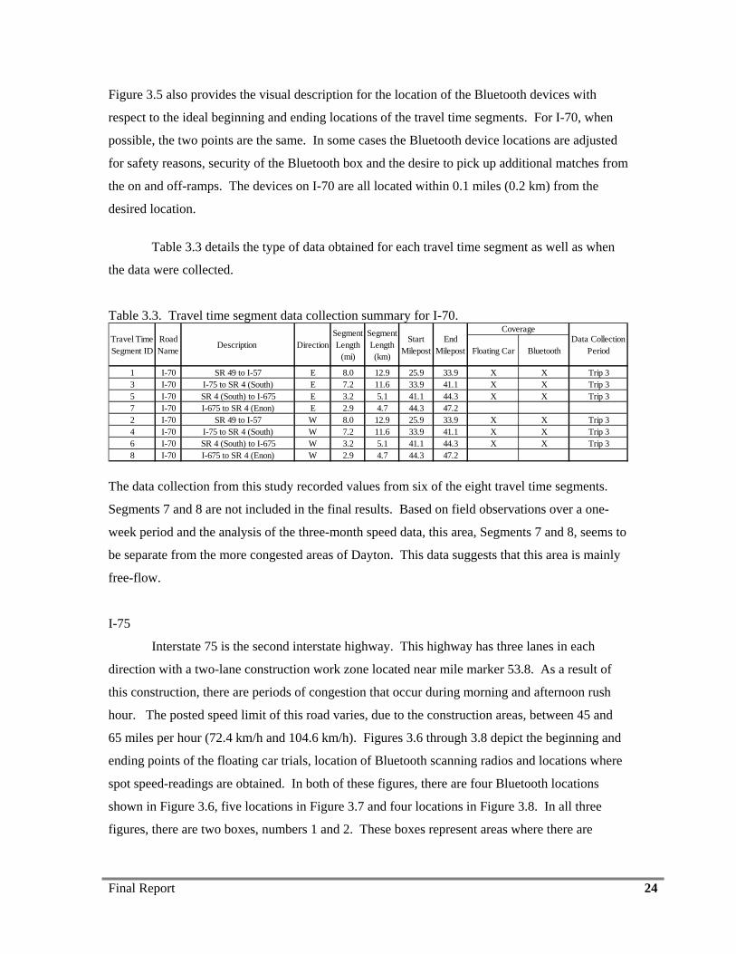
Final Report 24

Figure 3.5 also provides the visual description for the location of the Bluetooth devices with

respect to the ideal beginning and ending locations of the travel time segments. For I-70, when

possible, the two points are the same. In some cases the Bluetooth device locations are adjusted

for safety reasons, security of the Bluetooth box and the desire to pick up additional matches from

the on and off-ramps. The devices on I-70 are all located within 0.1 miles (0.2 km) from the

desired location.

Table 3.3 details the type of data obtained for each travel time segment as well as when

the data were collected.

Table 3.3. Travel time segment data collection summary for I-70.

Floating Car Bluetooth

1 I-70 SR 49 to I-57 E 8.0 12.9 25.9 33.9 X X Trip 33 I-70 I-75 to SR 4 (South) E 7.2 11.6 33.9 41.1 X X Trip 35 I-70 SR 4 (South) to I-675 E 3.2 5.1 41.1 44.3 X X Trip 37 I-70 I-675 to SR 4 (Enon) E 2.9 4.7 44.3 47.22 I-70 SR 49 to I-57 W 8.0 12.9 25.9 33.9 X X Trip 34 I-70 I-75 to SR 4 (South) W 7.2 11.6 33.9 41.1 X X Trip 36 I-70 SR 4 (South) to I-675 W 3.2 5.1 41.1 44.3 X X Trip 38 I-70 I-675 to SR 4 (Enon) W 2.9 4.7 44.3 47.2

Data CollectionPeriod

SegmentLength

(mi)

SegmentLength(km)

Travel Time Segment ID

Road Name

Description DirectionStart

MilepostEnd

Milepost

Coverage

The data collection from this study recorded values from six of the eight travel time segments.

Segments 7 and 8 are not included in the final results. Based on field observations over a one-

week period and the analysis of the three-month speed data, this area, Segments 7 and 8, seems to

be separate from the more congested areas of Dayton. This data suggests that this area is mainly

free-flow.

I-75

Interstate 75 is the second interstate highway. This highway has three lanes in each

direction with a two-lane construction work zone located near mile marker 53.8. As a result of

this construction, there are periods of congestion that occur during morning and afternoon rush

hour. The posted speed limit of this road varies, due to the construction areas, between 45 and

65 miles per hour (72.4 km/h and 104.6 km/h). Figures 3.6 through 3.8 depict the beginning and

ending points of the floating car trials, location of Bluetooth scanning radios and locations where

spot speed-readings are obtained. In both of these figures, there are four Bluetooth locations

shown in Figure 3.6, five locations in Figure 3.7 and four locations in Figure 3.8. In all three

figures, there are two boxes, numbers 1 and 2. These boxes represent areas where there are

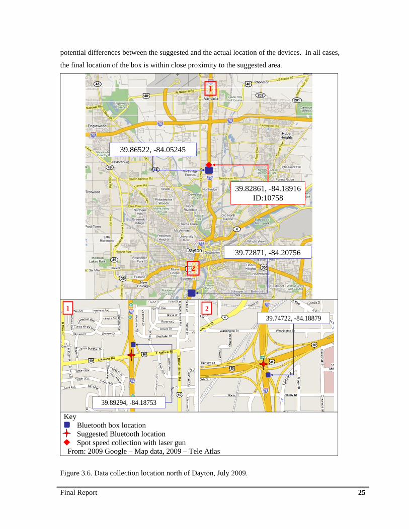
Final Report 25

potential differences between the suggested and the actual location of the devices. In all cases,

the final location of the box is within close proximity to the suggested area.

1

39.86522, -84.05245

2

39.72871, -84.20756

39.82861, -84.18916ID:10758

39.89294, -84.18753

139.74722, -84.18879

2

Key Bluetooth box location Suggested Bluetooth location Spot speed collection with laser gun From: 2009 Google – Map data, 2009 – Tele Atlas

Figure 3.6. Data collection location north of Dayton, July 2009.

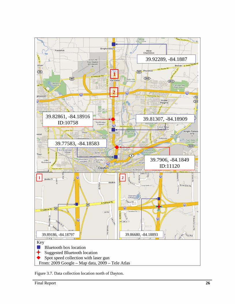
Final Report 26

1

2

39.92289, -84.1887

39.81307, -84.18909

39.77583, -84.18583

39.82861, -84.18916ID:10758

39.7906, -84.1849ID:11120

39.89186, -84.18797

1

39.86680, -84.18893

2


Figure 3.7. Data collection location north of Dayton.

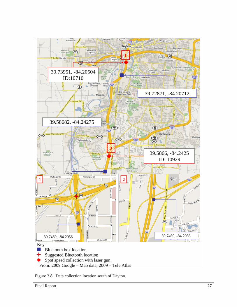
Final Report 27

1

2

39.72871, -84.20712

39.58682. -84.24275

39.5866, -84.2425 ID: 10929

39.73951, -84.20504ID:10710

39.7469, -84.2056

1

39.7469, -84.2056

2


Figure 3.8. Data collection location south of Dayton.

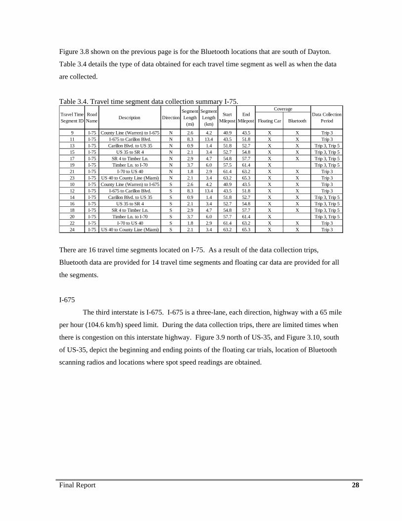
Final Report 28

Figure 3.8 shown on the previous page is for the Bluetooth locations that are south of Dayton.

Table 3.4 details the type of data obtained for each travel time segment as well as when the data

are collected.

Table 3.4. Travel time segment data collection summary I-75.


9 I-75 County Line (Warren) to I-675 N 2.6 4.2 40.9 43.5 X X Trip 311 I-75 I-675 to Carillon Blvd. N 8.3 13.4 43.5 51.8 X X Trip 313 I-75 Carillon Blvd. to US 35 N 0.9 1.4 51.8 52.7 X X Trip 3, Trip 515 I-75 US 35 to SR 4 N 2.1 3.4 52.7 54.8 X X Trip 3, Trip 517 I-75 SR 4 to Timber Ln. N 2.9 4.7 54.8 57.7 X X Trip 3, Trip 519 I-75 Timber Ln. to I-70 N 3.7 6.0 57.5 61.4 X Trip 3, Trip 521 I-75 I-70 to US 40 N 1.8 2.9 61.4 63.2 X X Trip 323 I-75 US 40 to County Line (Miami) N 2.1 3.4 63.2 65.3 X X Trip 310 I-75 County Line (Warren) to I-675 S 2.6 4.2 40.9 43.5 X X Trip 312 I-75 I-675 to Carillon Blvd. S 8.3 13.4 43.5 51.8 X X Trip 314 I-75 Carillon Blvd. to US 35 S 0.9 1.4 51.8 52.7 X X Trip 3, Trip 516 I-75 US 35 to SR 4 S 2.1 3.4 52.7 54.8 X X Trip 3, Trip 518 I-75 SR 4 to Timber Ln. S 2.9 4.7 54.8 57.7 X X Trip 3, Trip 520 I-75 Timber Ln. to I-70 S 3.7 6.0 57.7 61.4 X Trip 3, Trip 522 I-75 I-70 to US 40 S 1.8 2.9 61.4 63.2 X X Trip 324 I-75 US 40 to County Line (Miami) S 2.1 3.4 63.2 65.3 X X Trip 3


Start Milepost


Road Name

Description DirectionSegmentLength

(mi)

SegmentLength(km)

End Milepost

Coverage

There are 16 travel time segments located on I-75. As a result of the data collection trips,

Bluetooth data are provided for 14 travel time segments and floating car data are provided for all

the segments.

I-675

The third interstate is I-675. I-675 is a three-lane, each direction, highway with a 65 mile

per hour (104.6 km/h) speed limit. During the data collection trips, there are limited times when

there is congestion on this interstate highway. Figure 3.9 north of US-35, and Figure 3.10, south

of US-35, depict the beginning and ending points of the floating car trials, location of Bluetooth

scanning radios and locations where spot speed readings are obtained.

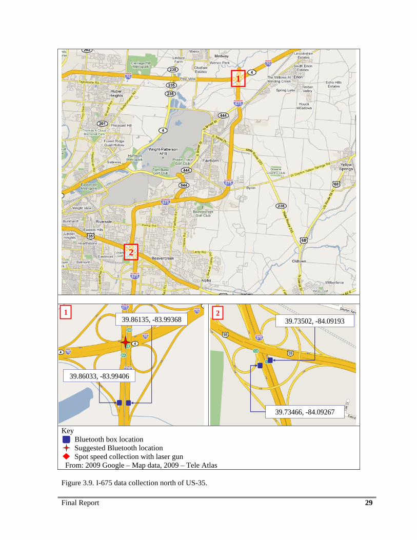
Final Report 29

1

2

39.86135, -83.99368

39.86033, -83.99406

139.73502, -84.09193

39.73466, -84.09267

2

Key Bluetooth box location Suggested Bluetooth location Spot speed collection with laser gun From: 2009 Google – Map data, 2009 – Tele Atlas Figure 3.9. I-675 data collection north of US-35.

Final Report 30

Both Bluetooth devices at location one, Figure 3.9, are approximately 0.1 miles (0.2 km)

from the suggested location as defined by ODOT. The rationale for this alternative location is to

capture vehicles travelling eastbound on I-70 merging southbound onto I-675, and vehicles

travelling northbound on I-675 merging onto I-70 eastbound. By capturing these two turning

movements, the number of Bluetooth targe radios increases, allowing for more matches. The

negative to this setup is the slight difference in the travel time segment distances and locations.

This method for capturing more vehicles by modifying the travel time segments slightly occurs

throughout this study. As shown in boxes 1 and 2 in Figures 3.9 and 3.10, there are no additional

obstructions that will significantly alter the travel times. In the final analysis, the travel times are

updated and adjusted according to the new setup.

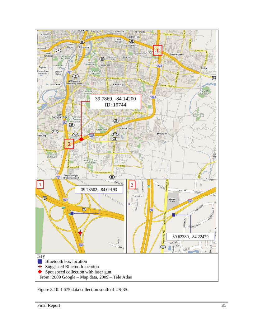
Final Report 31

1

2

39.7869, -84.14200 ID: 10744

39.73502, -84.091931

39.62389, -84.22429

2

Key Bluetooth box location Suggested Bluetooth location Spot speed collection with laser gun From: 2009 Google – Map data, 2009 – Tele Atlas Figure 3.10. I-675 data collection south of US-35.

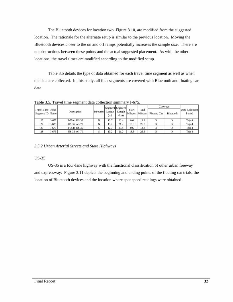
Final Report 32

The Bluetooth devices for location two, Figure 3.10, are modified from the suggested

location. The rationale for the alternate setup is similar to the previous location. Moving the

Bluetooth devices closer to the on and off ramps potentially increases the sample size. There are

no obstructions between these points and the actual suggested placement. As with the other

locations, the travel times are modified according to the modified setup.


the data are collected. In this study, all four segments are covered with Bluetooth and floating car

data.

Table 3.5. Travel time segment data collection summary I-675.


25 I-675 I-75 to US 35 N 12.7 20.4 0.6 13.3 X X Trip 427 I-675 US 35 to I-70 N 13.2 21.2 13.3 26.5 X X Trip 426 I-675 I-75 to US 35 S 12.7 20.4 0.6 13.3 X X Trip 428 I-675 US 35 to I-70 S 13.2 21.2 13.3 26.5 X X Trip 4


Start Milepost


Road Name


(mi)

SegmentLength(km)

End Milepost

Coverage

3.5.2 Urban Arterial Streets and State Highways

US-35

US-35 is a four-lane highway with the functional classification of other urban freeway

and expressway. Figure 3.11 depicts the beginning and ending points of the floating car trials, the

location of Bluetooth devices and the location where spot speed readings were obtained.

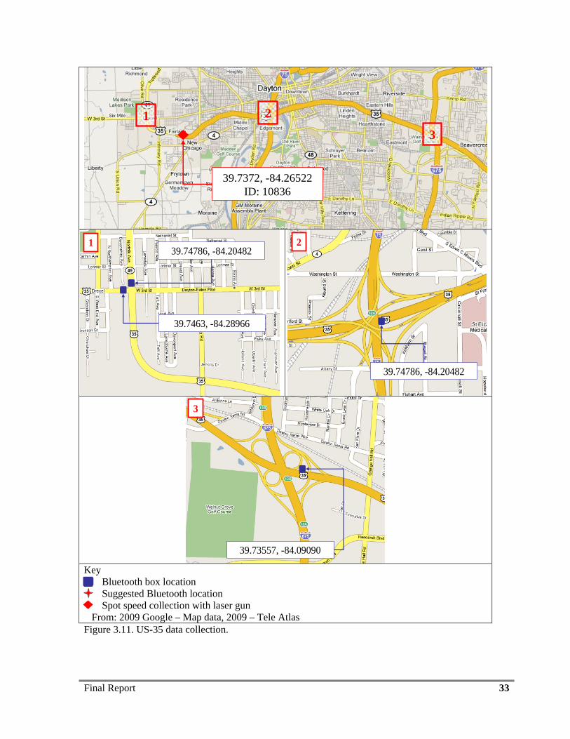
Final Report 33

213

39.7372, -84.26522 ID: 10836

39.74786, -84.204821

39.7463, -84.28966

39.74786, -84.20482

2

39.73557, -84.09090

3

Key Bluetooth box location Suggested Bluetooth location Spot speed collection with laser gun From: 2009 Google – Map data, 2009 – Tele Atlas Figure 3.11. US-35 data collection.

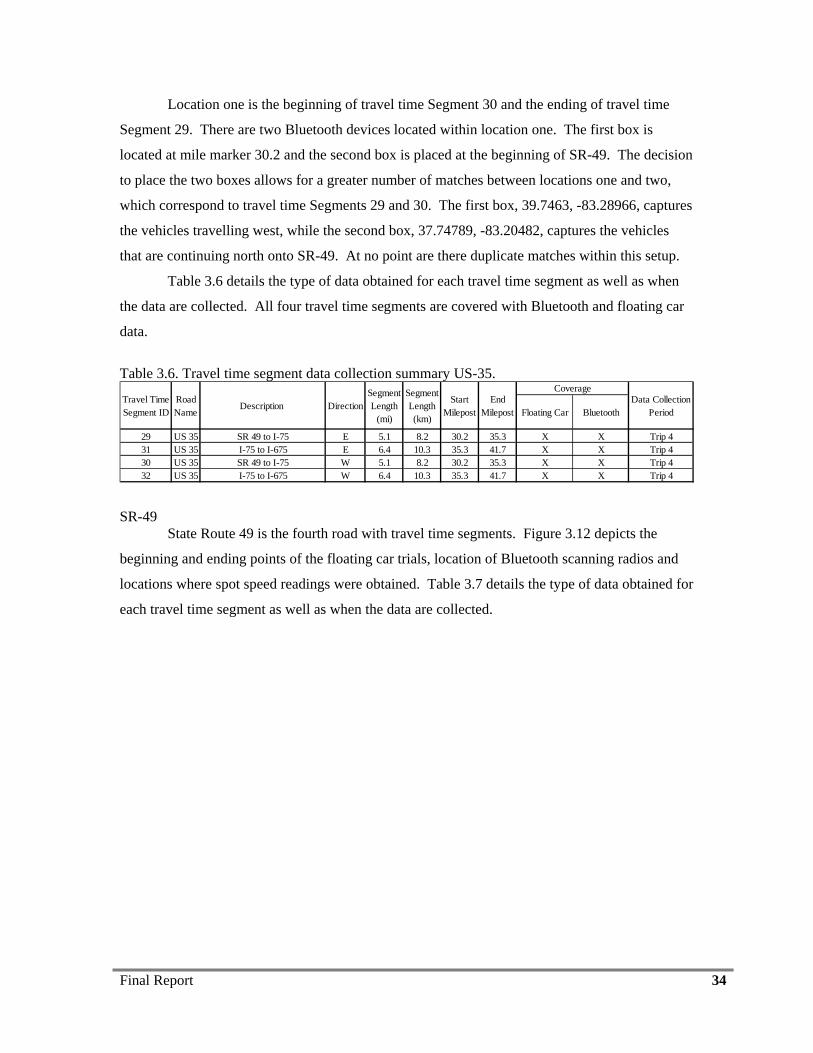
Final Report 34

Location one is the beginning of travel time Segment 30 and the ending of travel time

Segment 29. There are two Bluetooth devices located within location one. The first box is

located at mile marker 30.2 and the second box is placed at the beginning of SR-49. The decision

to place the two boxes allows for a greater number of matches between locations one and two,

which correspond to travel time Segments 29 and 30. The first box, 39.7463, -83.28966, captures

the vehicles travelling west, while the second box, 37.74789, -83.20482, captures the vehicles

that are continuing north onto SR-49. At no point are there duplicate matches within this setup.


the data are collected. All four travel time segments are covered with Bluetooth and floating car

data.

Table 3.6. Travel time segment data collection summary US-35.


29 US 35 SR 49 to I-75 E 5.1 8.2 30.2 35.3 X X Trip 431 US 35 I-75 to I-675 E 6.4 10.3 35.3 41.7 X X Trip 430 US 35 SR 49 to I-75 W 5.1 8.2 30.2 35.3 X X Trip 432 US 35 I-75 to I-675 W 6.4 10.3 35.3 41.7 X X Trip 4


Start Milepost


Road Name


(mi)

SegmentLength(km)

End Milepost

Coverage

SR-49 State Route 49 is the fourth road with travel time segments. Figure 3.12 depicts the

beginning and ending points of the floating car trials, location of Bluetooth scanning radios and

locations where spot speed readings were obtained. Table 3.7 details the type of data obtained for

each travel time segment as well as when the data are collected.

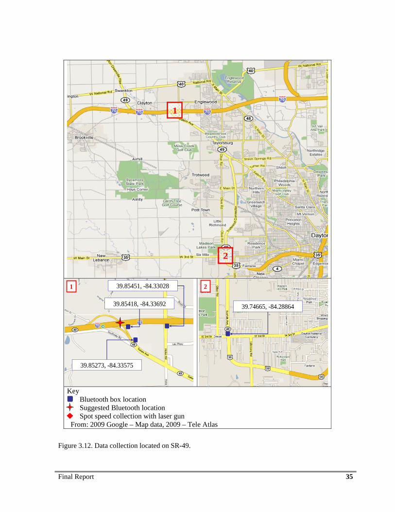
Final Report 35

1

2

39.85273, -84.33575

1

39.85418, -84.33692

39.85451, -84.33028

39.74665, -84.28864

2


Figure 3.12. Data collection located on SR-49.

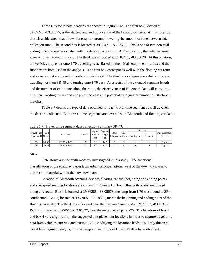
Final Report 36

Three Bluetooth box locations are shown in Figure 3.12. The first box, located at

39.85273, -83.33575, is the starting and ending location of the floating car runs. At this location,

there is a side street that allows for easy turnaround, lowering the amount of time between data

collection runs. The second box is located at 39.85471, -83.33692. This is one of two potential

ending mile markers associated with the data collection run. At this location, the vehicles must

enter onto I-70 travelling west. The third box is located at 39.85451, -83.33028. At this location,

the vehicles may enter onto I-70 travelling east. Based on the initial setup, the third box and the

first box are both used in the analysis. The first box corresponds well with the floating car route

and vehicles that are traveling north onto I-70 west. The third box captures the vehicles that are

traveling north on SR-49 and turning onto I-70 east. As a result of the extended segment length

and the number of exit points along the route, the effectiveness of Bluetooth data will come into

question. Adding the second end point increases the potential for a greater number of Bluetooth

matches.


the data are collected. Both travel time segments are covered with Bluetooth and floating car data.

Table 3.7. Travel time segment data collection summary SR-49.


35 SR 49 US 35 to I-70 N 9.0 14.5 0 9 X X Trip 436 SR 49 US 35 to I-70 S 9.0 14.5 0 9 X X Trip 4


Start Milepost


Road Name


(mi)

SegmentLength(km)

End Milepost

Coverage

SR-4

State Route 4 is the sixth roadway investigated in this study. The functional

classification of the roadway varies from urban principal arterial west of the downtown area to

urban minor arterial within the downtown area.

Location of Bluetooth scanning devices, floating car trial beginning and ending points

and spot speed reading locations are shown in Figure 3.13. Four Bluetooth boxes are located

along this route. Box 1 is located at 39.86288, -83.05673, the ramp from I-70 westbound to SR-4

southbound. Box 2, located at 39.77097, -83.18307, marks the beginning and ending point of the

floating car trials. The third box is located near the Keowee Street exit at 39.77053, -83.18315.

Box 4 is located at 39.86076, -83.05637, near the entrance ramp to I-70. The locations of box 1

and box 4 vary slightly from the suggested box placement locations in order to capture travel time

data from vehicles entering and exiting I-70. Modifying the locations leads to slightly different

travel time segment lengths, but this setup allows for more Bluetooth data to be obtained,

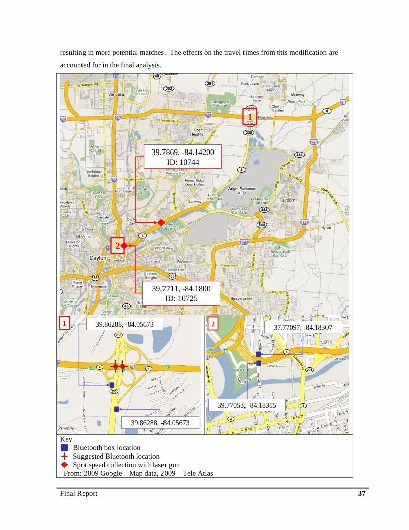
Final Report 37

resulting in more potential matches. The effects on the travel times from this modification are

accounted for in the final analysis.

1

2

39.7869, -84.14200 ID: 10744

39.7711, -84.1800 ID: 10725

39.86288, -84.056731

39.86288, -84.05673

37.77097, -84.183072

39.77053, -84.18315


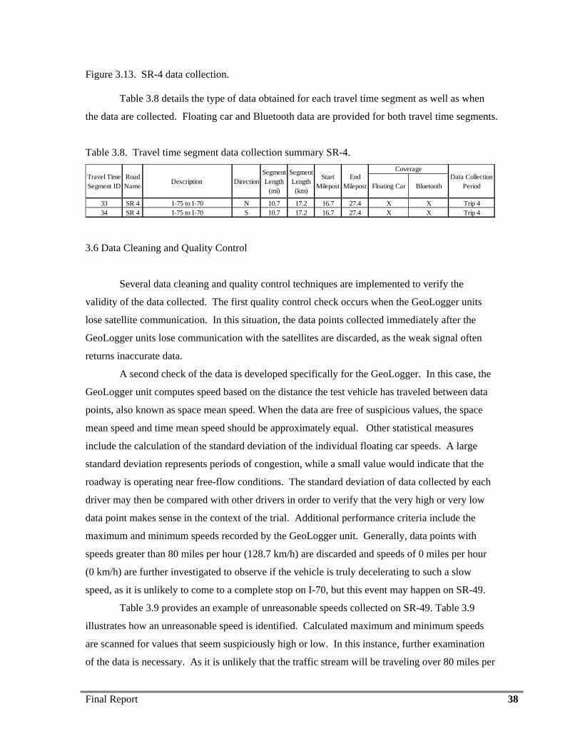
Final Report 38

Figure 3.13. SR-4 data collection.


the data are collected. Floating car and Bluetooth data are provided for both travel time segments.

Table 3.8. Travel time segment data collection summary SR-4.


33 SR 4 I-75 to I-70 N 10.7 17.2 16.7 27.4 X X Trip 434 SR 4 I-75 to I-70 S 10.7 17.2 16.7 27.4 X X Trip 4


Start Milepost


Road Name


(mi)

SegmentLength(km)

End Milepost

Coverage

3.6 Data Cleaning and Quality Control

Several data cleaning and quality control techniques are implemented to verify the

validity of the data collected. The first quality control check occurs when the GeoLogger units

lose satellite communication. In this situation, the data points collected immediately after the

GeoLogger units lose communication with the satellites are discarded, as the weak signal often

returns inaccurate data.

A second check of the data is developed specifically for the GeoLogger. In this case, the

GeoLogger unit computes speed based on the distance the test vehicle has traveled between data

points, also known as space mean speed. When the data are free of suspicious values, the space

mean speed and time mean speed should be approximately equal. Other statistical measures

include the calculation of the standard deviation of the individual floating car speeds. A large

standard deviation represents periods of congestion, while a small value would indicate that the

roadway is operating near free-flow conditions. The standard deviation of data collected by each

driver may then be compared with other drivers in order to verify that the very high or very low

data point makes sense in the context of the trial. Additional performance criteria include the

maximum and minimum speeds recorded by the GeoLogger unit. Generally, data points with

speeds greater than 80 miles per hour (128.7 km/h) are discarded and speeds of 0 miles per hour

(0 km/h) are further investigated to observe if the vehicle is truly decelerating to such a slow

speed, as it is unlikely to come to a complete stop on I-70, but this event may happen on SR-49.

Table 3.9 provides an example of unreasonable speeds collected on SR-49. Table 3.9

illustrates how an unreasonable speed is identified. Calculated maximum and minimum speeds

are scanned for values that seem suspiciously high or low. In this instance, further examination

of the data is necessary. As it is unlikely that the traffic stream will be traveling over 80 miles per

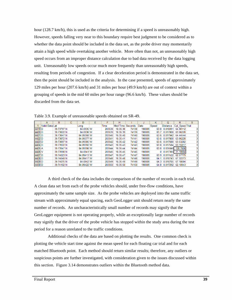
Final Report 39

hour (128.7 km/h), this is used as the criteria for determining if a speed is unreasonably high.

However, speeds falling very near to this boundary require best judgment to be considered as to

whether the data point should be included in the data set, as the probe driver may momentarily

attain a high speed while overtaking another vehicle. More often than not, an unreasonably high

speed occurs from an improper distance calculation due to bad data received by the data logging

unit. Unreasonably low speeds occur much more frequently than unreasonably high speeds,

resulting from periods of congestion. If a clear deceleration period is demonstrated in the data set,

then the point should be included in the analysis. In the case presented, speeds of approximately

129 miles per hour (207.6 km/h) and 31 miles per hour (49.9 km/h) are out of context within a

grouping of speeds in the mid 60 miles per hour range (96.6 km/h). These values should be

discarded from the data set.

Table 3.9. Example of unreasonable speeds obtained on SR-49.

A third check of the data includes the comparison of the number of records in each trial.

A clean data set from each of the probe vehicles should, under free-flow conditions, have

approximately the same sample size. As the probe vehicles are deployed into the same traffic

stream with approximately equal spacing, each GeoLogger unit should return nearly the same

number of records. An uncharacteristically small number of records may signify that the

GeoLogger equipment is not operating properly, while an exceptionally large number of records

may signify that the driver of the probe vehicle has stopped within the study area during the test

period for a reason unrelated to the traffic conditions.

Additional checks of the data are based on plotting the results. One common check is

plotting the vehicle start time against the mean speed for each floating car trial and for each

matched Bluetooth point. Each method should return similar results; therefore, any outliers or

suspicious points are further investigated, with consideration given to the issues discussed within

this section. Figure 3.14 demonstrates outliers within the Bluetooth method data.

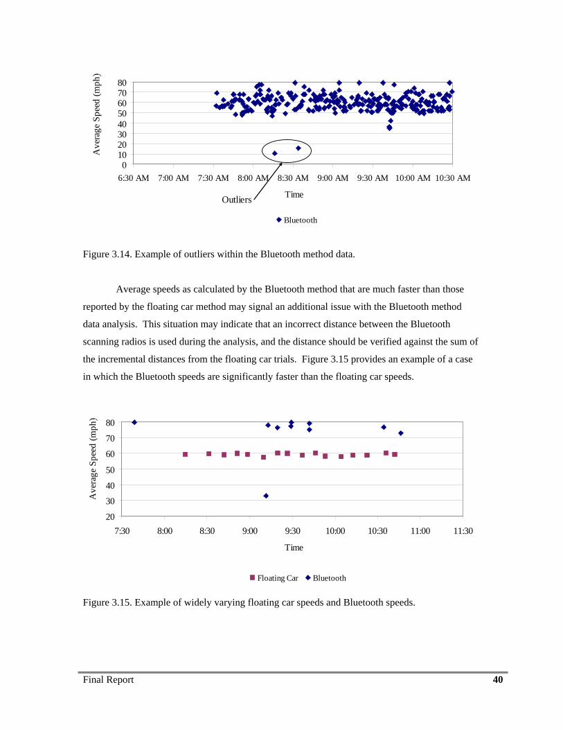
Final Report 40

01020304050607080

6:30 AM 7:00 AM 7:30 AM 8:00 AM 8:30 AM 9:00 AM 9:30 AM 10:00 AM 10:30 AM

Time

Ave

rage

Spe

ed (m

ph).

Bluetooth

Outliers

Figure 3.14. Example of outliers within the Bluetooth method data.

Average speeds as calculated by the Bluetooth method that are much faster than those

reported by the floating car method may signal an additional issue with the Bluetooth method

data analysis. This situation may indicate that an incorrect distance between the Bluetooth

scanning radios is used during the analysis, and the distance should be verified against the sum of

the incremental distances from the floating car trials. Figure 3.15 provides an example of a case

in which the Bluetooth speeds are significantly faster than the floating car speeds.

20

30

40

50

60

70

80

7:30 8:00 8:30 9:00 9:30 10:00 10:30 11:00 11:30

Time

Ave

rage

Spe

ed (m

ph).


Figure 3.15. Example of widely varying floating car speeds and Bluetooth speeds.

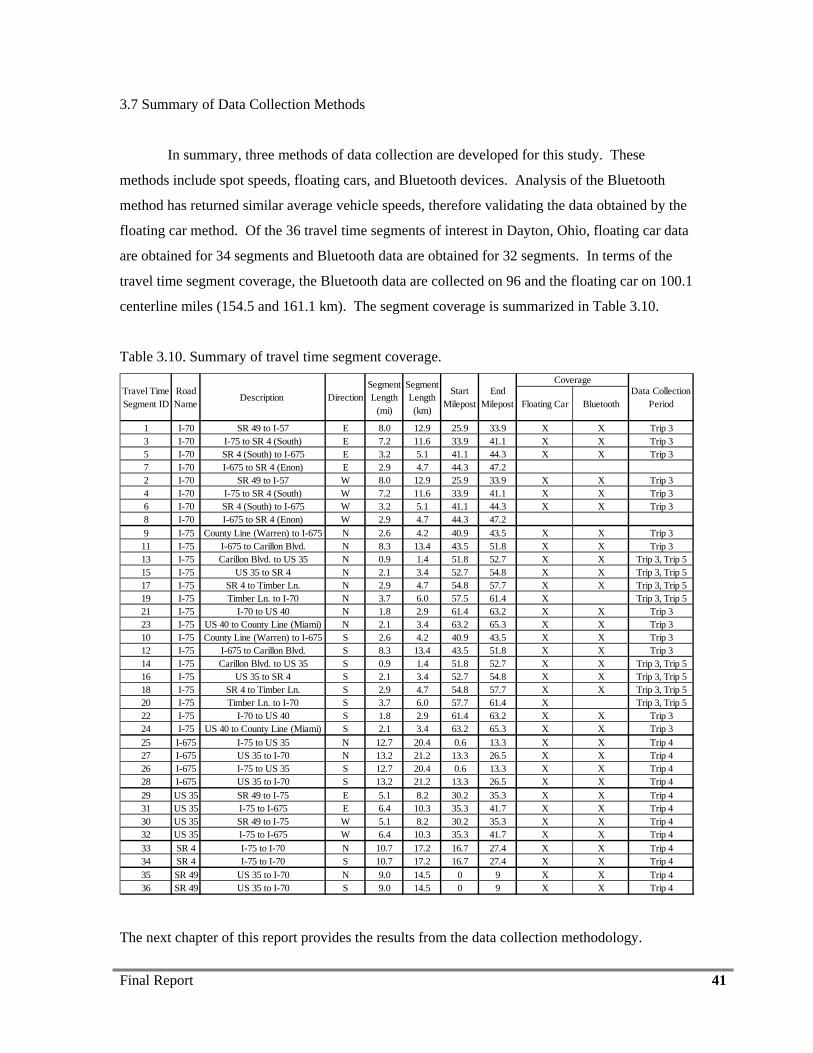
Final Report 41

3.7 Summary of Data Collection Methods

In summary, three methods of data collection are developed for this study. These

methods include spot speeds, floating cars, and Bluetooth devices. Analysis of the Bluetooth

method has returned similar average vehicle speeds, therefore validating the data obtained by the

floating car method. Of the 36 travel time segments of interest in Dayton, Ohio, floating car data

are obtained for 34 segments and Bluetooth data are obtained for 32 segments. In terms of the

travel time segment coverage, the Bluetooth data are collected on 96 and the floating car on 100.1

centerline miles (154.5 and 161.1 km). The segment coverage is summarized in Table 3.10.

Table 3.10. Summary of travel time segment coverage.


1 I-70 SR 49 to I-57 E 8.0 12.9 25.9 33.9 X X Trip 33 I-70 I-75 to SR 4 (South) E 7.2 11.6 33.9 41.1 X X Trip 35 I-70 SR 4 (South) to I-675 E 3.2 5.1 41.1 44.3 X X Trip 37 I-70 I-675 to SR 4 (Enon) E 2.9 4.7 44.3 47.22 I-70 SR 49 to I-57 W 8.0 12.9 25.9 33.9 X X Trip 34 I-70 I-75 to SR 4 (South) W 7.2 11.6 33.9 41.1 X X Trip 36 I-70 SR 4 (South) to I-675 W 3.2 5.1 41.1 44.3 X X Trip 38 I-70 I-675 to SR 4 (Enon) W 2.9 4.7 44.3 47.29 I-75 County Line (Warren) to I-675 N 2.6 4.2 40.9 43.5 X X Trip 3

11 I-75 I-675 to Carillon Blvd. N 8.3 13.4 43.5 51.8 X X Trip 313 I-75 Carillon Blvd. to US 35 N 0.9 1.4 51.8 52.7 X X Trip 3, Trip 515 I-75 US 35 to SR 4 N 2.1 3.4 52.7 54.8 X X Trip 3, Trip 517 I-75 SR 4 to Timber Ln. N 2.9 4.7 54.8 57.7 X X Trip 3, Trip 519 I-75 Timber Ln. to I-70 N 3.7 6.0 57.5 61.4 X Trip 3, Trip 521 I-75 I-70 to US 40 N 1.8 2.9 61.4 63.2 X X Trip 323 I-75 US 40 to County Line (Miami) N 2.1 3.4 63.2 65.3 X X Trip 310 I-75 County Line (Warren) to I-675 S 2.6 4.2 40.9 43.5 X X Trip 312 I-75 I-675 to Carillon Blvd. S 8.3 13.4 43.5 51.8 X X Trip 314 I-75 Carillon Blvd. to US 35 S 0.9 1.4 51.8 52.7 X X Trip 3, Trip 516 I-75 US 35 to SR 4 S 2.1 3.4 52.7 54.8 X X Trip 3, Trip 518 I-75 SR 4 to Timber Ln. S 2.9 4.7 54.8 57.7 X X Trip 3, Trip 520 I-75 Timber Ln. to I-70 S 3.7 6.0 57.7 61.4 X Trip 3, Trip 522 I-75 I-70 to US 40 S 1.8 2.9 61.4 63.2 X X Trip 324 I-75 US 40 to County Line (Miami) S 2.1 3.4 63.2 65.3 X X Trip 325 I-675 I-75 to US 35 N 12.7 20.4 0.6 13.3 X X Trip 427 I-675 US 35 to I-70 N 13.2 21.2 13.3 26.5 X X Trip 426 I-675 I-75 to US 35 S 12.7 20.4 0.6 13.3 X X Trip 428 I-675 US 35 to I-70 S 13.2 21.2 13.3 26.5 X X Trip 429 US 35 SR 49 to I-75 E 5.1 8.2 30.2 35.3 X X Trip 431 US 35 I-75 to I-675 E 6.4 10.3 35.3 41.7 X X Trip 430 US 35 SR 49 to I-75 W 5.1 8.2 30.2 35.3 X X Trip 432 US 35 I-75 to I-675 W 6.4 10.3 35.3 41.7 X X Trip 433 SR 4 I-75 to I-70 N 10.7 17.2 16.7 27.4 X X Trip 434 SR 4 I-75 to I-70 S 10.7 17.2 16.7 27.4 X X Trip 435 SR 49 US 35 to I-70 N 9.0 14.5 0 9 X X Trip 436 SR 49 US 35 to I-70 S 9.0 14.5 0 9 X X Trip 4


End Milepost

Start Milepost


Coverage

DirectionDescription Road Name

SegmentLength

(mi)

SegmentLength(km)

The next chapter of this report provides the results from the data collection methodology.

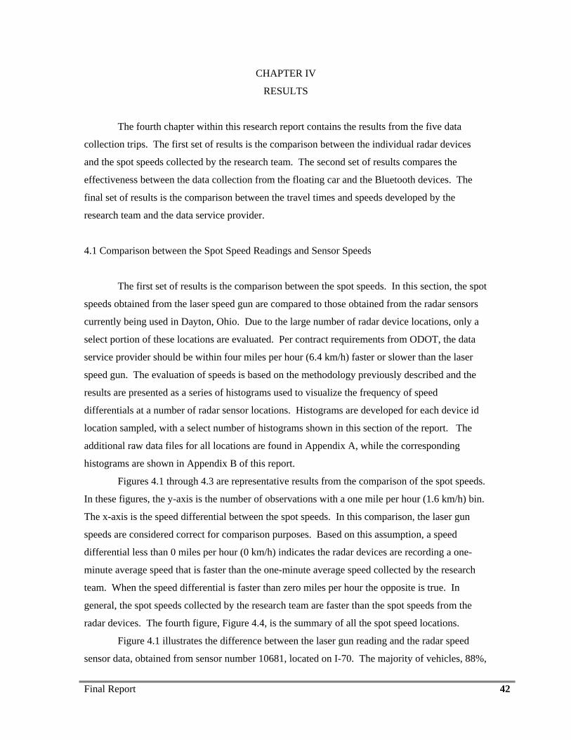
Final Report 42

CHAPTER IV

RESULTS

The fourth chapter within this research report contains the results from the five data

collection trips. The first set of results is the comparison between the individual radar devices

and the spot speeds collected by the research team. The second set of results compares the

effectiveness between the data collection from the floating car and the Bluetooth devices. The

final set of results is the comparison between the travel times and speeds developed by the

research team and the data service provider.

4.1 Comparison between the Spot Speed Readings and Sensor Speeds

The first set of results is the comparison between the spot speeds. In this section, the spot

speeds obtained from the laser speed gun are compared to those obtained from the radar sensors

currently being used in Dayton, Ohio. Due to the large number of radar device locations, only a

select portion of these locations are evaluated. Per contract requirements from ODOT, the data

service provider should be within four miles per hour (6.4 km/h) faster or slower than the laser

speed gun. The evaluation of speeds is based on the methodology previously described and the

results are presented as a series of histograms used to visualize the frequency of speed

differentials at a number of radar sensor locations. Histograms are developed for each device id

location sampled, with a select number of histograms shown in this section of the report. The

additional raw data files for all locations are found in Appendix A, while the corresponding

histograms are shown in Appendix B of this report.

Figures 4.1 through 4.3 are representative results from the comparison of the spot speeds.

In these figures, the y-axis is the number of observations with a one mile per hour (1.6 km/h) bin.

The x-axis is the speed differential between the spot speeds. In this comparison, the laser gun

speeds are considered correct for comparison purposes. Based on this assumption, a speed

differential less than 0 miles per hour (0 km/h) indicates the radar devices are recording a one-

minute average speed that is faster than the one-minute average speed collected by the research

team. When the speed differential is faster than zero miles per hour the opposite is true. In

general, the spot speeds collected by the research team are faster than the spot speeds from the

radar devices. The fourth figure, Figure 4.4, is the summary of all the spot speed locations.

Figure 4.1 illustrates the difference between the laser gun reading and the radar speed

sensor data, obtained from sensor number 10681, located on I-70. The majority of vehicles, 88%,

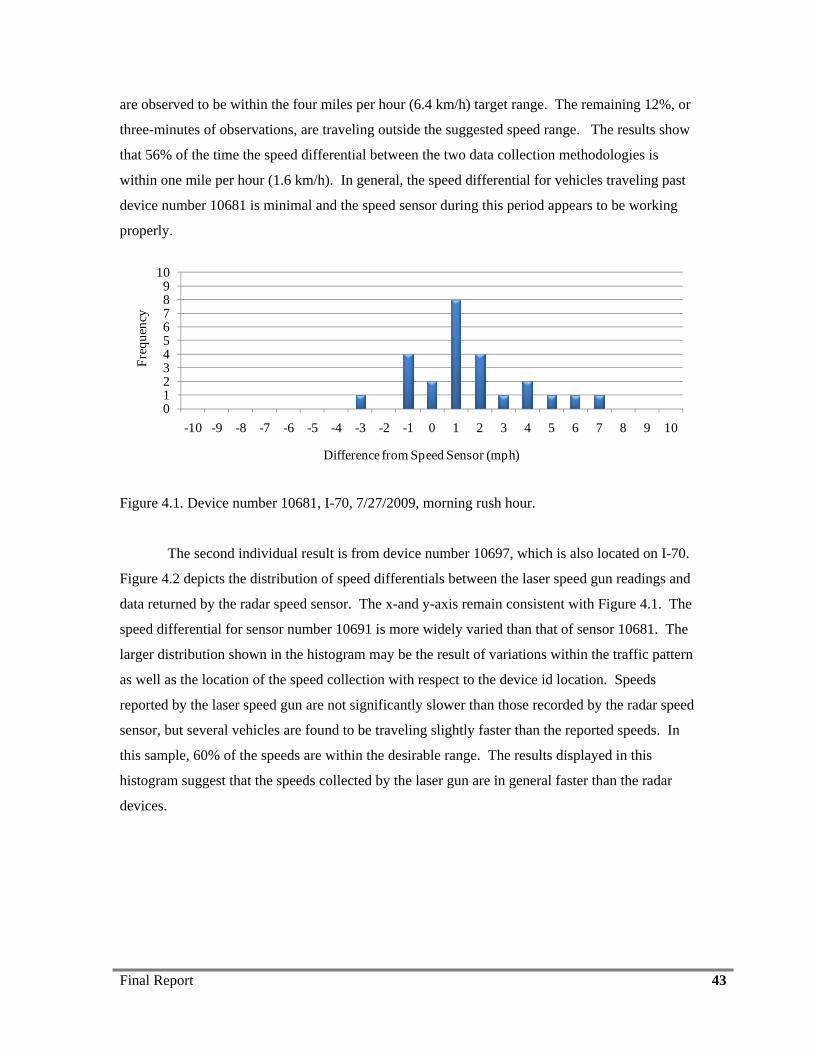
Final Report 43

are observed to be within the four miles per hour (6.4 km/h) target range. The remaining 12%, or

three-minutes of observations, are traveling outside the suggested speed range. The results show

that 56% of the time the speed differential between the two data collection methodologies is

within one mile per hour (1.6 km/h). In general, the speed differential for vehicles traveling past

device number 10681 is minimal and the speed sensor during this period appears to be working

properly.

0123456789

10

-10 -9 -8 -7 -6 -5 -4 -3 -2 -1 0 1 2 3 4 5 6 7 8 9 10

Freq

uenc

y

Difference from Speed Sensor (mph)

Figure 4.1. Device number 10681, I-70, 7/27/2009, morning rush hour.

The second individual result is from device number 10697, which is also located on I-70.

Figure 4.2 depicts the distribution of speed differentials between the laser speed gun readings and

data returned by the radar speed sensor. The x-and y-axis remain consistent with Figure 4.1. The

speed differential for sensor number 10691 is more widely varied than that of sensor 10681. The

larger distribution shown in the histogram may be the result of variations within the traffic pattern

as well as the location of the speed collection with respect to the device id location. Speeds

reported by the laser speed gun are not significantly slower than those recorded by the radar speed

sensor, but several vehicles are found to be traveling slightly faster than the reported speeds. In

this sample, 60% of the speeds are within the desirable range. The results displayed in this

histogram suggest that the speeds collected by the laser gun are in general faster than the radar

devices.

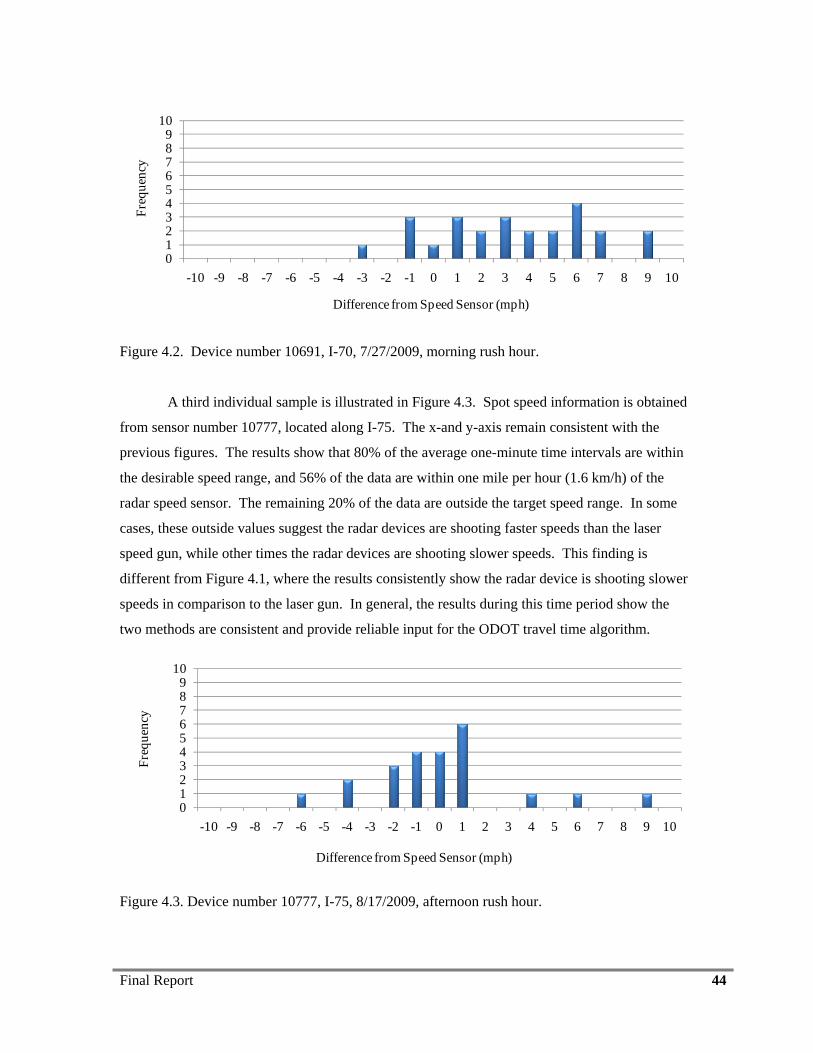
Final Report 44

0123456789

10

-10 -9 -8 -7 -6 -5 -4 -3 -2 -1 0 1 2 3 4 5 6 7 8 9 10

Freq

uenc

y


Figure 4.2. Device number 10691, I-70, 7/27/2009, morning rush hour.

A third individual sample is illustrated in Figure 4.3. Spot speed information is obtained

from sensor number 10777, located along I-75. The x-and y-axis remain consistent with the

previous figures. The results show that 80% of the average one-minute time intervals are within

the desirable speed range, and 56% of the data are within one mile per hour (1.6 km/h) of the

radar speed sensor. The remaining 20% of the data are outside the target speed range. In some

cases, these outside values suggest the radar devices are shooting faster speeds than the laser

speed gun, while other times the radar devices are shooting slower speeds. This finding is

different from Figure 4.1, where the results consistently show the radar device is shooting slower

speeds in comparison to the laser gun. In general, the results during this time period show the

two methods are consistent and provide reliable input for the ODOT travel time algorithm.

0123456789

10

-10 -9 -8 -7 -6 -5 -4 -3 -2 -1 0 1 2 3 4 5 6 7 8 9 10

Freq

uenc

y


Figure 4.3. Device number 10777, I-75, 8/17/2009, afternoon rush hour.

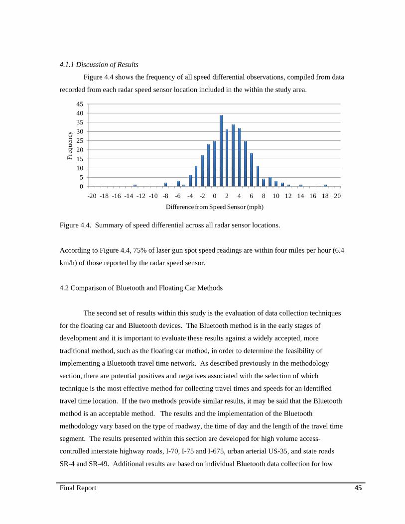
Final Report 45

4.1.1 Discussion of Results

Figure 4.4 shows the frequency of all speed differential observations, compiled from data

recorded from each radar speed sensor location included in the within the study area.

05

1015202530354045

-20 -18 -16 -14 -12 -10 -8 -6 -4 -2 0 2 4 6 8 10 12 14 16 18 20

Freq

uenc

y


Figure 4.4. Summary of speed differential across all radar sensor locations.

According to Figure 4.4, 75% of laser gun spot speed readings are within four miles per hour (6.4

km/h) of those reported by the radar speed sensor.

4.2 Comparison of Bluetooth and Floating Car Methods

The second set of results within this study is the evaluation of data collection techniques

for the floating car and Bluetooth devices. The Bluetooth method is in the early stages of

development and it is important to evaluate these results against a widely accepted, more

traditional method, such as the floating car method, in order to determine the feasibility of

implementing a Bluetooth travel time network. As described previously in the methodology

section, there are potential positives and negatives associated with the selection of which

technique is the most effective method for collecting travel times and speeds for an identified

travel time location. If the two methods provide similar results, it may be said that the Bluetooth

method is an acceptable method. The results and the implementation of the Bluetooth

methodology vary based on the type of roadway, the time of day and the length of the travel time

segment. The results presented within this section are developed for high volume access-

controlled interstate highway roads, I-70, I-75 and I-675, urban arterial US-35, and state roads

SR-4 and SR-49. Additional results are based on individual Bluetooth data collection for low

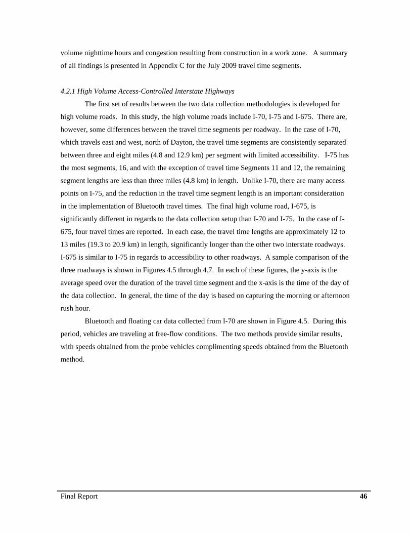
Final Report 46

volume nighttime hours and congestion resulting from construction in a work zone. A summary

of all findings is presented in Appendix C for the July 2009 travel time segments.


The first set of results between the two data collection methodologies is developed for

high volume roads. In this study, the high volume roads include I-70, I-75 and I-675. There are,

however, some differences between the travel time segments per roadway. In the case of I-70,

which travels east and west, north of Dayton, the travel time segments are consistently separated

between three and eight miles (4.8 and 12.9 km) per segment with limited accessibility. I-75 has

the most segments, 16, and with the exception of travel time Segments 11 and 12, the remaining

segment lengths are less than three miles (4.8 km) in length. Unlike I-70, there are many access

points on I-75, and the reduction in the travel time segment length is an important consideration

in the implementation of Bluetooth travel times. The final high volume road, I-675, is

significantly different in regards to the data collection setup than I-70 and I-75. In the case of I-

675, four travel times are reported. In each case, the travel time lengths are approximately 12 to

13 miles (19.3 to 20.9 km) in length, significantly longer than the other two interstate roadways.

I-675 is similar to I-75 in regards to accessibility to other roadways. A sample comparison of the

three roadways is shown in Figures 4.5 through 4.7. In each of these figures, the y-axis is the

average speed over the duration of the travel time segment and the x-axis is the time of the day of

the data collection. In general, the time of the day is based on capturing the morning or afternoon

rush hour.

Bluetooth and floating car data collected from I-70 are shown in Figure 4.5. During this

period, vehicles are traveling at free-flow conditions. The two methods provide similar results,

with speeds obtained from the probe vehicles complimenting speeds obtained from the Bluetooth

method.

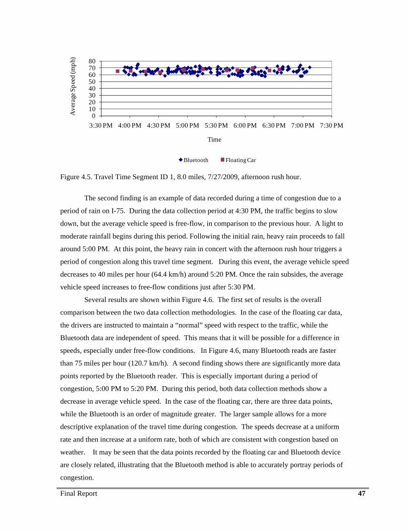
Final Report 47

01020304050607080

3:30 PM 4:00 PM 4:30 PM 5:00 PM 5:30 PM 6:00 PM 6:30 PM 7:00 PM 7:30 PM

Ave

rage

Spe

ed (m

ph).

Time

Bluetooth Floating Car

Figure 4.5. Travel Time Segment ID 1, 8.0 miles, 7/27/2009, afternoon rush hour.

The second finding is an example of data recorded during a time of congestion due to a

period of rain on I-75. During the data collection period at 4:30 PM, the traffic begins to slow

down, but the average vehicle speed is free-flow, in comparison to the previous hour. A light to

moderate rainfall begins during this period. Following the initial rain, heavy rain proceeds to fall

around 5:00 PM. At this point, the heavy rain in concert with the afternoon rush hour triggers a

period of congestion along this travel time segment. During this event, the average vehicle speed

decreases to 40 miles per hour (64.4 km/h) around 5:20 PM. Once the rain subsides, the average

vehicle speed increases to free-flow conditions just after 5:30 PM.

Several results are shown within Figure 4.6. The first set of results is the overall

comparison between the two data collection methodologies. In the case of the floating car data,

the drivers are instructed to maintain a “normal” speed with respect to the traffic, while the

Bluetooth data are independent of speed. This means that it will be possible for a difference in

speeds, especially under free-flow conditions. In Figure 4.6, many Bluetooth reads are faster

than 75 miles per hour (120.7 km/h). A second finding shows there are significantly more data

points reported by the Bluetooth reader. This is especially important during a period of

congestion, 5:00 PM to 5:20 PM. During this period, both data collection methods show a

decrease in average vehicle speed. In the case of the floating car, there are three data points,

while the Bluetooth is an order of magnitude greater. The larger sample allows for a more

descriptive explanation of the travel time during congestion. The speeds decrease at a uniform

rate and then increase at a uniform rate, both of which are consistent with congestion based on

weather. It may be seen that the data points recorded by the floating car and Bluetooth device

are closely related, illustrating that the Bluetooth method is able to accurately portray periods of

congestion.

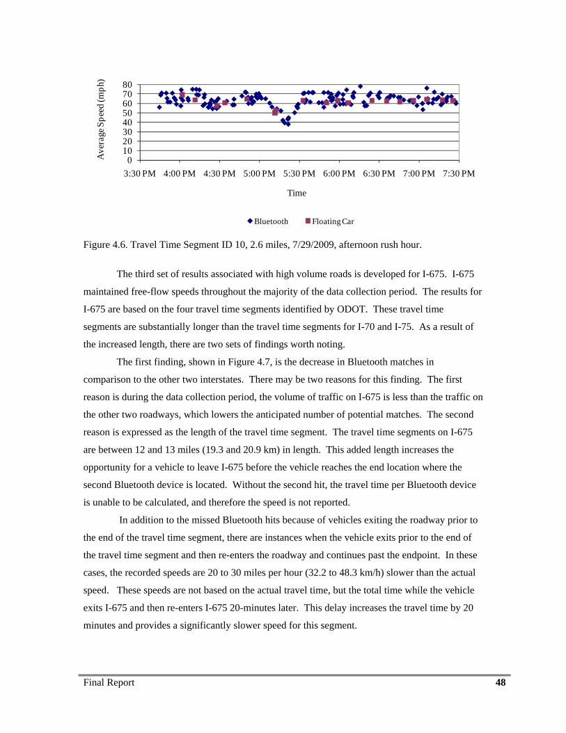
Final Report 48

01020304050607080


Ave

rage

Spe

ed (m

ph).

Time



The third set of results associated with high volume roads is developed for I-675. I-675

maintained free-flow speeds throughout the majority of the data collection period. The results for

I-675 are based on the four travel time segments identified by ODOT. These travel time

segments are substantially longer than the travel time segments for I-70 and I-75. As a result of

the increased length, there are two sets of findings worth noting.

The first finding, shown in Figure 4.7, is the decrease in Bluetooth matches in

comparison to the other two interstates. There may be two reasons for this finding. The first

reason is during the data collection period, the volume of traffic on I-675 is less than the traffic on

the other two roadways, which lowers the anticipated number of potential matches. The second

reason is expressed as the length of the travel time segment. The travel time segments on I-675

are between 12 and 13 miles (19.3 and 20.9 km) in length. This added length increases the

opportunity for a vehicle to leave I-675 before the vehicle reaches the end location where the

second Bluetooth device is located. Without the second hit, the travel time per Bluetooth device

is unable to be calculated, and therefore the speed is not reported.

In addition to the missed Bluetooth hits because of vehicles exiting the roadway prior to

the end of the travel time segment, there are instances when the vehicle exits prior to the end of

the travel time segment and then re-enters the roadway and continues past the endpoint. In these

cases, the recorded speeds are 20 to 30 miles per hour (32.2 to 48.3 km/h) slower than the actual

speed. These speeds are not based on the actual travel time, but the total time while the vehicle

exits I-675 and then re-enters I-675 20-minutes later. This delay increases the travel time by 20

minutes and provides a significantly slower speed for this segment.

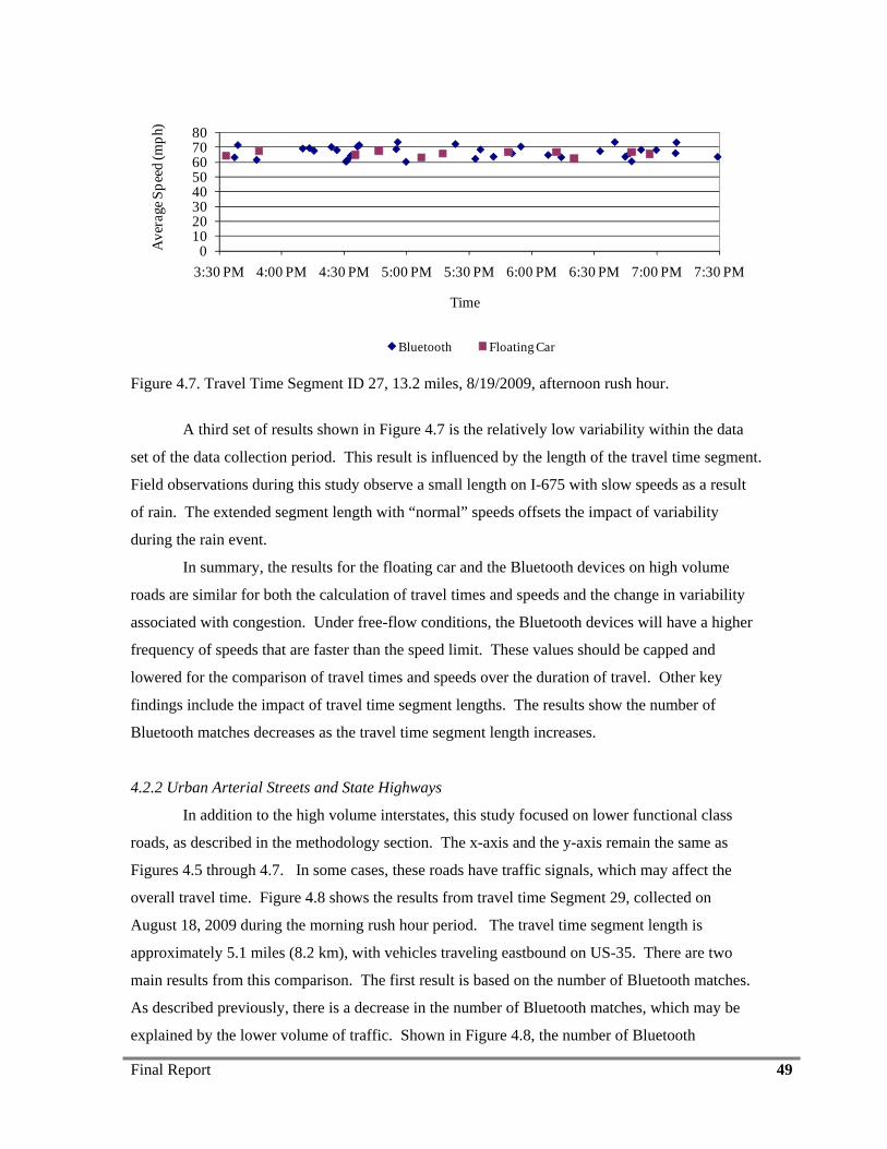
Final Report 49

01020304050607080


Ave

rage

Spe

ed (m

ph).

Time



A third set of results shown in Figure 4.7 is the relatively low variability within the data

set of the data collection period. This result is influenced by the length of the travel time segment.

Field observations during this study observe a small length on I-675 with slow speeds as a result

of rain. The extended segment length with “normal” speeds offsets the impact of variability

during the rain event.

In summary, the results for the floating car and the Bluetooth devices on high volume

roads are similar for both the calculation of travel times and speeds and the change in variability

associated with congestion. Under free-flow conditions, the Bluetooth devices will have a higher

frequency of speeds that are faster than the speed limit. These values should be capped and

lowered for the comparison of travel times and speeds over the duration of travel. Other key

findings include the impact of travel time segment lengths. The results show the number of

Bluetooth matches decreases as the travel time segment length increases.

4.2.2 Urban Arterial Streets and State Highways

In addition to the high volume interstates, this study focused on lower functional class

roads, as described in the methodology section. The x-axis and the y-axis remain the same as

Figures 4.5 through 4.7. In some cases, these roads have traffic signals, which may affect the

overall travel time. Figure 4.8 shows the results from travel time Segment 29, collected on

August 18, 2009 during the morning rush hour period. The travel time segment length is

approximately 5.1 miles (8.2 km), with vehicles traveling eastbound on US-35. There are two

main results from this comparison. The first result is based on the number of Bluetooth matches.

As described previously, there is a decrease in the number of Bluetooth matches, which may be

explained by the lower volume of traffic. Shown in Figure 4.8, the number of Bluetooth

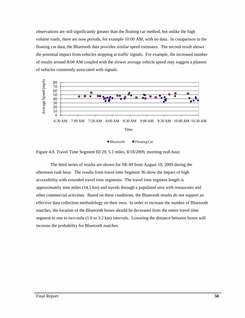
Final Report 50

observations are still significantly greater than the floating car method, but unlike the high

volume roads, there are now periods, for example 10:00 AM, with no data. In comparison to the

floating car data, the Bluetooth data provides similar speed estimates. The second result shows

the potential impact from vehicles stopping at traffic signals. For example, the increased number

of results around 8:00 AM coupled with the slower average vehicle speed may suggest a platoon

of vehicles commonly associated with signals.

01020304050607080


Ave

rage

Spe

ed (m

ph).

Time


Figure 4.8. Travel Time Segment ID 29, 5.1 miles, 8/18/2009, morning rush hour.

The third series of results are shown for SR-49 from August 18, 2009 during the

afternoon rush hour. The results from travel time Segment 36 show the impact of high

accessibility with extended travel time segments. The travel time segment length is

approximately nine miles (14.5 km) and travels through a populated area with restaurants and

other commercial activities. Based on these conditions, the Bluetooth results do not support an

effective data collection methodology on their own. In order to increase the number of Bluetooth

matches, the location of the Bluetooth boxes should be decreased from the entire travel time

segment to one to two-mile (1.6 to 3.2 km) intervals. Lowering the distance between boxes will

increase the probability for Bluetooth matches.

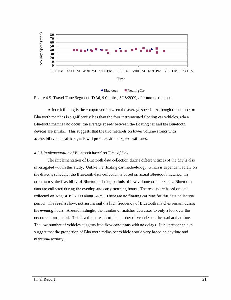
Final Report 51

01020304050607080


Ave

rage

Spe

ed (m

ph).

Time



A fourth finding is the comparison between the average speeds. Although the number of

Bluetooth matches is significantly less than the four instrumented floating car vehicles, when

Bluetooth matches do occur, the average speeds between the floating car and the Bluetooth

devices are similar. This suggests that the two methods on lower volume streets with

accessibility and traffic signals will produce similar speed estimates.

4.2.3 Implementation of Bluetooth based on Time of Day

The implementation of Bluetooth data collection during different times of the day is also

investigated within this study. Unlike the floating car methodology, which is dependant solely on

the driver’s schedule, the Bluetooth data collection is based on actual Bluetooth matches. In

order to test the feasibility of Bluetooth during periods of low volume on interstates, Bluetooth

data are collected during the evening and early morning hours. The results are based on data

collected on August 19, 2009 along I-675. There are no floating car runs for this data collection

period. The results show, not surprisingly, a high frequency of Bluetooth matches remain during

the evening hours. Around midnight, the number of matches decreases to only a few over the

next one-hour period. This is a direct result of the number of vehicles on the road at that time.

The low number of vehicles suggests free-flow conditions with no delays. It is unreasonable to

suggest that the proportion of Bluetooth radios per vehicle would vary based on daytime and

nighttime activity.

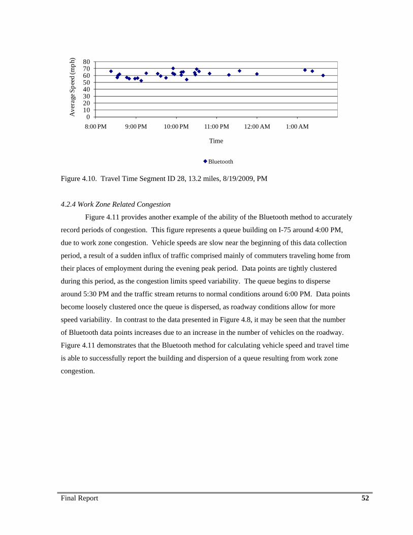
Final Report 52

01020304050607080

8:00 PM 9:00 PM 10:00 PM 11:00 PM 12:00 AM 1:00 AM

Ave

rage

Spe

ed (m

ph).

Time

Bluetooth

Figure 4.10. Travel Time Segment ID 28, 13.2 miles, 8/19/2009, PM

4.2.4 Work Zone Related Congestion

Figure 4.11 provides another example of the ability of the Bluetooth method to accurately

record periods of congestion. This figure represents a queue building on I-75 around 4:00 PM,

due to work zone congestion. Vehicle speeds are slow near the beginning of this data collection

period, a result of a sudden influx of traffic comprised mainly of commuters traveling home from

their places of employment during the evening peak period. Data points are tightly clustered

during this period, as the congestion limits speed variability. The queue begins to disperse

around 5:30 PM and the traffic stream returns to normal conditions around 6:00 PM. Data points

become loosely clustered once the queue is dispersed, as roadway conditions allow for more

speed variability. In contrast to the data presented in Figure 4.8, it may be seen that the number

of Bluetooth data points increases due to an increase in the number of vehicles on the roadway.

Figure 4.11 demonstrates that the Bluetooth method for calculating vehicle speed and travel time

is able to successfully report the building and dispersion of a queue resulting from work zone

congestion.

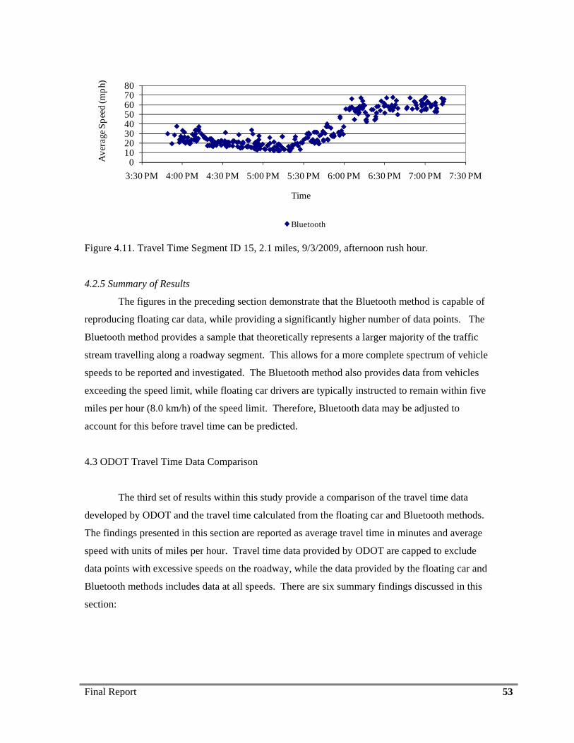
Final Report 53

01020304050607080


Ave

rage

Spe

ed (m

ph).

Time

Bluetooth


4.2.5 Summary of Results

The figures in the preceding section demonstrate that the Bluetooth method is capable of

reproducing floating car data, while providing a significantly higher number of data points. The

Bluetooth method provides a sample that theoretically represents a larger majority of the traffic

stream travelling along a roadway segment. This allows for a more complete spectrum of vehicle

speeds to be reported and investigated. The Bluetooth method also provides data from vehicles

exceeding the speed limit, while floating car drivers are typically instructed to remain within five

miles per hour (8.0 km/h) of the speed limit. Therefore, Bluetooth data may be adjusted to

account for this before travel time can be predicted.

4.3 ODOT Travel Time Data Comparison

The third set of results within this study provide a comparison of the travel time data

developed by ODOT and the travel time calculated from the floating car and Bluetooth methods.

The findings presented in this section are reported as average travel time in minutes and average

speed with units of miles per hour. Travel time data provided by ODOT are capped to exclude

data points with excessive speeds on the roadway, while the data provided by the floating car and

Bluetooth methods includes data at all speeds. There are six summary findings discussed in this

section:

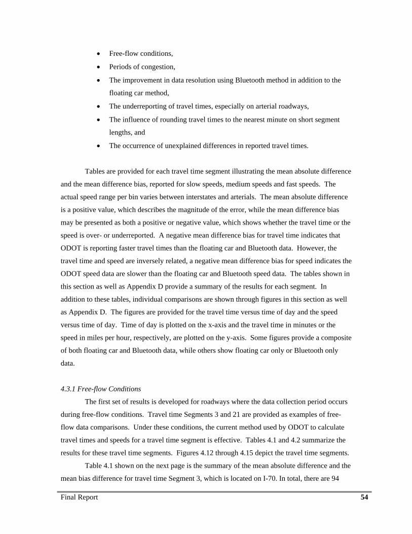
Final Report 54

• Free-flow conditions,

• Periods of congestion,

• The improvement in data resolution using Bluetooth method in addition to the

floating car method,

• The underreporting of travel times, especially on arterial roadways,

• The influence of rounding travel times to the nearest minute on short segment

lengths, and

• The occurrence of unexplained differences in reported travel times.

Tables are provided for each travel time segment illustrating the mean absolute difference

and the mean difference bias, reported for slow speeds, medium speeds and fast speeds. The

actual speed range per bin varies between interstates and arterials. The mean absolute difference

is a positive value, which describes the magnitude of the error, while the mean difference bias

may be presented as both a positive or negative value, which shows whether the travel time or the

speed is over- or underreported. A negative mean difference bias for travel time indicates that

ODOT is reporting faster travel times than the floating car and Bluetooth data. However, the

travel time and speed are inversely related, a negative mean difference bias for speed indicates the

ODOT speed data are slower than the floating car and Bluetooth speed data. The tables shown in

this section as well as Appendix D provide a summary of the results for each segment. In

addition to these tables, individual comparisons are shown through figures in this section as well

as Appendix D. The figures are provided for the travel time versus time of day and the speed

versus time of day. Time of day is plotted on the x-axis and the travel time in minutes or the

speed in miles per hour, respectively, are plotted on the y-axis. Some figures provide a composite

of both floating car and Bluetooth data, while others show floating car only or Bluetooth only

data.

4.3.1 Free-flow Conditions

The first set of results is developed for roadways where the data collection period occurs

during free-flow conditions. Travel time Segments 3 and 21 are provided as examples of free-

flow data comparisons. Under these conditions, the current method used by ODOT to calculate

travel times and speeds for a travel time segment is effective. Tables 4.1 and 4.2 summarize the

results for these travel time segments. Figures 4.12 through 4.15 depict the travel time segments.

Table 4.1 shown on the next page is the summary of the mean absolute difference and the

mean bias difference for travel time Segment 3, which is located on I-70. In total, there are 94

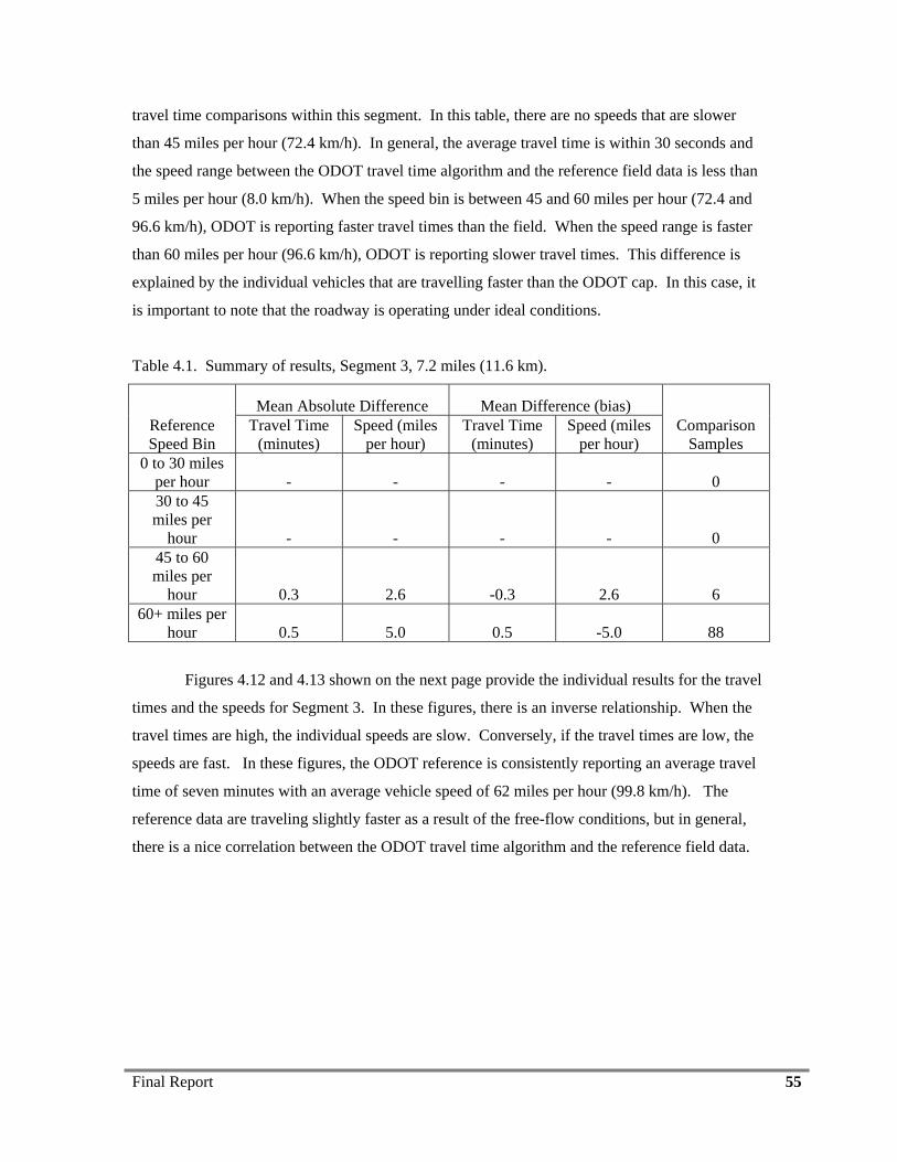
Final Report 55

travel time comparisons within this segment. In this table, there are no speeds that are slower

than 45 miles per hour (72.4 km/h). In general, the average travel time is within 30 seconds and

the speed range between the ODOT travel time algorithm and the reference field data is less than

5 miles per hour (8.0 km/h). When the speed bin is between 45 and 60 miles per hour (72.4 and

96.6 km/h), ODOT is reporting faster travel times than the field. When the speed range is faster

than 60 miles per hour (96.6 km/h), ODOT is reporting slower travel times. This difference is

explained by the individual vehicles that are travelling faster than the ODOT cap. In this case, it

is important to note that the roadway is operating under ideal conditions.

Table 4.1. Summary of results, Segment 3, 7.2 miles (11.6 km).

Reference Speed Bin

Mean Absolute Difference Mean Difference (bias) Comparison

Samples Travel Time

(minutes) Speed (miles

per hour) Travel Time


per hour) 0 to 30 miles

per hour - - - - 0 30 to 45 miles per

hour - - - - 0 45 to 60 miles per

hour 0.3 2.6 -0.3 2.6 6 60+ miles per

hour 0.5 5.0 0.5 -5.0 88

Figures 4.12 and 4.13 shown on the next page provide the individual results for the travel

times and the speeds for Segment 3. In these figures, there is an inverse relationship. When the

travel times are high, the individual speeds are slow. Conversely, if the travel times are low, the

speeds are fast. In these figures, the ODOT reference is consistently reporting an average travel

time of seven minutes with an average vehicle speed of 62 miles per hour (99.8 km/h). The

reference data are traveling slightly faster as a result of the free-flow conditions, but in general,

there is a nice correlation between the ODOT travel time algorithm and the reference field data.

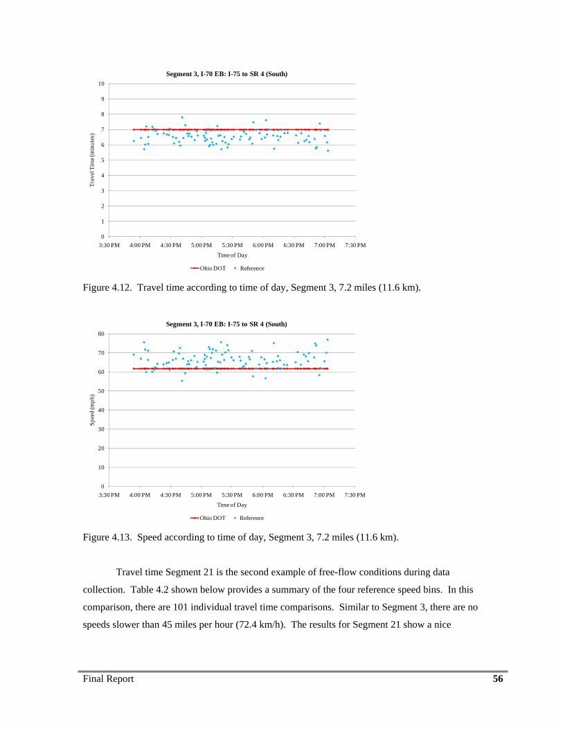
Final Report 56

0

1

2

3

4

5

6

7

8

9

10


Trav

el T

ime (

min

utes

)

Time of Day

Segment 3, I-70 EB: I-75 to SR 4 (South)

Ohio DOT Reference Figure 4.12. Travel time according to time of day, Segment 3, 7.2 miles (11.6 km).

0

10

20

30

40

50

60

70

80


Spee

d (m

ph)

Time of Day


Ohio DOT Reference Figure 4.13. Speed according to time of day, Segment 3, 7.2 miles (11.6 km).

Travel time Segment 21 is the second example of free-flow conditions during data

collection. Table 4.2 shown below provides a summary of the four reference speed bins. In this

comparison, there are 101 individual travel time comparisons. Similar to Segment 3, there are no

speeds slower than 45 miles per hour (72.4 km/h). The results for Segment 21 show a nice

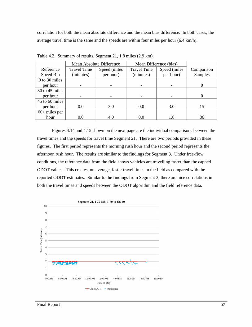
Final Report 57

correlation for both the mean absolute difference and the mean bias difference. In both cases, the

average travel time is the same and the speeds are within four miles per hour (6.4 km/h).


Reference Speed Bin


Samples Travel Time





per hour - - - - 0 30 to 45 miles


per hour 0.0 3.0 0.0 3.0 15 60+ miles per

hour 0.0 4.0 0.0 1.8 86

Figures 4.14 and 4.15 shown on the next page are the individual comparisons between the

travel times and the speeds for travel time Segment 21. There are two periods provided in these

figures. The first period represents the morning rush hour and the second period represents the

afternoon rush hour. The results are similar to the findings for Segment 3. Under free-flow

conditions, the reference data from the field shows vehicles are travelling faster than the capped

ODOT values. This creates, on average, faster travel times in the field as compared with the

reported ODOT estimates. Similar to the findings from Segment 3, there are nice correlations in

both the travel times and speeds between the ODOT algorithm and the field reference data.

0

1

2

3

4

5

6

7

8

9

10

6:00 AM 8:00 AM 10:00 AM 12:00 PM 2:00 PM 4:00 PM 6:00 PM 8:00 PM 10:00 PM

Trav

el T

ime (

min

utes

)

Time of Day

Segment 21, I-75 NB: I-70 to US 40

Ohio DOT Reference

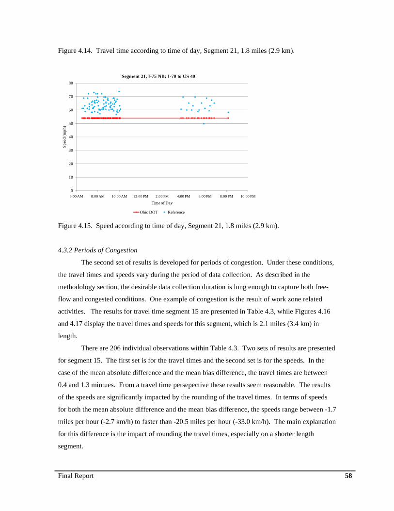
Final Report 58

Figure 4.14. Travel time according to time of day, Segment 21, 1.8 miles (2.9 km).

0

10

20

30

40

50

60

70

80


Spee

d (m

ph)

Time of Day



4.3.2 Periods of Congestion

The second set of results is developed for periods of congestion. Under these conditions,

the travel times and speeds vary during the period of data collection. As described in the

methodology section, the desirable data collection duration is long enough to capture both free-

flow and congested conditions. One example of congestion is the result of work zone related

activities. The results for travel time segment 15 are presented in Table 4.3, while Figures 4.16

and 4.17 display the travel times and speeds for this segment, which is 2.1 miles (3.4 km) in

length.

There are 206 individual observations within Table 4.3. Two sets of results are presented

for segment 15. The first set is for the travel times and the second set is for the speeds. In the

case of the mean absolute difference and the mean bias difference, the travel times are between

0.4 and 1.3 mintues. From a travel time persepective these results seem reasonable. The results

of the speeds are significantly impacted by the rounding of the travel times. In terms of speeds

for both the mean absolute difference and the mean bias difference, the speeds range between -1.7

miles per hour (-2.7 km/h) to faster than -20.5 miles per hour (-33.0 km/h). The main explanation

for this difference is the impact of rounding the travel times, especially on a shorter length

segment.

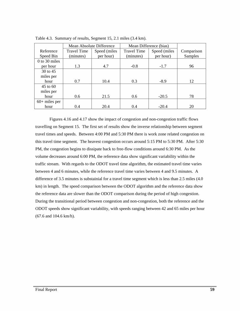
Final Report 59


Reference Speed Bin


Samples Travel Time





per hour 1.3 4.7 -0.8 -1.7 96 30 to 45 miles per

hour 0.7 10.4 0.3 -8.9 12 45 to 60 miles per

hour 0.6 21.5 0.6 -20.5 78 60+ miles per

hour 0.4 20.4 0.4 -20.4 20

Figures 4.16 and 4.17 show the impact of congestion and non-congestion traffic flows

travelling on Segment 15. The first set of results show the inverse relationship between segment

travel times and speeds. Between 4:00 PM and 5:30 PM there is work zone related congestion on

this travel time segment. The heavest congestion occurs around 5:15 PM to 5:30 PM. After 5:30

PM, the congestion begins to dissipate back to free-flow conditions around 6:30 PM. As the

volume decreases around 6:00 PM, the reference data show significant variability within the

traffic stream. With regards to the ODOT travel time algorithm, the estimated travel time varies

between 4 and 6 minutes, while the reference travel time varies between 4 and 9.5 minutes. A

difference of 3.5 minutes is substainial for a travel time segment which is less than 2.5 miles (4.0

km) in length. The speed comparison between the ODOT algorithm and the reference data show

the reference data are slower than the ODOT comparison during the period of high congestion.

During the transitional period between congestion and non-congestion, both the reference and the

ODOT speeds show significant variability, with speeds ranging between 42 and 65 miles per hour

(67.6 and 104.6 km/h).

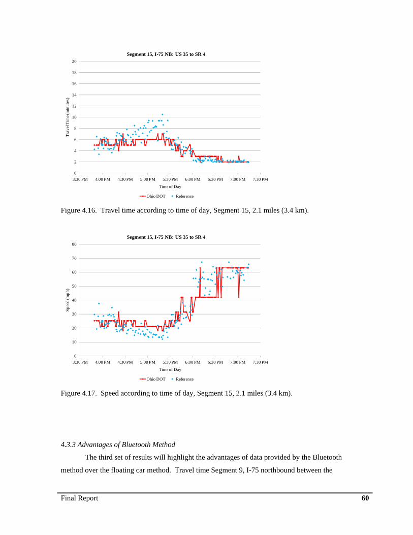
Final Report 60

0

2

4

6

8

10

12

14

16

18

20


Trav

el T

ime (

min

utes

)

Time of Day

Segment 15, I-75 NB: US 35 to SR 4


0

10

20

30

40

50

60

70

80


Spee

d (m

ph)

Time of Day



4.3.3 Advantages of Bluetooth Method

The third set of results will highlight the advantages of data provided by the Bluetooth

method over the floating car method. Travel time Segment 9, I-75 northbound between the

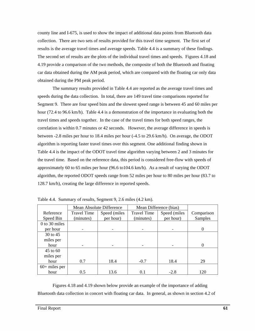
Final Report 61

county line and I-675, is used to show the impact of additional data points from Bluetooth data

collection. There are two sets of results provided for this travel time segment. The first set of

results is the average travel times and average speeds. Table 4.4 is a summary of these findings.

The second set of results are the plots of the individual travel times and speeds. Figures 4.18 and

4.19 provide a comparison of the two methods, the composite of both the Bluetooth and floating

car data obtained during the AM peak period, which are compared with the floating car only data

obtained during the PM peak period.

The summary results provided in Table 4.4 are reported as the average travel times and

speeds during the data collection. In total, there are 149 travel time comparisons reported for

Segment 9. There are four speed bins and the slowest speed range is between 45 and 60 miles per

hour (72.4 to 96.6 km/h). Table 4.4 is a demonstration of the importance in evaluating both the

travel times and speeds together. In the case of the travel times for both speed ranges, the

correlation is within 0.7 minutes or 42 seconds. However, the average difference in speeds is

between -2.8 miles per hour to 18.4 miles per hour (-4.5 to 29.6 km/h). On average, the ODOT

algorithm is reporting faster travel times over this segment. One additional finding shown in

Table 4.4 is the impact of the ODOT travel time algorithm varying between 2 and 3 minutes for

the travel time. Based on the reference data, this period is considered free-flow with speeds of

approximately 60 to 65 miles per hour (96.6 to104.6 km/h). As a result of varying the ODOT

algorithm, the reported ODOT speeds range from 52 miles per hour to 80 miles per hour (83.7 to

128.7 km/h), creating the large difference in reported speeds.


Reference Speed Bin


Samples Travel Time







hour 0.7 18.4 -0.7 18.4 29 60+ miles per

hour 0.5 13.6 0.1 -2.8 120

Figures 4.18 and 4.19 shown below provide an example of the importance of adding

Bluetooth data collection in concert with floating car data. In general, as shown in section 4.2 of

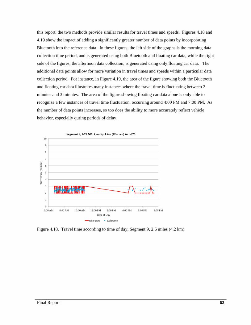
Final Report 62

this report, the two methods provide similar results for travel times and speeds. Figures 4.18 and

4.19 show the impact of adding a significantly greater number of data points by incorporating

Bluetooth into the reference data. In these figures, the left side of the graphs is the morning data

collection time period, and is generated using both Bluetooth and floating car data, while the right

side of the figures, the afternoon data collection, is generated using only floating car data. The

additional data points allow for more variation in travel times and speeds within a particular data

collection period. For instance, in Figure 4.19, the area of the figure showing both the Bluetooth

and floating car data illustrates many instances where the travel time is fluctuating between 2

minutes and 3 minutes. The area of the figure showing floating car data alone is only able to

recognize a few instances of travel time fluctuation, occurring around 4:00 PM and 7:00 PM. As

the number of data points increases, so too does the ability to more accurately reflect vehicle

behavior, especially during periods of delay.

0

1

2

3

4

5

6

7

8

9

10

6:00 AM 8:00 AM 10:00 AM 12:00 PM 2:00 PM 4:00 PM 6:00 PM 8:00 PM

Trav

el T

ime (

min

utes

)

Time of Day

Segment 9, I-75 NB: County Line (Warren) to I-675


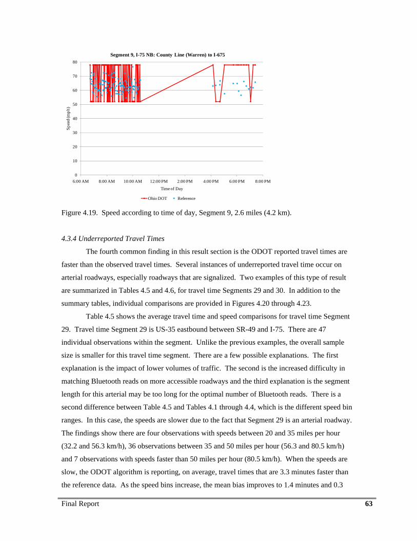
Final Report 63

0

10

20

30

40

50

60

70

80


Spee

d (m

ph)

Time of Day



4.3.4 Underreported Travel Times

The fourth common finding in this result section is the ODOT reported travel times are

faster than the observed travel times. Several instances of underreported travel time occur on

arterial roadways, especially roadways that are signalized. Two examples of this type of result

are summarized in Tables 4.5 and 4.6, for travel time Segments 29 and 30. In addition to the

summary tables, individual comparisons are provided in Figures 4.20 through 4.23.

Table 4.5 shows the average travel time and speed comparisons for travel time Segment

29. Travel time Segment 29 is US-35 eastbound between SR-49 and I-75. There are 47

individual observations within the segment. Unlike the previous examples, the overall sample

size is smaller for this travel time segment. There are a few possible explanations. The first

explanation is the impact of lower volumes of traffic. The second is the increased difficulty in

matching Bluetooth reads on more accessible roadways and the third explanation is the segment

length for this arterial may be too long for the optimal number of Bluetooth reads. There is a

second difference between Table 4.5 and Tables 4.1 through 4.4, which is the different speed bin

ranges. In this case, the speeds are slower due to the fact that Segment 29 is an arterial roadway.

The findings show there are four observations with speeds between 20 and 35 miles per hour

(32.2 and 56.3 km/h), 36 observations between 35 and 50 miles per hour (56.3 and 80.5 km/h)

and 7 observations with speeds faster than 50 miles per hour (80.5 km/h). When the speeds are

slow, the ODOT algorithm is reporting, on average, travel times that are 3.3 minutes faster than

the reference data. As the speed bins increase, the mean bias improves to 1.4 minutes and 0.3

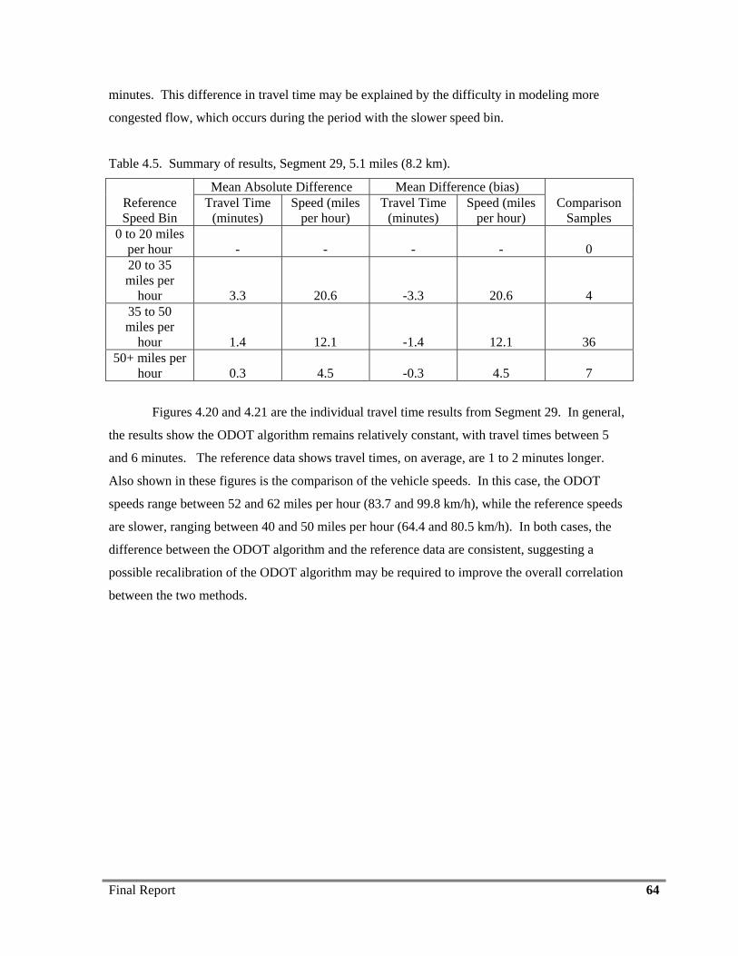
Final Report 64

minutes. This difference in travel time may be explained by the difficulty in modeling more

congested flow, which occurs during the period with the slower speed bin.


Reference Speed Bin


Samples Travel Time






hour 3.3 20.6 -3.3 20.6 4 35 to 50 miles per

hour 1.4 12.1 -1.4 12.1 36 50+ miles per

hour 0.3 4.5 -0.3 4.5 7

Figures 4.20 and 4.21 are the individual travel time results from Segment 29. In general,

the results show the ODOT algorithm remains relatively constant, with travel times between 5

and 6 minutes. The reference data shows travel times, on average, are 1 to 2 minutes longer.

Also shown in these figures is the comparison of the vehicle speeds. In this case, the ODOT

speeds range between 52 and 62 miles per hour (83.7 and 99.8 km/h), while the reference speeds

are slower, ranging between 40 and 50 miles per hour (64.4 and 80.5 km/h). In both cases, the

difference between the ODOT algorithm and the reference data are consistent, suggesting a

possible recalibration of the ODOT algorithm may be required to improve the overall correlation

between the two methods.

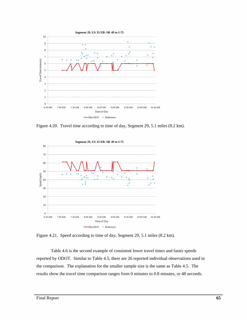
Final Report 65

0

1

2

3

4

5

6

7

8

9

10


Trav

el T

ime (

min

utes

)

Time of Day

Segment 29, US 35 EB: SR 49 to I-75


0

10

20

30

40

50

60

70

80


Spee

d (m

ph)

Time of Day



Table 4.6 is the second example of consistent lower travel times and faster speeds

reported by ODOT. Similar to Table 4.5, there are 26 reported individual observations used in

the comparison. The explanation for the smaller sample size is the same as Table 4.5. The

results show the travel time comparison ranges from 0 minutes to 0.8 minutes, or 48 seconds.

Final Report 66

Based on the mean bias difference, on average, the ODOT algorithm is reporting faster travel

times than the reference data.


Reference Speed Bin


Samples Travel Time







hour 0.8 6.3 -0.8 6.3 21 50+ miles per

hour 0.4 3.6 0.0 0.7 5

Figures 4.22 and 4.23 shown on the next page are developed for Segment 30. In this

comparison, the ODOT travel time algorithm varies between 5 and 7 minutes, while the reference

travel times remain near 6.5 to 7 minutes. The change in travel times corresponds to an estimated

speed of 52 to 62 miles per hour (83.7 and 99.8 km/h) for the ODOT algorithm and 42 to 50 miles

per hour (67.6 and 80.5 km/h) for the reference data. In general, the results remain consistent

with the ODOT algorithm, estimating slightly faster travel times. One potential improvement,

which is similar to Figures 4.20 and 4.21, is the recalibration of the ODOT algorithm, which may

include adding 1 to 2 minutes to the travel time estimate.

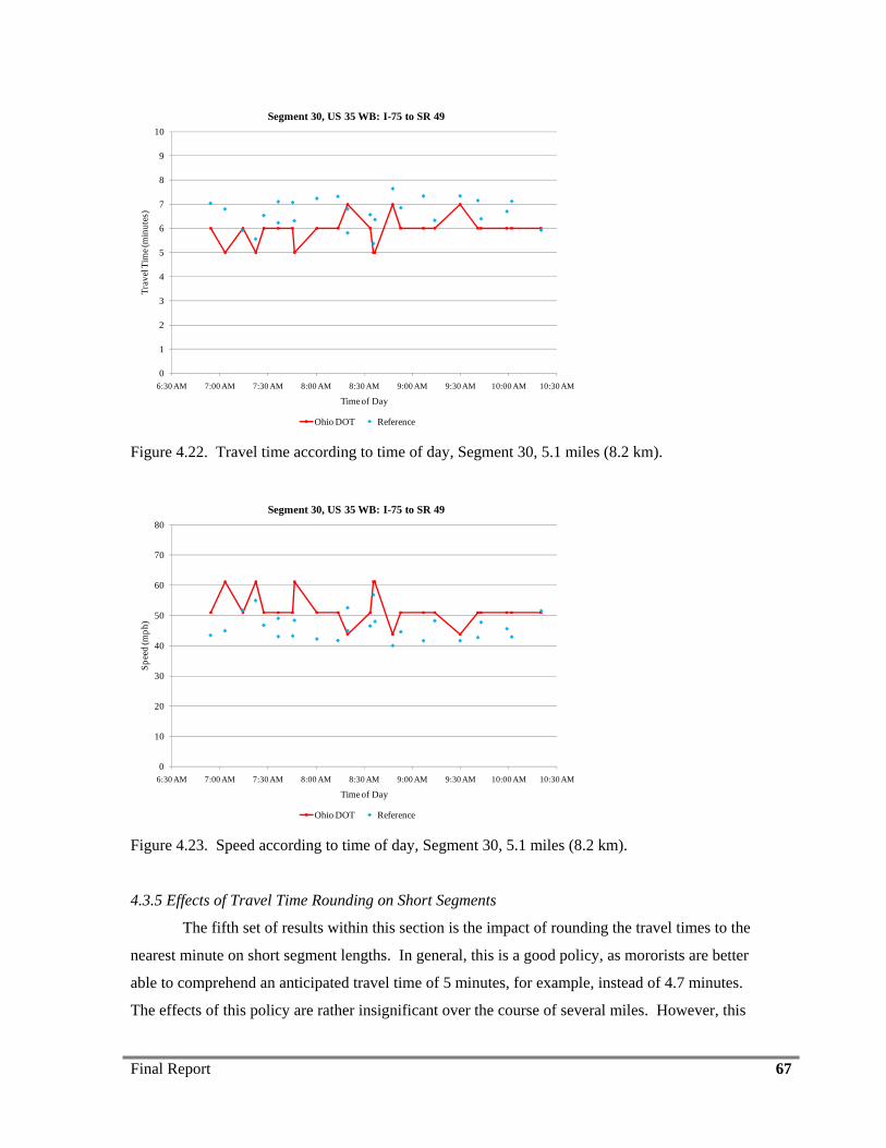
Final Report 67

0

1

2

3

4

5

6

7

8

9

10


Trav

el T

ime (

min

utes

)

Time of Day

Segment 30, US 35 WB: I-75 to SR 49


0

10

20

30

40

50

60

70

80


Spee

d (m

ph)

Time of Day



4.3.5 Effects of Travel Time Rounding on Short Segments

The fifth set of results within this section is the impact of rounding the travel times to the

nearest minute on short segment lengths. In general, this is a good policy, as mororists are better

able to comprehend an anticipated travel time of 5 minutes, for example, instead of 4.7 minutes.

The effects of this policy are rather insignificant over the course of several miles. However, this

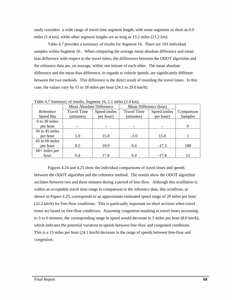
Final Report 68

study considers a wide range of travel time segment length, with some segments as short as 0.9

miles (1.4 km), while other segment lengths are as long as 13.2 miles (21.2 km).

Table 4.7 provides a summary of results for Segment 16. There are 193 individual

samples within Segment 16. When comparing the average mean absolute difference and mean

bias difference with respect to the travel times, the differences between the ODOT algorithm and

the reference data are, on average, within one minute of each other. The mean absolute

difference and the mean bias difference, in regards to vehicle speeds, are significantly different

between the two methods. This difference is the direct result of rounding the travel times. In this

case, the values vary by 15 to 18 miles per hour (24.1 to 29.0 km/h).

Table 4.7 Summary of results, Segment 16, 2.1 miles (3.4 km).

Reference Speed Bin


Samples Travel Time






per hour 1.0 15.0 -1.0 15.0 1 45 to 60 miles

per hour 0.5 18.9 0.4 -17.3 180 60+ miles per

hour 0.4 17.8 0.4 -17.8 12

Figures 4.24 and 4.25 show the individual comparisons of travel times and speeds

between the ODOT algorithm and the reference method. The results show the ODOT algorithm

oscilates between two and three minutes during a period of free-flow. Although this ocsillation is

within an acceptable travel time range in comparison to the reference data, this ocialltion, as

shown in Figure 4.25, corresponds to an approximate estimated speed range of 20 miles per hour

(32.2 km/h) for free-flow conditions. This is particually important on short sections when travel

times are based on free-flow conditions. Assuming congestion resulting in travel times increasing

to 5 to 6 minutes, the corresponding range in speed would decrease to 5 miles per hour (8.0 km/h),

which indicates the potential variation in speeds between free-flow and congested conditions.

This is a 15 miles per hour (24.1 km/h) decrease in the range of speeds between free-flow and

congestion.

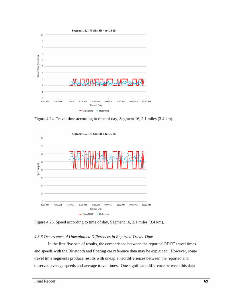
Final Report 69

0

1

2

3

4

5

6

7

8

9

10


Trav

el T

ime (

min

utes

)

Time of Day

Segment 16, I-75 SB: SR 4 to US 35


0

10

20

30

40

50

60

70

80


Spee

d (m

ph)

Time of Day



4.3.6 Occurrence of Unexplained Differences in Reported Travel Time

In the first five sets of results, the comparisons between the reported ODOT travel times

and speeds with the Bluetooth and floating car reference data may be explained. However, some

travel time segments produce results with unexplained differences between the reported and

observed average speeds and average travel times. One significant difference between this data

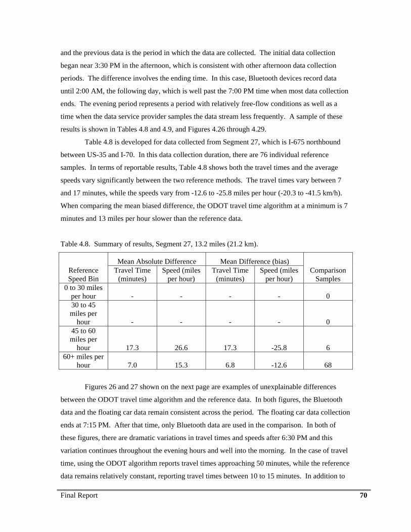
Final Report 70

and the previous data is the period in which the data are collected. The initial data collection

began near 3:30 PM in the afternoon, which is consistent with other afternoon data collection

periods. The difference involves the ending time. In this case, Bluetooth devices record data

until 2:00 AM, the following day, which is well past the 7:00 PM time when most data collection

ends. The evening period represents a period with relatively free-flow conditions as well as a

time when the data service provider samples the data stream less frequently. A sample of these

results is shown in Tables 4.8 and 4.9, and Figures 4.26 through 4.29.

Table 4.8 is developed for data collected from Segment 27, which is I-675 northbound

between US-35 and I-70. In this data collection duration, there are 76 individual reference

samples. In terms of reportable results, Table 4.8 shows both the travel times and the average

speeds vary significantly between the two reference methods. The travel times vary between 7

and 17 minutes, while the speeds vary from -12.6 to -25.8 miles per hour (-20.3 to -41.5 km/h).

When comparing the mean biased difference, the ODOT travel time algorithm at a minimum is 7

minutes and 13 miles per hour slower than the reference data.


Reference Speed Bin


Samples Travel Time







hour 17.3 26.6 17.3 -25.8 6 60+ miles per

hour 7.0 15.3 6.8 -12.6 68

Figures 26 and 27 shown on the next page are examples of unexplainable differences

between the ODOT travel time algorithm and the reference data. In both figures, the Bluetooth

data and the floating car data remain consistent across the period. The floating car data collection

ends at 7:15 PM. After that time, only Bluetooth data are used in the comparison. In both of

these figures, there are dramatic variations in travel times and speeds after 6:30 PM and this

variation continues throughout the evening hours and well into the morning. In the case of travel

time, using the ODOT algorithm reports travel times approaching 50 minutes, while the reference

data remains relatively constant, reporting travel times between 10 to 15 minutes. In addition to

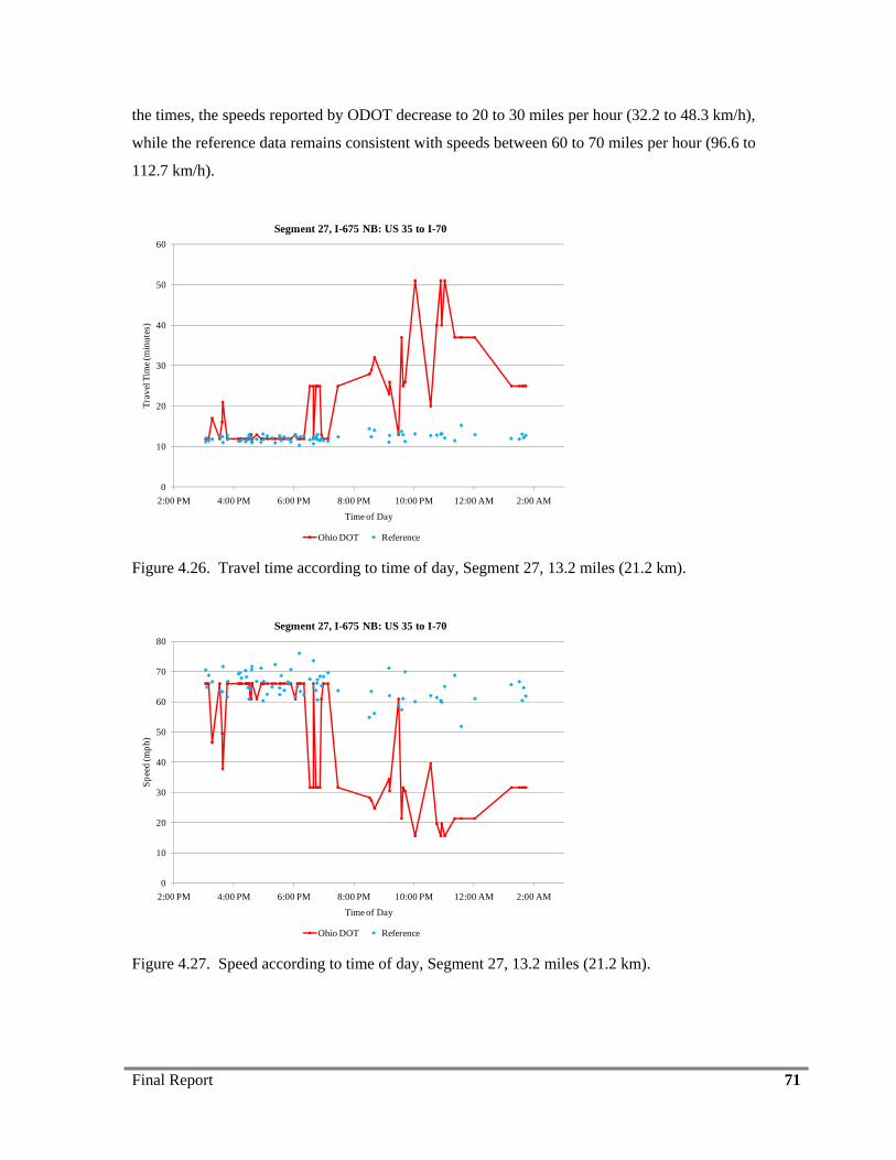
Final Report 71

the times, the speeds reported by ODOT decrease to 20 to 30 miles per hour (32.2 to 48.3 km/h),

while the reference data remains consistent with speeds between 60 to 70 miles per hour (96.6 to

112.7 km/h).

0

10

20

30

40

50

60

2:00 PM 4:00 PM 6:00 PM 8:00 PM 10:00 PM 12:00 AM 2:00 AM

Trav

el T

ime (

min

utes

)

Time of Day

Segment 27, I-675 NB: US 35 to I-70


0

10

20

30

40

50

60

70

80

2:00 PM 4:00 PM 6:00 PM 8:00 PM 10:00 PM 12:00 AM 2:00 AM

Spee

d (m

ph)

Time of Day



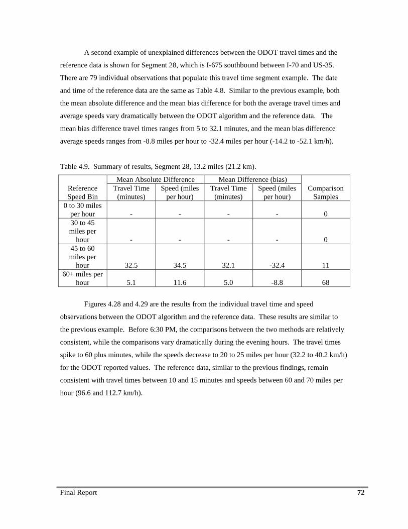
Final Report 72

A second example of unexplained differences between the ODOT travel times and the

reference data is shown for Segment 28, which is I-675 southbound between I-70 and US-35.

There are 79 individual observations that populate this travel time segment example. The date

and time of the reference data are the same as Table 4.8. Similar to the previous example, both

the mean absolute difference and the mean bias difference for both the average travel times and

average speeds vary dramatically between the ODOT algorithm and the reference data. The

mean bias difference travel times ranges from 5 to 32.1 minutes, and the mean bias difference

average speeds ranges from -8.8 miles per hour to -32.4 miles per hour (-14.2 to -52.1 km/h).


Reference Speed Bin


Samples Travel Time







hour 32.5 34.5 32.1 -32.4 11 60+ miles per

hour 5.1 11.6 5.0 -8.8 68

Figures 4.28 and 4.29 are the results from the individual travel time and speed

observations between the ODOT algorithm and the reference data. These results are similar to

the previous example. Before 6:30 PM, the comparisons between the two methods are relatively

consistent, while the comparisons vary dramatically during the evening hours. The travel times

spike to 60 plus minutes, while the speeds decrease to 20 to 25 miles per hour (32.2 to 40.2 km/h)

for the ODOT reported values. The reference data, similar to the previous findings, remain

consistent with travel times between 10 and 15 minutes and speeds between 60 and 70 miles per

hour (96.6 and 112.7 km/h).

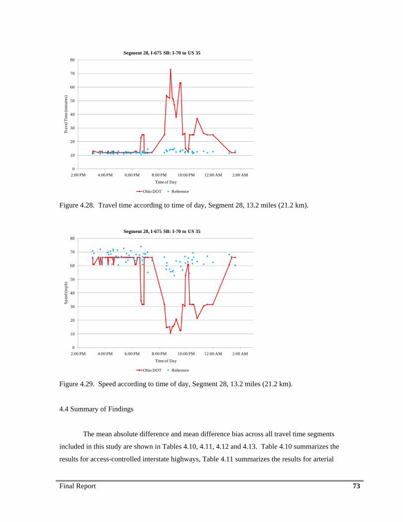
Final Report 73

0

10

20

30

40

50

60

70

80

2:00 PM 4:00 PM 6:00 PM 8:00 PM 10:00 PM 12:00 AM 2:00 AM

Trav

el T

ime (

min

utes

)

Time of Day

Segment 28, I-675 SB: I-70 to US 35


0

10

20

30

40

50

60

70

80

2:00 PM 4:00 PM 6:00 PM 8:00 PM 10:00 PM 12:00 AM 2:00 AM

Spee

d (m

ph)

Time of Day



4.4 Summary of Findings

The mean absolute difference and mean difference bias across all travel time segments

included in this study are shown in Tables 4.10, 4.11, 4.12 and 4.13. Table 4.10 summarizes the

results for access-controlled interstate highways, Table 4.11 summarizes the results for arterial

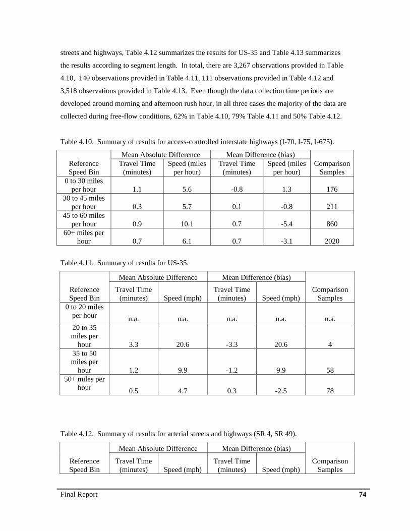
Final Report 74

streets and highways, Table 4.12 summarizes the results for US-35 and Table 4.13 summarizes

the results according to segment length. In total, there are 3,267 observations provided in Table

4.10, 140 observations provided in Table 4.11, 111 observations provided in Table 4.12 and

3,518 observations provided in Table 4.13. Even though the data collection time periods are

developed around morning and afternoon rush hour, in all three cases the majority of the data are

collected during free-flow conditions, 62% in Table 4.10, 79% Table 4.11 and 50% Table 4.12.

Table 4.10. Summary of results for access-controlled interstate highways (I-70, I-75, I-675).

Reference Speed Bin


Samples Travel Time





per hour 1.1 5.6 -0.8 1.3 176 30 to 45 miles

per hour 0.3 5.7 0.1 -0.8 211 45 to 60 miles

per hour 0.9 10.1 0.7 -5.4 860 60+ miles per

hour 0.7 6.1 0.7 -3.1 2020

Table 4.11. Summary of results for US-35.

Reference Speed Bin

Mean Absolute Difference Mean Difference (bias)

Comparison Samples

Travel Time (minutes) Speed (mph)


0 to 20 miles per hour n.a. n.a. n.a. n.a. n.a. 20 to 35 miles per

hour 3.3 20.6 -3.3 20.6 4 35 to 50 miles per

hour 1.2 9.9 -1.2 9.9 58 50+ miles per

hour 0.5 4.7 0.3 -2.5 78

Table 4.12. Summary of results for arterial streets and highways (SR 4, SR 49).

Reference Speed Bin

Mean Absolute Difference Mean Difference (bias)

Comparison Samples



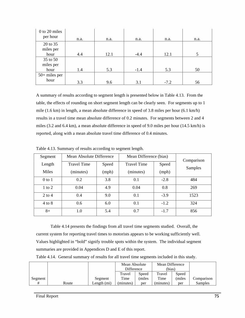
Final Report 75

0 to 20 miles per hour n.a. n.a. n.a. n.a. n.a. 20 to 35 miles per

hour 4.4 12.1 -4.4 12.1 5 35 to 50 miles per

hour 1.4 5.3 -1.4 5.3 50 50+ miles per

hour 3.3 9.6 3.1 -7.2 56

A summary of results according to segment length is presented below in Table 4.13. From the

table, the effects of rounding on short segment length can be clearly seen. For segments up to 1

mile (1.6 km) in length, a mean absolute difference in speed of 3.8 miles per hour (6.1 km/h)

results in a travel time mean absolute difference of 0.2 minutes. For segments between 2 and 4

miles (3.2 and 6.4 km), a mean absolute difference in speed of 9.0 miles per hour (14.5 km/h) is

reported, along with a mean absolute travel time difference of 0.4 minutes.

Table 4.13. Summary of results according to segment length.

Segment

Length

Miles


Samples Travel Time

(minutes)

Speed

(mph)

Travel Time

(minutes)

Speed

(mph)

0 to 1 0.2 3.8 0.1 -2.8 484

1 to 2 0.04 4.9 0.04 0.8 269

2 to 4 0.4 9.0 0.1 -3.9 1523

4 to 8 0.6 6.0 0.1 -1.2 324

8+ 1.0 5.4 0.7 -1.7 856

Table 4.14 presents the findings from all travel time segments studied. Overall, the

current system for reporting travel times to motorists appears to be working sufficiently well.

Values highlighted in “bold” signify trouble spots within the system. The individual segment

summaries are provided in Appendices D and E of this report.

Table 4.14. General summary of results for all travel time segments included in this study.

Segment # Route

Segment Length (mi)

Mean Absolute Difference

Mean Difference (bias)

Comparison Samples

Travel Time

(minutes)

Speed (miles

per

Travel Time

(minutes)

Speed (miles

per

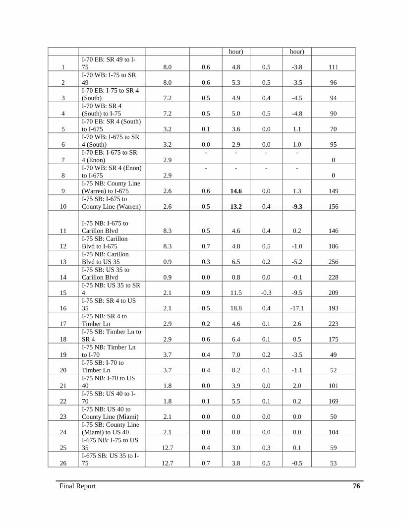
Final Report 76

hour) hour)

1 I-70 EB: SR 49 to I-75 8.0 0.6 4.8 0.5 -3.8 111

2 I-70 WB: I-75 to SR 49 8.0 0.6 5.3 0.5 -3.5 96

3 I-70 EB: I-75 to SR 4 (South) 7.2 0.5 4.9 0.4 -4.5 94

4 I-70 WB: SR 4 (South) to I-75 7.2 0.5 5.0 0.5 -4.8 90

5 I-70 EB: SR 4 (South) to I-675 3.2 0.1 3.6 0.0 1.1 70

6 I-70 WB: I-675 to SR 4 (South) 3.2 0.0 2.9 0.0 1.0 95

7 I-70 EB: I-675 to SR 4 (Enon) 2.9

- - - - 0

8 I-70 WB: SR 4 (Enon) to I-675 2.9

- - - - 0

9 I-75 NB: County Line (Warren) to I-675 2.6 0.6 14.6 0.0 1.3 149

10 I-75 SB: I-675 to County Line (Warren) 2.6 0.5 13.2 0.4 -9.3 156

11 I-75 NB: I-675 to Carillon Blvd 8.3 0.5 4.6 0.4 0.2 146

12 I-75 SB: Carillon Blvd to I-675 8.3 0.7 4.8 0.5 -1.0 186

13 I-75 NB: Carillon Blvd to US 35 0.9 0.3 6.5 0.2 -5.2 256

14 I-75 SB: US 35 to Carillon Blvd 0.9 0.0 0.8 0.0 -0.1 228

15 I-75 NB: US 35 to SR 4 2.1 0.9 11.5 -0.3 -9.5 209

16 I-75 SB: SR 4 to US 35 2.1 0.5 18.8 0.4 -17.1 193

17 I-75 NB: SR 4 to Timber Ln 2.9 0.2 4.6 0.1 2.6 223

18 I-75 SB: Timber Ln to SR 4 2.9 0.6 6.4 0.1 0.5 175

19 I-75 NB: Timber Ln to I-70 3.7 0.4 7.0 0.2 -3.5 49

20 I-75 SB: I-70 to Timber Ln 3.7 0.4 8.2 0.1 -1.1 52

21 I-75 NB: I-70 to US 40 1.8 0.0 3.9 0.0 2.0 101

22 I-75 SB: US 40 to I-70 1.8 0.1 5.5 0.1 0.2 169

23 I-75 NB: US 40 to County Line (Miami) 2.1 0.0 0.0 0.0 0.0 50

24 I-75 SB: County Line (Miami) to US 40 2.1 0.0 0.0 0.0 0.0 104

25 I-675 NB: I-75 to US 35 12.7 0.4 3.0 0.3 0.1 59

26 I-675 SB: US 35 to I-75 12.7 0.7 3.8 0.5 -0.5 53

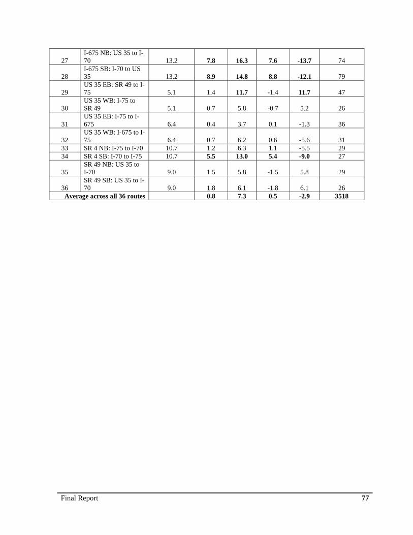
Final Report 77

27 I-675 NB: US 35 to I-70 13.2 7.8 16.3 7.6 -13.7 74

28 I-675 SB: I-70 to US 35 13.2 8.9 14.8 8.8 -12.1 79

29 US 35 EB: SR 49 to I-75 5.1 1.4 11.7 -1.4 11.7 47

30 US 35 WB: I-75 to SR 49 5.1 0.7 5.8 -0.7 5.2 26

31 US 35 EB: I-75 to I-675 6.4 0.4 3.7 0.1 -1.3 36

32 US 35 WB: I-675 to I-75 6.4 0.7 6.2 0.6 -5.6 31

33 SR 4 NB: I-75 to I-70 10.7 1.2 6.3 1.1 -5.5 29 34 SR 4 SB: I-70 to I-75 10.7 5.5 13.0 5.4 -9.0 27

35 SR 49 NB: US 35 to I-70 9.0 1.5 5.8 -1.5 5.8 29

36 SR 49 SB: US 35 to I-70 9.0 1.8 6.1 -1.8 6.1 26

Average across all 36 routes 0.8 7.3 0.5 -2.9 3518

Final Report 78

CHAPTER V

CONCLUSIONS AND RECOMMENDATIONS

5.1 Introduction

Chapter V provides the conclusions and recommendations from this research study. Over

the five data collection trips, data are collected from three main sources used to record vehicle

speeds. The first source is spot speeds, the second source is a traditional approach using floating

car probe data and the third source is a newly developed technique using Bluetooth device

matches. These three methods for estimating traffic flow, more specifically vehicle speed over a

segment of roadway, are used to estimate the actual travel time required by a driver to travel

between the beginning and ending mile point of the 36 travel time segments located in Dayton,

Ohio. These estimated travel times are then posted on changeable message boards for real-time

route information. If the travel times are inaccurate, the posted information will not provide

additional benefit to the user. To ensure accuracy of the estimated travel times, it is paramount

that the system used with these estimations is audited for accuracy. In this study, the conclusions

are presented concerning the following subject matters:

• Comparison between spot speed readings and sensor speeds,

• Evaluation of Bluetooth and floating car methods, and

• The comparisons of ODOT travel times and speeds with field reference data.

Brief descriptions of each task along with recommendations derived from the assessment

of the results are provided in the following sections.

5.2 Comparison Between Spot Speed Readings and Sensor Speeds

The first conclusion is based on the comparison between spot speed readings and sensor

speeds. Shown in Figure 3.1 of the methodology section, there are many radar speed locations

throughout Dayton that are used as part of the ODOT travel time algorithm to estimate speeds. If

the speeds recorded from the spot speed locations are inaccurate, reading faster or slower than the

actual traffic stream, it may lead to inaccurate input into the ODOT travel time algorithm.

Although there are many radar device locations within the study area, the research team sampled

Final Report 79

areas with known congestion as well as individual devices within the travel time segment area. In

most cases, spot speed comparisons are made during data collection runs. In the data collection

associated with the spot speeds, the research team uses laser guns, which sample across all lanes

of traffic in random order for a period of 25 minutes. The collected speeds are then averaged on a

per minute basis and compared with the ODOT reported speeds based on the device id. Figure

4.4 in the results section shows on average, 75% of the one-minute intervals are within the ODOT

required four miles per hour range (6.4 km/h).

There are only a few samples that are significantly different between the field data and

the radar device data. In some cases, these differences may be the result of highly variable traffic

in combination with the location for which each device recorded speeds. In some cases, due to

safety reasons and limited accessibility, the research team is not able to sample in the most

desirable location. A second reason for the difference is the influence of the sample size. The

field data collection team is not able to capture the speeds of each individual vehicle within the

traffic stream, and therefore a random sampling technique is used. Unfortunately, this technique

does not record speeds for all vehicles, especially during high volume free-flow conditions. The

difference in sample size may lead to minor differences between the two speeds recorded at one

location. One additional finding is the impact of weather. On several instances, no field data are

able to be collected during periods with rain. In general, the overall findings suggest that the spot

speeds sampled during this study are valid data inputs for the travel time algorithm.

5.3 Evaluation of Bluetooth and Floating Car Methods

The second source for recording vehicle speed is the use of floating car probe data, with a

relatively new technique using Bluetooth device matches. For the majority of the data collection,

floating car and Bluetooth data are collected at the same time. In this study, three floating car

vehicles are used for data collection, with the exception of SR-49. In the case of SR-49, due to

the travel time segment length and the anticipated low traffic volumes, an additional fourth

vehicle is used in the floating car data collection. After the data collection, the results from each

method are compared against each other. The ultimate goal is highly correlated average speeds

between both methods. In this study, field data are collected on three high volume access-

controlled interstate highways, I-70, I-75 and I-675, an urban arterial highway, US-35, and two

state highways SR-4 and SR-49.

Final Report 80


The first series of roads are high volume access-controlled interstate highways. For these

roads there are several key variables required for an implementable data collection plan. In this

study, the majority of the data are collected during the morning and afternoon rush hour periods.

These periods are selected based on the increased traffic volume, which may lead to more

dynamic changes to the highway in question. In general, there are several findings within this

class of highway. The first finding is developed for periods when vehicles are operating under

free-flow conditions. When the vehicles are travelling under free-flow conditions, the Bluetooth

devices may have a tendency to record slightly faster speeds in comparison to the floating car

data. The main explanation for this is the drivers of the floating cars are instructed to maintain

“normal” speeds close to the posted speed limit, while there are no limitations placed on the

Bluetooth data. These results are easily remedied by placing a capped or maximum speed on the

Bluetooth data. In both cases, the two methods are highly correlated and show free-flow activity

on the travel time segments.

A second set of results shows there are significantly higher numbers of data points for the

Bluetooth devices in comparison to the floating car data. The increased number of points may

not be of great significance under free-flow conditions, but is extremely effective in describing

periods of high variability, for example Figure 4.6. The higher number of points also provides a

greater confidence in estimating the actual speed along a segment of highway. The third finding

of significance is the impact of the segment length. In the case of the floating car data, the travel

time length is not a limiting factor. The drivers are instructed to begin and end their individual

runs at fixed points. The Bluetooth devices are not independent of segment length. As the

segment length increases the number of potential Bluetooth matches decreases. An example of

the decrease in matches is shown in comparing an average data collection period on I-75,

relatively short segment lengths, with I-675, relatively long 12 to 13 mile (19.3 to 20.9 km)

segment lengths. The number of observations is more than half the I-75 data. In comparison to

floating car data, the Bluetooth method for high volume access-controlled highways provides

significantly more data points and increases the overall resolution of the traffic stream.

5.3.2 Arterial Highways

The second class of roadways sampled in this study is arterial highways. In these

samples, the results between the two methods vary. In most cases, the reported speeds remain

consistent and well correlated. There are, however, several limitations associated with the use of

Final Report 81

Bluetooth data. Unlike the previous class of highways, the total volume of vehicles with

Bluetooth devices decreases significantly for vehicles that travel on arterial highways between the

beginning and ending travel time segment mile points. As a result of the lower volumes of traffic,

the number of Bluetooth matches is highly influenced by the length and the accessibility of the

arterial highway. For example there are two, one northbound and one southbound, nine mile

(14.5 km) travel time segments on SR-49. This segment length, in association with areas with

commercial activity, surpasses the capabilities of the Bluetooth data collection. In this example,

there are more data points from the four floating cars than Bluetooth matches. In order to

improve the efficiency and capabilities of the Bluetooth devices, it is recommended that either the

number of travel time segments is increased, lowering the length between end points, or

additional Bluetooth readers should be included throughout the studied segments.

5.4 The Statistical Evaluation of ODOT Travel Times and Speeds with Field Reference Data

The third set of conclusions are based on the statistical evaluation of the reported ODOT

travel time algorithms and the field reference data provided by the floating car and the Bluetooth

method. In this evaluation, findings are calculated for both the average travel times and speeds

during the entire data collection as well as the individual sample comparisons. There are six

conclusions discussed in this section: free-flow conditions, congestion, data resolution using

Bluetooth methods, the underreporting of travel times especially on arterial highways, the

influence of rounding travel times to the nearest minute on short segment lengths and unexplained

differences in reported travel times.

5.4.1 Free-flow Conditions

The first evaluation of the ODOT travel time algorithm is developed under free-flow

conditions. During this study, between 53% and 62% of the samples are collected during free-

flow conditions. In these cases, the overall findings between the reference data and the ODOT

travel time algorithm show slightly faster travel times and speeds for the reference data when

compared with the ODOT travel times. The differences are explained by the capped speeds and

the rounding of the travel times. Even though there are some differences between the methods,

the overall results and conclusions show a nice correlation between the two methods. One

potential recommendation is to define the capped speeds based on segment links in-lieu of spot

locations.

Final Report 82

5.4.2 Periods of Congestion

The second evaluation of the ODOT travel time algorithm is developed under periods of

congestion. In this study, the majority of the congestion is associated with morning and afternoon

rush hour and is the direct result of construction related work zones along I-75 near mile marker

54.4. In this case, there are several conclusions that are made. In general, the overall trend in

terms of longer travel times and slower speeds is consistent between the ODOT travel time

algorithm and the reference data, as shown by Figures 4.16 and 4.17. The ODOT travel time

algorithm under congestion in most cases overestimates the actual speeds, which in turn lowers

the corresponding travel time per segment. In most cases, the difference between the ODOT

travel time algorithm and the reference data is between one to three minutes per segment. This

estimate is reasonable under the high variability associated with congestion.

5.4.3 Data Resolution using Bluetooth Method in Addition to the Floating Car Method

The third evaluation of the ODOT travel time algorithm is the impact of data resolution

between the Bluetooth and the floating car methods. In this set of results, especially for the high

volume limited access-controlled interstate highways, there are substantially more Bluetooth

values than floating car data. The improved resolution is particularly significant during periods

of variability and the use of Bluetooth data is highly recommended.

5.4.4 The Underreporting of Travel Times, Especially on Arterial Highways

The fourth evaluation of the ODOT travel time algorithm is the underreporting of travel

times on arterial highways. In this set of results, the overall trends are the same between the

reference data and the ODOT travel time algorithm. The main difference is the consistent under

estimation of travel times using the ODOT travel time algorithm. One potential recommendation

for these results is the re-calibration of the ODOT travel time algorithm. In most cases, the

difference between the two methods is between one and two minutes, and the re-calibration

should be developed specifically for the arterial highways.

5.4.5 Rounding Travel Times to the Nearest Minute on Short Segment Lengths

The fifth evaluation of the ODOT travel time algorithm is the impact of rounding the

travel times to the nearest minute. The rounding of the travel times is one of the variables used to

calculate the average speed across a travel time segment over time. Although from a motorist

point of view there probably is no noticeable difference, there is a significant impact on the

Final Report 83

estimation of speeds. In addition to the rounding of the travel times, there are significant

differences with estimated speeds under both free-flow and congestion conditions. For example,

Segment 16, Figures 4.24 and 4.25, the average travel times range between two and three minutes

under free-flow conditions. The rounding of the travel times under these conditions creates a

speed range between 42 and 62 miles per hour (67.6 and 99.8 km/h), a 20 mile per hour (32.2

km/h) difference. Under a second hypothetical set of conditions, there is congestion on this same

segment and the travel time is now oscillating between five and six minutes. Although the net

difference remains one minute in travel time, the average change in speed between the two travel

times is less than 5 miles per hour (8.0 km/h). In conclusion, the rounding of the travel times,

especially on shorter travel time segments under free flow conditions, produces a significant

change in the average vehicle speeds over the duration of the segment.

One potential recommendation is the development of a calculation procedure for the

minimum route travel times to avoid high equivalent speeds. Several route segments report travel

times with equivalent speeds faster than the posted speed limit and in some cases, the equivalent

speeds are nearly 80 miles per hour (128.7 km/h). The research team believes these high

equivalent speeds may occur because the minimum travel times are calculated at the link level

then rounded at the route segment level. In some cases, rounding differences appear to be causing

this high equivalent speed. Similarly, the travel time rounding associated with short route

segments exaggerates speed changes.

5.4.6 Unexplained Differences in Reported Travel Times

The sixth evalutaion of the ODOT travel time algorithm and the reference data is based

on unexplained differences in reported travel times. In these cases, there are no clear reasons why

the travel times and speeds are significantly different. The first general recommendation is

further analysis of the fixed-point sensor data and the posted travel times. Additional insight may

provide reasons why there are large travel time errors on several routes. For example, there are

large unexplained errors on Segments 27 and 28 during nighttime data collection. A second

recommendation is the review of archived travel times to reveal how often these extreme

fluctuations occur in low-volume traffic conditions. Another recommendation is based on a

cursory analysis of rainfall data and fixed-point sensor data. Preliminary results do not reveal an

obvious connection between heavy rainfall and significant speed errors, however, more samples

should be collected to evaluate the performance of Doppler radar sensor performance under

adverse weather.

Final Report 84

5.5 Conclusion Summary

In conclusion, the use of Bluetooth data along with floating car data provides an effective

methodology used in referencing travel times and speeds over a travel time segment. In terms of

evaluation, the research team recommends the comparison of both travel times and speeds using

the mean absolute difference and the mean bias difference as well as visual observations between

the ODOT travel time estimates and the reference data. In general, the overall results at the

system-wide level seem reasonable. The results for specific travel time segments are found in

Table 4.12 and Appendices D and E of this research report.

Final Report 85

CHAPTER VI

IMPLEMENTATION PLAN

The implementation plan developed from this research study is divided into eight sections.

These sections are described in more detail in the remaining portion of this chapter. Because the

products from this research proposal are clearly defined, the implementation plan is relatively

straightforward. The first product from this research proposal will be an evaluation report that

details whether the travel time data service provider has met the contract requirements in terms of

data quality. There is a possibility that the evaluation procedures developed as part of this ODOT

study could contribute to the development of a national or international standard (such as ASTM

International) for the evaluation of travel time data services. This research team is currently

discussing the development of a standard travel time data evaluation protocol with several other

industry leaders, including both public agencies and private companies. Depending upon the

outcome of these discussions over the next six months, the ODOT research project with approval

from ODOT may serve as:

• A model for the standard evaluation protocol and/or

• To “pilot test” a draft version of the standard evaluation protocol.

6.1 Recommendations for Implementation

The results from this report are based on the statistical validation of travel times provided

by a data service provider. The final results are shown in Table 4.12 and Appendices D and E. In

general, there are two areas for the implementation of these results. The first recommendation is

to develop additional specific language required by the data service vendor in terms of the data

quality. The second implementation is the development of a field reference handbook based on

floating car and Bluetooth data used in evaluation of travel times. The anticipated handbook will

be similar in structure to the FHWA Travel Time Handbook.

6.2 Steps Needed to Implement Findings

The main step required to implement these findings is a continuation of discussions

between the research team and the technical liaisons. These meetings will include discussions on

Final Report 86

data quality requirements as well as the potential development of a “how to” handbook used for

evaluation purposes in other areas of the state.

6.3 Suggested Time Frame for Implementation

This time frame for the implementation of these results is relatively quick for the draft

language. The time frame is based on the time required to adapt the findings and suggestions

from this report in contractual language that will be provided in the future to data service vendors.

The time frame for a draft handbook is six months. Over this time, the research team will work

with the technical liaisons in crafting the appropriate guidance required for field evaluation.

6.4 Expected Benefits from Implementation

The immediate benefit of this research project is an assurance that the travel time data

service does, or does not, meet contract requirements. If the travel time data service does not meet

contract requirements, then Ohio Department of Transportation (ODOT) may not be legally

obligated to pay the data service provider. If the travel time data service does meet contract

requirements, then ODOT will be assured that state funds have been well spent in acquiring this

data service. An additional short-term benefit for ODOT will be the external review of the data.

This external review ensures the accuracy of the data, strengthening the initiative’s credibility

with the public as well as the media. This research will allow ODOT the capability to say an

external agency has reviewed and implemented quality control/quality assurance procedures on

all data provided from the external vendor.

The main long-term benefit is that ODOT may save money and provide this service much

sooner than otherwise possible by purchasing this real-time traffic information service from a

private company instead of installing and maintaining a state-owned traffic sensor network. The

overall findings from the research will provide a long-term cost savings for ODOT whether the

vendor’s travel time data is accurate or inaccurate. If the data is proven to be accurate, ODOT

will be able to use this information to provide reliable travel time information both internally and

externally and will lead to a cost savings. If the research proves the data provided by the vendor

is inaccurate, ODOT will no longer use this vendor or pay for services that are invalid.

Final Report 87

6.5 Potential Risks and Obstacles to Implementation

The current contract provision mentions the accuracy of reported link/route speeds.

However, ODOT is using a modified travel time estimation algorithm based on the spot speeds

provided by the vendor’s sensors. Therefore, if the link/route travel times are inaccurate, the

vendor may claim that the error is caused by ODOT’s algorithm. If ODOT continues to use its

own travel time estimation algorithm, then the contract provisions should be clarified to apply to

the measurement of spot speeds. Additionally, the contract provisions should specify more

details about the measurement of spot speed accuracy, for example how often, how many

locations, how long for each test period.

6.6 Strategies to Overcome Potential Risks and Obstacles

The most effective strategy to overcome this risk is the development of a standard

method used in referencing the accuracy of the data based on reference field data.

6.7 Potential Users and Other Organizations that May be Affected

The potential users of this information will include the ODOT Office of Traffic

Engineering, data service vendors and motorists who are using the travel time information

provided by the changeable message signs in the Dayton, Ohio area.

6.8 Estimated Costs of Implementation

The final cost for implementation is based on the requirements in developing a new

handbook as well as additional training in the operation of the Bluetooth technologies.

Final Report 88

CHAPTER VII

REFERENCES

Bertini, R.L. and S. Tantiyanugulchai. Transit Buses as Traffic Probes: Use of Geolocation Data

for Empirical Evaluation. In Transportation Research Record 1870, TRB, National Research

Council, Washington, D.C., 2004, pp. 35-45.

"Bluetooth Traffic Monitoring Technology - Privacy and Legality Concerns." Traffax, Inc.. 17 May 2008. Traffax, Inc., Web. 10 Sept 2009. <http://www.traffaxinc.com/content/privacy-concerns>.

Breitenberger, S., B. Gruber, M. Neuherz, and R. Kates. Extended Floating Car Data: Traffic

Information Potential and Necessary Penetration Rates. Traffic Engineering and Control,

December 2004, pp. 390-396.

Cetin, M., G.F. List, and Y. Zhou. Factors Affecting Minimum Number of Probes Required for

Reliable Estimation of Travel Time. In Transportation Research Record 1917, TRB, National

Research Council, Washington, D.C., 2005, pp. 37-44.

Chan, K.S., M.L. Tam., and W.H.K. Lama. Using Automatic Vehicle Identification Data for

Estimating Current Travel Times in Hong Kong. Paper submitted for presentation at the

Transportation Research Board Annual Meeting, January 2007.

Chen, M. and S.I.J. Chien. Determining the Number of Probe Vehicles for Freeway Travel Time

Estimation by Microscopic Simulation. In Transportation Research Record 1719, TRB, National

Research Council, Washington, D.C., 2000, pp. 61-68.

Chen, M. and S.I.J. Chien. Dynamic Freeway Travel Time Prediction with Probe Vehicle Data. In

Transportation Research Record 1768, TRB, National Research Council, Washington, D.C.,

2001, pp. 157-161.

Cheu, R.L., C. Xie, and D.H. Lee. Probe Vehicle Population and Sample Size for Arterial Speed

Estimation. In Computer-Aided Civil and Infrastructure Engineering. Vol. 17, 2002, pp. 53-60.

Final Report 89

“Closing the Data Gap: Guidelines for Quality Advanced Traveler Information System (ATIS)

Data.” ITS America and U.S. Department of Transportation. Version 1.0, September 2000.

"Distance Calculation: How to Calculate the Distance Between Two Points on the Earth."

Meridian World Data. Meridian World Data, Inc., Web. 10 Sept 2009.

<http://www.meridianworlddata.com/Distance-Calculation.asp>.

Eisele, W.L. and L.R. Rilett. Statistical Comparison of Travel Time Estimates Obtained from

Intelligent Transportation Systems and Instrumented Test Vehicles. Transportation Research

Record 1804, TRB, National Research Council, Washington, D.C., 2002.

Eisele, W.L. Estimating Travel Time and Variance Using Intelligent Transportation Systems

Data for Real-time and Off-line Transportation Applications. Ph.D. Dissertation, Texas A&M

University. College Station, Texas. May 2001.

Eisele, W.L., L.R. Rilett, K.B. Mhoon, and C.H. Spiegelman. Using Intelligent Transportation

Systems (ITS) Travel Time Data for Multi-Modal Analysis and System Monitoring.


2001.

Ferman, M.A. and D.E. Blumenfeld. Penetration Requirements for Real-Time Traffic Information

from Probe Vehicles. R&D Paper 10,302, General Motors Research & Development Center,

January 10, 2006.

Ferman, M.A., D.E. Blumenfeld, and X. Dai. An Analytical Evaluation of a Real-Time Traffic

Information System Using Probe Vehicles. In Journal of Intelligent Transportation Systems.

Volume 9, No. 1, 2005, pp. 23-34.

Ferman, M.A., D.E. Blumenfeld, X. Dai, and R.P. Roesser. On-the-Road Test of a Probe-Based

Traffic Information System. General Motors Research and Development Center, 2004.

Final Evaluation Report for the CAPITAL-ITS Operational Test and Demonstration Program.

Transportation Studies Center, University of Maryland, May 1997.

Final Report 90

Fontaine, M.D., Yakkala, A.P., and Smith, B.L. Probe Sampling Strategies for Traffic

Monitoring Systems Based on Wireless Location Technology. Report No. FHWA/VTRC 07-

CR12. Virginia Transportation Research Council, January 2007.

Fontaine, M.D. and B.L. Smith. Probe-Based Traffic Monitoring Systems with Wireless

Location Technology: An Investigation of the Relationship Between System Design and

Effectiveness. In Transportation Research Record 1925, TRB, National Research Council,

Washington, D.C., 2005, pp. 3-11.

Fontaine, M.D. and B.L. Smith. Improving the Effectiveness of Traffic Monitoring Based on

Wireless Location Technology. Report No. VTRC 05-R17. Virginia Transportation Research

Council, December 2004.

Frost & Sullivan. Real-Time Traffic Flow Ground Truth Testing Methodology Validation and

Accuracy Measurement. Prepared for Inrix, Inc., September 25, 2006.

Green, M.W., M.D. Fontaine, and B.L. Smith. Investigation of Dynamic Probe Sample

Requirements for Traffic Condition Monitoring. In Transportation Research Record 1870, TRB,

National Research Council, Washington, D.C., 2004, pp. 55-61.

Hellinga, B. and L. Fu. Assessing Expected Accuracy of Probe Vehicle Travel Time Reports. In

Journal of Transportation Engineering, November/December 1999, pp. 524-530.

Hellinga, B.R. and L. Fu Reducing Bias in Probe-Based Arterial Link Travel Time Estimates. In

Transportation Research Part C, Volume 10, 2002, pp. 257-273.

Hoogenboom, M. The Grand Draw. In Traffic Technology International, Oct/Nov 1999, pp. 66-

68.

Innovations in Transportation: GSR Opportunities at CCIT. PowerPoint presentation by the

California Center for Innovative Transportation, October 2004.

Final Report 91

Kothuri, S.M., K. Tufte, S. Ahn, and R.L. Bertini. Using Archived ITS Data to Generate

Improved Freeway Travel Time Estimates. Paper submitted for presentation at the Transportation

Research Board Annual Meeting, January 2007.

Kuchipudi, C.M. and S.I.J. Chien. Development of a Hybrid Model for Dynamic Travel-Time

Prediction. In Transportation Research Record 1855, TRB, National Research Council,

Washington, D.C., 2003, pp. 22-31.

Kwon, J. and K. Petty. Travel Time Prediction Algorithm Scalable to Freeway Networks with

Many Nodes with Arbitrary Travel Routes. In Transportation Research Record 1935, TRB,

National Research Council, Washington, D.C., 2005, pp. 147-153.

Li, R., G. Rose, and M. Sarvi. Evaluation of Speed-Based Travel Time Estimation. Journal of

Transportation Engineering, Vol. 132, Issue 7, July 2006, pp. 540-547.

Monsere, C.M., A. Breakstone, R.L. Bertini, D. Deeter, and G. McGill. Validating Dynamic

Message Sign Freeway Travel Time Messages with Ground Truth Geospatial Data. In


2006, pp. 19-27.

Nanthawichit, C. T. Nakatsuji, and H. Suzuki. Application of Probe-Vehicle Data for Real-Time

Traffic-State Estimation and Short-Term Travel-Time Prediction on a Freeway. In Transportation

Research Record 1855, TRB, National Research Council, Washington, D.C., 2003, pp. 49-59.

Nihan, N.L., M. Leth, and A. Wang. Video Image Processing for Freeway Monitoring and

Control: Evaluation of the Mobilizer. Report No. WA-RD 398.1, Washington State

Transportation Center, Seattle, Washington, November 1995.

Park, D., L.R. Rilett, P. Pattanamekar, and K. Choi. Estimating Travel Time Summary Statistics

of Larger Intervals from Smaller Intervals Without Storing Individual Data. In Transportation


Final Report 92

Quiroga, C. Assessment of Dynamic Message Sign Travel Time Information Accuracy. Paper

presented at the North American Traffic Monitoring Exhibition and Conference (NATMEC),

Madison, Wisconsin, August 2000.

Sanwal, K.K. and J. Walrand. Vehicles as Probes. Report UCB-ITS-PWP-95-11, California

PATH, Richmond, California, 1995.

Smith, B.L. and M.D. Fontaine, Private Sector Provision of Congestion Data, NCHRP Project

70-01 Final Report, February 27, 2007.

Smith, B.L. and M.D. Fontaine. Time Well Spent. Transportation Management and Engineering.

April 2005, pp. 20-22.

Smith, B.L., H. Zhang, M. Fontaine, M. Green. Cell Phone Probes as an ATMS Tool. Smart

Travel Lab Report No. STL-2003-01, University of Virginia, June 2003.

Smith, B.L., R.B. Holt, and B. Park. Travel Time Estimation for Urban Freeway Performance

Measurement: Understanding and Improving Upon the Extrapolation Method. Paper presented at

the 2004 Annual Meeting of the Transportation Research Board, Washington, D.C., January 2004.

Tarnoff, P. J., J.S. Wasson, S.E. Young, N. Ganig, D.M. Bullock, J.R. Sturdevant. The

Continuing Evolution of Travel Time Data Information Collection and Processing. Paper

submitted for presentation at the Transportation Research Board Annual Meeting, January 2009.

Travel Time Estimates, Displays, and Forecasts – Final Report. Technical Report #2, Prepared

for Maricopa County DOT and Arizona DOT by OZ Engineering and Motion Maps, December

2004.

Texas Transportation Institute. Assessment of Dynamic Message Sign Travel Time Information

Accuracy. Texas Department of Transportation—San Antonio District, August 2000.

Toppen, A. and K. Wunderlich. Travel Time Data Collection for Measurement of Advanced

Traveler Information Systems Accuracy. Prepared by Mitretek Systems for Federal Highway

Administration, June 2003.

Final Report 93

Turner, S.M. Advanced Techniques for Travel Time Data Collection. In Transportation


Turner, S.M. and D. J. Holdener. Probe Vehicle Sample Sizes for Real Time Information:

The Houston Experience. In Proceedings of the Sixth International Conference on

Vehicle Navigation and Information Systems, Seattle, Washington, 1995, pp. 3-9.

Turner, S.M., W.L. Eisele, R.J. Benz, D.J. Holdener. Travel Time Data Collection Handbook.

Report No. FHWA-PL-98-035. Federal Highway Administration, March 1998.

Wunnava, S., K. Yen, T. Babij, R. Zavaleta, R. Romero, and C. Archilla. Travel Time Estimation

Using Cell Phones (TTECP) for Highways and Roadways. Prepared by Florida International

University for Florida Department of Transportation, January 29, 2007.

Yganace, J.L., C. Drane, Y.B. Yim, and R. de Lacvivier. Travel Time Estimation of the San

Francisco Bay Area Network using Cellular Phones as Probes. Report UCB-ITS-PWP-2000-18,

California PATH, Richmond, California, 2000.

Final Report 94

APPENDIX A

SPOT SPEEDS

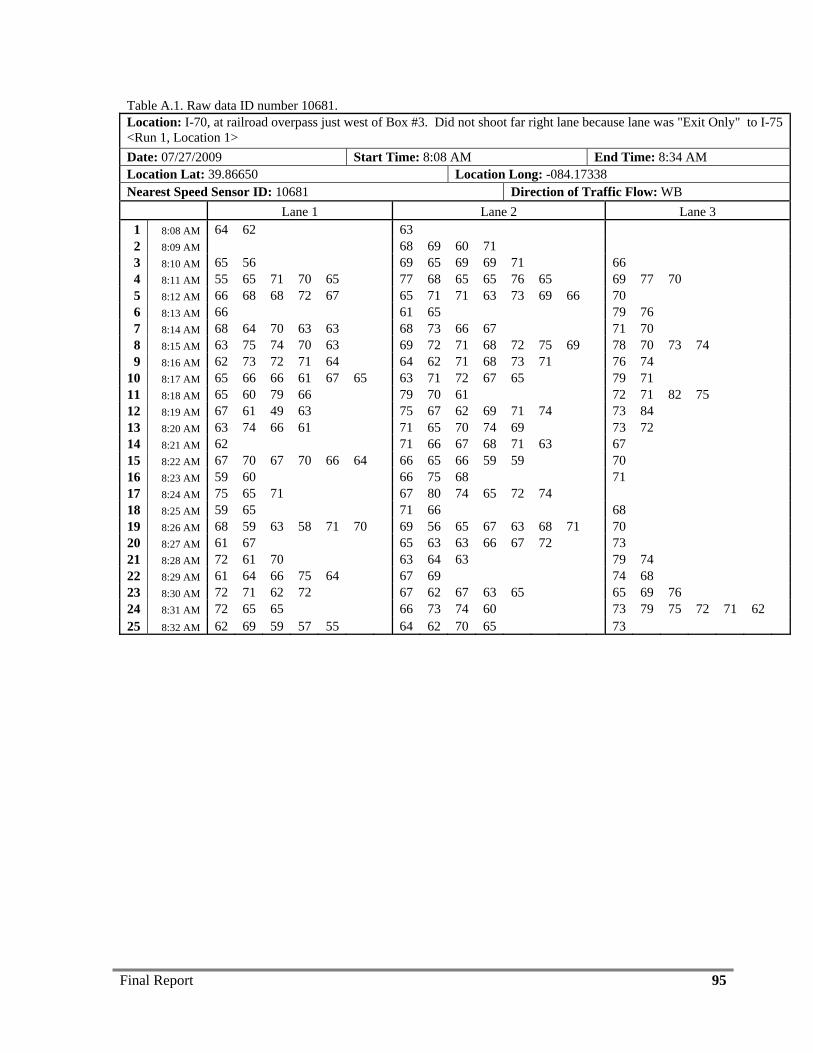
Final Report 95

Table A.1. Raw data ID number 10681. Location: I-70, at railroad overpass just west of Box #3. Did not shoot far right lane because lane was "Exit Only" to I-75 <Run 1, Location 1> Date: 07/27/2009 Start Time: 8:08 AM End Time: 8:34 AM Location Lat: 39.86650 Location Long: -084.17338 Nearest Speed Sensor ID: 10681 Direction of Traffic Flow: WB Lane 1 Lane 2 Lane 3

1 8:08 AM 64 62 63 2 8:09 AM 68 69 60 71 3 8:10 AM 65 56 69 65 69 69 71 66 4 8:11 AM 55 65 71 70 65 77 68 65 65 76 65 69 77 70 5 8:12 AM 66 68 68 72 67 65 71 71 63 73 69 66 70 6 8:13 AM 66 61 65 79 76 7 8:14 AM 68 64 70 63 63 68 73 66 67 71 70 8 8:15 AM 63 75 74 70 63 69 72 71 68 72 75 69 78 70 73 74 9 8:16 AM 62 73 72 71 64 64 62 71 68 73 71 76 74

10 8:17 AM 65 66 66 61 67 65 63 71 72 67 65 79 71 11 8:18 AM 65 60 79 66 79 70 61 72 71 82 75 12 8:19 AM 67 61 49 63 75 67 62 69 71 74 73 84 13 8:20 AM 63 74 66 61 71 65 70 74 69 73 72 14 8:21 AM 62 71 66 67 68 71 63 67 15 8:22 AM 67 70 67 70 66 64 66 65 66 59 59 70 16 8:23 AM 59 60 66 75 68 71 17 8:24 AM 75 65 71 67 80 74 65 72 74 18 8:25 AM 59 65 71 66 68 19 8:26 AM 68 59 63 58 71 70 69 56 65 67 63 68 71 70 20 8:27 AM 61 67 65 63 63 66 67 72 73 21 8:28 AM 72 61 70 63 64 63 79 74 22 8:29 AM 61 64 66 75 64 67 69 74 68 23 8:30 AM 72 71 62 72 67 62 67 63 65 65 69 76 24 8:31 AM 72 65 65 66 73 74 60 73 79 75 72 71 62 25 8:32 AM 62 69 59 57 55 64 62 70 65 73

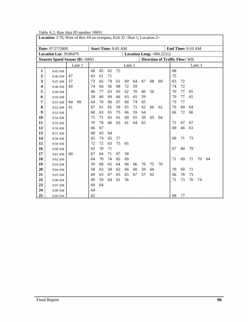
Final Report 96

Table A.2. Raw data ID number 10691. Location: I-70, West of Box #4 on overpass, Exit 32 <Run 1, Location 2>

Date: 07/27/2009 Start Time: 8:45 AM End Time: 9:10 AM Location Lat: 39.86479 Location Long: -084.22312 Nearest Speed Sensor ID: 10691 Direction of Traffic Flow: WB Lane 1 Lane 2 Lane 3

1 8:45 AM 68 65 65 72 68 2 8:46 AM 67 63 61 71 75 3 8:47 AM 57 72 65 74 61 69 64 67 68 69 63 72 4 8:48 AM 69 74 64 56 68 72 59 74 72 5 8:49 AM 66 77 63 65 62 70 60 56 70 77 65 6 8:50 AM 58 66 69 66 63 65 59 70 77 65 7 8:51 AM 64 69 64 70 66 67 68 74 65 73 77 8 8:52 AM 61 67 61 65 59 65 71 62 66 62 70 69 64 9 8:53 AM 68 63 65 75 66 59 64 66 72 66

10 8:54 AM 75 71 63 61 69 65 58 65 64 11 8:55 AM 70 70 66 63 61 64 65 71 67 67 12 8:56 AM 66 67 69 46 63 13 8:57 AM 68 63 64 14 8:58 AM 65 74 65 57 69 71 73 15 8:59 AM 72 72 63 75 65 16 9:00 AM 63 70 71 67 80 79 17 9:01 AM 60 67 64 71 67 58 18 9:02 AM 64 70 74 65 69 71 69 71 70 64 19 9:03 AM 59 68 65 64 66 66 76 75 70 20 9:04 AM 58 63 58 62 66 60 59 66 70 69 71 21 9:05 AM 69 63 67 65 65 67 57 62 66 78 73 22 9:06 AM 60 59 64 61 56 71 73 70 74 23 9:07 AM 68 64 24 9:08 AM 64 25 9:09 AM 62 68 77

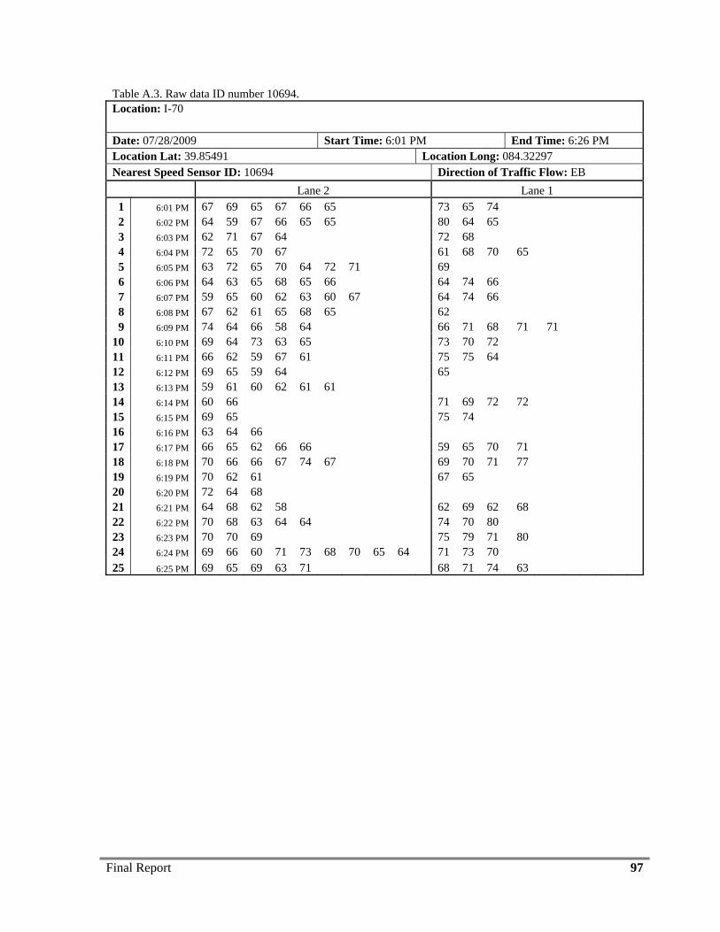
Final Report 97

Table A.3. Raw data ID number 10694. Location: I-70

Date: 07/28/2009 Start Time: 6:01 PM End Time: 6:26 PM Location Lat: 39.85491 Location Long: 084.32297 Nearest Speed Sensor ID: 10694 Direction of Traffic Flow: EB Lane 2 Lane 1

1 6:01 PM 67 69 65 67 66 65 73 65 74 2 6:02 PM 64 59 67 66 65 65 80 64 65 3 6:03 PM 62 71 67 64 72 68 4 6:04 PM 72 65 70 67 61 68 70 65 5 6:05 PM 63 72 65 70 64 72 71 69 6 6:06 PM 64 63 65 68 65 66 64 74 66 7 6:07 PM 59 65 60 62 63 60 67 64 74 66 8 6:08 PM 67 62 61 65 68 65 62 9 6:09 PM 74 64 66 58 64 66 71 68 71 71

10 6:10 PM 69 64 73 63 65 73 70 72 11 6:11 PM 66 62 59 67 61 75 75 64 12 6:12 PM 69 65 59 64 65 13 6:13 PM 59 61 60 62 61 61 14 6:14 PM 60 66 71 69 72 72 15 6:15 PM 69 65 75 74 16 6:16 PM 63 64 66 17 6:17 PM 66 65 62 66 66 59 65 70 71 18 6:18 PM 70 66 66 67 74 67 69 70 71 77 19 6:19 PM 70 62 61 67 65 20 6:20 PM 72 64 68 21 6:21 PM 64 68 62 58 62 69 62 68 22 6:22 PM 70 68 63 64 64 74 70 80 23 6:23 PM 70 70 69 75 79 71 80 24 6:24 PM 69 66 60 71 73 68 70 65 64 71 73 70 25 6:25 PM 69 65 69 63 71 68 71 74 63

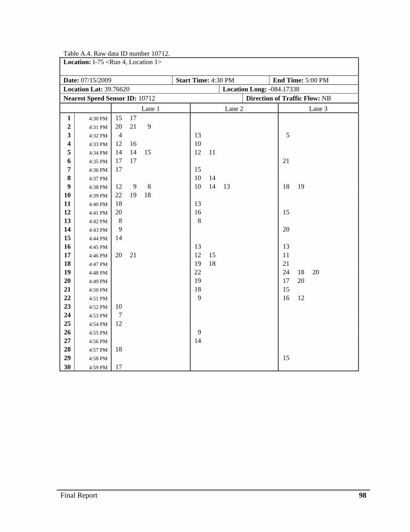
Final Report 98

Table A.4. Raw data ID number 10712. Location: I-75 <Run 4, Location 1>

Date: 07/15/2009 Start Time: 4:30 PM End Time: 5:00 PM Location Lat: 39.76620 Location Long: -084.17338 Nearest Speed Sensor ID: 10712 Direction of Traffic Flow: NB Lane 1 Lane 2 Lane 3

1 4:30 PM 15 17 2 4:31 PM 20 21 9 3 4:32 PM 4 13 5 4 4:33 PM 12 16 10 5 4:34 PM 14 14 15 12 11 6 4:35 PM 17 17 21 7 4:36 PM 17 15 8 4:37 PM 10 14 9 4:38 PM 12 9 8 10 14 13 18 19

10 4:39 PM 22 19 18 11 4:40 PM 18 13 12 4:41 PM 20 16 15 13 4:42 PM 8 8 14 4:43 PM 9 20 15 4:44 PM 14 16 4:45 PM 13 13 17 4:46 PM 20 21 12 15 11 18 4:47 PM 19 18 21 19 4:48 PM 22 24 18 20 20 4:49 PM 19 17 20 21 4:50 PM 18 15 22 4:51 PM 9 16 12 23 4:52 PM 10 24 4:53 PM 7 25 4:54 PM 12 26 4:55 PM 9 27 4:56 PM 14 28 4:57 PM 18 29 4:58 PM 15 30 4:59 PM 17

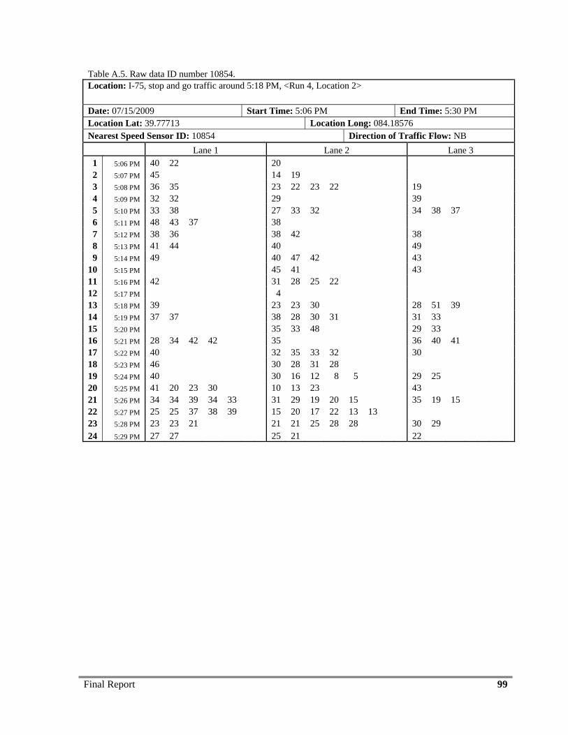
Final Report 99

Table A.5. Raw data ID number 10854. Location: I-75, stop and go traffic around 5:18 PM, <Run 4, Location 2>

Date: 07/15/2009 Start Time: 5:06 PM End Time: 5:30 PM Location Lat: 39.77713 Location Long: 084.18576 Nearest Speed Sensor ID: 10854 Direction of Traffic Flow: NB Lane 1 Lane 2 Lane 3

1 5:06 PM 40 22 20 2 5:07 PM 45 14 19 3 5:08 PM 36 35 23 22 23 22 19 4 5:09 PM 32 32 29 39 5 5:10 PM 33 38 27 33 32 34 38 37 6 5:11 PM 48 43 37 38 7 5:12 PM 38 36 38 42 38 8 5:13 PM 41 44 40 49 9 5:14 PM 49 40 47 42 43

10 5:15 PM 45 41 43 11 5:16 PM 42 31 28 25 22 12 5:17 PM 4 13 5:18 PM 39 23 23 30 28 51 39 14 5:19 PM 37 37 38 28 30 31 31 33 15 5:20 PM 35 33 48 29 33 16 5:21 PM 28 34 42 42 35 36 40 41 17 5:22 PM 40 32 35 33 32 30 18 5:23 PM 46 30 28 31 28 19 5:24 PM 40 30 16 12 8 5 29 25 20 5:25 PM 41 20 23 30 10 13 23 43 21 5:26 PM 34 34 39 34 33 31 29 19 20 15 35 19 15 22 5:27 PM 25 25 37 38 39 15 20 17 22 13 13 23 5:28 PM 23 23 21 21 21 25 28 28 30 29 24 5:29 PM 27 27 25 21 22

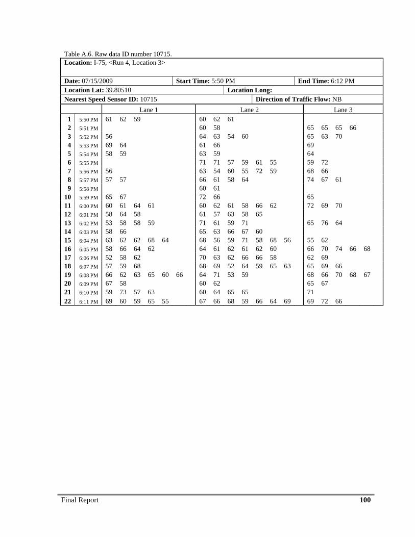
Final Report 100

Table A.6. Raw data ID number 10715. Location: I-75, <Run 4, Location 3>

Date: 07/15/2009 Start Time: 5:50 PM End Time: 6:12 PM Location Lat: 39.80510 Location Long: Nearest Speed Sensor ID: 10715 Direction of Traffic Flow: NB Lane 1 Lane 2 Lane 3

1 5:50 PM 61 62 59 60 62 61 2 5:51 PM 60 58 65 65 65 66 3 5:52 PM 56 64 63 54 60 65 63 70 4 5:53 PM 69 64 61 66 69 5 5:54 PM 58 59 63 59 64 6 5:55 PM 71 71 57 59 61 55 59 72 7 5:56 PM 56 63 54 60 55 72 59 68 66 8 5:57 PM 57 57 66 61 58 64 74 67 61 9 5:58 PM 60 61

10 5:59 PM 65 67 72 66 65 11 6:00 PM 60 61 64 61 60 62 61 58 66 62 72 69 70 12 6:01 PM 58 64 58 61 57 63 58 65 13 6:02 PM 53 58 58 59 71 61 59 71 65 76 64 14 6:03 PM 58 66 65 63 66 67 60 15 6:04 PM 63 62 62 68 64 68 56 59 71 58 68 56 55 62 16 6:05 PM 58 66 64 62 64 61 62 61 62 60 66 70 74 66 68 17 6:06 PM 52 58 62 70 63 62 66 66 58 62 69 18 6:07 PM 57 59 68 68 69 52 64 59 65 63 65 69 66 19 6:08 PM 66 62 63 65 60 66 64 71 53 59 68 66 70 68 67 20 6:09 PM 67 58 60 62 65 67 21 6:10 PM 59 73 57 63 60 64 65 65 71 22 6:11 PM 69 60 59 65 55 67 66 68 59 66 64 69 69 72 66

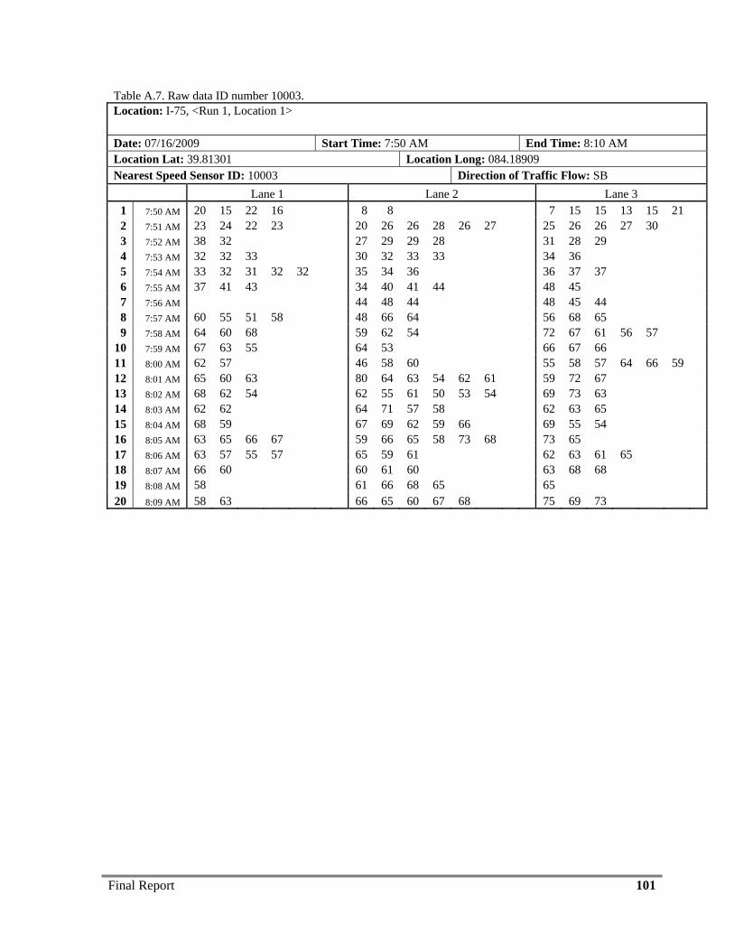
Final Report 101


Date: 07/16/2009 Start Time: 7:50 AM End Time: 8:10 AM Location Lat: 39.81301 Location Long: 084.18909 Nearest Speed Sensor ID: 10003 Direction of Traffic Flow: SB Lane 1 Lane 2 Lane 3

1 7:50 AM 20 15 22 16 8 8 7 15 15 13 15 21 2 7:51 AM 23 24 22 23 20 26 26 28 26 27 25 26 26 27 30 3 7:52 AM 38 32 27 29 29 28 31 28 29 4 7:53 AM 32 32 33 30 32 33 33 34 36 5 7:54 AM 33 32 31 32 32 35 34 36 36 37 37 6 7:55 AM 37 41 43 34 40 41 44 48 45 7 7:56 AM 44 48 44 48 45 44 8 7:57 AM 60 55 51 58 48 66 64 56 68 65 9 7:58 AM 64 60 68 59 62 54 72 67 61 56 57

10 7:59 AM 67 63 55 64 53 66 67 66 11 8:00 AM 62 57 46 58 60 55 58 57 64 66 59 12 8:01 AM 65 60 63 80 64 63 54 62 61 59 72 67 13 8:02 AM 68 62 54 62 55 61 50 53 54 69 73 63 14 8:03 AM 62 62 64 71 57 58 62 63 65 15 8:04 AM 68 59 67 69 62 59 66 69 55 54 16 8:05 AM 63 65 66 67 59 66 65 58 73 68 73 65 17 8:06 AM 63 57 55 57 65 59 61 62 63 61 65 18 8:07 AM 66 60 60 61 60 63 68 68 19 8:08 AM 58 61 66 68 65 65 20 8:09 AM 58 63 66 65 60 67 68 75 69 73

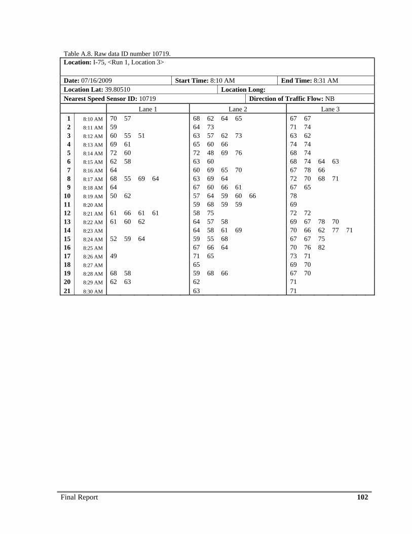
Final Report 102


Date: 07/16/2009 Start Time: 8:10 AM End Time: 8:31 AM Location Lat: 39.80510 Location Long: Nearest Speed Sensor ID: 10719 Direction of Traffic Flow: NB Lane 1 Lane 2 Lane 3

1 8:10 AM 70 57 68 62 64 65 67 67 2 8:11 AM 59 64 73 71 74 3 8:12 AM 60 55 51 63 57 62 73 63 62 4 8:13 AM 69 61 65 60 66 74 74 5 8:14 AM 72 60 72 48 69 76 68 74 6 8:15 AM 62 58 63 60 68 74 64 63 7 8:16 AM 64 60 69 65 70 67 78 66 8 8:17 AM 68 55 69 64 63 69 64 72 70 68 71 9 8:18 AM 64 67 60 66 61 67 65

10 8:19 AM 50 62 57 64 59 60 66 78 11 8:20 AM 59 68 59 59 69 12 8:21 AM 61 66 61 61 58 75 72 72 13 8:22 AM 61 60 62 64 57 58 69 67 78 70 14 8:23 AM 64 58 61 69 70 66 62 77 71 15 8:24 AM 52 59 64 59 55 68 67 67 75 16 8:25 AM 67 66 64 70 76 82 17 8:26 AM 49 71 65 73 71 18 8:27 AM 65 69 70 19 8:28 AM 68 58 59 68 66 67 70 20 8:29 AM 62 63 62 71 21 8:30 AM 63 71

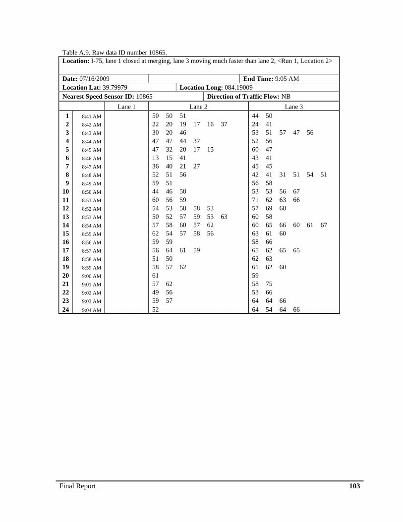
Final Report 103

Table A.9. Raw data ID number 10865. Location: I-75, lane 1 closed at merging, lane 3 moving much faster than lane 2, <Run 1, Location 2>

Date: 07/16/2009 End Time: 9:05 AM Location Lat: 39.79979 Location Long: 084.19009 Nearest Speed Sensor ID: 10865 Direction of Traffic Flow: NB Lane 1 Lane 2 Lane 3

1 8:41 AM 50 50 51 44 50 2 8:42 AM 22 20 19 17 16 37 24 41 3 8:43 AM 30 20 46 53 51 57 47 56 4 8:44 AM 47 47 44 37 52 56 5 8:45 AM 47 32 20 17 15 60 47 6 8:46 AM 13 15 41 43 41 7 8:47 AM 36 40 21 27 45 45 8 8:48 AM 52 51 56 42 41 31 51 54 51 9 8:49 AM 59 51 56 58

10 8:50 AM 44 46 58 53 53 56 67 11 8:51 AM 60 56 59 71 62 63 66 12 8:52 AM 54 53 58 58 53 57 69 68 13 8:53 AM 50 52 57 59 53 63 60 58 14 8:54 AM 57 58 60 57 62 60 65 66 60 61 67 15 8:55 AM 62 54 57 58 56 63 61 60 16 8:56 AM 59 59 58 66 17 8:57 AM 56 64 61 59 65 62 65 65 18 8:58 AM 51 50 62 63 19 8:59 AM 58 57 62 61 62 60 20 9:00 AM 61 59 21 9:01 AM 57 62 58 75 22 9:02 AM 49 56 53 66 23 9:03 AM 59 57 64 64 66 24 9:04 AM 52 64 54 64 66

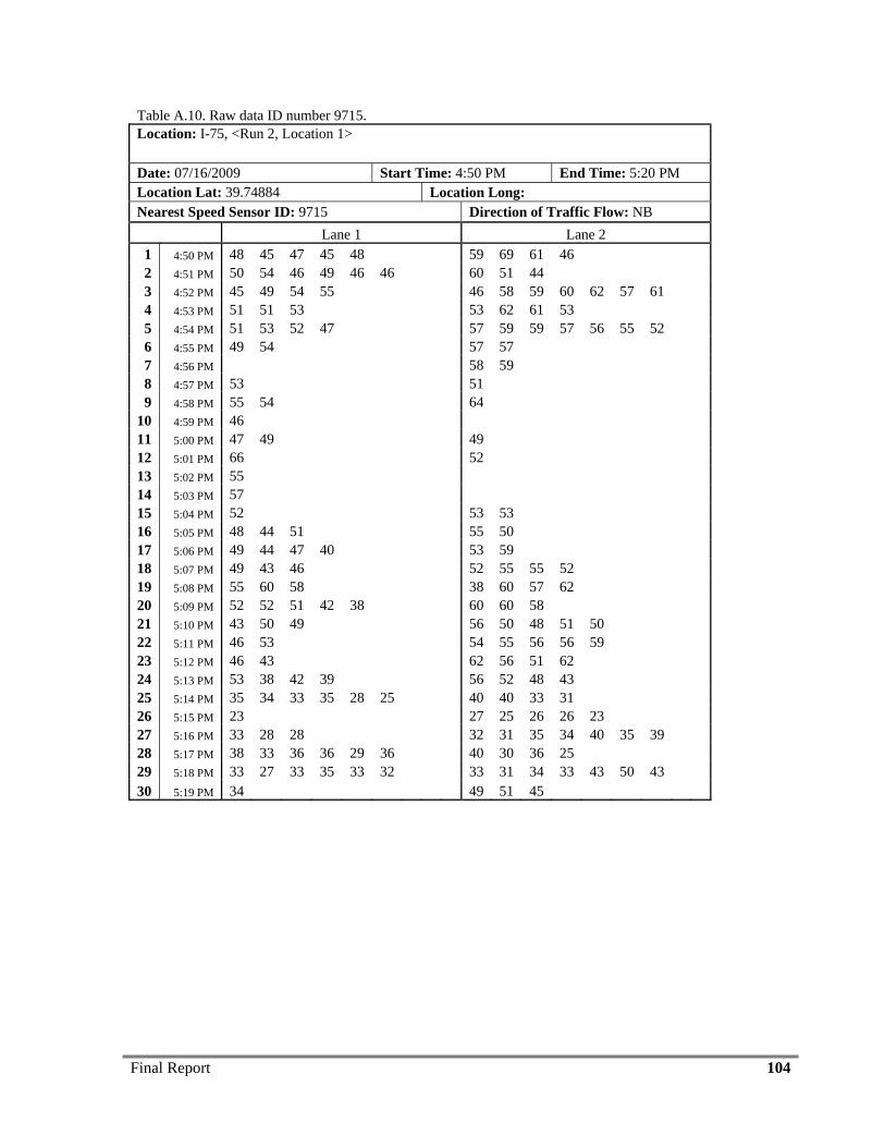
Final Report 104


Date: 07/16/2009 Start Time: 4:50 PM End Time: 5:20 PM Location Lat: 39.74884 Location Long: Nearest Speed Sensor ID: 9715 Direction of Traffic Flow: NB Lane 1 Lane 2

1 4:50 PM 48 45 47 45 48 59 69 61 46 2 4:51 PM 50 54 46 49 46 46 60 51 44 3 4:52 PM 45 49 54 55 46 58 59 60 62 57 61 4 4:53 PM 51 51 53 53 62 61 53 5 4:54 PM 51 53 52 47 57 59 59 57 56 55 52 6 4:55 PM 49 54 57 57 7 4:56 PM 58 59 8 4:57 PM 53 51 9 4:58 PM 55 54 64

10 4:59 PM 46 11 5:00 PM 47 49 49 12 5:01 PM 66 52 13 5:02 PM 55 14 5:03 PM 57 15 5:04 PM 52 53 53 16 5:05 PM 48 44 51 55 50 17 5:06 PM 49 44 47 40 53 59 18 5:07 PM 49 43 46 52 55 55 52 19 5:08 PM 55 60 58 38 60 57 62 20 5:09 PM 52 52 51 42 38 60 60 58 21 5:10 PM 43 50 49 56 50 48 51 50 22 5:11 PM 46 53 54 55 56 56 59 23 5:12 PM 46 43 62 56 51 62 24 5:13 PM 53 38 42 39 56 52 48 43 25 5:14 PM 35 34 33 35 28 25 40 40 33 31 26 5:15 PM 23 27 25 26 26 23 27 5:16 PM 33 28 28 32 31 35 34 40 35 39 28 5:17 PM 38 33 36 36 29 36 40 30 36 25 29 5:18 PM 33 27 33 35 33 32 33 31 34 33 43 50 43 30 5:19 PM 34 49 51 45

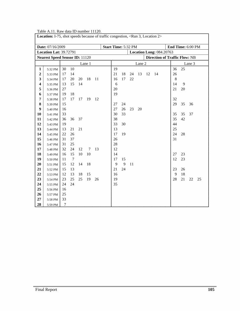
Final Report 105

Table A.11. Raw data ID number 11120. Location: I-75, shot speeds because of traffic congestion, <Run 3, Location 2>


1 5:32 PM 30 10 19 36 25 2 5:33 PM 17 14 21 18 24 13 12 14 26 3 5:34 PM 17 20 20 18 11 16 17 22 8 4 5:35 PM 13 15 14 6 14 9 5 5:36 PM 27 20 21 20 6 5:37 PM 19 18 19 7 5:38 PM 17 17 17 19 12 32 8 5:39 PM 15 27 24 29 35 36 9 5:40 PM 16 27 26 23 20

10 5:41 PM 33 30 33 35 35 37 11 5:42 PM 36 36 37 38 35 42 12 5:43 PM 19 33 30 44 13 5:44 PM 13 21 21 13 25 14 5:45 PM 22 26 17 19 24 28 15 5:46 PM 31 37 26 31 16 5:47 PM 31 25 28 17 5:48 PM 32 24 12 7 13 12 18 5:49 PM 16 15 10 10 14 27 23 19 5:50 PM 11 7 17 15 12 23 20 5:51 PM 15 12 14 18 9 9 11 21 5:52 PM 15 13 21 24 23 26 22 5:53 PM 12 13 18 15 16 9 18 23 5:54 PM 23 25 25 19 26 19 28 21 22 25 24 5:55 PM 24 24 35 25 5:56 PM 16 26 5:57 PM 25 27 5:58 PM 33 28 5:59 PM 7

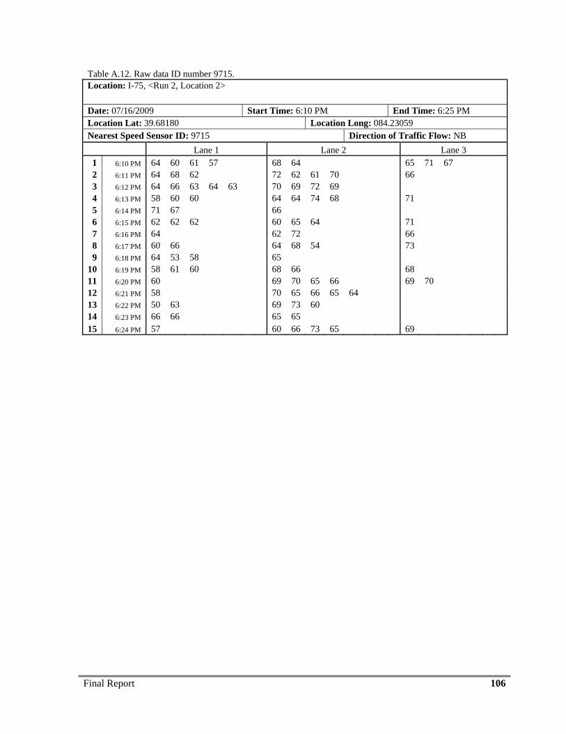
Final Report 106



1 6:10 PM 64 60 61 57 68 64 65 71 67 2 6:11 PM 64 68 62 72 62 61 70 66 3 6:12 PM 64 66 63 64 63 70 69 72 69 4 6:13 PM 58 60 60 64 64 74 68 71 5 6:14 PM 71 67 66 6 6:15 PM 62 62 62 60 65 64 71 7 6:16 PM 64 62 72 66 8 6:17 PM 60 66 64 68 54 73 9 6:18 PM 64 53 58 65

10 6:19 PM 58 61 60 68 66 68 11 6:20 PM 60 69 70 65 66 69 70 12 6:21 PM 58 70 65 66 65 64 13 6:22 PM 50 63 69 73 60 14 6:23 PM 66 66 65 65 15 6:24 PM 57 60 66 73 65 69

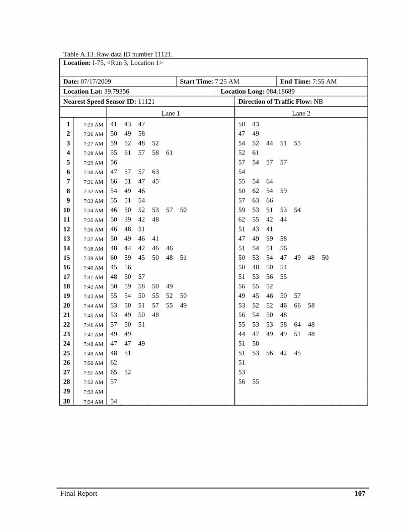
Final Report 107


Date: 07/17/2009 Start Time: 7:25 AM End Time: 7:55 AM Location Lat: 39.79356 Location Long: 084.18689 Nearest Speed Sensor ID: 11121 Direction of Traffic Flow: NB

Lane 1 Lane 2 1 7:25 AM 41 43 47 50 43 2 7:26 AM 50 49 58 47 49 3 7:27 AM 59 52 48 52 54 52 44 51 55 4 7:28 AM 55 61 57 58 61 52 61 5 7:29 AM 56 57 54 57 57 6 7:30 AM 47 57 57 63 54 7 7:31 AM 66 51 47 45 55 54 64 8 7:32 AM 54 49 46 50 62 54 59 9 7:33 AM 55 51 54 57 63 66

10 7:34 AM 46 50 52 53 57 50 59 53 51 53 54 11 7:35 AM 50 39 42 48 62 55 42 44 12 7:36 AM 46 48 51 51 43 41 13 7:37 AM 50 49 46 41 47 49 59 58 14 7:38 AM 48 44 42 46 46 51 54 51 56 15 7:39 AM 60 59 45 50 48 51 50 53 54 47 49 48 50 16 7:40 AM 45 56 50 48 50 54 17 7:41 AM 48 50 57 51 53 56 55 18 7:42 AM 50 59 58 50 49 56 55 52 19 7:43 AM 55 54 50 55 52 50 49 45 46 50 57 20 7:44 AM 53 50 51 57 55 49 53 52 52 46 66 58 21 7:45 AM 53 49 50 48 56 54 50 48 22 7:46 AM 57 50 51 55 53 53 58 64 48 23 7:47 AM 49 49 44 47 49 49 51 48 24 7:48 AM 47 47 49 51 50 25 7:49 AM 48 51 51 53 56 42 45 26 7:50 AM 62 51 27 7:51 AM 65 52 53 28 7:52 AM 57 56 55 29 7:53 AM 30 7:54 AM 54

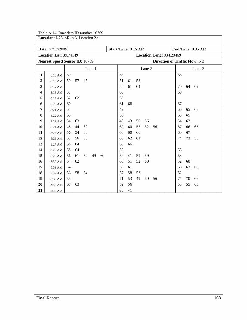
Final Report 108


Date: 07/17/2009 Start Time: 8:15 AM End Time: 8:35 AM Location Lat: 39.74149 Location Long: 084.20469 Nearest Speed Sensor ID: 10709 Direction of Traffic Flow: NB

Lane 1 Lane 2 Lane 3 1 8:15 AM 59 53 65 2 8:16 AM 59 57 45 51 61 53 3 8:17 AM 56 61 64 70 64 69 4 8:18 AM 52 63 69 5 8:19 AM 62 62 66 6 8:20 AM 60 61 66 67 7 8:21 AM 61 49 66 65 68 8 8:22 AM 63 56 63 65 9 8:23 AM 54 63 40 43 50 56 54 62

10 8:24 AM 48 44 62 62 60 55 52 56 67 66 63 11 8:25 AM 56 54 63 60 60 66 60 67 12 8:26 AM 65 56 55 60 62 63 74 72 58 13 8:27 AM 58 64 68 66 14 8:28 AM 68 64 55 66 15 8:29 AM 56 61 54 49 60 59 41 59 59 53 16 8:30 AM 64 62 60 51 52 60 52 60 17 8:31 AM 54 63 61 68 63 65 18 8:32 AM 56 58 54 57 58 53 62 19 8:33 AM 55 71 53 49 50 56 74 70 66 20 8:34 AM 67 63 52 56 58 55 63 21 8:35 AM 60 41

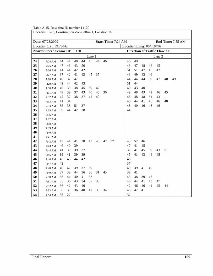
Final Report 109

Table A.15. Raw data ID number 11120. Location: I-75, Construction Zone <Run 1, Location 1>

Date: 07/28/2009 Start Time: 7:24 AM End Time: 7:55 AM Location Lat: 39.79042 Location Long: 084.18496 Nearest Speed Sensor ID: 11120 Direction of Traffic Flow: SB Lane 1 Lane 2 24 7:24 AM 44 44 48 44 45 44 46 46 49 25 7:25 AM 47 46 43 56 48 47 48 46 45 26 7:26 AM 41 44 42 42 51 51 47 45 42 27 7:27 AM 37 42 41 42 45 37 48 49 43 46 28 7:28 AM 40 37 47 44 44 44 39 47 40 49 29 7:29 AM 42 44 42 43 51 44 30 7:30 AM 40 39 38 45 39 42 40 43 40 31 7:31 AM 49 39 37 43 40 46 36 49 48 43 41 46 45 32 7:32 AM 42 37 38 37 42 40 45 48 48 51 43 33 7:33 AM 41 34 40 44 41 46 46 40 34 7:34 AM 35 38 51 37 48 40 46 48 46 35 7:35 AM 39 44 42 38 44 36 7:36 AM 37 7:37 AM 38 7:38 AM 39 7:39 AM 40 7:40 AM 41 7:41 AM 42 7:42 AM 43 44 41 38 43 48 47 37 43 52 46 43 7:43 AM 46 40 39 47 41 45 44 7:44 AM 41 39 39 37 39 41 45 39 43 51 45 7:45 AM 39 41 39 39 45 41 43 44 45 46 7:46 AM 45 45 44 42 46 47 7:47 AM 42 37 48 7:48 AM 40 42 39 37 39 40 39 41 40 49 7:49 AM 37 39 44 36 36 31 45 39 41 50 7:50 AM 38 44 40 41 38 43 38 39 45 51 7:51 AM 35 36 43 34 37 39 45 44 41 43 47 52 7:52 AM 36 42 43 40 42 46 46 41 45 44 53 7:53 AM 36 39 36 40 42 35 34 48 47 41 54 7:54 AM 38 27 37

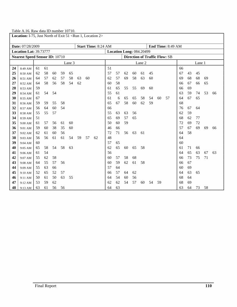
Final Report 110

Table A.16. Raw data ID number 10710. Location: I-75, Just North of Exit 51 <Run 1, Location 2>

Date: 07/28/2009 Start Time: 8:24 AM End Time: 8:49 AM Location Lat: 39.73777 Location Long: 084.20499 Nearest Speed Sensor ID: 10710 Direction of Traffic Flow: SB Lane 3 Lane 2 Lane 1 24 8:49 AM 61 61 51 66 25 8:50 AM 62 58 60 59 65 57 57 62 60 61 45 67 43 45 26 8:51 AM 64 57 62 57 58 63 60 62 57 69 58 63 60 69 68 68 69 27 8:52 AM 64 58 56 58 54 62 60 58 66 67 66 65 28 8:53 AM 59 61 65 55 55 69 60 66 69 29 8:54 AM 61 54 54 55 61 63 59 74 53 66 30 8:55 AM 67 61 6 65 65 58 54 60 57 64 67 65 31 8:56 AM 59 59 55 58 65 67 58 60 62 59 68 32 8:57 AM 56 64 60 54 66 76 67 64 33 8:58 AM 55 55 57 55 63 63 56 62 59 34 8:59 AM 51 65 69 57 65 68 62 77 35 9:00 AM 61 57 56 61 60 50 60 59 72 69 72 36 9:01 AM 59 60 38 35 60 46 66 57 67 69 69 66 37 9:02 AM 62 61 60 56 72 71 56 63 61 64 58 38 9:03 AM 56 56 61 61 54 59 57 62 48 64 39 9:04 AM 60 57 65 60 40 9:05 AM 65 58 54 58 63 62 65 60 65 58 61 71 66 41 9:06 AM 61 54 56 64 65 63 67 63 42 9:07 AM 55 62 58 60 57 58 68 66 73 75 71 43 9:08 AM 64 55 57 56 60 59 62 61 58 66 67 44 9:09 AM 55 63 66 57 64 60 69 45 9:10 AM 52 65 52 57 66 57 64 62 64 63 65 46 9:11 AM 50 61 50 63 55 64 54 60 56 68 64 47 9:12 AM 53 59 62 62 62 54 57 60 54 59 68 69 48 9:13 AM 63 61 56 56 64 63 63 64 73 58

Final Report 111


Date: 08/17/2009 Start Time: 8:25 AM End Time: 8:50 AM Location Lat: 39.77002 Location Long: 084.08743 Nearest Speed Sensor ID: 10791 Direction of Traffic Flow: SB Lane 1 Lane 2 Lane 3 31 8:25 AM 64 67 67 68 64 66 71 66 73 72 32 8:26 AM 73 67 69 73 73 73 33 8:27 AM 65 65 67 76 72 63 69 75 74 34 8:28 AM 71 67 65 67 62 75 35 8:29 AM 66 67 69 71 77 77 36 8:30 AM 65 75 69 77 66 75 69 66 78 69 37 8:31 AM 69 75 72 73 69 76 72 78 74 38 8:32 AM 61 67 65 73 71 69 65 39 8:33 AM 66 64 66 78 68 66 66 72 71 77 68 72 76 40 8:34 AM 71 75 68 65 77 62 68 69 41 8:35 AM 67 73 70 75 67 65 69 75 42 8:36 AM 71 71 72 55 70 70 76 43 8:37 AM 68 69 67 68 65 74 71 44 8:38 AM 67 54 67 69 72 73 66 70 68 74 71 45 8:39 AM 66 62 67 63 64 76 77 46 8:40 AM 68 60 69 69 71 67 83 74 47 8:41 AM 67 66 74 68 70 65 74 48 8:42 AM 64 63 73 63 65 65 70 75 72 67 66 49 8:43 AM 57 70 73 68 67 73 70 66 73 50 8:44 AM 67 76 74 73 77 72 75 51 8:45 AM 60 66 52 8:46 AM 60 68 63 69 71 74 53 8:47 AM 65 65 67 62 61 76 72 54 8:48 AM 64 54 71 65 68 69 67 66 70 76 55 8:49 AM 69 68 69 66 62 69 65 70 65 74 69

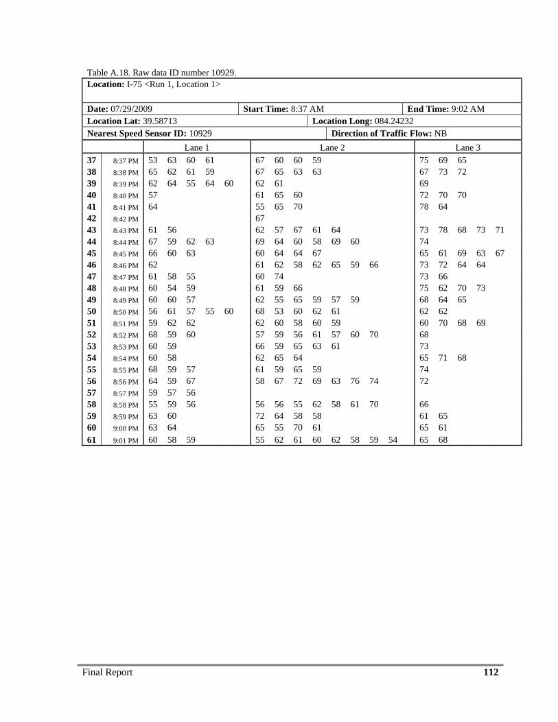
Final Report 112


Date: 07/29/2009 Start Time: 8:37 AM End Time: 9:02 AM Location Lat: 39.58713 Location Long: 084.24232 Nearest Speed Sensor ID: 10929 Direction of Traffic Flow: NB Lane 1 Lane 2 Lane 3 37 8:37 PM 53 63 60 61 67 60 60 59 75 69 65 38 8:38 PM 65 62 61 59 67 65 63 63 67 73 72 39 8:39 PM 62 64 55 64 60 62 61 69 40 8:40 PM 57 61 65 60 72 70 70 41 8:41 PM 64 55 65 70 78 64 42 8:42 PM 67 43 8:43 PM 61 56 62 57 67 61 64 73 78 68 73 71 44 8:44 PM 67 59 62 63 69 64 60 58 69 60 74 45 8:45 PM 66 60 63 60 64 64 67 65 61 69 63 67 46 8:46 PM 62 61 62 58 62 65 59 66 73 72 64 64 47 8:47 PM 61 58 55 60 74 73 66 48 8:48 PM 60 54 59 61 59 66 75 62 70 73 49 8:49 PM 60 60 57 62 55 65 59 57 59 68 64 65 50 8:50 PM 56 61 57 55 60 68 53 60 62 61 62 62 51 8:51 PM 59 62 62 62 60 58 60 59 60 70 68 69 52 8:52 PM 68 59 60 57 59 56 61 57 60 70 68 53 8:53 PM 60 59 66 59 65 63 61 73 54 8:54 PM 60 58 62 65 64 65 71 68 55 8:55 PM 68 59 57 61 59 65 59 74 56 8:56 PM 64 59 67 58 67 72 69 63 76 74 72 57 8:57 PM 59 57 56 58 8:58 PM 55 59 56 56 56 55 62 58 61 70 66 59 8:59 PM 63 60 72 64 58 58 61 65 60 9:00 PM 63 64 65 55 70 61 65 61 61 9:01 PM 60 58 59 55 62 61 60 62 58 59 54 65 68

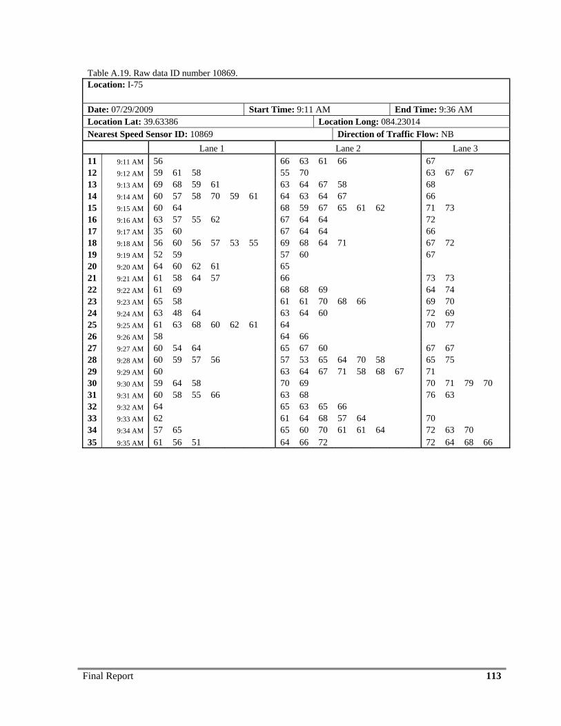
Final Report 113


Date: 07/29/2009 Start Time: 9:11 AM End Time: 9:36 AM Location Lat: 39.63386 Location Long: 084.23014 Nearest Speed Sensor ID: 10869 Direction of Traffic Flow: NB Lane 1 Lane 2 Lane 3 11 9:11 AM 56 66 63 61 66 67 12 9:12 AM 59 61 58 55 70 63 67 67 13 9:13 AM 69 68 59 61 63 64 67 58 68 14 9:14 AM 60 57 58 70 59 61 64 63 64 67 66 15 9:15 AM 60 64 68 59 67 65 61 62 71 73 16 9:16 AM 63 57 55 62 67 64 64 72 17 9:17 AM 35 60 67 64 64 66 18 9:18 AM 56 60 56 57 53 55 69 68 64 71 67 72 19 9:19 AM 52 59 57 60 67 20 9:20 AM 64 60 62 61 65 21 9:21 AM 61 58 64 57 66 73 73 22 9:22 AM 61 69 68 68 69 64 74 23 9:23 AM 65 58 61 61 70 68 66 69 70 24 9:24 AM 63 48 64 63 64 60 72 69 25 9:25 AM 61 63 68 60 62 61 64 70 77 26 9:26 AM 58 64 66 27 9:27 AM 60 54 64 65 67 60 67 67 28 9:28 AM 60 59 57 56 57 53 65 64 70 58 65 75 29 9:29 AM 60 63 64 67 71 58 68 67 71 30 9:30 AM 59 64 58 70 69 70 71 79 70 31 9:31 AM 60 58 55 66 63 68 76 63 32 9:32 AM 64 65 63 65 66 33 9:33 AM 62 61 64 68 57 64 70 34 9:34 AM 57 65 65 60 70 61 61 64 72 63 70 35 9:35 AM 61 56 51 64 66 72 72 64 68 66

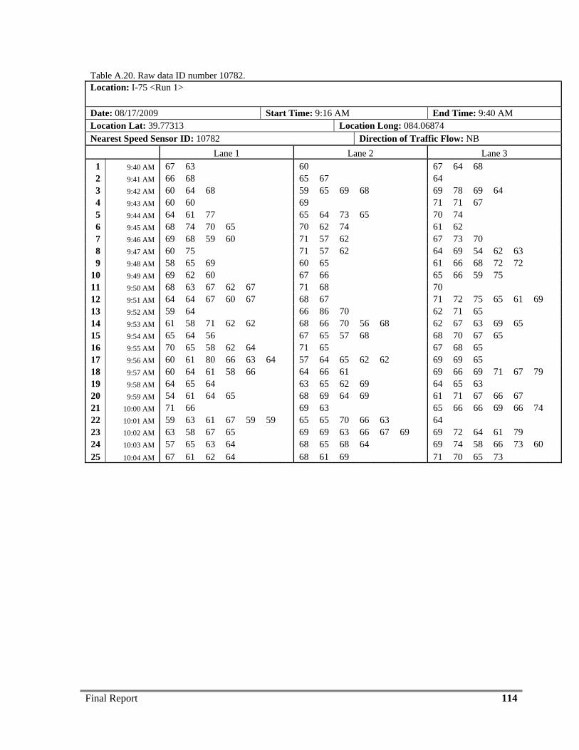
Final Report 114

Table A.20. Raw data ID number 10782. Location: I-75 <Run 1>

Date: 08/17/2009 Start Time: 9:16 AM End Time: 9:40 AM Location Lat: 39.77313 Location Long: 084.06874 Nearest Speed Sensor ID: 10782 Direction of Traffic Flow: NB Lane 1 Lane 2 Lane 3

1 9:40 AM 67 63 60 67 64 68 2 9:41 AM 66 68 65 67 64 3 9:42 AM 60 64 68 59 65 69 68 69 78 69 64 4 9:43 AM 60 60 69 71 71 67 5 9:44 AM 64 61 77 65 64 73 65 70 74 6 9:45 AM 68 74 70 65 70 62 74 61 62 7 9:46 AM 69 68 59 60 71 57 62 67 73 70 8 9:47 AM 60 75 71 57 62 64 69 54 62 63 9 9:48 AM 58 65 69 60 65 61 66 68 72 72

10 9:49 AM 69 62 60 67 66 65 66 59 75 11 9:50 AM 68 63 67 62 67 71 68 70 12 9:51 AM 64 64 67 60 67 68 67 71 72 75 65 61 69 13 9:52 AM 59 64 66 86 70 62 71 65 14 9:53 AM 61 58 71 62 62 68 66 70 56 68 62 67 63 69 65 15 9:54 AM 65 64 56 67 65 57 68 68 70 67 65 16 9:55 AM 70 65 58 62 64 71 65 67 68 65 17 9:56 AM 60 61 80 66 63 64 57 64 65 62 62 69 69 65 18 9:57 AM 60 64 61 58 66 64 66 61 69 66 69 71 67 79 19 9:58 AM 64 65 64 63 65 62 69 64 65 63 20 9:59 AM 54 61 64 65 68 69 64 69 61 71 67 66 67 21 10:00 AM 71 66 69 63 65 66 66 69 66 74 22 10:01 AM 59 63 61 67 59 59 65 65 70 66 63 64 23 10:02 AM 63 58 67 65 69 69 63 66 67 69 69 72 64 61 79 24 10:03 AM 57 65 63 64 68 65 68 64 69 74 58 66 73 60 25 10:04 AM 67 61 62 64 68 61 69 71 70 65 73

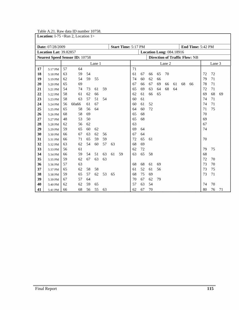
Final Report 115


Date: 07/28/2009 Start Time: 5:17 PM End Time: 5:42 PM Location Lat: 39.82857 Location Long: 084.18916 Nearest Speed Sensor ID: 10758 Direction of Traffic Flow: NB Lane 1 Lane 2 Lane 3 17 5:17 PM 57 64 71 18 5:18 PM 63 59 54 61 67 66 65 70 72 72 19 5:19 PM 62 54 59 55 74 60 62 66 79 71 20 5:20 PM 65 69 67 66 67 69 66 61 68 66 78 71 21 5:21 PM 54 74 73 61 59 65 69 63 64 68 64 72 71 22 5:22 PM 58 61 62 66 62 61 66 65 69 68 69 23 5:23 PM 58 63 57 51 54 60 61 74 71 24 5:24 PM 56 60a66 61 67 60 61 52 74 71 25 5:25 PM 65 58 56 64 64 60 72 71 75 26 5:26 PM 68 58 69 65 68 70 27 5:27 PM 48 53 50 65 68 69 28 5:28 PM 62 56 62 63 67 29 5:29 PM 59 65 60 62 69 64 74 30 5:30 PM 66 67 63 62 56 67 64 31 5:31 PM 66 71 65 59 59 72 65 61 70 32 5:32 PM 63 62 54 60 57 63 68 69 33 5:33 PM 56 61 62 72 79 75 34 5:34 PM 66 59 54 51 63 61 59 63 65 58 68 35 5:35 PM 59 62 67 63 63 72 70 36 5:36 PM 57 63 68 68 61 69 73 70 37 5:37 PM 65 62 58 58 61 52 61 56 73 75 38 5:38 PM 59 65 57 62 53 65 68 75 69 73 71 39 5:39 PM 67 57 64 70 67 62 79 40 5:40 PM 62 62 59 65 57 63 54 74 70 41 5:41 PM 66 68 56 55 63 62 67 70 80 76 71

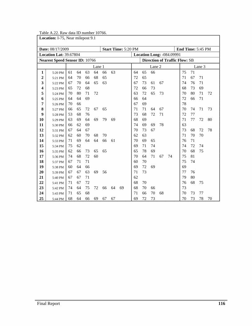
Final Report 116

Table A.22. Raw data ID number 10766. Location: I-75, Near milepost 9.1

Date: 08/17/2009 Start Time: 5:20 PM End Time: 5:45 PM Location Lat: 39.67804 Location Long: -084.09991 Nearest Speed Sensor ID: 10766 Direction of Traffic Flow: SB Lane 1 Lane 2 Lane 3

1 5:20 PM 61 64 63 64 66 63 64 65 66 75 71 2 5:21 PM 64 70 66 68 65 72 65 71 67 71 3 5:22 PM 67 70 64 65 63 67 73 61 67 74 76 71 4 5:23 PM 65 72 68 72 66 73 68 73 69 5 5:24 PM 70 80 71 72 63 72 65 73 70 80 71 72 6 5:25 PM 64 64 69 66 64 72 66 71 7 5:26 PM 70 66 67 69 78 8 5:27 PM 66 65 72 67 65 71 71 64 67 70 74 71 73 9 5:28 PM 53 68 76 73 68 72 71 72 77

10 5:29 PM 63 69 64 69 79 69 68 69 71 77 72 80 11 5:30 PM 66 62 69 74 69 69 78 63 12 5:31 PM 67 64 67 70 73 67 73 68 72 78 13 5:32 PM 62 60 70 68 70 62 63 71 70 70 14 5:33 PM 71 69 64 64 66 61 70 69 65 76 71 15 5:34 PM 75 62 69 71 74 74 72 74 16 5:35 PM 62 66 73 65 65 65 78 69 70 68 75 17 5:36 PM 74 68 72 60 70 64 71 67 74 75 81 18 5:37 PM 67 71 71 60 70 75 74 19 5:38 PM 60 64 66 69 72 69 69 20 5:39 PM 67 67 63 69 56 71 73 77 76 21 5:40 PM 67 67 71 62 79 80 22 5:41 PM 71 67 72 68 70 76 68 75 23 5:42 PM 74 64 75 72 66 64 69 68 70 66 73 24 5:43 PM 71 65 68 71 66 70 68 70 73 77 25 5:44 PM 68 64 66 69 67 67 69 72 73 70 73 78 70

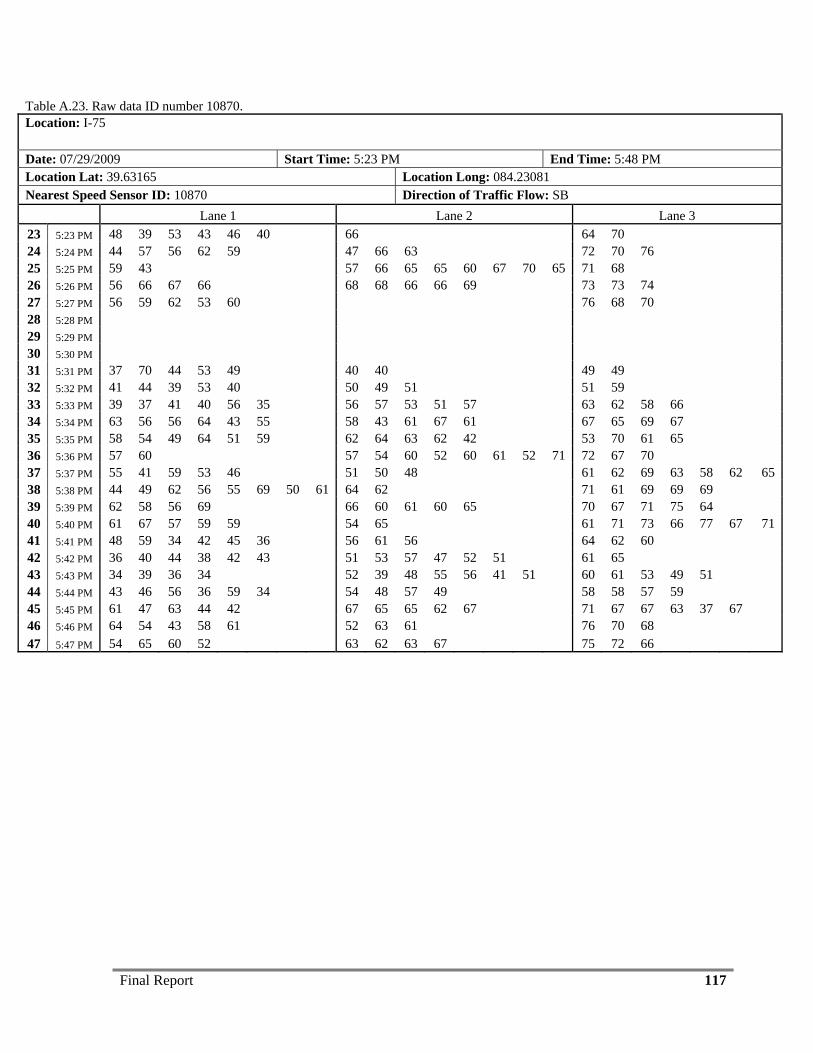
Final Report 117


Date: 07/29/2009 Start Time: 5:23 PM End Time: 5:48 PM Location Lat: 39.63165 Location Long: 084.23081 Nearest Speed Sensor ID: 10870 Direction of Traffic Flow: SB Lane 1 Lane 2 Lane 3 23 5:23 PM 48 39 53 43 46 40 66 64 70 24 5:24 PM 44 57 56 62 59 47 66 63 72 70 76 25 5:25 PM 59 43 57 66 65 65 60 67 70 65 71 68 26 5:26 PM 56 66 67 66 68 68 66 66 69 73 73 74 27 5:27 PM 56 59 62 53 60 76 68 70 28 5:28 PM 29 5:29 PM 30 5:30 PM 31 5:31 PM 37 70 44 53 49 40 40 49 49 32 5:32 PM 41 44 39 53 40 50 49 51 51 59 33 5:33 PM 39 37 41 40 56 35 56 57 53 51 57 63 62 58 66 34 5:34 PM 63 56 56 64 43 55 58 43 61 67 61 67 65 69 67 35 5:35 PM 58 54 49 64 51 59 62 64 63 62 42 53 70 61 65 36 5:36 PM 57 60 57 54 60 52 60 61 52 71 72 67 70 37 5:37 PM 55 41 59 53 46 51 50 48 61 62 69 63 58 62 6538 5:38 PM 44 49 62 56 55 69 50 61 64 62 71 61 69 69 69 39 5:39 PM 62 58 56 69 66 60 61 60 65 70 67 71 75 64 40 5:40 PM 61 67 57 59 59 54 65 61 71 73 66 77 67 7141 5:41 PM 48 59 34 42 45 36 56 61 56 64 62 60 42 5:42 PM 36 40 44 38 42 43 51 53 57 47 52 51 61 65 43 5:43 PM 34 39 36 34 52 39 48 55 56 41 51 60 61 53 49 51 44 5:44 PM 43 46 56 36 59 34 54 48 57 49 58 58 57 59 45 5:45 PM 61 47 63 44 42 67 65 65 62 67 71 67 67 63 37 67 46 5:46 PM 64 54 43 58 61 52 63 61 76 70 68 47 5:47 PM 54 65 60 52 63 62 63 67 75 72 66

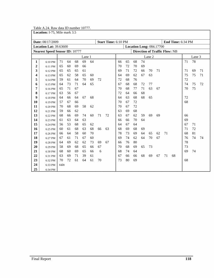
Final Report 118

Table A.24. Raw data ID number 10777. Location: I-75, Mile mark 3.5


1 6:10 PM 71 64 68 69 64 66 65 68 74 71 78 2 6:11 PM 65 60 69 66 70 72 70 69 3 6:12 PM 65 65 65 61 69 71 72 66 70 71 71 69 71 4 6:13 PM 65 62 58 65 60 64 69 62 67 63 75 75 71 5 6:14 PM 59 61 64 70 69 72 72 68 76 72 6 6:15 PM 64 73 71 64 65 67 68 68 72 77 74 75 72 7 6:16 PM 65 71 67 70 68 77 71 63 67 70 75 8 6:17 PM 63 56 67 72 64 66 68 9 6:18 PM 64 66 64 67 68 64 63 68 68 65 72

10 6:19 PM 57 67 66 70 67 72 68 11 6:20 PM 70 68 69 58 62 70 67 72 12 6:21 PM 59 66 62 63 69 68 13 6:22 PM 68 66 69 74 60 71 72 63 67 62 59 69 69 66 14 6:23 PM 61 63 64 63 66 66 70 64 69 15 6:24 PM 56 53 68 65 62 64 67 64 67 71 16 6:25 PM 60 61 68 63 68 66 63 68 69 68 69 71 72 17 6:26 PM 66 64 58 60 70 78 73 69 64 65 62 71 68 81 18 6:27 PM 67 61 71 67 60 69 74 62 64 70 67 76 74 74 19 6:28 PM 64 69 62 62 73 69 67 66 76 80 78 20 6:29 PM 58 69 68 65 66 67 70 68 69 65 73 73 21 6:30 PM 68 60 69 65 66 6 68 74 64 69 74 22 6:31 PM 63 69 71 39 61 67 66 66 68 69 67 71 68 23 6:32 PM 70 72 61 64 61 70 73 80 69 68 24 6:33 PM rain 25 6:34 PM

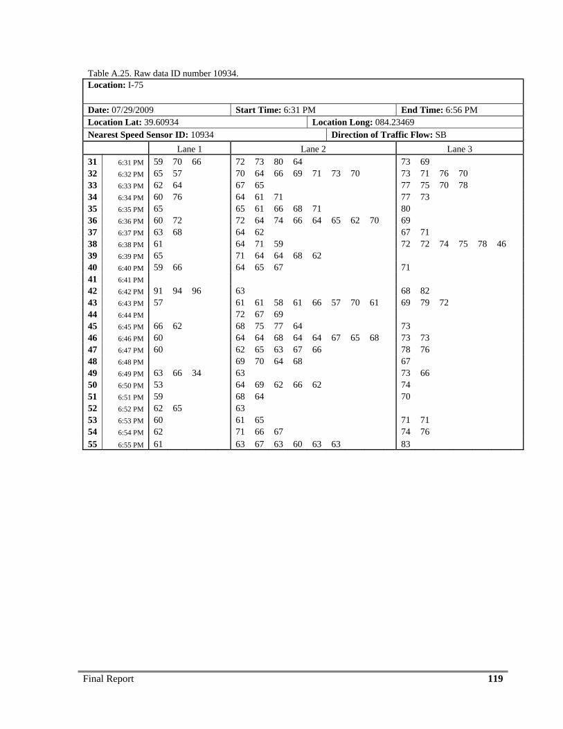
Final Report 119


Date: 07/29/2009 Start Time: 6:31 PM End Time: 6:56 PM Location Lat: 39.60934 Location Long: 084.23469 Nearest Speed Sensor ID: 10934 Direction of Traffic Flow: SB Lane 1 Lane 2 Lane 3 31 6:31 PM 59 70 66 72 73 80 64 73 69 32 6:32 PM 65 57 70 64 66 69 71 73 70 73 71 76 70 33 6:33 PM 62 64 67 65 77 75 70 78 34 6:34 PM 60 76 64 61 71 77 73 35 6:35 PM 65 65 61 66 68 71 80 36 6:36 PM 60 72 72 64 74 66 64 65 62 70 69 37 6:37 PM 63 68 64 62 67 71 38 6:38 PM 61 64 71 59 72 72 74 75 78 46 39 6:39 PM 65 71 64 64 68 62 40 6:40 PM 59 66 64 65 67 71 41 6:41 PM 42 6:42 PM 91 94 96 63 68 82 43 6:43 PM 57 61 61 58 61 66 57 70 61 69 79 72 44 6:44 PM 72 67 69 45 6:45 PM 66 62 68 75 77 64 73 46 6:46 PM 60 64 64 68 64 64 67 65 68 73 73 47 6:47 PM 60 62 65 63 67 66 78 76 48 6:48 PM 69 70 64 68 67 49 6:49 PM 63 66 34 63 73 66 50 6:50 PM 53 64 69 62 66 62 74 51 6:51 PM 59 68 64 70 52 6:52 PM 62 65 63 53 6:53 PM 60 61 65 71 71 54 6:54 PM 62 71 66 67 74 76 55 6:55 PM 61 63 67 63 60 63 63 83

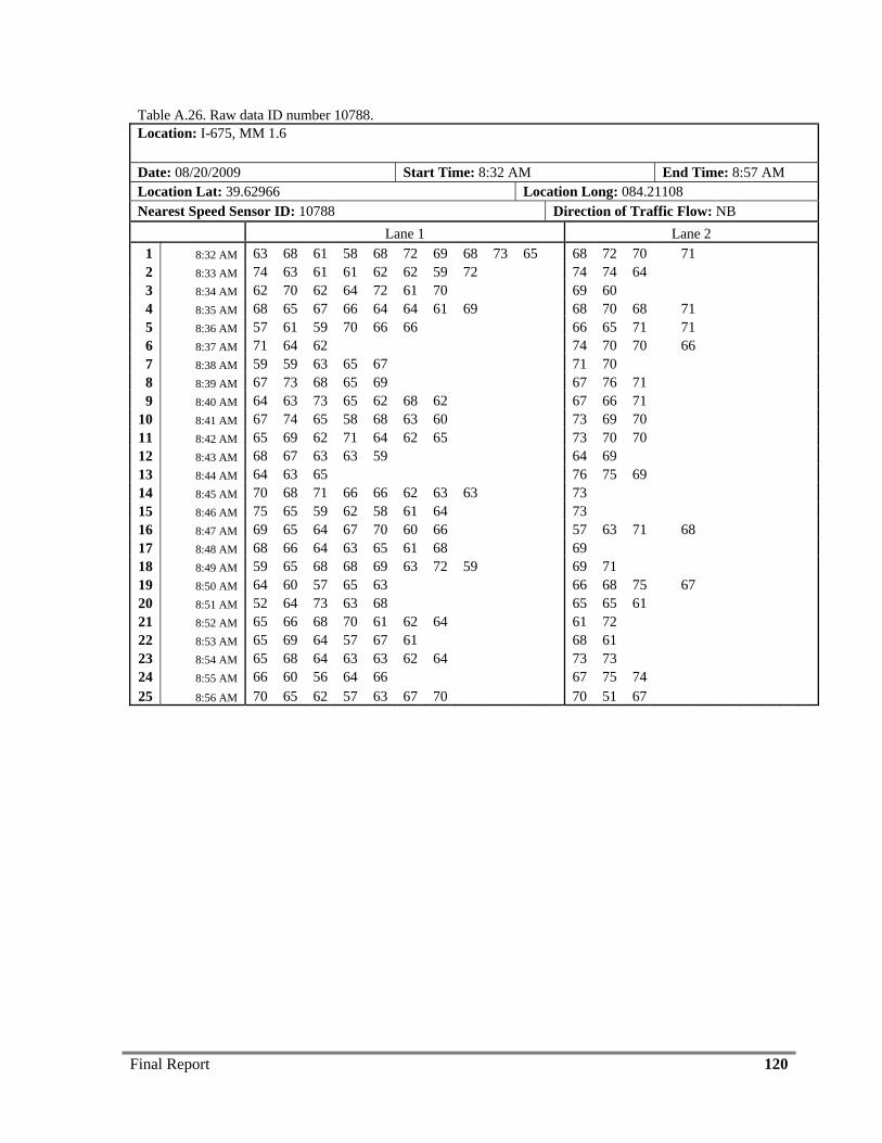
Final Report 120

Table A.26. Raw data ID number 10788. Location: I-675, MM 1.6

Date: 08/20/2009 Start Time: 8:32 AM End Time: 8:57 AM Location Lat: 39.62966 Location Long: 084.21108 Nearest Speed Sensor ID: 10788 Direction of Traffic Flow: NB Lane 1 Lane 2

1 8:32 AM 63 68 61 58 68 72 69 68 73 65 68 72 70 71 2 8:33 AM 74 63 61 61 62 62 59 72 74 74 64 3 8:34 AM 62 70 62 64 72 61 70 69 60 4 8:35 AM 68 65 67 66 64 64 61 69 68 70 68 71 5 8:36 AM 57 61 59 70 66 66 66 65 71 71 6 8:37 AM 71 64 62 74 70 70 66 7 8:38 AM 59 59 63 65 67 71 70 8 8:39 AM 67 73 68 65 69 67 76 71 9 8:40 AM 64 63 73 65 62 68 62 67 66 71

10 8:41 AM 67 74 65 58 68 63 60 73 69 70 11 8:42 AM 65 69 62 71 64 62 65 73 70 70 12 8:43 AM 68 67 63 63 59 64 69 13 8:44 AM 64 63 65 76 75 69 14 8:45 AM 70 68 71 66 66 62 63 63 73 15 8:46 AM 75 65 59 62 58 61 64 73 16 8:47 AM 69 65 64 67 70 60 66 57 63 71 68 17 8:48 AM 68 66 64 63 65 61 68 69 18 8:49 AM 59 65 68 68 69 63 72 59 69 71 19 8:50 AM 64 60 57 65 63 66 68 75 67 20 8:51 AM 52 64 73 63 68 65 65 61 21 8:52 AM 65 66 68 70 61 62 64 61 72 22 8:53 AM 65 69 64 57 67 61 68 61 23 8:54 AM 65 68 64 63 63 62 64 73 73 24 8:55 AM 66 60 56 64 66 67 75 74 25 8:56 AM 70 65 62 57 63 67 70 70 51 67

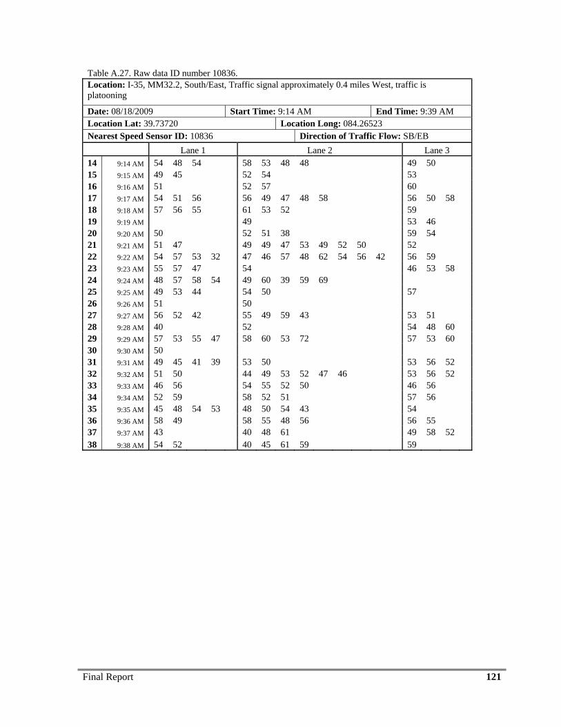
Final Report 121

Table A.27. Raw data ID number 10836. Location: I-35, MM32.2, South/East, Traffic signal approximately 0.4 miles West, traffic is platooning

Date: 08/18/2009 Start Time: 9:14 AM End Time: 9:39 AM Location Lat: 39.73720 Location Long: 084.26523 Nearest Speed Sensor ID: 10836 Direction of Traffic Flow: SB/EB Lane 1 Lane 2 Lane 3 14 9:14 AM 54 48 54 58 53 48 48 49 50 15 9:15 AM 49 45 52 54 53 16 9:16 AM 51 52 57 60 17 9:17 AM 54 51 56 56 49 47 48 58 56 50 58 18 9:18 AM 57 56 55 61 53 52 59 19 9:19 AM 49 53 46 20 9:20 AM 50 52 51 38 59 54 21 9:21 AM 51 47 49 49 47 53 49 52 50 52 22 9:22 AM 54 57 53 32 47 46 57 48 62 54 56 42 56 59 23 9:23 AM 55 57 47 54 46 53 58 24 9:24 AM 48 57 58 54 49 60 39 59 69 25 9:25 AM 49 53 44 54 50 57 26 9:26 AM 51 50 27 9:27 AM 56 52 42 55 49 59 43 53 51 28 9:28 AM 40 52 54 48 60 29 9:29 AM 57 53 55 47 58 60 53 72 57 53 60 30 9:30 AM 50 31 9:31 AM 49 45 41 39 53 50 53 56 52 32 9:32 AM 51 50 44 49 53 52 47 46 53 56 52 33 9:33 AM 46 56 54 55 52 50 46 56 34 9:34 AM 52 59 58 52 51 57 56 35 9:35 AM 45 48 54 53 48 50 54 43 54 36 9:36 AM 58 49 58 55 48 56 56 55 37 9:37 AM 43 40 48 61 49 58 52 38 9:38 AM 54 52 40 45 61 59 59

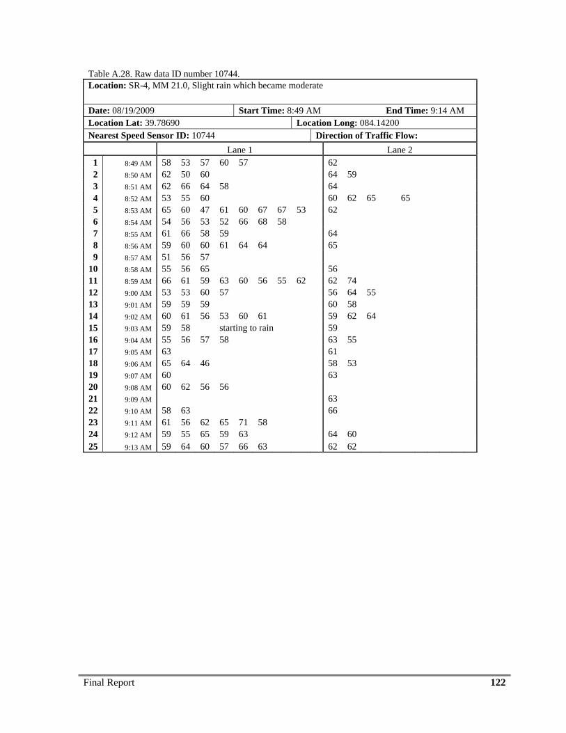
Final Report 122

Table A.28. Raw data ID number 10744. Location: SR-4, MM 21.0, Slight rain which became moderate

Date: 08/19/2009 Start Time: 8:49 AM End Time: 9:14 AM Location Lat: 39.78690 Location Long: 084.14200 Nearest Speed Sensor ID: 10744 Direction of Traffic Flow: Lane 1 Lane 2

1 8:49 AM 58 53 57 60 57 62 2 8:50 AM 62 50 60 64 59 3 8:51 AM 62 66 64 58 64 4 8:52 AM 53 55 60 60 62 65 65 5 8:53 AM 65 60 47 61 60 67 67 53 62 6 8:54 AM 54 56 53 52 66 68 58 7 8:55 AM 61 66 58 59 64 8 8:56 AM 59 60 60 61 64 64 65 9 8:57 AM 51 56 57

10 8:58 AM 55 56 65 56 11 8:59 AM 66 61 59 63 60 56 55 62 62 74 12 9:00 AM 53 53 60 57 56 64 55 13 9:01 AM 59 59 59 60 58 14 9:02 AM 60 61 56 53 60 61 59 62 64 15 9:03 AM 59 58 starting to rain 59 16 9:04 AM 55 56 57 58 63 55 17 9:05 AM 63 61 18 9:06 AM 65 64 46 58 53 19 9:07 AM 60 63 20 9:08 AM 60 62 56 56 21 9:09 AM 63 22 9:10 AM 58 63 66 23 9:11 AM 61 56 62 65 71 58 24 9:12 AM 59 55 65 59 63 64 60 25 9:13 AM 59 64 60 57 66 63 62 62

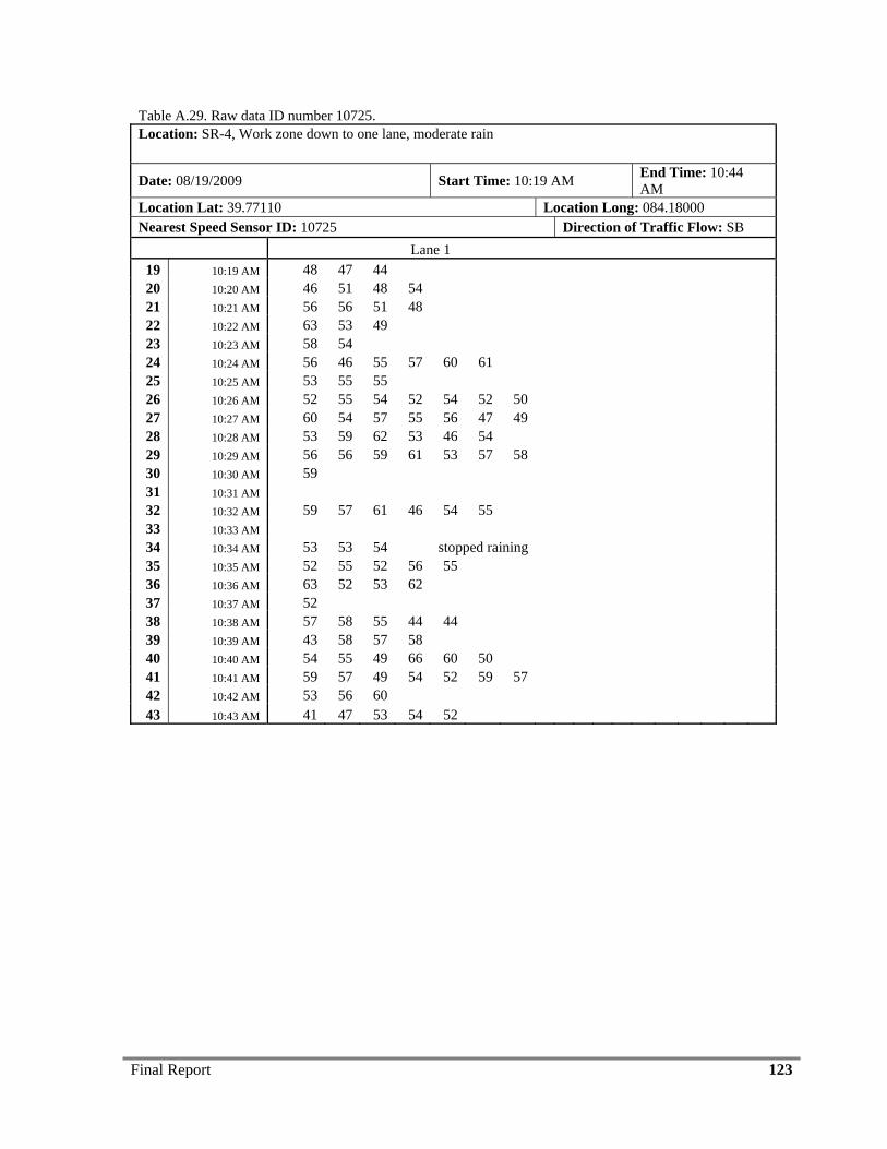
Final Report 123

Table A.29. Raw data ID number 10725. Location: SR-4, Work zone down to one lane, moderate rain

Date: 08/19/2009 Start Time: 10:19 AM End Time: 10:44 AM

Location Lat: 39.77110 Location Long: 084.18000 Nearest Speed Sensor ID: 10725 Direction of Traffic Flow: SB Lane 1

19 10:19 AM 48 47 44 20 10:20 AM 46 51 48 54 21 10:21 AM 56 56 51 48 22 10:22 AM 63 53 49 23 10:23 AM 58 54 24 10:24 AM 56 46 55 57 60 61 25 10:25 AM 53 55 55 26 10:26 AM 52 55 54 52 54 52 50 27 10:27 AM 60 54 57 55 56 47 49 28 10:28 AM 53 59 62 53 46 54 29 10:29 AM 56 56 59 61 53 57 58 30 10:30 AM 59 31 10:31 AM 32 10:32 AM 59 57 61 46 54 55 33 10:33 AM 34 10:34 AM 53 53 54 stopped raining 35 10:35 AM 52 55 52 56 55 36 10:36 AM 63 52 53 62 37 10:37 AM 52 38 10:38 AM 57 58 55 44 44 39 10:39 AM 43 58 57 58 40 10:40 AM 54 55 49 66 60 50 41 10:41 AM 59 57 49 54 52 59 57 42 10:42 AM 53 56 60 43 10:43 AM 41 47 53 54 52

Final Report 124

APPENDIX B

HISTOGRAMS

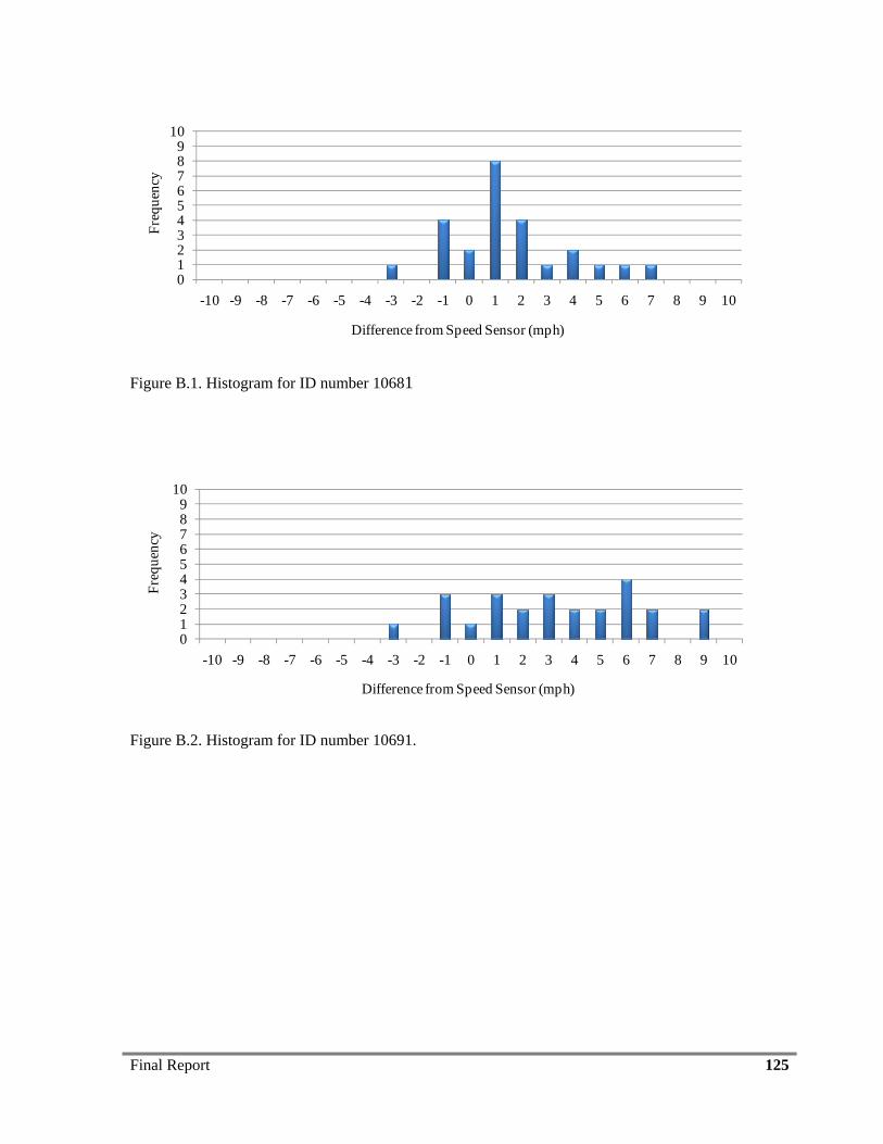
Final Report 125

0123456789

10

-10 -9 -8 -7 -6 -5 -4 -3 -2 -1 0 1 2 3 4 5 6 7 8 9 10

Freq

uenc

y


Figure B.1. Histogram for ID number 10681

0123456789

10

-10 -9 -8 -7 -6 -5 -4 -3 -2 -1 0 1 2 3 4 5 6 7 8 9 10

Freq

uenc

y


Figure B.2. Histogram for ID number 10691.

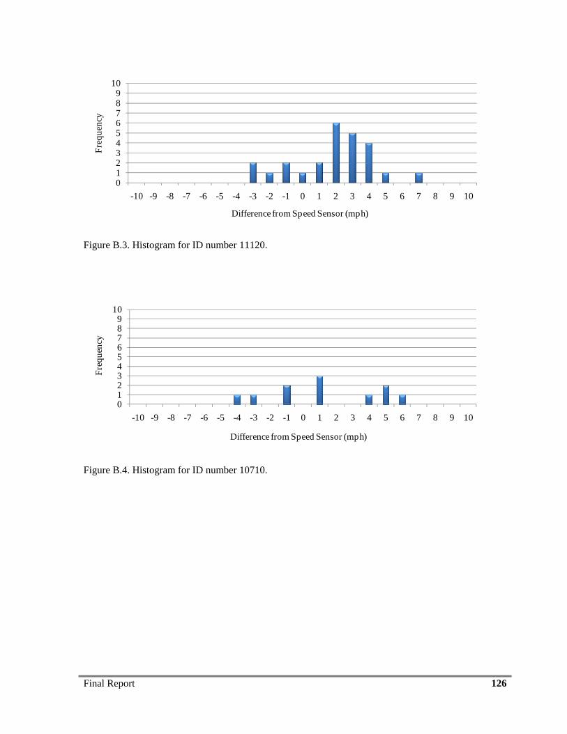
Final Report 126

0123456789

10

-10 -9 -8 -7 -6 -5 -4 -3 -2 -1 0 1 2 3 4 5 6 7 8 9 10

Freq

uenc

y



0123456789

10

-10 -9 -8 -7 -6 -5 -4 -3 -2 -1 0 1 2 3 4 5 6 7 8 9 10

Freq

uenc

y



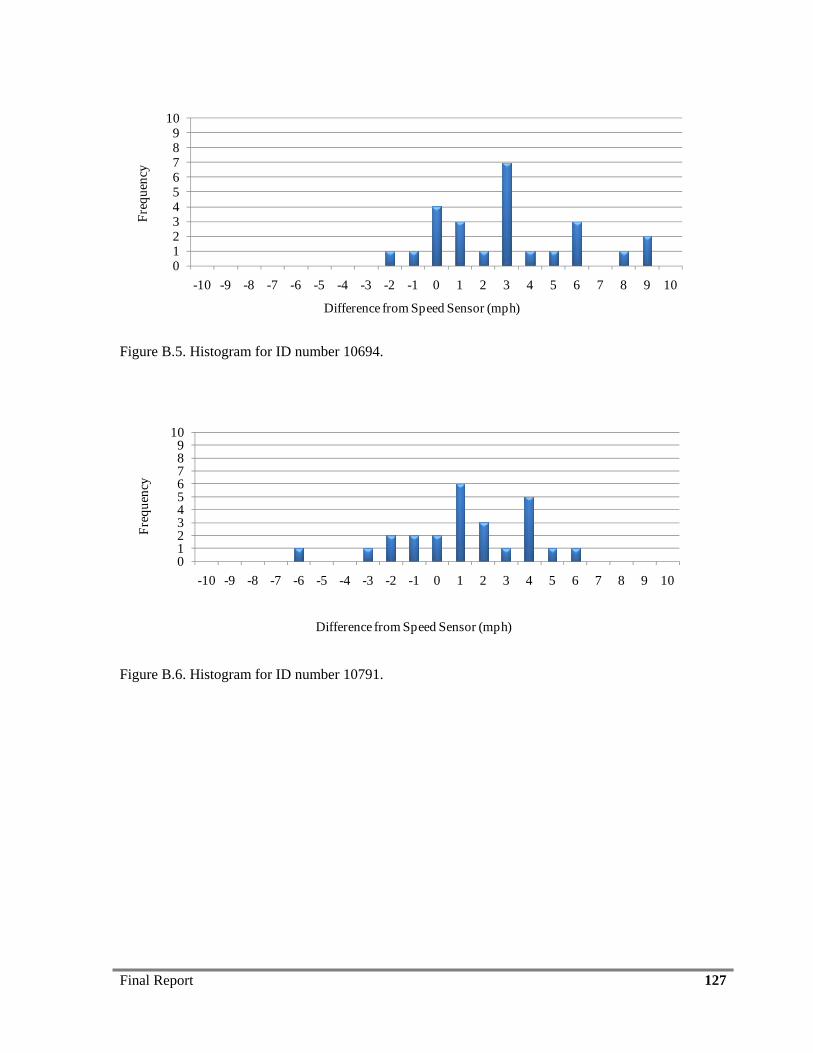
Final Report 127

0123456789

10

-10 -9 -8 -7 -6 -5 -4 -3 -2 -1 0 1 2 3 4 5 6 7 8 9 10

Freq

uenc

y



0123456789

10

-10 -9 -8 -7 -6 -5 -4 -3 -2 -1 0 1 2 3 4 5 6 7 8 9 10

Freq

uenc

y



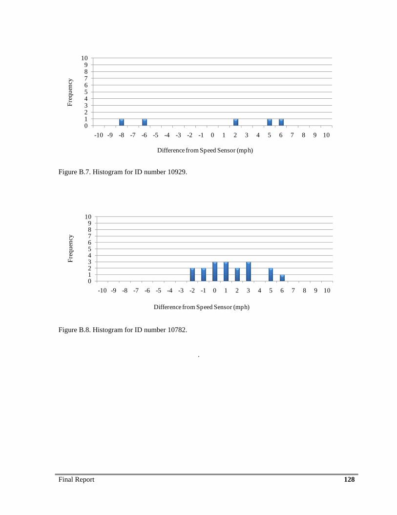
Final Report 128

0123456789

10

-10 -9 -8 -7 -6 -5 -4 -3 -2 -1 0 1 2 3 4 5 6 7 8 9 10

Freq

uenc

y



0123456789

10

-10 -9 -8 -7 -6 -5 -4 -3 -2 -1 0 1 2 3 4 5 6 7 8 9 10

Freq

uenc

y



.

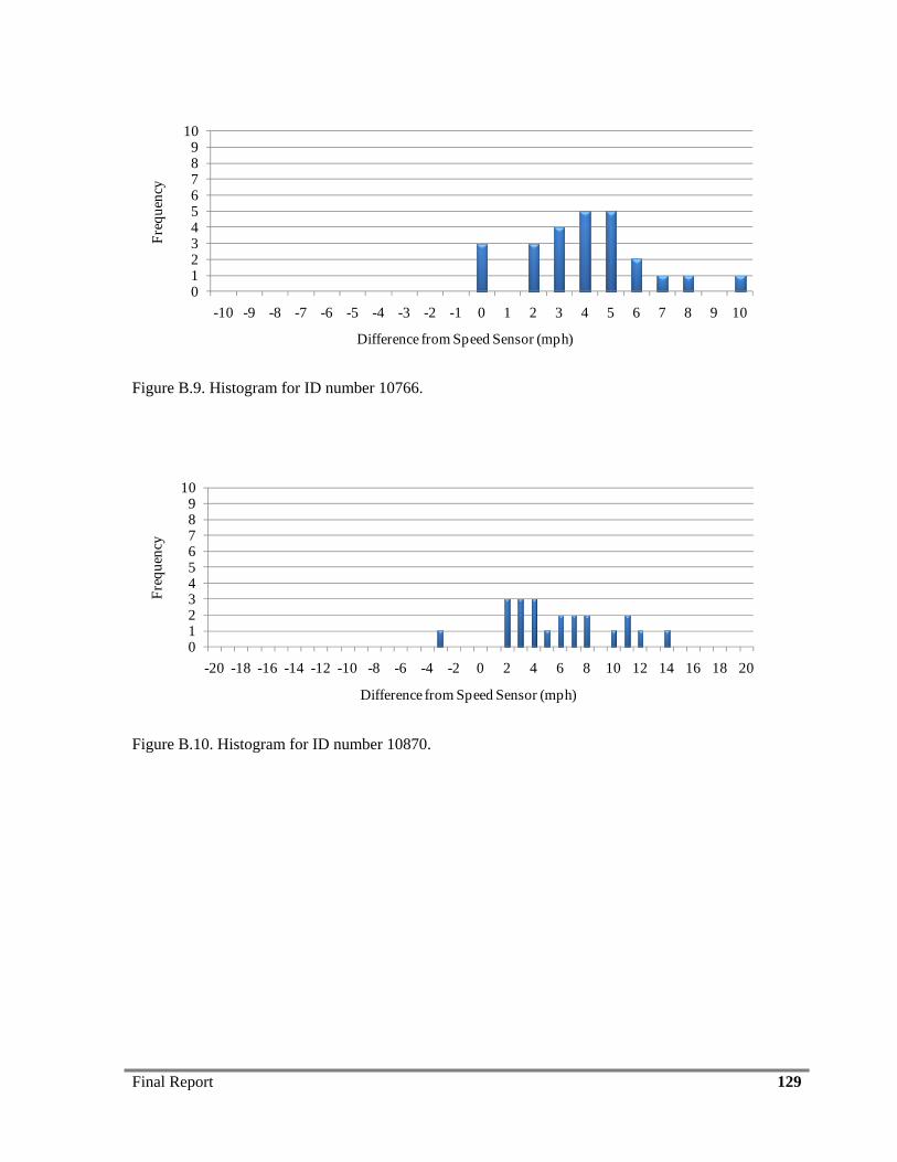
Final Report 129

0123456789

10

-10 -9 -8 -7 -6 -5 -4 -3 -2 -1 0 1 2 3 4 5 6 7 8 9 10

Freq

uenc

y



0123456789

10

-20 -18 -16 -14 -12 -10 -8 -6 -4 -2 0 2 4 6 8 10 12 14 16 18 20

Freq

uenc

y



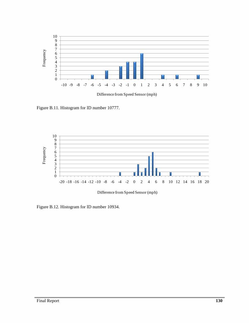
Final Report 130

0123456789

10

-10 -9 -8 -7 -6 -5 -4 -3 -2 -1 0 1 2 3 4 5 6 7 8 9 10

Freq

uenc

y



0123456789

10

-20 -18 -16 -14 -12 -10 -8 -6 -4 -2 0 2 4 6 8 10 12 14 16 18 20

Freq

uenc

y



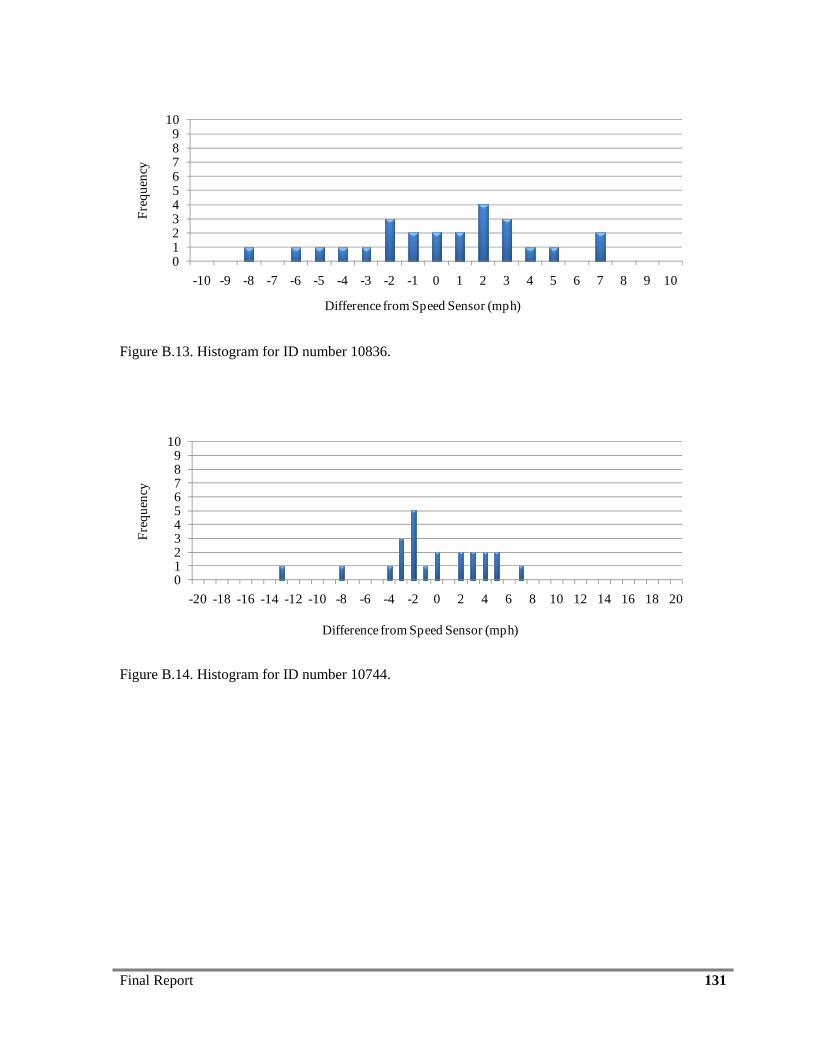
Final Report 131

0123456789

10

-10 -9 -8 -7 -6 -5 -4 -3 -2 -1 0 1 2 3 4 5 6 7 8 9 10

Freq

uenc

y



0123456789

10

-20 -18 -16 -14 -12 -10 -8 -6 -4 -2 0 2 4 6 8 10 12 14 16 18 20

Freq

uenc

y



Final Report 132

APPENDIX C

BLUETOOTH AND FLOATING CAR COMPARISON

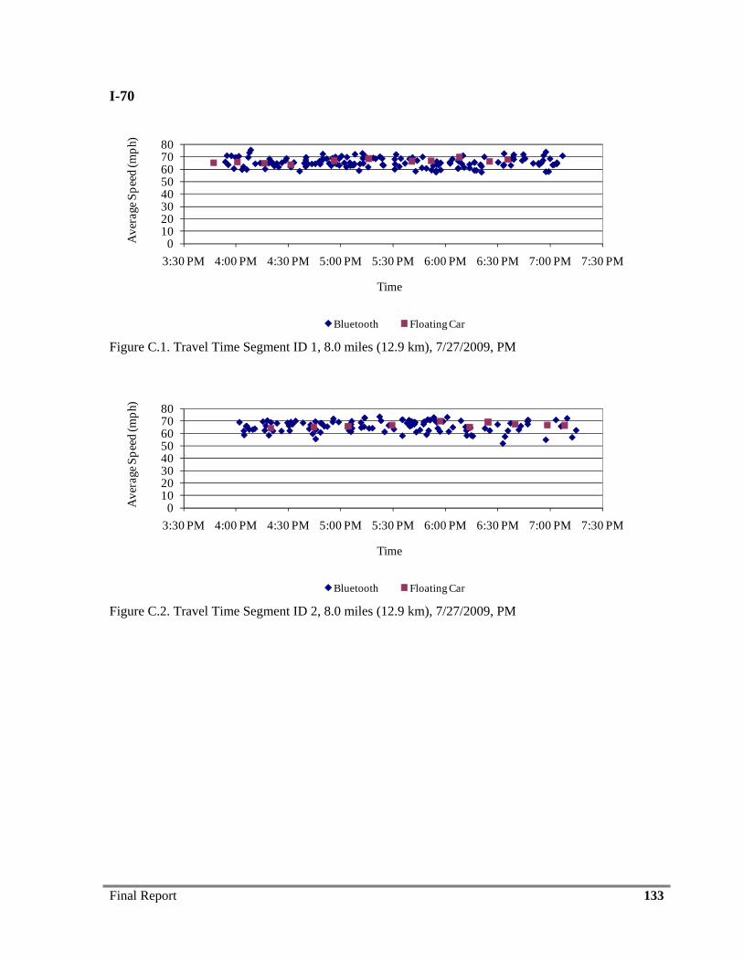
Final Report 133

I-70

01020304050607080


Ave

rage

Spe

ed (m

ph).

Time


Figure C.1. Travel Time Segment ID 1, 8.0 miles (12.9 km), 7/27/2009, PM

01020304050607080


Ave

rage

Spe

ed (m

ph).

Time



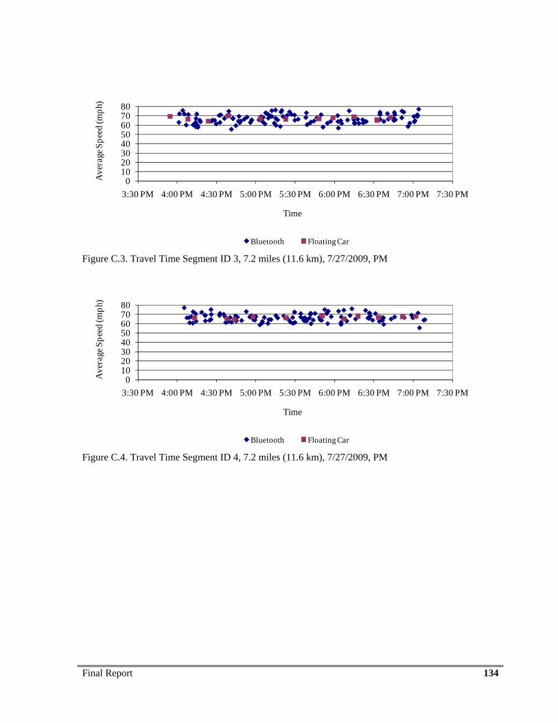
Final Report 134

01020304050607080


Ave

rage

Spe

ed (m

ph).

Time



01020304050607080


Ave

rage

Spe

ed (m

ph).

Time



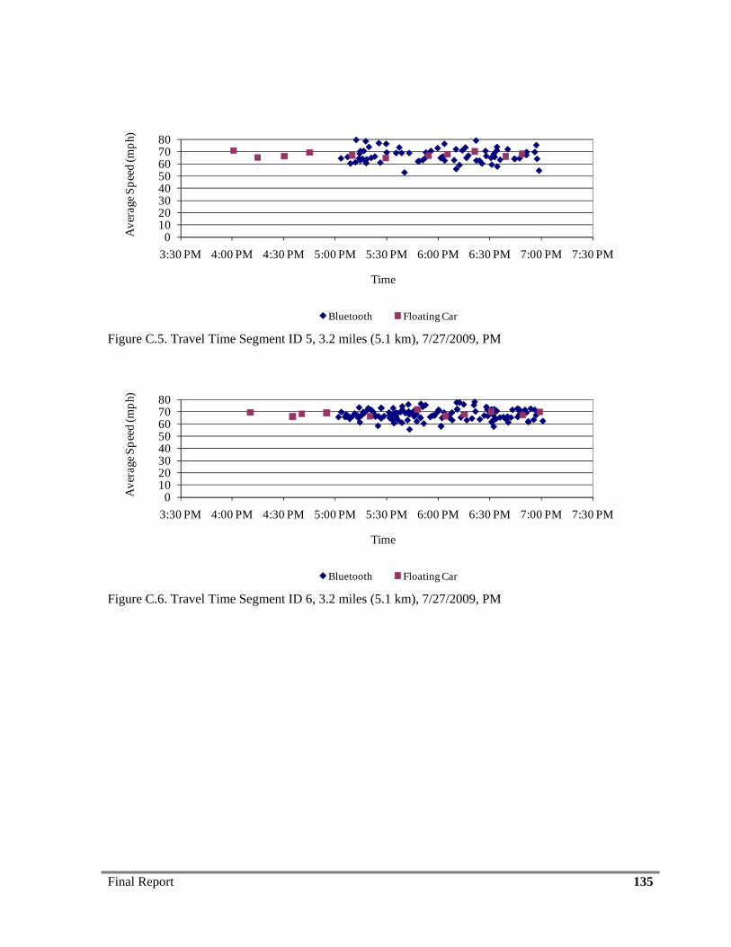
Final Report 135

01020304050607080


Ave

rage

Spe

ed (m

ph).

Time



01020304050607080


Ave

rage

Spe

ed (m

ph).

Time



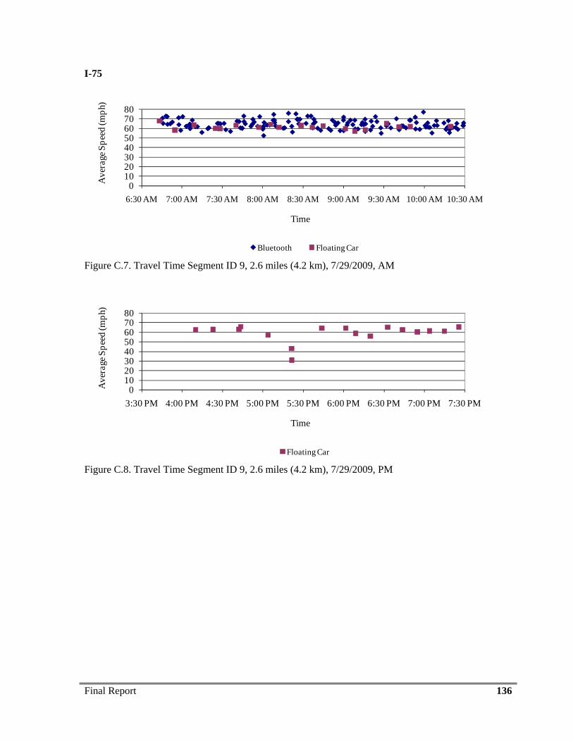
Final Report 136

I-75

01020304050607080


Ave

rage

Spe

ed (m

ph).

Time


Figure C.7. Travel Time Segment ID 9, 2.6 miles (4.2 km), 7/29/2009, AM

01020304050607080


Ave

rage

Spe

ed (m

ph).

Time

Floating Car


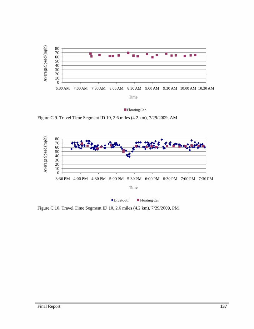
Final Report 137

01020304050607080


Ave

rage

Spe

ed (m

ph).

Time

Floating Car


01020304050607080


Ave

rage

Spe

ed (m

ph).

Time



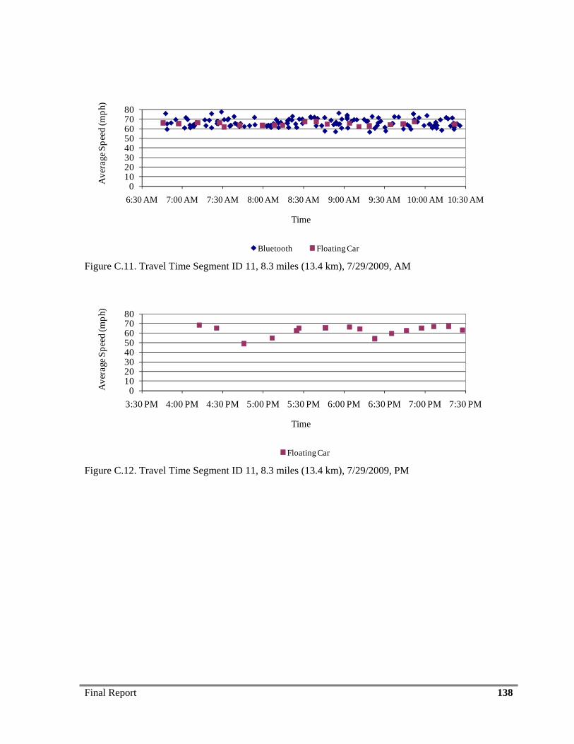
Final Report 138

01020304050607080


Ave

rage

Spe

ed (m

ph).

Time



01020304050607080


Ave

rage

Spe

ed (m

ph).

Time

Floating Car


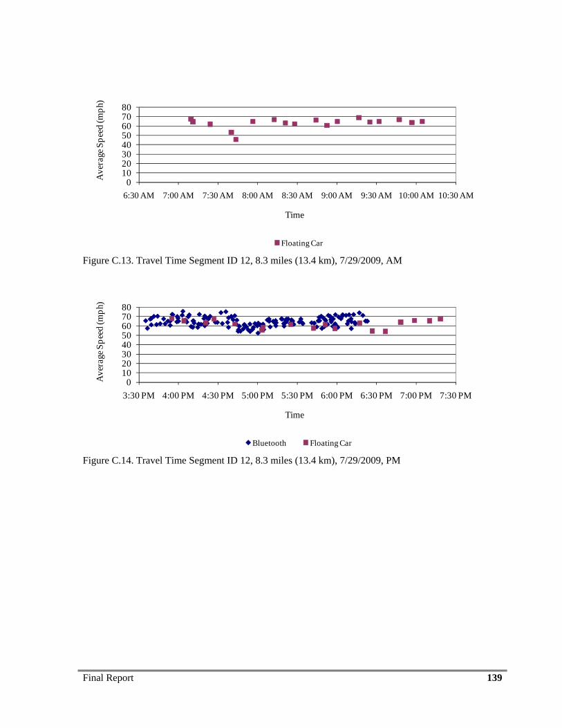
Final Report 139

01020304050607080


Ave

rage

Spe

ed (m

ph).

Time

Floating Car


01020304050607080


Ave

rage

Spe

ed (m

ph).

Time



Final Report 140

01020304050607080


Ave

rage

Spe

ed (m

ph).

Time

Floating Car


01020304050607080


Ave

rage

Spe

ed (m

ph).

Time

Floating Car


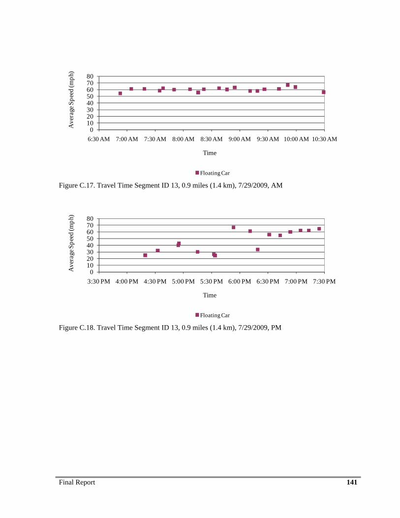
Final Report 141

01020304050607080


Ave

rage

Spe

ed (m

ph).

Time

Floating Car


01020304050607080


Ave

rage

Spe

ed (m

ph).

Time

Floating Car


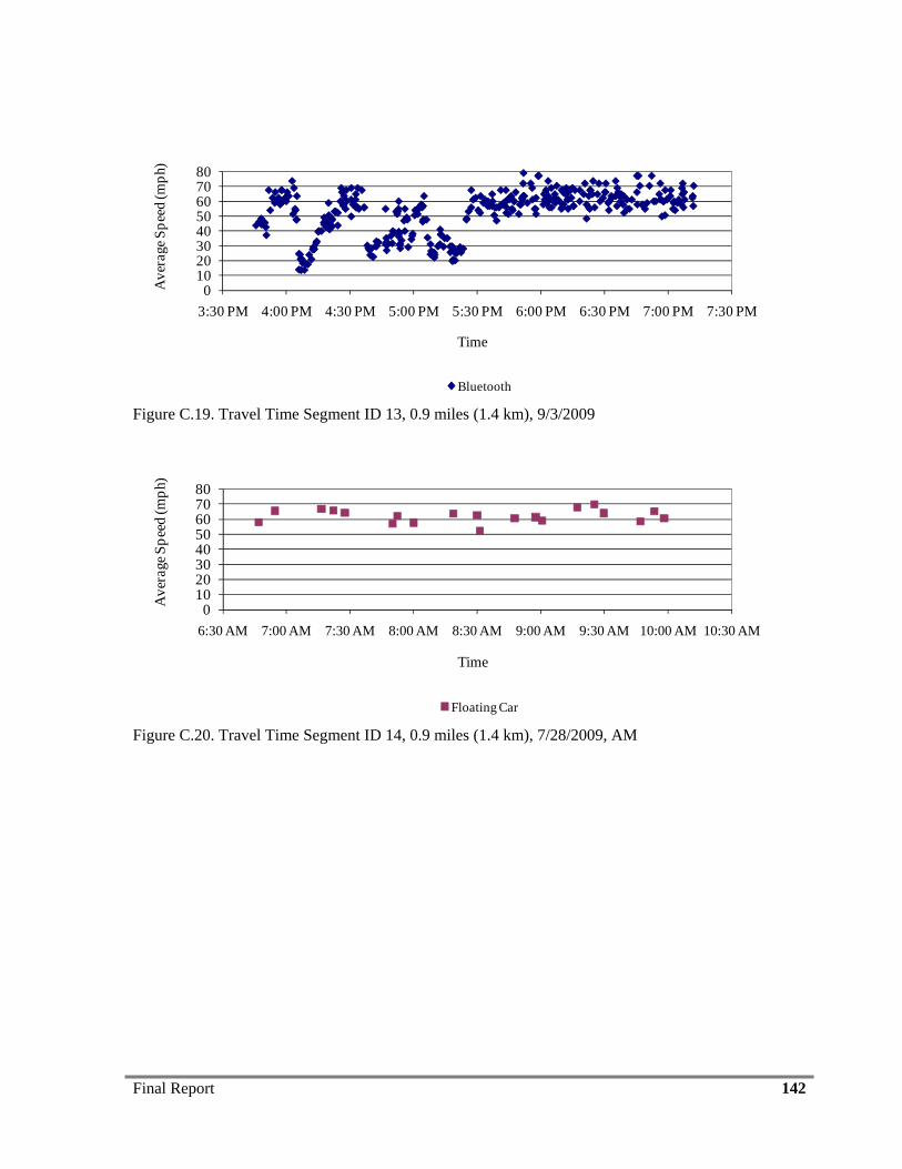
Final Report 142

01020304050607080


Ave

rage

Spe

ed (m

ph).

Time

Bluetooth

Figure C.19. Travel Time Segment ID 13, 0.9 miles (1.4 km), 9/3/2009

01020304050607080


Ave

rage

Spe

ed (m

ph).

Time

Floating Car


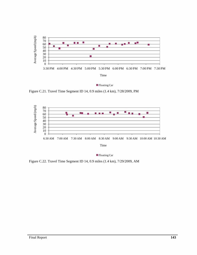
Final Report 143

01020304050607080


Ave

rage

Spe

ed (m

ph).

Time

Floating Car


01020304050607080


Ave

rage

Spe

ed (m

ph).

Time

Floating Car


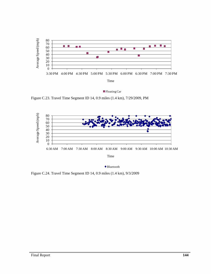
Final Report 144

01020304050607080


Ave

rage

Spe

ed (m

ph).

Time

Floating Car


01020304050607080


Ave

rage

Spe

ed (m

ph).

Time

Bluetooth


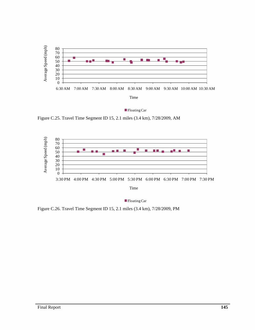
Final Report 145

01020304050607080


Ave

rage

Spe

ed (m

ph).

Time

Floating Car


01020304050607080


Ave

rage

Spe

ed (m

ph).

Time

Floating Car


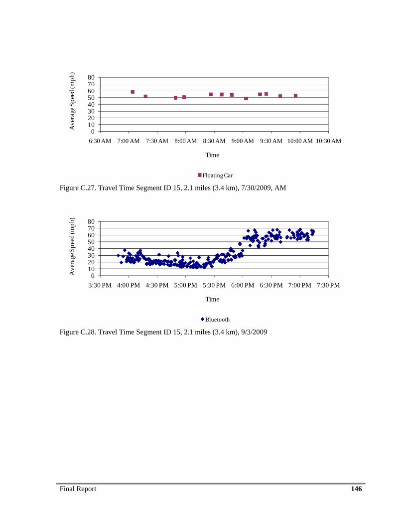
Final Report 146

01020304050607080


Ave

rage

Spe

ed (m

ph).

Time

Floating Car


01020304050607080


Ave

rage

Spe

ed (m

ph).

Time

Bluetooth


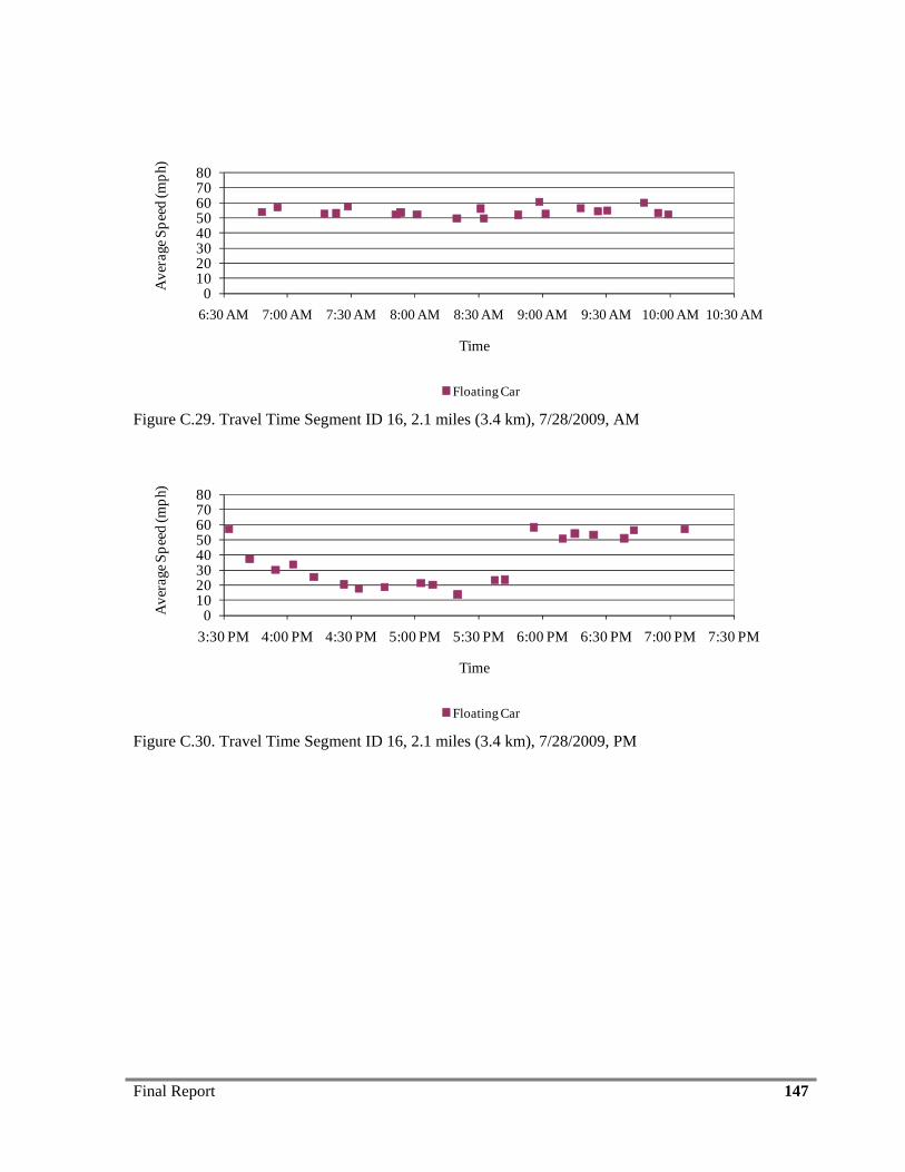
Final Report 147

01020304050607080


Ave

rage

Spe

ed (m

ph).

Time

Floating Car


01020304050607080


Ave

rage

Spe

ed (m

ph).

Time

Floating Car


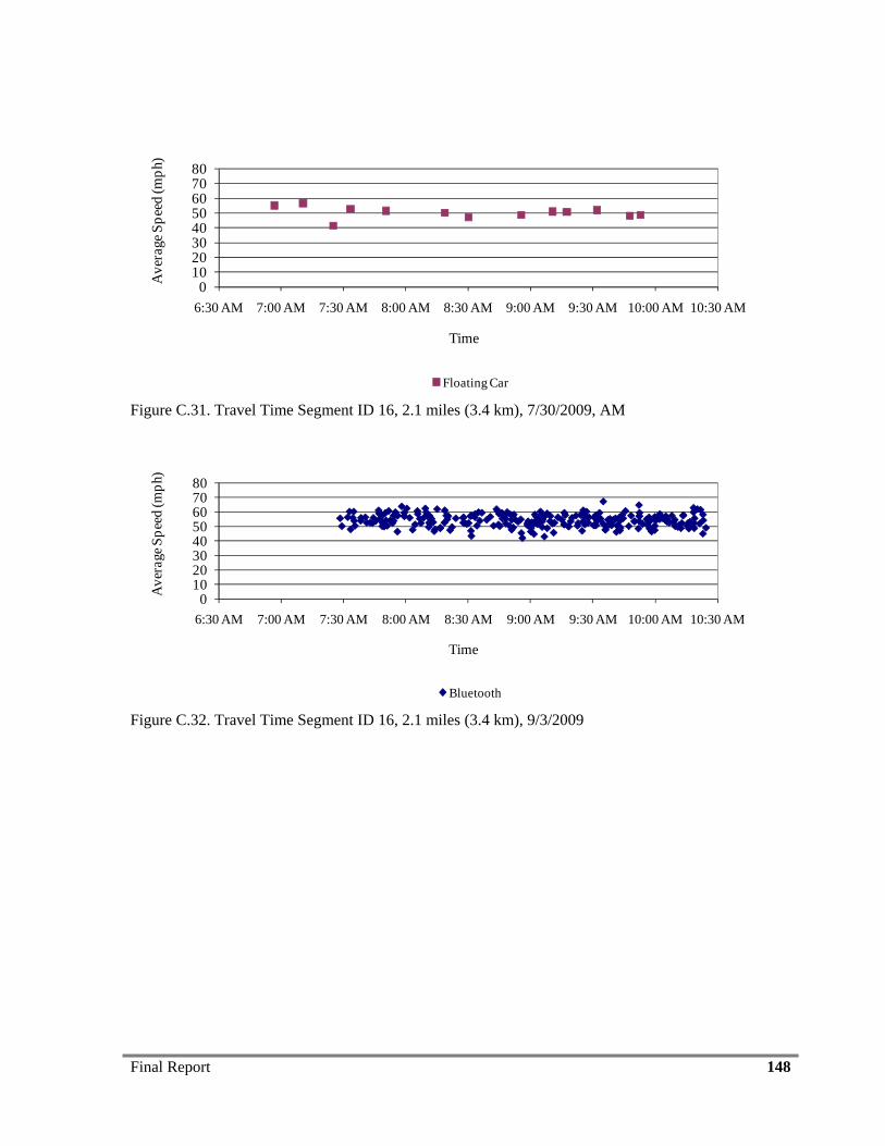
Final Report 148

01020304050607080


Ave

rage

Spe

ed (m

ph).

Time

Floating Car


01020304050607080


Ave

rage

Spe

ed (m

ph).

Time

Bluetooth


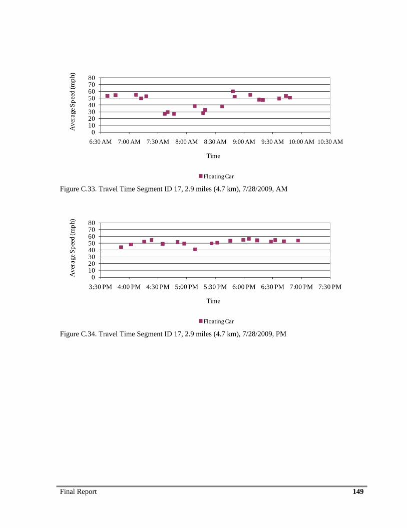
Final Report 149

01020304050607080


Ave

rage

Spe

ed (m

ph).

Time

Floating Car


01020304050607080


Ave

rage

Spe

ed (m

ph).

Time

Floating Car


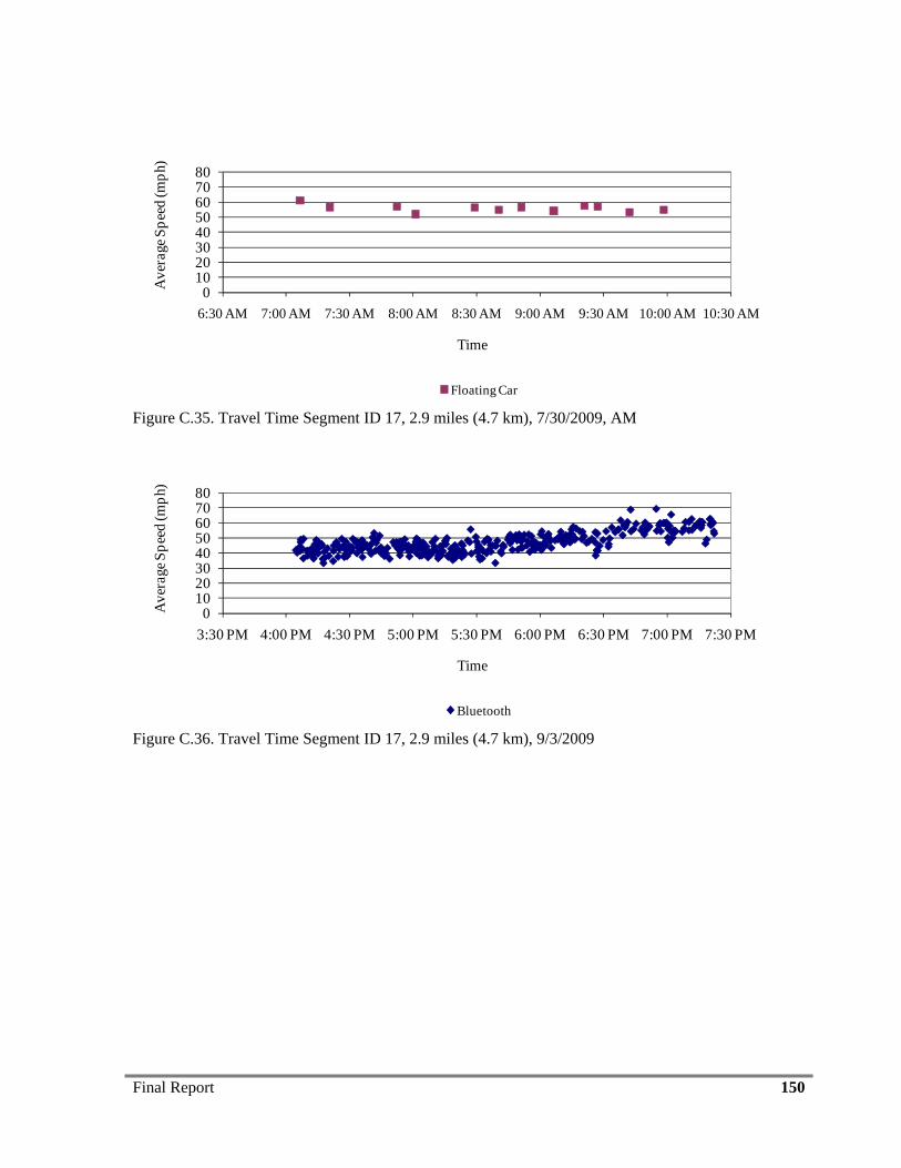
Final Report 150

01020304050607080


Ave

rage

Spe

ed (m

ph).

Time

Floating Car


01020304050607080


Ave

rage

Spe

ed (m

ph).

Time

Bluetooth


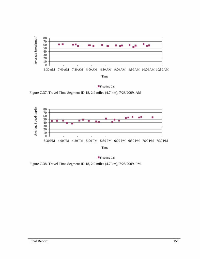
Final Report 151

01020304050607080


Ave

rage

Spe

ed (m

ph).

Time

Floating Car


01020304050607080


Ave

rage

Spe

ed (m

ph).

Time

Floating Car


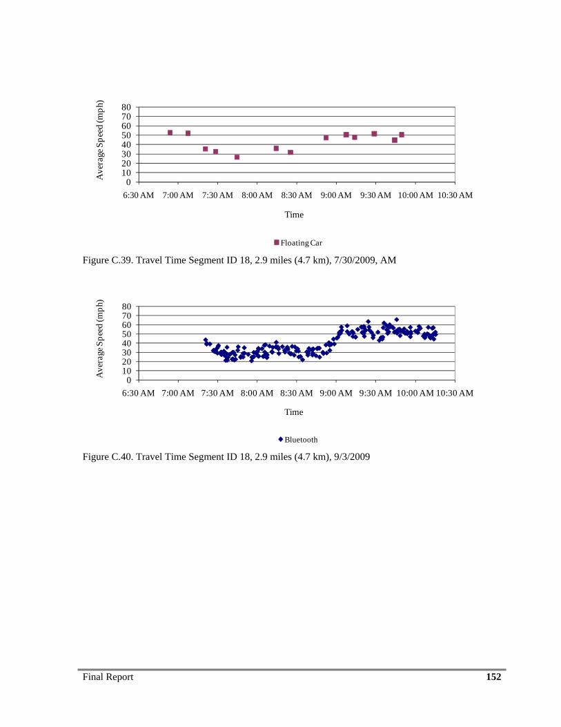
Final Report 152

01020304050607080


Ave

rage

Spe

ed (m

ph).

Time

Floating Car


01020304050607080


Ave

rage

Spe

ed (m

ph).

Time

Bluetooth


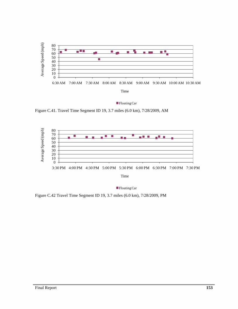
Final Report 153

01020304050607080


Ave

rage

Spe

ed (m

ph).

Time

Floating Car


01020304050607080


Ave

rage

Spe

ed (m

ph).

Time

Floating Car

Figure C.42 Travel Time Segment ID 19, 3.7 miles (6.0 km), 7/28/2009, PM

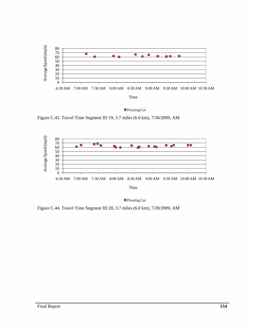
Final Report 154

01020304050607080


Ave

rage

Spe

ed (m

ph).

Time

Floating Car


01020304050607080


Ave

rage

Spe

ed (m

ph).

Time

Floating Car


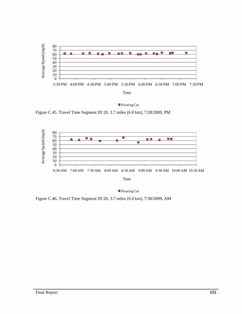
Final Report 155

01020304050607080


Ave

rage

Spe

ed (m

ph).

Time

Floating Car


01020304050607080


Ave

rage

Spe

ed (m

ph).

Time

Floating Car


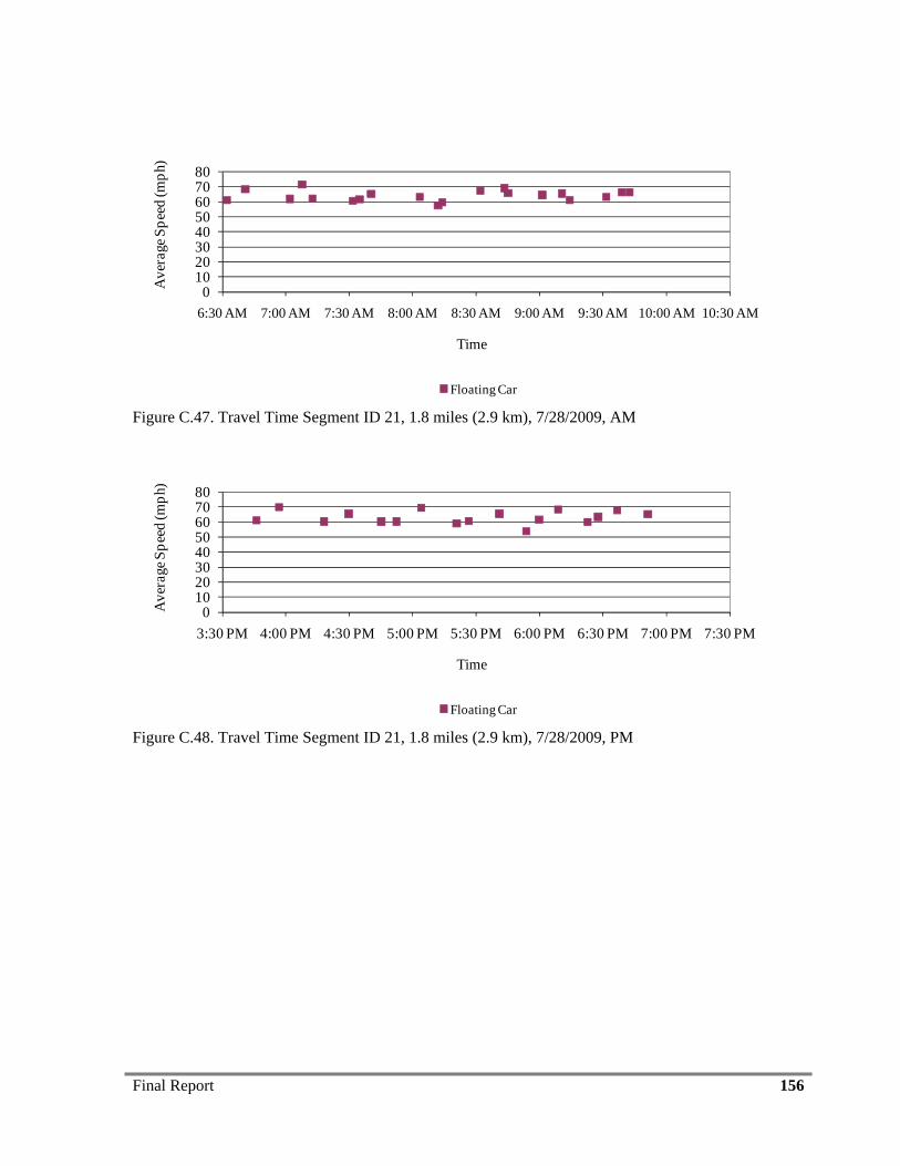
Final Report 156

01020304050607080


Ave

rage

Spe

ed (m

ph).

Time

Floating Car


01020304050607080


Ave

rage

Spe

ed (m

ph).

Time

Floating Car


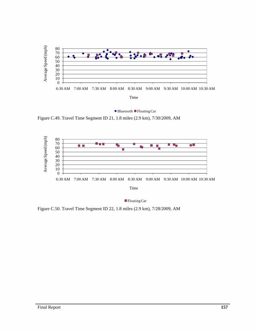
Final Report 157

01020304050607080


Ave

rage

Spe

ed (m

ph).

Time

Bluetooth Floating Car Figure C.49. Travel Time Segment ID 21, 1.8 miles (2.9 km), 7/30/2009, AM

01020304050607080


Ave

rage

Spe

ed (m

ph).

Time

Floating Car


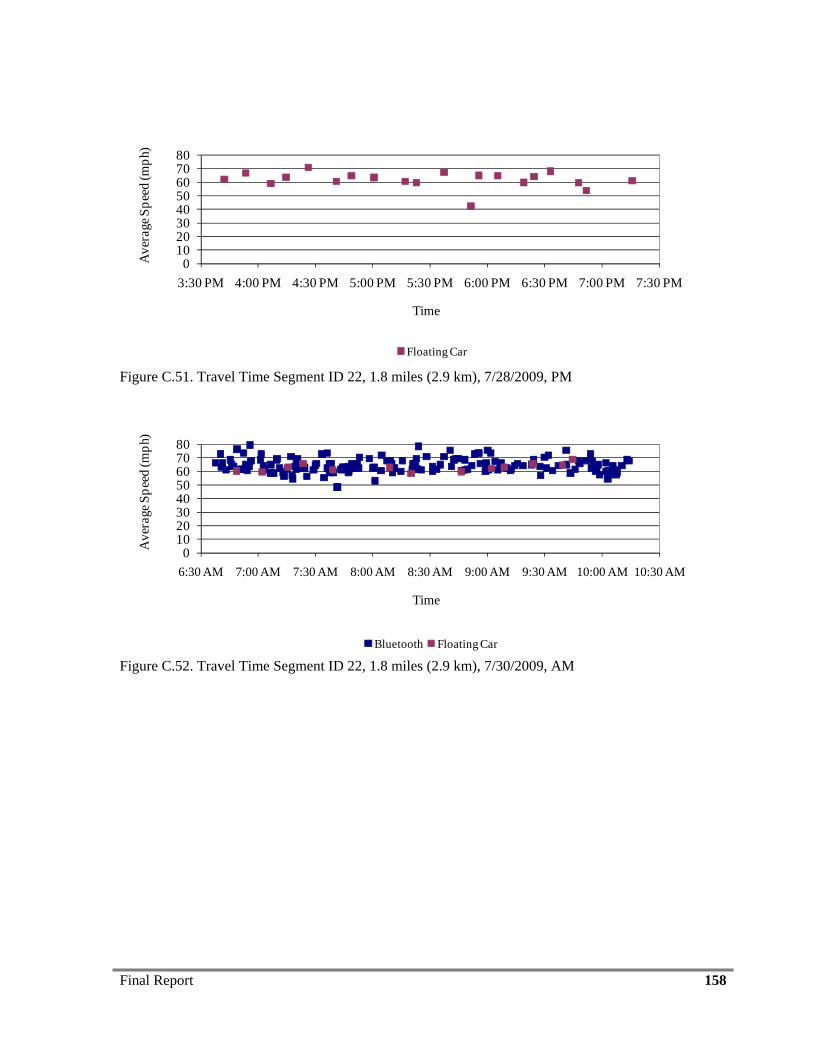
Final Report 158

01020304050607080


Ave

rage

Spe

ed (m

ph).

Time

Floating Car


01020304050607080


Ave

rage

Spe

ed (m

ph).

Time

Bluetooth Floating Car Figure C.52. Travel Time Segment ID 22, 1.8 miles (2.9 km), 7/30/2009, AM

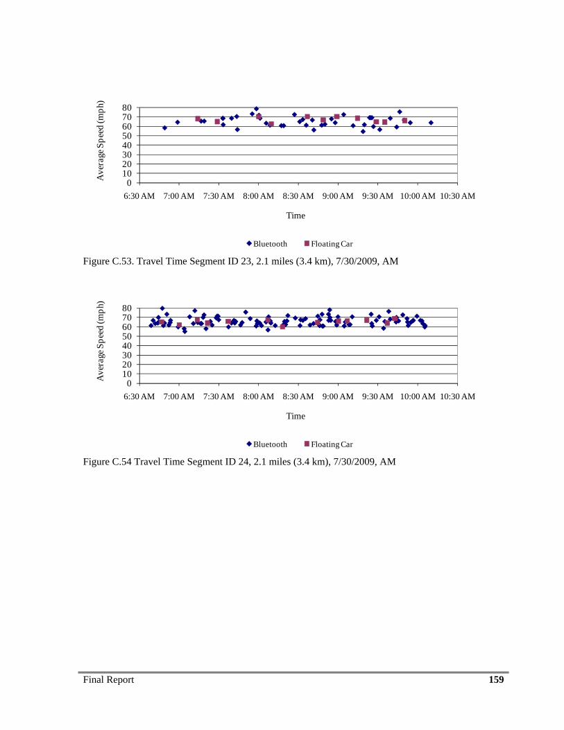
Final Report 159

01020304050607080


Ave

rage

Spe

ed (m

ph).

Time



01020304050607080


Ave

rage

Spe

ed (m

ph).

Time


Figure C.54 Travel Time Segment ID 24, 2.1 miles (3.4 km), 7/30/2009, AM

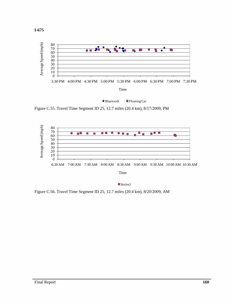
Final Report 160

I-675

01020304050607080


Ave

rage

Spe

ed (m

ph).

Time



01020304050607080


Ave

rage

Spe

ed (m

ph).

Time

Series1


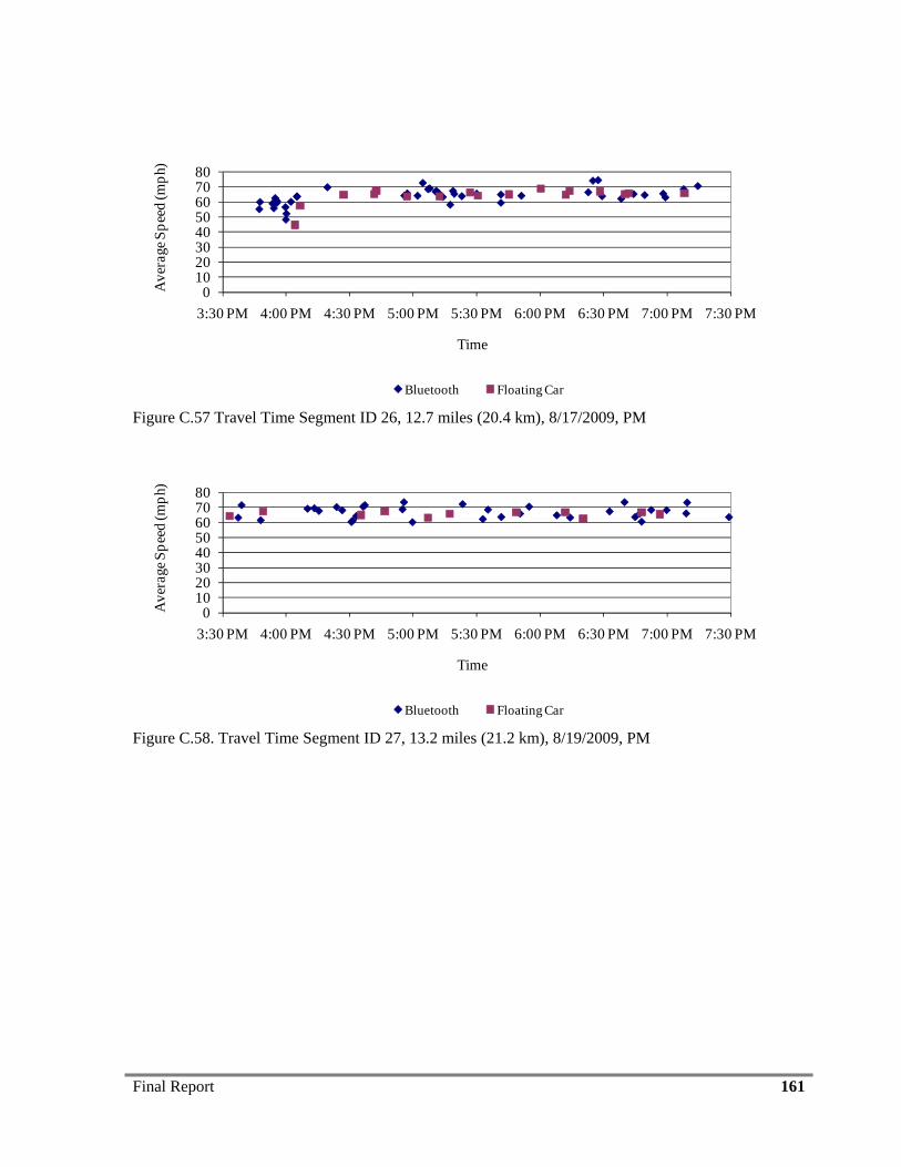
Final Report 161

01020304050607080


Ave

rage

Spe

ed (m

ph).

Time


Figure C.57 Travel Time Segment ID 26, 12.7 miles (20.4 km), 8/17/2009, PM

01020304050607080


Ave

rage

Spe

ed (m

ph).

Time



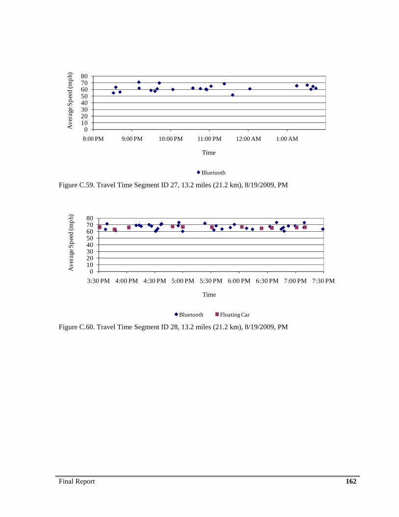
Final Report 162

01020304050607080

8:00 PM 9:00 PM 10:00 PM 11:00 PM 12:00 AM 1:00 AM

Ave

rage

Spe

ed (m

ph).

Time

Bluetooth


01020304050607080


Ave

rage

Spe

ed (m

ph).

Time



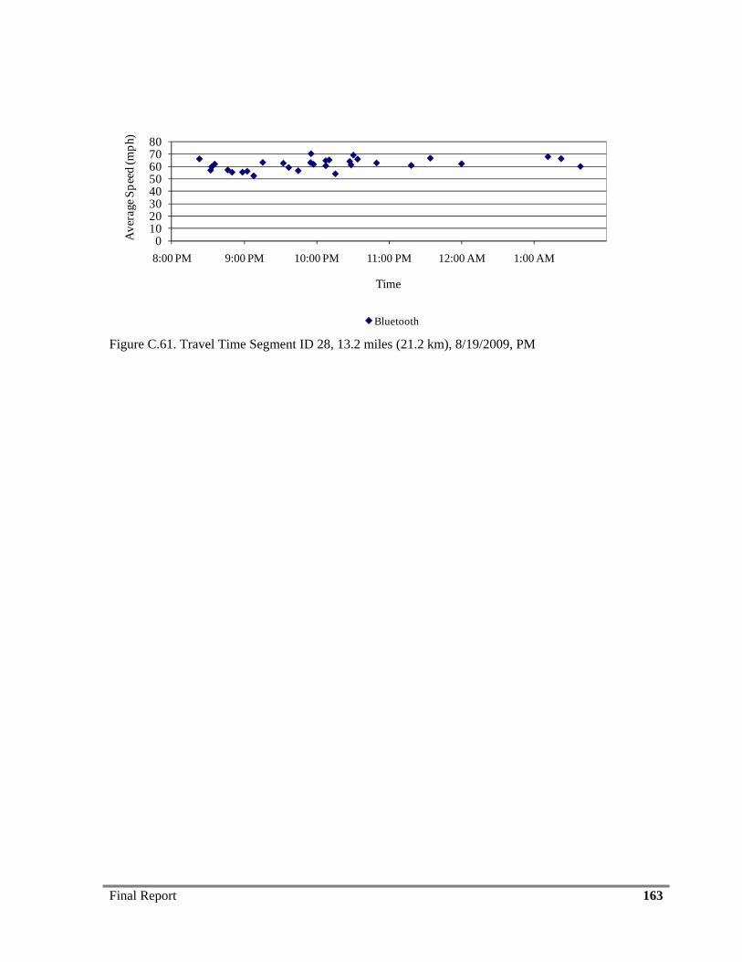
Final Report 163

01020304050607080

8:00 PM 9:00 PM 10:00 PM 11:00 PM 12:00 AM 1:00 AM

Ave

rage

Spe

ed (m

ph).

Time

Bluetooth


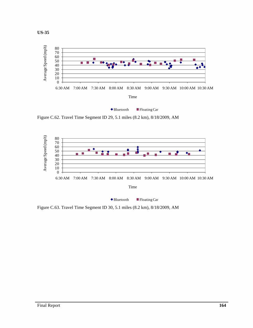
Final Report 164

US-35

01020304050607080


Ave

rage

Spe

ed (m

ph).

Time



01020304050607080


Ave

rage

Spe

ed (m

ph).

Time



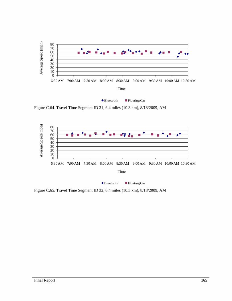
Final Report 165

01020304050607080


Ave

rage

Spe

ed (m

ph).

Time



01020304050607080


Ave

rage

Spe

ed (m

ph).

Time



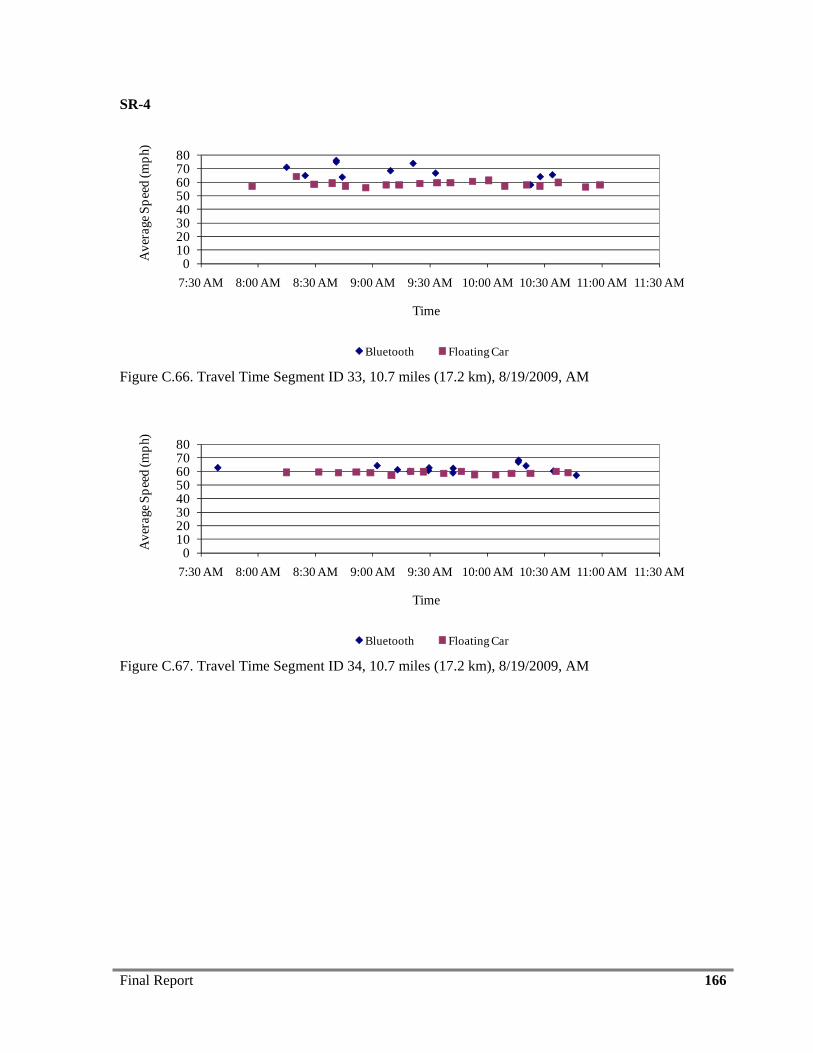
Final Report 166

SR-4

01020304050607080


Ave

rage

Spe

ed (m

ph).

Time



01020304050607080


Ave

rage

Spe

ed (m

ph).

Time



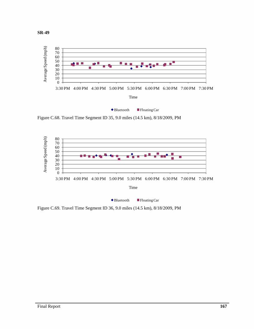
Final Report 167

SR-49

01020304050607080


Ave

rage

Spe

ed (m

ph).

Time



01020304050607080


Ave

rage

Spe

ed (m

ph).

Time



Final Report 168

APPENDIX D

STATISTICAL EVALUATION OF ODOT TRAVEL TIMES AND REFERENCE DATA

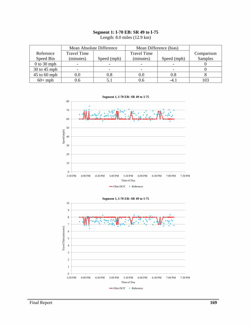
Final Report 169

Segment 1: I-70 EB: SR 49 to I-75 Length: 8.0 miles (12.9 km)

Reference Speed Bin


Samples Travel Time

(minutes) Speed (mph) Travel Time

(minutes) Speed (mph) 0 to 30 mph - - - - 0

30 to 45 mph - - - - 0 45 to 60 mph 0.0 0.8 0.0 0.8 8

60+ mph 0.6 5.1 0.6 -4.1 103

0

10

20

30

40

50

60

70

80


Spee

d (m

ph)

Time of Day

Segment 1, I-70 EB: SR 49 to I-75

Ohio DOT Reference

0

1

2

3

4

5

6

7

8

9

10


Trav

el T

ime (

min

utes

)

Time of Day

Segment 1, I-70 EB: SR 49 to I-75

Ohio DOT Reference

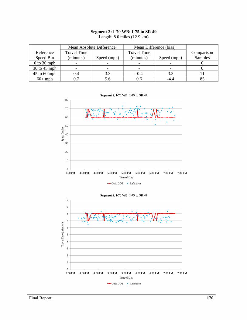
Final Report 170

Segment 2: I-70 WB: I-75 to SR 49 Length: 8.0 miles (12.9 km)

Reference Speed Bin


Samples Travel Time



30 to 45 mph - - - - 0 45 to 60 mph 0.4 3.3 -0.4 3.3 11

60+ mph 0.7 5.6 0.6 -4.4 85

0

10

20

30

40

50

60

70

80


Spee

d (m

ph)

Time of Day

Segment 2, I-70 WB: I-75 to SR 49

Ohio DOT Reference

0

1

2

3

4

5

6

7

8

9

10


Trav

el T

ime (

min

utes

)

Time of Day

Segment 2, I-70 WB: I-75 to SR 49

Ohio DOT Reference

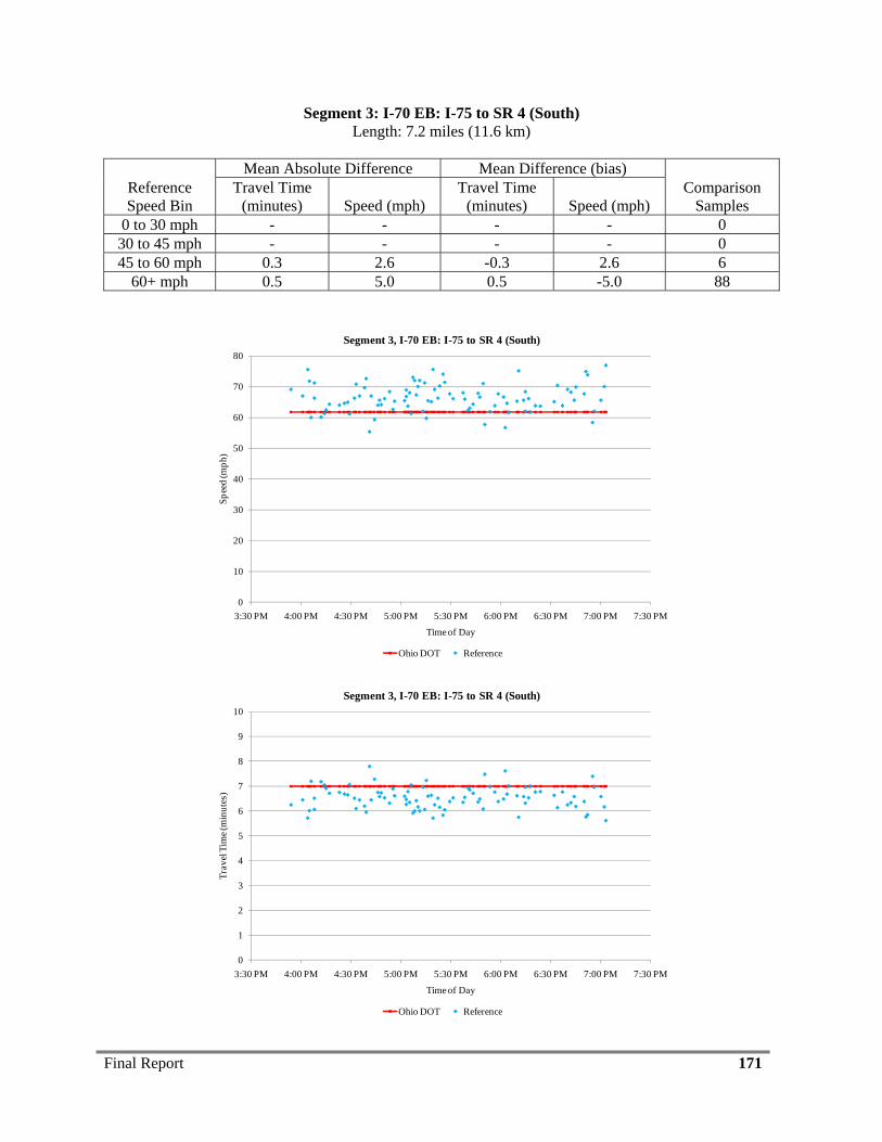
Final Report 171

Segment 3: I-70 EB: I-75 to SR 4 (South) Length: 7.2 miles (11.6 km)

Reference Speed Bin


Samples Travel Time



30 to 45 mph - - - - 0 45 to 60 mph 0.3 2.6 -0.3 2.6 6

60+ mph 0.5 5.0 0.5 -5.0 88

0

10

20

30

40

50

60

70

80


Spee

d (m

ph)

Time of Day


Ohio DOT Reference

0

1

2

3

4

5

6

7

8

9

10


Trav

el T

ime (

min

utes

)

Time of Day


Ohio DOT Reference

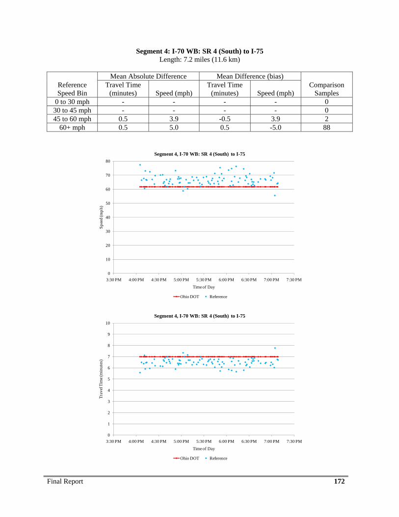
Final Report 172

Segment 4: I-70 WB: SR 4 (South) to I-75 Length: 7.2 miles (11.6 km)

Reference Speed Bin


Samples Travel Time



30 to 45 mph - - - - 0 45 to 60 mph 0.5 3.9 -0.5 3.9 2

60+ mph 0.5 5.0 0.5 -5.0 88

0

10

20

30

40

50

60

70

80


Spee

d (m

ph)

Time of Day

Segment 4, I-70 WB: SR 4 (South) to I-75

Ohio DOT Reference

0

1

2

3

4

5

6

7

8

9

10


Trav

el T

ime (

min

utes

)

Time of Day

Segment 4, I-70 WB: SR 4 (South) to I-75

Ohio DOT Reference

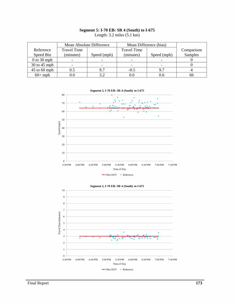
Final Report 173

Segment 5: I-70 EB: SR 4 (South) to I-675 Length: 3.2 miles (5.1 km)

Reference Speed Bin


Samples Travel Time



30 to 45 mph - - - - 0 45 to 60 mph 0.5 9.7 -0.5 9.7 4

60+ mph 0.0 3.2 0.0 0.6 66

0

10

20

30

40

50

60

70

80


Spee

d (m

ph)

Time of Day

Segment 5, I-70 EB: SR 4 (South) to I-675

Ohio DOT Reference

0

1

2

3

4

5

6

7

8

9

10


Trav

el T

ime (

min

utes

)

Time of Day

Segment 5, I-70 EB: SR 4 (South) to I-675

Ohio DOT Reference

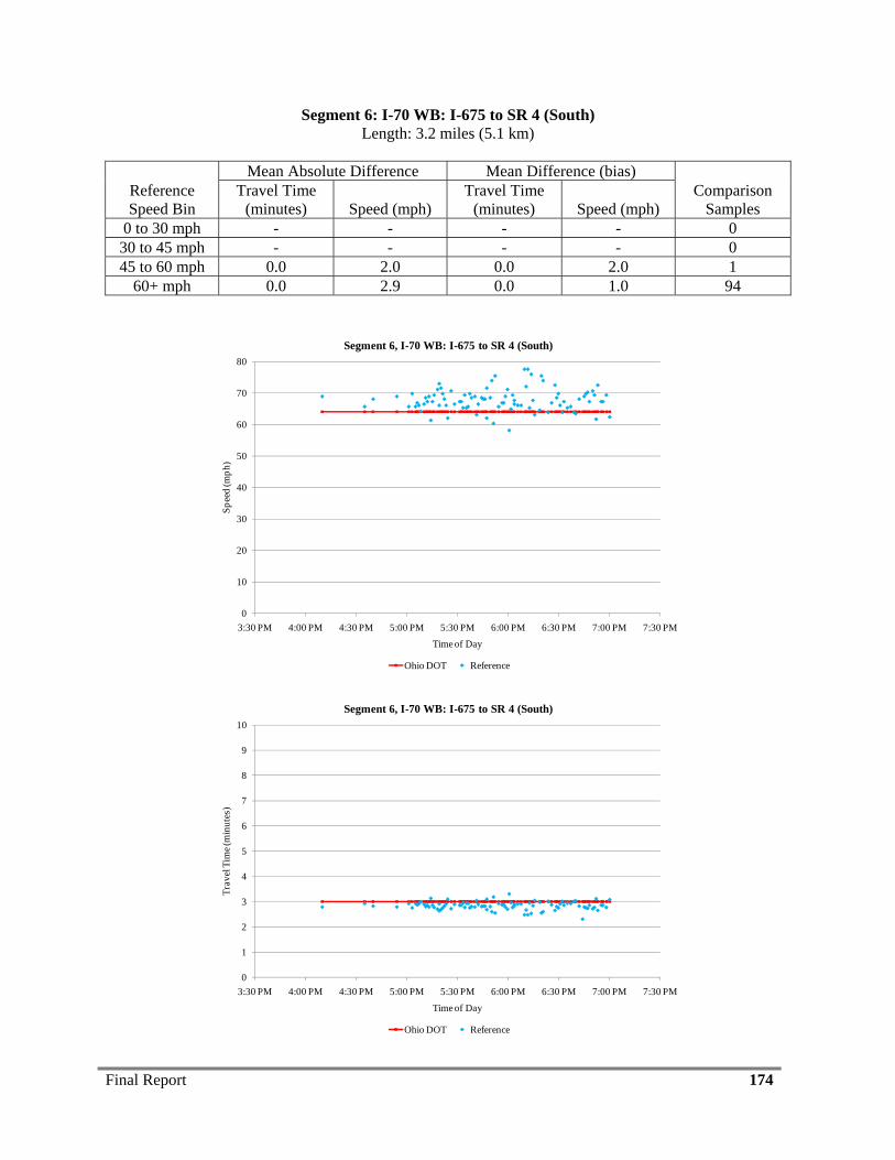
Final Report 174

Segment 6: I-70 WB: I-675 to SR 4 (South) Length: 3.2 miles (5.1 km)

Reference Speed Bin


Samples Travel Time



30 to 45 mph - - - - 0 45 to 60 mph 0.0 2.0 0.0 2.0 1

60+ mph 0.0 2.9 0.0 1.0 94

0

10

20

30

40

50

60

70

80


Spee

d (m

ph)

Time of Day

Segment 6, I-70 WB: I-675 to SR 4 (South)

Ohio DOT Reference

0

1

2

3

4

5

6

7

8

9

10


Trav

el T

ime (

min

utes

)

Time of Day

Segment 6, I-70 WB: I-675 to SR 4 (South)

Ohio DOT Reference

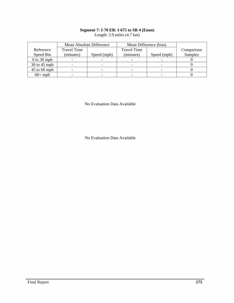
Final Report 175

Segment 7: I-70 EB: I-675 to SR 4 (Enon) Length: 2.9 miles (4.7 km)

Reference Speed Bin


Samples Travel Time



30 to 45 mph - - - - 0 45 to 60 mph - - - - 0

60+ mph - - - - 0

No Evaluation Data Available


Final Report 176

Segment 8: I-70 WB: SR 4 (Enon) to I-675 Length: 2.9 miles (4.7 km)

Reference Speed Bin


Samples Travel Time



30 to 45 mph - - - - 0 45 to 60 mph - - - - 0

60+ mph - - - - 0



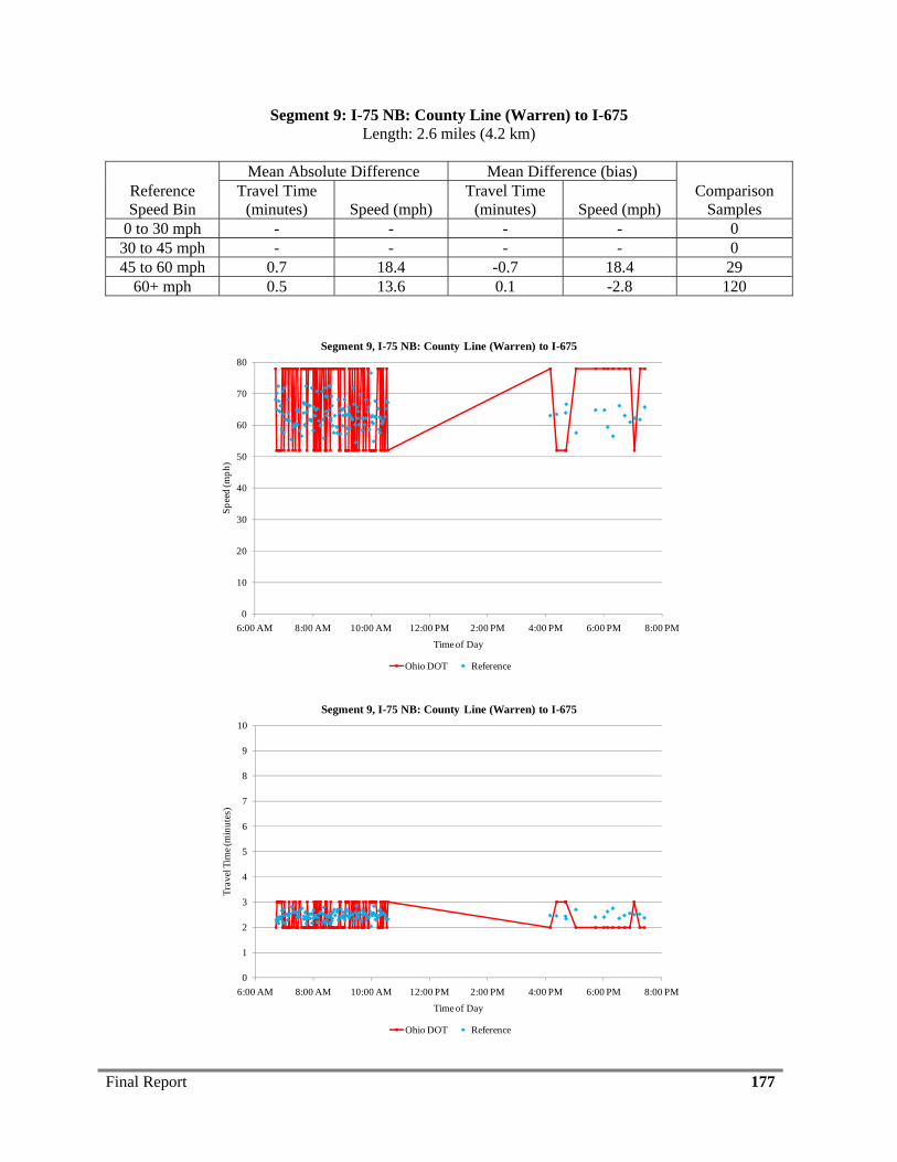
Final Report 177

Segment 9: I-75 NB: County Line (Warren) to I-675 Length: 2.6 miles (4.2 km)

Reference Speed Bin


Samples Travel Time



30 to 45 mph - - - - 0 45 to 60 mph 0.7 18.4 -0.7 18.4 29

60+ mph 0.5 13.6 0.1 -2.8 120

0

10

20

30

40

50

60

70

80


Spee

d (m

ph)

Time of Day


Ohio DOT Reference

0

1

2

3

4

5

6

7

8

9

10


Trav

el T

ime (

min

utes

)

Time of Day


Ohio DOT Reference

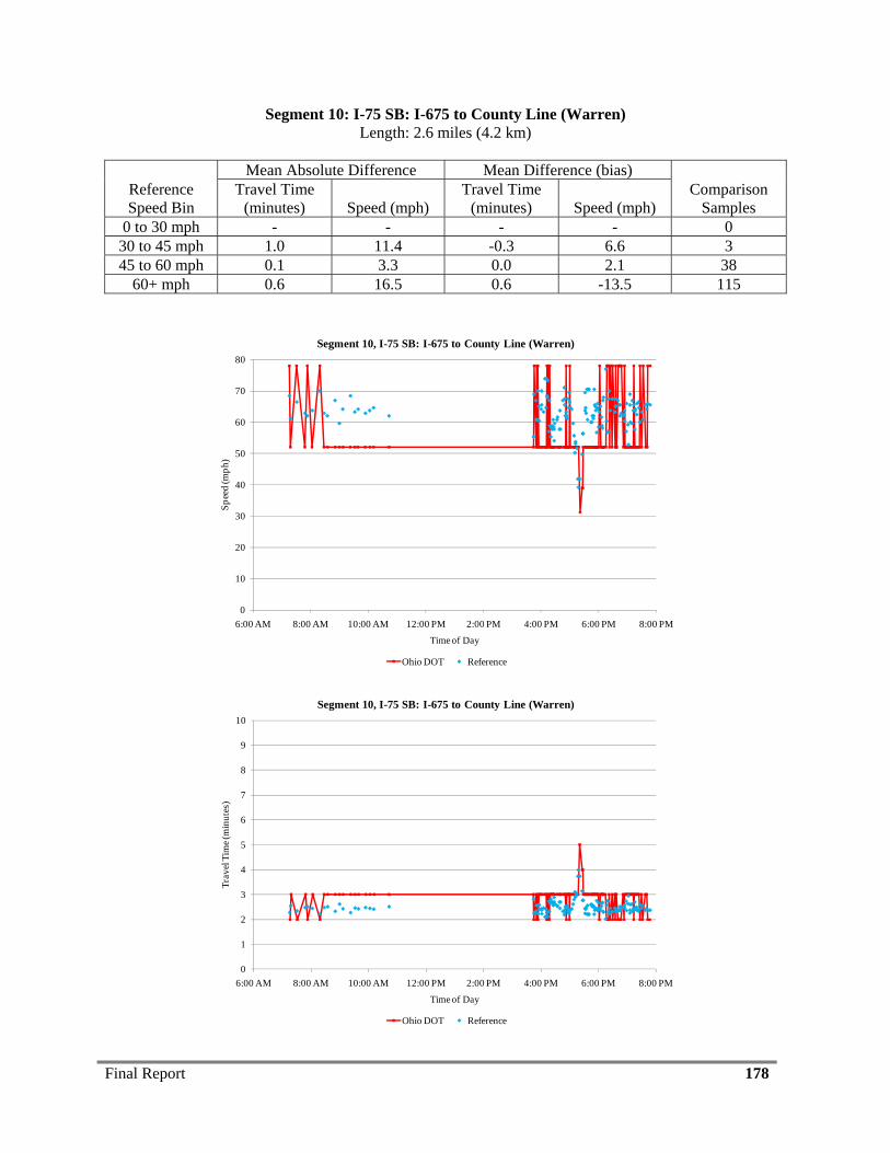
Final Report 178

Segment 10: I-75 SB: I-675 to County Line (Warren) Length: 2.6 miles (4.2 km)

Reference Speed Bin


Samples Travel Time



30 to 45 mph 1.0 11.4 -0.3 6.6 3 45 to 60 mph 0.1 3.3 0.0 2.1 38

60+ mph 0.6 16.5 0.6 -13.5 115

0

10

20

30

40

50

60

70

80


Spee

d (m

ph)

Time of Day

Segment 10, I-75 SB: I-675 to County Line (Warren)

Ohio DOT Reference

0

1

2

3

4

5

6

7

8

9

10


Trav

el T

ime (

min

utes

)

Time of Day

Segment 10, I-75 SB: I-675 to County Line (Warren)

Ohio DOT Reference

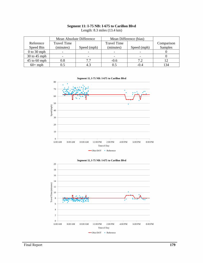
Final Report 179

Segment 11: I-75 NB: I-675 to Carillon Blvd Length: 8.3 miles (13.4 km)

Reference Speed Bin


Samples Travel Time



30 to 45 mph - - - - 0 45 to 60 mph 0.8 7.7 -0.6 7.2 12

60+ mph 0.5 4.3 0.5 -0.4 134

0

10

20

30

40

50

60

70

80


Spee

d (m

ph)

Time of Day

Segment 11, I-75 NB: I-675 to Carillon Blvd

Ohio DOT Reference

0

2

4

6

8

10

12

14

16

18

20


Trav

el T

ime (

min

utes

)

Time of Day

Segment 11, I-75 NB: I-675 to Carillon Blvd

Ohio DOT Reference

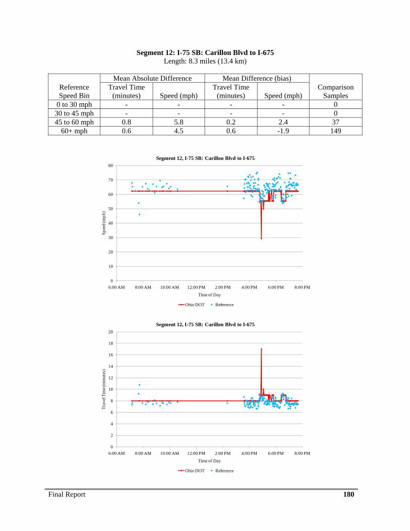
Final Report 180

Segment 12: I-75 SB: Carillon Blvd to I-675 Length: 8.3 miles (13.4 km)

Reference Speed Bin


Samples Travel Time



30 to 45 mph - - - - 0 45 to 60 mph 0.8 5.8 0.2 2.4 37

60+ mph 0.6 4.5 0.6 -1.9 149

0

10

20

30

40

50

60

70

80


Spee

d (m

ph)

Time of Day

Segment 12, I-75 SB: Carillon Blvd to I-675

Ohio DOT Reference

0

2

4

6

8

10

12

14

16

18

20


Trav

el T

ime (

min

utes

)

Time of Day

Segment 12, I-75 SB: Carillon Blvd to I-675

Ohio DOT Reference

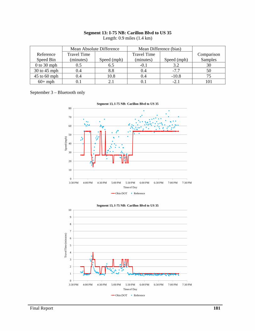
Final Report 181

Segment 13: I-75 NB: Carillon Blvd to US 35 Length: 0.9 miles (1.4 km)

Reference Speed Bin


Samples Travel Time


(minutes) Speed (mph) 0 to 30 mph 0.5 6.5 -0.1 3.2 30

30 to 45 mph 0.4 8.8 0.4 -7.7 50 45 to 60 mph 0.4 10.8 0.4 -10.8 75

60+ mph 0.1 2.1 0.1 -2.1 101 September 3 – Bluetooth only

0

10

20

30

40

50

60

70

80


Spee

d (m

ph)

Time of Day

Segment 13, I-75 NB: Carillon Blvd to US 35

Ohio DOT Reference

0

1

2

3

4

5

6

7

8

9

10


Trav

el T

ime (

min

utes

)

Time of Day


Ohio DOT Reference

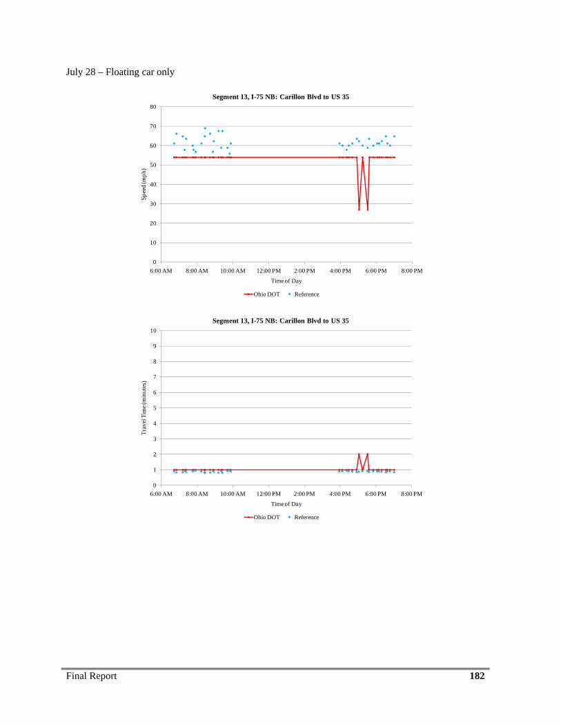
Final Report 182

July 28 – Floating car only

0

10

20

30

40

50

60

70

80


Spee

d (m

ph)

Time of Day


Ohio DOT Reference

0

1

2

3

4

5

6

7

8

9

10


Trav

el T

ime (

min

utes

)

Time of Day


Ohio DOT Reference

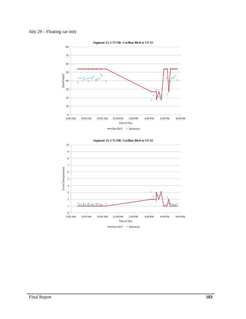
Final Report 183


0

10

20

30

40

50

60

70

80


Spee

d (m

ph)

Time of Day


Ohio DOT Reference

0

1

2

3

4

5

6

7

8

9

10


Trav

el T

ime (

min

utes

)

Time of Day


Ohio DOT Reference

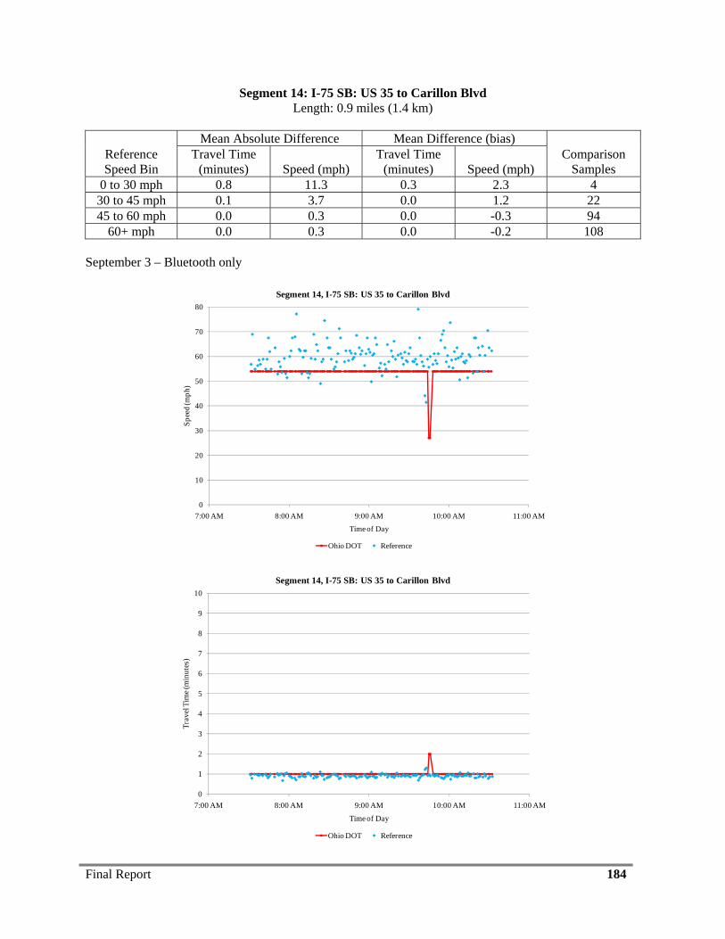
Final Report 184

Segment 14: I-75 SB: US 35 to Carillon Blvd Length: 0.9 miles (1.4 km)

Reference Speed Bin


Samples Travel Time


(minutes) Speed (mph) 0 to 30 mph 0.8 11.3 0.3 2.3 4

30 to 45 mph 0.1 3.7 0.0 1.2 22 45 to 60 mph 0.0 0.3 0.0 -0.3 94


0

10

20

30

40

50

60

70

80

7:00 AM 8:00 AM 9:00 AM 10:00 AM 11:00 AM

Spee

d (m

ph)

Time of Day

Segment 14, I-75 SB: US 35 to Carillon Blvd

Ohio DOT Reference

0

1

2

3

4

5

6

7

8

9

10

7:00 AM 8:00 AM 9:00 AM 10:00 AM 11:00 AM

Trav

el T

ime (

min

utes

)

Time of Day


Ohio DOT Reference

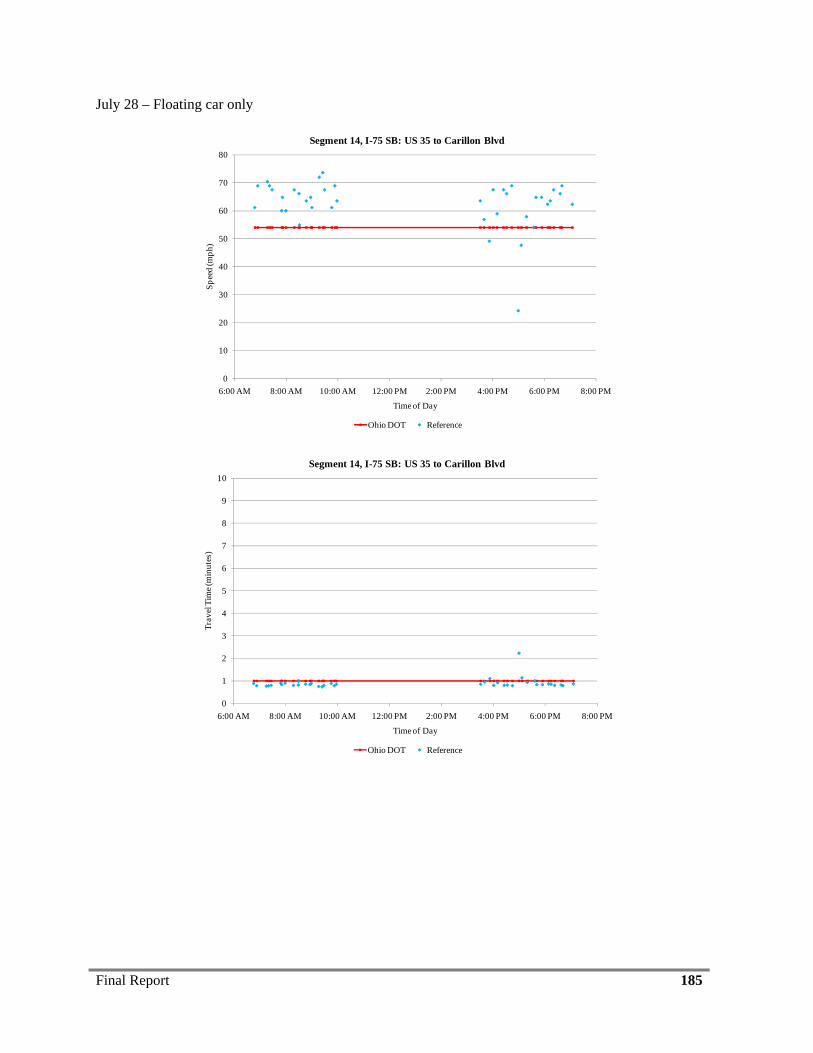
Final Report 185


0

10

20

30

40

50

60

70

80


Spee

d (m

ph)

Time of Day


Ohio DOT Reference

0

1

2

3

4

5

6

7

8

9

10


Trav

el T

ime (

min

utes

)

Time of Day


Ohio DOT Reference

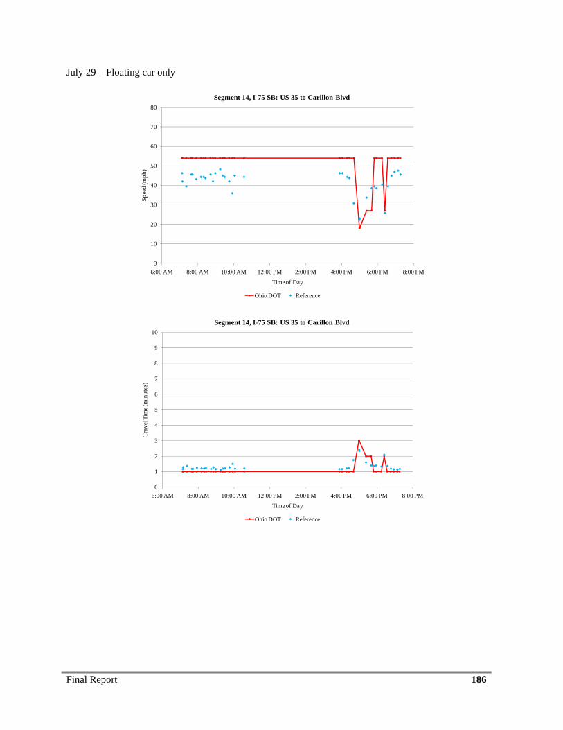
Final Report 186


0

10

20

30

40

50

60

70

80


Spee

d (m

ph)

Time of Day


Ohio DOT Reference

0

1

2

3

4

5

6

7

8

9

10


Trav

el T

ime (

min

utes

)

Time of Day


Ohio DOT Reference

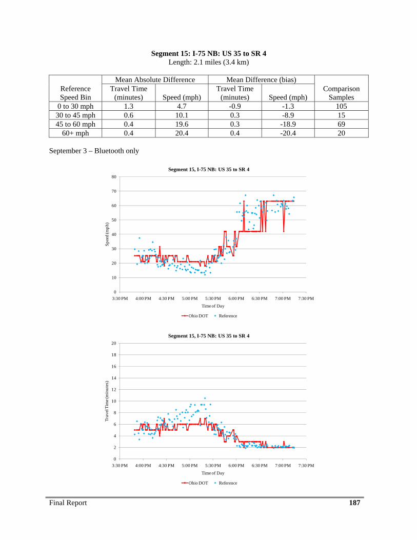
Final Report 187

Segment 15: I-75 NB: US 35 to SR 4 Length: 2.1 miles (3.4 km)

Reference Speed Bin


Samples Travel Time


(minutes) Speed (mph) 0 to 30 mph 1.3 4.7 -0.9 -1.3 105

30 to 45 mph 0.6 10.1 0.3 -8.9 15 45 to 60 mph 0.4 19.6 0.3 -18.9 69


0

10

20

30

40

50

60

70

80


Spee

d (m

ph)

Time of Day


Ohio DOT Reference

0

2

4

6

8

10

12

14

16

18

20


Trav

el T

ime (

min

utes

)

Time of Day


Ohio DOT Reference

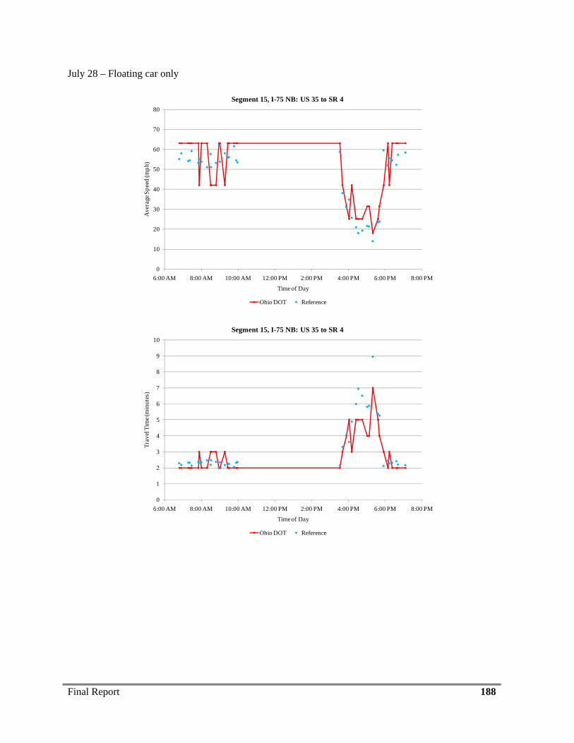
Final Report 188


0

10

20

30

40

50

60

70

80


Ave

rage

Spe

ed (m

ph)

Time of Day


Ohio DOT Reference

0

1

2

3

4

5

6

7

8

9

10


Trav

el T

ime (

min

utes

)

Time of Day


Ohio DOT Reference

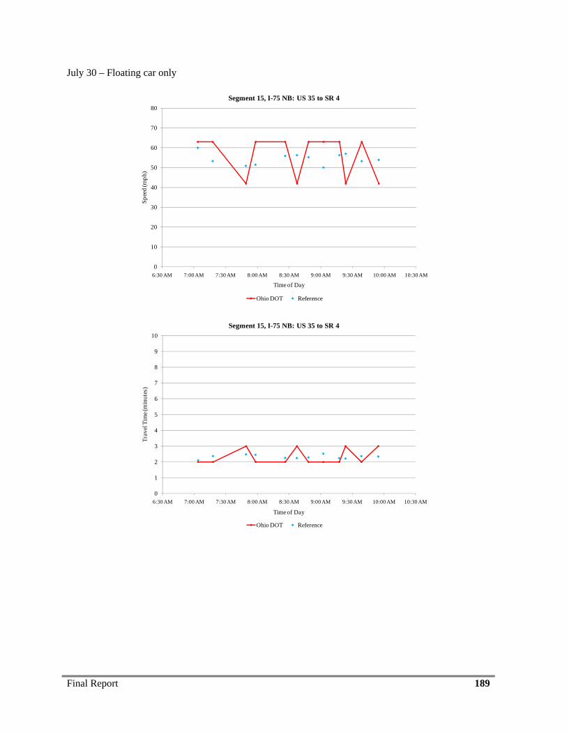
Final Report 189


0

10

20

30

40

50

60

70

80


Spee

d (m

ph)

Time of Day


Ohio DOT Reference

0

1

2

3

4

5

6

7

8

9

10


Trav

el T

ime (

min

utes

)

Time of Day


Ohio DOT Reference

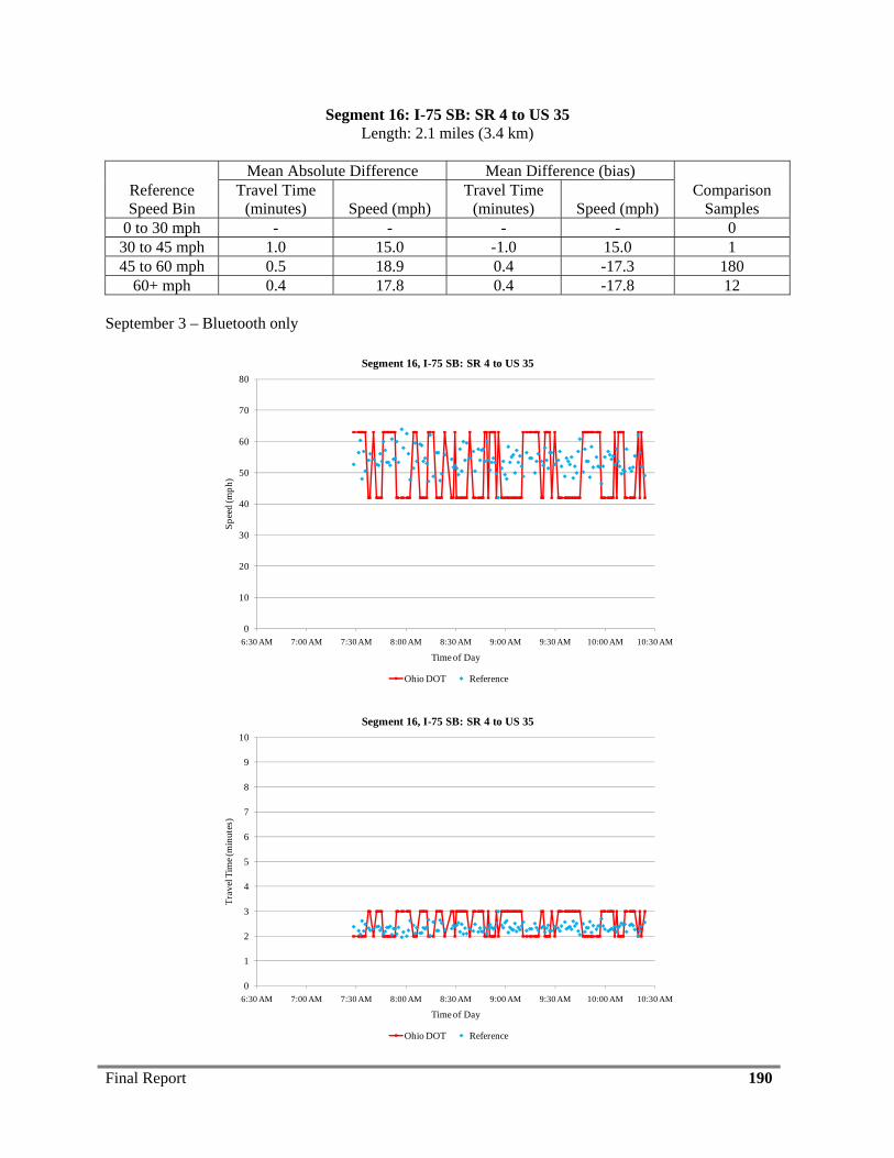
Final Report 190

Segment 16: I-75 SB: SR 4 to US 35 Length: 2.1 miles (3.4 km)

Reference Speed Bin


Samples Travel Time



30 to 45 mph 1.0 15.0 -1.0 15.0 1 45 to 60 mph 0.5 18.9 0.4 -17.3 180


0

10

20

30

40

50

60

70

80


Spee

d (m

ph)

Time of Day


Ohio DOT Reference

0

1

2

3

4

5

6

7

8

9

10


Trav

el T

ime (

min

utes

)

Time of Day


Ohio DOT Reference

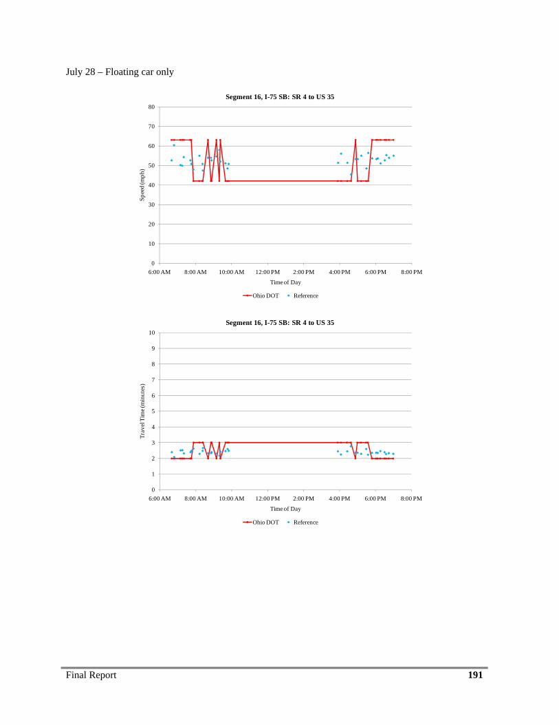
Final Report 191


0

10

20

30

40

50

60

70

80


Spee

d (m

ph)

Time of Day


Ohio DOT Reference

0

1

2

3

4

5

6

7

8

9

10


Trav

el T

ime (

min

utes

)

Time of Day


Ohio DOT Reference

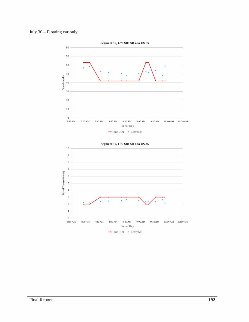
Final Report 192


0

10

20

30

40

50

60

70

80


Spee

d (m

ph)

Time of Day


Ohio DOT Reference

0

1

2

3

4

5

6

7

8

9

10


Trav

el T

ime (

min

utes

)

Time of Day


Ohio DOT Reference

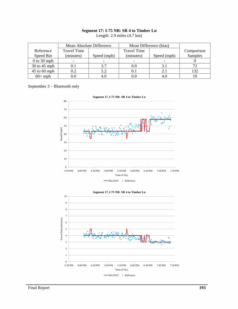
Final Report 193

Segment 17: I-75 NB: SR 4 to Timber Ln Length: 2.9 miles (4.7 km)

Reference Speed Bin


Samples Travel Time



30 to 45 mph 0.1 3.7 0.0 3.1 72 45 to 60 mph 0.2 5.2 0.1 2.1 132

60+ mph 0.0 4.0 0.0 4.0 19 September 3 – Bluetooth only

0

10

20

30

40

50

60

70

80


Spee

d (m

ph)

Time of Day

Segment 17, I-75 NB: SR 4 to Timber Ln

Ohio DOT Reference

0

1

2

3

4

5

6

7

8

9

10


Trav

el T

ime (

min

utes

)

Time of Day


Ohio DOT Reference

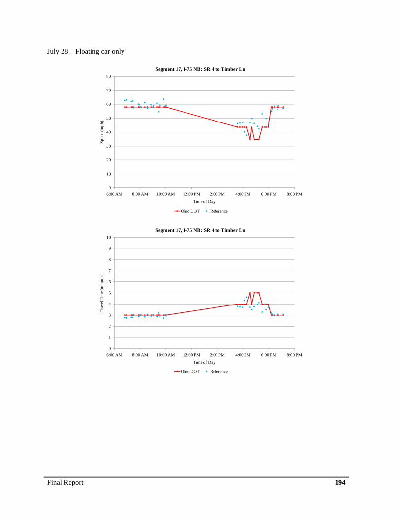
Final Report 194


0

10

20

30

40

50

60

70

80


Spee

d (m

ph)

Time of Day


Ohio DOT Reference

0

1

2

3

4

5

6

7

8

9

10


Trav

el T

ime (

min

utes

)

Time of Day


Ohio DOT Reference

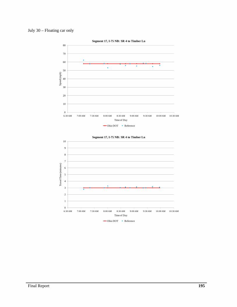
Final Report 195


0

10

20

30

40

50

60

70

80


Spee

d (m

ph)

Time of Day


Ohio DOT Reference

0

1

2

3

4

5

6

7

8

9

10


Trav

el T

ime (

min

utes

)

Time of Day


Ohio DOT Reference

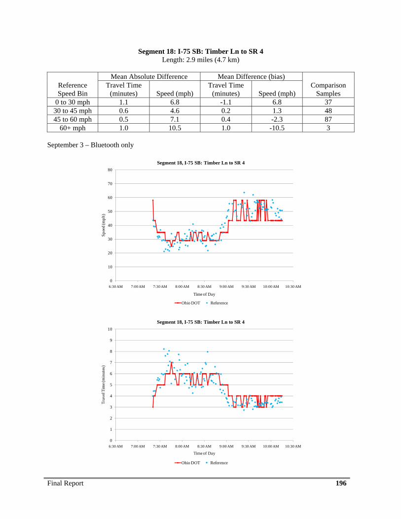
Final Report 196

Segment 18: I-75 SB: Timber Ln to SR 4 Length: 2.9 miles (4.7 km)

Reference Speed Bin


Samples Travel Time


(minutes) Speed (mph) 0 to 30 mph 1.1 6.8 -1.1 6.8 37

30 to 45 mph 0.6 4.6 0.2 1.3 48 45 to 60 mph 0.5 7.1 0.4 -2.3 87


0

10

20

30

40

50

60

70

80


Spee

d (m

ph)

Time of Day

Segment 18, I-75 SB: Timber Ln to SR 4

Ohio DOT Reference

0

1

2

3

4

5

6

7

8

9

10


Trav

el T

ime (

min

utes

)

Time of Day


Ohio DOT Reference

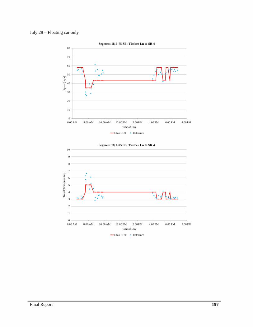
Final Report 197


0

10

20

30

40

50

60

70

80


Spee

d (m

ph)

Time of Day


Ohio DOT Reference

0

1

2

3

4

5

6

7

8

9

10


Trav

el T

ime (

min

utes

)

Time of Day


Ohio DOT Reference

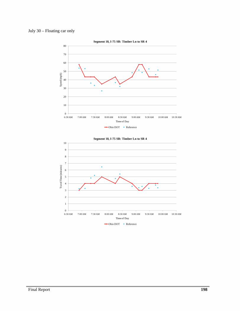
Final Report 198


0

10

20

30

40

50

60

70

80


Spee

d (m

ph)

Time of Day


Ohio DOT Reference

0

1

2

3

4

5

6

7

8

9

10


Trav

el T

ime (

min

utes

)

Time of Day


Ohio DOT Reference

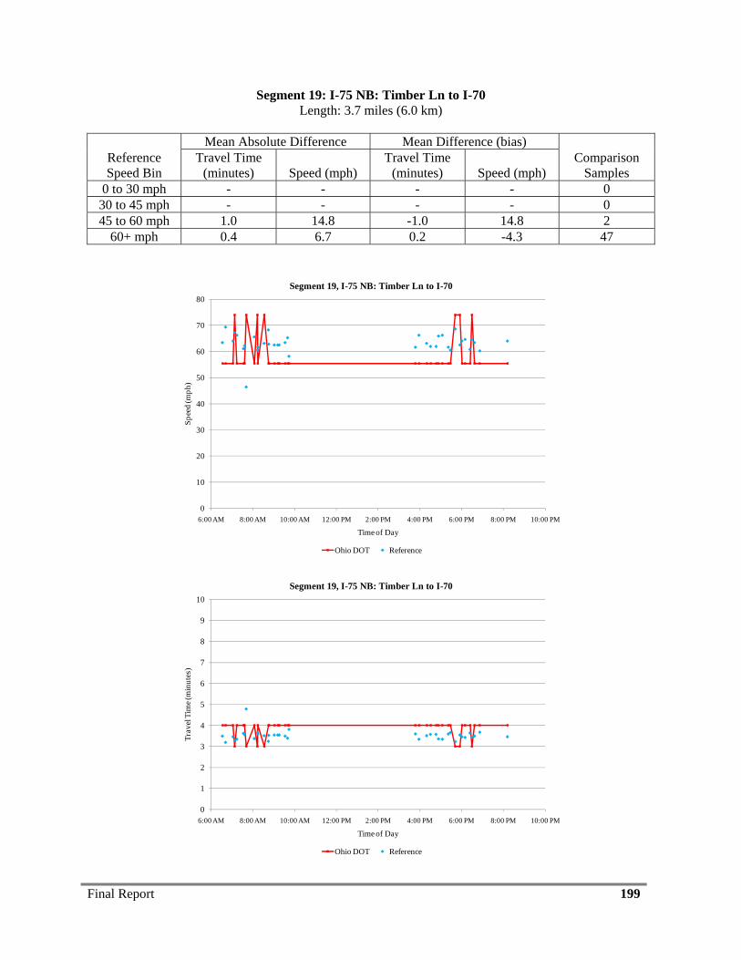
Final Report 199

Segment 19: I-75 NB: Timber Ln to I-70 Length: 3.7 miles (6.0 km)

Reference Speed Bin


Samples Travel Time



30 to 45 mph - - - - 0 45 to 60 mph 1.0 14.8 -1.0 14.8 2

60+ mph 0.4 6.7 0.2 -4.3 47

0

10

20

30

40

50

60

70

80


Spee

d (m

ph)

Time of Day

Segment 19, I-75 NB: Timber Ln to I-70

Ohio DOT Reference

0

1

2

3

4

5

6

7

8

9

10


Trav

el T

ime (

min

utes

)

Time of Day

Segment 19, I-75 NB: Timber Ln to I-70

Ohio DOT Reference

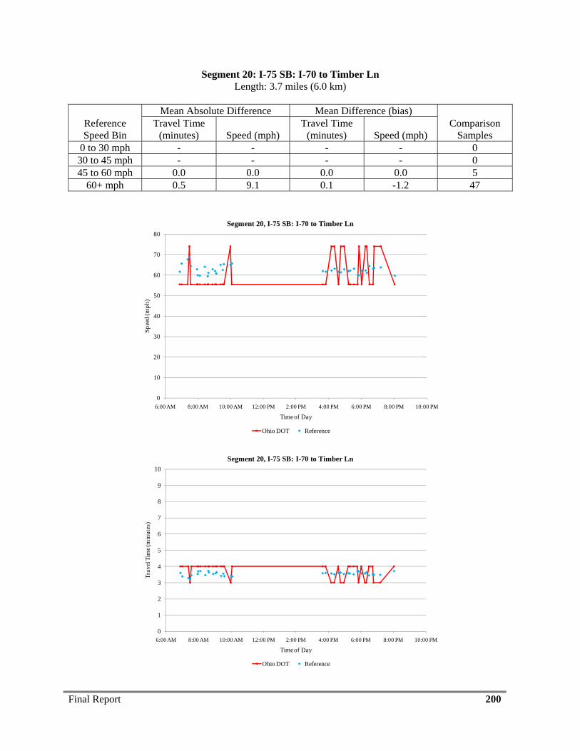
Final Report 200

Segment 20: I-75 SB: I-70 to Timber Ln Length: 3.7 miles (6.0 km)

Reference Speed Bin


Samples Travel Time



30 to 45 mph - - - - 0 45 to 60 mph 0.0 0.0 0.0 0.0 5

60+ mph 0.5 9.1 0.1 -1.2 47

0

10

20

30

40

50

60

70

80


Spee

d (m

ph)

Time of Day

Segment 20, I-75 SB: I-70 to Timber Ln

Ohio DOT Reference

0

1

2

3

4

5

6

7

8

9

10


Trav

el T

ime (

min

utes

)

Time of Day

Segment 20, I-75 SB: I-70 to Timber Ln

Ohio DOT Reference

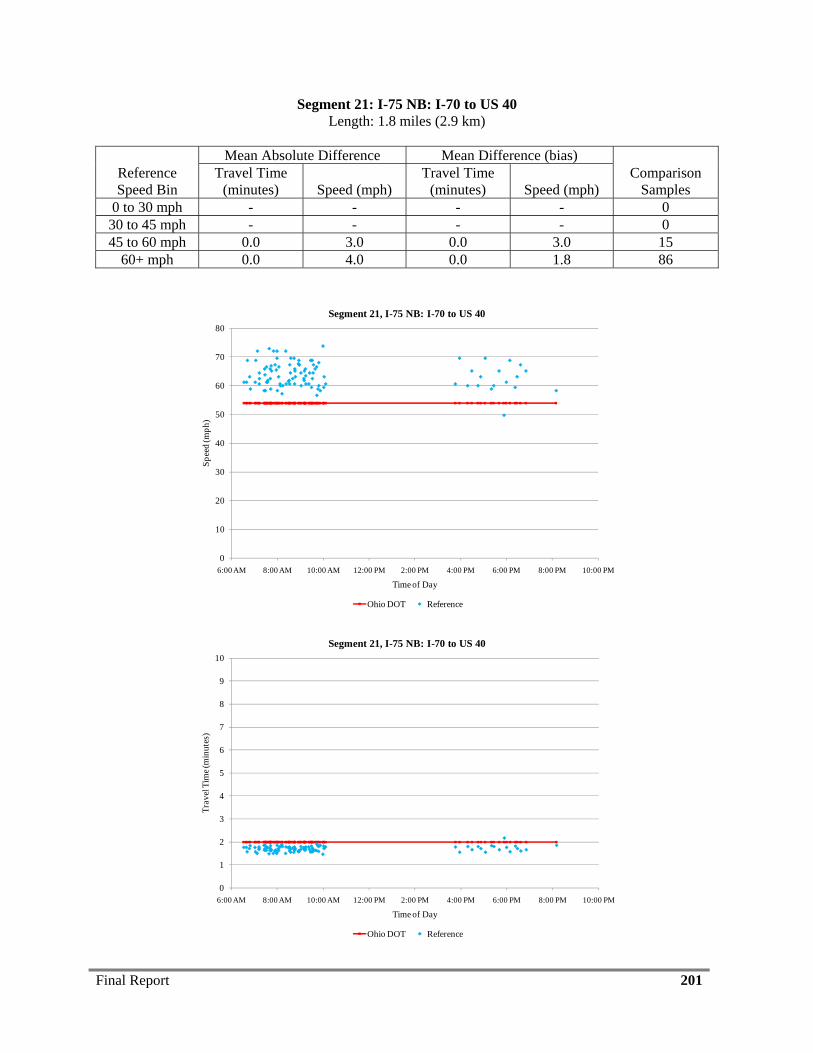
Final Report 201

Segment 21: I-75 NB: I-70 to US 40 Length: 1.8 miles (2.9 km)

Reference Speed Bin


Samples Travel Time



30 to 45 mph - - - - 0 45 to 60 mph 0.0 3.0 0.0 3.0 15

60+ mph 0.0 4.0 0.0 1.8 86

0

10

20

30

40

50

60

70

80


Spee

d (m

ph)

Time of Day


Ohio DOT Reference

0

1

2

3

4

5

6

7

8

9

10


Trav

el T

ime (

min

utes

)

Time of Day


Ohio DOT Reference

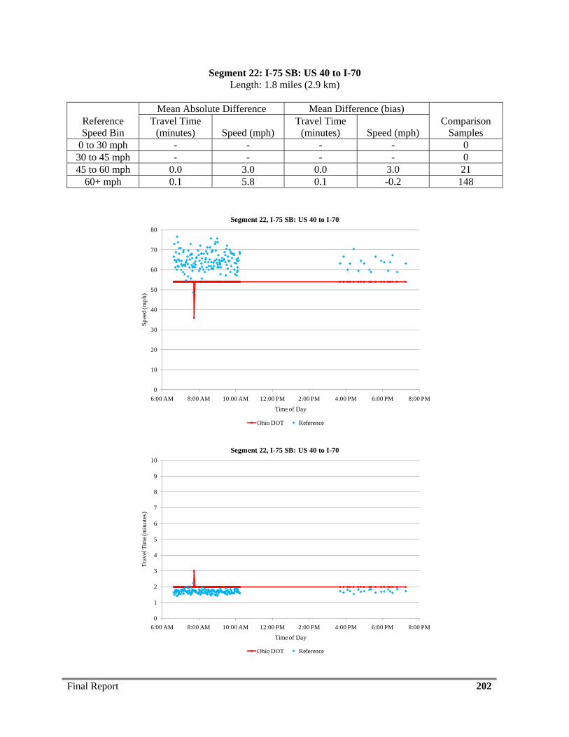
Final Report 202

Segment 22: I-75 SB: US 40 to I-70 Length: 1.8 miles (2.9 km)

Reference Speed Bin


Samples Travel Time



30 to 45 mph - - - - 0 45 to 60 mph 0.0 3.0 0.0 3.0 21

60+ mph 0.1 5.8 0.1 -0.2 148

0

10

20

30

40

50

60

70

80


Spee

d (m

ph)

Time of Day

Segment 22, I-75 SB: US 40 to I-70

Ohio DOT Reference

0

1

2

3

4

5

6

7

8

9

10


Trav

el T

ime (

min

utes

)

Time of Day


Ohio DOT Reference

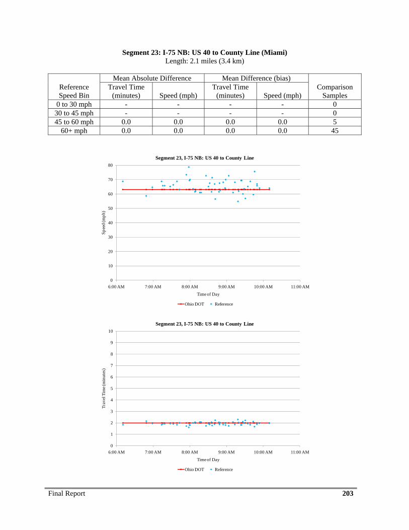
Final Report 203

Segment 23: I-75 NB: US 40 to County Line (Miami) Length: 2.1 miles (3.4 km)

Reference Speed Bin


Samples Travel Time



30 to 45 mph - - - - 0 45 to 60 mph 0.0 0.0 0.0 0.0 5

60+ mph 0.0 0.0 0.0 0.0 45

0

10

20

30

40

50

60

70

80

6:00 AM 7:00 AM 8:00 AM 9:00 AM 10:00 AM 11:00 AM

Spee

d (m

ph)

Time of Day

Segment 23, I-75 NB: US 40 to County Line

Ohio DOT Reference

0

1

2

3

4

5

6

7

8

9

10

6:00 AM 7:00 AM 8:00 AM 9:00 AM 10:00 AM 11:00 AM

Trav

el T

ime (

min

utes

)

Time of Day

Segment 23, I-75 NB: US 40 to County Line

Ohio DOT Reference

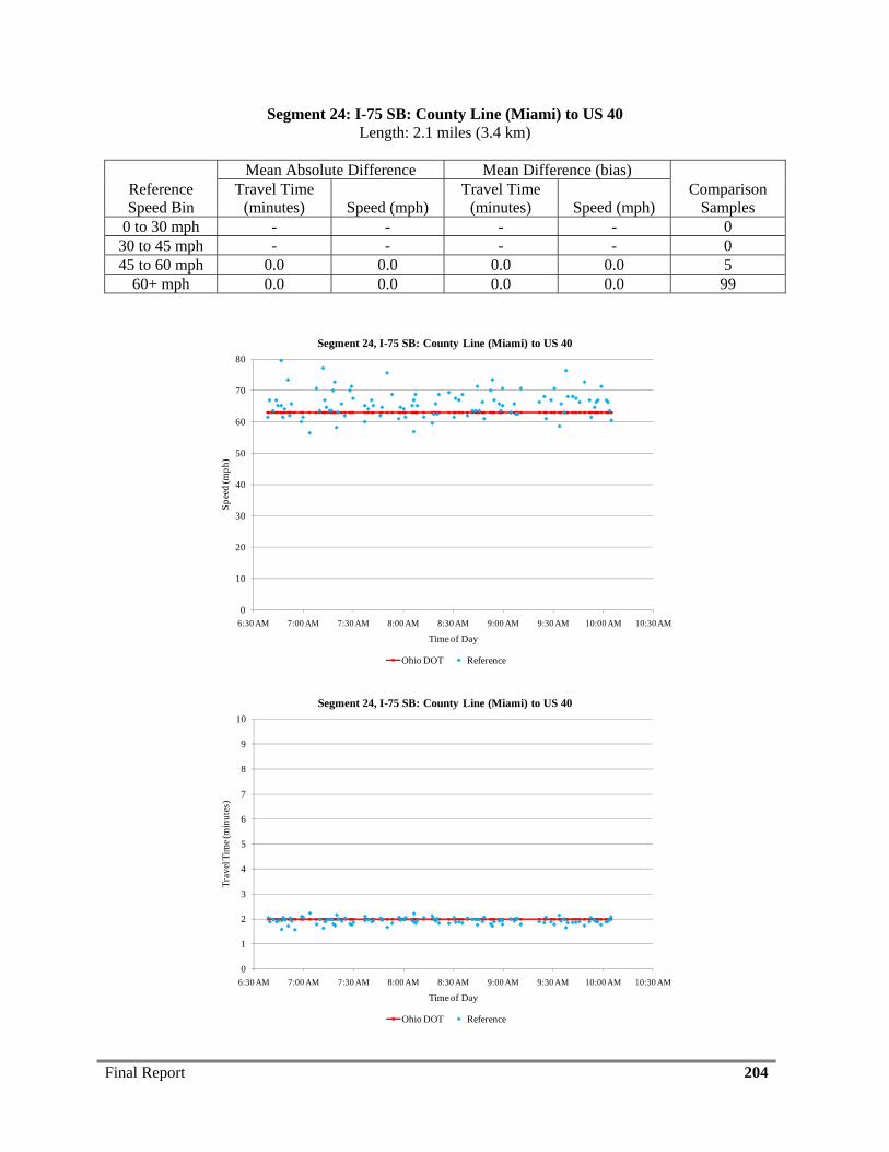
Final Report 204

Segment 24: I-75 SB: County Line (Miami) to US 40 Length: 2.1 miles (3.4 km)

Reference Speed Bin


Samples Travel Time



30 to 45 mph - - - - 0 45 to 60 mph 0.0 0.0 0.0 0.0 5

60+ mph 0.0 0.0 0.0 0.0 99

0

10

20

30

40

50

60

70

80


Spee

d (m

ph)

Time of Day

Segment 24, I-75 SB: County Line (Miami) to US 40

Ohio DOT Reference

0

1

2

3

4

5

6

7

8

9

10


Trav

el T

ime (

min

utes

)

Time of Day

Segment 24, I-75 SB: County Line (Miami) to US 40

Ohio DOT Reference

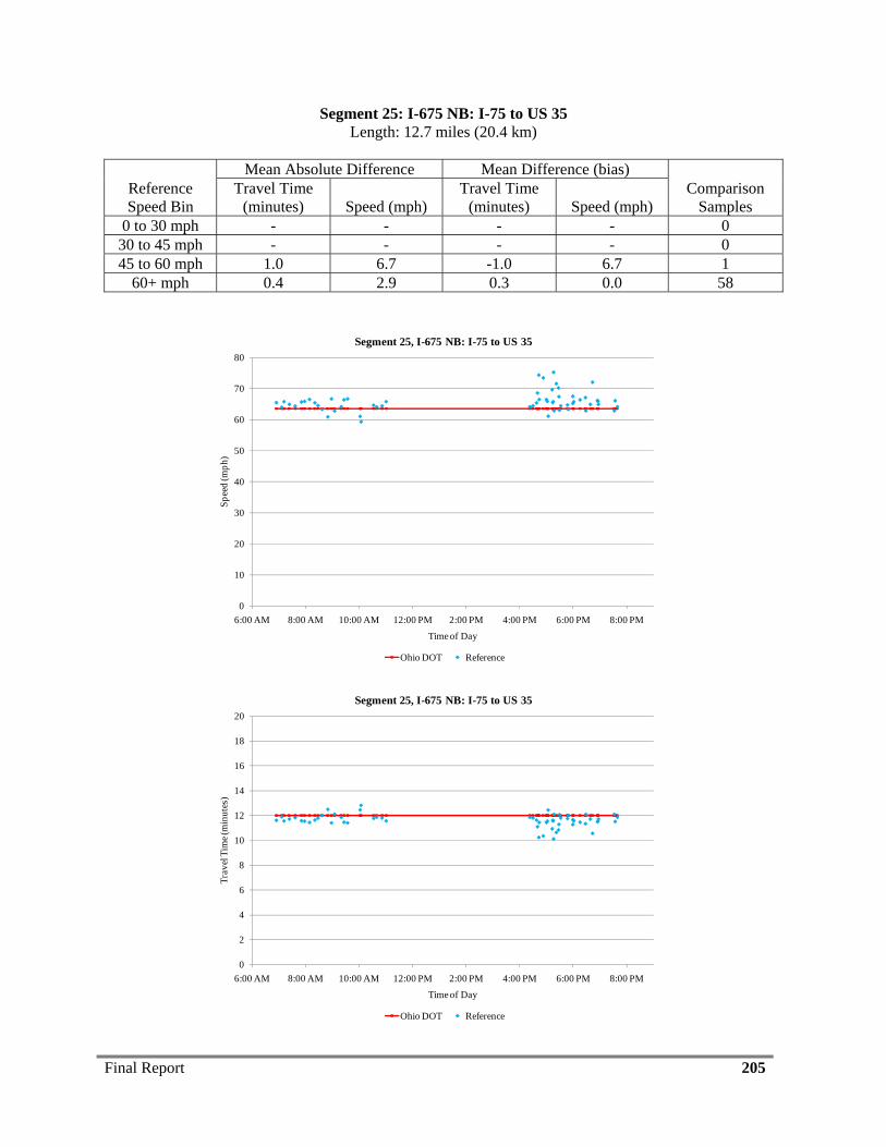
Final Report 205


Reference Speed Bin


Samples Travel Time



30 to 45 mph - - - - 0 45 to 60 mph 1.0 6.7 -1.0 6.7 1

60+ mph 0.4 2.9 0.3 0.0 58

0

10

20

30

40

50

60

70

80


Spee

d (m

ph)

Time of Day


Ohio DOT Reference

0

2

4

6

8

10

12

14

16

18

20


Trav

el T

ime (

min

utes

)

Time of Day


Ohio DOT Reference

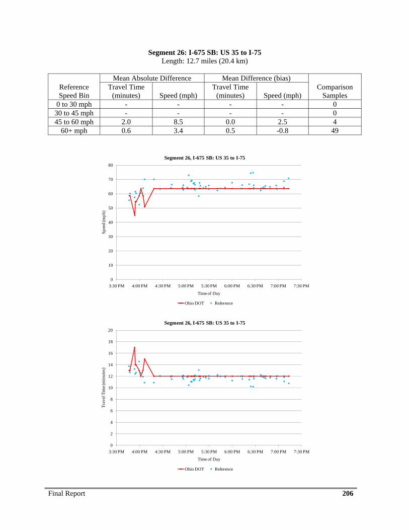
Final Report 206


Reference Speed Bin


Samples Travel Time



30 to 45 mph - - - - 0 45 to 60 mph 2.0 8.5 0.0 2.5 4

60+ mph 0.6 3.4 0.5 -0.8 49

0

10

20

30

40

50

60

70

80


Spee

d (m

ph)

Time of Day


Ohio DOT Reference

0

2

4

6

8

10

12

14

16

18

20


Trav

el T

ime (

min

utes

)

Time of Day


Ohio DOT Reference

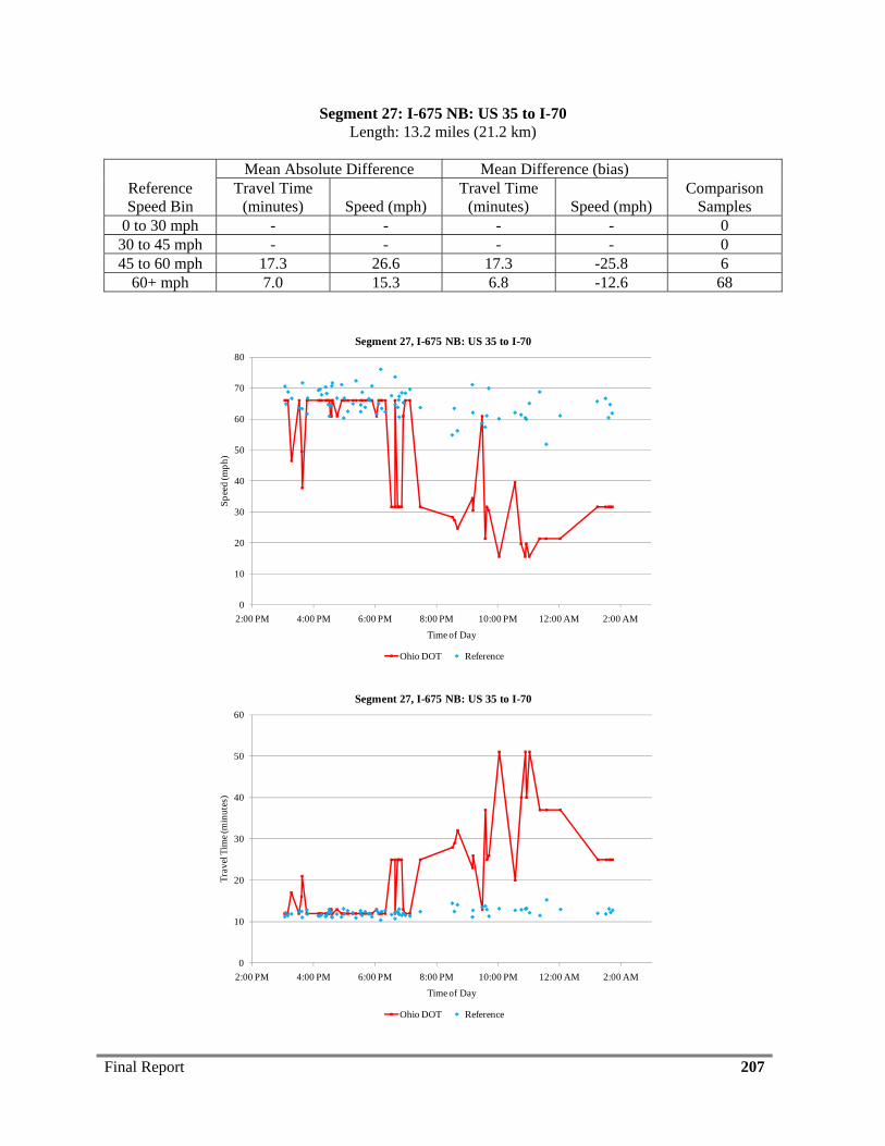
Final Report 207

Segment 27: I-675 NB: US 35 to I-70 Length: 13.2 miles (21.2 km)

Reference Speed Bin


Samples Travel Time



30 to 45 mph - - - - 0 45 to 60 mph 17.3 26.6 17.3 -25.8 6

60+ mph 7.0 15.3 6.8 -12.6 68

0

10

20

30

40

50

60

70

80

2:00 PM 4:00 PM 6:00 PM 8:00 PM 10:00 PM 12:00 AM 2:00 AM

Spee

d (m

ph)

Time of Day


Ohio DOT Reference

0

10

20

30

40

50

60

2:00 PM 4:00 PM 6:00 PM 8:00 PM 10:00 PM 12:00 AM 2:00 AM

Trav

el T

ime (

min

utes

)

Time of Day


Ohio DOT Reference

Final Report 208

Segment 28: I-675 SB: I-70 to US 35 Length: 13.2 miles (21.2 km)

Reference Speed Bin


Samples Travel Time



30 to 45 mph - - - - 0 45 to 60 mph 32.5 34.5 32.1 -32.4 11

60+ mph 5.1 11.6 5.0 -8.8 68

0

10

20

30

40

50

60

70

80

2:00 PM 4:00 PM 6:00 PM 8:00 PM 10:00 PM 12:00 AM 2:00 AM

Spee

d (m

ph)

Time of Day


Ohio DOT Reference

0

10

20

30

40

50

60

70

80

2:00 PM 4:00 PM 6:00 PM 8:00 PM 10:00 PM 12:00 AM 2:00 AM

Trav

el T

ime (

min

utes

)

Time of Day


Ohio DOT Reference

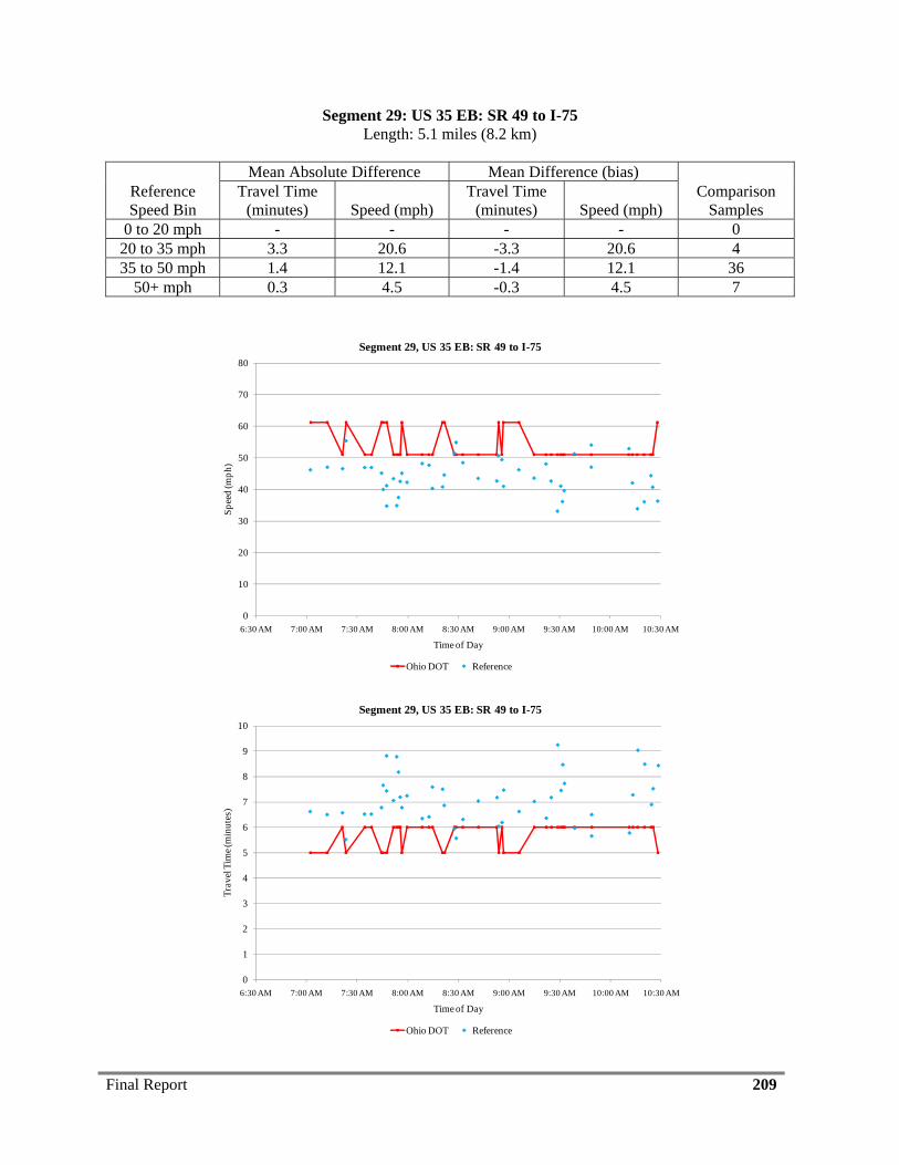
Final Report 209

Segment 29: US 35 EB: SR 49 to I-75 Length: 5.1 miles (8.2 km)

Reference Speed Bin


Samples Travel Time



20 to 35 mph 3.3 20.6 -3.3 20.6 4 35 to 50 mph 1.4 12.1 -1.4 12.1 36

50+ mph 0.3 4.5 -0.3 4.5 7

0

10

20

30

40

50

60

70

80


Spee

d (m

ph)

Time of Day


Ohio DOT Reference

0

1

2

3

4

5

6

7

8

9

10


Trav

el T

ime (

min

utes

)

Time of Day


Ohio DOT Reference

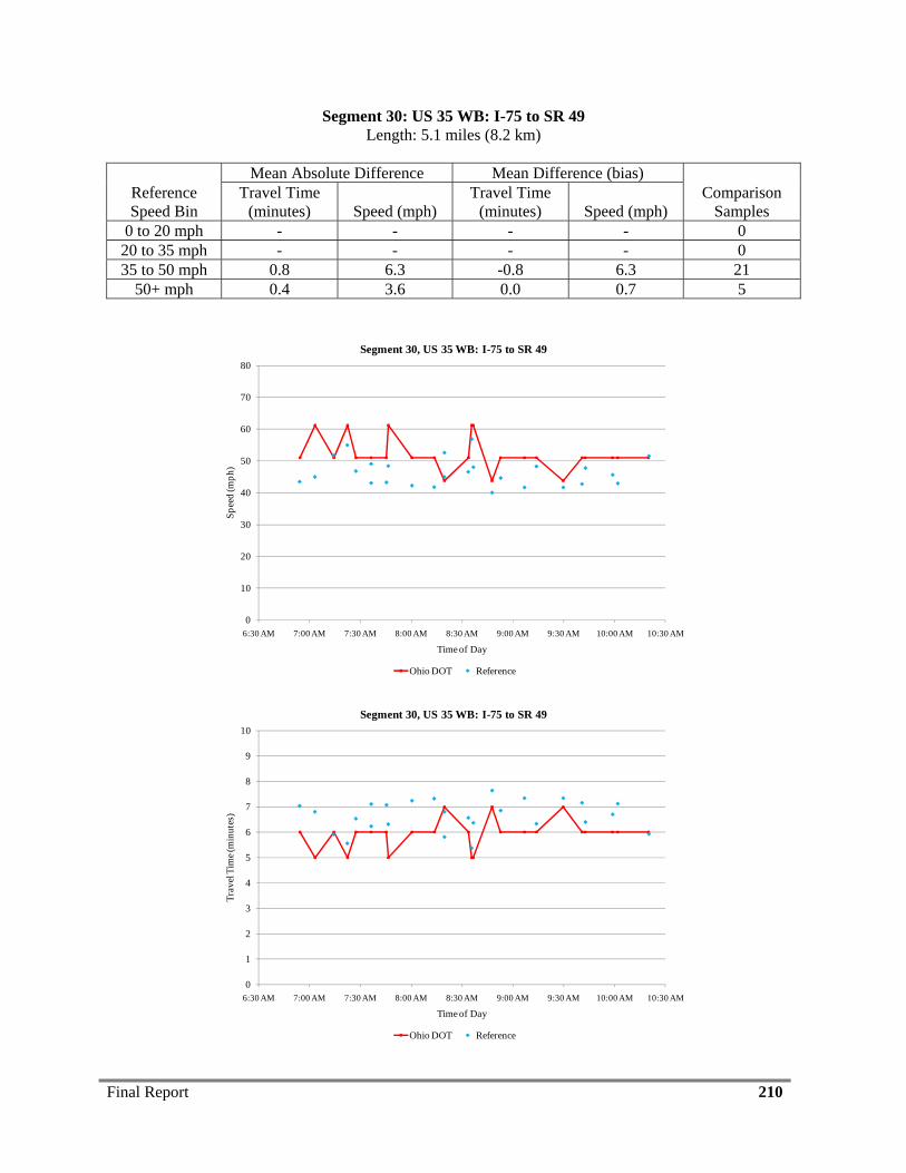
Final Report 210

Segment 30: US 35 WB: I-75 to SR 49 Length: 5.1 miles (8.2 km)

Reference Speed Bin


Samples Travel Time



20 to 35 mph - - - - 0 35 to 50 mph 0.8 6.3 -0.8 6.3 21

50+ mph 0.4 3.6 0.0 0.7 5

0

10

20

30

40

50

60

70

80


Spee

d (m

ph)

Time of Day


Ohio DOT Reference

0

1

2

3

4

5

6

7

8

9

10


Trav

el T

ime (

min

utes

)

Time of Day


Ohio DOT Reference

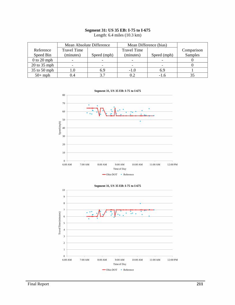
Final Report 211

Segment 31: US 35 EB: I-75 to I-675 Length: 6.4 miles (10.3 km)

Reference Speed Bin


Samples Travel Time



20 to 35 mph - - - - 0 35 to 50 mph 1.0 6.9 -1.0 6.9 1

50+ mph 0.4 3.7 0.2 -1.6 35

0

10

20

30

40

50

60

70

80

6:00 AM 7:00 AM 8:00 AM 9:00 AM 10:00 AM 11:00 AM 12:00 PM

Spee

d (m

ph)

Time of Day

Segment 31, US 35 EB: I-75 to I-675

Ohio DOT Reference

0

1

2

3

4

5

6

7

8

9

10

6:00 AM 7:00 AM 8:00 AM 9:00 AM 10:00 AM 11:00 AM 12:00 PM

Trav

el T

ime (

min

utes

)

Time of Day

Segment 31, US 35 EB: I-75 to I-675

Ohio DOT Reference

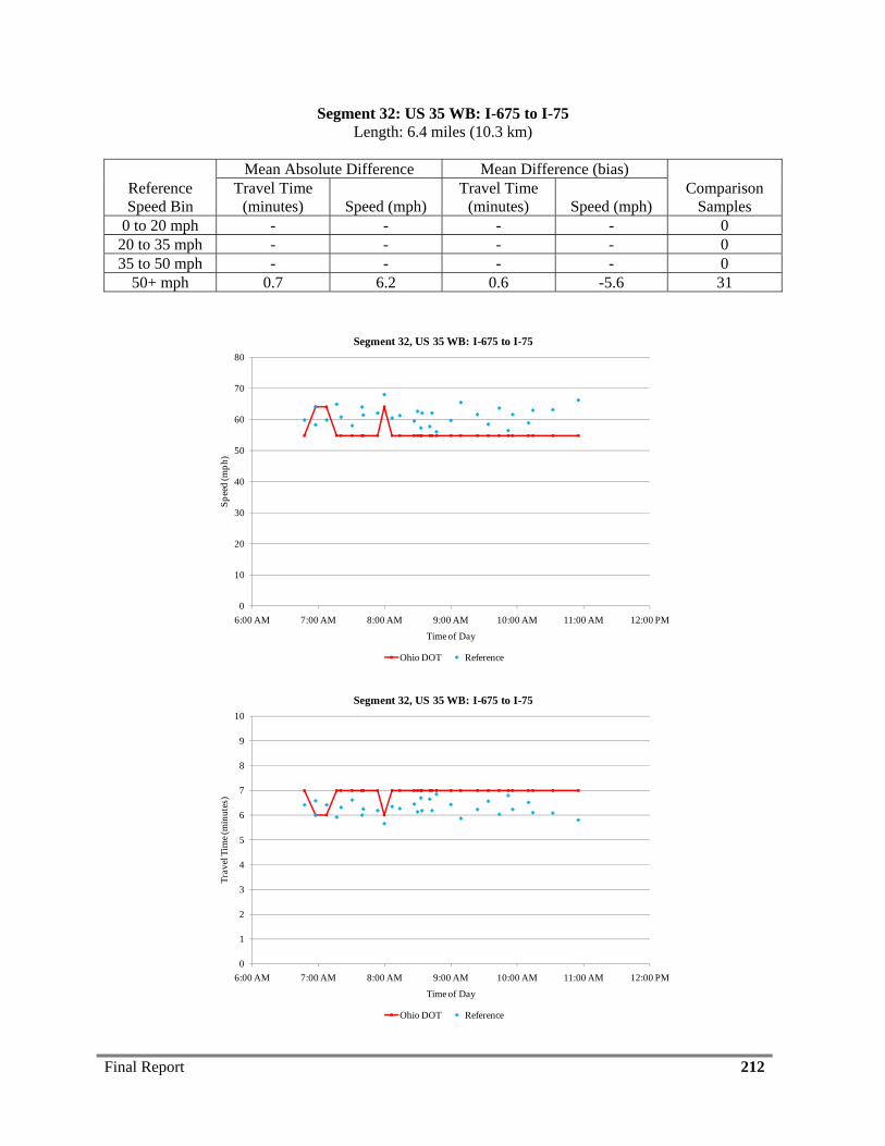
Final Report 212

Segment 32: US 35 WB: I-675 to I-75 Length: 6.4 miles (10.3 km)

Reference Speed Bin


Samples Travel Time



20 to 35 mph - - - - 0 35 to 50 mph - - - - 0

50+ mph 0.7 6.2 0.6 -5.6 31

0

10

20

30

40

50

60

70

80

6:00 AM 7:00 AM 8:00 AM 9:00 AM 10:00 AM 11:00 AM 12:00 PM

Spee

d (m

ph)

Time of Day

Segment 32, US 35 WB: I-675 to I-75

Ohio DOT Reference

0

1

2

3

4

5

6

7

8

9

10

6:00 AM 7:00 AM 8:00 AM 9:00 AM 10:00 AM 11:00 AM 12:00 PM

Trav

el T

ime (

min

utes

)

Time of Day

Segment 32, US 35 WB: I-675 to I-75

Ohio DOT Reference

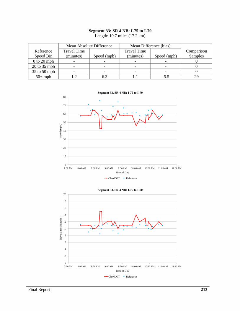
Final Report 213

Segment 33: SR 4 NB: I-75 to I-70 Length: 10.7 miles (17.2 km)

Reference Speed Bin


Samples Travel Time



20 to 35 mph - - - - 0 35 to 50 mph - - - - 0

50+ mph 1.2 6.3 1.1 -5.5 29

0

10

20

30

40

50

60

70

80


Spee

d (m

ph)

Time of Day

Segment 33, SR 4 NB: I-75 to I-70

Ohio DOT Reference

0

2

4

6

8

10

12

14

16

18

20


Trav

el T

ime (

min

utes

)

Time of Day

Segment 33, SR 4 NB: I-75 to I-70

Ohio DOT Reference

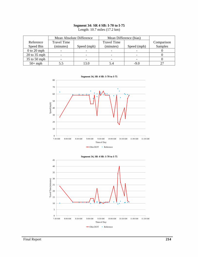
Final Report 214

Segment 34: SR 4 SB: I-70 to I-75 Length: 10.7 miles (17.2 km)

Reference Speed Bin


Samples Travel Time



20 to 35 mph - - - - 0 35 to 50 mph - - - - 0

50+ mph 5.5 13.0 5.4 -9.0 27

0

10

20

30

40

50

60

70

80


Spee

d (m

ph)

Time of Day

Segment 34, SR 4 SB: I-70 to I-75

Ohio DOT Reference

0

5

10

15

20

25

30

35

40

45


Trav

el T

ime (

min

utes

)

Time of Day

Segment 34, SR 4 SB: I-70 to I-75

Ohio DOT Reference

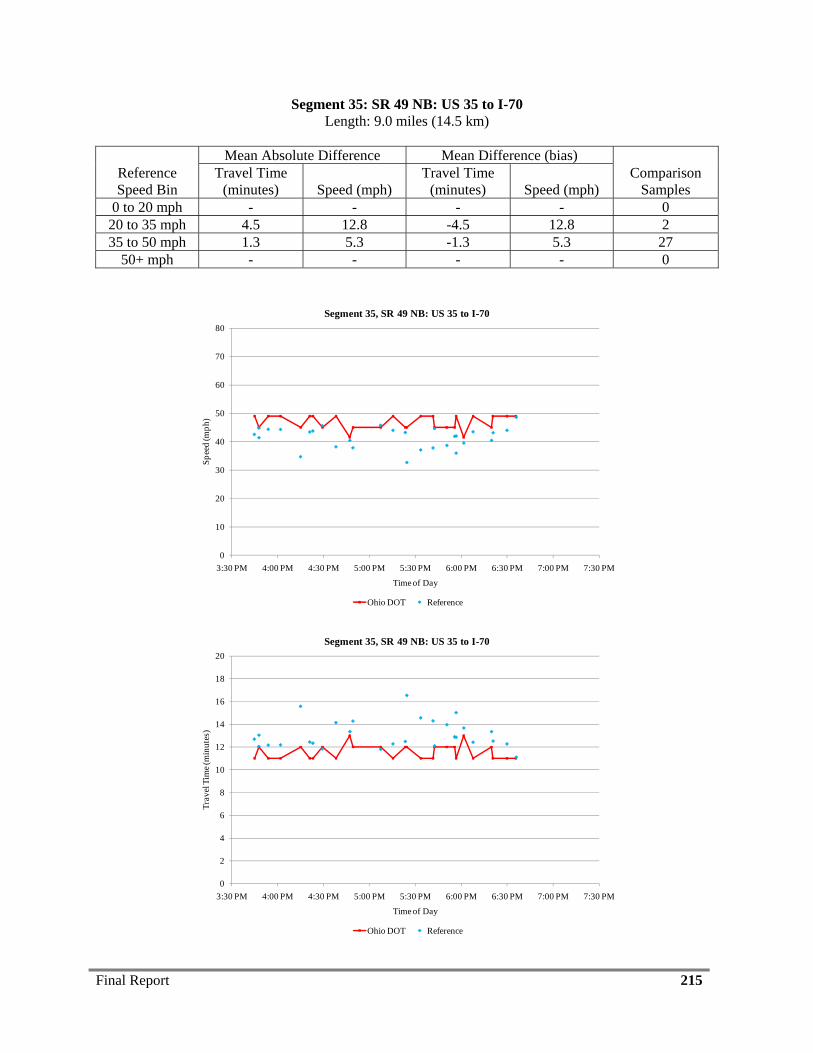
Final Report 215

Segment 35: SR 49 NB: US 35 to I-70 Length: 9.0 miles (14.5 km)

Reference Speed Bin


Samples Travel Time



20 to 35 mph 4.5 12.8 -4.5 12.8 2 35 to 50 mph 1.3 5.3 -1.3 5.3 27

50+ mph - - - - 0

0

10

20

30

40

50

60

70

80


Spee

d (m

ph)

Time of Day

Segment 35, SR 49 NB: US 35 to I-70

Ohio DOT Reference

0

2

4

6

8

10

12

14

16

18

20


Trav

el T

ime (

min

utes

)

Time of Day

Segment 35, SR 49 NB: US 35 to I-70

Ohio DOT Reference

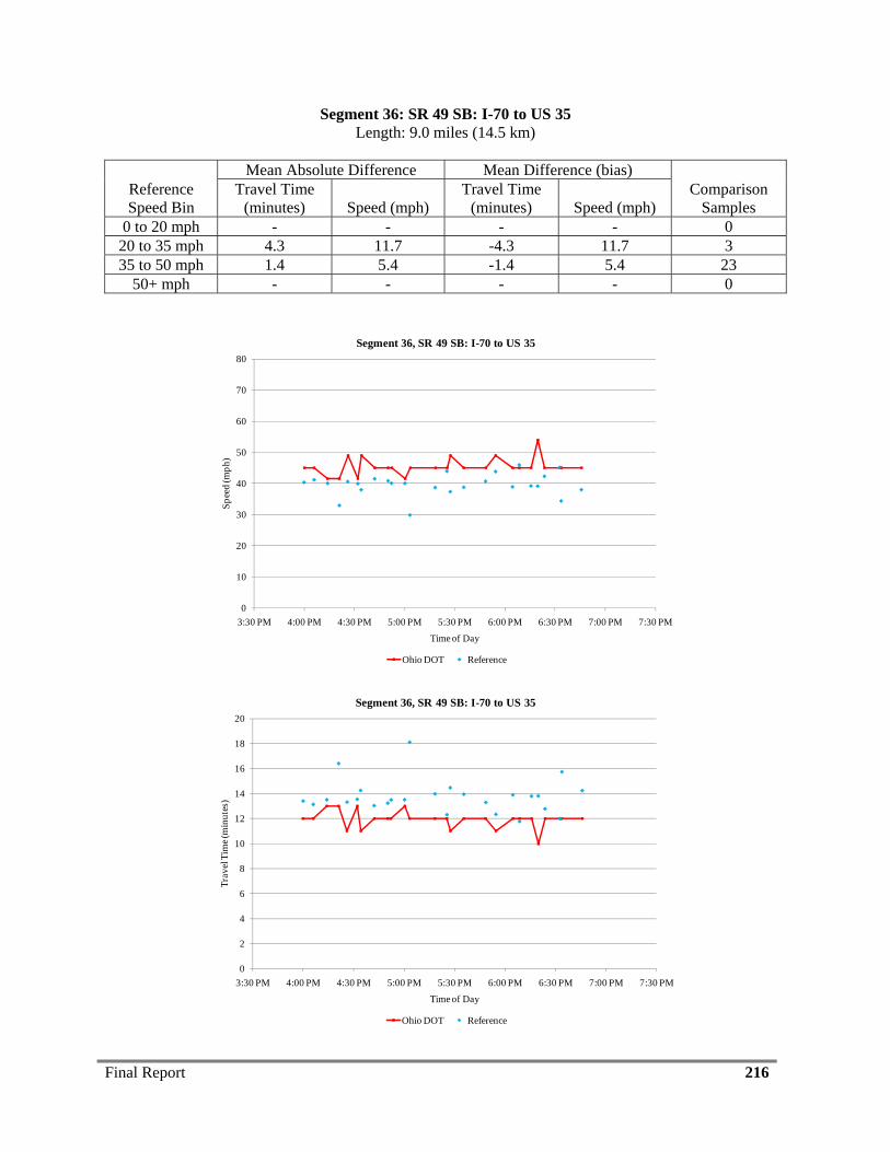
Final Report 216

Segment 36: SR 49 SB: I-70 to US 35 Length: 9.0 miles (14.5 km)

Reference Speed Bin


Samples Travel Time



20 to 35 mph 4.3 11.7 -4.3 11.7 3 35 to 50 mph 1.4 5.4 -1.4 5.4 23

50+ mph - - - - 0

0

10

20

30

40

50

60

70

80


Spee

d (m

ph)

Time of Day

Segment 36, SR 49 SB: I-70 to US 35

Ohio DOT Reference

0

2

4

6

8

10

12

14

16

18

20


Trav

el T

ime (

min

utes

)

Time of Day

Segment 36, SR 49 SB: I-70 to US 35

Ohio DOT Reference

Final Report 217

APPENDIX E

SPEED AND TRAVEL TIME DISTRIBUTION

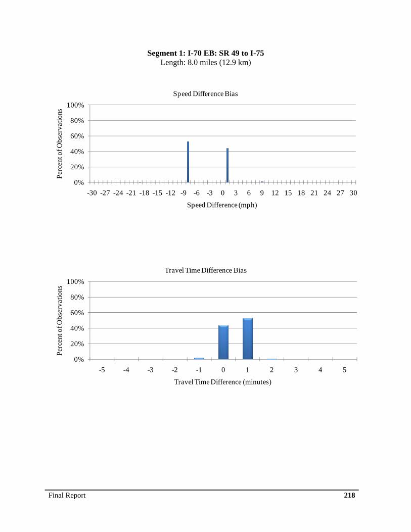
Final Report 218

Segment 1: I-70 EB: SR 49 to I-75 Length: 8.0 miles (12.9 km)

0%

20%

40%

60%

80%

100%

-30 -27 -24 -21 -18 -15 -12 -9 -6 -3 0 3 6 9 12 15 18 21 24 27 30

Perc

ent o

f Obs

erva

tions

Speed Difference (mph).

Speed Difference Bias

0%

20%

40%

60%

80%

100%

-5 -4 -3 -2 -1 0 1 2 3 4 5

Perc

ent o

f Obs

erva

tions

Travel Time Difference (minutes).

Travel Time Difference Bias

Final Report 219

0%

20%

40%

60%

80%

100%

0 3 6 9 12 15 18 21 24 27 30

Perc

ent o

f Obs

erva

tions


Absolute Speed Difference

0%

20%

40%

60%

80%

100%

0 1 2 3 4 5

Perc

ent o

f Obs

erva

tions


Absolute Travel Time Distance

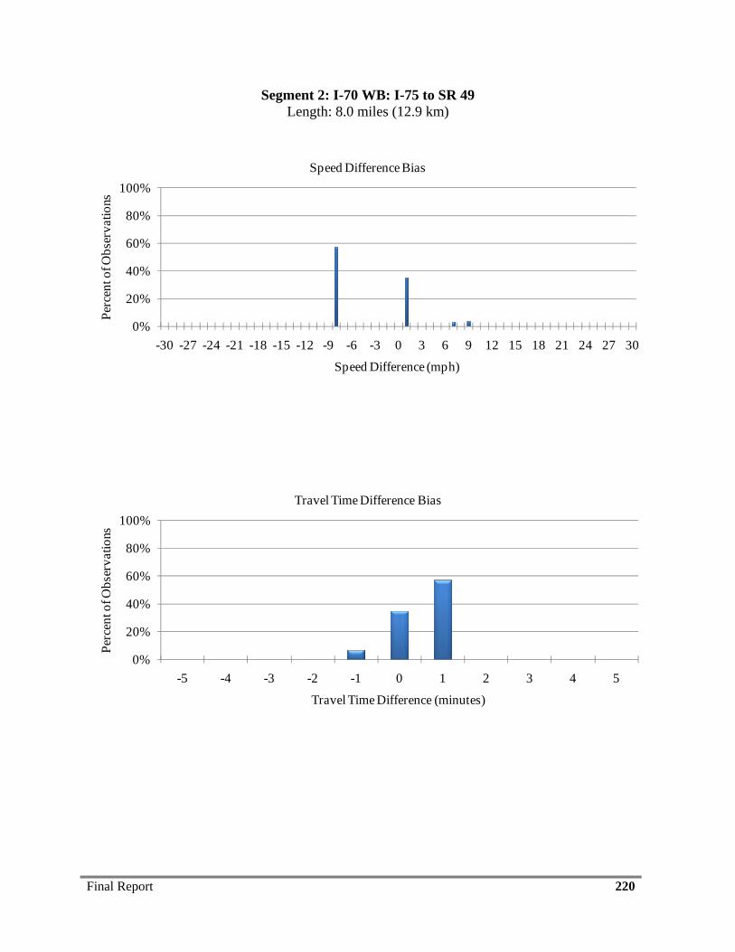
Final Report 220

Segment 2: I-70 WB: I-75 to SR 49 Length: 8.0 miles (12.9 km)

0%

20%

40%

60%

80%

100%

-30 -27 -24 -21 -18 -15 -12 -9 -6 -3 0 3 6 9 12 15 18 21 24 27 30

Perc

ent o

f Obs

erva

tions



0%

20%

40%

60%

80%

100%

-5 -4 -3 -2 -1 0 1 2 3 4 5

Perc

ent o

f Obs

erva

tions



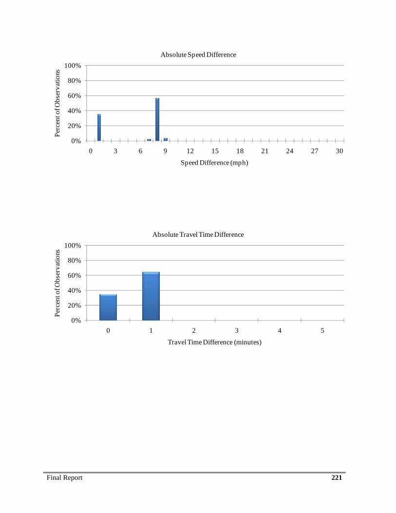
Final Report 221

0%

20%

40%

60%

80%

100%

0 3 6 9 12 15 18 21 24 27 30

Perc

ent o

f Obs

erva

tions



0%

20%

40%

60%

80%

100%

0 1 2 3 4 5

Perc

ent o

f Obs

erva

tions


Absolute Travel Time Difference

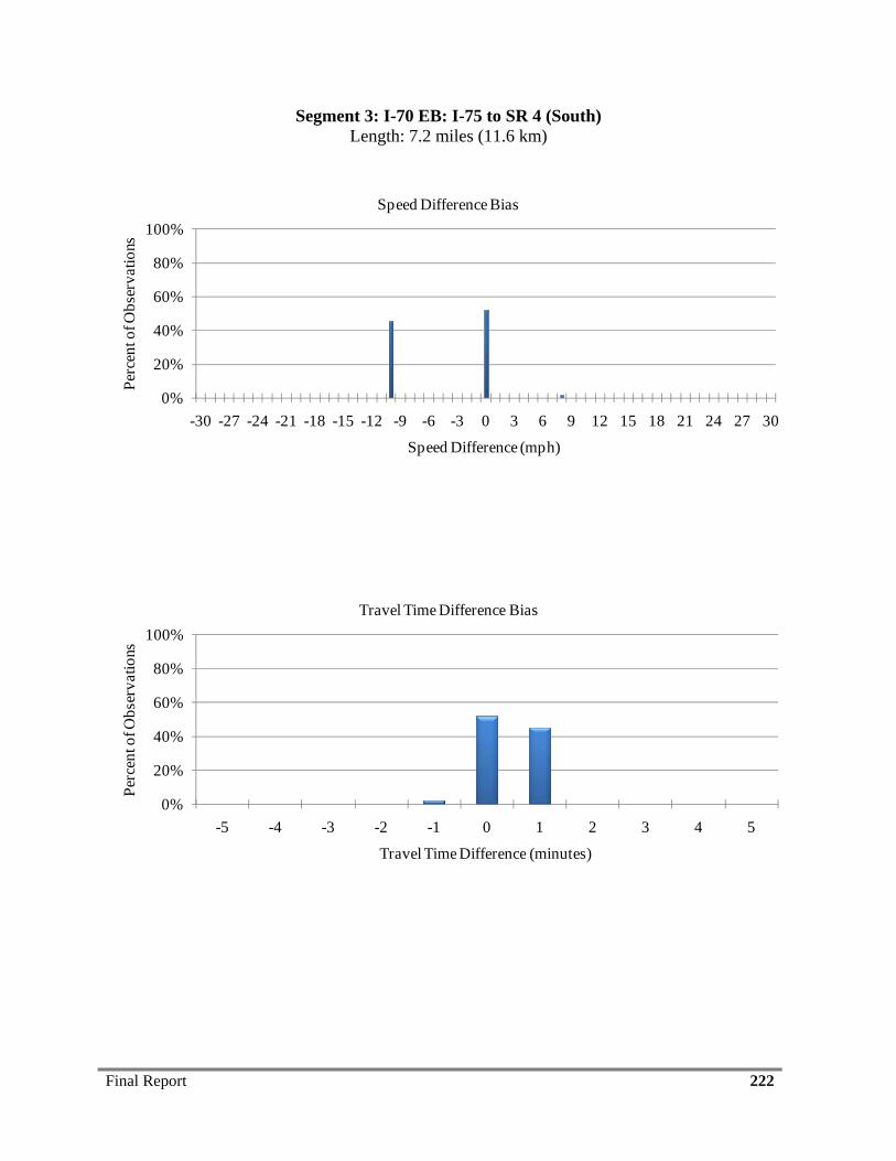
Final Report 222

Segment 3: I-70 EB: I-75 to SR 4 (South) Length: 7.2 miles (11.6 km)

0%

20%

40%

60%

80%

100%

-30 -27 -24 -21 -18 -15 -12 -9 -6 -3 0 3 6 9 12 15 18 21 24 27 30

Perc

ent o

f Obs

erva

tions



0%

20%

40%

60%

80%

100%

-5 -4 -3 -2 -1 0 1 2 3 4 5

Perc

ent o

f Obs

erva

tions



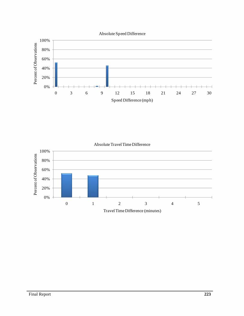
Final Report 223

0%

20%

40%

60%

80%

100%

0 3 6 9 12 15 18 21 24 27 30

Perc

ent o

f Obs

erva

tions



0%

20%

40%

60%

80%

100%

0 1 2 3 4 5

Perc

ent o

f Obs

erva

tions



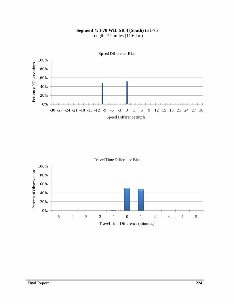
Final Report 224

Segment 4: I-70 WB: SR 4 (South) to I-75 Length: 7.2 miles (11.6 km)

0%

20%

40%

60%

80%

100%

-30 -27 -24 -21 -18 -15 -12 -9 -6 -3 0 3 6 9 12 15 18 21 24 27 30

Perc

ent o

f Obs

erva

tions



0%

20%

40%

60%

80%

100%

-5 -4 -3 -2 -1 0 1 2 3 4 5

Perc

ent o

f Obs

erva

tions



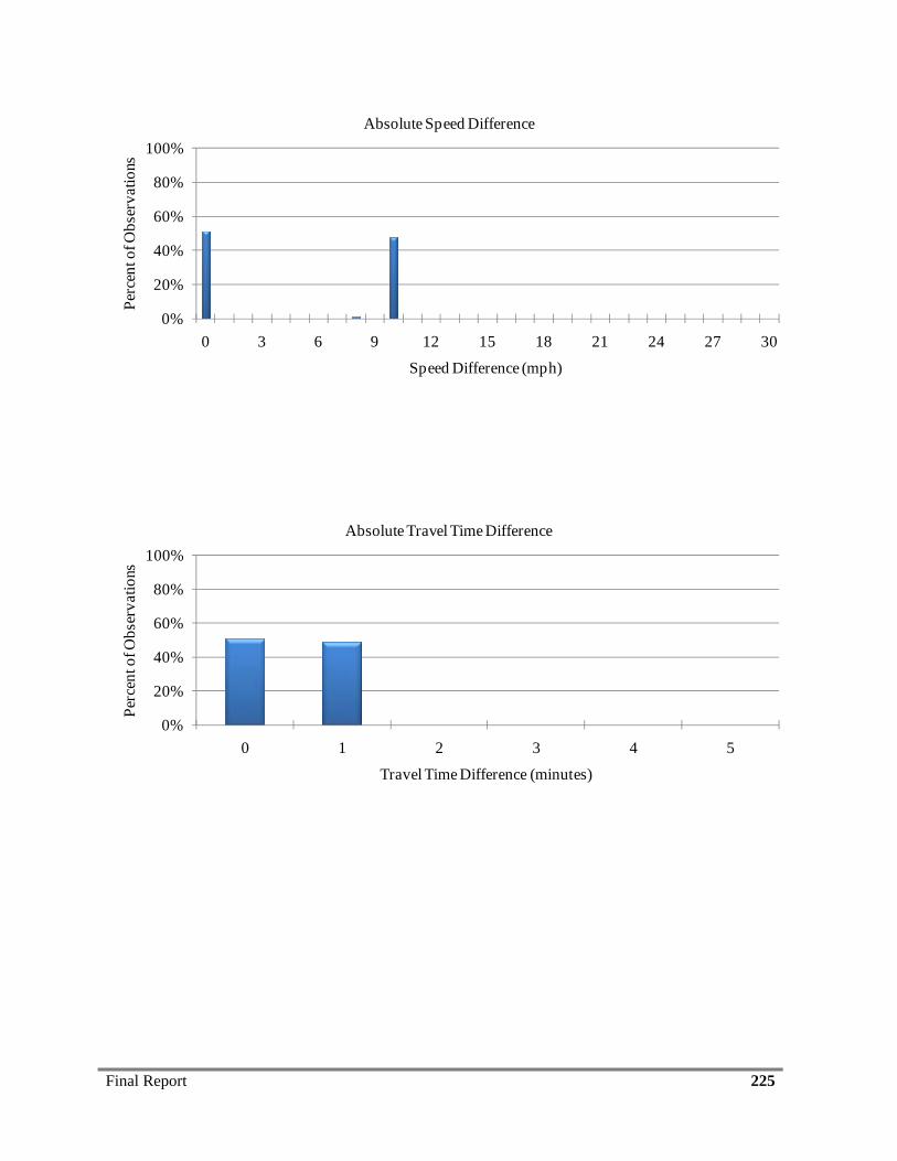
Final Report 225

0%

20%

40%

60%

80%

100%

0 3 6 9 12 15 18 21 24 27 30

Perc

ent o

f Obs

erva

tions



0%

20%

40%

60%

80%

100%

0 1 2 3 4 5

Perc

ent o

f Obs

erva

tions



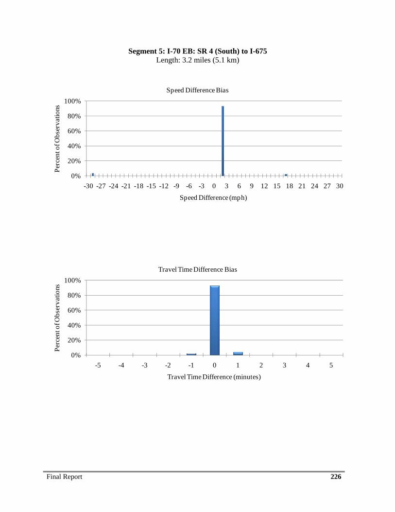
Final Report 226

Segment 5: I-70 EB: SR 4 (South) to I-675 Length: 3.2 miles (5.1 km)

0%

20%

40%

60%

80%

100%

-30 -27 -24 -21 -18 -15 -12 -9 -6 -3 0 3 6 9 12 15 18 21 24 27 30

Perc

ent o

f Obs

erva

tions



0%

20%

40%

60%

80%

100%

-5 -4 -3 -2 -1 0 1 2 3 4 5

Perc

ent o

f Obs

erva

tions



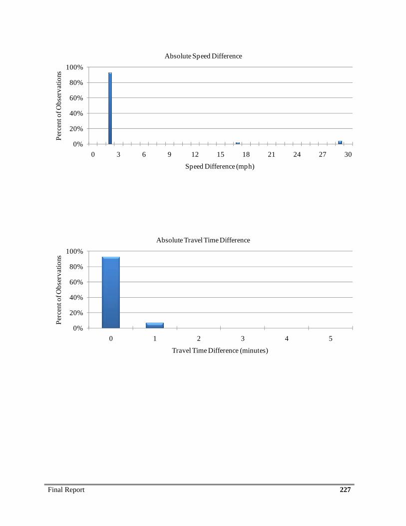
Final Report 227

0%

20%

40%

60%

80%

100%

0 3 6 9 12 15 18 21 24 27 30

Perc

ent o

f Obs

erva

tions



0%

20%

40%

60%

80%

100%

0 1 2 3 4 5

Perc

ent o

f Obs

erva

tions



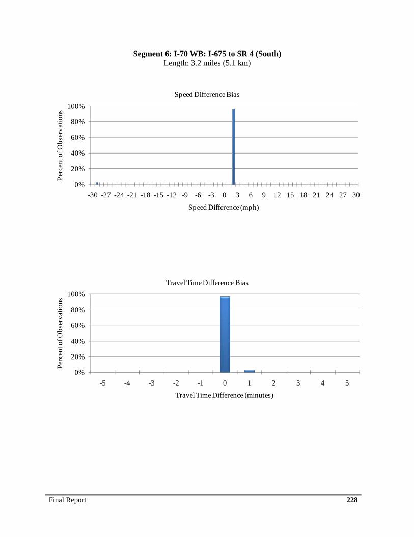
Final Report 228

Segment 6: I-70 WB: I-675 to SR 4 (South) Length: 3.2 miles (5.1 km)

0%

20%

40%

60%

80%

100%

-30 -27 -24 -21 -18 -15 -12 -9 -6 -3 0 3 6 9 12 15 18 21 24 27 30

Perc

ent o

f Obs

erva

tions



0%

20%

40%

60%

80%

100%

-5 -4 -3 -2 -1 0 1 2 3 4 5

Perc

ent o

f Obs

erva

tions



Final Report 229

0%

20%

40%

60%

80%

100%

0 3 6 9 12 15 18 21 24 27 30

Perc

ent o

f Obs

erva

tions



0%

20%

40%

60%

80%

100%

0 1 2 3 4 5

Perc

ent o

f Obs

erva

tions



Final Report 230

Segment 7: I-70 EB: I-675 to SR 4 (Enon) Length: 2.9 miles (4.7 km)


Final Report 231

Segment 8: I-70 WB: SR 4 (Enon) to I-675 Length: 2.9 miles (4.7 km)


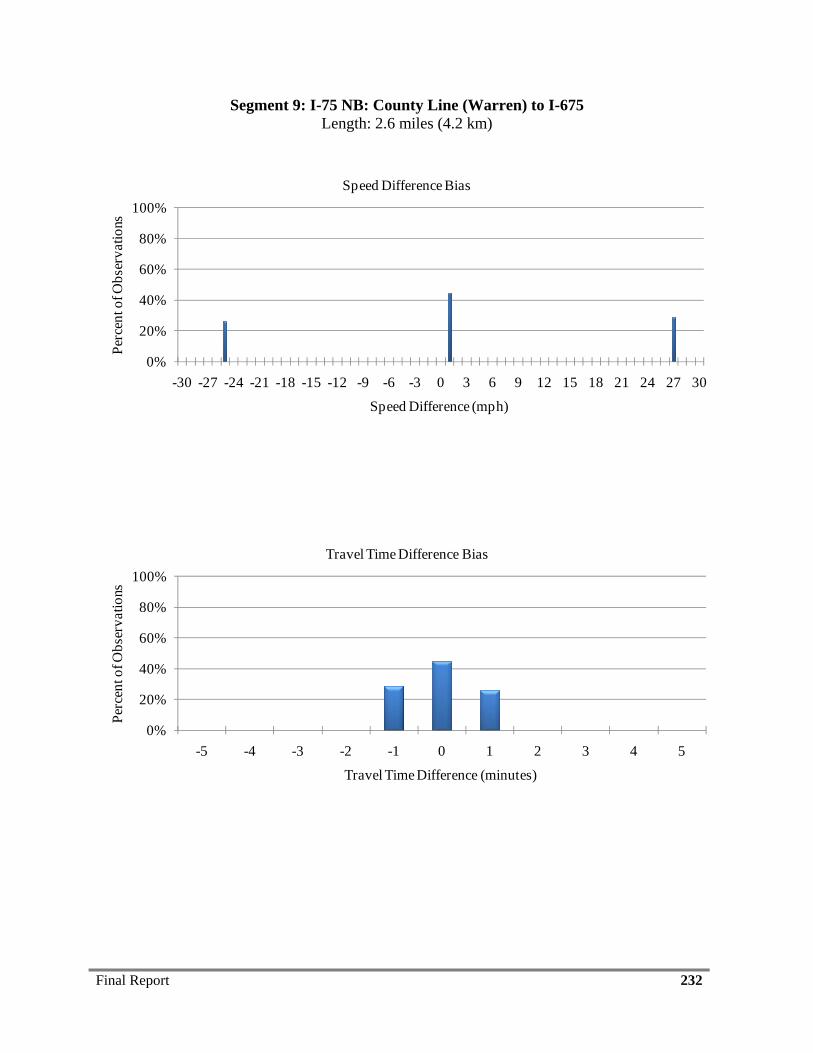
Final Report 232

Segment 9: I-75 NB: County Line (Warren) to I-675 Length: 2.6 miles (4.2 km)

0%

20%

40%

60%

80%

100%

-30 -27 -24 -21 -18 -15 -12 -9 -6 -3 0 3 6 9 12 15 18 21 24 27 30

Perc

ent o

f Obs

erva

tions



0%

20%

40%

60%

80%

100%

-5 -4 -3 -2 -1 0 1 2 3 4 5

Perc

ent o

f Obs

erva

tions



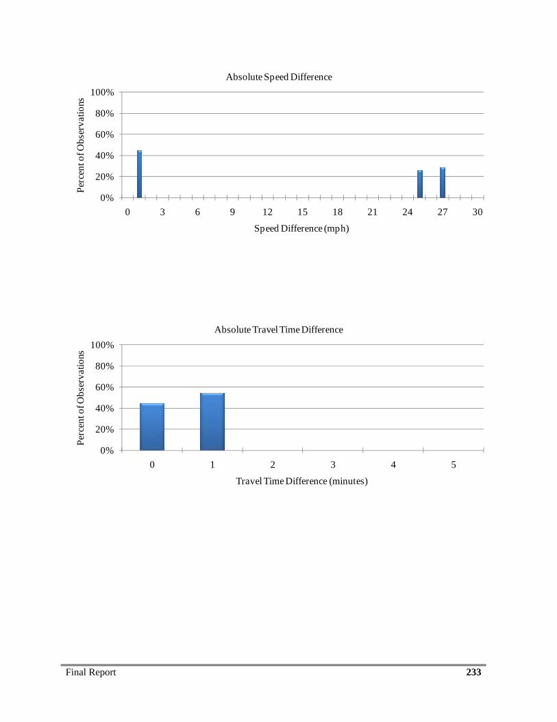
Final Report 233

0%

20%

40%

60%

80%

100%

0 3 6 9 12 15 18 21 24 27 30

Perc

ent o

f Obs

erva

tions



0%

20%

40%

60%

80%

100%

0 1 2 3 4 5

Perc

ent o

f Obs

erva

tions



Final Report 234

Segment 10: I-75 SB: I-675 to County Line (Warren) Length: 2.6 miles (4.2 km)

0%

20%

40%

60%

80%

100%

-30 -27 -24 -21 -18 -15 -12 -9 -6 -3 0 3 6 9 12 15 18 21 24 27 30

Perc

ent o

f Obs

erva

tions



0%

20%

40%

60%

80%

100%

-5 -4 -3 -2 -1 0 1 2 3 4 5

Perc

ent o

f Obs

erva

tions



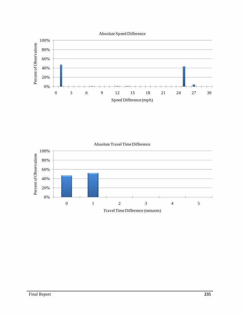
Final Report 235

0%

20%

40%

60%

80%

100%

0 3 6 9 12 15 18 21 24 27 30

Perc

ent o

f Obs

erva

tions



0%

20%

40%

60%

80%

100%

0 1 2 3 4 5

Perc

ent o

f Obs

erva

tions



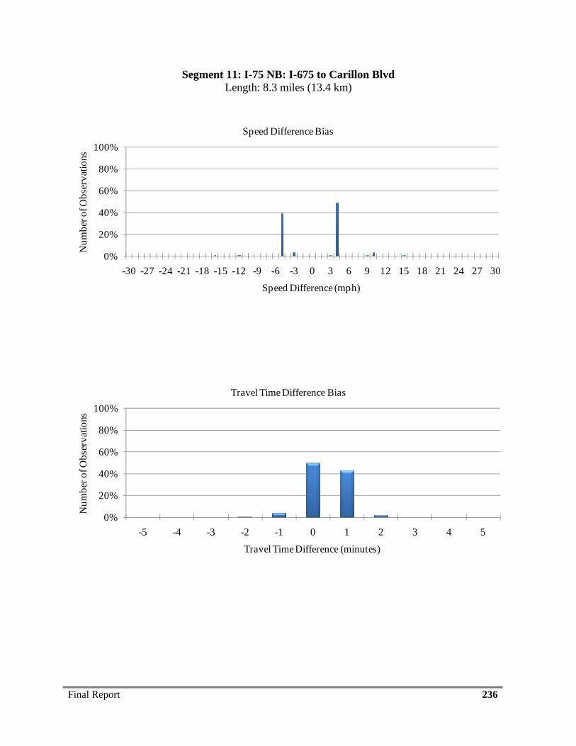
Final Report 236

Segment 11: I-75 NB: I-675 to Carillon Blvd Length: 8.3 miles (13.4 km)

0%

20%

40%

60%

80%

100%

-30 -27 -24 -21 -18 -15 -12 -9 -6 -3 0 3 6 9 12 15 18 21 24 27 30

Num

ber o

f Obs

erva

tions



0%

20%

40%

60%

80%

100%

-5 -4 -3 -2 -1 0 1 2 3 4 5

Num

ber o

f Obs

erva

tions



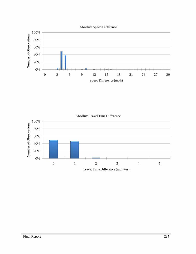
Final Report 237

0%

20%

40%

60%

80%

100%

0 3 6 9 12 15 18 21 24 27 30

Num

ber o

f Obs

erva

tions



0%

20%

40%

60%

80%

100%

0 1 2 3 4 5

Num

ber o

f Obs

erva

tions



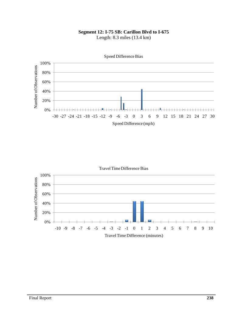
Final Report 238

Segment 12: I-75 SB: Carillon Blvd to I-675 Length: 8.3 miles (13.4 km)

0%

20%

40%

60%

80%

100%

-30 -27 -24 -21 -18 -15 -12 -9 -6 -3 0 3 6 9 12 15 18 21 24 27 30

Num

ber o

f Obs

erva

tions



0%

20%

40%

60%

80%

100%

-10 -9 -8 -7 -6 -5 -4 -3 -2 -1 0 1 2 3 4 5 6 7 8 9 10

Num

ber o

f Obs

erva

tions



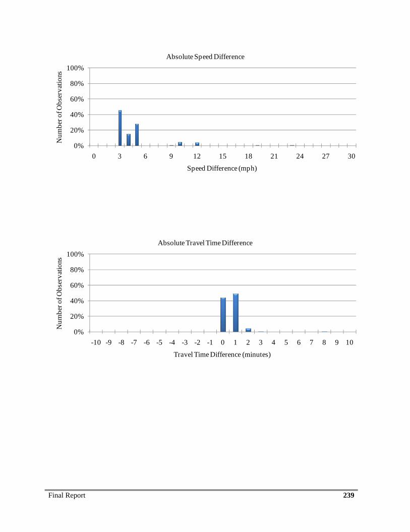
Final Report 239

0%

20%

40%

60%

80%

100%

0 3 6 9 12 15 18 21 24 27 30

Num

ber o

f Obs

erva

tions



0%

20%

40%

60%

80%

100%

-10 -9 -8 -7 -6 -5 -4 -3 -2 -1 0 1 2 3 4 5 6 7 8 9 10

Num

ber o

f Obs

erva

tions



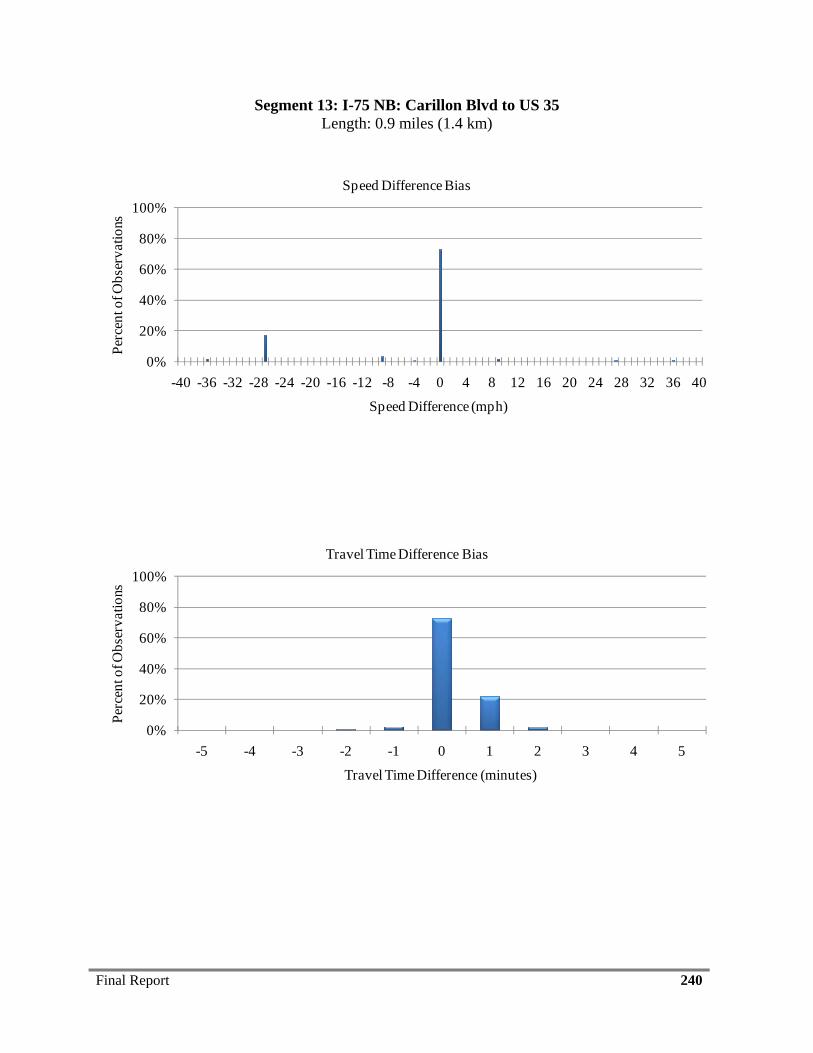
Final Report 240

Segment 13: I-75 NB: Carillon Blvd to US 35 Length: 0.9 miles (1.4 km)

0%

20%

40%

60%

80%

100%

-40 -36 -32 -28 -24 -20 -16 -12 -8 -4 0 4 8 12 16 20 24 28 32 36 40

Perc

ent o

f Obs

erva

tions



0%

20%

40%

60%

80%

100%

-5 -4 -3 -2 -1 0 1 2 3 4 5

Perc

ent o

f Obs

erva

tions



Final Report 241

0%

20%

40%

60%

80%

100%

0 4 8 12 16 20 24 28 32 36 40

Perc

ent o

f Obs

erva

tions



0%

20%

40%

60%

80%

100%

0 1 2 3 4 5

Perc

ent o

f Obs

erva

tions



Final Report 242

Segment 14: I-75 SB: US 35 to Carillon Blvd Length: 0.9 miles (1.4 km)

0%

20%

40%

60%

80%

100%

-30 -27 -24 -21 -18 -15 -12 -9 -6 -3 0 3 6 9 12 15 18 21 24 27 30

Perc

ent o

f Obs

erva

tions



0%

20%

40%

60%

80%

100%

-5 -4 -3 -2 -1 0 1 2 3 4 5

Perc

ent o

f Obs

erva

tions



Final Report 243

0%

20%

40%

60%

80%

100%

0 3 6 9 12 15 18 21 24 27 30

Perc

ent o

f Obs

erva

tions



0%

20%

40%

60%

80%

100%

0 1 2 3 4 5

Perc

ent o

f Obs

erva

tions



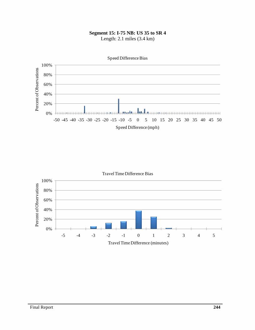
Final Report 244

Segment 15: I-75 NB: US 35 to SR 4 Length: 2.1 miles (3.4 km)

0%

20%

40%

60%

80%

100%

-50 -45 -40 -35 -30 -25 -20 -15 -10 -5 0 5 10 15 20 25 30 35 40 45 50

Perc

ent o

f Obs

erva

tions



0%

20%

40%

60%

80%

100%

-5 -4 -3 -2 -1 0 1 2 3 4 5

Perc

ent o

f Obs

erva

tions



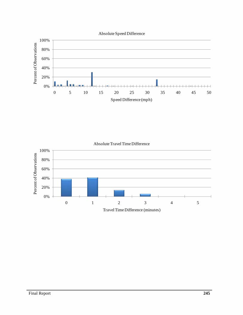
Final Report 245

0%

20%

40%

60%

80%

100%

0 5 10 15 20 25 30 35 40 45 50

Perc

ent o

f Obs

erva

tions



0%

20%

40%

60%

80%

100%

0 1 2 3 4 5

Perc

ent o

f Obs

erva

tions



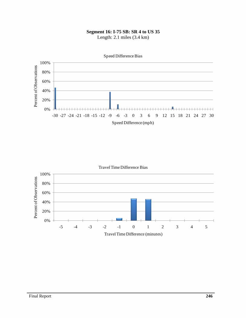
Final Report 246

Segment 16: I-75 SB: SR 4 to US 35 Length: 2.1 miles (3.4 km)

0%

20%

40%

60%

80%

100%

-30 -27 -24 -21 -18 -15 -12 -9 -6 -3 0 3 6 9 12 15 18 21 24 27 30

Perc

ent o

f Obs

erva

tions



0%

20%

40%

60%

80%

100%

-5 -4 -3 -2 -1 0 1 2 3 4 5

Perc

ent o

f Obs

erva

tions



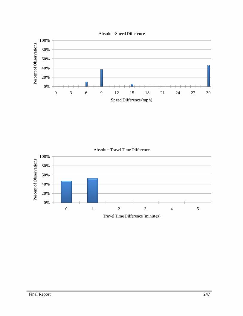
Final Report 247

0%

20%

40%

60%

80%

100%

0 3 6 9 12 15 18 21 24 27 30

Perc

ent o

f Obs

erva

tions



0%

20%

40%

60%

80%

100%

0 1 2 3 4 5

Perc

ent o

f Obs

erva

tions



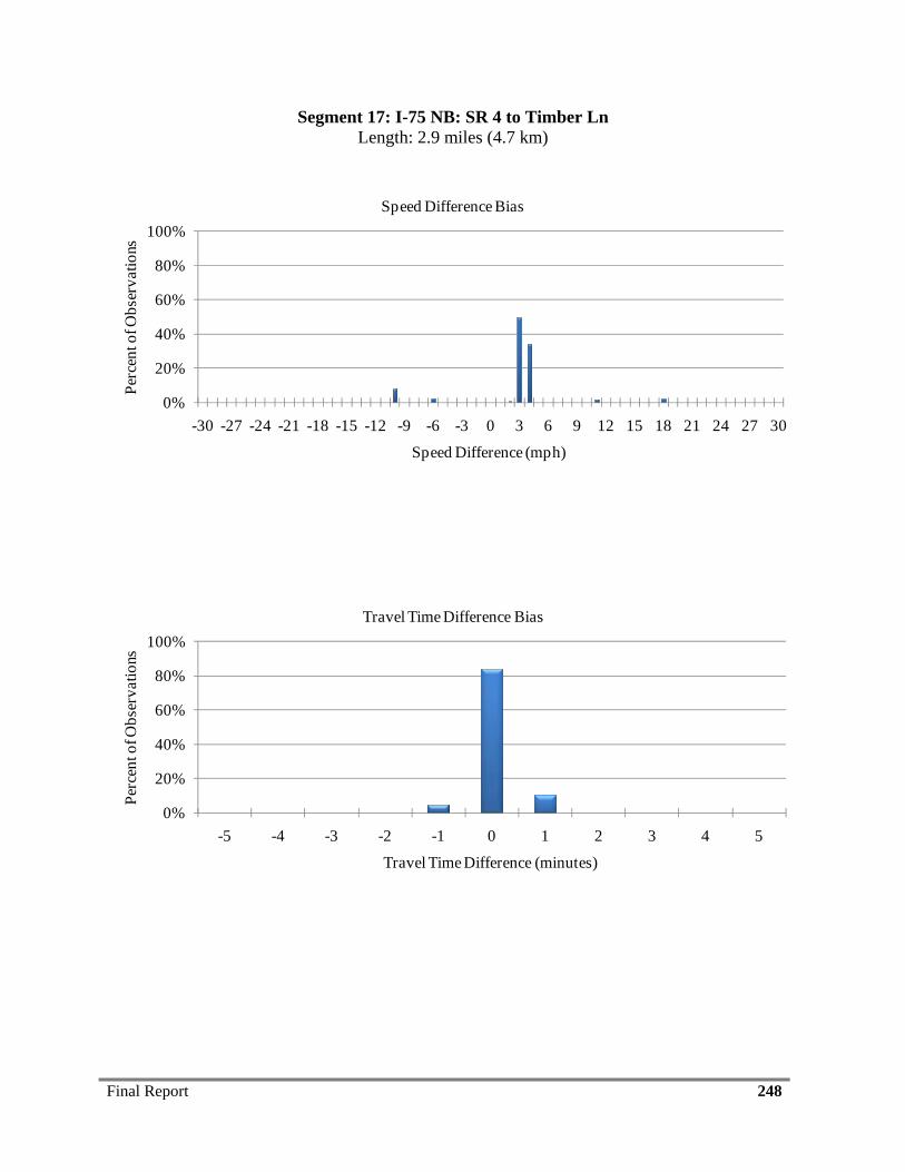
Final Report 248

Segment 17: I-75 NB: SR 4 to Timber Ln Length: 2.9 miles (4.7 km)

0%

20%

40%

60%

80%

100%

-30 -27 -24 -21 -18 -15 -12 -9 -6 -3 0 3 6 9 12 15 18 21 24 27 30

Perc

ent o

f Obs

erva

tions



0%

20%

40%

60%

80%

100%

-5 -4 -3 -2 -1 0 1 2 3 4 5

Perc

ent o

f Obs

erva

tions



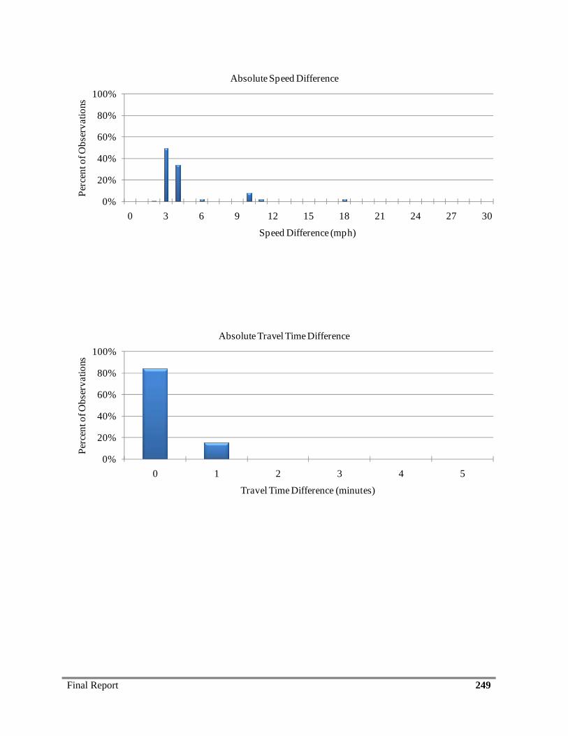
Final Report 249

0%

20%

40%

60%

80%

100%

0 3 6 9 12 15 18 21 24 27 30

Perc

ent o

f Obs

erva

tions



0%

20%

40%

60%

80%

100%

0 1 2 3 4 5

Perc

ent o

f Obs

erva

tions



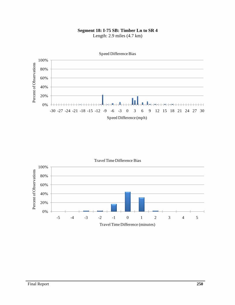
Final Report 250

Segment 18: I-75 SB: Timber Ln to SR 4 Length: 2.9 miles (4.7 km)

0%

20%

40%

60%

80%

100%

-30 -27 -24 -21 -18 -15 -12 -9 -6 -3 0 3 6 9 12 15 18 21 24 27 30

Perc

ent o

f Obs

erva

tions



0%

20%

40%

60%

80%

100%

-5 -4 -3 -2 -1 0 1 2 3 4 5

Perc

ent o

f Obs

erva

tions



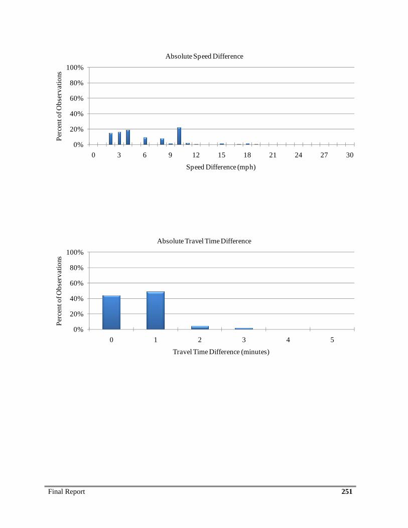
Final Report 251

0%

20%

40%

60%

80%

100%

0 3 6 9 12 15 18 21 24 27 30

Perc

ent o

f Obs

erva

tions



0%

20%

40%

60%

80%

100%

0 1 2 3 4 5

Perc

ent o

f Obs

erva

tions



Final Report 252

Segment 19: I-75 NB: Timber Ln to I-70 Length: 3.7 miles (6.0 km)

0%

20%

40%

60%

80%

100%

-30 -27 -24 -21 -18 -15 -12 -9 -6 -3 0 3 6 9 12 15 18 21 24 27 30

Perc

ent o

f Obs

erva

tions



0%

20%

40%

60%

80%

100%

-5 -4 -3 -2 -1 0 1 2 3 4 5

Perc

ent o

f Obs

erva

tions



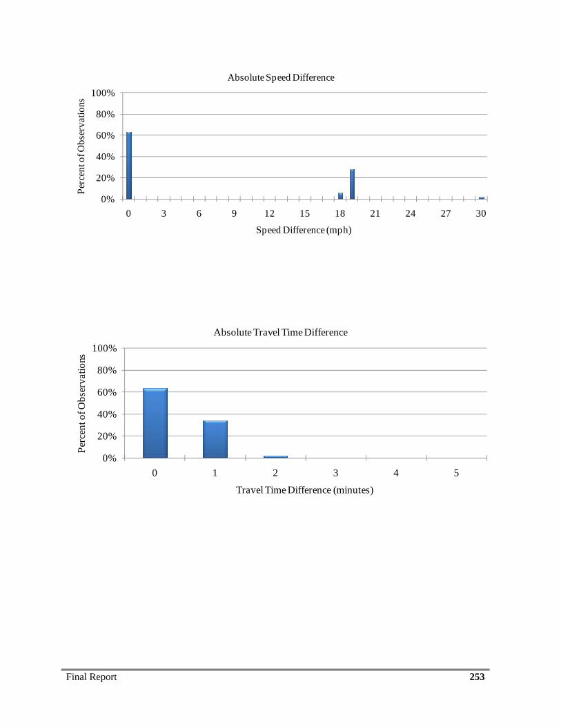
Final Report 253

0%

20%

40%

60%

80%

100%

0 3 6 9 12 15 18 21 24 27 30

Perc

ent o

f Obs

erva

tions



0%

20%

40%

60%

80%

100%

0 1 2 3 4 5

Perc

ent o

f Obs

erva

tions



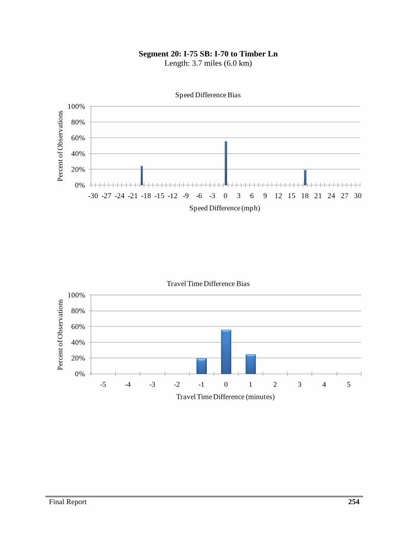
Final Report 254

Segment 20: I-75 SB: I-70 to Timber Ln Length: 3.7 miles (6.0 km)

0%

20%

40%

60%

80%

100%

-30 -27 -24 -21 -18 -15 -12 -9 -6 -3 0 3 6 9 12 15 18 21 24 27 30

Perc

ent o

f Obs

erva

tions



0%

20%

40%

60%

80%

100%

-5 -4 -3 -2 -1 0 1 2 3 4 5

Perc

ent o

f Obs

erva

tions



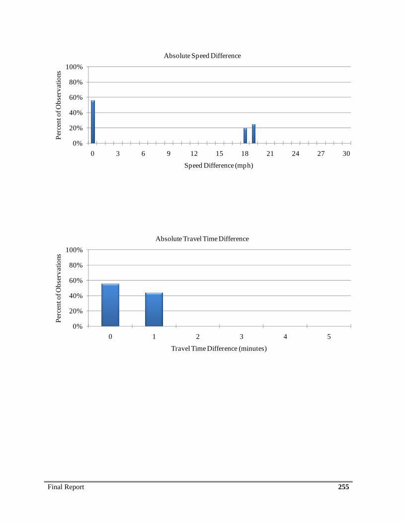
Final Report 255

0%

20%

40%

60%

80%

100%

0 3 6 9 12 15 18 21 24 27 30

Perc

ent o

f Obs

erva

tions



0%

20%

40%

60%

80%

100%

0 1 2 3 4 5

Perc

ent o

f Obs

erva

tions



Final Report 256


0%

20%

40%

60%

80%

100%

-50 -45 -40 -35 -30 -25 -20 -15 -10 -5 0 5 10 15 20 25 30 35 40 45 50

Perc

ent o

f Obs

erva

tions



0%

20%

40%

60%

80%

100%

-5 -4 -3 -2 -1 0 1 2 3 4 5

Perc

ent o

f Obs

erva

tions



Final Report 257

0%

20%

40%

60%

80%

100%

0 5 10 15 20 25 30 35 40 45 50

Perc

ent o

f Obs

erva

tions



0%

20%

40%

60%

80%

100%

0 1 2 3 4 5

Perc

ent o

f Obs

erva

tion



Final Report 258


0%

20%

40%

60%

80%

100%

-50 -45 -40 -35 -30 -25 -20 -15 -10 -5 0 5 10 15 20 25 30 35 40 45 50

Perc

ent o

f Obs

erva

tions



0%

20%

40%

60%

80%

100%

-5 -4 -3 -2 -1 0 1 2 3 4 5

Perc

ent o

f Obs

erva

tions



Final Report 259

0%

20%

40%

60%

80%

100%

0 5 10 15 20 25 30 35 40 45 50

Perc

ent o

f Obs

erva

tions



0%

20%

40%

60%

80%

100%

0 1 2 3 4 5

Perc

ent o

f Obs

erva

tions



Final Report 260

Segment 23: I-75 NB: US 40 to County Line (Miami) Length: 2.1 miles (3.4 km)

0%

20%

40%

60%

80%

100%

-30 -27 -24 -21 -18 -15 -12 -9 -6 -3 0 3 6 9 12 15 18 21 24 27 30

Perc

ent o

f Obs

erva

tions



0%

20%

40%

60%

80%

100%

-5 -4 -3 -2 -1 0 1 2 3 4 5

Perc

ent o

f Obs

erva

tions



Final Report 261

0%

20%

40%

60%

80%

100%

0 3 6 9 12 15 18 21 24 27 30

Perc

ent o

f Obs

erva

tions



0%

20%

40%

60%

80%

100%

0 1 2 3 4 5

Perc

ent o

f Obs

erva

tions



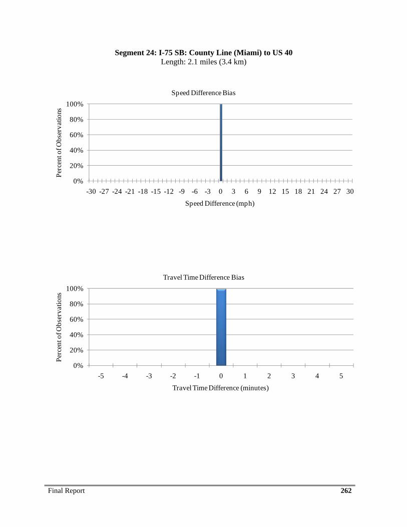
Final Report 262

Segment 24: I-75 SB: County Line (Miami) to US 40 Length: 2.1 miles (3.4 km)

0%

20%

40%

60%

80%

100%

-30 -27 -24 -21 -18 -15 -12 -9 -6 -3 0 3 6 9 12 15 18 21 24 27 30

Perc

ent o

f Obs

erva

tions



0%

20%

40%

60%

80%

100%

-5 -4 -3 -2 -1 0 1 2 3 4 5

Perc

ent o

f Obs

erva

tions



Final Report 263

0%

20%

40%

60%

80%

100%

0 3 6 9 12 15 18 21 24 27 30

Perc

ent o

f Obs

erva

tions



0%

20%

40%

60%

80%

100%

0 1 2 3 4 5

Perc

ent o

f Obs

erva

tions



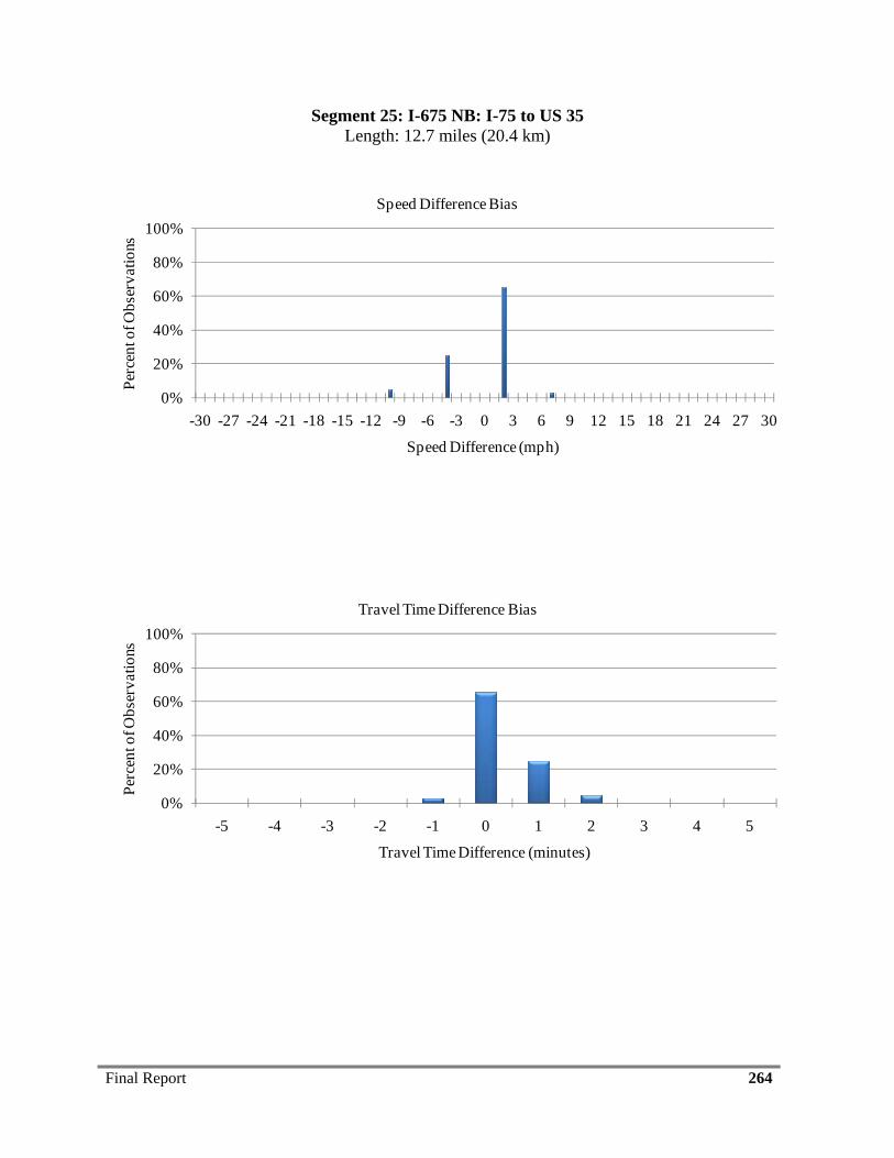
Final Report 264


0%

20%

40%

60%

80%

100%

-30 -27 -24 -21 -18 -15 -12 -9 -6 -3 0 3 6 9 12 15 18 21 24 27 30

Perc

ent o

f Obs

erva

tions



0%

20%

40%

60%

80%

100%

-5 -4 -3 -2 -1 0 1 2 3 4 5

Perc

ent o

f Obs

erva

tions



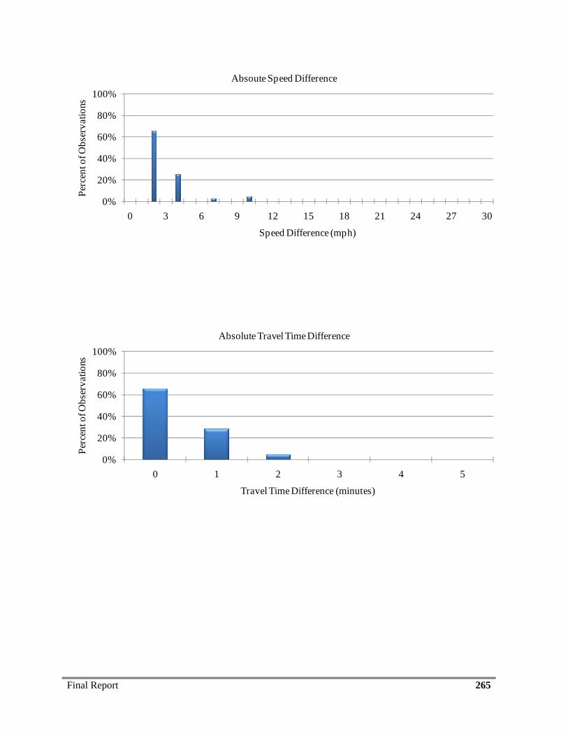
Final Report 265

0%

20%

40%

60%

80%

100%

0 3 6 9 12 15 18 21 24 27 30

Perc

ent o

f Obs

erva

tions


Absoute Speed Difference

0%

20%

40%

60%

80%

100%

0 1 2 3 4 5

Perc

ent o

f Obs

erva

tions



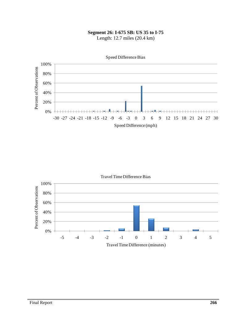
Final Report 266


0%

20%

40%

60%

80%

100%

-30 -27 -24 -21 -18 -15 -12 -9 -6 -3 0 3 6 9 12 15 18 21 24 27 30

Perc

ent o

f Obs

erva

tions



0%

20%

40%

60%

80%

100%

-5 -4 -3 -2 -1 0 1 2 3 4 5

Perc

ent o

f Obs

erva

tions



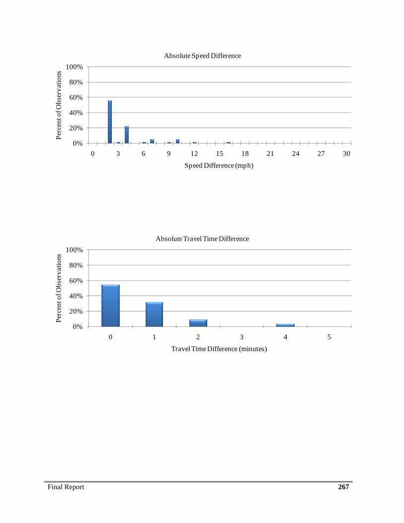
Final Report 267

0%

20%

40%

60%

80%

100%

0 3 6 9 12 15 18 21 24 27 30

Perc

ent o

f Obs

erva

tions



0%

20%

40%

60%

80%

100%

0 1 2 3 4 5

Perc

ent o

f Obs

erva

tions



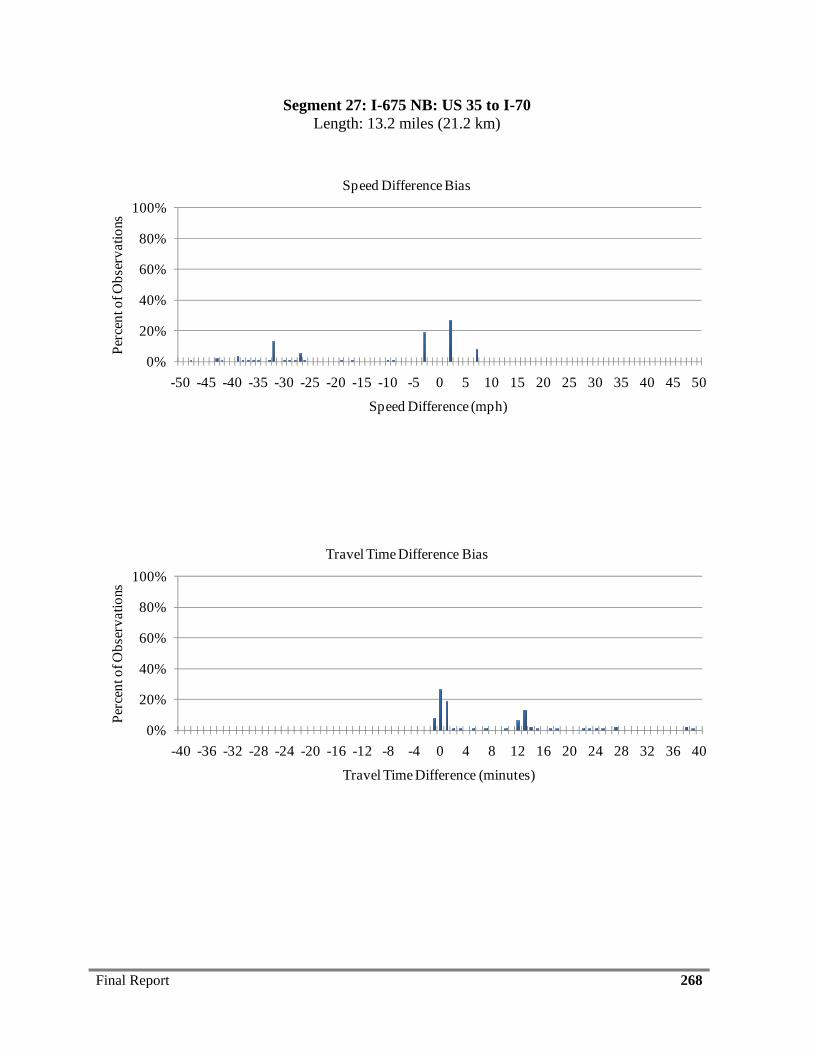
Final Report 268

Segment 27: I-675 NB: US 35 to I-70 Length: 13.2 miles (21.2 km)

0%

20%

40%

60%

80%

100%

-50 -45 -40 -35 -30 -25 -20 -15 -10 -5 0 5 10 15 20 25 30 35 40 45 50

Perc

ent o

f Obs

erva

tions



0%

20%

40%

60%

80%

100%

-40 -36 -32 -28 -24 -20 -16 -12 -8 -4 0 4 8 12 16 20 24 28 32 36 40

Perc

ent o

f Obs

erva

tions



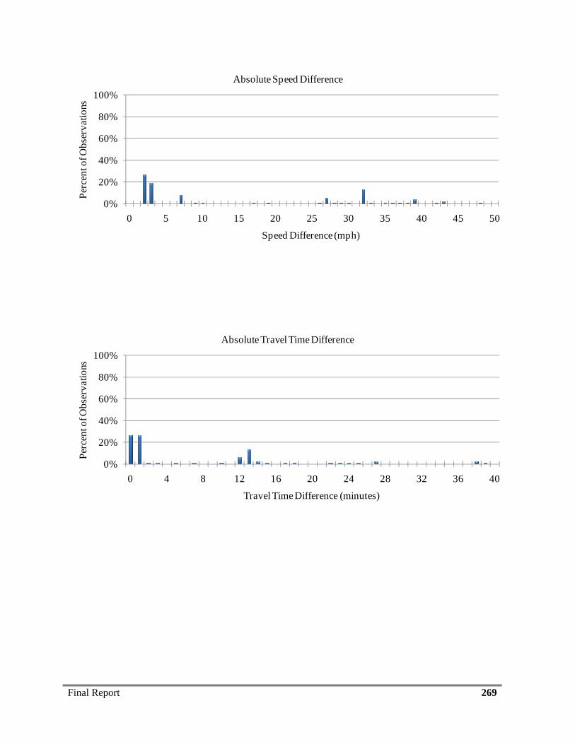
Final Report 269

0%

20%

40%

60%

80%

100%

0 5 10 15 20 25 30 35 40 45 50

Perc

ent o

f Obs

erva

tions



0%

20%

40%

60%

80%

100%

0 4 8 12 16 20 24 28 32 36 40

Perc

ent o

f Obs

erva

tions



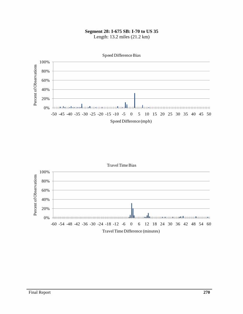
Final Report 270

Segment 28: I-675 SB: I-70 to US 35 Length: 13.2 miles (21.2 km)

0%

20%

40%

60%

80%

100%

-50 -45 -40 -35 -30 -25 -20 -15 -10 -5 0 5 10 15 20 25 30 35 40 45 50

Perc

ent o

f Obs

erva

tions



0%

20%

40%

60%

80%

100%

-60 -54 -48 -42 -36 -30 -24 -18 -12 -6 0 6 12 18 24 30 36 42 48 54 60

Perc

ent o

f Obs

erva

tions


Travel Time Bias

Final Report 271

0%

20%

40%

60%

80%

100%

0 5 10 15 20 25 30 35 40 45 50

Perc

ent o

f Obs

erva

tions



0%

20%

40%

60%

80%

100%

0 6 12 18 24 30 36 42 48 54 60

Perc

ent o

f Obs

erva

tions



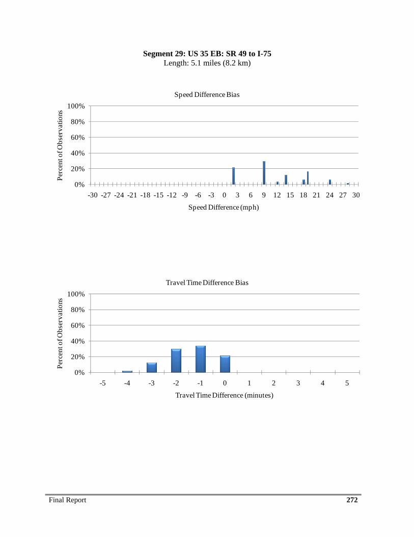
Final Report 272

Segment 29: US 35 EB: SR 49 to I-75 Length: 5.1 miles (8.2 km)

0%

20%

40%

60%

80%

100%

-30 -27 -24 -21 -18 -15 -12 -9 -6 -3 0 3 6 9 12 15 18 21 24 27 30

Perc

ent o

f Obs

erva

tions



0%

20%

40%

60%

80%

100%

-5 -4 -3 -2 -1 0 1 2 3 4 5

Perc

ent o

f Obs

erva

tions



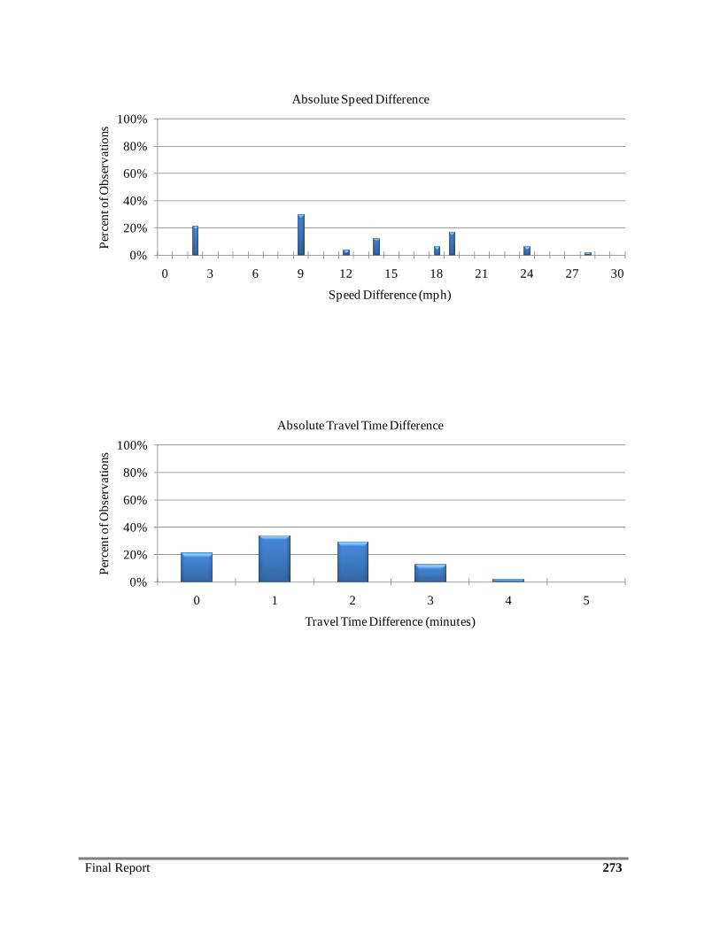
Final Report 273

0%

20%

40%

60%

80%

100%

0 3 6 9 12 15 18 21 24 27 30

Perc

ent o

f Obs

erva

tions



0%

20%

40%

60%

80%

100%

0 1 2 3 4 5

Perc

ent o

f Obs

erva

tions



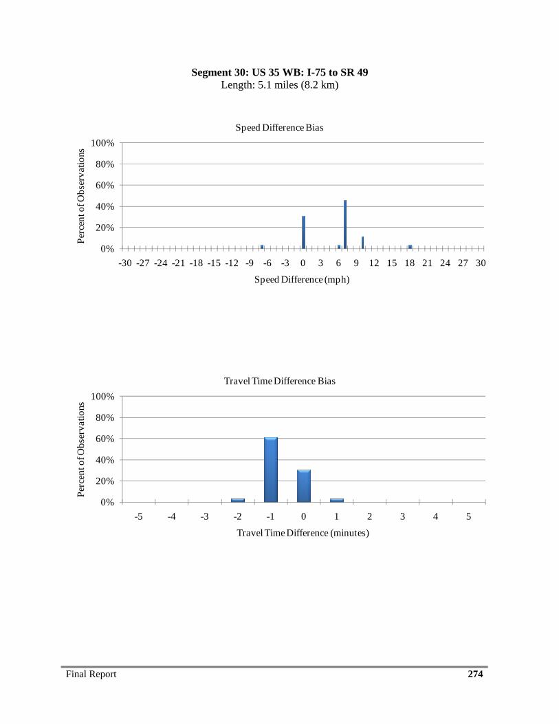
Final Report 274

Segment 30: US 35 WB: I-75 to SR 49 Length: 5.1 miles (8.2 km)

0%

20%

40%

60%

80%

100%

-30 -27 -24 -21 -18 -15 -12 -9 -6 -3 0 3 6 9 12 15 18 21 24 27 30

Perc

ent o

f Obs

erva

tions



0%

20%

40%

60%

80%

100%

-5 -4 -3 -2 -1 0 1 2 3 4 5

Perc

ent o

f Obs

erva

tions



Final Report 275

0%

20%

40%

60%

80%

100%

0 3 6 9 12 15 18 21 24 27 30

Perc

ent o

f Obs

erva

tions



0%

20%

40%

60%

80%

100%

0 1 2 3 4 5

Perc

ent o

f Obs

erva

tions



Final Report 276

Segment 31: US 35 EB: I-75 to I-675 Length: 6.4 miles (10.3 km)

0%

20%

40%

60%

80%

100%

-30 -27 -24 -21 -18 -15 -12 -9 -6 -3 0 3 6 9 12 15 18 21 24 27 30

Perc

ent o

f Obs

erva

tions



0%

20%

40%

60%

80%

100%

-5 -4 -3 -2 -1 0 1 2 3 4 5

Perc

ent o

f Obs

erva

tions



Final Report 277

0%

20%

40%

60%

80%

100%

0 3 6 9 12 15 18 21 24 27 30

Perc

ent o

f Obs

erva

tions



0%

20%

40%

60%

80%

100%

0 1 2 3 4 5

Perc

ent o

f Obs

erva

tion



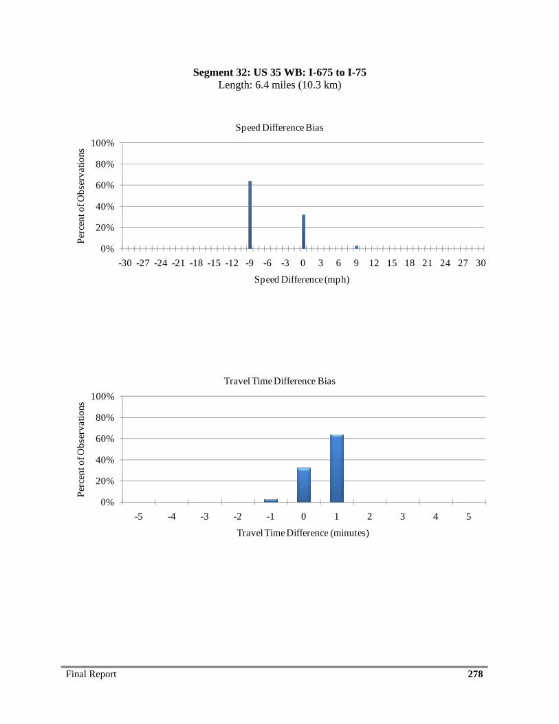
Final Report 278

Segment 32: US 35 WB: I-675 to I-75 Length: 6.4 miles (10.3 km)

0%

20%

40%

60%

80%

100%

-30 -27 -24 -21 -18 -15 -12 -9 -6 -3 0 3 6 9 12 15 18 21 24 27 30

Perc

ent o

f Obs

erva

tions



0%

20%

40%

60%

80%

100%

-5 -4 -3 -2 -1 0 1 2 3 4 5

Perc

ent o

f Obs

erva

tions



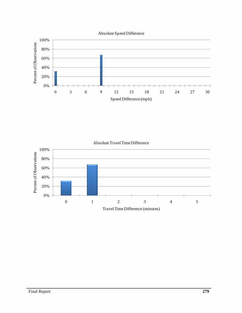
Final Report 279

0%

20%

40%

60%

80%

100%

0 3 6 9 12 15 18 21 24 27 30

Perc

ent o

f Obs

erva

tions



0%

20%

40%

60%

80%

100%

0 1 2 3 4 5

Perc

ent o

f Obs

erva

tions



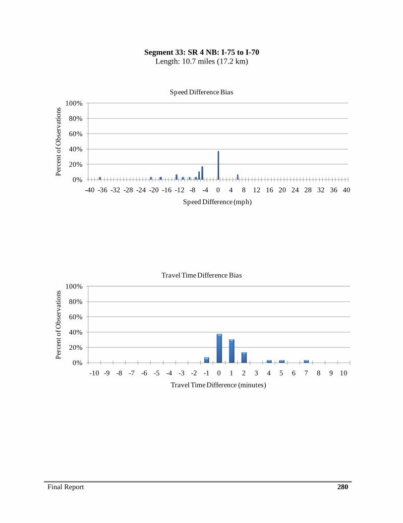
Final Report 280

Segment 33: SR 4 NB: I-75 to I-70 Length: 10.7 miles (17.2 km)

0%

20%

40%

60%

80%

100%

-40 -36 -32 -28 -24 -20 -16 -12 -8 -4 0 4 8 12 16 20 24 28 32 36 40

Perc

ent o

f Obs

erva

tions



0%

20%

40%

60%

80%

100%

-10 -9 -8 -7 -6 -5 -4 -3 -2 -1 0 1 2 3 4 5 6 7 8 9 10

Perc

ent o

f Obs

erva

tions



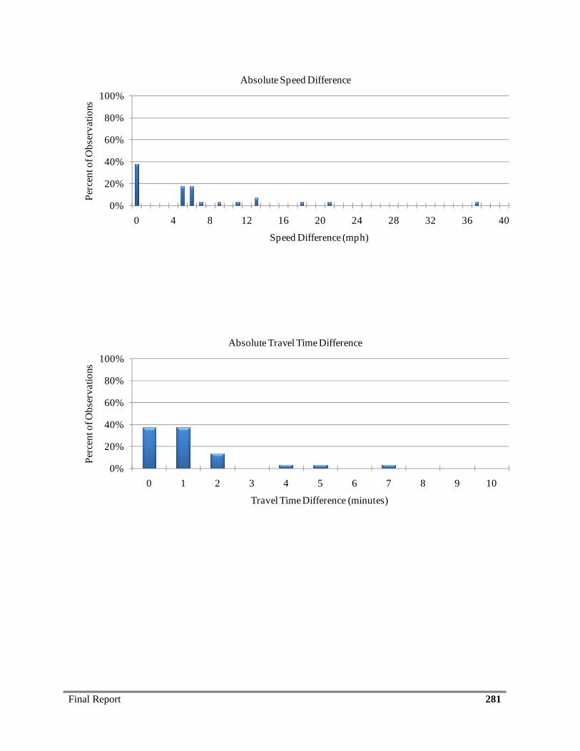
Final Report 281

0%

20%

40%

60%

80%

100%

0 4 8 12 16 20 24 28 32 36 40

Perc

ent o

f Obs

erva

tions



0%

20%

40%

60%

80%

100%

0 1 2 3 4 5 6 7 8 9 10

Perc

ent o

f Obs

erva

tions



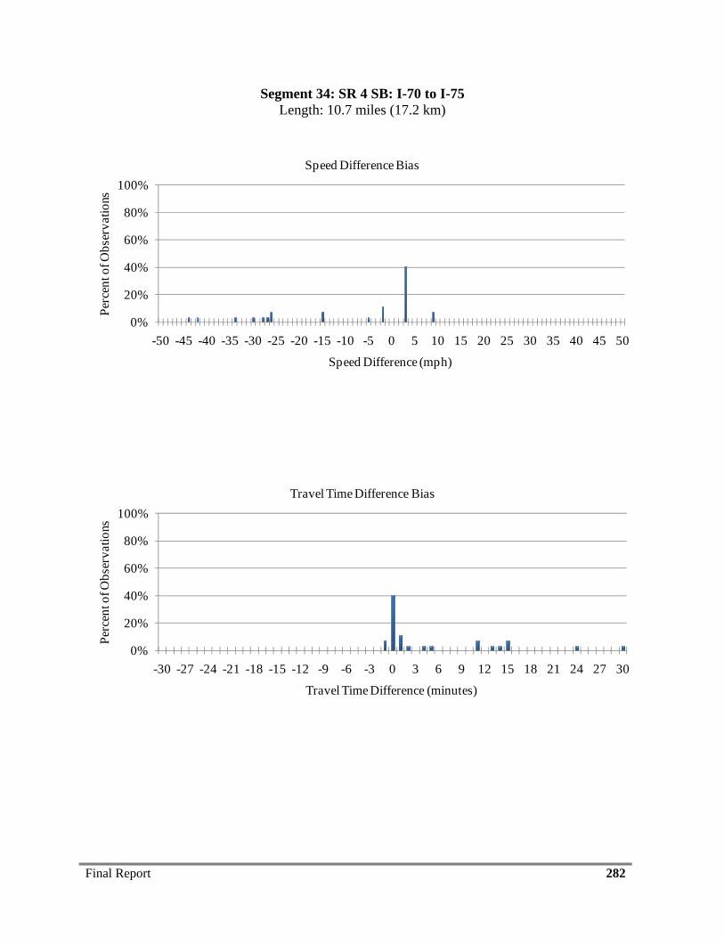
Final Report 282

Segment 34: SR 4 SB: I-70 to I-75 Length: 10.7 miles (17.2 km)

0%

20%

40%

60%

80%

100%

-50 -45 -40 -35 -30 -25 -20 -15 -10 -5 0 5 10 15 20 25 30 35 40 45 50

Perc

ent o

f Obs

erva

tions



0%

20%

40%

60%

80%

100%

-30 -27 -24 -21 -18 -15 -12 -9 -6 -3 0 3 6 9 12 15 18 21 24 27 30

Perc

ent o

f Obs

erva

tions



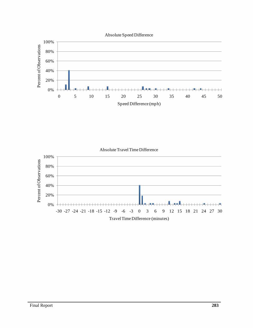
Final Report 283

0%

20%

40%

60%

80%

100%

0 5 10 15 20 25 30 35 40 45 50

Perc

ent o

f Obs

erva

tions



0%

20%

40%

60%

80%

100%

-30 -27 -24 -21 -18 -15 -12 -9 -6 -3 0 3 6 9 12 15 18 21 24 27 30

Perc

ent o

f Obs

erva

tions



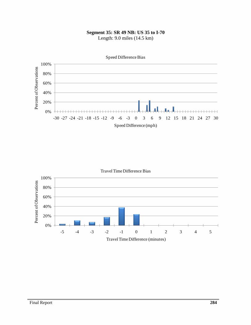
Final Report 284

Segment 35: SR 49 NB: US 35 to I-70 Length: 9.0 miles (14.5 km)

0%

20%

40%

60%

80%

100%

-30 -27 -24 -21 -18 -15 -12 -9 -6 -3 0 3 6 9 12 15 18 21 24 27 30

Perc

ent o

f Obs

erva

tions



0%

20%

40%

60%

80%

100%

-5 -4 -3 -2 -1 0 1 2 3 4 5

Perc

ent o

f Obs

erva

tions



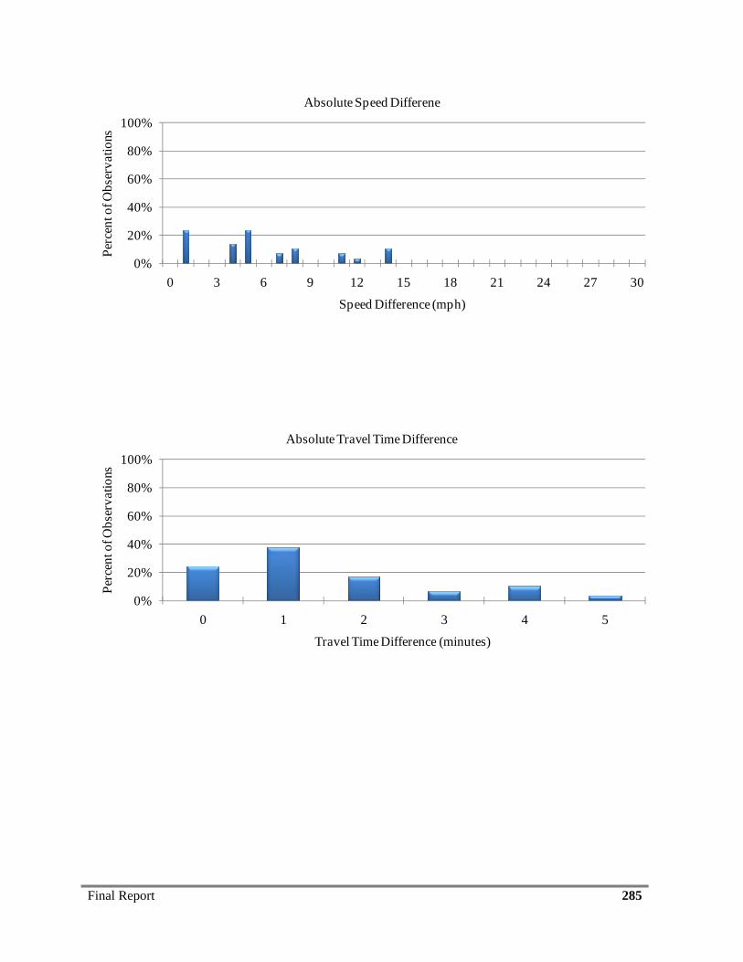
Final Report 285

0%

20%

40%

60%

80%

100%

0 3 6 9 12 15 18 21 24 27 30

Perc

ent o

f Obs

erva

tions


Absolute Speed Differene

0%

20%

40%

60%

80%

100%

0 1 2 3 4 5

Perc

ent o

f Obs

erva

tions



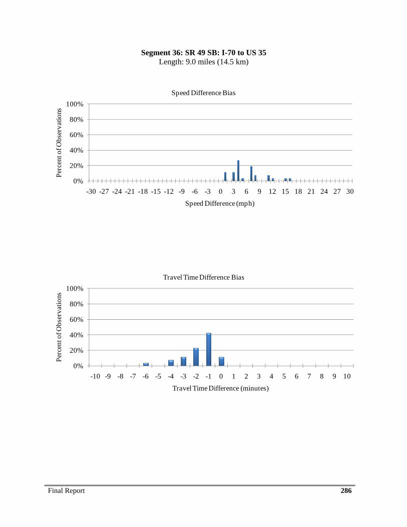
Final Report 286

Segment 36: SR 49 SB: I-70 to US 35 Length: 9.0 miles (14.5 km)

0%

20%

40%

60%

80%

100%

-30 -27 -24 -21 -18 -15 -12 -9 -6 -3 0 3 6 9 12 15 18 21 24 27 30

Perc

ent o

f Obs

erva

tions



0%

20%

40%

60%

80%

100%

-10 -9 -8 -7 -6 -5 -4 -3 -2 -1 0 1 2 3 4 5 6 7 8 9 10

Perc

ent o

f Obs

erva

tions



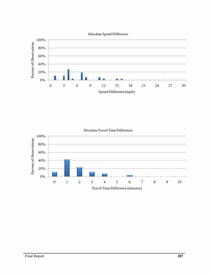
Final Report 287

0%

20%

40%

60%

80%

100%

0 3 6 9 12 15 18 21 24 27 30

Perc

ent o

f Obs

erva

tions



0%

20%

40%

60%

80%

100%

0 1 2 3 4 5 6 7 8 9 10

Perc

ent o

f Obs

erva

tions



Documents

Statistical Validation of Speeds and Travel Times Provided by a