Dam Removal Express Assessment Models (DREAM). Part 1: Model

Journal of Hydraulic Research Vol. 0, No. 0 (2005), pp. 1–17

© 2005 International Association of Hydraulic Engineering and Research

Dam Removal Express Assessment Models (DREAM). Part 1: Model developmentand validation

YANTAO CUI, Ph.D., Hydraulic Engineer, Stillwater Sciences, 2855 Telegraph Ave., Suite 400, Berkeley, CA 94705, USA.Tel.: 510-848-8098; fax: 510-848-8398; e-mail: [email protected] (author for correspondance)

GARY PARKER, St. Anthony Falls Laboratory, University of Minnesota, Mississippi River at Third Avenue S.E.,Minneapolis, MN 55414, USA

CHRISTIAN BRAUDRICK, Department of Earth and Planetary Sciences, University of California, 301 McCone Hall,Berkeley, CA 94720, USA

WILLIAM E. DIETRICH, Department of Earth and Planetary Sciences, University of California, 301 McCone Hall,Berkeley, CA 94720, USA

BRIAN CLUER, NOAA Fisheries, 777 Sonoma Avenue, Santa Rosa, CA 95404, USA

ABSTRACTMany dams have been removed in the recent decades in the U.S. for reasons including economics, safety, and ecological rehabilitation. More damsare under consideration for removal; some of them are medium to large-sized dams filled with millions of cubic meters of sediment. Reaching adecision to remove a dam and deciding as how the dam should be removed, however, are usually not easy, especially for medium to large-sized dams.One of the major reasons for the difficulty in decision-making is the lack of understanding of the consequences of the release of reservoir sedimentdownstream, or alternatively the large expense if the sediment is to be removed by dredging. This paper summarizes the Dam Removal ExpressAssessment Models (DREAM) developed at Stillwater Sciences, Berkeley, California for simulation of sediment transport following dam removal.There are two models in the package: DREAM-1 simulates sediment transport following the removal of a dam behind which the reservoir depositis composed primarily of non-cohesive sand and silt, and DREAM-2 simulates sediment transport following the removal of a dam behind whichthe upper layer of the reservoir deposit is composed primarily of gravel. Both models are one-dimensional and simulate cross-sectionally and reachaveraged sediment aggradation and degradation following dam removal. DREAM-1 is validated with a set of laboratory experiments; its reservoirerosion module is applied to the Lake Mills drawdown experiment. DREAM-2 is validated with the field data for a natural landslide. Sensitivity testsare conducted with a series of sample runs in the companion paper, Cui et al. (2006), to validate some of the assumptions in the model and to provideguidance in field data collection in actual dam removal projects.

RÉSUMÉ

Keywords:

1 Introduction

Citing the U.S.Army Corps of Engineers, the Bureau of Reclama-tion, the Tennessee Valley Authority and other U.S. sources, The

Revision received

1

Guidelines for Retirement of Dams and Hydroelectric Facilities(the Guidelines hereafter, ASCE, 1997) state that there were morethan 75,000 dams in the U.S. in 1996. The majority of thesedams were built before the late 1960s, and are now approaching

2 Cui et al.

or exceeding their average designed life expectancy of about50 years. In light of the aging of these facilities and in light ofeconomic and ecological considerations, some dams have beendecommissioned and removed, and many more will be removedin the future. As pointed out in the Guidelines, the key element in adam removal project is usually sediment management, which nor-mally constitutes more than a third of the total dam removal cost.The Guidelines listed three sediment management options asso-ciated with dam removal: river erosion, mechanized removal, andstabilization, each with different advantages and disadvantages.Overall, mechanized removal has the least impact on the down-stream geomorphic/ecological system but has the highest cost. Incontrast to mechanized removal, the river erosion option has thegreatest downstream impact but the lowest cost. Within each indi-vidual option, there may be many implementation alternatives,and each of them may have different downstream impacts andproject costs. In the river erosion option, for example, the dam canbe partially or completely removed by either a one-shot removal(i.e., to remove the entire dam before reservoir sediment deposit isallowed to erode and transport downstream) or a staged removal.The choice of a removal method among available options andthe variety of design alternatives within an option are largelydetermined by the predicted downstream impacts of the sedimentrelease, as well as the confidence level of the predictions.

Because dam removal is a relatively recent issue, and becauseof the complexities involved in sediment transport following damremoval, a sediment transport model designed to simulate damremoval and the eventual fate of the reservoir sediment has notbeen available to the public. Instead, engineers and geomor-phologists have been using sediment transport models that weredeveloped for other purposes to address the problem. For exam-ple, HEC-6, in combination with several other reservoir erosionmodels, was used to model the proposed removal of the Elwhaand Glines Canyon Dams on the Elwha River, WA (Bureau ofReclamation, 1996b). The problem with such a modeling exer-cise is that the sediment transport model used for simulation,HEC-6 in this particular case, was not developed for simula-tion following the removal of a dam, and thus is not capableof simulating the steep slope in the vicinity of the dam imme-diately following removal. A practice modelers have adoptedto overcome such problems is to model the reaches upstreamand downstream of the dam separately. That is, reservoir erosionupstream of the dam is simulated independently, and the resultsare used to define the upstream boundary condition for the sim-ulation of the downstream reach (e.g., Bureau of Reclamation,1996b). This practice, however, is valid only if part of the dam isstill in place and the upstream and downstream reaches of the damare still separated by the remaining portion of the dam. That is, thecombined models cannot be used for the simulation of a one-shotremoval, nor can they be used for simulation of the later stages ina staged removal. In such cases, the deposition downstream of thedam greatly affects the erosion and transport of sediment in andupstream of the reservoir, and thus the independent simulation ofreservoir erosion upstream of the dam becomes invalid.

To simulate the potential removal of Soda Springs Dam on theNorth Umpqua River, OR, and Marmot Dam on the Sandy River,OR, Stillwater Sciences developed two customized numerical

models that specifically address the sediment transport issuesfollowing the removal of the dams (Stillwater Sciences, 1999,2000; Cui and Wilcox, 2005) based on the sediment pulse workof Cui and Parker (2005). In the Soda Springs Dam case, thereservoir deposit is composed primarily of sand and silt, andthe river downstream of the dam is a high-gradient bedrock-dominated gravel-bedded channel (Stillwater Science, 1999).In the Marmot Dam case, the reservoir deposit is stratified,with the upper layer of the deposit composed of a mixtureof gravel and sand, and the lower layer composed of primar-ily sand and silt. The Sandy River downstream of MarmotDam is a high-gradient bedrock-dominated gravel-bedded river,with a gradual transition further downstream to a lower-gradientgravel-bedded river (Stillwater Sciences, 2000; Cui and Wilcox,2005).

The Dam Removal Express Assessment Models (DREAM)presented in this paper are modified from the Soda SpringsDam and the Marmot Dam models: DREAM-1 is designedfor the simulation of sediment transport following the removalof a dam behind which the reservoir deposit is composedprimarily of non-cohesive sand and silt, and DREAM-2 isdesigned for the simulation of sediment transport following theremoval of a dam behind which the upper layer of the reservoirdeposit is composed primarily of gravel. Channel characteris-tics can include any combination of bedrock, gravel-bedded andsand-bedded rivers for a DREAM-1 simulation, and a combi-nation of bedrock and gravel-bedded rivers for a DREAM-2simulation.

The Marmot Dam removal model (Cui and Wilcox, 2005) dif-fers from the generic model of Cui and Parker (2005) in thatCui and Parker (2005) assumes gravel-bedded without geolog-ical controls such as bedrock outcrops while Cui and Wilcox(2005) allows such geological controls. The implication is thatthe pre-disturbance bedload transport in Cui and Parker (2005)is at capacity while the pre-dam-removal condition in Cui andWilcox (2005) can be under-capacity. The other major differencebetween Cui and Parker (2005) and Cui and Wilcox (2005) is thatCui and Parker (2005) considers only bedload transport, while theMarmot Dam removal model (Cui and Wilcox, 2005) considersthe transport of both gravel and sand. In addition, Cui and Parker(2005) uses only one discharge station for input to the model andassumes that the discharge at any cross section is proportional tothe local drainage area. The Marmot Dam removal model (Cuiand Wilcox, 2005) allows any number of hydrologic stations, andthe discharge at each cross section can be linked to one of thosestations.

The major improvement of DREAM-1 over the Soda SpringsDam removal model (Stillwater Sciences, 1999) is that the currentmodel assumes trapezoidal cross sections in the reach upstream ofthe dam, and allows channel widening due to the erosion of bothbanks during the period of downcutting of the reservoir deposit,while the Soda Springs Dam removal model (Stillwater Sciences,1999) assumes set rectangular cross sections for the entire riverreach. This improvement is also reflected in DREAM-2 pre-sented in this paper as compared to the Marmot Dam removalmodel (Cui and Wilcox, 2005). In addition, the gravel and sandtransport models are built as an integrated model in DREAM-2,

Dam Removal Express Assessment Models 3

although gravel and sand transport capacities are still calculatedseparately with their respective equations, representing anothermajor improvement over the Marmot Dam removal model (Cuiand Wilcox, 2005), in which the gravel model is run indepen-dently and the resulting fine sediment erosion from the reservoirdeposit is used as input to the sand model. The integration ofgravel and sand transport into a single model allows the fine sed-iment generated from gravel abrasion to be accounted for. Theintegrated model also allows accounting for the fine sedimentdeposited in the interstices of gravel deposits.

In addition to these major improvements of the currentmodels over the previous models, this paper and the com-panion paper, Y. Cui, C. Braudrick, W.E. Dietrich, B. Cluerand G. Parker (unpublished data) focus on different issuesof interest from (a) those in Cui and Parker (2005), whichfocuses on the relative importance of gravel abrasion on theevolution of gravel pulses in mountain rivers, and (b) thosein Cui and Wilcox (2005), which presents a case study ofa dam removal project. This and the companion paper, Cuiet al. (2006), focus on: (a) the development of the two mod-els and the underlying assumptions, with special attentionto the reservoir erosion module; (b) validation of the mod-els with field and laboratory data; and (c) sensitivity tests tomajor fixed and user-defined parameters, which provide guid-ance for future model applications and field data collection,and provide a reference for development of similar modelsin the future.

2 Hypotheses on the morphologic adjustments andsediment transport processes following dam removaland governing equations

Many small dams have been removed in the U.S. and around theworld with very little documentation. Removal of medium- tolarge-sized dams is very rare, and no documentation of morpho-logical adjustments and sediment transport processes associatedwith such cases was found. In order to develop the DREAM,we hypothesized the following morphologic adjustments andsediment transport processes following a dam removal.

Consider a dam, behind which the reservoir area is either fullyor partially filled with non-cohesive sediment, which is in the pro-cess of being analyzed for removal. To begin the dam removalprocess, as much water as possible is drained out of the reservoirduring the low flow season and a cofferdam is constructed at acertain distance upstream of the dam to divert the flow away fromthe dam. With the protection from the cofferdam, the sedimentbetween the dam and the cofferdam is excavated to expose andeventually remove the dam. The dam can be a one-time completeremoval (one-shot removal), a partial removal across the dam, orthe opening of a notch at the dam. The cofferdam is then artifi-cially or naturally breached at a design discharge after the damand other facilities are physically removed. In case of opening anotch on the dam, it is assumed that no flow control structure isinstalled on the notch, i.e. free-surface flow is maintained at alltimes. The regulated (gated) notch such as in one of the options for

the proposed Glines Canyon Dam removal (Bureau of Reclama-tion, 1996a) cannot be modeled with the current model withoutsite-specific modification to the code.

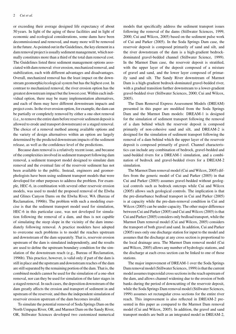
Note that the sediment deposit in the reservoir following theremoval of the dam and before the breaching of the cofferdam hassteep slope facing downstream (often at the angle of repose), asdemonstrated in the sketch in Fig. 1(a). The sketches in Figure 1are vertically exaggerated, and as a result, the above slope appearsmuch steeper than the angle of repose. This steep slope allowsfor quick erosion of the reservoir sediment and its subsequentdeposition downstream as a fan-delta as soon as the cofferdamis breached. The rapid downcutting of the reservoir deposit verylikely drains the flow from any existing secondary channels, thuspreventing further downcutting and leaving them perched. As aresult, it is very likely that only one channel is formed in the reser-voir deposit following the removal of the dam. Due to the lack offield data, it is not clear how wide a channel develops in the reser-voir reach. It is reasonable, however, to assume that the activechannel will have a geometry similar to that found in the reachimmediately downstream of the dam. Also because the channelwill tend to cut down rapidly, it will very likely experience rela-tively minor lateral migration. Depending on the relative widthsof the reservoir deposit and the active channel, part of the reser-voir deposit may not be eroded and transported downstream evenif the channel reaches its pre-dam gradient. This deposit remains

Figure 1 Sketch of the typical geomorphic characteristics of a damremoval project.

4 Cui et al.

in the form of terraces. Once the channel reaches a relativelystable gradient and the degradation rate falls off, the channelmay begin to migrate laterally and to erode these terraces. Fig-ure 1(b) shows a sketch of a river after dam removal that is stilladjusting its gradient. In case the upper layer of the reservoirdeposit is composed of primarily coarse sediment (gravel, peb-bles, and boulders), it is reasonable to assume that the erosionof the reservoir deposit is governed by gravel transport becauseof the relatively smaller transport capacity of coarse sedimentcompared to that of sand.

The above hypotheses are incorporated into the DREAM pre-sented below. The possible lateral migration once the channelreaches a relatively stable gradient, however, is not implementedin the models.

A unique feature of sediment transport modeling followingdam removal is the steep slope in the vicinity of the dam shortlyafter dam removal. Simulation with a steep slope requires that themodel be capable of simulating sub-critical, super-critical, andtransient flows.

Many existing numerical models of mobile-bed open-channelflow are equipped with the ability to simulate sub-critical,super-critical, and transient flows (e.g. Li et al., 1988; Rahuelet al., 1989; Holly and Rahuel, 1990a,b; Bhallamudi andChaudhry, 1991; US Army Corps of Engineers, 1993; Cui et al.,1996, 2003b; Cui and Parker, 1997, 2005). With appropriatemodifications, those models should be capable of simulatingsediment transport processes following a dam removal. Thesame procedure as used in Cui and Parker (2005) and Cuiand Wilcox (2005) is applied in the flow simulation describedbelow.

For the purpose of flow calculation, the channel is assumed tobe rectangular with width equal to the local bankfull width, andflow parameters are calculated with a combination of a standardbackwater calculation and the quasi-normal flow assumption,

dh

dx= S0 − Sf

1 − F 2, F < 0.9

S0 = Sf , F ≥ 0.9(1a)

in which h denotes water depth; x denotes downstream distance;S0 denotes channel bed slope; Sf denotes friction slope; andF denotes the Froude number;

S0 = − ∂(ηb + ηg + ηs)

∂x(2)

F 2 = Q2w

gB2h3(3)

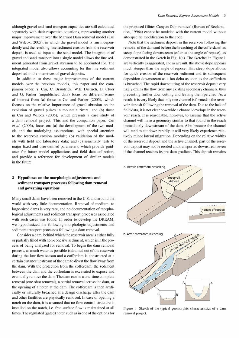
in which ηb denotes the elevation of non-erodible material such asbedrock; ηg denotes the thickness of the gravel deposit; ηs denotesthe thickness of any sand deposit on top of gravel deposit or thenon-erodible material; Qw denotes water discharge; g denotesacceleration of gravity; and B denotes bankfull channel width.It should be noted that bankfull channel width upstream of thedam site follow dam removal is assumed to be equal to the aver-age bankfull width within a short distance downstream of thedam. The friction slope Sf will be discussed later in conjunc-tion with the discussion of sediment transport equation. A sketch

ηb

ηg

h

water surface

channel bed

the base

flow direction

gravel deposit (above the base)

material that cannot or will not be eroded by the flow

sand deposit

ηs

Figure 2 Sketch defining some of the terms used in the models.

illustrating these definitions is given as Fig. 2. It needs to be clari-fied that the thickness of gravel deposit, ηg, should be consideredas constant in a DREAM-1 simulation based on the assumptionthat the aggradation and degradation of the gravel bed is rela-tively slow compared to the transport of sand. This assumption isnot used in DREAM-2, which calculates gravel as well as sandtransport.

Cui and Parker (1997) show that the quasi-normal assumptionprovides a good approximation of the full backwater equationsfor flows with high Froude number. Cui and Parker (2005) usethis finding to simulate the evolution of sediment pulses in moun-tain rivers. In Cui and Parker (2005), the flow is calculated withthe backwater equation whenever local Froude number is lowerthan 0.75, and with quasi-normal assumption otherwise. Theirsimplified treatment enables them to model the sub-critical flowupstream of the sediment pulse, the super-critical flow at the steepdownstream face of the sediment pulse, and the transient flowslinking the two states.

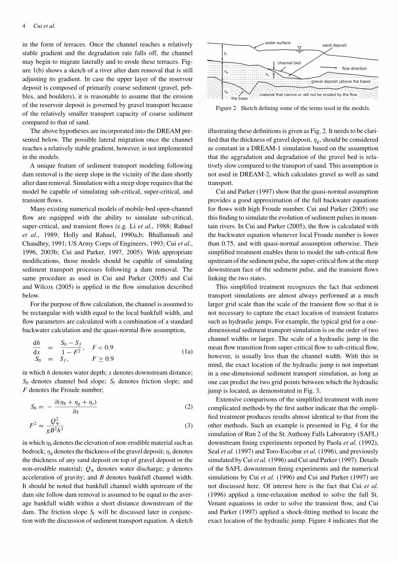
This simplified treatment recognizes the fact that sedimenttransport simulations are almost always performed at a muchlarger grid scale than the scale of the transient flow so that it isnot necessary to capture the exact location of transient featuressuch as hydraulic jumps. For example, the typical grid for a one-dimensional sediment transport simulation is on the order of twochannel widths or larger. The scale of a hydraulic jump in themean flow transition from super-critical flow to sub-critical flow,however, is usually less than the channel width. With this inmind, the exact location of the hydraulic jump is not importantin a one-dimensional sediment transport simulation, as long asone can predict the two grid points between which the hydraulicjump is located, as demonstrated in Fig. 3.

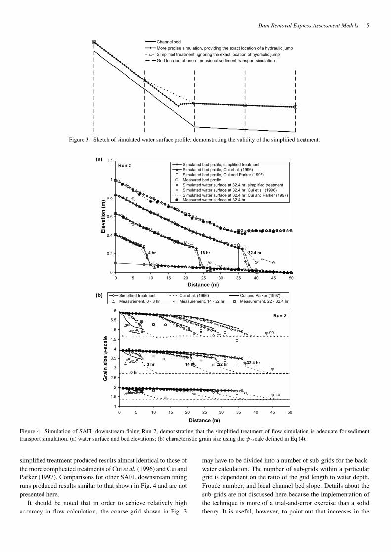
Extensive comparisons of the simplified treatment with morecomplicated methods by the first author indicate that the simpli-fied treatment produces results almost identical to that from theother methods. Such an example is presented in Fig. 4 for thesimulation of Run 2 of the St. Anthony Falls Laboratory (SAFL)downstream fining experiments reported by Paola et al. (1992),Seal et al. (1997) and Toro-Escobar et al. (1996), and previouslysimulated by Cui et al. (1996) and Cui and Parker (1997). Detailsof the SAFL downstream fining experiments and the numericalsimulations by Cui et al. (1996) and Cui and Parker (1997) arenot discussed here. Of interest here is the fact that Cui et al.(1996) applied a time-relaxation method to solve the full St.Venant equations in order to solve the transient flow, and Cuiand Parker (1997) applied a shock-fitting method to locate theexact location of the hydraulic jump. Figure 4 indicates that the


Channel bedMore precise simulation, providing the exact location of a hydraulic jumpSimplified treatment, ignoring the exact location of hydraulic jumpGrid location of one-dimensional sediment transport simulation

Figure 3 Sketch of simulated water surface profile, demonstrating the validity of the simplified treatment.

0

0.2

0.4

0.6

0.8

1

1.2

0 5 10 15 20 25 30 35 40 45 50

Distance (m)

Ele

vati

on

(m

)

Simulated bed profile, simplified treatmentSimulated bed profile, Cui et al. (1996)Simulated bed profile, Cui and Parker (1997)Measured bed profileSimulated water surface at 32.4 hr, simplified treatmentSimulated water surface at 32.4 hr, Cui et al. (1996)Simulated water surface at 32.4 hr, Cui and Parker (1997)Measured water surface at 32.4 hr

Run 2

4 hr 16 hr 32.4 hr

(a)

1

1.5

2

2.5

3

3.5

4

4.5

5

5.5

6

0 5 10 15 20 25 30 35 40 45 50

Distance (m)

Gra

in s

ize

ψ-s

cale

Simplified treatment Cui et al. (1996) Cui and Parker (1997)Measurement, 0 - 3 hr Measurement, 14 - 22 hr Measurement, 22 - 32.4 hr

Run 2

ψ-90

ψ-10

0 hr

3 hr 14 hr 22 hr 32.4 hr

(b)

ψ

Figure 4 Simulation of SAFL downstream fining Run 2, demonstrating that the simplified treatment of flow simulation is adequate for sedimenttransport simulation. (a) water surface and bed elevations; (b) characteristic grain size using the ψ-scale defined in Eq (4).

simplified treatment produced results almost identical to those ofthe more complicated treatments of Cui et al. (1996) and Cui andParker (1997). Comparisons for other SAFL downstream finingruns produced results similar to that shown in Fig. 4 and are notpresented here.

It should be noted that in order to achieve relatively highaccuracy in flow calculation, the coarse grid shown in Fig. 3

may have to be divided into a number of sub-grids for the back-water calculation. The number of sub-grids within a particulargrid is dependent on the ratio of the grid length to water depth,Froude number, and local channel bed slope. Details about thesub-grids are not discussed here because the implementation ofthe technique is more of a trial-and-error exercise than a solidtheory. It is useful, however, to point out that increases in the

6 Cui et al.

ratio of grid length to water depth, Froude number, or local chan-nel bed slope should normally result in an increase in the numberof sub-grids within the grid in order to achieve a similar relativeaccuracy at all the grid points as illustrated in Fig. 3.

For the purpose of sediment mass conservation calculations,the channel downstream of the dam is assumed to have the samerectangular cross-sections as those used in flow calculation. TheExner equations of sediment continuity for the reach downstreamof the dam used here have been modified from Cui and Parker(2005), which in turn have their origins in continuous forms inParker (1991a,b). Similar but simpler forms of the Exner equa-tions have been used in Parker (1990b), Cui and Parker (1998)and Cui and Wilcox (2005).

Since sediment transport of gravel is computed on a grain size-specific basis, it is first necessary to specify the discretization ofthe gravel grain size distribution. Here “gravel” means gravel andcoarser sizes. Grain size D can be equivalently characterized interms of the (base-2) logarithmic ψ-scale;

ψ = −φ = log2(D) (4)

In the above relation φ denotes the φ-scale familiar to sedimen-tologists. Gravel grain size distributions are discretized into Nbins j = 1, . . . , N bounded by N + 1 grain sizesD1, . . . , DN+1

(ψ1, . . . , ψN+1) progressing from smaller to larger size withincreasing j. Here D1 always corresponds to 2 mm (i.e. a valueof ψ1 of 1), i.e. the border between sand and gravel. The jthgrain size range is bounded by the sizes Dj and Dj+1, and hasthe characteristic size

D̄j = √DjDj+1, ψ̄j = log2(D̄j) = 1

2

(ψ̄j + ψ̄j+1

)(5a,b)

The fraction of the deposit that is gravel is denoted as fg and thefraction that is sand is denoted as fs. The two need not add upto unity due to the possible presence of silt in the deposit. Thefractions of the gravel in the surface layer of the stream and thebedload in the jth grain size range are denoted respectively asFj , and pj , where both are normalized to sum to unity over allgravel sizes. The formulation presented below also uses surfacefractions F ′

j that have been adjusted according to Parker (1991a)to reflect exposed surface area available for abrasion;

F ′j =

Fj

/√D̄j

∑Fj

/√D̄j

(6)

The Exner equation for the total gravel load (bedload) for thereach downstream of the dam is

(1 − λp)fgB∂ηg

∂t+ ∂Qg

∂x

+ βQg

(2 + 1

3 ln(2)

p1 + F ′1

ψ2 − ψ1

)= qgl (7)

The Exner equation for gravel (bedload) of an individual grainsize range (the jth size range) for the reach downstream of thedam is

(1 − λp)fgB

(∂(LaFj)

∂t+ fIj

(ηg − La)

∂t

)+ ∂(Qgpj)

∂x

+ βQg(pj + F ′

j

) + βQg

3 ln(2)(pj + F ′

j

ψj+1 − ψj− pj+1 + F ′

j+1

ψj+2 − ψj+1

)= qglj (8)

The Exner equation for sand for the reach downstream of thedam is

(1 − λp)B

(∂ηs

∂t+ fs

∂ηg

∂t

)+ ∂Qs

∂x− βQg

3 ln(2)

p1 + F ′1

ψ2 − ψ1= qsl

(9)

In the above relations λp denotes the porosity of the deposit;t denotes time; Qg denotes volumetric transport rate of gravel(bedload); x denotes downstream distance; β denotes volumetricabrasion coefficient of gravel (bedload); qgl denotes lateral gravel(bedload) supply rate per unit distance (i.e., volume of bedloadsupplied to the river per unit time per unit distance from tributariesand bank erosion); La denotes the active layer (surface layer)thickness, which is assumed to be a constant value of 0.5 m forsimplicity and is discussed in Run 2 of the sample runs in thecompanion paper, Cui et al. (2006); qglj denotes lateral gravel(bedload) supply rate per unit distance in the jth size range; Qs

denotes volumetric transport rate of sand; and qsl denotes thelateral sand supply rate per unit distance. In addition, fIj denotesthe fraction in the jth size range of the gravel that is exchangedbetween the channel bed and bedload as the channel aggrades ordegrades. A relation for fIj is provided below.

The derivation of Eqs (7)–(9) and an explanation of the termsin the equations are not presented in this paper. Interested readersshould be able to derive those equations in reference to similarequations in Parker (1991a,b) and Cui and Parker (1998).

It should be noted that the full set of Eqs (7)–(9) apply toDREAM-2, in which both gravel and sand transport are mod-eled. In case of modeling with DREAM-1, it is assumed thatgravel transport is insignificant compared to sand transport, andthus, Eqs (7) and (8) become irrelevant. Furthermore, Eq. (9) issimplified as

(1 − λp)B∂ηs

∂t+ ∂Qs

∂x= qsl (10)

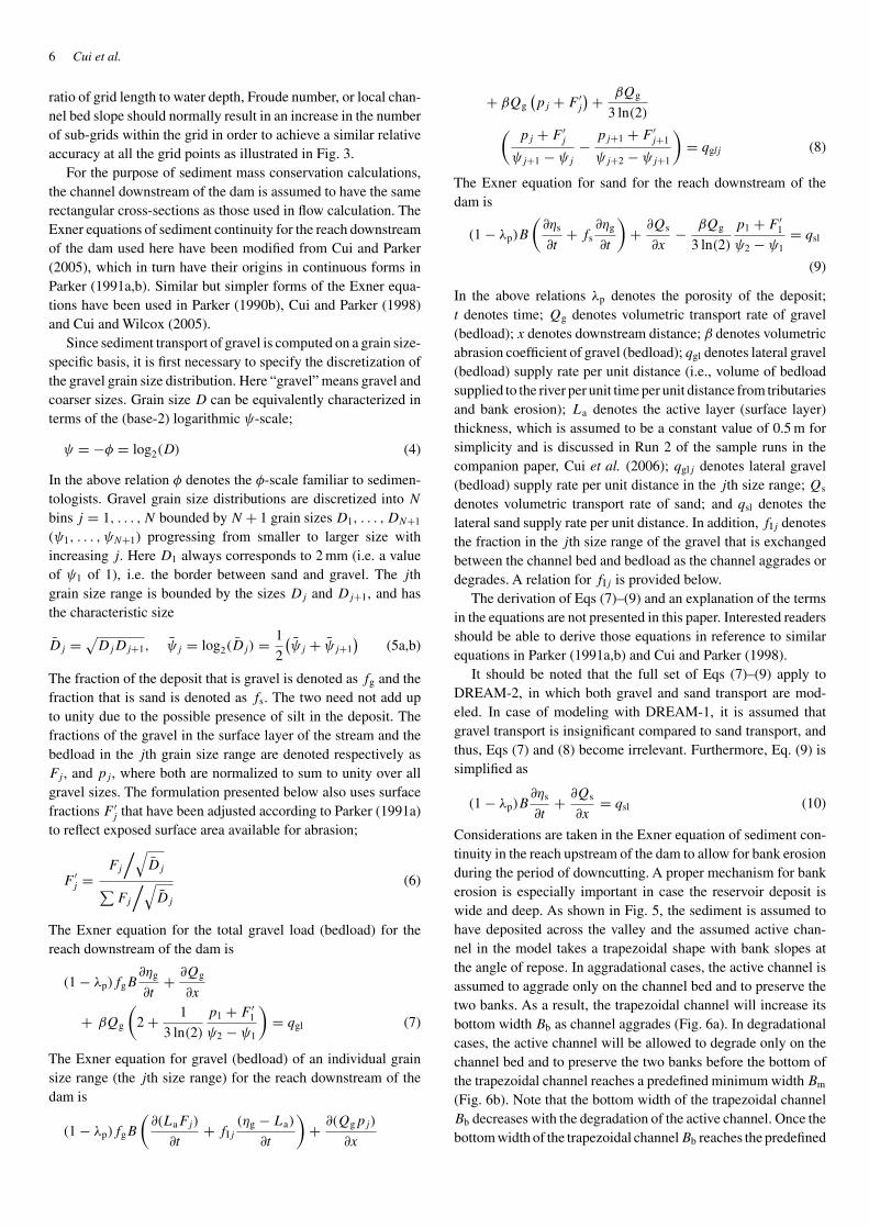
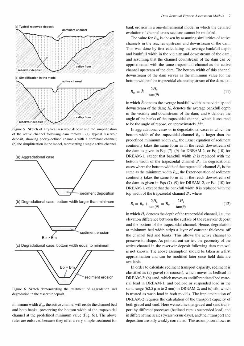
Considerations are taken in the Exner equation of sediment con-tinuity in the reach upstream of the dam to allow for bank erosionduring the period of downcutting. A proper mechanism for bankerosion is especially important in case the reservoir deposit iswide and deep. As shown in Fig. 5, the sediment is assumed tohave deposited across the valley and the assumed active chan-nel in the model takes a trapezoidal shape with bank slopes atthe angle of repose. In aggradational cases, the active channel isassumed to aggrade only on the channel bed and to preserve thetwo banks. As a result, the trapezoidal channel will increase itsbottom width Bb as channel aggrades (Fig. 6a). In degradationalcases, the active channel will be allowed to degrade only on thechannel bed and to preserve the two banks before the bottom ofthe trapezoidal channel reaches a predefined minimum width Bm

(Fig. 6b). Note that the bottom width of the trapezoidal channelBb decreases with the degradation of the active channel. Once thebottom width of the trapezoidal channelBb reaches the predefined


(a) Typical reservoir deposit

(b) Simplification in the model

dominant channel

active channel

reservoir deposit

reservoir deposit

valley floor

valley floor

Figure 5 Sketch of a typical reservoir deposit and the simplificationof the active channel following dam removal. (a) Typical reservoirdeposit, showing poorly-defined channels with a dominant channel;(b) the simplification in the model, representing a single active channel.

(a) Aggradational case

(b) Degradational case, bottom width larger than minimuml

(c) Degradational case, bottom width equal to minimuml

sediment deposition

sediment erosion

sediment erosion

Bb > Bm

Bb = Bm

Figure 6 Sketch demonstrating the treatment of aggradation anddegradation in the reservoir deposit.

minimum widthBm, the active channel will erode the channel bedand both banks, preserving the bottom width of the trapezoidalchannel at the predefined minimum value (Fig. 6c). The aboverules are enforced because they offer a very simple treatment for

bank erosion in a one-dimensional model in which the detailedevolution of channel cross-sections cannot be modeled.

The value for Bm is chosen by assuming similarities of activechannels in the reaches upstream and downstream of the dam.This was done by first calculating the average bankfull depthand bankfull width in the vicinity and downstream of the dam,and assuming that the channel downstream of the dam can beapproximated with the same trapezoidal channel as the activechannel upstream of the dam. The bottom width of this channeldownstream of the dam serves as the minimum value for thebottom width of the trapezoidal channel upstream of the dam, i.e.,

Bm = B̄ − 2H̄b

tan(θ)(11)

in which B̄ denotes the average bankfull width in the vicinity anddownstream of the dam; H̄b denotes the average bankfull depthin the vicinity and downstream of the dam; and θ denotes theangle of the banks of the trapezoidal channel, which is assumedto be the angle of repose, or approximately 35◦.

In aggradational cases or in degradational cases in which thebottom width of the trapezoidal channel Bb is larger than thepredefined minimum width Bm, the Exner equation of sedimentcontinuity takes the same form as in the reach downstream ofthe dam as given in Eqs (7)–(9) for DREAM-2, or Eq (10) forDREAM-1, except that bankfull width B is replaced with thebottom width of the trapezoidal channel Bb. In degradationalcases where the bottom width of the trapezoidal channelBb is thesame as the minimum width Bm, the Exner equation of sedimentcontinuity takes the same form as in the reach downstream ofthe dam as given in Eqs (7)–(9) for DREAM-2, or Eq. (10) forDREAM-1, except that the bankfull width B is replaced with thetop width of the trapezoidal channel Bt , where

Bt = Bb + 2Hd

tan(θ)= Bm + 2Hd

tan(θ)(12)

in whichHd denotes the depth of the trapezoidal channel, i.e., theelevation difference between the surface of the reservoir depositand the bottom of the trapezoidal channel. Hence, degradationat minimum bed width strips a layer of constant thickness offthe channel bed and banks. This allows the active channel topreserve its shape. As pointed out earlier, the geometry of theactive channel in the reservoir deposit following dam removalis not known. The above assumption should be taken as a firstapproximation and can be modified later once field data areavailable.

In order to calculate sediment transport capacity, sediment isclassified as (a) gravel (or coarser), which moves as bedload inDREAM-2; (b) sand, which moves as undifferentiated bed mate-rial load in DREAM-1, and bedload or suspended load in thesand range (62.5 µm to 2 mm) in DREAM-2; and (c) silt, whichis treated as wash load in both models. The implementation ofDREAM-2 requires the calculation of the transport capacity ofboth gravel and sand. Here we assume that gravel and sand trans-port by different processes (bedload versus suspended load) andin different time scales (years versus days), and their transport anddeposition are only weakly correlated. This assumption allows us

8 Cui et al.

to use their respective transport equations to evaluate gravel andsand transport capacities in the model. The recent developmentin unified gravel/sand transport equations (e.g., Wilcock 1997,1998; Wilcock and Crowe, 2003) can be implemented into themodel in the future.

The sediment transport equation employed for calculation ofsand transport capacity in DREAM- 1 and DREAM-2 is the bedmaterial equation of Brownlie (1982), which was empiricallyderived from a very large database of flume experiments andfield measurements. The application of Brownlie’s bed materialequation (Brownlie, 1982) requires the coupling of the sedimenttransport equation with a friction formulation. Brownlie (1982)classified the flow into lower and upper flow regimes, and fric-tion formulations were given for each regime. The lower regimecorresponds to a state with ripple and dune bedforms and upperregime corresponds to the plane bed or antidune state. An upperlimit for lower regime and a lower limit for upper regime areprovided in Brownlie (1982), and the actual transition betweenthe two regimes is dependent on whether the flow stage is risingor falling. Because the model applies the daily average dischargerecord as model input, the specifics about whether the flow isrising or falling are not included in the use of the Brownlie’sformulation, and as a result, the average of the upper limit ofthe lower regime and the lower limit of the upper regime is usedto define the transition between the two regimes in the model.In addition, in applying the bed material equation of Brownlie(1982) and its associated friction formulations, the median grainsize is replaced with geometric mean grain size because (a) geo-metric mean grain size is usually very close to the median size;(b) geometric mean grain size is usually more representative ofthe characteristics of a grain size distribution; and (c) geometricmean grain size is relatively easy to calculate because it elimi-nates the interpolation process in a median grain size calculation.Versions of the Brownlie equations that are slightly modified inthis way have been presented in Cui and Wilcox (2005) and arenot described here.

Brownlie’s bed material load equation calculates the transportcapacity of bed material, which is usually composed primarilyof sand and can be transported either as bedload or suspendedload. Finer particles such as silt and clay are considered as washload, which can be supplied from upstream and tributaries, and isassumed not to be deposited onto the channel bed. The wash loaddeposited in the reservoir during the period of dam operation isassumed to be entrained into the water column and transporteddownstream without re-deposition once it is exposed to the flow.Given the importance of distinguishing the suspended load fromthe total load in order to assess potential biologically signifi-cant sediment concentrations in suspension, the portion of thebed material load that is in suspension is calculated using thefollowing criterion (e.g., van Rijn, 1984):

vs

κu∗< 1 (13)

where vs is particle settling velocity calculated with the proceduregiven by Dietrich (1982); κ is the von Karman constant with avalue of 0.4, and u∗ denotes shear velocity.

The sediment transport equation employed for calculation ofgravel transport capacity in DREAM-2 is the surface-based bed-load equation of Parker (1990a,b). Parker’s bedload equation(Parker, 1990a,b) calculates bedload transport rate and grain sizedistribution based on the local surface grain size distribution andshear stress. Details of the surface-based bedload equation ofParker (1990a,b) are not presented here; interested readers arereferred to the original publications (e.g., Parker, 1990a,b).

Parker (1990a,b) suggested that a Keulegan type of resistancerelation be used in conjunction to his surface-based bedload equa-tion, by assuming the roughness height as twice the surface grainsize D90. Cui et al. (1996) slightly modified the resistance rela-tion suggested by Parker (1990a,b) by replacing the roughnessheight ks with

ks = 2Dsgσ1.28sg (14)

in which Dsg and σsg denote the surface geometric mean andgeometric standard deviation, respectively. It should be notedthat sand is excluded from the surface grain size distribution incalculating Dsg and σsg values. The slightly modified resistancerelation (Cui et al., 1996) has been employed in the models ofCui and Parker (1997, 1998, 2005), Cui et al. (2003b), and Cuiand Wilcox (2005).

It should be noted that there are two sets of resistance rela-tions in DREAM-2; the modified resistance relation of Brownlie(1982) in calculating sand transport capacity and the Keulegantype relation in calculating gravel transport capacity. Realizingthat the channel bed is primarily gravel-bedded in a DREAM-2simulation, the Keulegan type of resistance relation is used forsimulation of flow at all times in implementing DREAM-2.

Application of sediment continuity equation in DREAM-2also needs a relation to link the grain size distributions in bedloadand the channel bed (e.g., surface layer and substrate). The rela-tions applied in DREAM-2 is the same as that in Cui and Parker(2005) and in the Marmot Dam removal model (Cui and Wilcox,2005):

fIj ={fbj, ∂ηg/∂t < 0 (bed degradation)0.3Fj + 07pj, ∂ηg/∂t > 0 (bed degradation)

(15a,b)

where fbj denotes fraction of the subsurface deposit in the jthsize range. Equation (15a) represents the assumption of Parker(1990a,b) that flow mines the subsurface material during degra-dational cases, and Eq. (15b) is a relation the form of which wasproposed by Hoey and Ferguson (1994), and the coefficients ofwhich were evaluated by Toro-Escobar et al. (1996) from a setof large-scale laboratory experiment.

DREAM-2 can describe the transport of gravel as through-put load over bedrock. In this case the gravel transport capacityover bedrock is calculated with the surface-based bedload equa-tion of Parker (1990a,b) and with a surrogate surface grain sizedistribution borrowed from the nearest neighboring node. BothDREAM-1 and DREAM-2 can describe the transport of sandas suspended throughput load over a gravel bed or bedrock. Inorder to do this, the Brownlie (1982) relation is used to computesand transport capacity over the existing bed. If the sand trans-port capacity is more than the local transport of sand, the sand


is moved downstream as throughput load. The sandy throughputload is similar to wash load, with the exception that it may bedeposited in the interstices of an aggrading gravel deposit in aDREAM-2 simulation. This loss is described in Eq. (9) by meansof the term fs, which is set equal to 0.35 when gravel is aggradingthe bed. That is, it is assumed that 35% of gravel deposit producedby aggradation consists of sand deposited in the interstices of thegravel. It is possible that the entire sand load is consumed in thisway, so that the throughput load drops to zero downstream of apoint. In the event that the model predicts such a condition, fs isset equal to zero downstream of the point in question.

3 Boundary conditions

3.1 Discharge

The two models apply daily average discharge, which can usu-ally be downloaded from USGS web pages or other data sourceswhen data from a gauging station is available. In order to accountfor contributions from tributaries, the river can be divided into asmany reaches as necessary, and individual discharge records canbe applied to different reaches. The results of hydrologic mod-eling may be employed in the event that field measurements ofdischarge are insufficient.

3.2 Sediment supply

Long-term average sediment supply rates from the upstream endof the study reach and tributaries are required as model input.Sediment supply from bank erosion downstream of the dam is notspecifically built into the current model, although it can be treatedas the term qsl in Eqs (7)–(9) by modifying the input module ofthe model. Significant bank erosion can also be accounted for inthe current models by treating the location of bank erosion as atributary. The sediment supply rate at any given time is distributedusing the following assumptions as a first order approximation;

Qg0 = α0Q2.5w , Qs0 = α1Q

1.5w , Qwash0 = α2Q

1.1w (16a,b,c)

in which Qg0, Qs0 and Qwash0 denote the transport supply ratesfor gravel, sand, and silt, respectively; and Qw denotes waterdischarge that carries the sediment supply, e.g., discharge at theupstream end of the modeled reach, or from tributaries. Thatis, the gravel, sand, and wash load supplies are assumed to beproportional to discharge to 2.5, 1.5, and 1.1 powers, respectively,reflecting a relatively stronger non-linear relationship betweensediment supply and discharge for coarser sediment. It needs to bestressed that the powers of 2.5, 1.5, and 1.1 are hypothetical, andmodeler should find better relations for the case simulated, if fielddata are available. The coefficients α0, α1 and α2 are calculatedfrom the measured or inferred long-term average sediment supplyand the discharge record as follows:

α0 = Q̄g

Average(Q2.5

w

) , α1 = Q̄s

Average(Q1.5

w

) ,

α2 = ¯Qwash

Average(Q1.1

w

) (17a,b)

in which Q̄g, Q̄s and Q̄wash are long-term gravel, sand and washload supply rates from the upstream end or tributaries.

3.3 Downstream end

Downstream end boundary conditions include bed elevation andwater depth. In this model, the bed elevation at the downstreamend is assumed to be constant throughout the run, i.e., the channelbed does not aggrade or degrade at the downstream end node.Water depth is calculated by assuming a normal flow conditionat the downstream end, i.e., by combining Eq. (1b) with theappropriate friction formulations.

4 Staged removal and dredging operation

The models allow the implementation of staged dam removaland partial dredging as options. In a staged removal the dam isremoved in sections, starting with the top. In some cases, a notchis placed at the bottom of the removed section to drain water, andpossibly sediment, from the reservoir. During staged removal, themodels assume that flow control structures will not be installed onthe notch, and thus free surface flow will continue throughout theremoval process. Staged removal is incorporated into the modelsby setting the base elevation (ηb) and channel width (B) at the damsite to the crest elevation of the remaining portion of the dam andthe width of the notch, respectively, during each removal stage.In case of partial dredging, some of the sediment in the reservoirdeposit is mechanically excavated before the dam is removed.Dredging is incorporated into the models by reducing the post-dredging elevation at each node to a specified value prior to damremoval. Dredging is assumed to be implemented to a crosssection that is the same or wider than the assumed trapezoidalchannel in case of natural erosion. It is assumed that dredgingoperation will always remove sediment only to the specified depthof dredging, without mixing the remaining sediment below.

5 Initial condition and zeroing process

The initial condition of the model simulation is a specified longi-tudinal profile of the river, including the base elevation (elevationto the top of the bedrock) and thickness of sand and/or graveldeposit. This initial longitudinal profile is adjusted by the zeroingprocess described below. The model also requires the sedimentcomposition (i.e., fractions of gravel, sand and silt) in the reser-voir deposit and downstream at different locations and depths asinput.

A zeroing process should be applied in long-term, large-scalesediment transport simulations. The purpose of the zeroing pro-cess is to generate a starting point for the intended simulationand to evaluate certain input parameters. This process recog-nizes the imperfection of the numerical model as well as thedatabase used to run the model. In the zeroing process, the modelis run repeatedly under an appropriately chosen reference con-dition. If the model is fed with raw data without modification

10 Cui et al.

Initial pulse

1’30"

15’00"

9’30"

5’00"

2’30"

37’00"

33’00"

28’00"

21’00"

1 hr

2 hr

(a) Experiment

10 m

0.2

m

15’00"

9’30"

5’00"

2’30"

37’00"

33’00"

28’00"

21’00"

1 hr

2 hr

(b) Simulation

1’30"

Initial pulse

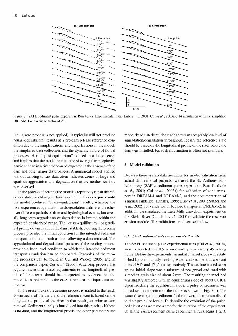
Figure 7 SAFL sediment pulse experiment Run 4b. (a) Experimental data (Lisle et al., 2001, Cui et al., 2003a); (b) simulation with the simplifiedDREAM-1 and a fudge factor of 2.2.

(i.e., a zero process is not applied), it typically will not produce“quasi-equilibrium” results at a pre-dam release reference con-dition due to the simplifications and imperfections in the model,the simplified data collection, and the dynamic nature of fluvialprocesses. Here “quasi-equilibrium” is used in a loose sense,and implies that the model predicts the slow, regular morphody-namic change in a river that can be expected in the absence of thedam and other major disturbances. A numerical model appliedwithout zeroing to raw data often indicates zones of large andspurious aggradation and degradation that are neither realisticnor observed.

In the process of zeroing the model is repeatedly run at the ref-erence state, modifying certain input parameters as required untilthe model produces “quasi-equilibrium” results, whereby theriver experiences aggradation and degradation at different reachesover different periods of time and hydrological events, but over-all, long-term aggradation or degradation is limited within theexpected or observed range. The “quasi-equilibrium” longitudi-nal profile downstream of the dam established during the zeroingprocess provides the initial condition for the intended sedimenttransport simulation such as one following a dam removal. Theaggradational and degradational patterns of the zeroing processprovide a base level condition to which the intended sedimenttransport simulation can be compared. Examples of the zero-ing processes can be found in Cui and Wilcox (2005) and inthe companion paper, Cui et al. (2006). A zeroing process thatrequires more than minor adjustments to the longitudinal pro-file of the stream should be interpreted as evidence that themodel is inapplicable to the case at hand or the input data arein error.

In the present work the zeroing process is applied to the reachdownstream of the dam, and the reference state is based on thelongitudinal profile of the river in that reach just prior to damremoval. Sediment supply is introduced into this reach as if thereis no dam, and the longitudinal profile and other parameters are

modestly adjusted until the reach shows an acceptably low level ofaggradation/degradation throughout. Ideally the reference stateshould be based on the longitudinal profile of the river before thedam was installed, but such information is often not available.

6 Model validation

Because there are no data available for model validation fromactual dam removal projects, we used the St. Anthony FallsLaboratory (SAFL) sediment pulse experiment Run 4b (Lisleet al., 2001; Cui et al., 2003a) for validation of sand trans-port in DREAM-1 and DREAM-2, and the documentation ofa natural landslide (Hansler, 1999; Lisle et al., 2001; Sutherlandet al., 2002) for validation of bedload transport in DREAM-2. Inaddition, we simulated the Lake Mills drawdown experiment onthe Elwha River (Childers et al., 2000) to validate the reservoirerosion module. The validations are discussed below.

6.1 SAFL sediment pulse experiments Run 4b

The SAFL sediment pulse experimental runs (Cui et al., 2003a)were conducted in a 0.5 m wide and approximately 45 m longflume. Before the experiments, an initial channel slope was estab-lished by continuously feeding water and sediment at constantrates of 9 l/s and 45 g/min, respectively. The sediment used to setup the initial slope was a mixture of pea gravel and sand witha median grain size of about 2 mm. The resulting channel bedwas slightly armored with an equilibrium slope of about 0.0108.Upon reaching the equilibrium slope, a pulse of sediment wasintroduced in a section of the flume as shown in Fig. 7(a). Thewater discharge and sediment feed rate were then reestablishedto their pre-pulse levels. To describe the evolution of the pulse,bed elevations were measured for the duration of the experiment.Of all the SAFL sediment pulse experimental runs, Runs 1, 2, 3,


4a, and 4b, only Runs 4a and 4b introduced a fine sediment pulsewhich can be viewed as the simulation of sand transport over agravel-bedded river. Between Runs 4a and 4b, Run 4a was a trialrun without intensive measurements. The fine sediment (sand)pulse introduced in Runs 4a and 4b had a geometric mean grainsize of approximately 0.55 mm and geometric standard deviationof about 2.31. The experimental results for Run 4b are shown inFig. 7(a).

DREAM-1 was developed to simulate dam removal at fieldscale, and the current model structure do not allow for simula-tion of flume experiments. For example, the output of the modelis given in terms of daily, weekly and monthly results and cannotprovide the fine time scales appropriate for a flume experiment.We therefore developed a simplified flume version of DREAM-1to simulate the SAFL sediment pulse experiment Run 4b. In sim-plifying DREAM-1, a “ fudge factor” was added into the modelto allow the user to adjust the predicted sediment transport rates.For example, a “fudge factor” of 1 means that there is no adjust-ment to the sediment transport rate predicted with Brownlie’s bedmaterial load equation and a factor of 2 means that the sedimenttransport capacity used in the model is twice that predicted byBrownlie’s equation.

The numerical experiments indicated that the simulationunder-predicted the sand transport rate, evidenced by a slowerpulse evolution in the numerical simulation. Increasing the calcu-lated sediment transport rate by a “fudge factor” of 2.2, however,reproduced the experimental results satisfactorily via a visualinspection, as shown in Fig. 7(b). Comparison of Figs 7(a, b)indicates that the adjusted model provided a very accurate repro-duction of the experiment results, including such features as thedispersion and downstream translation of the sediment pulse, thelocations of the leading and trailing edges of the sediment pulse,and the time at which the sediment pulse became so diffuse thatit was difficult to distinguish from the ambient sediment. Notein Fig. 7(b) that the initial bed profile has been smoothed beforeapplying the model.

Wooster (2002) applied the simplified DREAM-1 to simu-late his dam removal experiments and found that a fudge factorof 3.4 produced an excellent match between the simulation andexperimental data.

6.2 Lake Mills drawdown experiment

DREAM-1 was also applied to simulate the Lake Mills draw-down experiment (Childers et al., 2000) in order to validate itsreservoir erosion module. Lake Mills, shown in Fig. 8, is thereservoir behind the Glines Canyon dam on the Elwha Riverunder study for removal (e.g., Bureau of Reclamation, 1996a,b).The Lake Mills drawdown experiment (Childers et al., 2000) wasconducted between April 8 and 26, 1994, when the lake level wasgradually lowered from 179.2 to 173.7 m over a 1-week period,with a lowering rate ranging between 0.3 and 0.9 m/day. Thelake was then held at 173.7 m for a week and then graduallyfilled back to the predrawdown level of 179.2 m (Childers et al.,2000; T. Randle, personal communication). The time variation

Figure 8 Lake Mills, Elwha river showing the monitoring crosssections. Modified from Childers et al. (2000).

173

174

175

176

177

178

179

180

4/8 4/13 4/18 4/23 4/28 5/3 5/8

Time

Wat

er S

urf

ace

Ele

vati

on

in L

ake

Mill

s (m

)

End

of c

ross

sec

tiona

l sur

vey

Figure 9 Lake Mills water surface elevation during the drawdownexperiment; data based on Childers et al. (2000) and T. Randle (personalcommunication).

of lake level in Lake Mills during the drawdown experiment isgiven in Fig. 9.

Note that the Lake Mills drawdown experiment differed fromour assumed dam removal scenario in that the lake drawdownexperiment slowly lowered the lake level as described above andin Childers et al. (2000), while the base level for our assumeddam removal scenario would be lowered instantly. The abovedifference may result in differences in channel erosion patternsand other channel morphology. Despite the differences, the draw-down experiment offered an opportunity to see how the modelresults and field measurements compare at a scale much largerthan a flume.

12 Cui et al.

The current model (DREAM-1) was modified slightly to allowfor the gradual decrease in lake level during the drawdown exper-iment. The input parameters for the simulation are summarizedbelow.

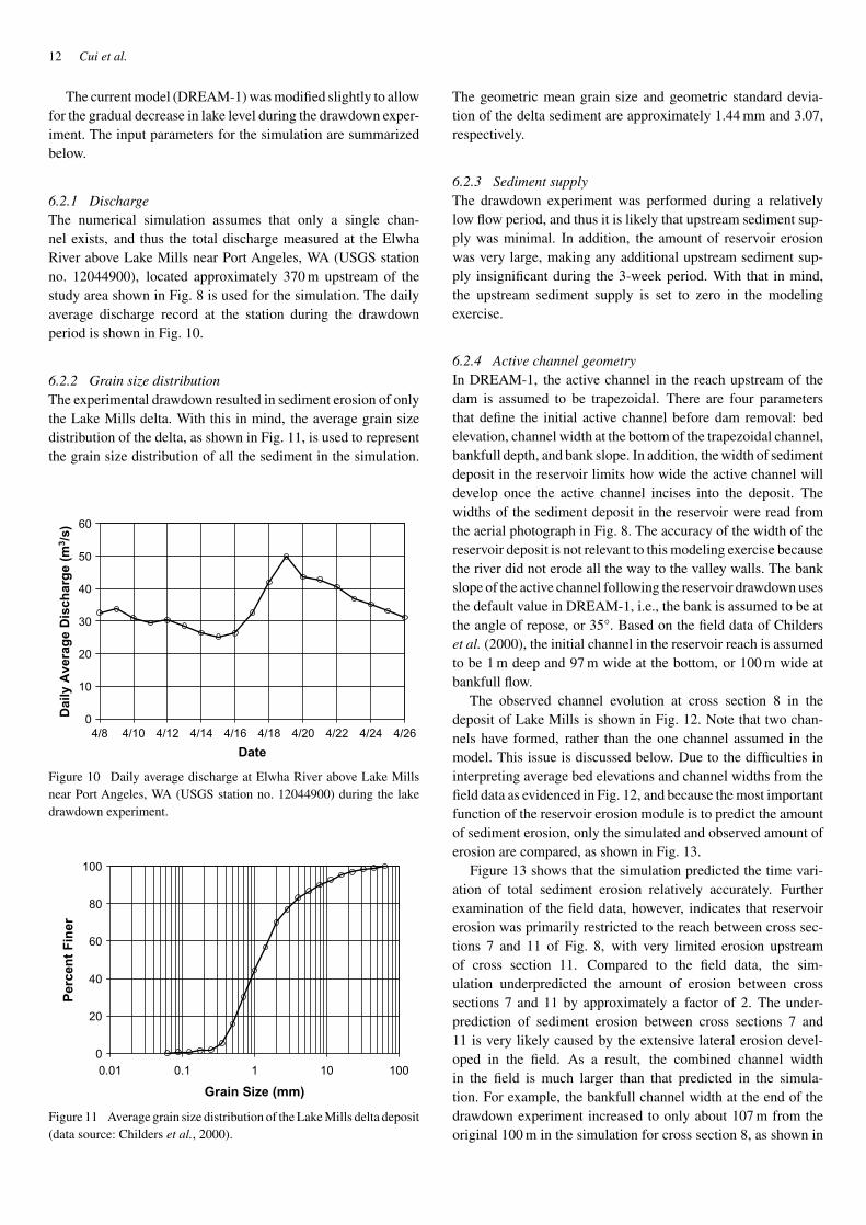
6.2.1 DischargeThe numerical simulation assumes that only a single chan-nel exists, and thus the total discharge measured at the ElwhaRiver above Lake Mills near Port Angeles, WA (USGS stationno. 12044900), located approximately 370 m upstream of thestudy area shown in Fig. 8 is used for the simulation. The dailyaverage discharge record at the station during the drawdownperiod is shown in Fig. 10.

6.2.2 Grain size distributionThe experimental drawdown resulted in sediment erosion of onlythe Lake Mills delta. With this in mind, the average grain sizedistribution of the delta, as shown in Fig. 11, is used to representthe grain size distribution of all the sediment in the simulation.

0

10

20

30

40

50

60

4/8 4/10 4/12 4/14 4/16 4/18 4/20 4/22 4/24 4/26

Date

Dai

ly A

vera

ge

Dis

char

ge

(m3 /

s)

Figure 10 Daily average discharge at Elwha River above Lake Millsnear Port Angeles, WA (USGS station no. 12044900) during the lakedrawdown experiment.

0

20

40

60

80

100

0.01 0.1 1 10 100

Grain Size (mm)

Per

cen

t F

iner

Figure 11 Average grain size distribution of the Lake Mills delta deposit(data source: Childers et al., 2000).

The geometric mean grain size and geometric standard devia-tion of the delta sediment are approximately 1.44 mm and 3.07,respectively.

6.2.3 Sediment supplyThe drawdown experiment was performed during a relativelylow flow period, and thus it is likely that upstream sediment sup-ply was minimal. In addition, the amount of reservoir erosionwas very large, making any additional upstream sediment sup-ply insignificant during the 3-week period. With that in mind,the upstream sediment supply is set to zero in the modelingexercise.

6.2.4 Active channel geometryIn DREAM-1, the active channel in the reach upstream of thedam is assumed to be trapezoidal. There are four parametersthat define the initial active channel before dam removal: bedelevation, channel width at the bottom of the trapezoidal channel,bankfull depth, and bank slope. In addition, the width of sedimentdeposit in the reservoir limits how wide the active channel willdevelop once the active channel incises into the deposit. Thewidths of the sediment deposit in the reservoir were read fromthe aerial photograph in Fig. 8. The accuracy of the width of thereservoir deposit is not relevant to this modeling exercise becausethe river did not erode all the way to the valley walls. The bankslope of the active channel following the reservoir drawdown usesthe default value in DREAM-1, i.e., the bank is assumed to be atthe angle of repose, or 35°. Based on the field data of Childerset al. (2000), the initial channel in the reservoir reach is assumedto be 1 m deep and 97 m wide at the bottom, or 100 m wide atbankfull flow.

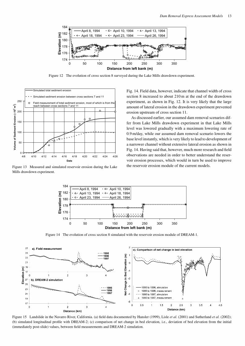
The observed channel evolution at cross section 8 in thedeposit of Lake Mills is shown in Fig. 12. Note that two chan-nels have formed, rather than the one channel assumed in themodel. This issue is discussed below. Due to the difficulties ininterpreting average bed elevations and channel widths from thefield data as evidenced in Fig. 12, and because the most importantfunction of the reservoir erosion module is to predict the amountof sediment erosion, only the simulated and observed amount oferosion are compared, as shown in Fig. 13.

Figure 13 shows that the simulation predicted the time vari-ation of total sediment erosion relatively accurately. Furtherexamination of the field data, however, indicates that reservoirerosion was primarily restricted to the reach between cross sec-tions 7 and 11 of Fig. 8, with very limited erosion upstreamof cross section 11. Compared to the field data, the sim-ulation underpredicted the amount of erosion between crosssections 7 and 11 by approximately a factor of 2. The under-prediction of sediment erosion between cross sections 7 and11 is very likely caused by the extensive lateral erosion devel-oped in the field. As a result, the combined channel widthin the field is much larger than that predicted in the simula-tion. For example, the bankfull channel width at the end of thedrawdown experiment increased to only about 107 m from theoriginal 100 m in the simulation for cross section 8, as shown in


174

176

178

180

182

184

0 50 100 150 200 250 300 350

Distance from left bank (m)

Ele

vati

on

(m

) April 8, 1994 April 10, 1994 April 13, 1994

April 18, 1994 April 23, 1994 April 26, 1994

Figure 12 The evolution of cross section 8 surveyed during the Lake Mills drawdown experiment.

0

50

100

150

200

250

4/8 4/10 4/12 4/14 4/16 4/18 4/20 4/22 4/24 4/26

Date

Vo

lum

e o

f S

edim

ent

Ero

sio

n (

×103 m

3 )

Simulated total sediment erosion

Simulated sediment erosion between cross sections 7 and 11

Field measurement of total sediment erosion, most of which is from thereach between cross sections 7 and 11

Figure 13 Measured and simulated reservoir erosion during the LakeMills drawdown experiment.

174

176

178

180

182

184

0 50 100 150 200 250 300 350Distance from left bank (m)

Ele

vati

on

(m

) April 8, 1994 April 10, 1994April 13, 1994 April 18, 1994April 23, 1994 April 26, 1994

Figure 14 The evolution of cross section 8 simulated with the reservoir erosion module of DREAM-1.

Figure 15 Landslide in the Navarro River, California. (a) field data documented by Hansler (1999), Lisle et al. (2001) and Sutherland et al. (2002);(b) simulated longitudinal profile with DREAM-2; (c) comparison of net change in bed elevation, i.e., deviation of bed elevation from the initial(immediately post-slide) values, between field measurements and DREAM-2 simulation.

Fig. 14. Field data, however, indicate that channel width of crosssection 8 increased to about 210 m at the end of the drawdownexperiment, as shown in Fig. 12. It is very likely that the largeamount of lateral erosion in the drawdown experiment preventederosion upstream of cross section 11.

As discussed earlier, our assumed dam removal scenarios dif-fer from Lake Mills drawdown experiment in that Lake Millslevel was lowered gradually with a maximum lowering rate of0.9 m/day, while our assumed dam removal scenario lowers thebase level instantly, which is very likely to lead to development ofa narrower channel without extensive lateral erosion as shown inFig. 14. Having said that, however, much more research and fieldobservations are needed in order to better understand the reser-voir erosion processes, which would in turn be used to improvethe reservoir erosion module of the current models.

14 Cui et al.

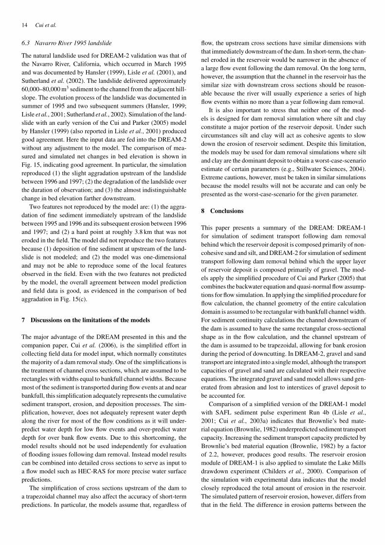
6.3 Navarro River 1995 landslide

The natural landslide used for DREAM-2 validation was that ofthe Navarro River, California, which occurred in March 1995and was documented by Hansler (1999), Lisle et al. (2001), andSutherland et al. (2002). The landslide delivered approximately60,000–80,000 m3 sediment to the channel from the adjacent hill-slope. The evolution process of the landslide was documented insummer of 1995 and two subsequent summers (Hansler, 1999;Lisle et al., 2001; Sutherland et al., 2002). Simulation of the land-slide with an early version of the Cui and Parker (2005) modelby Hansler (1999) (also reported in Lisle et al., 2001) producedgood agreement. Here the input data are fed into the DREAM-2without any adjustment to the model. The comparison of mea-sured and simulated net changes in bed elevation is shown inFig. 15, indicating good agreement. In particular, the simulationreproduced (1) the slight aggradation upstream of the landslidebetween 1996 and 1997; (2) the degradation of the landslide overthe duration of observation; and (3) the almost indistinguishablechange in bed elevation farther downstream.

Two features not reproduced by the model are: (1) the aggra-dation of fine sediment immediately upstream of the landslidebetween 1995 and 1996 and its subsequent erosion between 1996and 1997; and (2) a hard point at roughly 3.8 km that was noteroded in the field. The model did not reproduce the two featuresbecause (1) deposition of fine sediment at upstream of the land-slide is not modeled; and (2) the model was one-dimensionaland may not be able to reproduce some of the local featuresobserved in the field. Even with the two features not predictedby the model, the overall agreement between model predictionand field data is good, as evidenced in the comparison of bedaggradation in Fig. 15(c).

7 Discussions on the limitations of the models

The major advantage of the DREAM presented in this and thecompanion paper, Cui et al. (2006), is the simplified effort incollecting field data for model input, which normally constitutesthe majority of a dam removal study. One of the simplifications isthe treatment of channel cross sections, which are assumed to berectangles with widths equal to bankfull channel widths. Becausemost of the sediment is transported during flow events at and nearbankfull, this simplification adequately represents the cumulativesediment transport, erosion, and deposition processes. The sim-plification, however, does not adequately represent water depthalong the river for most of the flow conditions as it will under-predict water depth for low flow events and over-predict waterdepth for over bank flow events. Due to this shortcoming, themodel results should not be used independently for evaluationof flooding issues following dam removal. Instead model resultscan be combined into detailed cross sections to serve as input toa flow model such as HEC-RAS for more precise water surfacepredictions.

The simplification of cross sections upstream of the dam toa trapezoidal channel may also affect the accuracy of short-termpredictions. In particular, the models assume that, regardless of

flow, the upstream cross sections have similar dimensions withthat immediately downstream of the dam. In short-term, the chan-nel eroded in the reservoir would be narrower in the absence ofa large flow event following the dam removal. On the long term,however, the assumption that the channel in the reservoir has thesimilar size with downstream cross sections should be reason-able because the river will usually experience a series of highflow events within no more than a year following dam removal.

It is also important to stress that neither one of the mod-els is designed for dam removal simulation where silt and clayconstitute a major portion of the reservoir deposit. Under suchcircumstances silt and clay will act as cohesive agents to slowdown the erosion of reservoir sediment. Despite this limitation,the models may be used for dam removal simulations where siltand clay are the dominant deposit to obtain a worst-case-scenarioestimate of certain parameters (e.g., Stillwater Sciences, 2004).Extreme cautions, however, must be taken in similar simulationsbecause the model results will not be accurate and can only bepresented as the worst-case-scenario for the given parameter.

8 Conclusions

This paper presents a summary of the DREAM: DREAM-1for simulation of sediment transport following dam removalbehind which the reservoir deposit is composed primarily of non-cohesive sand and silt, and DREAM-2 for simulation of sedimenttransport following dam removal behind which the upper layerof reservoir deposit is composed primarily of gravel. The mod-els apply the simplified procedure of Cui and Parker (2005) thatcombines the backwater equation and quasi-normal flow assump-tions for flow simulation. In applying the simplified procedure forflow calculation, the channel geometry of the entire calculationdomain is assumed to be rectangular with bankfull channel width.For sediment continuity calculations the channel downstream ofthe dam is assumed to have the same rectangular cross-sectionalshape as in the flow calculation, and the channel upstream ofthe dam is assumed to be trapezoidal, allowing for bank erosionduring the period of downcutting. In DREAM-2, gravel and sandtransport are integrated into a single model, although the transportcapacities of gravel and sand are calculated with their respectiveequations. The integrated gravel and sand model allows sand gen-erated from abrasion and lost to interstices of gravel deposit tobe accounted for.

Comparison of a simplified version of the DREAM-1 modelwith SAFL sediment pulse experiment Run 4b (Lisle et al.,2001; Cui et al., 2003a) indicates that Brownlie’s bed mate-rial equation (Brownlie, 1982) underpredicted sediment transportcapacity. Increasing the sediment transport capacity predicted byBrownlie’s bed material equation (Brownlie, 1982) by a factorof 2.2, however, produces good results. The reservoir erosionmodule of DREAM-1 is also applied to simulate the Lake Millsdrawdown experiment (Childers et al., 2000). Comparison ofthe simulation with experimental data indicates that the modelclosely reproduced the total amount of erosion in the reservoir.The simulated pattern of reservoir erosion, however, differs fromthat in the field. The difference in erosion patterns between the


simulation and the field experiment is, however, very likelycaused by the extensive lateral erosion in the field induced bythe slowly lowered lake level. DREAM-2 is validated with datafor a natural landslide on the Navarro River, California, docu-mented by Hansler (1999), Lisle et al. (2001) and Sutherlandet al. (2002), with good agreement between simulation and fielddata.

The companion paper, Cui et al. (2006) provides a series ofsample runs as sensitivity tests pertaining to some of the importantuser-defined and fixed parameters.

Acknowledgments

Model development was partially supported by National Oceanicand Atmospheric Administration (NOAA). Funding to StillwaterSciences, the University of Minnesota and University of Califor-nia, Berkeley that directly or indirectly benefited the developmentof the current models was provided by the following sources:Portland General Electric (PGE), PacifiCorp, National ScienceFoundation (NSF), Environmental Protection Agency (EPA),National Aviation and Space Administration (NASA), Ok TediMining Limited (OTML) and the St. Johns River Water Manage-ment District, Florida. We thank Drs. Marcelo Garcia (U Illinois),Thomas Lisle (USFS), James Pizzuto (U Delaware) and StephenWiele (USGS), whose reviews to the Marmot Dam removal mod-eling sparked many improvements in the development of thecurrent models. Many Stillwater employees contributed to thedevelopment of the models: Andrew Wilcox (now with ColoradoState University), Frank Ligon, Jennifer Vick (now with McBainand Trush), John O’Brien (now with US Forest Service) andBruce Orr. Peter Downs reviewed an earlier draft and pro-vided many useful suggestions. This paper is a contribution ofthe National Center for Earth-surface Dynamics (NCED) basedat St. Anthony Falls Laboratory, University of Minnesota, inwhich the University of California, Berkeley participates, andof which Stillwater Sciences, Berkeley, California is a partner.The useful suggestions from two anonymous reviewers have beenincorporated into the manuscript.

Notation

B = Bankfull channel widthB̄ = Average bankfull width for the reach close to and

downstream of the damBb = Bottom width of the trapezoidal channelBm = Minimum bottom width of the trapezoidal channelBt = Top width of the trapezoidal channelD = Particle grain sizeD̄j = Geometric mean grain size of the jth size groupDsg = Geometric mean grain size of surface gravelfbj = Volumetric fraction of the jth size group in subsur-

face gravelfg = Fraction of gravel in sediment depositfIj = Volumetric fraction of the jth size group in the

gravel that is exchanged between bedload andchannel in a gravel-bedded river

fsa = Fraction of sand in sediment depositF = Froude numberFj = Volumetric fraction of the jth size group in

surface gravel of a gravel-bedded riverF ′j = Fraction of the area for the jth gravel size group

exposed to the flow in surface layerg = Acceleration of gravityh = Water depthHd = Depth of the trapezoidal channelH̄d = Average bankfull depth for the reach close to and

downstream of the damks = Roughness heightLa = Active layer (surface layer) thicknesspj = Volumetric fraction of the jth gravel size group

in bedload of a gravel-bedded riverqgl, qsl = Lateral gravel and sand supply to the channel, in

volume per unit channel length per unit timeQg = Volumetric transport rate of gravelQ̄g = Long-term average volumetric rate of gravel

supplyQg0 = Volumetric rate of gravel supplyQs = Volumetric transport rate of sandQ̄s = Long-term average volumetric rate of sand

supplyQs0 = Volumetric rate of sand supplyQw = Water discharge

Q̄wash = Long-term average volumetric rate of wash loadsupply

Qwash0 = Volumetric rate of wash load supplyS0 = Channel bed slopeSf = Friction slopet = Timeu∗ = Shear velocityvs = Sediment particle settling velocityx = Downstream distance

α0, α1, α2 = Coefficients for proportioning sediment supplyβ = Volumetric abrasion coefficientφ = Grain size φ-scaleηb = Non-erodible base (bedrock) elevationηg = Thickness of gravel depositηs = Thickness of sand depositκ = von Karman costantλp = Porosity of the sediment depositθ = Bank angle of the trapezoidal channel, which is

assumed to be the angle of reposeσsg = Geometric standard deviation of surface gravelψ = Grain size ψ-scale, which is the negative of ψ-

scale.

References

1. ASCE (1997). Guidelines for Retirement of Dams andHydroelectric Facilities. ASCE, New York, NY, 222 pp.

2. Bhallamudi, S.M. and Chaudhry, M.H. (1991). “Numer-ical Modeling of Aggradation and Degradation in AlluvialChannels”. J. Hydraul. Engng., ASCE 117(9), 1145–1164.

16 Cui et al.

3. Brownlie, W.R. (1982), “Prediction of Flow Depth andSediment Discharge in Open Channels”. PhD Thesis,California Institute of Technology, Pasadena, CA.

4. Bureau of Reclamation (1996a). Removal of Elwha andGlines Canyon Dams. Elwha River Ecosystem and FisheriesRestoration Project, Washington, Elwha Technical SeriesPN-95-7, May.

5. Bureau of Reclamation (1996b). Sediment Analysis andModeling of the River Erosion Alternative. Elwha RiverEcosystem and Fisheries Restoration Project, Washington,Elwha Technical Series PN-95-9, October.

6. Childers, D., Kresch, D.L., Gustafson, S.A.,Randle, T.J., Melena, J.T. and Cluer, B. (2000). “Hydro-logic Data Collected during the 1994 Lake Mills DrawdownExperiment, Elwha River, Washington”. U.S. Geologi-cal Survey Water-Resources Investigations Report 99–4215,Tacoma, Washington.

7. Cui,Y. and Parker, G. (1997). “A Quasi-normal SimulationofAggradation and Downstream Fining with Shock Fitting”.Int. J. Sed. Res. 12(2), 68–82.

8. Cui,Y. and Parker, G. (1998). “The Arrested Gravel Front:Stable Gravel-Sand Transitions in Rivers. Part II: GeneralNumerical Solution”. J. Hydraul. Res. 36(2), 159–182.

9. Cui, Y. and Parker, G. (2005). “Numerical Model of Sedi-ment Pulses and Sediment Supply Disturbances in MountainRivers”. J. Hydraul. Engng. 131(8).

10. Cui, Y. and Wilcox, A. (2005). “Development and Appli-cation of Numerical Modeling of Sediment Transport Asso-ciated with Dam Removal”. In: Garcia, M.H. (ed.), Sed-imentation Engineering, ASCE Manual 54, Vol. 2, ASCE,Reston, Va.

11. Cui, Y., Parker, G. and Paola, C. (1996). “Numeri-cal Simulation of Aggradation and Downstream Fining”.J. Hydraul. Res. 34(2), 184–204.

12. Cui, Y., Parker, G., Lisle, T.E., Gott, J.,Hansler, M.E., Pizzuto, J.E., Allmendinger, N.E. andReed, J.M. (2003a). “Sediment Pulses in Mountain Rivers.Part 1. Experiments”. Water Resour. Res. 39(9), 1239,doi: 10.1029/2002WR001803.

13. Cui, Y., Parker, G., Pizzuto, J.E. and Lisle, T.E. (2003b).“Sediment Pulses in Mountain Rivers. Part 2. Comparisonbetween Experiments and Numerical Predictions”. WaterResour. Res. 39(9), 1240, doi: 10.1029/2002WR001805.

14. Cui, Y., Parker, G., Braudrick, C., Dietrich, W.E. andCluer, B. (2006). “Dam Removal Express AssessmentModels (DREAM). Part 2: Sample Runs/Sensitivity Tests”.J. Hydraul. Res. (this volume).

15. Dietrich, W.E. (1982). “Settling Velocities of NaturalParticles”. Water Resour. Res. 18(6), 1615–1626.

16. Hansler, M.E. (1999). “Sediment Wave Evolution andAnalysis of a One-dimensional Sediment Routing Model,Navarro River, Northwestern California”. A thesis presentedto The Faculty of Humboldt State University in partial ful-fillment of the requirements for the degree of Master ofSciences, December, 128 pp.

17. Hoey, T.B. and Ferguson, R.I. (1994). “Numerical Simula-tion of Downstream Fining by Selective Transport in GravelBed Rivers: Model Development and Illustration”. WaterResour. Res. 30, 2251–2260.

18. Holly, F.M. and Rahuel, J.L. (1990a). “New Numeri-cal/Physical Framework for Mobile-bed Modeling. Part I:Numerical and Physical Principles”. J. Hydraul. Res. IAHR28(4), 401–416.

19. Holly, F.M. and Rahuel, J.L. (1990b). “New Numeri-cal/Physical Framework for Mobile-bed Modeling. Part II:Test Applications”. J. Hydraul. Res. IAHR 28(5), 545–564.

20. Li, R.M., Mussetter, R.A. and Grindeland, T.R. (1988).“Sediment-routing Model: HEC2SR”. Report Presentedto Subcommittee on Sedimentation, Interagency AdvisoryCommittee on Water Data.

21. Lisle, T.E., Cui, Y., Parker, G., Pizzuto, J.E. andDodd, A.M. (2001). “The Dominance of Dispersion in theEvolution of Bed Material Waves in Gravel-Bed Rivers”.Earth Surface Processes Landforms 26, 1409–1420.

22. Paola, C., Parker, G., Seal, R., Sinha, S.K.,Southard, J.B. and Wilcock, P.R. (1992). “DownstreamFining by Selective Deposition in a Laboratory Flume”.Science 258, 1757–1760.

23. Parker, G. (1990a). “Surface-based Bedload TransportRelation for Gravel Rivers”. J. Hydraul. Res. 28(4),417–436.

24. Parker, G. (1990b). “The ACRONYM Series of pascalPrograms for Computing Bedload Transport in GravelRivers”. External Memorandum M-220, St. Anthony FallsLaboratory, University of Minnesota, 124 pp.

25. Parker, G. (1991a). “Selective Sorting and Abrasion ofRiver Gravel. I: Theory”. J. Hydraul. Engng. 117(2),131–149.

26. Parker, G. (1991b). “Selective Sorting and Abrasion ofRiver Gravel. I: Application”. J. Hydraul. Engng. 117(2),150–171.

27. Rahuel, J.L., Holly, F.M., Chollet, J.P., Belleudy, J.P.and Yang, G. (1989). “Modeling of Riverbed Evolutionfor Bedload Sediment Mixtures”. J. Hydraul. Engng. ASCE115(11), 1521–1542.

28. Seal, R., Paola, C., Parker, G., Southard, J. andWilcock, P. (1997). “Experiments on Downstream Finingof Gravel: I. Narrow Channel Runs”. J. Hydraul. Engng.123(10), 874–884.

29. Stillwater Sciences (1999). “Preliminary Modeling ofSand/Silt Release from Soda Springs Reservoir in theEvent of Dam Removal”. Technical Report Prepared forPacifiCorp, June.

30. Stillwater Sciences (2000). “Numerical Modeling of Sedi-ment Transport in the Sandy River, OR Following Removalof Marmot Dam”. Technical Report Prepared for PortlandGeneral Electric, March.

31. Stillwater Sciences (2004). “A Preliminary Evaluation ofthe Potential Downstream Sediment Deposition Follow-ing the Removal of Iron Gate, Copco, and JC Boyle


dams, Klamath River, CA”. Final report prepared forAmerican Rivers, American Trout, Friends of the River,and Trout Unlimited, May. http://www.amrivers.org/doc_repository/DamRemoval/StillwaterFinalReport-full.pdf, accessed in January 2005.

32. Sutherland, D.G., Hansler-Ball, M., Hilton, S.J. andLisle, T.E. (2002). “Evolution of a Landslide inducedSediment Wave in the Navarro River, California”. GSA Bull.114(8), 1036–1048.

33. Toro-Escobar, M.E., Parker, G. and Paola, C. (1996).“Transfer Function for the Deposition of Poorly SortedGravel in Response to Streambed Aggradation”. J. Hydraul.Res. 34(1), 35–54.

34. US Army Corps of Engineers (1993). HEC-6: Scourand Deposition in Rivers and Reservoirs. User’s Man-ual, Hydrologic Engineering Center, US Army Corps ofEngineers.

35. van Rijn, L.C. (1984). “Sediment Transport, Part II: Sus-pended Load Transport”. J. Hydraul. Engng. 110(11),1613–1641.

36. Wilcock, P.R. (1997). A Method for Predicting SedimentTransport in Gravel-Bed Rivers, Department of Geographyand Environmental Engineering, The Johns Hopkins Uni-versity, Baltimore, Maryland 21218, 44 pages, 1 table and13 figures, March 31.

37. Wilcock, P.R. (1998). “Two-fraction Model of InitialSediment Motion in Gravel-Bed Rivers”. Science 280,410–412.

38. Wilcock, P.R. and Crowe, J.C. (2003). “A Surface-basedTransport Model for Sand and Gravel”. J. Hydraul. Engng.129(2), 120–128.

39. Wooster, J. (2002). “Geomorphic Responses FollowingDam Removal: A Flume Study”. Master’s Thesis, GeologyDepartment, University of California, Davis, CA.

Documents

Dam Removal Express Assessment Models (DREAM). Part 1: Model