Embed Size (px)
Citation preview

Computer Simulation and Life Cycle Analysis of a Seasonal Thermal Storage System in a
Residential Building
Alexandre Hugo
A Thesis
in
the Department
of
Building, Civil & Environmental Engineering
Presented in the Partial Fulfillment
for the Degree of Master of Applied Science at
Concordia University
Montreal, Quebec, Canada
November 2008
© Alexandre Hugo, 2008

1*1 Library and Archives Canada
Published Heritage Branch
395 Wellington Street Ottawa ON K1A0N4 Canada
Bibliotheque et Archives Canada
Direction du Patrimoine de I'edition
395, rue Wellington Ottawa ON K1A0N4 Canada
Your file Votre reference ISBN: 978-0-494-45464-0 Our file Notre reference ISBN: 978-0-494-45464-0
NOTICE: The author has granted a nonexclusive license allowing Library and Archives Canada to reproduce, publish, archive, preserve, conserve, communicate to the public by telecommunication or on the Internet, loan, distribute and sell theses worldwide, for commercial or noncommercial purposes, in microform, paper, electronic and/or any other formats.
AVIS: L'auteur a accorde une licence non exclusive permettant a la Bibliotheque et Archives Canada de reproduire, publier, archiver, sauvegarder, conserver, transmettre au public par telecommunication ou par Plntemet, prefer, distribuer et vendre des theses partout dans le monde, a des fins commerciales ou autres, sur support microforme, papier, electronique et/ou autres formats.
The author retains copyright ownership and moral rights in this thesis. Neither the thesis nor substantial extracts from it may be printed or otherwise reproduced without the author's permission.
L'auteur conserve la propriete du droit d'auteur et des droits moraux qui protege cette these. Ni la these ni des extraits substantiels de celle-ci ne doivent etre imprimes ou autrement reproduits sans son autorisation.
In compliance with the Canadian Privacy Act some supporting forms may have been removed from this thesis.
Conformement a la loi canadienne sur la protection de la vie privee, quelques formulaires secondaires ont ete enleves de cette these.
While these forms may be included in the document page count, their removal does not represent any loss of content from the thesis.
Canada
Bien que ces formulaires aient inclus dans la pagination, il n'y aura aucun contenu manquant.

ABSTRACT
Computer Simulation and Life Cycle Analysis of a Seasonal
Thermal Storage System in a Residential Building
Alexandre Hugo
The residential sector represents 17% of Canada's secondary energy use, with more than
78% of this contribution due to space and domestic hot water heating. In that perspective,
systems that do not require any auxiliary energy are of a certain interest. Such objective is
not easy to accomplish, especially in cold climates, but yet can be reached by both upgrading
the buildings overall thermal performance and using efficient renewable energy sources.
An integrated building model is developed into the TRNSYS 16 simulation environment.
First, a typical one-storey detached house, located in Montreal is considered as a base case.
Conventional electric baseboard heaters and an electric domestic hot water storage tank
provide the space heating and domestic hot water requirements. A life cycle performance
of the house is performed and results of the life cycle energy use, environmental impacts
and life cycle cost are presented.
Second, several design alternatives are proposed to improve the life cycle performance of
the base case house. The solution that minimizes the energy demand is finally chosen as a
reference building for the study of long-term thermal storage.
Third, the computer simulation of a solar heating system with solar thermal collectors and
long-term thermal storage capacity is presented. The system is designed to supply hot water
for the radiant floor heating system and domestic hot water. Simulation results show that
the system is able to cover a whole year of energy requirements using a minimum of auxiliary
iii

energy. A sensitivity analysis is performed to improve the overall performance. The life
cycle energy use and life cycle cost of the system are investigated and results presented in
the thesis.
IV

Acknowledgments
I want to express my gratitude to my research supervisors. First, thanks to Dr. Zmeureanu
for his great availability, support and always constructive remarks. His enthusiasm and
thoroughness in research motivated me to strive for the best and will remain forever an
extremely enriching experience. Second, thanks to Dr. Hugues Rivard, Professor at ETS
in the Department of Construction Engineering, Chair of Canada Research in Computer-
Assisted Engineering for Sustainable Building Design for his comments and suggestions
I would like to thank as well the Building Engineering team for creating a pleasant work
environment and for providing me with help whenever I needed it. Particularly, I would
like to acknowledge Mitchell Leckner for his insightful remarks and his ability to bring new
ideas.
During these two demanding years of study, the support of my family and my girlfriend was
extremely important. I would like to thank them for their continuous encouragement.
Finally, I would like to thank the members of my defense committee for their insightful
comments and suggestions, all of whom made valuable contributions to this thesis.
v

This thesis is dedicated to my grandmother for her unconditional love and support.
VI

Table of Contents
List of Figures xi
List of Tables xiii
Nomenclature xv
1 Introduction 1
1.1 Background 1
1.2 Research objectives 3
1.3 Methodology 4
2 Literature review 6
2.1 Net-zero energy homes 6
2.2 International projects and initiatives 7
2.2.1 European Passive House 7
2.2.2 IEA SHC tasks 8
2.2.3 BedZED k Eco-Village development 13
2.3 Canadian initiatives 14
2.3.1 Advanced House program 14
2.3.2 Net-Zero Energy Coalition 17
2.3.3 Solar Building Research Network 17
2.3.4 EQuilibrium Housing 18
2.4 Successful strategies 18
2.5 Solar water heating systems 19
2.5.1 Situation of the solar thermal market 20
2.5.2 Energy storage 23
2.5.3 Seasonal storage 24
2.5.4 Stratification in storage tanks 25
2.6 Solar combisystems 26
2.6.1 Task 26: Solar Combisytems 27
2.6.2 ALTENER 29
2.7 Conclusions 29
vn

3 Life cycle performance of a base case house 31
3.1 Description of the base case house 31
3.2 Description of TRNSYS components used for modelling 34
3.2.1 Type 56: Building envelope 35
3.2.2 Weather input data 37
3.2.3 Type 701: Basement conduction 40
3.2.4 Space heating 43
3.2.5 Occupancy 44
3.2.6 Infiltration 44
3.2.7 Space ventilation 44
3.2.8 Space cooling 46
3.2.9 Humidiflcation 47
3.2.10 Shading devices and artificial lighting 47
3.2.11 Internal heat gains 49
3.2.12 Domestic hot water supply 50
3.3 Energy performance results and discussion 53
3.4 Life cycle analysis of the base case house 59
3.4.1 Life cycle energy use 59
3.4.2 Life cycle emissions 62
3.4.3 Life cycle cost 64
3.4.4 Summary of the results 66
3.5 Life cycle analysis of design alternatives 66
3.5.1 Improvement of the thermal resistance of the building envelope . . . 67
4 Modell ing of a seasonal thermal storage 74
4.1 General description of the system 74
4.2 Heat management approach 76
4.2.1 Solar loop 76
4.2.2 Space heating 76
4.2.3 Domestic hot water 77
4.2.4 Auxiliary heating 77
4.3 Description of TRNSYS components used for modelling 78
4.3.1 Solar loop 79
4.3.2 Space heating 95
4.3.3 Domestic hot water 100
4.4 Preliminary design method 102
4.4.1 System description and simulation model 103
4.4.2 Methodology 106
vm

4.4.3 Input data 108
4.4.4 Results 108
4.5 TRNSYS simulation results and discussion 109
4.5.1 Overall performance 110
4.5.2 Performance of the solar combisystem 115
4.5.3 Collection efficiency 123
4.5.4 Solar fraction 124
4.5.5 Coefficient of performance 124
4.6 Sensitivity analysis 126
4.6.1 Evacuated tube collectors 126
4.6.2 Flat-plate collectors 132
4.6.3 Solutions proposed 138
5 Life cycle performance of the seasonal storage sys tem 139
5.1 Life cycle cost 139
5.1.1 Initial cost 139
5.1.2 Operating cost 141
5.1.3 Simple payback 141
5.1.4 Improved payback 142
5.1.5 Discussion 146
5.2 Life cycle energy use 147
5.2.1 Embodied energy 147
5.2.2 Operating energy use 149
5.2.3 Energy payback time 150
5.2.4 Energy yield ratio 151
5.2.5 Discussion 152
6 Conclusions, contributions and future work 153
6.1 Conclusions 153
6.2 Research contributions 154
6.3 Recommendations for future work 155
References 157
Appendices 170
Appendix A Technical specifications of the HRV system 170
Appendix B Coefficients used to calculate the temperature of cold water from
the city line 171
Appendix C Technical specifications of evacuated tube collectors 172
IX

Appendix D Parameters used in the mathematical models of aqueous solutions of polypropylene glycol 173
Appendix E Technical specifications of flat-plate collectors 174
x

List of Figures
1.1 Greenhouse gas emissions in Canada from 1990 to 2005 and Kyoto target . 2
2.1 Zero-Heating Energy House, Berlin, Germany 11
2.2 Stratifying device for hot water stores 26
3.1 Base case house floors plans 32
3.2 Base case house facades plans 33
3.3 Weather data components 38
3.4 Ground reflectance components 39
3.5 Representation of basement walls, with near and far-field 41
3.6 Connections between Types 56 and 701 42
3.7 Heating system components 44
3.8 Ventilation system components 45
3.9 Combination of ventilation and cooling system components 47
3.10 Relative humidity control components 48
3.11 Shading devices and lighting components 49
3.12 Sequence of the DHW profile in January 51
3.13 Temperature of cold water from the city line 52
3.14 Domestic hot water components 53
3.15 Annual distribution of energy use 54
3.16 Energy signature of the base case house 55
3.17 Representation of interior conditions in the base case house from February 1
to February 4 57
3.18 Representation of interior conditions in the base case house from July 1 to
July 4 58
4.1 Modelling of the system 75
4.2 TRNSYS components used to model the solar loop 79
4.3 Evacuated tube collector 80
4.4 Incidence angle modifiers based on SRCC test results 82
4.5 Solar collector efficiency 83
4.6 Variation of density of propylene glycol with temperature 87
XI
4.7 Variation of specific heat of propylene glycol with temperature 87
4.8 Variation of thermal conductivity of propylene glycol with temperature . . 88
4.9 Variation of dynamic viscosity of propylene glycol with temperature . . . . 88
4.10 Inlets and outlets locations in the seasonal storage tank 91
4.11 Electric power of Solar pump n°l as a function of the control signal . . . . 93
4.12 TRNSYS components used to model the heating loop 96
4.13 Supply temperature as a function of outdoor temperature 97
4.14 TRNSYS components used to model the DHW loop 100
4.15 Schematic of a closed-loop space heating system 103
4.16 Solar fraction as a function of the storage volume 109
4.17 Comparison between the base case and the solar combisystem I l l
4.18 Annual distribution of electricity use 112
4.19 Monthly average of operative temperature 113
4.20 Operative temperature in February 114
4.21 Horizontal solar radiation and outdoor temperature 114
4.22 Inside surface temperature on the first floor 115
4.23 Temperatures in the storage tank during the first year of operation 117
4.24 Temperatures in the storage tank during the second year of operation . . . 117
4.25 Monthly average water temperature in the storage tank 118
4.26 Solar pump n°2 mass flow rates 120
4.27 Mass flow rates of the pump used for space heating 120
4.28 Mass flow rates of the pump used for space DHW 121
4.29 Monthly outlet collectors temperature 122
4.30 Variation of the storage tank temperature with the tilt angle during the
month of January 131
4.31 Variation of rjxH+ELEC a n d the COP with the tilt angle 131
4.32 Solar collector efficiency 133
4.33 Variation of the storage tank temperature with the tilt angle during the
month of February 137
4.34 Variation of TJTH+ELEC and the COP with the tilt angle 137
5.1 Cumulative savings of the design alternatives 143
5.2 Impact of the inflation rate of electricity on cumulative savings 144
5.3 Impact of recent economical data and ecoEnergy program on cumulative savingsl45
5.4 Impact of incentives on cumulative savings 146
XII
List of Tables
1.1 Canada's secondary energy use by sector and residential secondary energy
consumption by end-use, 2005 3
2.1 Monitoring results of BedZED & Eco-Village Development 14
2.2 Overview of the Advanced Houses program 16
2.3 Average energy reduction based on different strategies 20
2.4 Market development of flat-plate and evacuated tubular collectors in some
countries; installed capacity per year from 1999 until 2006, total capacity in
operation in 2006 (absolute and per inhabitant) and the corresponding heat
production and CO2 reduction per year 22
2.5 Distribution of different solar collector by country in operation at the end of
2006 23
2.6 Distribution of different applications by country for the total capacity of
flat-plate and evacuated tube collectors in operation at the end of 2006 . . . 27
3.1 List of TRNSYS types 34
3.2 Base case house characteristics 37
3.3 Monthly ground reflectance values 39
3.4 Parameters for the basement conduction model 40
3.6 Monthly repartition and distribution of energy use 54
3.8 Distribution of embodied energy per envelope component 61
3.9 Annual average electricity mix in Quebec and power plants energy efficiencies 61
3.10 Distribution of embodied emissions per envelope component 62
3.13 Life cycle profile of the base case house 66
3.14 Comparison between typical insulation materials 67
3.15 Summary of building envelope's thermal characteristics for each design
alternatives 69
3.16 Insulation materials used in design alternatives 70
3.17 Summary of performance of proposed design alternatives 71
3.18 Reduction of embodied energy use, emissions of greenhouse gases and initial
costs compared with the base case house 72
xm

3.19 Reduction of annual energy use, emissions of greenhouse gases and operating
costs compared with the base case house 72
3.20 Reduction of life cycle energy use, emissions, and cost for the different design
alternatives compared with the base case house 73
4.1 List of TRNSYS types used for modelling the seasonal storage system . . . 78
4.3 Solar collector technical data 81
4.6 Thermophysical properties of glycol used in the study 89
4.7 Recommended dimensions of pipes 90
4.21 Parameters used in the preliminary design method 108
4.22 Monthly repartition and distribution of electricity use 110
4.23 Time of operation and average mass flow rate of pumps 119
4.29 Performance of the solar combisytem for different storage tank volumes . . 127
4.30 Performance of the solar combisytem for different collector areas 127
4.31 Influence of the tank insulation on the performance of the solar combisystem 128
4.32 Performance of the solar combisytem for different values of rhsoiar 129
4.33 Performance of the solar combisytem for different tilt angles 129
4.34 Temperature in the storage tank for different tilt angles 130
4.35 Solar collector technical data 132
4.36 Influence of the tank insulation on the performance of the solar combisystem 134
4.37 Performance of the solar combisytem for different values of thsoiaT . . . . . . 134
4.38 Performance of the solar combisytem for different tilt angles 135
4.39 Temperature in the storage tank for different tilt angles 136
4.40 Proposed design alternatives 138
4.41 Performance of the design alternatives 138
5.1 Initial cost of the solar combisystem 140
5.3 Simple payback of the design alternatives 142
5.5 Improved payback for different economic situations 147
5.6 Embodied energy of flat-plate solar collectors 148
5.7 Total embodied energy of the design alternatives 149
5.9 Energy payback time of the design alternatives 151
xiv

Nomenclature
A Area [m2]
ao Optical efficiency
oi First-order coefficient in collector efficiency equation [W/(m2-K)]
02 Second-order coefficient in collector efficiency equation [W/(m2-K2)]
C Cost [$]
Cp Specific heat [J/(kg-°C)]
caps Thermal capacitance [GJ/°C]
CO2 Equivalent carbon dioxide emissions [kg]
COP Coefficient of performance
E Annual primary energy generated [kWh/yr]
EPT Energy payback time [years]
EYR Energy yield ratio
& Solar fraction
F' Collector efficiency factor
FR Overall collector heat removal efficiency factor
xv

G Solar radiation [W/m2]
hc Convective heat transfer coefficient [W/(m2-°C)]
i Discount rate
i' Effective interest rate
j Inflation rate
JE Inflation rate of electricity
K Incidence angle modifier
L Life span [years]
rh Mass flow rate [kg/s or kg/h]
N Number of days in the month, number of years
Ns Number of identical collectors in series
Nsnow Number of days with snow depth greater than 5 cm
P Electrical power [W]
PW Present Worth [$]
Q Energy [kWh]
v Correction factor
T Temperature [°C]
Tp Freezing temperature [K]
Tdty Temperature of cold water from the city line [°C]
xvi

U Internal energy of storage [GJ]
U'L Modified first-order collector efficiency [W/(m
UA Heat transfer capacity rate [W/°C]
V Volume [m3]
v Wind velocity [m/s]
W Annual energy output [GJ/yr]
Subscripts
aux Auxiliary
c Collector, critical
calc Calculated
combi Combisystem
d Day
db Dry-bulb
DHW Domestic hot water
ELEC Electrical
/ Final
h Hot
HX Heat exchanger
i Inlet, initial
xvii

/ Longitudinal
min Minimum
n Normal
o Out, outdoor, outlet
pp Power plant
R Room
ret Return
set Setpoint
T On a tilted plane
t Tank, transversal
TH Theoretical
u Useful
Greek symbols
a Absorptance, tilt angle [°]
ai_5 Equivalent CO2 emissions due to the generation of electricity [kt C02/TWh]
e Effectiveness
77 Efficiency
7 Control signal
A Thermal conductivity [W/(m.°C)]
xviii

fj, Dynamic viscosity [Pa-s]
p Density [kg/m3]
Pnosnow Snow-free albedo of ground
psnow Snow-covered albedo of ground
r Transmittance
9 Incidence angle [°]
£ Concentration of propylene-glycol
xix

Chapter 1
Introduction
1.1 Background
Climate change is recognized by many scientists as one of the greatest challenges facing
Canada, and the world today. In February 2007, the Intergovernmental Panel on Climate
Change released a report supporting the idea that the global warming is - with 90%
certainty - caused by human activity (IPCC, 2007). The document forecasts that the
average temperature will rise by 1.8 to 4°C by the year 2100 and sea levels will creep up by
17.8 to 58.4 cm by the end of the century. If polar sheets continue to melt, another rise of
9.9 to 19.8 cm is possible.
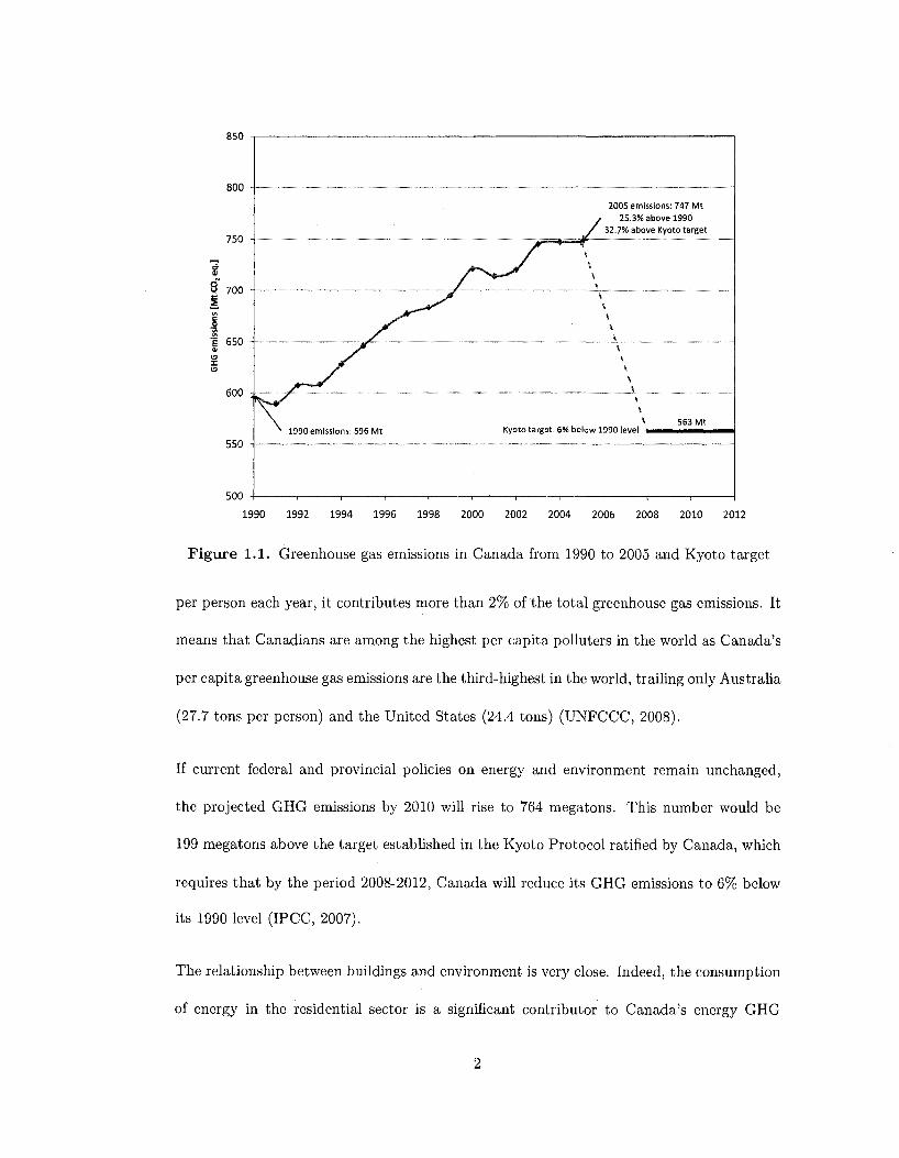
In Canada, greenhouse gas (GHG) emissions have increased by 25% between 1990 and 2005
(Figure 1.1), from 596 megatons to 747 megatons of carbon dioxide equivalent (Mt CO2 eq.),
the standard of measurement for greenhouse gases (IPCC, 2007). This represents the biggest
percentage increase among G8 countries over the same time period, according to a report
published by Statistics Canada (2008). The study says the resulting growth in GHG is in
part attributable to a number of other changes in the country over the same time period,
notably demographic and economic growth.
Canada has about 0.5% of the world's population but, with an average of 23 tons CO2 eq.
1
850
800
550
500
2005 emissions: 747 Mt 25.3% above 1990
32.7% above Kyoto target
1990 emissions'. 596 Mt * 563 Mt
Kyoto target: 6% below 1990 level m > i ^ — ^ _
1990 1992 1994 1996 1998 2000 2002 2004 2006 2008 2010 2012
Figure 1.1. Greenhouse gas emissions in Canada from 1990 to 2005 and Kyoto target
per person each year, it contributes more than 2% of the total greenhouse gas emissions. It
means that Canadians are among the highest per capita polluters in the world as Canada's
per capita greenhouse gas emissions are the third-highest in the world, trailing only Australia
(27.7 tons per person) and the United States (24.4 tons) (UNFCCC, 2008).
If current federal and provincial policies on energy and environment remain unchanged,
the projected GHG emissions by 2010 will rise to 764 megatons. This number would be
199 megatons above the target established in the Kyoto Protocol ratified by Canada, which
requires that by the period 2008-2012, Canada will reduce its GHG emissions to 6% below
its 1990 level (IPCC, 2007).
The relationship between buildings and environment is very close. Indeed, the consumption
of energy in the residential sector is a significant contributor to Canada's energy GHG

emissions since it is responsible of 17% of secondary energy use (Table 1.1). The space and
domestic hot water heating account for 78% of the residential energy use.
Table 1.1. Canada's secondary energy use by sector and residential secondary energy consumption by end-use, 2005. From (NRCan, 2006)
Energy use
Contribution
Energy use
Contribution
[PJ]
[%]
[PJ]
[%]
Industrial
3,209
38
Space heating
846
60
Energy use by sector
Transportation
2,502
30
Residential Commercial
1,402 1,153
17 14
Residential energy consumption by end-use
Water heating
248
18
Appliances Lighting
203 68 14 5
Agriculture
209
2
Space cooling
37
3
Based on these facts, it can be concluded that the construction and operation of buildings
represent a large quantity of energy and create substantial amounts of harmful pollutants
emissions. The way that a building is designed can affect the environment that immediately
surrounds us in a severe way. More globally, the reduction of energy consumption by means
of energy-saving policies, the use renewable energy resources for substitution of fossil energy
sources and the reduction of CO2 emissions will have to become a priority in near future.
1.2 Research objectives
The proposed research aims to explore ways to lower the energy use and greenhouse gases
emissions throughout the life cycle of a typical Canadian house, and evaluate its associated
life cycle cost. The purpose is to analyze some practical and effective solutions to minimize
the life cycle energy use and emissions in a residential building, and eventually to promote
the research results in the engineering and architectural communities.
The focus is made on applications taking full advantage of available renewable energies
3

for space and water heating. More specifically, the system is intended to reduce the
corresponding energy use to a minimum by means of a seasonal storage system.
1.3 Methodology
In order to achieve the stated objectives, the following methodology is proposed:
— A literature survey is conducted to review existing and future projects of low energy
and net-zero houses in different parts of the world and deduce successful strategies,
as well as key factors to design efficient solar thermal systems for space and water
heating;
— Using the simulation program TRNSYS 16, the integrated building model of a single
family house in Montreal is developed;
— The life cycle performance of the base case house is carried out by estimating the life
cycle energy use, life cycle emissions and life cycle cost;
— Several design alternatives that upgrade the life cycle performance of the base case
house are investigated;
— The modelling of a solar combisystem with a long-term thermal storage capacity is
presented;
— A sensitivity analysis, based on a certain set of design parameters, is achieved to
evaluate the repercussions of those parameters on the overall performance of the
system;
— A life cycle analysis is employed to estimate the life cycle cost and life cycle energy
4

use of the system.
5

Chapter 2
Literature review
The literature survey conducted for the purpose of this study aims to review the existing
and future projects of energy efficient houses in different continents of the world. A review
of available and successful technologies is conducted in order to effectively implement the
low energy houses concept under the Canadian cold climate.
This chapter focuses as well on solar applications used to provide space or water heating
commonly named solar "combisystems". The overview on the worldwide situation of the
solar thermal market is given, followed by a summary of some major research results from
the recent years. Finally, based on these studies, efficient methods to design a seasonal
storage system are presented and used as a starting point for this work.
2.1 Net-zero energy homes
As countries are starting to instigate environmental measures to reduce green house gas
emissions to fight global warming, there is an increasing interest in developing strategies
and initiatives that encourage the market introduction of what are called low and net-zero
energy homes (NZEH).
By definition, such home is not only energy efficient as it also produces its own power (Net-
6

Zero Energy Home Coalition, 2007). Just like a typical home, a NZEH is connected to, and
uses energy from, the local electric utility. But unlike typical homes, at times the NZEH
makes enough power to send some back to the utility. Annually, a NZEH produces enough
energy to offset the amount purchased from the utility-resulting in a net-zero annual energy
bill.
2.2 International projects and initiatives
2.2.1 European Passive House
The term "Passive House" is a standard that refers to buildings in which the space heat
requirement is reduced by means of passive measures to the point at which there is no
longer any need for a conventional heating system; the air supply system essentially suffices
to distribute the remaining heat requirement. It is basically a refinement of the low energy
house standard. To permit this, it is crucial that buildings peak heating loads do not
exceed 10 W/m 2 (Schnieders and Hermelink, 2006), which corresponds roughly to average
energy consumptions of 15 kWh/(m2-year) (under Central Europe climatic conditions). In
addition, efficient technologies are also used to decrease the other sources of consumptions,
like electricity for household appliances.
CEPHEUS (Cost Efficient Passive Houses as EUropean Standards) was a project within
the THERMIE-Programme of the European Commission (CEPHEUS, 2007). Started in
1998, this demonstration project served to examine and prove the sustainability of the
Passive House concept in Europe. Fourteen inexpensive Passive Houses with a total of
221 residential units were built in five different countries. All houses have occupants and
7

were evaluated via similar measurement procedures. The target of the CEPHEUS project
was to keep the total primary energy requirement for space heating, domestic hot water
and household appliances below 120 kWh/(m2-year). At this time, this was dividing by a
factor of 2 to 4 the specific consumption levels of new buildings designed to the standards
applicable across Europe (CEPHEUS, 2001). All this had the following goals:
— To demonstrate technical feasibility of achieving the targeted energy performance
indexes at low extra cost for an array of different buildings;
— To give development impulses for the further design of energy- and cost-efficient
buildings and for the further development and accelerated market introduction of
innovative technologies compliant with Passive House standards;
— To facilitate the broad market introduction of cost-efficient Passive Houses.
Measurement data presented by Schnieders and Hermelink indicate average space heating
savings of 80% compared to the reference consumption of conventional new buildings. In
the same way, final and primary energy were reduced by more than 50%. These results show
that the Passive House standard is clearly a great achievement as it enhances the principle
of low energy buildings by fulfilling fully its commitments.
2.2.2 IEA SHC t asks
The International Energy Agency was established in 1974 as an independent agency within
the framework of the Economic Cooperation and Development (OECD) to achieve a
comprehensive program of energy cooperation among its 25 member countries and the
Commission of the European Communities (IEA, 2007). A significant part of the Agency's
program involves collaboration in the research, development and demonstration of new
8
energy technologies to reduce reliance on imported oil, increase long-term energy security
and reduce greenhouse gas emissions of its member's. Research is carried out through
different implementing agreements. The Solar Heating and Cooling (SHC) Program was
one of the first implementing agreements to be established. Since 1977, its 21 members
have been cooperating to develop active solar, passive solar and photovoltaic technologies
and their application in buildings.
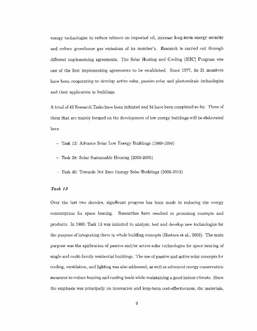
A total of 42 Research Tasks have been initiated and 34 have been completed so far. Three of
them that are mainly focused on the development of low energy buildings will be elaborated
here:
- Task 13: Advance Solar Low Energy Buildings (1989-1994)
- Task 28: Solar Sustainable Housing (2000-2005)
- Task 40: Towards Net Zero Energy Solar Buildings (2008-2013)
Task 13
Over the last two decades, significant progress has been made in reducing the energy
consumption for space heating. Researches have resulted in promising concepts and
products. In 1989, Task 13 was initiated to analyze, test and develop new technologies for
the purpose of integrating them in whole building concepts (Hestnes et al., 2003). The main
purpose was the application of passive and/or active solar technologies for space heating of
single and multi-family residential buildings. The use of passive and active solar concepts for
cooling, ventilation, and lighting was also addressed, as well as advanced energy conservation
measures to reduce heating and cooling loads while maintaining a good indoor climate. Since
the emphasis was principally on innovation and long-term cost-effectiveness, the materials,
9

components, concepts, and systems considered were not expected to be feasible, economical,
or on the mass market.
The design strategies were implemented in 15 experimental houses, located in different
climates. There was a monitoring over time to provide information about the various
materials and components of the buildings, as well as complete systems performances. This
section will outline the main concepts from a selection of projects.
A remarkable project was the German Zero-Heating Energy House in Berlin, Germany.
Indeed, by reducing the transmission losses and by combined active and passive solar
strategies, the house did not require any auxiliary space heating energy. The housing estate
was built in the form of a right angle. In the top of this angle, the zero-heating energy
house was situated ideally facing south. While the north side of this building was limited
to a minimal surface area, the living space widely opened up from southeast to southwest.
An array of 54 m2 of high-efficiency collectors was integrated in the south side facade. The
collectors supplied a 350 1 water tank and two 300 1 tanks of nearby houses in summer.
Surrounded by circular stairs in the center of the house, a 20 m3 seasonal storage water
tank was heated by the additional solar energy.
A mandatory condition for the function of the zero-heating energy house was its extremely
low heating demand. For instance, the outer walls, the roof and the basement ceiling
were heavily insulated and triple-glazed xenon filled windows with two low-e coatings were
selected. As a result, with the help of the long-term water storage, it was possible to transfer
the excess supply of solar energy from summer to the cold and sunless winter months and
heat the house without fossil fuel all year long.
10
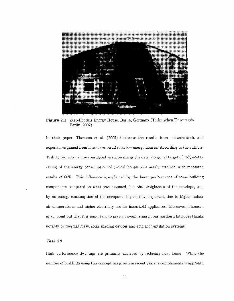
Figure 2.1. Zero-Heating Energy House, Berlin, Germany (Technischen Universitat Berlin, 2007)
In their paper, Thomsen et al. (2005) illustrate the results from measurements and
experiences gained from interviews on 12 solar low energy houses. According to the authors,
Task 13 projects can be considered as successful as the daring original target of 75% energy
saving of the energy consumption of typical houses was nearly attained with measured
results of 60%. This difference is explained by the lower performance of some building
components compared to what was assumed, like the airtightness of the envelope, and
by an energy consumption of the occupants higher than expected, due to higher indoor
air temperatures and higher electricity use for household appliances. Moreover, Thomsen
et al. point out that it is important to prevent overheating in our northern latitudes thanks
notably to thermal mass, solar shading devices and efficient ventilation systems.
Task 28
High performance dwellings are primarily achieved by reducing heat losses. While the
number of buildings using this concept has grown in recent years, a complementary approach
11

like the increase of energy gains in very well insulated housing needed to be studied. So,
starting in 2000, Task 28 was implemented to address cost optimization of the panel of
concepts reducing energy losses, increasing available solar gains and efficiently providing
backup in order to achieve the same high performance (Charron, 2005). As a consequence,
twenty-two projects have been built in 11 different countries with a space-heating target of
15-25 kWh/m 2 . The information can be found on the IEA SHC website.
An interesting project was the 20-terrace house complex in Gothenburg, Sweden. The
goal was to show that it was possible to build passive solar houses with very low energy
use and at reasonable prices in a Scandinavian climate, corresponding to some regions of
Canada Charron (2005). The design strategy was to minimize transmission and ventilation
losses and the building envelope is therefore highly insulated. Also, a special care was taken
to neutralize thermal bridges and to ensure the airtightness of the buildings. A mechanical
ventilation system with an efficiency of 80%, an electric resistance of 900 W for the heating
supply and 5 m2 of solar thermal collectors for the domestic hot water supply were used.
The resulting monitored energy demand was about 68 kWh/m 2 (Wall, 2006).
Some other projects were located in cold climate regions. So, to confirm all the potential
of buildings energy efficiency in such regions, Smeds and Wall (2007) studied six key
design characteristics of high performance houses fulfilling IEA Task 28 targets. These
important features were the area to volume ratio, the thermal insulation, the airtightness
of the building envelope, the ventilation system, the windows areas and the shading
devices. In their paper, the authors asserted that they are absolutely all mandatory to
get environmental friendly dwellings with a comfortable indoor climate and low energy
consumptions. Using the computer software DEROB-LTH for dynamic simulations, they
12

compared conventional buildings using typical construction and system designs with:
(i) high performance buildings like Task 28 houses, and (ii) with constructions and systems
that maximize the utilization of renewable energy. Their results indicated that it was
possible to reduce the heating loads by up to 83% and the total energy demand (space
heating, domestic hot water, electricity) by up to 92% for single-family houses.
Task 40
The objective of Task 40, expected to start by October 2008, will be to investigate current
net-zero, near net-zero and very low energy buildings and to develop a common knowledge,
a methodology, tools, innovative solutions and industry guidelines. The idea is to broaden
the NZEH concept into practical reality in the marketplace. A database of realistic case
studies will be presented, with the aim to lower industry resistance to acceptance of these
concepts.
2.2.3 BedZED & Eco-Village development
The Beddington Zero Energy Development (BedZED) is a development of 100 eco-
homes and workspaces in south London (UK), addressing every area of sustainable living.
Residents have been living there since March 2002. All construction materials used were
carefully selected from sustainable sources. 15% were reclaimed, for instance the timber
used in studwork, or recycled, an example being the crushed concrete used as road sub-
base. Preference was given to materials sourced within a 50 km radius thus reducing
transportation, cutting fossil fuel consumption, reducing the contribution to global warming
and improving air quality. Embodied energy was also reduced in this way and the regional
economy saw benefits too.
13

Key features of BedZED included active and passive solar design strategies, high insulation
levels, high efficiency windows and a combined heat & power plant fuelled by woodchips from
waste timber that provides electricity and hot water. In addition, a green transport plan that
promotes walking, cycling and the use of good local public transport links was established.
During the first year of occupation, a monitoring of building performance and transport
patterns was realized. Table 2.1 shows substantial reduction of energy consumption with the
UK average for space heating and hot water. Such a comprehensive project with coherent
examples of sustainable living should be a source of inspiration for implementing this in
other countries.
Table 2.1. Monitoring results of BedZED & Eco-Village Development (BedZED & Eco-Village Development, 2007)
Monitored reduction Targeted reduction
Space heating 88% (73%)a 90%
Hot water 57% (44%)a 33%
Electricity 25% 33%
Pipes water 50% 33%
Car mileage" 65% 50%
a New homes built after year 2000 UK Building regulations
Fossil fuel consumption
2.3 Canadian initiatives
2.3.1 Advanced House program
In 1992, with the vision to develop sustainable and energy efficient housing, Natural
Resources Canada (NRCan) launched the Advanced Houses program to study innovative
methods that decrease energy consumptions, provide better indoor environments and reduce
14

the environmental impact of houses (Gerbasi, 2000). Ten houses were built across the
country, with technical requirements beyond the R-2000 standard (NRCan, 2005) as they
also considered the total purchased energy. The objective was to use the half of a typical
R-2000 home's energy, or one quarter of the energy and half the water of a typical Canadian
home. There were also individual targets for space heating, cooling, water heating, lighting,
and appliances (including motors for fans and pumps). The Advanced Houses had to meet
minimum requirements for airtightness, ventilation rates, and lighting energy per floor area.
As illustrated in Table 2.2, 75% of the energy reductions were achieved compared to the
average yearly energy use of typical buildings at this time of 39,000 kWh annually. These
impressive numbers were obtained without a major use of renewable energy as only half
the ten Advanced Houses projects included solar thermal technologies and only two used
PV panels. Indeed, considering the local climate, the NOVTEC house in Montreal had
the lowest energy consumption rating without using any active solar systems since it was
equipped with a prototype ground-source heat pump. Hence, such solutions was highly
recommended by Gerbasi.
The differences between the predicted and the actual energy consumptions can be the result
of the precision of simulations programs or by the lower performances than expected of the
original equipments used in the designs. Since the technology has largely evolved since that
time, both active and passive solar technologies should not be an obstacle anymore for the
broad integration of highly efficient buildings in Canada.
15

Tab
le 2
.2.
Ove
rvie
w o
f th
e A
dvan
ced
Hou
ses
prog
ram
(N
RC
an,
2007
)
Pro
ject
BC
Adv
ance
d H
ouse
S
K A
dvan
ced
Hou
se
MB
Adv
ance
d H
ouse
W
ater
loo
Gre
en H
ome
Ham
ilto
n N
eat
Hom
e In
nova
Hou
se
Mai
son
NO
VT
EC
Hou
se
Mai
son
Per
form
ante
P
EI
Adv
ance
d H
ouse
T
he
Env
iroh
ome
Cit
y
Sur
rey
Sas
kato
on
Win
nipe
g W
ater
loo
Ham
ilto
n O
ttaw
a M
ontr
eal
Lav
al
Cha
rlot
teto
wn
Bed
ford
Pre
dict
ed e
nerg
y co
nsum
ptio
n (k
Wh
/yr)
14
,486
20
,514
17
,685
14
,026
13
,911
16
,649
11
,422
11
,067
13
,997
17
,390
Act
ual
ener
gy
cons
umpt
ion
(kW
h/y
r)
12,2
66
31,3
22
20,4
63
14,9
87
19,8
34
18,0
53
13,2
27
12,0
55
N/A
N
/A
Ene
rgy
inte
nsit
y (k
Wh
/(m
2-y
r))
45.4
91
.9
110.
0 65
.0
49.0
N
/A
59.6
63
.8
- -
PV
cap
acit
y
1.92
k
W
Wat
er
pu
mp
2.6
kW
Wat
er
pu
mp
Wat
er
pu
mp
Sol
ar
ther
mal
Yes
Yes
Yes
Y
es
Yes

2.3.2 Net-Zero Energy Coalition
In 2004, a group of home builders and investors started the Net-Zero Energy Home
Coalition (Net-Zero Energy Home Coalition, 2007). This group of forward looking people
considered how residential energy could be supplied in a sustainable way that minimizes
greenhouse gas emission. They proposed a multiphase approach that included pilot
projects in major urban centers across Canada and a national plan that combines R-
2000/Energy Star or higher energy efficiency standards, with a minimum 3 kW photovoltaic
rooftop array or equivalent renewable energy generation source. Their goal was to have all
new residential buildings designed by 2030 to meet a net-zero energy standard.
2.3.3 Solar Building Research Network
The Solar Buildings Research Network (SBRN) was launched in 2006 by the Natural
Sciences and Engineering Research Council (NSERC) through its Research Network Grant
Program (SBRN, 2007). Led by Concordia University, top Canadian researchers in the
solar technology coming from Canadian universities, Natural Resources Canada (NRCan),
the Canada Housing and Mortgage Corporation (CMHC) and Hydro Quebec joined forces
to develop the solar-optimized homes and commercial buildings of the future. Its vision
is the realization of the solar building operating in Canada as an integrated advanced
technological system that approaches the zero-energy target. Consequently, the Network
leads to the development of innovative solar utilization building systems, load management
techniques and software tools that support solar building design.
17

2.3.4 EQuilibrium Housing
Initiated by the CMHC with the collaboration of some major stakeholders, EQuilibrium
Housing is a pilot initiative that demonstrates a new approach to housing in Canada.
It addresses five key principles for sustainable design such as health, energy, resources,
environment and affordability (EQuilibrium Housing, 2007). The goal is to design a highly
energy-efficient house that provides healthy indoor living for its occupants, and produces as
much power as it consumes on a yearly basis with no environmental impact on land, water
and air. Connected to the electricity grid, these homes are expected to draw power only
as needed and to return excess power back into the system. In February 2007, 12 winning
teams of the sustainable housing competition were awarded 50,000 $ each. This money
will help them to build energy-efficient healthy demonstration homes across Canada. Such
development is expected to contribute largely to the advancement of net-zero energy homes.
2.4 Successful strategies
To translate these successful initiatives into winning strategies for future Canadians
homebuilders, a database taking over the useful information on low energy residential
buildings would constitute a major asset. Yet, such analogous task has already been
investigated by Hamada et al. (2003) with the purpose of the collecting information on
passive and active techniques. Indeed, the authors studied 66 homes built from 1988 to 1997
and allocated in 17 different countries. Seven main categories were considered: the design
guidelines, housing data, environmental data, cost data, energy data, system efficiency and
other data. Details like the performance of the building envelope, solar systems and energy
use were included within the categories. Results showed that four key features (passive
18

solar design, super thermal insulation, high performance windows and airtightness of the
building envelope) were the most frequent strategies to achieve low energy homes. Yet, the
spectrum of energy consumptions varied substantially depending on the design strategies
and the climate. Indeed, annual energy fluctuated from a ratio of one to twenty-five.
In order to eliminate the differing environmental conditions making comparisons difficult,
an interesting method was proposed by Charron (2005). The author rated a design as a
comparison to other typical dwellings built in nearby locations. Results are illustrated in
Table 2.3 and present very useful informations about the accurate design strategies for low
energy residential buildings. They show the remarkable value of the thermal insulation and
the airtightness of the building envelope, as the energy consumption can be reduced by
31% compared to a typical home. Yet, the addition of passive solar strategies does not
raise that number drastically. However, it must be considered that a suitable utilization of
thermal mass to decrease temperature swings as well as shading control devices still imply
a rise of thermal comfort feelings (Athienitis and Santamouris, 2002). However, the best
compromise seems to be the Category E when PV panels and solar collectors are added,
as the average energy reduction soars to 75%. Finally, this illustrates very well that it is
certainly conceivable to achieve net-zero energy homes if passive solar elements and heating
system strategies are adequately chosen and assessed.
2.5 Solar water heating systems
Using the sun's energy to heat water is not a new idea. More than one hundred years
ago, in 1891, Clarence Kemp patented and commercialized the world's first solar water
19

Table 2.3. Average energy reduction based on different strategies (Charron, 2005)
Strategies used to reduce Number of Average reduction compared
energy consumptions houses with typical home
Super insulation -f
airtight construction
Category A + passive
solar design
Category A + solar
collectors
Category A + PV
panels
Category A + PV
airtight construction
Category A + other
strategies
heater (DOE, 2008). Since then, the solar water heating technology has greatly improved
and becomes more and more popular every year.
Solar water heating systems (SWHS) are classified as direct or indirect systems (Duffle and
Beckman, 2006). In a direct SWHS system, the thermal collector absorbs solar radiation
energy and transfers this energy to a circulating fluid. The circulating fluid then transfers
the collected energy to a storage device thanks to an internal heat exchanger or, in some
applications like swimming pool heating, to the load directly. In an indirect SWHS system,
there are two separate fluid loops; one collector loop and one tank loop. The energy is
transferred from the collector loop to the tank loop through an external heat exchanger.
2.5.1 Situation of the solar thermal market
Solar thermal applications can be very different in terms of their design (glazed collectors
that include flat-plate and evacuated tube collectors, unglazed collectors for heating
swimming pool water, air collectors, etc.), solar yields and costs. At the end of the year
2006, the solar thermal collector capacity in operation worldwide was equal to 127.8 GW,
31%
33%
59%
45%
75%
61%
20

corresponding to 182.5 million square metres. Of this, 102.1 GW were accounted for by
flat-plate and evacuated tube collectors and 24.5 GW for unglazed plastic collectors. Air
collector capacity was installed to an extent of 1.2 GW (Weiss et al,, 2008). Based on data
collected from detailed country reports, the jobs created by the production, installation and
maintenance of solar thermal plants is estimated to be 150,000 worldwide.
However, it is observed that the market penetration of solar thermal energy varies greatly
depending on the location in the world (Table 2.4)). Indeed, there is a huge gap between the
European countries and Canada. Climatic conditions are obviously different, but a country
like Austria shows that it is quite possible to reach a much higher level of solar thermal
energy contribution, despite being located in the cold environment of central Europe. The
fact is that the adoption of solar thermal applications has been stronger in countries where
there are both national and local long-term policies and support measures. For example, to
counter a slowdown of the solar thermal collector industry in 2002, the German Government
raised the incentives for solar water heating systems from 92 to 125 EUR per m2 of
collector area in February 2003 and thus contributed to improving the market. Locally,
city regulations that require the installation of solar thermal collectors to supply hot water
for buildings have stimulated a rapid growth of such installations, as in the case of the city
of Barcelona in Spain (Aitken, 2003) and (Wiedemann, 2004).
So the question is: Does Canada really have an interest in solar thermal applications?
The answer is not as clear since the huge dependency of the European countries on fossil
fuel makes much more attractive the use of alternative energy sources to decrease the
grade of dependency (Kjarstad and Johnsson, 2007). On the opposite, the hydroelectric
energy is the main source of electricity in Canada, representing nearly two-thirds of all
21

Table 2.4. Market development of flat-plate and evacuated tubular collectors in some countries; installed capacity per year from 1999 until 2006, total capacity in operation in 2006 (absolute and per inhabitant) and the corresponding heat production and CO2 reduction per year (Weiss et al., 2008)
AUT S CH GER DK F CAN USA
Inhabitants [millions] 8.2 9.0 7.3 82.7 5.4 62.3 32.3 298.2
Installed capacity of flat-plate and evacuated tubular collectors
99
107
112
107
117
128
163
207
1,898
231
7
13
15
11
14
14
16
5
165
18
21
18
16
16
15
22
20
27
285
39
294
434
630
378
504
525
665
982
5,638
68
11
9
18
11
6
8
15
32
262
48
17
24
27
49
59
78
92
170
746
12
0
1
1
1
1
1
2
1
58
2
27
26
17
35
36
33
53
80
1,634
5
CO2 emissions avoided by solar plants
Total2oo6 C 0 2 red C 0 2 red
[GW/yr]1
[kt/yr]2
[kg/inhabitant]
1,102
452
54.9
115 178 3,159 132 388
36 70 1,247 51 192
3.9 9.7 15.1 9.4 3.1
179
80
2.5
8,697
4,073
13.7
1 Calculated collector production and corresponding CO2 reduction of all solar thermal systems (hot water,
space heating and swimming pool heating). 2 C02 emissions avoided by solar plants are estimated from the energy savings (oil equivalent). The
emission factor of 2.73 kg C02 per litre of oil is used.
electricity produced (NRCan, 2008). Consequently, thanks to abundant water resources,
electric utilities are able to produce low-cost energy (BC Hydro, 2003), which has a perverse
effect on the general adoption of solar thermal energy in buildings.
Differences between Europe and North American countries are also very well marked in
Table 2.5 as in some countries like Austria (81.9%), Sweden (78.9%) and Germany (91.5%),
solar plants mainly use flat-plate and evacuated tube collectors to prepare hot -water and to
provide space heating, while in the United States (7.9%) and Canada (11.7%), swimming
pool heating is the dominant application with cheaper unglazed plastic collectors.
1999
2000
2001
2002
2003
2004
2005
2006
Totaboo6
Totabocm
[MW th/yr] [MW th/yr]
[MWth/yr]
[MW th/yr]
[MW th/yr]
[MW th/yr]
[MW th/yr] [MW th/yr]
[MWth]
[W*-n /inhabitant]
22

Table 2.5. Distribution of different solar collector by country in operation at the end of 2006 (Weiss et a l , 2008)
18.1
80.7
1.2
21.1
72.1
6.7
34.3
61.7
4.0
8.5
82.4
9.1
5.3
94.0
0.8
8.2
90.4
1.4
88.3
11.3
0.3
92.1
6.0
1.9
AUT S CH GER DK F CAN USA
Unglazed [%]
Flat-plate [%]
Evacuated tube [%]
2.5 .2 E n e r g y s torage
Storage of thermal energy is critically important in many engineering applications. The
problem is particularly true for solar applications since most of the energy is required when
the solar availability is minimum, typically in winter. Therefore, to insure the continuity
of a thermal process, technologies have to able to collect and store the excess heat during
periods of bright sunshine for a later distribution during phases of high energy demand.
Yet, even today, this concept remains technically challenging even after years of research
and development.
For storing the energy, three techniques have been considered over the years for solar thermal
applications. These are (i) the sensible heat storage (where a change of temperature occurs),
(ii) latent heat storage (where a change of phase occurs), and (iii) thermochemical storage
(where a reversible chemical reaction takes place) (Hasnain, 1998).
The most popular and well-developed technology is definitively the sensible heat storage
(SHS) as it is conceptually the simplest form of storing thermal energy. A SHS consists of a
storage medium, a container and input/output devices. The container must retain storage
material for a future use while limiting heat losses to the environment. The amount of energy
stored is proportional to the difference between the storage input and output (Dincer et a l ,
1997).
23

Unfortunately, the sensible heat storage is the least efficient method for energy storage
because of low heat storage capacity per unit volume of the storage medium (Beasley and
Clark, 1984). Latent heat storage (LHS) systems using phase change material (PCM)
as storage medium offer advantages such as high heat storage capacity, small unit sizes
and isothermal behavior during charging and discharging processes (Nallusamy et al.,
2007). However, these types of systems are still in the development process and are not in
commercial use as much as SHS.
2.5.3 Seasonal storage
A storage system collecting from hot summer to use in the winter is called a seasonal
storage. The objective is to increase the solar fraction, defined as the fraction of heating
needs that can be covered by solar, as high as possible (Duffie and Beckman, 2006). In
Europe, for single family home applications, solutions have been found and are available
on the market since the 1990's (Thomsen et al., 2005). Indeed, configurations for seasonal
storage are essentially the same as those considered for short-term storage (overnight). The
main difference between the two types of systems are in the relatives and absolute sizes
of the water tanks and the solar collectors, as the storage capacity for a seasonal system
must be able to store a maximum part of the energy collected during summer months.
Consequently, the ratio of storage to collector area is always much higher for seasonal
storage systems (Braun et al , 1981). For instance, in a low energy building and depending
on the insulation level and the climatic conditions, a water tank with a volume ranging
from 3 to 30 m3 is used to store enough energy to achieve a 100% solar fraction (Hadorn,
2005).
For solar water heating systems with a seasonal storage capacity, some design alternatives
24

are recommended such as: (i) use of an external heat exchanger for domestic hot water
preparation is necessary to avoid legionella problems Krause and Jaehnig; (ii) select the
optimum tilt angle equal to the latitude (Braun et al., 1981).
2.5.4 Stratification in storage tanks
The hotter the water, the lower the density of the water. Hot water thus naturally and
stably finds its way above layers of cold water. This phenomenon makes it possible
to have stratification, with layers of different temperature in one physical store. The
degree of thermal stratification in the storage tank is a measure of its performance.
High tank performance is achieved by eliminating mixing and when the stratification is
maintained (Duffle and Beckman, 2006). Also, due to heat losses from the surface of the
storage tank, the temperature of water near the vertical walls is lower, which leads to natural
convection currents that affect the temperature of layers (Garg et al., 1985). Therefore, a
sufficient thickness of insulation shall be used to maintain the stratification over a long
period.
One way to enhance the stratification is to use external heat exchangers. Indeed, as opposed
to internal heat exchangers, they avoid to disturb the temperature distribution within the
tank (Dayan, 1997). One other way is to use a rigid inlet stratification pipe (stratifier)
with several outlets, as illustrated in Figure 2.2. This arrangement allows water to exit the
unit at the height with approximately the same temperature in the store, thus maximizing
stratification. Such stratifying devices are typically used with both internal and external
heat exchangers in the solar circuit and for the return from the space-heating loop. Though,
this method requires careful attention since the flow in the tube should be within a limited
range, between 5 and 8 kg/min, otherwise the water comes out at an incorrect height (Shah
25

et al., 2005) and (Andersen et al., 2008).
i " j-Vf JJ»
Figure 2.2. Stratifying device for hot water stores (Solvis, 2007)
2.6 Solar combisystems
Since the end of the 1970's, the use of solar collectors for domestic hot water has increased
continuously, showing that solar heating systems are both technically reliable and well
established. Nowadays, in most countries, the market is still focused on such systems,
which are straightforward and have short pay back times, especially due to good subsidies
in some countries (Weiss et al., 2008). But so-called "solar combisystems", which supply
heat for both domestic hot water and space heating, are still only really noticeable in
Austria, Sweden, Switzerland and Germany (Figure 2.6). Reasons for that, beside others,
might be not sufficiently attractive energy savings as well as too much effort and risks
for installers due to the complexity of many system concepts and products (Thiir, 2007).
26

Also, the building integration of such applications becomes increasingly challenging with
the trend towards large contributions like seasonal storage systems. Appropriate surfaces
have to be found by the architect for large collector areas and correspondingly large storage
volumes, considering both aesthetics and building physics (Weiss, 2003).
Table 2.6. Distribution of different applications by country for the total capacity of flat-plate and evacuated tube collectors in operation at the end of 2006 (Weiss et al., 2008)
AUT S CH GER DK F CAN USA " DHW-SFH [%] 63 65 67 80 86 95 95 100 DHW-MFH and district heating [%] 9 10 8 8 13 1 5 0 Combisystems [%] 28 25 25 12 1 4 0 0_
DHW: Domestic hot water systems; SFH: Single family house; MFH: Multi-family house.
These combisystems are typically coupled with a biomass boiler. Common systems for a
single-family house consist of 15 m2 up to 30 m2 of collector area and a 1-3 m3 storage
tank. The share of the heating demand met by solar energy in these systems is between
20-60% (Weiss, 2003). Yet, a variety of systems concept are present on the market. The
difference in the systems is partly due to the conditions prevailing in the individual countries.
For instance, in the Netherlands, "smallest systems" in terms of collector area and storage
volume are more popular and gas or electricity is primarily used as the auxiliary energy
source. So, a typical solar combisystem consists of 4-6 m m2 of solar collector and a 300 1
storage tank, and therefore, solar energy meets a relatively smaller share of the heating and
hot water demand.
2.6.1 Task 26: Solar Combisytems
The most comprehensive research on solar combisystems was certainly performed in
the frame of Task 26 of the IE A Solar Heating and Cooling Programme (IE A SHC,
27

2007). Between 1998 and 2003, 35 solar experts have collaborated to further study solar
combisystems. A system survey and a comparison of 21 different generic combisystem
configurations were carried out to understand and support the growing market of solar
combisystems in Europe. The ultimate objective was to improve the confidence of the end
user in that technology.
The optimization of 9 systems under the same climatic reference conditions was investigated
by using a sensitivity analysis based on simulation results from the TRNSYS program.
Several design improvements were investigated and some key design strategies were
presented (Tepe et al, 2004) such as: (i) select a low temperature space heating system
like a radiant floor; (ii) keep heat losses of the storage tank as low as possible by adding an
appropriate thickness of insulation; (iii) use energy efficient pumps to decrease the electricity
demand; and (iv) use stratifying devices and external heat exchangers to maintain the
stratification in the storage tank.
Low-flow systems are recommended since they ensure a better temperature distribution in
the storage tank when combined with a stratifier (Frei et al , 2000). So, the mass flow
rate of a typical system has to drop from about 50 to 10-15 kg/h per square metre of
collector (Kenjo et al., 2003). Besides of that, low-flow systems are capable of reducing
equipment and installation costs and they allow equipment to be considerably sized down;
piping and pumps are smaller. Cost advantages are in terms of decreased material costs,
less parasitic pumping power required from the utility and reduced costs with installing
lightweight systems (Dayan, 1997).
28

2.6.2 ALTENER
A follow up project of the Task 26 was the European project ALTENER "Solar
Combisystems" that took place between 2001 and 2003 (Ellehauge, 2003). More than
200 solar combisystems in seven European countries were installed, documented and
theoretically evaluated, and 39 of them were also monitored in detail. The goal of this
project was to demonstrate the state of the art of solar combisystems in practice and to
be able to compare the measured results with the annual calculations performed within
Task 26.
2.7 Conclusions
A lot of research has been conducted to develop new technologies for low energy and even
net-zero energy buildings, especially in the residential sector. Constructions combining
higher level of insulation, air tightness, passive solar design and efficient solar combisystems
seem promise to a bright future. In Europe, the increase in the use of solar collectors
in recent years for domestic hot water preparation has shown that solar heating systems
are a mature and reliable technology. Every day, thousands of systems demonstrate the
possibilities of this ecologically harmless energy source. Motivated by the confirmed success
of these systems for hot water production, an increasing number of homebuilders are
considering solar energy for space heating as well.
Yet, designing a seasonal storage combisystems in a cold climate like Canada seems quite
challenging. Indeed, higher standards of thermal insulation are required to allow the heating
loads to be met at reasonable size of solar collector area and storage tank volume. Innovative
concepts and efficient techniques need to be explored. Therefore, since the heat store is
29

the heart of a solar combisystem, a particular attention should be paid to improve the
thermal stratifications by considering low-flow systems, stratifying devices and external
heat exchanger.
30

Chapter 3
Life cycle performance of a base
case house
In this chapter, the integrated building model of a typical single family house in
Montreal (Quebec) is developed using the simulation program TRNSYS 16. The life cycle
performance of the base case house is carried out by estimating the life cycle energy use, life
cycle emissions and life cycle cost. Several design alternatives that upgrade the life cycle
performance are investigated.
3.1 Description of the base case house
An existing one-storey detached house located in Montreal and built in the 1990's is used
as a base case study house. Its total floor area is about 210 m2. The house is made in
wood-frame structure and brick veneer. Figures 3.1 and 3.2 present the drawings of floors
and elevations. Conventional electric baseboard heaters and an electric storage water tank
heater provide the space heating and domestic hot water requirements.
31

s
E
•«-
-> W
to
11.3
m
Stu
dy
Sitt
ing-
room
r\
G
arag
e
11.3
m W
rwx
Hal
l and
Cor
ridor
Mas
ter
Bed
room
Li
ving
-roo
m
(a)
Bas
emen
t fl
oor
(b)
Fir
st f
loor
Fig
ure
3.1
. B
ase
case
hou
se f
loor
s pl
ans

(a)
Nor
ther
n fa
cade
CO
C
O
(b)
Sou
ther
n fa
cade
(c)
Eas
tern
fac
ade
(d)
Wes
tern
fac
ade
Fig
ure
3.2
. B
ase
case
hou
se f
acad
es p
lans

3.2 Description of TRNSYS components used for modelling
The assessment of energy use is implemented using the transient system simulation program
TRNSYS (SEL, 2007). TRNSYS components are referred to as "Types". They are
configured and arranged using the integrated visual interface known as the TRNSYS
Simulation Studio, while building input data is entered through a dedicated visual interface
(TRNBuild). Due to its modular approach, TRNSYS is widely used for solar and nonsolar
modeling applications (DOE, 2008).
Table 3.1 presents TRNSYS standard and TESS libraries (TESS, 2007) components used
in the simulation. It is performed for a complete year, with a one-hour time step.
Table 3.1. List of TRNSYS types
Type
2
4
9
l i b
l l h
16
25
28 33
56b
65
69
89
515
516
518
646
648 701
754
760
Description
Differential Controller
Storage Tank
Data Reader For Generic Data Files
Tempering valve
Tee piece
Solar Radiation Processor
Printer (output file)
Simulation Summary
Psychometrics
Multi-Zone Building
Online graphical plotter
Effective sky temperature
TMY2 Data Reader
Heating and Cooling Season Scheduler
Hourly Forcing Function Scheduler
Monthly Forcing Function Scheduler
Air Diverting Valve
Air Mixing Valve Basement Conduction
Simple Heating and Humidifying System
Sensible Air to Air Heat Recovery
Name used in Simulation Studio
Heaton, Coolon, Lightson, Shadingon, Lig
Tank
Type9e
Diverter
Tee piece
Typel6g
System printer
Q-total-sum, Q-DHW-sum, Q-HVAC-sum
Type33e
Type56b
Type65d, Type65d-2
Type69b
Type89b
Type515
Type516
Type518
Type646
Type648, Type648-2, Type648-3 'IYpe701
Type754f
Type760a
34

3.2.1 Type 56: Building envelope
The building is divided in two distinct zones: one zone comprising the basement without
the garage and a second zone comprising the main living area. The garage and the attic
are unheated and, therefore, temperatures in these spaces are considered as free-floating.
The total heated floor area is 186 m2 , including a basement of 81 m2 . The house has a
gable roof with a slope of 45° and a ceiling with a total area of 105 m2. Joists and rafters
of 38x89 mm (2x4 in), spaced by 600 mm (24 in) represent the frame of the roof and
the ceiling. Exterior cladding of the sloped part is made of asphalt shingles, while bricks
are used for the gable ends. The ceiling includes a total fiberglass insulation of 203 mm
(8 in) and a gypsum board of 12.7 mm constitutes the interior finish. The overall thermal
resistance of the ceiling is equal to 6.08 (rn2-°C)/W.
The above-ground exterior walls are composed of traditional bricks as cladding, 20 mm
of air space, 25.4 mm (1 in) extruded polystyrene (XPS) sheathing boards, wood studs
frame spaced at 400 mm (16 in) with 89 mm (4 in) of fiberglass batt insulation, 6 mm
polyethylene sheet and 12.7 mm gypsum boards. The resulting thermal resistance is equal
to 4.11 (m2 .°C)/W.
Partition walls are composed of wood studs frame spaced at 400 mm (16 in) with two
gypsum boards of 12.7 mm on each side as finish. 89 mm (4 in) of XPS insulation batts are
considered for the interior wall between the garage and the basement.
Foundation walls are 2.60 m high with a i m depth below grade. They are made of 300 mm
of cast-in place concrete, with 25.4 mm (1 in) of expanded polystyrene batt insulation
(EPS), and 12.7 mm gypsum board as interior finish. The thermal resistance of foundation
35

walls is equal to 1.09 (m2-°C)/W.
The first floor is composed of wood I-joists, 25.4 mm (1 in) of EPS batt insulation, 15 mm
plywood subfloor sheathing, 50 mm of light weight concrete and 20 mm of tile. Gypsum
boards of 12.7 mm thick represent the interior finish of the basement ceiling.
The basement floor is made of 100 mm concrete layer, 25.4 mm (1 in) of EPS batt insulation,
50 mm of light weight concrete and 20 mm of tile. The resulting thermal resistance is equal
to 0.99 (m2-°C)/W.
Exterior windows have aluminium frame and double glazing with the cavity filled by
Argon, which corresponds to a U-Value of 1.4 W/(m2-°C). The front and rear doors are
wooden and the garage door is composed by Polystyrol plastic with a thermal resistance
of 1.89 (m2-°C)/W.
Typical thermal properties of building and insulating materials are taken from ASHRAE
(2005). Table 3.2 presents a summary of different dimensions and thermal resistances of
the building envelope.
For the base case house, only the exterior walls and the ceiling/roof comply with the
minimal thermal resistances stipulated in the Quebec regulation for new buildings (Province
of Quebec, 1992), since the values need to be superior to 5.3 (m2-°C)/W for the
ceiling/roof, 3.4 (m2'°C)/W for above-ground walls, 2.2 (m2-°C)/W for foundation walls,
and 1.2 (m2-°C)/W for the basement floor.
36

Table 3.2. Base case house characteristics
Dimensions
Heated floor area
Heated volume Roof area
Attic volume
Exterior doors
Garage door
Windows area
North/East/South/West
[m2]
[m3]
[m2]
[m3]
[m2]
[m2]
[m2]
[m2]
186.0
483.6
148.6
248
4.5
7.8
14.7
9.1/1.5/4.1/0.0
Thermal resistance of the exterior envelope
Ceiling/roof
Above-ground walls
Foundation walls
Basement floor
Exterior doors (wood)
Garage door (Polystyrol)
Windows {/-value
(m2.°C)/W]
(m2-°C)/W]
(m2-°C)/W]
(m2-°C)/W]
(m2.°C)/W]
(m2.°C)/W]
W/(m2.°C)]
6.08
4.11
1.09
0.99
0.47
1.89
1.40
Aluminium frame, double glazing filled by Argon
Overall thermal resistance [(m2.°C)/W] 3.37
3.2.2 Weather input data
The TMY2 (Typical Meteorological Year version 2) weather file for Montreal is selected.
It is connected with Types 33 and 16 that define respectively the moist air properties and
the solar insolation on all surfaces of the building. Type 69 calculates the effective sky
temperature for long-wave radiations. The different components required to assess weather
conditions are connected to Type 56, as shown in Figure 3.3.
37

TMY2
•
TYPE69b
TYPESSb n i TypeJ6b
/A
TYPE33e
"— J B —I
TYPE16g
Figure 3.3. Weather data components
Impact of ground reflectance
Using appropriate values of ground reflectance (albedo) during the winter season in cold
climates is an absolute necessity, since the energy use can be influenced by reflection of
solar radiation off the snow (Thevenard and Haddad, 2006). Yet, Type 16 allows only one
constant value to input as parameter. Therefore, a monthly estimation of ground reflectance
is performed using an Equation-Type (calculator) to assess the following expression:
= Pn 1 -iV*
N + Ps
N„. N
(3.1)
where the snow-free albedo of ground. Pnosnow
is equal to 0.2 (green grass), Nsnaw is the
number of days with snow depth greater than 5 cm (Environment Canada, 2007), N is the
number of days in the month, and psn0w the snow-covered albedo of ground is equal to 0.4
(typical urban site) (Hunn and Calafell, 1977). Table 3.3 presents the results of monthly
ground reflectance computation. These values are set as input data in the monthly scheduler Type 518, which is connected
38

Table 3.3. Monthly ground reflectance values
Month
Jan
Feb
Mar
Apr
May
Jun
Jul
Aug
Sep
Oct
Nov
Dec
Year
N
31
28
31
30
31
30
31
31
30
31
30
31
Nsnow
24.3
22.4
17.2
2.4
0.0
0.0
0.0
0.0
0.0
0.0
3.3 17.2
Pg 0.36
0.36
0.31
0.22
0.20
0.20
0.20
0.20
0.20
0.20
0.22
0.31
0.25
to the solar radiation processor Type 16, as shown in Figure 3.4.
glMtMMiriltTf • aJBr' 'i . r H
TypeMS TYPE16g Type56b
Figure 3.4. Ground reflectance components
39

3.2.3 Type 701: Basement conduction
A particular effort is made to reproduce accurately the heat transfer from the basement
(four walls and the floor) to the soil surrounding the five surfaces of the basement, as
Type 701 from TESS libraries is applied. The heat transfer is assumed to be conductive
only and moisture effects are not accounted for in the model. The model is based on a
3D finite difference model of the soil and solves the resulting inter-dependent differential
equations using an iterative method. The temperature of the zone side surfaces of the floor
and walls as well as the U-values are set as input data. Parameters like the soil properties
and the conditions outside of the basement (near-field) are presented in Table 3.4. The
soil grid geometry is illustrated in Figure 3.5. The initial soil conditions are calculated
from the Kasuda correlation (Kasuda and Archenbach, 1965). The surface conditions for
the near-field and far-field soil are calculated from an energy balance on the surface plane.
The near-field soil temperatures are affected by the heat transfer from the basement. The
far-field soil temperatures are only affected by the surface conditions (time of year) and
depth.
Table 3.4. Parameters for the basement conduction model
Soil properties
Soil properties
Conductivity
Density
Specific heat
Surface emissivity
Surface absorptance
Conditions outside of the basement (near-field) Mean surface temperature
Amplitude of the surface temperature
Day of minimum surface temperature
[°C] [°C]
[day]
6.3
30.3
11
1 The surface absorptance is assumed equal to 1 — pg,year (from Table 3.3). 2 The mean (average) surface temperature of undisturbed soil, assumed equal to the annual
average temperature.
[W/(m-°C)] 2.42
[kg/m3] 3200
[kJ/(kg-°C)] 0.84
0.9
0.75
40

Far field
O.gO
/02O /0.80 /0.20 /T()3 1.03 . 1,03 , 1,03 . 1.03
10.30
0.40
' Near f eld
(a) Soil volumes in the x and z directions
Far field
0.10
/o.ao
0.30
0.40
•mm: " • : .# / •.jmn.iifjjU.Mii; t'-. » I ' I I » * I yum J i n ^jljip^iiji^litJjSrrTiiLjNiiWjiiWiBM
(b) Soil volumes in the y and z directions
Figure 3.5. Representation of basement walls, with near and far-field
41

Figure 3.6 shows that zone inside surface temperatures for the floor and walls, as well as
the U-values are taken from Type 56. Outside surfaces temperatures are then computed by
Type 701 and sended back to Type 56 as input.
Si r r Si JK SO Si
Tjrpe701
Type36b
Figure 3.6. Connections between Types 56 and 701
Instead of considering a fixed value for the convective heat transfer coefficient between the
soil surface and the outdoor air hc, its value is computed as a function of wind velocity v
using Jurges equation (Duffie and Beckman, 2006):
hc= ( 5.8 + 3.9u if v< 5 m/s
(3.2)
7.1v' .0.78 if v> 5 m/s
where:
hc = convective heat transfer coefficient [W/(m2-°C)]; and
v = wind velocity [m/s].
42

3.2.4 Space heating
A system of independent electric baseboard heaters is installed inside the two zones. It
maintains the following temperature profile during the winter period (from October 1 to
May 15).
— On weekdays:
- from 00:00 to
- from 06:00 to
- from 10:00 to
- from 16:00 to
- from 23:00 to
— On weekends:
- from 00:00 to
- from 06:00 to
- from 23:00 to
During the summer period (from May 15 to October 1), the heating system is turned off.
As illustrated in Figure 3.7, these parameters are introduced in Types 515 and 516. The
starting of the heating system is then pondered by a ON/OFF differential controller (Type
2), assuming a dead band value of 1°C.
06:00, Tset = 19°C
10:00, Tset = 21°C
16:00, Tset = 19°C
23:00, Tset = 21°C
00:00, Tset = 19°C
06:00, Tset = 19°C
23:00, Tset = 21°C
00:00, Tset = 19°C
43

TypeSlJ ;J -+—+-
Tsetpoint
Type516
Heaton
f Type36b
+ 1
Figure 3.7. Heating system components
3.2.5 Occupancy
A family of four is assumed to occupy the place intermittently. The occupancy parameter
is directly related to the previous temperature schedule since its value is equal to 1 (100%
of the occupants) when the heating temperature setpoint is 21°C, all year long.
3.2.6 Infiltration
Typically, air infiltration rates for new houses in Quebec range from 3.1 achso to
3.9 ach5o (Zmeureanu et al., 1998b). Therefore, the airtightness of the exterior envelope
is assumed to be in the average for new houses in Quebec and is set to a constant value
3.5 achso in Type 56, for the basement and the first floor.
3.2.7 Space ventilation
A heat-recovery ventilator (HRV) from Venmar (Venmar, 2007) provides the space
ventilation (see technical specifications, Appendix A). The total supply air flow rate is
fixed at the recommended value of 0.35 ach (ASHRAE, 2001), which corresponds for the
house to 169.3 m3/hr. The sensible heat recovery efficiency of the system is a function
44
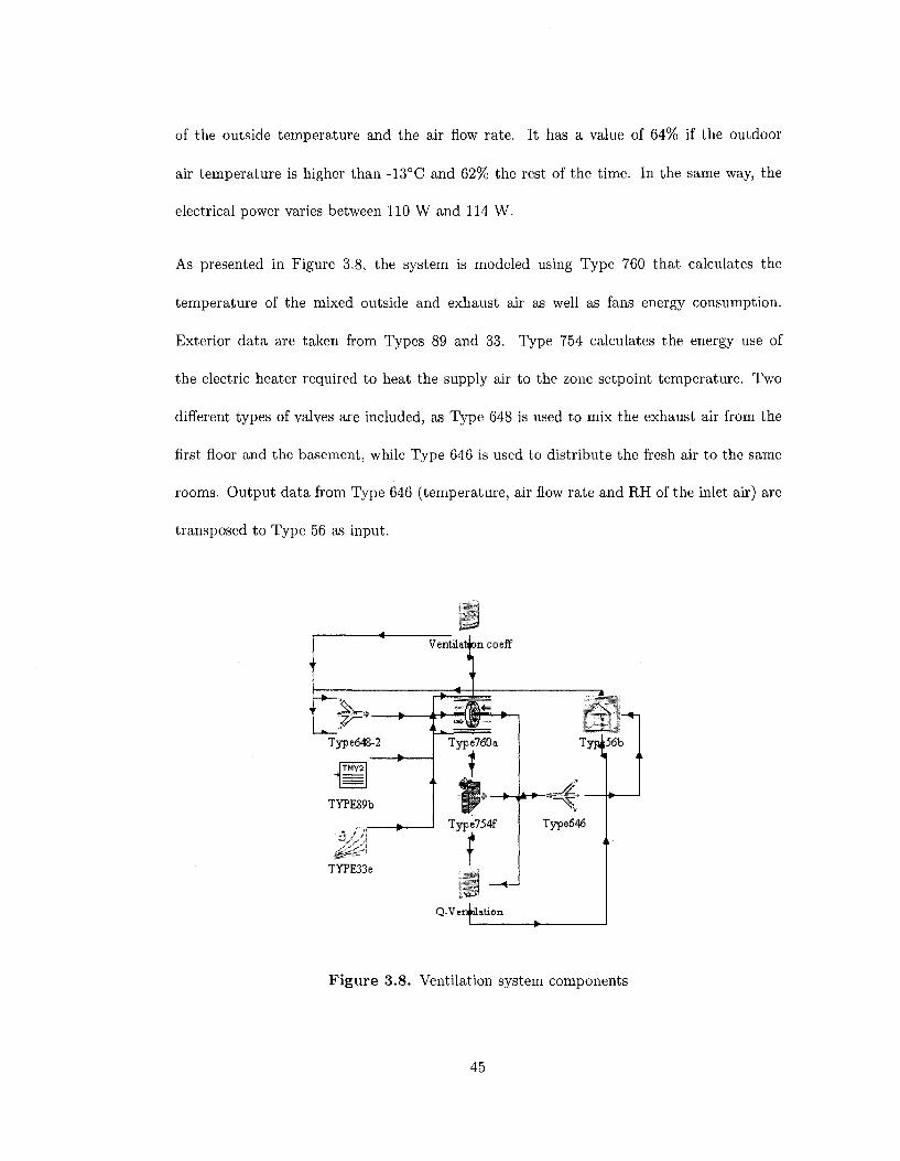
of the outside temperature and the air flow rate. It has a value of 64% if the outdoor
air temperature is higher than -13°C and 62% the rest of the time. In the same way, the
electrical power varies between 110 W and 114 W.
As presented in Figure 3.8, the system is modeled using Type 760 that calculates the
temperature of the mixed outside and exhaust air as well as fans energy consumption.
Exterior data are taken from Types 89 and 33. Type 754 calculates the energy use of
the electric heater required to heat the supply air to the zone setpoint temperature. Two
different types of valves are included, as Type 648 is used to mix the exhaust air from the
first floor and the basement, while Type 646 is used to distribute the fresh air to the same
rooms. Output data from Type 646 (temperature, air flow rate and RH of the inlet air) are
transposed to Type 56 as input.
Ventilation coeff
Type648-2
TMY2
TYPE89b
Jif TYPE33e
• «£=* • ++-J L _
Type760a
I Type754f
"A
xnk
Type646
Q-Venialation
Figure 3.8. Ventilation system components
45

3.2.8 Space cooling
Two split type air conditioners (wall mounted) from Fujitsu (2007) are selected to provide
cooling and dehumidification for the first floor and the basement of the base case house.
Each unit has a nominal cooling power of 3.6 kW and a Coefficient Of Performance (COP)
of 3.5. An average air flow rate of 550 m3/h) per unit, blown at a supply temperature of
14°C and 50% RH, is assumed.
As shown in Figure 3.9, two Types 2 (Coolon-lst, Coolon-base) are used to start the cooling
units if the zone air temperature exceeds typical design values for indoor conditions of
24°C (ASHRAE, 2005). The dead band is fixed at 1°C. The flow rate coming from the
units is then mixed with the air coming from Type 754 (ventilation system) using two
Types 648 in order to consider the first floor and the basement separately. Input data
(temperature, air flow rate and RH of the inlet air) transposed to Type 56 are taken from
Type 648 outputs.
46

i £— " I
Coolon-lst
Type754f
Coolon-base
r*Type64S
Type646 i
^ 6 6 4 8 - 3 "
Q-Cooling
Q-Ventilation
Figure 3.9. Combination of ventilation and cooling system components
3.2.9 Humidification
Using several Types 2 ON/OFF differential controllers (Figure 3.10) and Type 56, an
humidifier is modeled to control the relative humidity of air for the basement and the first
floor. As recommended by Lstiburek (2002), the lower boundary of the relative humidity
in the building has to be limited to 25% in winter. Therefore, when the relative humidity
falls below this limit, the system supplies the minimum value of 25% RH. The dead band
is assumed at 1%.
3.2.10 Shading devices and artificial lighting
In order to assess shading devices and artificial lighting impacts on energy use, different
control strategies as function of exterior solar radiation are assumed.
47

pp. RHset |
4
Humidion-Base
1 Humidon-lst
Type56b
Figure 3.10. Relative humidity control components
Shading devices
In TRNSYS, the modelling of internal devices is detailed including multiple reflection
between the window pane and the shading device (Welfonder et al., 2003). Therefore,
with the perspective to reduce heat loss during winter and to avoid high temperatures
during summer, white opaque curtains are selected. They are located on the inside
surface of all exterior windows. The textile is assumed to have an approximate thermal
resistance of 0.24 (m2 ' °C)/W (Pierce, 2000). Since shades solar-optical properties are taken
from ASHRAE (2005), the transmittance is fixed to zero, the reflectance to 0.65 and the
absorptance to 0.35. These parameters are considered as input data in Type 56.
Type 2 and Type 16 are used to control the opening and closing of the shading devices.
At night, they are considered as always closed. During the day of winter months, they are
assumed to be open when the solar radiation on the south facade is superior to 140 W/m 2 ,
and closed when it is inferior to 120 W/m 2 . During the day of summer months, the opposite
situation occurs since they are closed when the solar radiation on the exterior wall is superior
to 140 W/m 2 , and open when it is inferior to 120 W/m 2 . These boundary values are assumed
48

from default values proposed in Type 56 and from van Moeseke et al. (2007) study.
Artificial lighting
A similar procedure simulates the artificial lighting inside the house. This time, Type 2 and
Type 16 are used to turn the lights on when the total horizontal solar radiation is lower
than 120 W/m2 during daytime, and turn them off when it is higher than 200 W/m2. These
boundary values are assumed from default values proposed in Type 56. Assuming typical
incandescent lights, the total electric input is assumed at 250 W for the first floor, and
125 W for the basement.The combination of shading and lighting components is presented
in Figure 3.11.
Light Thresholds r Ligjit+Shsding
56b
-« 1 s#
Lightson
a t j _ |
ShaimgonS
TYPE16g
Figure 3.11. Shading devices and lighting components
3.2.11 Internal heat gains
Internal heat gains related to the occupancy parameter, lighting and household appliances
are taken into account in the simulation, using Type 56 to specify the different input data.
49

Occupants
Internal heat gains due to occupancy are computed for the first floor and the basement,
using different control strategies. Indeed, three people are assumed to be on the first floor
and one on the basement when the building is occupied. Heat gains per occupants are
specified using the proposed alternatives in Type 56. The option considering people under
the "seated, light work, typing" condition is chosen.
Artificial lighting
The total heat gain due to artificial lighting is computed using Type 56, assuming
that the total electric input of incandescent lamps is converted to 10% of convective
gains (EnergyPlus, 2007).
Household electrical appliances
A 230 W personal computer (with color monitor) the only appliance considered in the
calculation. It is assumed to run on the basement level when the occupancy parameter is
equal to 1.
3 .2 .12 D o m e s t i c ho t w a t e r s u p p l y
The domestic hot water (DHW) is supplied by an electric water heater of 303 1
(80 gallons) located on the basement, with an average tank loss coefficient assumed equal to
0.8 W/(m2-°C). The storage tank, divided in 6 nodes of 10 in (25.4 cm) each, is simulated
in TRNSYS using Type 4.
Two heating elements maintain the water to a setpoint temperature of 55°C. The cold water
inlet is located in the bottom part of the tank and the hot water outlet at the top. The flow
50

rates of water entering and leaving the storage tank are set equal to the consumption profile
values. Two types of valves, a tempering valve and a tee piece, are used to ensure the mix
of cold and hot water. The loss of heat from piping is not considered in the simulation.
DHW consumption profile
The DHW consumption profile is based on a report presented by Jordan and Vajen (2001)
that was initially developed within the scope of the International Energy Agency (IEA,
Task 26: Solar Combisystems). It consists of values of the DHW flow rates, selected by
statistical means, for every hour of the year assuming a mean daily load of 266 1/day (Aguilar
et al., 2005). As an example, flow rates from January 10 to January 13 are presented in
Figure 3.12.
120
100
80
e 3 60 o c X o
40
20
0
Figure 3.12. Sequence of the DHW profile from January 10 to January 13
51
13 25 37
Hours [hi
49 61

City line water temperature
Temperature of cold water from the city line is based on measured data from an aqueduct
located in Montreal (ASHRAE Montreal Chapter, 2007), between years 1994 and 2004.
These data are correlated using the graphing tool FindGraph (UNIPHIZ Lab, 2007) in
order to predict the temperature Tcuy for every hour of the year. The best fit equation
(Equation 3.3) proposed by the program is a Fourier series with 17 harmonics. Coefficients
used in the equation are presented in Appendix B. Figure 3.13 illustrates measured data
and the plot of the best fit equation.
Tcity = a + ci cos(bN) + dx sin(WV) + c2 cos(2bN) + d2 sin{2bN) + ••• (3.3)
25 T _ - n
1 51 101 151 201 251 301 351
Day of the year
Figure 3.13. Temperature of cold water from the city line
52
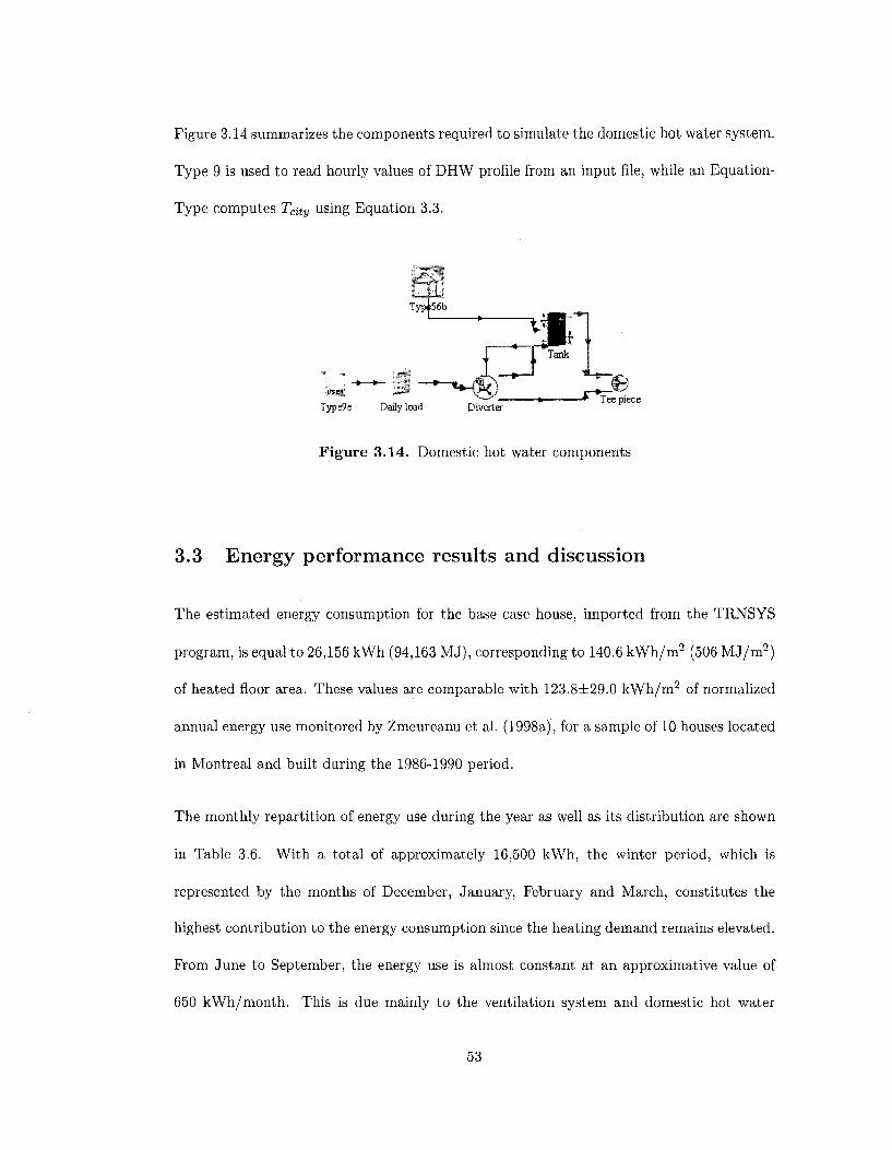
Figure 3.14 summarizes the components required to simulate the domestic hot water system.
Type 9 is used to read hourly values of DHW profile from an input file, while an Equation-
Type computes Tcay using Equation 3.3.
Typi56b
Type9e Daily load ;3 -*-^$£}~*'
Tank
Diverter Tee piece
Figure 3.14. Domestic hot water components
3.3 Energy performance results and discussion
The estimated energy consumption for the base case house, imported from the TRNSYS
program, is equal to 26,156 kWh (94,163 MJ), corresponding to 140.6 kWh/m2 (506 MJ/m2)
of heated floor area. These values are comparable with 123.8±29.0 kWh/m2 of normalized
annual energy use monitored by Zmeureanu et al. (1998a), for a sample of 10 houses located
in Montreal and built during the 1986-1990 period.
The monthly repartition of energy use during the year as well as its distribution are shown
in Table 3.6. With a total of approximately 16,500 kWh, the winter period, which is
represented by the months of December, January, February and March, constitutes the
highest contribution to the energy consumption since the heating demand remains elevated.
From June to September, the energy use is almost constant at an approximative value of
650 kWh/month. This is due mainly to the ventilation system and domestic hot water
53

preparation.
Table 3.6. Monthly repartition and distribution of energy use
Energy use
[kWh]
Heating
Ventilation
DHW
Lighting
Humidification
Cooling
Total
Jan
3,505
717
499
136 211
-
5,068
Feb
2,594
635
443
111
178
-
3,961
Mar
2,044
632
507
102
122
-
3,406
Apr
1,164
495
399
88
31
-
2,178
May
320
360
298
72
-
-
1,050
Month
Jun
-
285
290
65 -
29
668
Jul
-294
194
67
-
100
656
Aug
-294
182
80
-
45
600
Sep
-
285
288
97
-
6
677
Oct
636
466
384
126 1
-
1,613
Nov
1,369
554
352
143
43
-
2,462
Dec
2,276
687
542
143
169
-
3,817
The annual distribution of energy consumption is detailed in Figure 3.15. The heating
system represents the highest contribution to the energy consumption as it counts for 53.2%
of the total value, followed by ventilation with 21.8%, domestic hot water with 16.7%,
lighting with 4.7% and humidification with 2.9%. The contribution of cooling is insignificant
compared to other components.
Humidification 2.9%
Cooling 0.7%
Ventilation 21.8%
Lighting 4.7%
Heating 53.2%
Figure 3.15. Annual distribution of energy use
54

As illustrated in Figure 3.16, the energy signature of the base case house is estimated by
assuming a simple linear regression between the hourly heating energy consumption and
the corresponding hourly outdoor dry-bulb temperature:
Qheating — a + b Tat, (3.4)
where:
Cheating
a
b
Tab
energy use for space heating [kWh];
y-intercept [kWh];
slope [kWh/°C]; and
dry-bulb temperature [°C].
Using data from TRNSYS, the model obtained gives a equal to -0.146 kWh and b equal to
2.467 kWh/°C, with a coefficient of determination R2 of 0.743.
¥ 2, T3
I
Ele
ctri
c de
l
. . ftft—
8.0 H
'• ' •' .,< ; / ; ' ' ' • , ,. 7.0 i
^ :-% / • * ' • • • . • • ' • ' : : * • .
^ ^ 1 « * i t ** ** * **»* • * *
' ' \ i » V ' ***'*'%*>'• ** ** * ,6.0.-
' ••'•'••^SHHL
y = -0.1463X + 2.4676 Rz = 0.7437
- *- ?«5MKf«SBBBgBSft. r -.. •' '^W&eBNBtix&t>*. • "T&^Q9HEB£§HHfri'i '.'•
'') V'.TJ"! BBHSWffiBU*:*?:';.. .•' * # %^S 7
1.0*''-
, 1 0.0
^^^^^mmV^mHpfr^i^t'"
^HPffifeV*'*-' "' * *r*q|fiB^8p&.<as..
-35.0 -25.0 -15.0 -5.0 5.0 15.0
Outdoor dry-bulb temperature [°C]
25.0 35.0
Figure 3.16. Energy signature of the base case house
55
In order to illustrate interior conditions in the base case house, Figures 3.17 and 3.18 show
air temperature and relative humidity profiles coming from TRNSYS, for a period of three
days in the beginning of February and July, respectively. In February, temperatures vary
as expected between the two setpoint values of 19 and 21°C and the humidification system
appears to operate a majority of time, fixing the relative humidity to the design value of 25%.
On some occasions during the month of July, the temperature and the relative humidity on
the basement are superior to values on the first floor. In a general way, temperatures range
between 21 and 24°C, and the relative humidity between 40 to 60%.
56
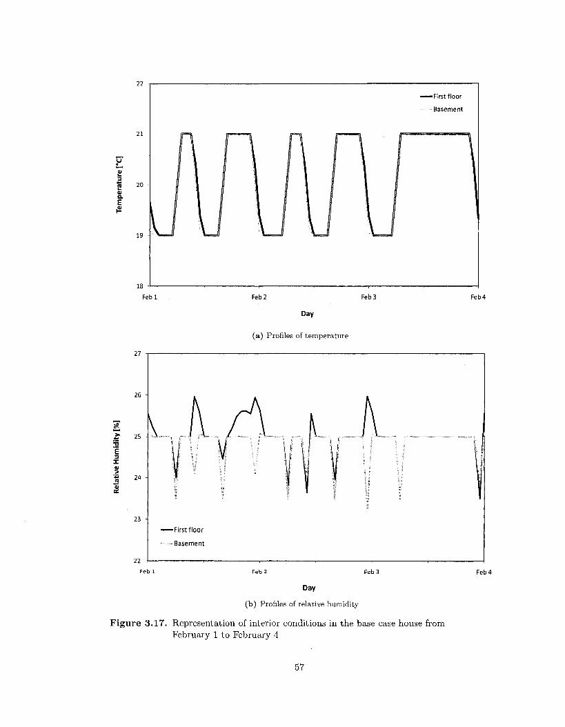
22
IS
Febl
27 7
26 H
I" 0£
V
23 i
22 4
-First floor
Basement
Feb 2
Day
(a) Profiles of temperature
Feb 3 Feb 4
-First floor
Basement
Feb 2 Feb 3 Feb 4
Day
(b) Profiles of relative humidity
Figure 3.17. Representation of interior conditions in the base case house from February 1 to February 4
57

26
25 i
22 A
21 Jul 1
60
55 H
35
Jul 1
Jul 2
Day
(a) Profiles of temperature
Jul 3
Jul 3
-First floor
Basement
Jul 4
-First floor
Basement
Jul 4
Day
(b) Profiles of relative humidity
Figure 3.18. Representation of interior conditions in the base case house from July 1 to July 4
58

3.4 Life cycle analysis of the base case house
This section presents the life cycle analysis of the base case house in terms of the following
indicators: life cycle energy use, life cycle emissions and life cycle cost.
3.4 .1 Life cyc le e n e r g y use
The life cycle energy use includes the total energy input over the entire life cycle of a
building or its subsystems. Within the scope of this study, the embodied energy due to the
manufacturing of the building materials in the pre-operating phase, and the total energy
use in the operating phase are evaluated.
It is important to notice that: (i) the embodied energy of plumbing, heating, cooling and
ventilation systems are not taken into account, and (ii) the estimation does not consider
energy used for maintenance and demolition.
Embodied energy
The embodied primary energy, that represents direct and indirect energy use to extract raw
materials, transport and fabrication of the final product, is estimated using the ATHENA's
Environmental Impact Estimator software (ATHENA, 2003). This tool also operates the
assessment of the building's GHG emissions, starting at its conception over its expected
lifetime. Therefore, global warming potentials (GWPs), that constitutes a reference measure
to compare the global warming effect of 1 kg of a given gas to the effect of 1 kg of CO2 over
a 100-year life span (IPCC, 2007), are computed.
The information from drawings and specifications is used to define the constituting
assemblies and materials. These input data are then linked by ATHENA to the life cycle
59
inventory database for calculation. The building is located at Montreal (Quebec) and its
life expectancy is assumed at 30 years.
The total embodied energy of the base case house is assessed at 566,907 MJ, corresponding
to 2,697 MJ /m 2 of total floor area, and is equivalent to approximately five years of
annual operating energy consumption. For comparison purpose, the results of previous
studies are cited: Haines et al. (2007) estimated the embodied energy of a single-family
dwelling, complying with the Ontario Provincial Building Code, to a value of 520,000 MJ or
2,600 MJ /m 2 of floor area, while Kassab (2002) found a value of 707,883 MJ or 2,286 MJ /m 2
of floor area for duplex-apartment house built in 2000 at Montreal, and finally, Baouendi
(2003) estimated the embodied energy of a one-story detached house at 330,316 MJ or
1,278 M J / m 2 of heated floor area. Major differences are observed with the last study
but, generally speaking, a comparison is not easy since the buildings may have different
dimensions, structural configuration of the exterior envelope constructions and locations.
The embodied energy per envelope component is shown in Table 3.8. The exterior and
foundation walls presents the highest embodied energy (1574 MJ /m 2 of wall area), followed
by floors and roofs (637 MJ/m 2 ) , foundations (355 MJ /m 2 ) , and doors and windows
(239 MJ /m 2 ) . The average weighted embodied energy is assessed at 836 MJ/m 2 .
60
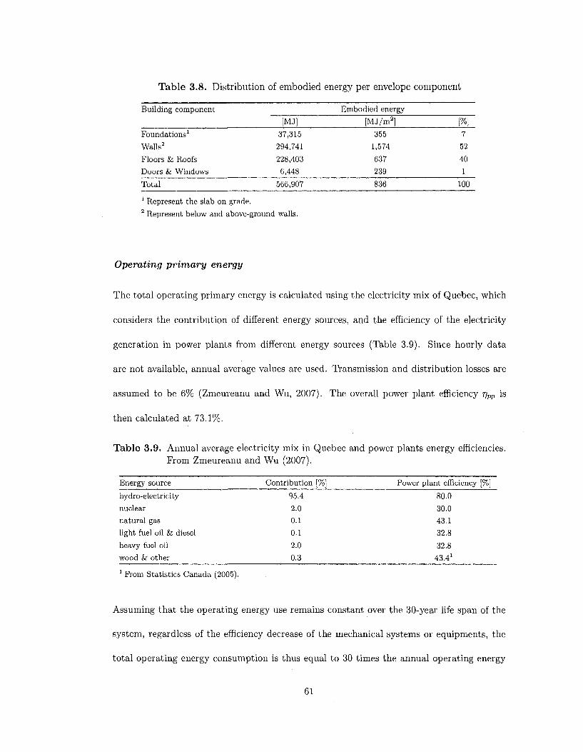
Table 3.8. Distribution of embodied energy per envelope component
Building component
Foundations1
Walls2
Floors & Roofs
Doors & Windows
Total
[MJ] 37,315
294,741
228,403
6,448
566,907
Embodied energy
[MJ/m2]
355
1,574
637
239
836
{%} 7
52
40
1
100
1 Represent the slab on grade. 2 Represent below and above-ground walls.
Operating primary energy
The total operating primary energy is calculated using the electricity mix of Quebec, which
considers the contribution of different energy sources, and the efficiency of the electricity
generation in power plants from different energy sources (Table 3.9). Since hourly data
are not available, annual average values are used. Transmission and distribution losses are
assumed to be 6% (Zmeureanu and Wu, 2007). The overall power plant efficiency r\PV is
then calculated at 73.1%.
Table 3.9. Annual average electricity mix in Quebec and power plants energy efficiencies. From Zmeureanu and Wu (2007).
Energy source Contribution [%] Power plant efficiency [%]
hydro-electricity 95.4 80.0
nuclear 2.0 30.0
natural gas 0.1 43.1
light fuel oil & diesel 0.1 32.8
heavy fuel oil 2.0 32.8
wood & other 0.3 43.41
1 From Statistics Canada (2005).
Assuming that the operating energy use remains constant over the 30-year life span of the
system, regardless of the efficiency decrease of the mechanical systems or equipments, the
total operating energy consumption is thus equal to 30 times the annual operating energy
61

use. Its value is estimated at 3,864 GJ, corresponding to 18,382 MJ/m2 of floor area. The
total life cycle energy use of the base case house, calculated as the sum of its embodied
energy and the operating energy use over 30 years, is equal to 4,431 GJ.
3.4.2 Life cycle emissions
Embodied emissions
The embodied emissions of the base case house are evaluated at 29.75 tons CO2 eq.
by the software ATHENA. The distribution per envelope component is shown in Ta
ble 3.10. The exterior and foundation walls presents the highest embodied energy
(73 kg CO2 eq./m2 of wall area), followed by doors and windows (38 kg CO2 eq./m2),
foundations (35 kg CO2 eq./m2), and floors and roofs (32 kg CO2 eq./m2). The average
weighted embodied energy is assessed at 44 kg CO2 eq./m2.
Table 3.10. Distribution of embodied emissions per envelope component
Building component
Foundations1
Walls2
Floors & Roofs
Doors & Windows
Total
[kg CO2 eq.]
3,674
13,600
11,442
1,031
29,747
Embodied emissions
[kg C 0 2 eq./m2]
35
73
32
38
44
[%] 12
46
38
3
100
1 Represent the slab on grade. 2 Represent below and above-ground walls.
Operating emissions
The emissions of pollutants due to the house operation are investigated by considering the
contribution of each energy source to the off-site production of electricity (Table 3.9) as well
as the transmission and distribution losses. Therefore, the greenhouse gases emissions due
62

to electricity generation in power plant are estimated using the equivalent CO2 emissions
data presented by Gagnon et al. (2002). The following expression is calculated:
Oi\Ehydro + Oi2Egas + a^Eoil + (X/iEcoal + ®5Enuclear /„ Rx
C02,pp - — (3.5)
where:
— C02,pp is the equivalent CO2 emissions at the generating power plant level [kg CO2 eq.];
- Ehydro, Egas, E0u, Ecoal, Enuciear, correspond to the annual primary energy generated
by hydro, natural gas, heavy oil, coal, and nuclear power plant respectively [kWh/yr];
— ai_5 are the equivalent CO2 emissions due to the generation of electricity in power
plants [kt C02/TWh];
— ot\ = lb kt CO2/TWI1, for hydro power plant with reservoir;
- a2 — 443 kt CO2/TWI1, for natural gas (+ 2000 km delivery) power plant;
— Q!3 = 778 kt CO2/TWI1, for heavy oil power plant;
- Oj = 1050 kt CO2/TWI1, for modern coal (2% S) power plant with SO2 scrubbing;
- a$ = 15 kt CO2/TWI1, for nuclear power plant.
Consequently, for the base case house, the annual operating emissions are estimated at
1,875 kg CO2 eq. annually and at 56.24 tons CO2 eq. over the 30-years building's lifetime.
The life cycle emissions are equal to 85.98 tons CO2 eq. The embodied emissions represent
35% of the life cycle emissions while the embodied energy represents only 13% of the total
life cycle energy use. This can be explained by the fact that the energy used to manufacture
63

materials and transport produce more emissions per unit of energy than the energy used
for the house operation, due to the low impact on the environment of hydro power plants
in Quebec.
3.4.3 Life cycle cost
Construction phase
The initial cost of the base house is estimated using Residential Cost Data from RSMeans
(2007), including the total cost of building materials, labor, contractor profit and overhead
cost. Seven categories are identified including: site work, foundation, framing, exterior walls,
windows and doors, roofing and interior partitions. Costs are taken from the assemblies
and materials tables listed in the database. Then, total costs are multiplied by a city factor
to account for the impact of the local market (1.21 for Montreal) and divided by a factor
of 1.01 to assume the present exchange rate from US dollars to Canadian dollars. The
construction cost of the base case house is finally evaluated at 204,576 $ or 973 $/m2 of
floor area.
Operating phase
Typically, operating costs include energy and maintenance costs during the life span of the
building, along with demolishing costs at the end of the building life. However, for this
study, only the cost of the energy use is considered. The annual energy use is supposed to
remain constant during the lifetime of the building.
The heating cost is calculated with respect to the electricity rates of Hydro-Quebec (2008)
as follows:
— 0.4064 $ as a fixed charge per day; plus
64

- 0.0540 $ per kWh for first 30 kWh per day; plus
— 0.0733 S per kWh for the remaining consumption.
The Present Worth method (PW), which converts any present and future expenses to the
same basis on today's dollars, is applied to evaluate the present value of money for the total
operating energy cost over the life cycle of the building. The following equation (ASHRAE,
2007) is used:
Cjl+JE)"-1
PWN = \JJ*> (3.6)
where:
PWN = present worth of operating energy cost at the end of the year N [$];
C = operating energy cost during the first year [$];
JE = inflation rate of electricity [-];
i' — effective interest rate [-]; and
N = number of years [-].
The effective interest rate i' is calculated as:
'-TTi M
where:
i = discount rate (including inflation) [-]; and
j = inflation rate [-].
65

Finally, the Present Worth over JV years is:
N
pw = j2 PWN (3-8)
The price of electricity is assumed to increase by 2% each year. Average values of the
discount rate and the interest rate from 1998 to 2008 are used (Statistics Canada, 2008).
So, i = 5.54%, j = 2.24% and the resulting value of i' is 3.22%. Based on TRNSYS
simulation results, the annual operating cost is equal to 1,878 $ (9 $/m2) and the PW over
the life cycle period of 30 years is calculated at 46,193 $ (220 $/m2).
3.4.4 Summary of the results
The results obtained from previous sections are summarized in Table 3.13.
Table 3.13. Life cycle profile of the base case house
Life cycle energy use
Life cycle emissions
Life cycle cost
[GJ]
[%] [tons CO2 eq.]
[%] [$]
[%]
Construction phase
567
13
29.75
35
204,576
82
Operating phase
3,864
87
56.24
65
46,193
18
Life cycle
4,431
100
85.98
100
250,769
100
3.5 Life cycle analysis of design alternatives
In this section, several design alternatives are proposed in order to quantify their potential
effect on a life cycle perspective. The thermal resistance of the exterior envelope of the
base case house is improved to different levels of insulation. In addition, modifications on
window-to-wall ratios (WWR) and infiltration rates are investigated.
66

3.5.1 Improvement of the thermal resistance of the building envelope
Choice of insulation materials
In order to facilitate the selection of design alternatives, a comparison between common
insulation materials presenting the same thermal resistance of 3 (m2-°C)/W in terms of
embodied energy, embodied emissions and costs, is illustrated in Table 3.14. Results are
taken from ATHENA (2003) and RSMeans (2007).
Table 3.14. Comparison between typical insulation materials
Insulation
material
Fiberglass batt (108 mm)
EPS (105 mm)
XPS (87 mm)
Blown cellulose (128 mm)
PIR (78 mm)
Embodied energy
[MJ/m2]
83.25
180.33
297.52
9.79
1.56
Embodied emissions
[kg C 0 2 eq./m2]
3.93
7.88
13.05
0.40
2.81
Cost
[$/m2] 6.07
23.36
30.77
8.70
29.10
The PIR (polyisocyanurate) has the lowest embodied energy with 1.56 MJ/m2, in opposition
with the XPS (extruded polystyrene) with 297.52 MJ/m2, while the blown cellulose has
almost zero embodied emissions, compared with 3.93 kg CO2 eq./m2 for the fiberglass batt.
Table 3.14 emphasizes very well the fact that building designers need to be cautious with
their choice of insulation materials since the overall performance, and not only the thermal
resistance or cost, has to be considered in a sustainable approach.
Presentation of selected design alternatives
The first two design alternatives are elaborated to comply with the minimum insulation
levels according to the Quebec Energy Code (Province of Quebec, 1992) and the Model
National Energy Code of Canada for Houses (MNECCH, 1997).
67

Since the windows area of the base case house is quite low, a third alternative presenting
similar insulation materials than the second one, but that with larger windows on the
south facade, is suggested. Therefore, the window-to-wall ratio, which is the proportion of
window area compared to the total wall area where the window is located (DOE, 2008), is
increased from a value of 0.09 to 0.20 on the south facade to maximize solar heat gains.
This alternative is named MNECCH+.
One last alternative, called "best case", is proposed in order to meet higher insulation
levels with an particular emphasis aimed at "sustainable" insulation materials. Therefore,
based on the analysis of Table 3.14, blown cellulose and polyisiocyanurate are preferred. All
windows are upgraded using the best double-glazed window available in TRNSYS library,
corresponding to a U-value of 1.26 W/(m2-°C). The WWR is kept at a value of 0.20 for the
south facade, similarly to the MNECCH+ alternative. The air infiltration rate is reduced
at 1.5 acli5o, as recommended by the R-2000 program (NRCan, 2005). To achieve this
objective, sprayed applied PIR is assumed to fill the gaps around windows and doors, at
the junction of the main floor framing and the foundation, at tops of exterior and partition
walls.
Table 3.15 reviews the thermal resistance and U-value of each component of the building
envelope for all the studied design alternatives. The resulting overall thermal resistance
(weighted average) is presented.
The thermal resistance of each component of the envelope is calculated using different
insulation materials. Table 3.16 summarizes insulation materials and related thickness used
for each component and design alternative. Proposed design alternatives are established
with the perspective to comply with the minimum resistance required by the code. It
68
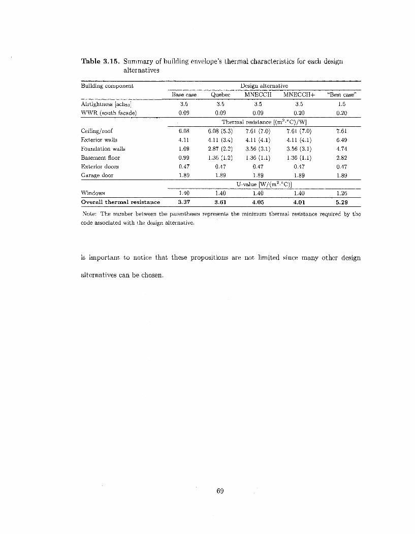
Table 3.15. Summary of building envelope's thermal characteristics for each design alternatives
Building component
Airtightness [achso]
WWR (south facade)
Base case
3.5
0.09
Quebec
3.5
0.09
Design alternative
MNECCH MNECCH+
3.5 3.5
0.09 0.20
"Best case"
1.5
0.20
Thermal resistance [(m2-°C)/W]
6.08 (5.3)
4.11 (3.4)
2.87 (2.2)
1.36 (1.2)
0.47
1.89
7.61 (7.0)
4.11 (4.1)
3.56 (3.1)
1.36 (1.1)
0.47
1.89
7.61 (7.0)
4.11 (4.1)
3.56 (3.1)
1.36 (1.1)
0.47
1.89
7.61
6.49
4.74
2.82
0.47
1.89
U-value [W/(m2-°C)]
Windows
Overall thermal resistance
1.40
3.37 1.40
3.61 1.40 1.40
4.05 4.01
1.26
5.29
Note: The number between the parentheses represents the minimum thermal resistance required by the
code associated with the design alternative.
is important to notice that these propositions are not limited since many other design
alternatives can be chosen.
Ceiling/roof 6.08
Exterior walls 4.11
Foundation walls 1.09
Basement floor 0.99
Exterior doors 0.47
Garage door 1.89
69

Table 3.16. Insulation materials used in design alternatives
Alternative
Base case
Quebec
MNECCH
MNECCH (WWR+)
"Best case"
Ceiling/roof
203 mm batt
203 mm batt
305 mm CEL
305 mm CEL
305 mm CEL
Exterior wall
89 mm batt
+25.4 mm XPS
89 mm batt
+25.4 mm XPS
89 mm batt
+25.4 mm XPS
89 mm batt
+25.4 mm XPS
89 mm SPIR
+50.8 mm PIR
Foundation wall
25.4 mm EPS
25.4 mm EPS
+63.5 mm batt
25.4 mm EPS
+89 mm batt
25.4 mm EPS
+89 mm batt
25.4 mm EPS
+89 mm SPIR
Slab on grade
25 mm EPS
38 mm EPS
38 mm EPS
38 mm EPS
89 mm EPS
Notes: CEL represents the blown cellulose and SPIR the spray applied polyisiocyanurate (PIR).
Using the computer programs TRNSYS, ATHENA and the RSMeans database, the life
cycle energy use, emissions and cost are estimated for each design alternative. A summary
of results is shown in Table 3.17 as well as savings compared with the base case house.
70

Tab
le 3
.17.
Su
mm
ary
of p
erfo
rman
ce o
f pr
opos
ed d
esig
n al
tern
ativ
es
Des
ign
alte
rnat
ive
Bas
e ca
se
Que
bec
MN
EC
CH
MN
EC
CH
+
"Bes
t ca
se"
Life
Em
bodi
ed
567
571
+0.
7%
558
-1.6
%
569
+0.
3%
546
-3.9
%
cycl
e en
ergy
use
Ope
rati
ng
129
119
-8.5
%
117
-10.
5%
115
-11.
5%
93
-38.
9%
[GJ]
Life
cyc
le
4,43
1
4,13
2
-7.2
%
4,05
6
-9.2
%
4,03
3
-9.9
%
3,32
7
-33.
2%
Life
cyc
le
Em
bodi
ed
29.7
5
29.9
2
+0.
6%
29.3
0
-1.5
%
29.9
2
+0.
6%
28.8
4
-3.1
%
emis
sion
s [t
ons
Ope
rati
ng
1.87
1.73
-8.5
%
1.70
-10.
5%
1.68
-11.
5%
1.35
-38.
9%
C0
2 eq
.]
Life
cyc
le
85.9
8
81.7
5
-5.2
%
80.2
1
-7.2
%
80.3
5
-7.0
%
69.3
3
-24.
0%
Init
ial
204,
576
208,
173
+1.
7%
209,
247
+2.
2%
211,
001
+3.
0%
212,
569
+3.
8%
Life
cyc
le c
ost
[$]
Ope
rati
ng
1,87
8
1,72
7
-8.8
%
1,69
6
-10.
8%
1,67
7
-12.
0%
1,33
4
-40.
7%
Life
cyc
le
250,
769
250,
644
+0.
0%
250,
951
+0.
1%
252,
239
+0.
6%
245,
390
-2.2
%
Not
e: P
erce
ntag
es r
epre
sent
the
inc
reas
e co
mpa
red
wit
h th
e ba
se c
ase
hous
e.
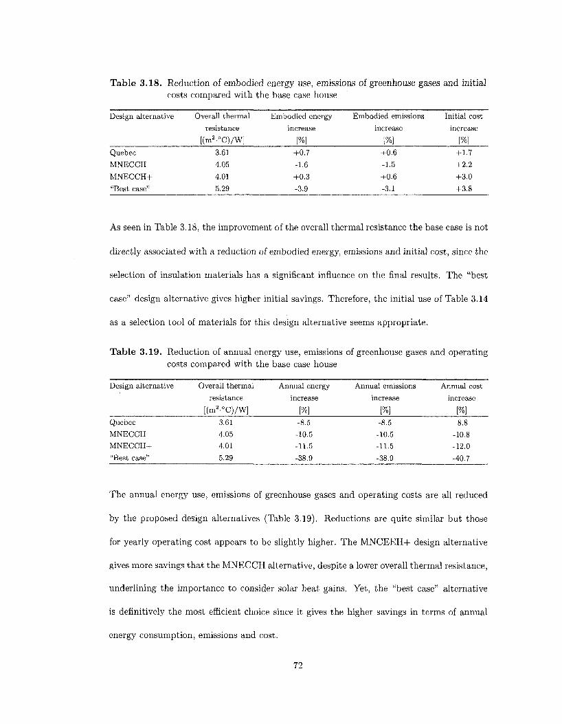
Table 3.18. Reduction of embodied energy use, emissions of greenhouse gases and initial costs compared with the base case house
Design alternative
Quebec
MNECCH
MNECCH+
"Best case"
Overall thermal
resistance
[(m2.°C)/W]
3.61
4.05
4.01
5.29
Embodied energy
increase
[%]
+0.7
-1.6
+0.3
-3.9
Embodied emissions
increase
[%] +0.6
-1.5
+0.6
-3.1
Initial cost
increase
[%} +1.7
+2.2
+3.0
+3.8
As seen in Table 3.18, the improvement of the overall thermal resistance the base case is not
directly associated with a reduction of embodied energy, emissions and initial cost, since the
selection of insulation materials has a significant influence on the final results. The "best
case" design alternative gives higher initial savings. Therefore, the initial use of Table 3.14
as a selection tool of materials for this design alternative seems appropriate.
Table 3.19. Reduction of annual energy use, emissions of greenhouse gases and operating costs compared with the base case house
Design alternative
Quebec
MNECCH
MNECCH+
"Best case"
Overall thermal
resistance
[(m2-°C)/W]
3.61
4.05
4.01
5.29
Annual energy
increase
[%] -8.5
-10.5
-11.5
-38.9
Annual emissions
increase
[%] -8.5
-10.5
-11.5
-38.9
Annual cost
increase
[%] -8.8
-10.8
-12.0
-40.7
The annual energy use, emissions of greenhouse gases and operating costs are all reduced
by the proposed design alternatives (Table 3.19). Reductions are quite similar but those
for yearly operating cost appears to be slightly higher. The MNCEEH+ design alternative
gives more savings that the MNECCH alternative, despite a lower overall thermal resistance,
underlining the importance to consider solar heat gains. Yet, the "best case" alternative
is definitively the most efficient choice since it gives the higher savings in terms of annual
energy consumption, emissions and cost.
72

Table 3.20. Reduction of life cycle energy use, emissions, and cost for the different design alternatives compared with the base case house
Design alternative
Quebec
MNECCH
MNECCH+
"Best case"
Overall thermal
resistance
[(m2.°C)/W]
3.61
4.05
4.01
5.29
Life cycle
energy
[GJ]
-7.2
-9.2
-9.9
-33.2
Life cycle
emissions
[tons CO2 eq.]
-5.2
-7.2
-7.0
-24.0
Life cycle
cost
[$] +0.0
+0.1
+0.6
-2.2
The life cycle energy use and life cycle emissions are reduced for all the proposed design
alternatives (Table 3.20). Life cycle costs for the "Best case" alternative are reduced by
2.2% while costs are similar in other cases. This can be seen as a direct consequence of
the low rates of electricity in Quebec, compared to other Canadian provinces (BC Hydro,
2003). The most significant reductions are those for energy use, ranging from 7.2% to 33.2%.
Higher insulation levels also gives emissions savings but the resulting effect is limited due to
the influence of life cycle performance of some insulation materials. It is interesting to see
that the MNECCH+- alternative offers roughly the same energy savings and emissions as
the MNECCH alternative, despite a higher cost. The "best case" alternative is definitively
the most efficient solution as it gives the higher savings in terms of energy, emissions and
cost on a life cycle perspective.
73

Chapter 4
Modelling of a seasonal thermal
storage
In this chapter, the modelling of a solar combisystem with a long-term thermal storage
capacity, associated with a hydronic radiant heating floor, is presented. The TRNSYS
environment is used for this purpose. The "best case" alternative (see Chapter 3) is
chosen as the starting point in the development of the model. A sensitivity analysis, based
on a certain set of design parameters, is achieved to evaluate the repercussions of those
parameters on the overall performance of the system.
4.1 General description of the system
The long term thermal storage system is designed to supply hot water for space heating
and domestic hot water for one year using only the solar energy, that is without the need
of an auxiliary heating element (Figure 4.1).
74
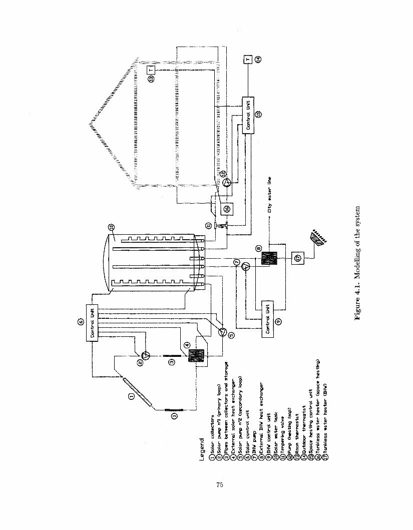
-a
Or
©
Co
ntr
ol
Un
it
©
<D /
T
Le
ge
nd
•—
(l
)So
lar
coll
ecto
rs
(?) S
ola
r pu
mp
n*l
(p
rln
ary
loo
p)
(^P
lpe
s b
etw
een
co
llec
tors
an
d
sto
rag
e
^)E
xte
rna
l so
lar
he
at
exch
ang
er
(^S
ola
r pu
np n
*2 (
seco
nd
ary
loo
p)
@
So
lar
co
ntr
ol
un
it
punp
©E
xte
rna
l DH
W h
eat
exch
ang
er
©D
HW
c
on
tro
l u
nit
(j3)
So
lar
wa
ter
tan
k
(ll)
Tem
peri
ng
valv
e
(@)P
ump
<h
eatl
ng
loo
p)
(l3)R
oon
th
erm
os
tat
(J4)
Ou
tdo
or
ther
mo
stat
(13)
Spa
ce h
eati
ng
co
ntr
ol
un
it
fli)
Tan
kles
s w
ater
he
ate
r (s
pac
e h
eati
ng
)
@T
an
kle
ss
wat
er h
ea
ter
<DHW
)
© A ®
_L _
i_
m
-^®
Co
ntr
ol
Uni
t
©H
i
® ^z
@J~
4-©^
_®
_i_
Co
ntr
ol
Un
it
®
©
Cit
y w
ate
r lin
e
Fig
ure
4.1
. M
odel
ling
of t
he s
yste
m

The combisystem consists of evacuated tube solar collectors (point 1 in Figure 4.1) placed
on the roof of the house, the heat transfer loop and a pump (point 2) that includes the
antifreeze fluid, and the external heat exchanger (point 4) that transfers the heat collected
from the primary loop into a secondary loop where circulates the water. Hot water from
the secondary loop, circulated by a pump (point 5), enters a large cylindrical water storage
tank (point 10). A stratifier device improves the stratification by avoiding the mixing of
layers of different temperature inside the tank. Hot water is supplied to radiant heating
floors of the house by a variable speed pump (point 12) controlled by a thermostat located
on the first floor (point 13). An external heat exchanger (point 8) and a variable speed
pump (point 7) enable the control of domestic hot water at around 45°C at the user-end.
4.2 Heat management approach
4.2.1 Solar loop
Solar energy is captured by evacuated tube collectors since their use is recommended in
cold climates (RETScreen, 2007). The variable flow rate pump (point 5) circulates the
hot water on the secondary loop from the external solar heat exchanger (point 4) to the
tank, at a maximum temperature of 95°C. Both pumps (points 2 and 5) start only when
the inlet temperature of the heat exchanger, on the primary loop, is higher than the water
temperature at the bottom of the tank.
4.2.2 Space heating
The space heating is provided by a hydronic radiant floor heating system as it represents
typically a better choice for low energy buildings (Keller, 1998), it brings higher exergy
76

efficiency (Zmeureanu and Wu, 2007) and increases thermal comfort (ASHRAE, 2004).
Cross-linked polyethylene (PEX) (Liu et al., 2000) flexible piping is integrated in the radiant
floor to circulate the hot water. The garage floor is not heated.
A constant setpoint temperature control is applied on the operative temperature which is a
better indicator of the thermal comfort for radiant systems than the air temperature, while
improving the energy performance (Van der Veken et al., 2005). Therefore, a proportional-
integral-derivative (PID) controller modifies the flow rate of the hot water circulating pump
(point 12) to maintain the operative temperature on the first floor at the fixed setpoint of
20°C. In addition, a thermostat (point 14), located outside of the house, adjusts the water
temperature as a function of outdoor temperature.
4.2.3 Domestic hot water
The cold water from the water city line enters the external DHW heat exchanger (point 8),
and leaves at about 45°C (Aguilar et al., 2005) at the user-end by controlling the pump
(point 7) water flow rate.
4.2.4 Auxiliary heating
Two electric tankless water heaters (points 16 and 17) are used to ensure a correct water
temperature for space heating and domestic hot water. Such external devices are preferred
to electric heating elements submerged in the storage tank as they heat water only when it
is needed, which avoids standby heat loss through the tank and water pipes (NRCan, 2008).
77

4.3 Description of TRNSYS components used for modelling
The system is modelled by using the TRNSYS environment. Table 4.1 presents the
additional components required for the simulation comparatively to the previous chapter
(Table 3.1).
Table 4.1. List of TRNSYS types used for modelling the seasonal storage system
Type Description Name
2 ON/OFF Differential Controller
5 Cross Flow Heat Exchanger
9 Data Reader For Generic Data Files
l i b Tempering valve
l l h Tee piece
23 PID controller
24 Quantity Integrator
534 Cylindrical Storage Tank
538 Evacuated tube solar collector
647 Fluid Diverting Valve
649 Mixing valve for fluids
656 Variable Speed Pump
659 Auxiliary Heater with Proportional Control
709 Circular, Fluid-Filled Pipe
In-OutQ, TmaxTank, TmaxPump, AuxHeaton
Solar HX, DHW HX
DHW data, Loads data
Typellb
Typellh
Type 23
Simulation integration
Type 534
Type 538, 538-2, 538-3
Type 647, Type 647-2
Type 649, Type 649-2
Solar pump 1, Solar pump 2, DHW pump, Heating pump
Type659, Type 659-2
Type 709, Type 709-2
The following sections present a detailed description of the components used in TRNSYS
to model the solar loop, the space heating system and the domestic hot water.
78

4.3.1 Solar loop
Type 538: Solar collectors
The Type 538 developed by TESS (2007) is used to simulate the evacuated tube solar
collectors. An array of identical elements is mounted on the south side of the roof
(azimuth = 0°, tilt angle = 45°). Figure 4.2 shows three rows of collectors, connected
in parallel. Type 647-2 divides the total flow rate among the different solar collectors,
and Type 649-2 collects the outlet flow rates. Solar radiation is given by Type 16g,
while Type 33e gives the outside temperature required to calculate collectors efficiency
as explained in the following sections.
-w",
1 Tyj>e538-3
Type700 Type647-2
Otr Type36b
Typs538-2
Type538
TYPE166
Typt649-2 Type70O-2
In-dulQ
Solar pump 2
Solar pump 1 Solar pump 1 control
TmaxPump
i TypeJ34 - I * <
Solars pump 2 control
Qaux
Figure 4.2. TRNSYS components used to model the solar loop
The solar collector model Vitosol 300 SP3 with 30 evacuated tubes from Viessmann (2008) is
chosen in this study (see technical specifications, Appendix C). Each tube contains a sealed
copper pipe (heat pipe) that is attached to a black copper fin absorber plate (Figure 4.3).
79

As the sun shines on the black surface of the fin, alcohol within the heat tube is heated
and hot vapour rises to the top of the pipe. A mix of antifreeze and distilled water flows
through a manifold recovering the heat, while the alcohol condenses and flows back down
into the tube by gravity.
(A) Connecting chamber (!) Thermal insulation made from melamine epoxy foam © Flow pipe @ Coaxial manifold and distributor pipe (I) Coaxial heat exchanger pipe © Absorber © Evacuated glass tube
Figure 4.3. Evacuated tube collector based on the heat pipe principle. From Viessmann (2008).
The model computes the solar thermal efficiency of collectors by using the following
correlation-based model (Duffie and Beckman, 2006):
•X] — aoKg - a\ (Tj - T0)
GT a2-
GT (4.1)
where:
77 = collector efficiency [-];
ao = optical efficiency [-];
80
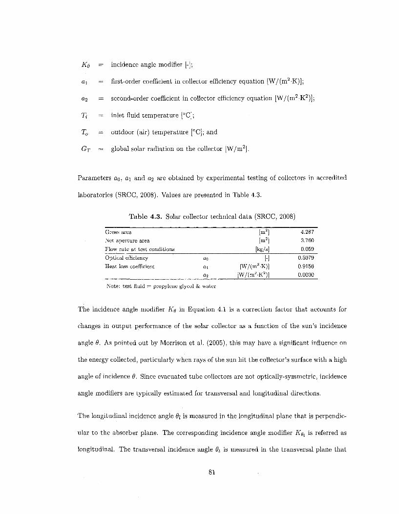
KQ = incidence angle modifier [-];
a\ = first-order coefficient in collector efficiency equation [W/(m2 •!<)];
a,2 = second-order coefficient in collector efficiency equation [W/(m2-K2)];
Ti = inlet fluid temperature [°C];
T0 = outdoor (air) temperature [°C]; and
GT = global solar radiation on the collector [W/m2].
Parameters ao, aj and ai are obtained by experimental testing of collectors in accredited
laboratories (SRCC, 2008). Values are presented in Table 4.3.
Table 4.3. Solar collector technical data (SRCC, 2008)
Gross area
Net aperture area
Flow rate at test conditions
Optical efficiency
Heat loss coefficient
ao
ax
ai
[m2]
[m2]
[kg/s]
H [W/(m2.K)]
[W/(m2-K2)]
4.287
3.760
0.059
0.5079
0.9156
0.0030
Note: test fluid = propylene glycol & water
The incidence angle modifier KQ in Equation 4.1 is a correction factor that accounts for
changes in output performance of the solar collector as a function of the sun's incidence
angle 9. As pointed out by Morrison et al. (2005), this may have a significant influence on
the energy collected, particularly when rays of the sun hit the collector's surface with a high
angle of incidence 9. Since evacuated tube collectors are not optically-symmetric, incidence
angle modifiers are typically estimated for transversal and longitudinal directions.
The longitudinal incidence angle 9\ is measured in the longitudinal plane that is perpendic
ular to the absorber plane. The corresponding incidence angle modifier Kgl is referred as
longitudinal. The transversal incidence angle 9t is measured in the transversal plane that
81

is perpendicular to the collector absorber and the longitudinal plane. The corresponding
incidence angle modifier Ket is referred as transversal. As shown in Figure 4.4, the collector
test report (SRCC, 2008) provides values of Kgt for different dt (at 0; = 0) and Kgt for
different &i (at 9t = 0). These data are set in an input file. Then, the model approximates
the incidence angle modifier KQ for any 9[ and B\ by multiplying K^p and Kotot.
1,20 -j —
I.IO 4
1.00
0.90 1 ~
transversal
longitudinal
r g 0.70
c 0.60 r £ 0.40
0.30
0.20
0.10 0.00 -' s i • ; ': ) f i
0 10 20 30 40 50 60 70 80 90
Angle & [°]
Figure 4.4. Incidence angle modifiers based on SRCC (2008) test results
As an example and in order to illustrate the performance of the collector, the solar
collector thermal efficiency for three different weather conditions are calculated based
on Equation 4.1, assuming Ke equal to 1 (Figure 4.5). If the temperature difference
T{ — T0 = 50°C, the collector efficiency is about 31% on a clear day and 9% on a cloudy
day.
82

iTrT0)l'C]
- • -C lea r day
# Mildly cloudy
-* -Cloudy day
100
Figure 4.5. Solar collector efficiency
Type 538 requires additional informations to apply analytical corrections to the ideal
efficiency curve to account for operating at flow rates other than values at test conditions
and for the number of identical collectors mounted in series. Yet, these corrections required
linear efficiency curves and Equation 4.1 is converted as:
Qv ACGT
FR(Ta)nK0-FRU'L(Ti To)
Gf (4.2)
where:
Ac
GT
FR
= useful energy gain [W];
= total collector array (gross) area [m2];
= global solar radiation on the collector [W/m2];
= overall collector heat removal efficiency factor [-];
83
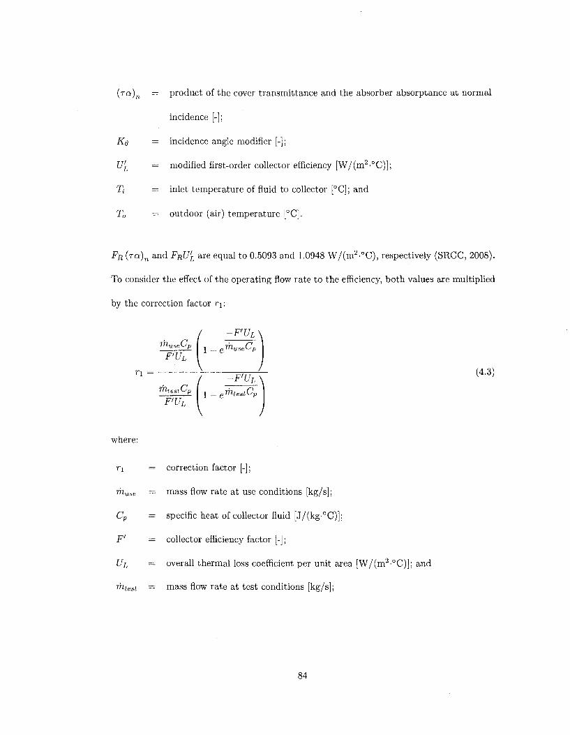
{ra)n — product of the cover t ransmit tance and the absorber absorptance at normal
incidence [-];
KQ = incidence angle modifier [-];
U'L = modified first-order collector efficiency [W/(m 2 ' °C)] ;
% = inlet temperature of fluid to collector [°C]; and
T0 = outdoor (air) temperature [°C].
FR (To) n and FRU'L are equal to 0.5093 and 1.0948 W/(m 2 - °C) , respectively (SRCC, 2008).
To consider the effect of the operating flow rate to the efficiency, both values are multiplied
by the correction factor r\:
-F'UL
F'UL
|_ „_ g 'i^use^p
n = ) - W (43)
^ ^ P i _ erhtestCp F'UL
where:
r\ = correction factor [-];
rhuse — mass flow rate at use conditions [kg/s];
Cp = specific heat of collector fluid [J/(kg-°C)];
F' = collector efficiency factor [-];
UL = overall thermal loss coefficient per unit area [W/(m2-°C)]; and
rhtest = mass flow rate at test conditions [kg/s];
84

The value of F'UL is calculated at test conditions:
F>UL = - ^ # In (l - F R U ' ^ ) (4.4) Ac \ mtestCp )
For instance, if the operating flow rate is 0.03 kg/s and the flow rate at test conditions is
0.059 kg/s (Table 4.3), the correction factor r\ equals 0.994.
To consider the number of identical collectors mounted in series Ns, a second correction
factor r2 multiplies FR(ra)n and FRU'L:
1 _ | ! _ A°F*U± i \ Ns
r2 = —- 7;;ir (4.5)
For instance, if the operating flow rate is 0.03 kg/s and four collectors are mounted in series
(Ns = 4), thenr2 = 0.965.
Thermophysical properties of the fluid
The solar collector's manufacturer recommends the use of propylene glycol as antifreeze
solution, with concentrations from 0 to 70% (Viessmann, 2008). Since the freezing
temperature is a direct function of the concentration, it has to be selected carefully in
order to avoid damages to the collectors during cold months.
The freezing temperature Tp, expressed in [K], is as a function of polypropylene glycol
concentration £ (M. CONDE Engineering, 2002):
TF 1 n n W o « n , „ „ r n t 2
273.15 1 - 0.03736£ - 0.40050^ (4.6)
85

The concentration of antifreeze is set at 50% (Cruickshank and Harrison, 2006). Based on
Equation 4.6, this corresponds to a freezing temperature Tp of 240.7 K (-32.5°C) which is
way below the outdoor design dry-bulb temperature for heating recommended by ASHRAE
(2005) of 250.15 K (-23°C).
The thermophysical properties of the fluid are required in several TRNSYS components
such as pumps, pipes, heat exchangers and solar collectors. However, these values can
only be set as fixed parameters and not as input variables, which implies that an average
operating temperature needs to be assumed.
The density, specific heat and thermal conductivity are calculated in terms of glycol's
concentration £ and the average operating temperature T. Each property is represented
by Px (M. CONDE Engineering, 2002), as follows:
, , , 273.15 . ,273.15 . /273.15\ 2 ,„ „. Px = Al+A2( + A3-jr- + A^~^- + A5(-jr-J (4.7)
The computation of the dynamic viscosity fi is performed using a sightly different
expression (M. CONDE Engineering, 2002), as follows:
i / \ A A * A 273.15 , ,273.15 , /273.15\ 2 /ia.
ln(At) = Ax + A2i + Az—jr- + A ^ - ^ — + A5 ( — j r - ) (4-8)
The value of parameters A\t A2, A3, A4 and A$ are presented in Appendix D. The resulting
density, specific heat, thermal conductivity and dynamic viscosity are illustrated from
Figures 4.6 to 4.9.
86

1070
-30 -20 -10 10 20 30 40 50 60 70 80 90 100
Temperature [°C]
Figure 4.6. Variation of density of propylene glycol with temperature
Figure 4.7. Variation of specific heat of propylene glycol with temperature
87

-30 -20 -10 10 20 30 40 50 60 70 80 90 100
Temperature [°C]
Figure 4.8. Variation of thermal conductivity of propylene glycol with temperature
Figure 4.9. Variation of dynamic viscosity of propylene glycol with temperature

The density and specific heat curves vary almost linearly with the operating temperature
(Figures 4.6 and 4.7). The dynamic viscosity and thermal conductivity, however, present
a different trend (Figure 4.8 and Figure 4.9). The average operating temperature of
the antifreeze is assumed at 80° C, which corresponds to the average temperature of
the antifreeze in the collector as calculated by the computer model. The corresponding
thermophysical properties used further in this study are shown in Table 4.6.
Table 4.6. Thermophysical properties of glycol used in the study
p [kg/m3]
990
Op
[kJ/(kg.°C)]
3.746
A
[W/(m.°C)]
0.384
P [Pa-s]
0.00087
TF
l°C] -32.5
Piping between collectors and storage
Two Types 709, one for cold side and one for hot side, are used to model copper pipes
between solar collectors and the water tank. Each pipe is divided in three segments to
represent the transit of the fluid through the attic, first floor and basement. So, the indoor
air temperature is set as input and the computed environment losses are established as
another source of heat gains in these three zones (Figure 4.2). Pipes length is approximated
at 10 m for the cold side and 10 m as well for the hot side. They are covered by a 40 mm
thick insulation material able to resist to high temperature, with a thermal conductivity of
0.04W/(m-°C).
In order to limit the hydraulic head, the flow velocity inside the copper pipes is between
0.4 m/s and 0.7 m/s (Viessmann, 2008). Therefore, the standard size is selected as a
function of the design flow rate and according to data provided in Table 4.7.
89

Table 4.7. Recommended dimensions of pipes. Prom Viessmann (2008).
Standard size [mm]
Outside diameter [mm]
Inside diameter [mm]
Plow rate (total
collector area)
H/h] 200
250
300
350
400
450
500
600
700
800
900
1000
1500
2000
2500
3000
12.7
15.9
13.4
15.9
19.1
16.6
19.1
22.2
18.9
Velocity of flow rate [m/s]
0,42
0.52
0.63
0.73
0.84
0.94
1.04
1.25
1.46
1.67
1.88
2.09
3.14
4.19
5.23
6.28
0.28
0.35
0.41
0.48
0.55
0.62
0.69
0.83
0.97
1.11
1.24
1.38
2.07
4.14
4.84
3.09
0.18
0.22
0.27
0.31
0.35
0.40
0.44
0.53
0.62
0.71
0.80
0.88
1.33
1.77
2.21
2.65
25.4
28.6
25.3
0.11
0.14
0.17
0.20
0.23
0.25
0.28
0.34
0.40
0.45
0.51
0.57
0.85
1.13
1.41
1.70
31.8
34.9
31.6
0.07
0.09
0.10
0.12
0.14
0.16
0.17
0.21
0.24
0.28
0.31
0.35
0.52
0.69
0.86
1.04
38.1
41.3
37.6
0.05
0.06
0.07
0.08
0.09
0.10 0.12
0.14
0.16
0.19
0.21
0.23
0.35
0.47
0.58
0.70
Type 534: Storage tank
The vertical cylindrical storage tank, installed on the basement floor, is developed using
Type 534 since it has the ability to model stratifiers (TESS, 2007). The tank diameter is
calculated based on its volume and its total height, which is assumed at 5.2 m, corresponding
to the cumulative height of the basement and the first floor.
The tank is divided into ten horizontal isothermal layers of equal volume (Figure 4.10) to
consider the stratification effect. A previous study (Braun et al., 1981) showed that ten
layers are sufficient to model accurately the stratification of a seasonal storage tank.
90
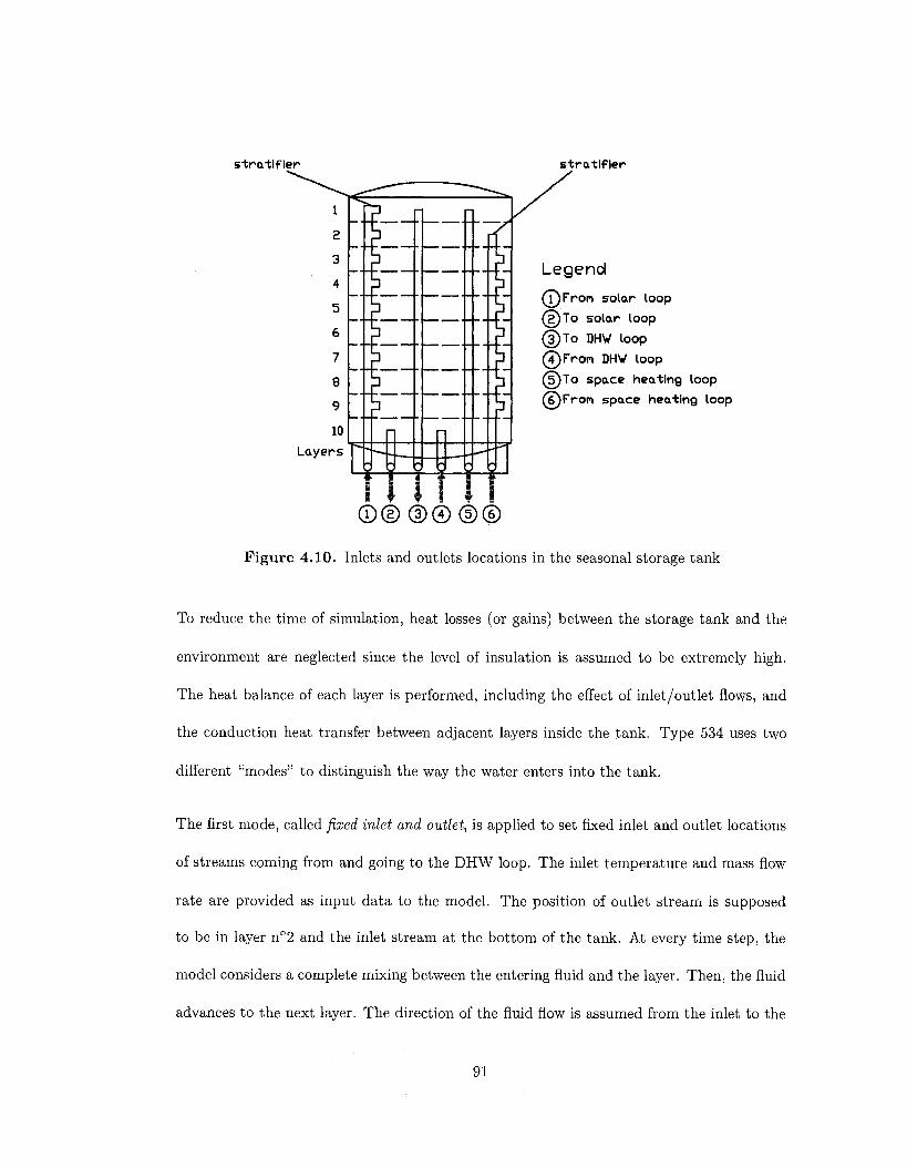
strat l f ler strat l f ler
^"-•^ 1
2
3
4
5
6
7
8
9
10
Layers
-F-
mm ®®®®®®
Legend
(T^Fropi solar loop
( D To solar loop
(5) To DHV loop
(4)From DHV loop
© T o space heating loop
( y F r o n space heating loop
Figure 4.10. Inlets and outlets locations in the seasonal storage tank
To reduce the time of simulation, heat losses (or gains) between the storage tank and the
environment are neglected since the level of insulation is assumed to be extremely high.
The heat balance of each layer is performed, including the effect of inlet/outlet flows, and
the conduction heat transfer between adjacent layers inside the tank. Type 534 uses two
different "modes" to distinguish the way the water enters into the tank.
The first mode, called fixed inlet and outlet, is applied to set fixed inlet and outlet locations
of streams coming from and going to the DHW loop. The inlet temperature and mass flow
rate are provided as input data to the model. The position of outlet stream is supposed
to be in layer n°2 and the inlet stream at the bottom of the tank. At every time step, the
model considers a complete mixing between the entering fluid and the layer. Then, the fluid
advances to the next layer. The direction of the fluid flow is assumed from the inlet to the
91

outlet layer. At any time, the temperature at the outlet equals the average temperature of
the layer containing it.
The second mode, called temperature seeking inlets with fixed outlets, is used to simulate the
effect of stratifier devices for the solar and heating loops. For each inlet, the temperature
and mass flow rate are provided as input data. Then, the model directs the water into the
layer closest in temperature to the incoming water temperature. The position for the radiant
heating floor is in layer n°l , and the outlet position for the solar loop is at the bottom of
the tank. With the inlet location knowns, the outlet temperature is then calculated as in
the first mode.
Type 656: Pumps
In the solar loop, two Type 656 components are used to model the variable speed pumps
that supply any mass flow rate up to the rated value (TESS, 2007). The pump starting
transient characteristics are not modeled.
The role of Solar pump n°l (point 2 in Figure 4.1) located on the primary loop is to circulate
the antifreeze solution from the solar collectors to the external solar heat exchanger. The
operating mass flow rate rhsoiar is directly proportional to the total solar collector area and
is chosen equal to 40 kg/(hrm2). The pump Wilo-Stratos ECO-ST from Wilo (2008) is
chosen. The rated power Prated is 40 W, the rated flow rate rhrated is 2,500 kg/h and the
maximum inlet fluid temperature is 110°C.
Based on the curve presented in the technical documentation, the electrical power input P
92

is modeled using a polynomial:
P = Prated (0.30 + 6.387 - 19.8772 + 31.1273 - I8.8874 + 1.9575) (4-9)
where:
P
* rated
7
electrical power [W];
rated power of the pump [W]; and
pump control signal [-].
The control signal of the pump 7 is:
Wlsolar
'Wlrated (4.10)
The electric power of the pump is illustrated in Figure 4.11.
0 0.1 0.2 0.3 0.4 0.5 0.6 0.7 0.8 0.9 1
Control signal y
Figure 4.11. Electric power of Solar pump n°l as a function of the control signal
93

The Solar pump n°2 (point 5 in Figure 4.1) circulates the hot water in the secondary loop
from the external solar heat exchanger to the storage tank. The operating mass flow rate
rhpump that is required to increase the temperature of water supplied to the tank to a
maximum of 95°C (Viessmann, 2008) needs to be estimated:
— ' c ^p,fluid (All") mpump ~ f^solar ' Qt- _ rp ' s-i Vi-'-'-i yo i j ^p,water
where:
rnpump — operating mass flow rate of the pump [kg/h];
^solar = mass flow rate of antifreeze coming from collectors [kg/h];
Toc — outlet temperature of collectors that is equal to the inlet temperature of
the pump [°C];
Tho = high temperature of fluid leaving the heat exchanger [°C];
Ttank,bottom — temperature at the bottom of the tank [°C];
Cpjiuid = specific heat of antifreeze [kJ/(kg-°C)]; and
CPtwater — specific heat of water [kJ/(kg-°C)].
The variable speed pump Wilo-Stratos ECO (Wilo, 2008) is selected and presents identical
technical proporties as Solar pump n°l . The control signal 7 is:
'"'rated (4.12)
External solar heat exchanger
Type 5 models the external cross flow heat exchanger (point 4 in Figure 4.1) required to
transfer the heat from the primary loop (hot side) where circulates the propylene glycol to
94

the secondary loop (cold side) where circulates water. Fluids are unmixed. The heat transfer
capacity rate of the heat exchanger is based on the correlation developed by Heimrath (2003)
in Task 26 (IEA SHC, 2007):
(UA)HX = (88.561AC + 328.19) (4.13)
where:
(UA)HX = heat transfer capacity rate [W/°C]; and
Ac = total collector array (gross) area [m2].
Control strategy
The control strategy of the solar loop is achieved with three Type 2 controllers. The
first controller (In-OutQ) checks if the collectors outlet temperature is higher than the
temperature at the bottom of the tank, with an upper and lower dead band equals to
10°C and 3°C, respectively (Heimrath, 2003). The second controller (TmaxPump) checks
if the collectors outlet temperature is lower than 110°C to avoid damaging the Solar pump
n°l (Wilo, 2008). Finally, the third controller (TmaxTank) checks if the temperature inside
the tank is lower than 95°C (Viessmann, 2008).
A solar control unit, modeled with a calculator, starts the Solar pump n°l when all the
controllers output are equal to 1, at the same time. Solar pump n°2 is turned on when
In-OutQ and TmaxTank output are equal to 1.
4 .3 .2 S p a c e h e a t i n g
The components used to model the radiant floor heating system are presented in Figure 4.12.
95

"HjpP Tyj>e534
I p -
• » - * -
Typellh 'V
Rad floor
Type23
Typellb
>
Type659-2
-^K
Heating pump
Type647 • _ | J
Type649
Tsetpoint-heat
Figure 4.12. TRNSYS components used to model the heating loop
Radiant floor
For modelling the radiant heating floor, an "active layer" is added to floor definition in
Type 56 (multizone building). The layer is called "active" because it contains fluid filled
pipes that either add or remove heat from the surface. Parameters used to define active
layers are the pipe spacing (10 cm), pipe outside diameter (2 cm), pipe wall thickness
(0.2 cm) and PEX pipe wall conductivity (0.35 W/m-°C) (Liu et al., 2000). Also, the
number of fluid loops is set at 10 for each floor. This is used for calculating the pipe length,
as:
pipe length = — floor surface area
pipe spacing • number of loops
96
(4.14)
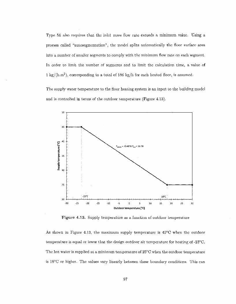
Type 56 also requires that the inlet mass flow rate exceeds a minimum value. Using a
process called "autosegmentation", the model splits automatically the floor surface area
into a number of smaller segments to comply with the minimum flow rate on each segment.
In order to limit the number of segments and to limit the calculation time, a value of
1 kg/(h.m2), corresponding to a total of 186 kg/h for each heated floor, is assumed.
The supply water temperature to the floor heating system is an input to the building model
and is controlled in terms of the outdoor temperature (Figure 4.13).
3 U -
r-* 40 '
3
E <u a. 35 • E 01
> a. OL 3
"" 30 •
25 -
20 - i i i i
,
; -23-C 1 ' • * ' ' 1 •' ' ' ' 1 '
^ V iupply ~
' i ' i ' .i i i i i '
-0.4878 Tm,+ 33.78
' ' 1 | i i, . . . |
18T • ' ' i I i i r , 1 i i i i 1 i , i i
-30 -25 -20 -15 -10 -5 0 5 10 15 20 25 30
Outdoor temperature [°CJ
Figure 4.13. Supply temperature as a function of outdoor temperature
As shown in Figure 4.13, the maximum supply temperature is 45°C when the outdoor
temperature is equal or lower that the design outdoor air temperature for heating of -23°C.
The hot water is supplied at a minimum temperature of 25°C when the outdoor temperature
is 18°C or higher. The values vary linearly between these boundary conditions. This can
97

be expressed as:
Tsuppiy = -0.4878 • T0 + 33.78 (4.15)
Using an Equation-Type (calculator), the final supply temperature is defined as the
maximum temperature between the temperature calculated in Equation 4.15 and the return
temperature given by Type 56. This value is then sent back to Type 56 as input data.
Control strategy
Type 23 is used to model a Proportional, Integral and Derivative (PID) controller that
adjusts the pump flow rate, in order to maintain the operative temperature on the first
floor at the setpoint of 20°C. That temperature, calculated by Type 56, is defined as input
data in Type 23. The value of the calculated flow rate rhCaic is between the rated flow rate
of the pump and the minimum inlet flow rate (186 kg/h). The remaining parameters of the
model such as the gain constant, integral and derivative time are selected equal to 744, 8 h
and 0.5 h, respectively.
To ensure that the supply water temperature Tsuppiy complies with Equation 4.15, a
tempering valve is modeled (Type lib) to adjusts the amount of return fluid that "bypasses"
the storage tank (point 11 in Figure 4.1). The bypassed return water is mixed with water
coming from the hot source by a tee piece (Type l lh).
Tankless water heater
Type 659-2 models the tankless water heater used to boost the temperature of hot water
for space heating if necessary. The 15 kW Eemax Series Two (Eemax, 2008) electric water
98

heater is chosen. The thermal losses are not considered and its efficiency is assumed at
100%. The device is turned on if the temperature of water coming from Type l l h is lower
than the calculated value in Equation 4.15, and if the operative temperature (controlled by
the Type 2 AuxHeaton) on the first floor goes below 20°C. The auxiliary energy transmitted
to the fluid by the heating element is:
(°£aux ~ TT^calc^p^water {-'•supply •'•%) v*-^-™)
where:
Qaux = auxiliary energy added to the fluid by the heater [kJ/h];
locale = fl°w r a t e calculated by Type 23 [kg/h];
CPtwater = specific heat of water [kJ/(kg-°C)];
Tgupply = temperature of hot water calculated in Equation 4.15 [°C]; and
Tj = temperature of water coming from Type l l h [°C].
Heat distribution
Like the Solar pump n°2, the Wilo-Stratos ECO is selected as the variable speed pump for
the radiant floors (point 12 in Figure 4.1). The rated power Prated is 40 W and the rated
flow rate fnrated is 2,500 kg/h. During the heating season, from October 1 to May 15, the
control signal of the pump 7 is:
7 = (4.17) TW>rated
where:
99

7 = pump control signal [-];
i^calc — n o w r a te calculated by Type 23 [kg/h]; and
^rated — rated flow rate [kg/h].
During the rest of the year, the pump is turned off and 7 equals 0. The electrical power
input is modeled using Equation 4.9.
Using Type 647, the water flow rate is then split to delivers hot water to the basement and
first floors, while Type 649 collects the return water and send it back to the storage tank
(Figure 4.12).
4.3.3 Domestic hot water
The components used to model the preparation of domestic hot water are presented in
Figure 4.14.
"iiifr
Type534
* <
DHW pump
DHWHX
- « • . ri - « « .
. j ^ mm DHW DHW data
l> Type65E>
Figure 4.14. TRNSYS components used to model the DHW loop
100

DHW pump
The variable speed DHW pump (Wilo-Stratos ECO) (point 7 in Figure 4.1) circulates the
hot water on the primary loop of the DHW external heat exchanger (point 8 in Figure 4.1).
The operating water flow rate rhpump that is required to increase the water temperature
from the city line to 45°C at the user-end is computed as:
rripump = rnDHw • T _ ™tv (4-18)
where:
rhpump — operating water mass flow rate of the pump [kg/h];
rhDHW — domestic hot water consumption from the given profile [kg/h];
Tdty = city line water temperature [°C];
Thi = temperature of hot water coming from the tank [°C]; and
Th0 = temperature of water going back to the tank [°C].
The control signal of the pump equals the ratio of the calculated operating flow rate to the
rated flow rate (Equation 4.12).
External DHW heat exchanger
Type 5 models the external cross flow heat exchanger (point 8 in Figure 4.1) used to transfer
the heat from the hot water coming out of the solar tank (hot side) to the water from the city
line (cold side). Fluids are unmixed. Based on the results of a parameters identification
process (Bales and Persson, 2003) and considering the hot water load profile, the heat
transfer coefficient of the heat exchanger (UA)HX is set to 6190 W/°C.
101

Tankless water heater
Type 659 models the 15 kW Eemax "Series Two" (Eemax, 2008) tankless water heater used
to boost the temperature of domestic hot water if necessary. The device is turned on if the
temperature of water coming from the external heat exchanger is lower than 45° C. The
auxiliary energy transmitted to the fluid by the heating element is:
Qaux = mDHwCp<water ( 4 5 - Ti) ( 4 ' 1 9 )
where:
Qaux — auxiliary energy added to the fluid by the heater [kJ/hj;
riiDHW = domestic hot water consumption from the given profile [kg/h];
= specific heat of water [kJ/(kg-°C)]; and
Ti — temperature of water coming from the external heat exchanger [°C].
4.4 Preliminary design method
In the following section, a preliminary design method developed by Braun et al. (1981)
is used to predict the storage tank volume required to achieve heating and DHW needs
without any auxiliary heating source. This methodology is compared with the TRNSYS
results for storage volume to collector area ratios greater than 200 1/m2.
Since the s torage t ank is very large, the inside water t e m p e r a t u r e is not expected to vary
throughout each month, so an average collector inlet temperature is assumed. Consequently,
the utilizability (4>) method developed by Duffie and Beckman (2006) is used.
102

4.4.1 System description and simulation model
The schematic of the closed-loop space heating system with sensible storage is shown in
Figure 4.15. Solar energy Qu is collected and transmitted to a water storage tank through
an external heat exchanger. The primary source for heating and domestic hot water is the
energy supplied Qsupplied from storage. The tank is assumed very well insulated and the
heat losses are not considered. The water in the tank is supposed to be fully-mixed and,
therefore, the stratification is not considered. The return temperature from the heating
and domestic hot water loads is always at or above Tmjn. A bypass valve makes sure that
the temperature coming from the heat exchanger is always at or below Tg. An auxiliary
heating element covers the additional energy demand QaUx, if necessary. An energy balance
Storage tank AU
Energy supplied Qs
Auxiliary energy
Heating & DHW loads
a
Figure 4.15. Schematic of a closed-loop space heating system (Braun et al., 1981)
on the tank for a one-month period is performed, as:
ISU LJU y supplied (4.20)
where:
103

/\U = monthly change in internal energy of storage [GJ];
Qu = useful energy gain [GJ]; and
Qsupplied — energy supplied by the storage tank [GJ].
The radiation level must exceed a critical value before useful output is produced. This
critical level is expressed as follows:
FRU'L (Tt - Td0) lT° ~ FR(ra)- ( 4 2 1 )
where:
ITC — monthly critical level radiation [W/m 2 ] ;
FR = overall collector heat removal efficiency factor [-];
U'L — modified first-order collector efficiency [W/(m2-°C)];
( ra) n = product of the cover transmittance and the absorber absorptance at normal
incidence [-];
Tt = monthly average tank temperature [°C]; and
Tdo = monthly average daytime outdoor temperature [°C].
The daily utilizability <f> is calculated using the correlation method developed by Dume
and Beckman (2006). The useful energy gain of collectors NY2Qw characterized as the
difference between the absorbed radiation and the radiation losses to the surroundings over
a time period is calculated over each month:
N £ Qu = ^ACGTFRJ^O) (4.22)
104

where:
N = number of days in the month [-];
Qu = monthly average of daily useful energy gain [GJ];
cj) = daily utilizability [-];
Ac = total collector array (gross) area [m2];
GT = global solar radiation on the collector [W/m2];
FR — overall collector heat removal efficiency factor [-]; and
(ra) = monthly average product of the cover transmittance and the absorber
absorptance [-]; assumed equal to 0.96 (Duffle and Beckman, 2006).
The energy supplied to the load from storage QSUpplied 1S assumed to be the minimum of
the loads Qioads a n d the quantity of energy that could be supplied if the heat exchanger
operates continuously throughout the month:
Qsupphed = min (eCm i n (TT - TR) At,Qioads) (4.23)
where:
Qsupplied — energy supplied by the storage tank [GJ];
zCmin — product of the effectiveness of the heat exchanger and the minimum
capacitance rate of the heat exchanger [W/°C];
Tt = monthly average tank temperature [°C];
TR = room temperature [°C];
At = length of time in the month [s]; and
Qioads = sum of space heating and domestic hot water loads [GJ].
105

The eCmin product is selected to respect the following condition (Braun et al , 1981);
0.4 < (TfA™n < 2 (4.24) \U A)house
where (UA)house is the overall loss conductance of the "best case" house.
The annual solar fraction of the solar combisystem is finally computed as:
/
year
Qaux dt
year Qloads d t
(4.25)
where:
& = annual solar fraction [-];
Qaux = auxiliary energy [GJ]; and
Qloads — s u m 0 I space heating and domestic hot water loads [GJ].
Since Qioads is equal to the sum of the energy supplied by the storage tank Qsupplied a n d
Qaux, Equation 4.25 is rewritten as:
/
year
Qsdt •r = -Jyear (4-26)
Qloads d*
4.4.2 Methodology
Given an initial storage tank temperature 7\ at the start of the month of March, for example,
the average temperature of the same month Tt is guessed. The final tank temperature at
106

the end of the month is given by:
Tf = 2-Tt-Ti (4.27)
Tt is used to calculate the critical radiation level 7j-c (Equation 4.21) and the resulting
utilizability <$>. The tank energy balance is then applied to estimate the tank temperature
at the end of the month:
Tf = — + Ti = Qu Qsu™lied + T% (4.28) caps caps
The thermal capacitance of the storage medium caps, expressed in GJ/°C, is:
caPs = Vt-p-Cp (4.29)
where:
Vt — volume of the tank [m3];
p = density [kg/m3]; and
Cp = specific heat [GJ/(kg-°C)].
This calculated temperature is compared with the assumed value (Equation 4.27), and if
they agree, the computation continues with the next month. If the temperature difference
exceeds 0.1°C, another monthly average temperature is estimated and a new final tank
temperature is calculated until the agreement is reached between the guessed value of Tt
and the calculated value. The process is repeated for all twelve months, and the final tank
temperature Tf is compared with the initial guess made for March. If they agree, the
107

calculations are stopped; if they disagree, the calculations are repeated.
4.4.3 Input data
An array of twelve identical Vitosol 300 SP3 solar collectors is assumed to cover as much as
possible the area on the south part of the roof. The resulting absorber surface area is equal
to 51.4 m2. Meteorological, outdoor temperature and solar radiation data are extracted
from the weather file used by TRNSYS. The parameters used for the preliminary design
method are presented in Table 4.21.
Table 4.21. Parameters used in the preliminary design method
Solar collector _ _ _ ——
FR (ra)n [-] 0.5093 FRU'L [W/(m2 .°C)] 1.0948 Tilt angle [°] 45 Orientation [-] South TB [°C] 95 Load
(UA)L
TR
[W/°C]
[°C]
120
20
Load heat exchanger
dsrnin
•*• min
[W/°C]
[°C]
168
25
Thermal storage
Medium
Op
p
[-]
[kJ/(kg.°C)]
[kg/m3]
Water
4.19
1000
4.4.4 Results
For a total collector area of 51.4 m2, the annual solar fraction of 100%, synonym of a seasonal
storage system, is achieved when the tank volume comes close to 38,600 1 (Figure 4.16).
The ratio of the tank volume to the collector area is equal to 750 1/m2.
108

1.00
0.95 H
0.50
10,000 15,000 20,000 25,000 30,000
Storage Volume [i]
35,000 40,000
Figure 4.16. Solar fraction as a function of the storage volume
4.5 TRNSYS simulation results and discussion
This section presents the TRNSYS simulation results for the seasonal storage system
associated with a hydronic radiant heating floor and domestic hot water, as described
previously. The model runs over two years since initial temperature of the storage tank is
unknown. Therefore, each layer is assumed at a temperature of 60°C at the beginning of
the first year. Results at the end of the first year are input as initial conditions for the
simulation of the second year. Since the first year of operation is not representative, only
the results of the second year are presented.
Using information available for the domestic hot water consumption profile (Jordan and
Vajen, 2001), the simulation time step is reduced to six minutes in order to provide a more
109

realistic representation of temperature variation inside the tank. The flow rate of the Solar
pump n°l is fixed at 40 kg/(h-m2).
4.5.1 Overall performance
According to the TRNSYS simulation results, the total house electricity use is equal to
8,300 kWh (29,880 MJ), corresponding to 45 kWh/m2 (161 MJ/m2) of heated floor area.
Compared to the total eletricity use of 18,830 kWh of the "best case" (without solar energy),
this represents a drastic decrease as the total energy use is divided by a factor bigger than
2.
The monthly repartition of electricity use during the year as well as its distribution among
end-uses are shown in Table 4.22. The Heating & DHW part represents the eletricity use
due to the circulating pumps. The winter months have the highest contribution to the
consumption due mainly to the ventilation system since the outdoor air needs to be heated
up to the temperature of 20°C. During summer, the months of July and August present
higher demand as a result of the cooling system.
Table 4.22. Monthly repartition and distribution of electricity use
Electricity use Month
[kWh] Jan Feb Mar Apr May Jun Jul Aug Sep Oct Nov Dec Tot
Heating & DHW 24~ 24~ 29 20 1 V T 2 1 4 18 21 150~
Humidiflcation 205 173 125 37 1 - 4 51 167 764
Cooling - - - 7 146 310 231 47 740
Lighting 133 108 102 88 72 65 68 81 96 121 141 146 1,220
Ventilation 670 593 590 469 347 285 294 294 285 429 523 642 5,421
Total 1,035 900 846 613 432 498 673 608 429 558 732 976 8,300
Figure 4.17 presents a comparison between the monthly electricity use in the base case and
the solar combisystem. It shows a drastic decrease from April to October. However, the
difference is less sensible during the period where the heating system is turned off.
110
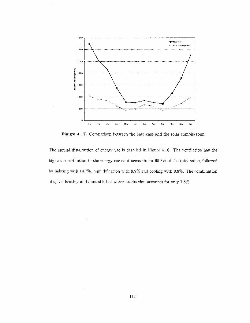
2,500
E1
£ 2,000 us
e ric
ity
3
K " J w
Ele
1,000 •
o •
\ - • - B a s e case
-fe Solar combisystem
\ / \T \
V \ \
\ \
\-_«_-^---***~~-. B
/ •/*'"* * ~* ••""
Jan Feb Mar Apr May Jun Jul Aug Sep Oct Nov Dec
Figure 4.17. Comparison between the base case and the solar combisystem
The annual distribution of energy use is detailed in Figure 4.18. The ventilation has the
highest contribution to the energy use as it accounts for 65.3% of the total value, followed
by lighting with 14.7%, humidification with 9.2% and cooling with 8.9%. The combination
of space heating and domestic hot water production accounts for only 1.8%.
I l l

Lighting 14.7% (1,220 kWh
Humidification 9.2% (764 kWh)
Cooling 1.9% (740 kWh)
Heating & DHW .1.8% (150 kWh)
Ventilation 65.3% (5,421 kWh)
Figure 4.18. Annual distribution of electricity use
The monthly average operative temperature of the first floor is shown in Figure 4.19. During
the cooling season, the cooling system is able to maintain the temperature around 24°C.
During the heating season, the temperature is systematically above the design setpoint of
20° C by approximately 0.5°C.
112

Jan Feb Mar Apr May Jun Jul Aug Sep Oct Nov Dec
Figure 4.19. Monthly average of operative temperature
This overheating phenomenon is very well illustrated in Figure 4.20 for the first three days of
February since the operative temperature goes up to a maximum of 23.5°C in the afternoon
of February 2.
Higher temperatures observed on February 2 can be seen as the direct result of exterior
conditions since the outdoor temperature and horizontal solar radiation present superior
values that particular day (Figure 4.21).
113

Day
Figure 4.20. Operative temperature in February
Day
Figure 4.21. Horizontal solar radiation and outdoor temperature
114

The surface temperature of the first floor is investigated in order to see if values comply with
allowable range of 19 and 29° C proposed by ASHRAE (2004). The minimum temperature
observed is 20°C and the maximum 28°C. Hence, the condition is well respected.
y j — 91 i~ =J
rat
0)
a E |S
29 -
28 -
27 -
26 -
25 -
24 -
23 -
22 -
0 730 1460 2190 2920 3650 4380 5110 5840 6570 7300 8030 8760
Time [h]
Figure 4.22. Inside surface temperature on the first floor
4.5.2 Performance of the solar combisystem
The following sections present the performance analysis of the seasonal storage system as
well as its various components, based on the TRNSYS simulation.
Storage tank
For indication only, the top layer, bottom layer and average tank temperatures are presented
during the first year of operation (Figure 4.23). The bottom and average temperatures drop
drastically during the first part of January. In the middle of February, the top temperature
starts to go up until the top layer reaches its maximum of 95° C. That temperature is
115

maintained until the end of November. However, the average and bottom tank temperatures
starts to drop in the middle of October due to a higher heating demand. It is observed that
the top layer temperature falls consequently one month and a half later, in December.
The temperature profile for the second year of operation (Figure 4.24) presents similarities
with the previous chart. The minimum temperature of the top layer occurs at the end of
January and is approximately 46-47°C. Since the hot water supplied to the radiant floor
is extracted from the top layer (Figure 4.10), this suggests that the combisystem may be
properly sized as the temperature is higher, but not significantly, than the maximum supply
temperature for space heating of 45°C (Figure 4.13).
116
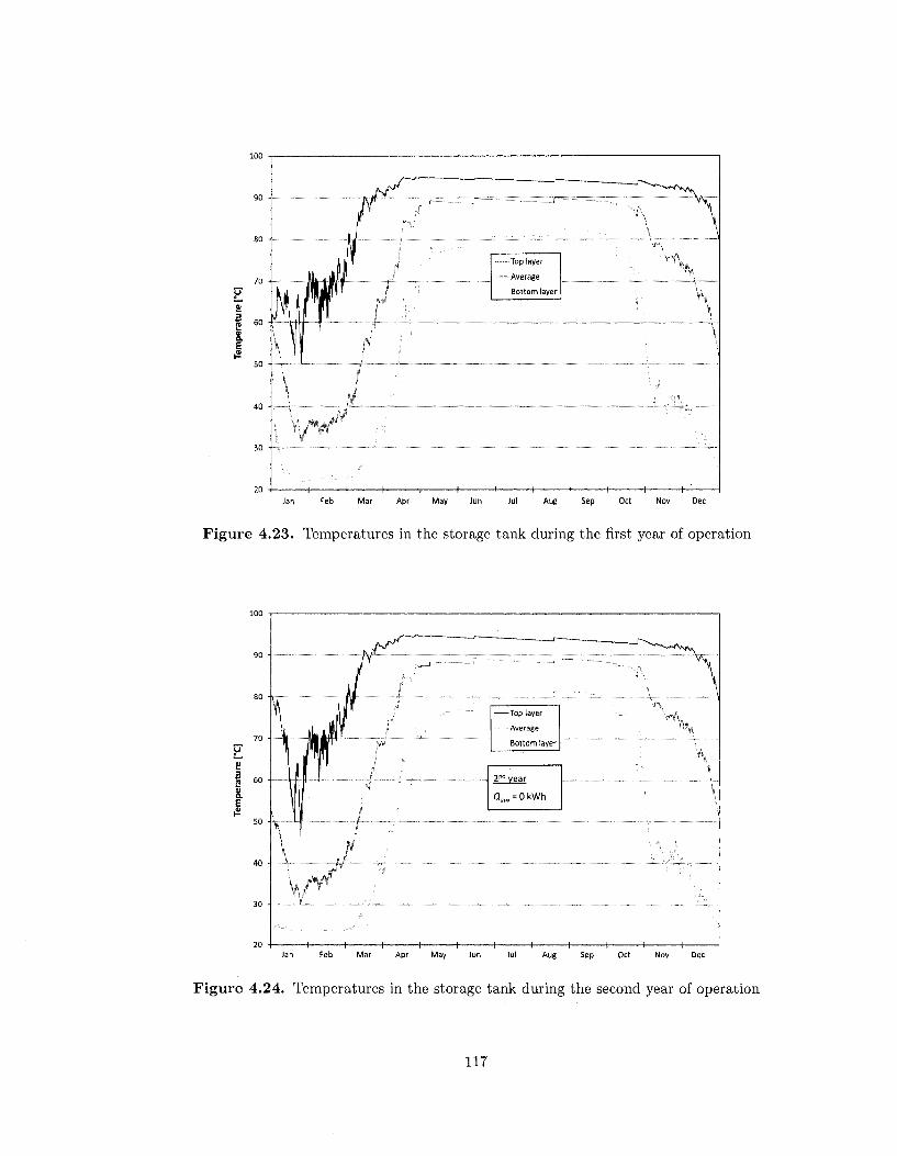
2L E
Top layer
Average
Bottom layer
1 1 1 1 1 1 h™ H r- ~ h - h
Jan Feb Mar Apr May Jun Jul Aug Sep Oct Nov Dec
Figure 4.23. Temperatures in the storage tank during the first year of operation
• f , '
If J
III Jl' ** . i In i
•v ••
X •I
III ? r! £f
* ^ *̂
ft # '
k
— \ 1 1 1 1
Top layer
Average
Bottom layer
2nd vear
Qoux = 0kWh
H 1
\
i, ^
r
1!
'1
—1 1 1 1 Jan Feb Mar Apr May Jun Jul Aug Sep Oct Nov Dec
Figure 4.24. Temperatures in the storage tank during the second year of operation
117

The profile of average tank temperature is illustrated in Figure 4.25 on a monthly basis.
Minimum values are noticed in January and February. During summer months, the
temperature comes close to 95° C, which is a sign that the input of solar energy coming
from the collectors maybe too elevated.
a E
• • • • •
rt
Jan Feb Mar Apr May Jun Jul Aug Sep Oct Nov Dec
Figure 4.25. Monthly average water temperature in the storage tank
Pumps
The time of operation and average mass flow rate of pumps are shown in Table 4.23. The
pumps are turned on mainly during the heating season to supply higher heating and DHW
demands.
118

Table 4.23. Time of operation and average mass flow rate of pumps
Time of operation
[h] Solar pump n°l
Solar pump n°2
Pump for heating
Pump for DHW
Mass flow rate
[kg/h]
Solar pump n°2
Pump for heating
Pump for DHW
Jan
219
167
199
15
Jan
82
436
76
Feb
248
201
144
13
Feb
96
457
43
Mar
315
245
124
15
Mar
121
405
36
Apr
212
164
69
12
Apr
181
345
31
May
61
35
4
10
May
382
307
27
Month
Jun
26
14
-11
Jul
16
6
-9
Month
Jun
1,023
-26
Jul
2,077
-22
Aug
26
11
-9
Aug
1,401
-20
Sep
12
5
-13
Sep
2,208
-23
Oct
28
17
52
15
Oct
670
311
26
Nov
155
111
170
12
Nov
78
344
30
Dec
170 121
213
16
Dec
81
397
36
The mass flow rate of Solar pump n°l is not presented as it remains constant at 40 kg/m2 of
collector area. From November to April, the monthly average mass flow rate of Solar pump
n°2 fluctuates between 78 and 181 kg/h (Figure 4.26). During the period when the average
tank temperature comes closer to 95°C (Figure 4.25), the values are increased substantially
up to a maximum of 2,208 kg/h in September. These high values could have negative impact
on the stratifiers performance since the flow rates are higher than 8 kg/min or 480 kg/h
(see Chapter 2).
The flow rate profile of the pump for space heating presents less variations, as values range
between 307 and 457 kg/h (Figure 4.27). The mass flow rate is directly related to the
heating demand, as higher values are observed during colder months, and to the supply
water temperature, which has higher values during the cold days.
Mass flow rates of variable speed pump for domestic hot water is associated to the storage
tank temperature (Figure 4.25). Indeed, as the temperature is low, the mass flow rate is
increased to ensure a 45°C hot water at the user end at all times (Figure 4.28).
119

2000
3 5
•—
-—•-
1
1
_. . j
1
1
I
1
1
1
1
1
1
- -
1
1 1 II
Jan Feb Mar Apr May Jun Jul Aug Sep Oct Nov Dec
Figure 4.26. Solar pump n°2 mass flow rates
•as a. 8oo
n 1
1 p
1 1
[.: ' 1 1 • 1 • 1 • 1 • 1
1 1
1
Jan Feb Mar Apr May Jun Jul Aug Sep Oct Nov Dec
Figure 4.27. Mass flow rates of the pump used for space heating
120

140 -
120 -
100 •
60 •
40 •
n •
1 1
1
- - - -
1
II <l
" " " „ '• " II... , . "
Jan Feb Mar Apr May Jun Jul Aug Sep Oct Nov Dec
Figure 4.28. Mass flow rates of the pump used for space DHW
Solar collectors
The outlet collectors temperature is presented on a monthly basis in Figure 4.29. The
average temperature oscillates between 65 and 85°C during the year. The maximum
temperature is limited to 110°C to avoid damaging the pump.
121

100 -
60 •
20 -
0 •
i
• • -•
*
l l> II
II
o
II
1
Jan Feb Mar Apr May Jun Jul Aug Sep Oct Nov Dec
Figure 4.29. Monthly outlet collectors temperature
The TRNSYS results show that the yearly average of the outlet temperature of collectors is
80°C and the corresponding inlet temperature is 76°C. Therefore, the average temperature
in the collectors is equal to 78°C, which corresponds to the initial guess of 80°C used to
estimate the thermophysical properties of the antifreeze.
The rate of useful energy gain of collectors is calculated by TRNSYS as:
Qu — fhCp (T0 — Ti, (4.30)
where:
y« —
m —
Cry —
Ti =
rate of useful energy gain [W];
the pump fluid flow rate through the collector [kg/s];
specific heat of collector fluid [J/(kg-°C)];
inlet temperature of fluid to collector [°C]; and
122

T0 — outlet temperature of fluid from collector [°C].
The rate of useful energy gain Qu is integrated over the second year is equal to 9,335 kWh.
4.5.3 Collection efficiency
A measure of collector performance is the collection efficiency T]TH, defined as the ratio of
the useful energy gain over a year to the incident solar energy on the collectors over the
same period (Duffle and Beckman, 2006):
/
year Qudt
VTH = JWaTr = 0.257 (4,31) Ac / GT dt
where:
TJTH = efficiency of collectors [-];
Qu = rate of useful energy gain [W];
Ac = total collector array (gross) area [m2]; and
GT = global solar radiation on the collector [W/m2],
If the electric energy use of pumps Qpumps is considered, the collection efficiency is:
/
year Qudt
'ITH+ELEC — Jyeay Tyear = 0.256 (4.32) Ac / GT dt+ Qpumps dt
123

4.5.4 Solar fraction
No auxiliary heating is required to provide additional heat in the storage tank during the
second year of operation. Therefore, the solar fraction of the system is:
/
year
tyaux " t
^TH = i - -pear = 1 (4-33)
/ Qloads dt
where:
&TH — annual solar fraction [-];
Qaux — energy supplied to the storage tank by the tankless water heaters [kWh]; and
Qloads — sum of space heating and hot water loads [kWh].
The solar fraction that considers the energy use of the circulating pumps is:
/
year
[Qaux T typumps) d t ^TH+ELEC - ryear = 0.975 (4.34)
Qloads dt
4.5.5 Coefficient of performance
The coefficient of performance (COP) of the solar combisystem is calculated using the
following equation:
/
year {Qheat + QDHW) dt
o w r = jyzsf = 49.3 (4.35) typumps d t
The energy supplied for space heating Qheat is calculated as:
Qheat — mheatCp (Tsupply — Tret) (4.36)
124

where:
Qheat = energy supplied for space heating [W];
reheat = mass flow rate of hot water supplied by the circulating pump [kg/s];
Cp = specific heat of water [J/(kg-°C)];
Tsupply = supplied temperature [°C]; and
Tret = return temperature [°C].
The energy supplied for domestic hot water preparation QDHW is calculated as:
QDHW = rriDHwCp (45 - Tcity) (4
where:
QDHW = energy supplied for domestic hot water preparation [W];
mDHW — domestic hot water consumption profile [kg/s];
Cp = specific heat of water [J/(kg-°C)]; and
Tdty — city line temperature [°C]; and
125

4.6 Sensitivity analysis
In this section, a sensitivity analysis based on a certain set of design parameters is performed
in order to evaluate the repercussions of those parameters on the seasonal storage system and
to improve its performance, A comparison between evacuated tube and flat-plate collectors
is presented. For each type of collectors, several alternatives are proposed based on the
parameters that are expected to have a significant impact. Modifications are investigated
on:
— storage tank volume;
— solar collector area;
— insulation of the storage tank;
— operating mass flow rate of Solar pump n°l;
— tilt angle.
4.6.1 Evacuated tube collectors
The solar combisystem described in previous sections is considered as the base case for the
sensitivity analysis.
Influence of the storage tank volume
The volume of the storage tank is reduced by 10, 20 and 30% to see the resulting performance
of the system. Compared to the base case, the alternative 1 has almost no impact as the
solar fraction remains close to 100% (Table 4.29). However, for alternatives 2 and 3, a
drastic decrease of performance occurs as the COP is divided by a factor 2 each time that
126

the tank volume is reduced by 10%. The collection efficiency remains constant around
25.4-25.8%.
Table 4.29. Performance of the solar combisytem for different storage tank volumes
Alternative
Base case
1
2
3
Volume
[m3]
38.6
34.7
30.9
27.0
f]TH
[%] 25.7
25.7
25.8
25.4
r]TH+ELBC
[%) 25.6
25.6
25.7
25.3
tyaux
[kWh]
-9
151
388
Vp-u mps
[kWh]
151
151
154
157
&TH
[%] 100.0
99.8
97.5
93.5
&TH+ELEC
[%] 97.5
97.3
94.9
90.8
COP
H 49.3
46.5
24.3
13.5
Influence of the solar collector area
The total area of collectors is reduced by substracting 1, 2 and 3 collectors. As shown in
Table 4.30, the fact to remove one element has almost no impact on the performance of the
system. However, for alternatives 2 and 3, the COP is divided approximately by a factor 2
each time that one collector is removed.
Table 4.30. Performance of the solar combisytem for different collector areas
Alternative
Base case
1
2
3
Area
[m2]
51.4
47.1
42.8
38.5
VTH
[%]
25.7
25.6
25.6
25.4
VTH+ELEC
[%] 25.6
25.4
25.5
25.2
tyaux
[kWh]
-5
82
307
typumps
[kWh]
151
159
168
180
&TH
[%] 100.0
99.9
98.6
94.8
&TH+ELEC
[%} 97.5
97.2
95.8
91.8
COP
H 49.3
45.3
29.6
15.1
Influence of the tank insulation
To give a more realistic perspective of the system, it is required to estimate the impact of
the storage tank heat losses to the environment. Therefore, a blanket of mineral wool with
a thickness 20 cm is assumed to cover the tank entirely. The resulting edge loss coefficient is
equal to 0.20 W/(m2-°C). That value, as well the air temperature of the surrounding space
127

(given by Type 56), are set as input in Type 534 for each of the tank layers. Reciprocally,
the tank losses are set as new heat gains in Type 56.
As presented in Table 4.31, the solar fraction of the system ^TH+ELEC is lowered by 5.7%.
The COP presents the most radical decrease as it drops from 49.3 to 12.8.
Table 4.31. Influence of the tank insulation on the performance of the solar combisystem
Alternative
Base case
1
TJTH
[%] 25.7
25.5
VTH+ELEC
{%}
25.6
25.4
(afaux
[kWh]
-
288
typumps
[kWh]
151
196
&TH
{%} 100.0
95.1
&TH+EIEC
[%] 97.5
91.8
COP
H 49.3
12.8
Since these results are more representative of a real system, it is decided to pursue the
sensitivity analysis using the alternative 1 (insulated tank) as the "new base case",
Influence of the operating mass flow rate of Solar pump n° 1
The mass flow rate of the thermal fluid circulating in the collectors rhsoiar is varied
between 25 and 51 kg/(h-m2). The minimum value corresponds to the minimum flow rate
recommended by the manufacturer to assure an appropriate circulation and a turbulent
flow in the collectors (Viessmann, 2008); and the maximum corresponds to the maximum
flow rate of Solar pump n°l (2,500 kg/h).
Table 4.32 shows that the alternative 1 lowers the energy use of the pumps since it is directly
proportional to the flow rate (Equation 4.9). Therefore, the solar fraction (^TH+ELEC) of
the base case is increased by 4% and the COP is almost doubled. Such system is preferred
as it also reduces the piping size (Table 4.7).
128

Table 4.32. Performance of the solar combisytem for different values of rhsoiar
Alternative
Base case
1
2
3
Flow rate
[kg/(h-m2)]
40
25
33
51
VTH
[%] 25.5
26.5
26.0
18.8
TfTH+ELEC
[%] 25.4
26.4
25.9
18.7
V a i i x
[kWh]
288
90
193
662
typumps
[kWh]
196
161
178
201
&TH
[%] 95.1
98.5
96.8
88.9
•^TH+ELBC
[%] 91.8
95.8
93.7
85.5
COP
H 12.8
24.3
16.5
7.3
Influence of the tilt angle
Four alternatives are proposed for the tilt angle. At 37.5°, the solar fraction ^TH+ELEC is
reduced by about 3.6% and the COP by 3.9 (Table 4.33). Then, by incrementing the tilt
angle by 7.5° up to 60°, the performance is clearly enhanced as the solar fraction comes
close to 95% and the COP to 20.
Table 4.33. Performance of the solar combisytem for different tilt angles
Alternative
Base case
1
2
3
4
Tilt angle
[°] 45.0
37.5
52.5
60.0
67.5
VTH
[%] 25.5
24.9
25.7
25.6
25.0
r\TH\ELEC
[%] 25.4
24.8
25.6
25.5
24.9
ictfaux
[kWh]
288
497
151
123
197
VpUTTlpS
[kWh]
196
204
192
191
202
&TH
[%] 95.1
91.6
97.5
97.9
96.7
^TH+ELEC
[%] 91.8
88.2
94.2
94.7
93.3
COP
H 12.8
8.9
18.0
19.6
15.5
129

Table 4.34 shows the monthly average temperature of the storage tank for the top layer
and the entire tank. On all cases, the lower temperatures occurs during the month of
January where the heating load is the most important (Table 3.6). During that month,
the maximum tank temperatures are observed for a tilt angle of 60°, which corresponds
precisely to the highest performances of the solar combisystem (Figures 4.30 and 4.31). For
its actual configuration, this implies that the system has to be designed to deliver high
temperatures in the storage tank during the "peak period" of heating loads, in order to
achieve greater solar fraction and COP values.
Table 4.34. Temperature in the storage tank for different tilt angles
Tilt angle Top layer temperature
[c] Jan Feb Mar Apr May Jun Jul Aug Sep Oct Nov Dec Year
37.5 33.2 38.8 71.8 88.4 86.6 80.5 83.5 84.7 83.7 77.9 75.0 68.3 72.9
45.0 38.4 44.7 78.3 89.0 85.9 82.3 85.6 82.2 84.0 82.0 77.2 71.6 75.3
52.5 42.4 47.4 79.4 88.7 87.4 84.0 84.6 82.5 84.9 82.9 79.1 74.2 76.6
60.0 43.3 54.8 82.0 89.1 86.2 84.1 82.8 83.0 84.1 81.8 77.8 73.6 77.0
67.5 40.8 55.2 81.7 88.3 84.8 82.3 82.2 82.4 86.0 82.1 77.1 74.1 76.5
Tilt angle Average temperature
[°] Jan Feb Mar Apr May Jun Jul Aug Sep Oct Nov Dec Year
37U 25T9 27\8 4L5 67~9 81~1 767 78̂ 2 787 7T9 72^6 6^2 48T 61.7
45.0 27.7 29.5 45.6 71.4 81.0 77.5 80.1 77.4 76.3 73.9 64.0 51.2 63.2
52.5 29.5 30.3 46.7 71.6 81.9 79.1 79.6 76.8 77.7 75.0 65.9 53.9 64.2
60.0 29.8 32.2 49.6 73.3 81.6 79.1 77.8 76.4 76.2 73.7 64.2 52.9 64.0
67.5 28.6 32.2 49.2 71.3 78.2 76.3 75.4 74.3 77.3 75.3 64.5 53.4 63.1
130

40
U 35
a E £> 30
V ' X ( ,,
-•If-Top layer
-•-Average
^ - ^ " ^ _
Tilt angle [°]
Figure 4.30. Variation of the storage tank temperature with the tilt angle during the month of January
50 55 60
Tilt angle [°]
80
Figure 4.31. Variation of T)TH+ELEC and the COP with the tilt angle
131

4.6.2 Flat-plate collectors
To consider the impact of flat-plate collectors on the solar combisystem, Type 538,
previously used to model the Vitosol 300 SP3 evacuated tubes solar collector, is replaced by
Type 537. The model Vitosol 100 SV1 from Viessmann (2008) is selected. Some technical
data are shown in Table 4.35 (see full specifications, Appendix E). Since its gross area
is relatively smaller than the Vitosol 300 (Table 4.3), three rows of seven collectors are
required so that the total area is 53.0 m2, which is similar to 51.4 m2 for the evacuated tube
collectors. The storage tank volume remains at 38.6 m3, the flow rate of the Solar pump
n°l at 40 kg/(rrm2) of collectors, and the tilt angle at 45°.
Table 4.35. Solar collector technical data (SRCC, 2008)
Gross area
Net aperture area Flow rate at test conditions
Optical efficiency
Heat loss coefficient
ao
Ol
« 2
[m2]
[m2]
[kg/s]
H [W/(m2.K)]
[W/(m2-K2)]
2.523
2.334
0.050
0.7162
3.0562
0.1232
Note: test fluid = propylene glycol & water
As an example and in order to illustrate the performance of the collector, the solar
collector thermal efficiency for three different weather conditions are calculated based
on Equation 4.1, assuming K$ equal to 1 (Figure 4.32). If the temperature difference
Ti — T0 = 50° C, the collector efficiency is about 8% on a clear day and is null on a cloudy
day. Therefore, compared to evacuated tube collectors, the performance is much more
affected by cold outside temperatures (Figure 4.5).
132

30
(TrT0)l'C]
40 60
Figure 4.32. Solar collector efficiency
Influence of the tank insulation
The performance of the solar combisystem is presented in Table 4.36 with (base case)
and without (alternative 1) the consideration of the tank insulation. Results shows that
the collection efficiency is reduced from values around 25.6% for evacuated tube collectors
(Table 4.29) to approximately 20%. This implies a significant drop for the solar fraction
as it goes down to less than 90%. Consequently, it is decided not to proceed to further
investigations on consequences of a reduction of the storage tank volume and the number
of collectors, as it would not represent exactly the concept of a seasonal storage system.
Finally, the alternative 1 (insulated tank) is considered as the "new base case".
133

Table 4.36. Influence of the tank insulation on the performance of the solar combisystem
Alternative
Base case
1
VTH
{%} 19.0
20.8
r/TH+ELEC
[%] 18.9
20.7
tyaux
[kWh]
700
1,079
typumps
[kWh]
167
191
&TH
[%} 88.2
81.8
&TH+ELEC
[%] 85.4
78.6
COP
H 8.5
5.0
Influence of the operating mass flow rate of Solar pump n° 1
The mass flow rate of antifreeze circulating in the collectors rnsolar is varied between 15 and
51 kg/(h'm2). The minimum value corresponds to the minimum flow rate recommended
by the manufacturer for flat-plate collectors (Viessmann, 2008). The best performance is
achieved by the alternative 2 as it is the only to increase the solar fraction and the COP.
Such system is preferred as it also reduces the piping size. It is noteworthy to observe that,
despite higher operating flow rates, the alternative 3 has a lower energy use for pumps. It
can be explained by the fact that the Solar pump n° 1 is turned on and off constantly during
the summer. Indeed, since the efficiency of the collector is higher at this period, the outlet
temperature becomes too hot too quickly and the pump has to be stopped.
Table 4.37. Performance of the solar combisytem for different values of mSQiar
Alternative
Base case
1
2
3
Flow rate
[kg/(h-m2)]
40
15
27
51
VTH
[%] 20.8
19.8
20.8
21,0
TjTH+ELEC
[%] 20.7
19.8
20.7
21.0
tylaux [kWh]
1,079
1,150
954
1,144
typumps [kWh]
191
167
172
158
&TH
{%} 81.8
80.6
83.9
80.7
&TH+ELEC
[%} 78.6
77.8
81.0
78.1
COP
H 5.0
4.8
5.6
4.9
Influence of the tilt angle
Five alternatives are proposed for the tilt angle. At 37.5°, the solar fraction ^TH+ELEC
is reduced by about 5.6% and the COP by 1.1 (Table 4.38). Then, by incrementing the
tilt angle by 7.5° up to 67.5°, the performance is improved as the solar fraction goes up to
134

and the COP to 9.6.
Table 4.38. Performance of the solar combisytem for different tilt angles
Alternative
Base case
1
2
3
4
5
Tilt angle
[°] 45.0
37.5
52.5
60.0
67.5
75.0
r\TH
[%} 20.8
20.2
20.6
20.4
19.2
17.9
rjTH + ELEC
[%] 20.7
20.2
20.6
20.3
19.2
17,9
^aux
[kWh]
1,079
1,406
787
605
451
488
^vpumps
[kWh]
191
195
193
196
207
223
&TH
[%] 81.8
76.3
86.8
89.8
92.4
92.3
&TH+ELEC
[%] 78.6
73.0
83.5
86.5
88.9
88.5
COP
[-] 5.0
3.9
6.5
7.9
9.6
9.4
Table 4.39 shows the monthly average temperature of the storage tank for the top layer and
the entire tank. The average temperature of the storage tank during summer is superior
by approximately 9-10°C compared to the case where evacuated tube collectors are used
(Table 4.34). Indeed, more solar energy is transmitted to the solar tank thanks to the higher
efficiency of fiat-plate collectors during warmer months (Figure 4.32). However, as soon as
the outdoor temperature decreases significantly (typically in November), the top layer and
average temperature drops at a faster pace since less energy is collected. This results in
lower temperatures (compared to the case with evacuated tube collectors) in the storage
tank during two first months of the year.
135

o o o ST
CD
ET
er
a' w CD
CD
CS
o CD
W
OS
E
T
CD
O
O
era 0 oo
oo
a CO
bj
Ol
-J
cn
o cn
to
to
to
to
to
to
c^
CO
C
O
bo
to
Cn 4^
*^
00
to
as
O0
CO
G
O
OS
bo
4^
OO
CO
cn
4s-
Cn
-J
(—*
to
^1
t—'
GO
"-"
Or
or
CO
os
00
o
-J
-a
'-'
00
oo
CO
o
03
-I
4^
OS
4S*
CO
00
to
OS
CD
O 4^
00
00
is.
00
00
4^
CO
4S>
-J
o cn
oo
co
cn
00
CO
1-1
oo
00
CO
00
00
o
CO
o
oo
en
CD
o
CO
CO
o
00
00
7J
bs
00
oo
CD
-1
o
—I
oo
bo
CO
to
CO
o
CD
oo
00
en
00
00
4^
CD
C
O
J—-
O
CO
Or
Oi
00
bO
bo
to
(O
!D
©
^ C
O
Ol
' o
H
c+-
S>
3
tE- CD"
C-I
P S ^
CO
cr
S
p
*•
* >
id ^
§
p
•<
C-J
C a
C_<
£.
Aug oo
CD
X) o
O
(7+- •2,
o < O
CO
o
K;
CD
P
>-s
> <
fD
<-t
P
03
n>
(71-
CD 3
•a
CD
•-i
atur CD
4S*
to
00
to
h^
Cn
O
OO
4^
O CO
OO
to
oo
Cn
h-
CO
to
oo
to
4^
On
CO
to
OO
00
oo
4S.
en
CD
oo
oo
OS.
to
CO
-J
en
-1
CO
to
CO
en
to
oo
o
en
to
Cn
00
-J
OT
^ O
i C
O
Ol
CO
^ H
C
n
Cn
O
O
CO
CO
C
O
-J
O
O
bJ
CO
C
n 0
0 0
0
C
J^
CO
tO
W
0
0
CO
O
C
TJ
CO
•£
--
*&-
I—>
t—
- C
O
CD
tO
-<
l
-J
en
-4
OS
CO
-J
OS
O
4^
to
~3
4^
-J
I—'
to
-4
4^
O
-J
Js»
OS
OO
00
-a
CO
00
Js*
I-"
00
' o
H
r+
P
3
"S.
cT
C_(
s>
3
^i
CD
cr
§
p
M >
•o
^ S
P
<<
C-j
3
C-j
C —̂
>
£
cm
CQ
CD
-d
O
o
crt- •z
o
< U
CD
O ><
CD
P
>-s
H
o &"
^
CD
>-!
j-,.
CD s « CD t-+
e- >-i
CD
B CD
CD
PO
cm
C
D S5
CD
i-
i C
D
cm

U 3S • 0 V 3 TO k. V a ,2 30 •
20 •
^ f ^ j o p layer
"•-Average
, . „ , . . - ~ * » ~ ^ _
» - • • - "
55
Tilt angle [°]
65 80
Figure 4.33. Variation of the storage tank temperature with the tilt angle during the month of February
0.90 4
0.65
0.50
Tilt angle ["]
Figure 4.34. Variation of T]TH+ELEC and the COP with the tilt angle
137

4.6.3 Solutions proposed
Based on the sensitivity analysis, two final design alternatives are proposed to pursue this
study (Table 4.40).
Table 4.40. Proposed design alternatives
Alternative
1
2
Type of collector
Evacuated tube
Flat-plate
Area
[m2] 47.1
53.0
Tank volume
[m3]
34.7
38.6
f^aolar
[kg/(h.m2)]
25
27
Tilt angle
[°] 60.0
67.5
These two alternatives can not be seen exactly as total seasonal storage systems since a small
quantity of auxiliary energy is required (Table 4.41). Yet, this remains limited since values
of solar fraction are superior to 90%. The total electricity use of the solar combisystem
Qcombi required to provide space heating and hot water is equal to the sum of the energy
use required by the pumps and the auxiliary energy, which gives 365 kWh (1.3 GJ) for
the alternative 1 and 567 kWh (2.0 GJ) for alternative 2. This represents a considerable
reduction compared to the electricity use of 10,704 kWh (38.5 GJ) in the "best case" house
using the baseboard heaters and the conventional electric water heater.
Table 4 .41 . Performance of the design alternatives
Alternative
1
2
f]TH
[%] 26.7
19.1
VTH+ELBC
[%] 26.6
19.0
tyaux [kWh]
200
382
Wpiimps
[kWh]
165
185
&TH
[%]
96.6
93.6
•^TH+BLEC
[%]
93.9
90.5
COP
H 17.0
11.1
tycombi [kWh]
365
567
138
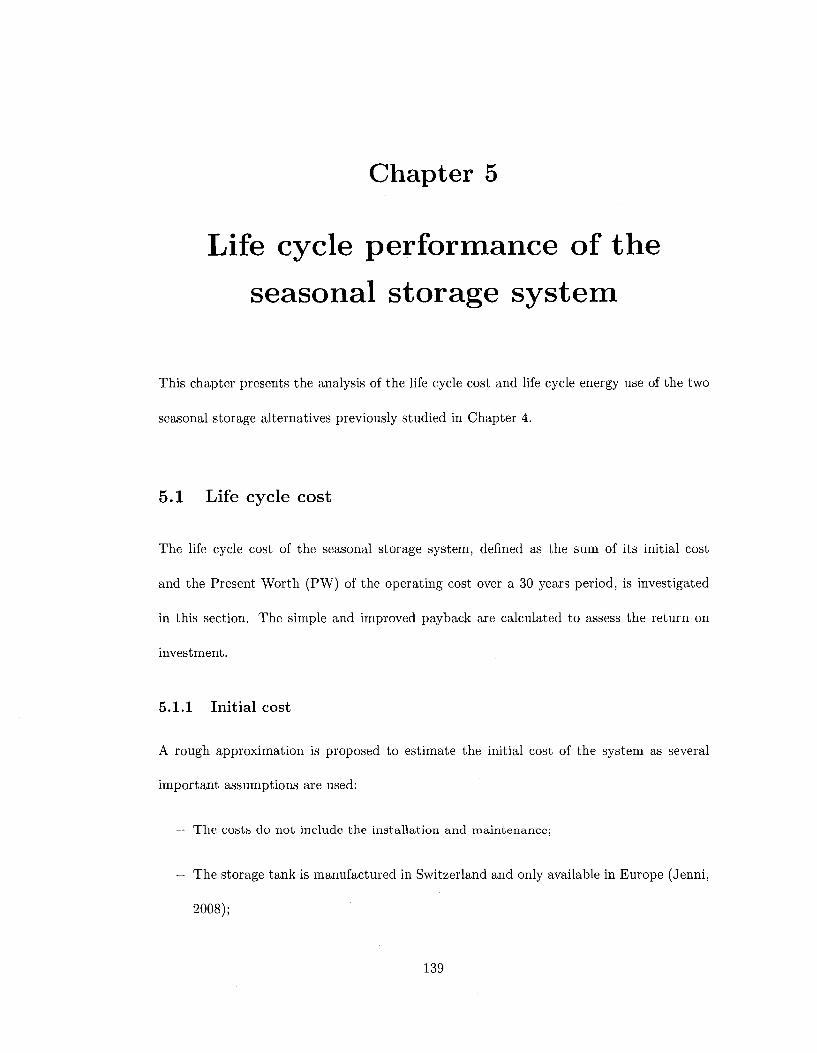
Chapter 5
Life cycle performance of the
seasonal storage system
This chapter presents the analysis of the life cycle cost and life cycle energy use of the two
seasonal storage alternatives previously studied in Chapter 4.
5.1 Life cycle cost
The life cycle cost of the seasonal storage system, defined as the sum of its initial cost
and the Present Worth (PW) of the operating cost over a 30 years period, is investigated
in this section. The simple and improved payback are calculated to assess the return on
investment.
5.1.1 Initial cost
A rough approximation is proposed to estimate the initial cost of the system as several
important assumptions are used:
— The costs do not include the installation and maintenance;
— The storage tank is manufactured in Switzerland and only available in Europe (Jenni,
2008);
139

- The costs of the two external heat exchangers are not considered since no information
has been found;
— The costs of the control units are assumed based on the solar tank manufacturer's
documentation.
Since the combisytem provides space heating and domestic hot water, the electric baseboard
heaters and the conventional electric water heater are not necessary. Therefore, both
alternatives are credited with the initial costs of these systems. However, the additional
cost of cross-linked polyethylene pipes (PEX) integrated in the radiant heating floor needs
to be considered. Also, the flat-plate collectors are supposed integrated to the roof, which
implies the substitution of an equivalent surface of asphalt shingles.
The initial cost is estimated at 58,162 $ for alternative 1 and 39,949 $ for alternative 2
(Table 5.1). The main cost difference comes from the collectors where evacuated tube
(35,603 $) represent more than twice the price of flat-plate collectors (17,238 $).
Table 5.1. Initial cost of the solar combisystem
System component
Storage tank
Tank insulation
Conventional storage tank
Electric baseboard heaters
Radiant floor (PEX pipes)
Solar collectors
Shingles (credit for integrated mounting)
Control unit
Pumps Stratos ECO
P u m p Stratos ECO-ST (Solar pump n ° l )
Tankless water heaters
Copper pipes
Piping insulation
Total
Alternative 1
[$] 12,031
4,777
-1,053
-3,097
2,502
35,603
-2,280
1,328
474
1,331
1,784
202
58,162
Alternative 2
[$] 13,023
5,138
-1,053
-3,097
2,502
17,238
-1,201
2,280
1,328
474
1,331
1,784
202
39,949
Source of da ta
Jenni (2008)
Jenni (2008)
RSMeans (2007)
RSMeans (2007)
RSMeans (2007)
Viessmann (2008)
RSMeans (2007)
Jenni (2008)
Wilo (2008)
Wilo (2008)
Eemax (2008)
RSMeans (2007)
RSMeans (2007)
140

5.1.2 Operating cost
Based on the total electricity use of the solar combisystem QComU (Table 4.41) and using
the electricity rates of Hydro-Quebec (2008), the annual operating costs are estimated at
26 $ for the alternative 1 and 40 $ for the alternative 2.
The inflation rate of electricity is assumed at 2% and the effective interest rate at 3.22% ,
which corresponds to default economic conditions used in Chapter 3. The degradation of
performance is not considered. Based on Equations 3.6 and 3.8, the PW and the life cycle
cost are then equal to 637 $ and 58,799 $ for the design alternative 1; 990$ and 40,939 $
for the alternative 2.
5.1.3 Simple payback
The simple payback of the solar combisystem is calculated as:
Payback = ——J , (5.1) boiar Savings
where:
Payback = simple payback [years];
Ci — initial cost [$]; and
Solar Savings = savings for space and water heating, due to the proposed design
alternative during the first year of operation [$].
As shown in Table 5.3, the simple payback is 79.4 years for alternative 1 and 55.6 years for
alternative 2.
141

Table 5.3. Simple payback of the design alternatives
Alternative
"Best case"
1
2
Electricity i
[kWh]
10,704
365
567
use Operating
[$] 759
26
40
cost Solar Savings
[$] -
733
719
Simple payback
[years]
-
79.4
55.6
1 Based on Hydro-Quebec electricity rates (see Chapter 3).
5.1.4 Improved payback
Compared to the simple payback, the improved payback is a much more realistic approach
as it considers the time value of money. Defined as the period required for the cumulative
savings to equal the initial cost of the system, it is found by solving the following equation
for N (ASHRAE, 2007);
_ Solar Savings (1 + JE)N~1 ,. „x d - ( 1 _ .l)N (5.2)
where:
Ci = initial cost of the design alternative [$];
Solar Savings = savings due to the proposed design alternative during the first
year of operation [$];
JE — inflation rate of electricity [-];
i' = effective interest rate [-]; and
N = number of years [-].
The inflation rate of electricity is assumed at 2% and the effective interest rate at 3.22%.
Based on these assumptions, the cumulative savings are calculated from Equation 5.2.
142
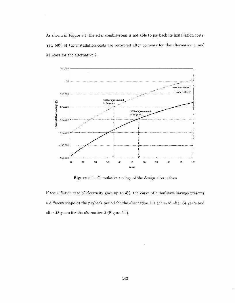
As shown in Figure 5.1, the solar combisystem is not able to payback its installation costs.
Yet, 50% of the installation costs are recovered after 55 years for the alternative 1, and
34 years for the alternative 2.
$10,000
So
-$10,000
c -$20,000 '5
•§ -$30,000
-$40,000
-$50,000
-$60,000
.. ^ i i l ,**
- ^ -
50% of C, recovered in 34 years
1 -X**''^
^ r ^
,,
50% of Cj recovered ^
in 55 years _^^^"^
— - -j—-
, V ,
^:--'^^ ——Alternative 1
™w Alternative 2
- —
0 10 20 30 40 50 60 70 80 90 100
Years
Figure 5.1. Cumulative savings of the design alternatives
If the inflation rate of electricity goes up to 4%, the curve of cumulative savings presents
a different shape as the payback period for the alternative 1 is achieved after 64 years and
after 48 years for the alternative 2 (Figure 5.2).
143

$80,000
$60,000
$40,000
e" $20,000
$0
-$20,000
-$40,000
-$60,000
-Alternative 1
-Alternative 2
Payback = 48 years
Figure 5.2. Impact of the inflation rate of electricity on cumulative savings
Through its ecoEnergy Retrofit program, Natural Resources Canada provides financial
support to homeowners to help them implement energy saving projects that reduce energy-
related greenhouse gases and air pollution (NRCan, 2008). It offers a 500 $ grant for the
installation of a solar domestic hot water system.
Recently, the inflation rate j has surged and is now measured at 3.5% in Canada (Statistics
Canada, 2008). So, by considering the ecoEnergy rebate, the current discount rate i of
4.75% (August 2008) and assuming the inflation of electricity JE equals to the inflation, the
system is now able to recover its installation costs over a 45 years period for the alternative 1,
and over 36 years for alternative 2 (Figure 5.3).
As illustrated previously, a grant of 500 $ is not sufficient to reduce significantly the payback
period of the seasonal storage system. Much more "generous" programs than ecoEnergy
144

$20,000 •
$20,000 •
$40,000 -
^, , - '""""
Payback = 36 years
» , . - " • " " " '
* f » ^ ' ~~jr~ s
^S"^ i
^ f ^ " ^ *
|
J.
y /
-"-Al ternat ive 1 /
• ™ Alternative 2 ./
• ._/- j/r
,' S
. Payback = 45 years
1
30
Years
Figure 5.3. Impact of recent economical data and ecoEnergy program on cumulative savings
exist in other part of the world. For instance, in Belgium, the federal government covers
up to 40% of the investment costs (with a maximum of 5,200 $) as tax rebates for the
installation of a solar thermal system (SPF Economy, 2008). The Walloon Region adds a
grant of 2,280 $ for systems with a net aperture area of collectors ranging between 2 and
4 m2, and 150 $ per additional m2 (Walloon Region Ministry, 2008). Also, residents of the
Wallonia's capital (Namur) benefit from an additional 380 $ from the city authorities (City
of Namur, 2008). So, if such a program would exist in Canada, the total of grants would
be 12,748 $ for alternative 1 and 14,679 S for alternative 2. Using the same rates as the
previous scenario, this would imply a payback time period of 38 years for alternatives 1 and
26 years for alternative 2.
145

$60,000
$40,000
$20,000
$0
-$20,000
-$40,000
-$60,000
30
Years
——Alternative 1 ^ /
^^Alternative 2 yr f
7/ Payback = 26 years ^ " ^r
> * l Payback - 38 years
^ ^ ^ \
40
Figure 5.4. Impact of incentives on cumulative savings
5.1.5 Discussion
The (improved) payback period of the seasonal storage system is quite long as, depending
on the economic scenario, it ranges from 55 to 38 years for the alternative 1, and from 34 to
26 years for the alternative 2 (Table 5.5). The only way to obtain a payback period lower
than the 30-years life span of the system, is to benefit from substantial incentives. These
results are seen as the direct consequence of the high initial costs of the systems in addition
to the low rates of electricity in Quebec, compared to other Canadian provinces (BC Hydro,
2003).
146

Table 5.5. Improved payback for different economic situations
i
[%] 5.54
5.54
4.75
4.75
3
[%] 2.24
2.24
3.50
3.50
»'
[%] 3.22
3.22
1.21
1.21
3E
[%] 2.00
4.00
3.50
3.50
Grant
[$] --
500
12,748
Alternative 1
Payback50%
[years]
55
36
28
18
Payback
[years]
-64
45
38
Grant
[$] --
500
14,679
Alternative 2
Payback50%
[years]
34
26
21
7
Payback
[years]
-48
36
26
5.2 Life cycle energy use
The life cycle energy use relates to the total energy input over the entire life span of the
solar combisystem. Within the scope of this study, the embodied energy of the system's
components and the total operating energy use are evaluated. The estimation does not
take into account the energy required for the unit packing, transportation, installation and
maintenance.
5.2.1 Embodied energy
The estimation of the embodied energy of the two design alternatives is based on some
important assumptions:
- The embodied energy of the storage tank, pumps, piping and external heat exchangers
is limited to an approximation of the embodied energy of materials;
— The tankless water heaters providing auxiliary energy for space heating and hot water
are not considered.
The embodied energy of the evacuated tube collectors is based on one study due to the lack of
detailed information available in the literature. Therefore, the embodied energy is assumed
at 1,521 MJ/m2, and 71,717 MJ for the total collector area of 47.1 m2(Gurzenich and
Mathur, 1998). The assessment of the total embodied (primary) energy required to produce
147

a complete flat-plate collector is based on several studies (Table 5.6). T h e resul ts show some
dissimilarit ies since (i) the mater ia ls used in the solar collectors are not all identical, and (ii)
t he au thors are coming from dist inct countries implying different calculat ion of the p r imary
energy. Consider ing these limits, t h e average value of 1,732 M J / m 2 is t h e n considered. For
t h e to t a l collector area (53 m 2 ) , the embodied energy is calculated at 91,766 M J .
T a b l e 5 .6 . Embodied energy of flat-plate solar collectors
Ac
[m2]
2.13
1.35
5.00
5.00
6.15
5.76
2.00
Embodied
[MJ]
3,513
2,663
6,408
8,633
11,450
9,790
3,604
Average
energy
[MJ/m2]
1,649
1,973
1,282
1,727
1,862
1,700
1,802
1,732
Country
Italy
Cyprus Germany
Germany
Germany
Germany
India
Authors
Ardente et al. (2005)
Kalogirou (2008)
Streicher et al. (2004)
Streicher et al. (2004)
Giirzenich and Mathur (1998)
Giirzenich and Mathur (1998)
Giirzenich and Mathur (1998)
The calculation of the total embodied energy is shown in Table 5.7. The storage tank is
supposed entirely made of stainless steel (16.3 MJ/kg) and recovered by 20 cm of mineral
wool (15.6 MJ/kg). Copper pipes (48.7 MJ/kg) between the collectors and the storage tank
have a diameter of 31.8 mm and are insulated with fiberglass (30.3 MJ/kg) over a total
length of 20 m. The heat exchangers are made of stainless steel (16.3 MJ/kg) (GEA, 2008);
the pumps of stainless steel and grey cast iron (32.8 MJ/kg) (Wilo, 2008).
The electric baseboard heaters previously used to heat the "best case" house are assumed
exclusively made of aluminium (58.5 MJ/kg). They are deducted from the total as well
as the conventional electric water heater (6,155 MJ) (Streicher et al., 2004) and the roof
shingles (76.6 MJ/m 2 ) . The additional embodied energy due the PEX pipes (103.0 MJ/kg)
integrated in the radiant floor is considered.
148

Table 5.7. Total embodied energy of the design alternatives
Element
Collectors
Shingles (credit for roof integration)
Storage tank (stainless steel)2
Insulation (20 cm, mineral wool)
Piping (copper)
Piping insulation (fiberglass)
Antifreeze
Solar heat exchanger
DHW heat exchanger
Pumps
Electric baseboard heaters
Conventional storage tank
[m2]
53.0
53.0
[kg] 3,744.2
260.2
30.9
2.8
55.0
14.0 7.2
12.0
69.5
-
Flat-plate
[MJ/m2]
1,732
76.6
[MJ/kg]1
16.3
15.6
48.7
30.3
42
16.3
16.3
24.6
58.5
-
Total
[MJ]
91,766
-4,058
[MJ]
62,918
4,064
1,504
85
2,311
228
117
295
-4,058
-5,659
157,870
Evacuated tube
[m2]
47.1
-
[kg] 3,369.8
260.2
30.9
2.8
35.1
14.0
7.2
12.0
69.5
-
[MJ/m2]
1,521
-
[MJ/kg]1
16.3
15.6
48.7
30.3 42
16.3
16.3
24.6
58.5
-
Total
[MJ]
71,717
-
[MJ]
54,927
4,064
1,504
85
1,476
228
117
295
-4,058
-5,659
134,689
1 From Yang (2005). 2 The total weight of the storage tank is given by Jenni (2008).
The total embodied energy of the solar combisystem is approximated at 157,870 MJ for the
alternative 1 and 134,689 MJ for the alternative 2.
5.2.2 Operating energy use
To assess the operating energy (primary), the annual electricity use of both combisystems
Qcombi (Table 4.41) is divided by the overall power plant efficiency r)w of 73.1% (see
Chapter 3). Assuming that the annual energy use remains constant over the 30-years
life span of the system, regardless of the efficiency decrease of the mechanical systems or
equipments, the total operating energy use is thus equal to 30 times the annual operating
energy use, and its value is calculated at 53.9 GJ for the alternative 1 and 83.8 GJ for the
alternative 2.
The life cycle energy use of the seasonal storage system is the sum of its embodied energy
149

(Table 5.7) and the operating energy use over 30 years, which gives 188.6 GJ and 241.6 GJ.
5.2.3 Energy payback t ime
The energy payback time (EPT) is defined as the time (in years) in which the amount
of primary energy required to manufacture the solar combisystem is compensated by the
energy produced (Richards and Watt, 2007):
E P T = E^Put ( 5 > 3 )
" n e t , primary
where:
EPT = energy payback time [years];
Einput — embodied energy of the system [GJ]; and
WnettPrimary — annual net energy output in primary energy equivalent [GJ/yr]
The value of Wnettprimary is calculated as:
Wnet,primary — W - ^ / Vpp
With energy payback time values of 4.9 years for the alternative 1 and 6.0 years for the
alternative 2 (Table 5.9), the results are higher than the typical energy payback times of solar
combisystems (without long-term storage capacity) ranging from 2.0 to 4.3 years (Streicher
et al., 2004). Yet, such difference is easily explained by the higher overall efficiency of power
plants in Quebec (73.1%) compared to Germany (35.0%).
150
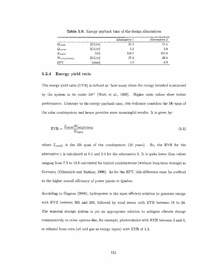
Table 5.9. Energy payback time of the design alternatives
Alternative 1 Alternative 2 [GJ/yr] 2L4 21.4 [GJ/yr] 1.3 2.0
[GJ] 134.7 157.9 [GJ/yr] 27.4 26.4 [years] 4J) ^0_
5.2.4 Energy yield ratio
The energy yield ratio (EYR) is defined as "how many times the energy invested is returned
by the system in its entire life" (Watt et al., 1998). Higher ratio values show better
performance. Contrary to the energy payback time, this indicator considers the life span of
the solar combisystem and hence provides more meaningful results. It is given by:
p v p J-'combi " net {primary (x,<\
^input
where Lcamu is the life span of the combisystem (30 years). So, the EYR for the
alternative 1 is calculated at 6.1 and 5.0 for the alternative 2. It is quite lower than values
ranging from 7.5 to 12.6 calculated for typical combisystems (without long-term storage) in
Germany (Gurzenich and Mathur, 1998). As for the EPT, this difference must be credited
to the higher overall efficiency of power plants in Quebec.
According to Gagnon (2008), hydropower is the most efficient solution to generate energy
with EYR between 205 and 280, followed by wind power with EYR between 18 to 34.
The seasonal storage system is yet an appropriate solution to mitigate climate change
comparatively to other options like, for example, photovoltaics with EYR between 3 and 6,
or ethanol from corn (oil and gas as energy input) with EYR of 1.3.
W loads
combi
et .primary
EPT
Q
151

5.2.5 D i s c u s s i o n
The life cycle cost analysis shows that the proposed design alternatives do not provide
rational payback periods by considering default economic conditions. However, with higher
rates of inflation and with some incentives, the initial costs can be recovered after a more
reasonable period of time.
The great potential of energy savings of the solar combisystem is very well demonstrated on
a life cycle basis. Indeed, the energy payback time and energy yield ratio for both systems
present acceptable values for such a large system. Comparatively to the second alternative
using flat-plate collectors, the first performs better in terms of energy payback time and
energy yield ratio. Due to the higher efficiency of evacuated tube in cold climates, it requires
less collector area and less storage tank volume. Therefore, less material - meaning a lower
embodied energy - is required to achieve approximately the same level of performance
(Wnet
152

Chapter 6
Conclusions, contributions and
future work
6.1 Conclusions
This research has presented the development of the integrated building model of a typical
single family house in Montreal by using the TRNSYS 16 simulation program. Several
design alternatives have been proposed to improve the life cycle performance of the building,
including the life cycle energy, environmental impacts and life cycle cost.
The modelling of a solar thermal application for space and water heating with a long-term
storage capacity is carried out. The overall performance of the system is investigated and
enhanced by performing a sensitivity analysis on a certain set of design parameters. The life
cycle analysis is performed to assess the potential of cost and energy savings of the system
during its entire life span.
The results of the present study lead to the following conclusions:
— The life cycle performance of a single family house can be significantly enhanced by
combining a passive solar design, high level of thermal insulation, high performance
windows and airtightness of the building envelope;
— The life cycle energy and emission of the house are reduced by choosing materials
153

with low embodied energy;
— The solar combisystem with seasonal storage capacity is a concept that is achievable
in a cold climate like Canada;
— The system performs better with evacuated tube collectors, compared to flat-plate
collectors;
— The sensitivity analysis shows the essential role of the storage tank insulation on the
sizing and the overall performance of the system;
— Key design features such as the tilt angle and the mass flow rate circulating in the
solar loop have to be considered carefully;
— The life cycle energy analysis shows that the systems provide substantial energy
savings.
More globally, the study reveals that the life cycle cost analysis of both the house and the
solar combisystem are directly "affected" by the low electricity rates in Quebec. Indeed, the
results would be totally different in other Canadian provinces and the proposed solutions
would lower the payback periods drastically. In addition, since 95% of electricity in Quebec
is generated by cleaner alternatives like hydropower (see Chapter 3), the life cycle energy
use of the house and system is reduced. Though this can be perceived as an excellent news,
this has the negative effect to lower the energy payback and market penetration of such
"green alternatives".
6.2 Research contributions
This study has brought the following contributions:
154

— Review of existing and future projects of low energy and net-zero houses in different
parts of the world;
— Identification of key design features for low energy buildings and solar combisystems;
— Modelling of an advanced solar combisystem with a long-term thermal storage capacity
in a cold climate;
— One-dimension sensitivity analysis of the solar combisystem based on a certain set of
design parameters;
— Investigation of the life cycle energy use and life cycle cost of the solar combisystem.
6.3 Recommendations for future work
Several research directions using this thesis as a starting point can be identified.
Solar combisystem
Although many design parameters of the solar combisystem are evaluated in this research,
other aspects are expected to have a considerable impact:
— PV (photovoltaic) cells can be used to power the Solar pump n°l and provide a con
tinual adjustment of fluid flow, and possibly improving the system performance (Al-
Ibrahirn, 1997). Indeed, this system can act as a fast-response sensor to solar energy
and therefore pumping will only occur at the times when the thermal collector is also
receiving solar radiation. Also, the use of a PV power source eliminates the demand
for an auxiliary power source to operate the pump;
155

— The degree of precision to model the storage tank can be enhanced by increasing the
number of layers;
— The flow rate of the Solar pump n°2 can be fixed to limit the flow in the stratifying
device to the recommended range of 5-8 kg/min (see Chapter 2);
— To avoid exploiting the hottest water in the tank (located in the top layer), different
outlet locations can be investigated since the maximum water temperature for space
heating is only 45° C;
— Since the storage tank is expected to store water at high temperatures during summer
months, a sensitivity analysis on the thickness of insulation can be achieved to see the
effect on the cooling loads of the house;
— To reduce the electricity use of the ventilation system, the hot water contained in the
tank can be used to preheat the cold outdoor air in winter thanks to a heat exchanger.
Finally, this research can be extent to other locations in Canada to quantify the effect of
different climatic conditions on the system's design. The life cycle performance, including
the life cycle cost and energy savings, would be significantly affected as well due to higher
utility rates and other source of electricity generation.
156

References
Aguilar, C , White, D., and Ryan, D. (2005). Domestic Water Heating and Water Heater
Energy Consumption in Canada. CBEEDAC, Canadian Building Energy End-Use Data
and Analysis Centre. University of Alberta, Edmonton, AB,
Aitken, D. (2003). Transitioning to a renewable energy future. In ISES International solar
energy society white paper, Freiburg.
Al-Ibrahim, A. (1997). Optimum Selection of Direct-Coupled Photovoltaic Pumping System
in Solar Domestic Hot Water Systems. PhD thesis, University of Wisconsin-Madison.
Andersen, E., Furbo, S., Hampel, M., Heidemann, W., and Muller-Steinhagen, H. (2008).
Investigation on stratification devices for hot water heat stores. International Journal of
Energy Research, 32:255-263.
Ardente, F., Beccali, G., Cellura, M., and Lo Brano, V. (2005). Life cycle assessment of a
solar thermal collector. Renewable Energy, 30:1031-1054.
ASHRAE (2001). ASHRAE Standard 62-2001. Ventilation for acceptable indoor air
quality. American Society of Heating, Refrigerating and Air-Conditioning Engineers,
Inc., Atlanta.
ASHRAE (2004). ASHRAE Standard 55-2004. Thermal environmental conditions for
human occupancy. American Society of Heating, Refrigerating and Air-Conditioning
Engineers, Inc., Atlanta.
157

ASHRAE (2005). ASHRAE Handbook-Fundamentals. American Society of Heating,
Refrigerating and Air-Conditioning Engineers, Inc., Atlanta.
ASHRAE (2007). ASHRAE Handbook-HVAC Applications. American Society of Heating,
Refrigerating and Air-Conditioning Engineers, Inc., Atlanta.
ASHRAE Montreal Chapter (2007). Website, http://www.ashrae-mtl.org/ (Last accessed
March 6, 2007).
ATHENA (2003). Environmental impact estimator v 3.0. Athena Sustainable Materials
Institute. Ottawa, Canada.
Athienitis, A. K. and Santamouris, M. (2002). Thermal Analysis and Design of Passive
Solar Buildngs. James & James.
Bales, C. and Persson, T. (2003). E xternal DHW units for solar combisystems. Solar
Energy, 74:193-204.
Baouendi, R. (2003). Development of a prototype tool for the evaluation of sustainability
of Canadian houses. Master's thesis, Concordia University, Montreal, Canada.
BC Hydro (2003). Electric Rates Comparison. Technical report, BC Hydro.
http://www.bchydro.com/rxJiles/info/info9238.pdf (Last accessed December 13, 2007).
Beasley, D. and Clark, J. (1984). Transient response of a packed for thermal energy storage
bed. International Journal of Heat and Mass Transfer, 27:1659-1669.
BedZED & Eco-Village Development (2007). Website, http://www.bioregional.com (Last
accessed March 5, 2007).
158
Braun, J., Klein, S., and Mitchell, J. (1981). Seasonal storage of energy in solar heating.
Solar Energy, 26:403-411.
CEPHEUS (2001). Final Technical Report, http://www.passivehouse.com (Last accessed
March 7, 2007).
Charron, R. (2005). A review of low and net-zero energy solar homes initiatives.
Technical report, CANMET Energy Technology Centre-Varennes, NRCan. http://cetc-
varennes.nrcan.gc.ca (Last accessed March 5, 2007).
City of Namur (2008). Website. http://www.energie-namur.be/ (Last accessed
September 26, 2008).
Cruickshank, C. A. and Harrison, S. J. (2006). Simulation and testing of stratified multi-
tank, thermal storages for solar heating systems. In EuroSun 2006, Glasgow, UK.
Dayan, M. (1997). High performance in low-flow solar domestic hot water systems. Master's
thesis, University of Wisconsin-Madison.
Dincer, I., Dost, S., and Li, X. (1997). Performance analyses of sensible heat storage systems
for thermal applications. International Journal of Energy Research, 21:1157-1171.
DOE (2008). Website. U.S. Department of Energy.http://www.eere.energy.gov/ (Last
accessed October 5, 2008).
Duffle, J. and Beckman, W. (2006). Solar Engineering of Thermal Processes. John Wiley
& Sons Inc. 3rd Ed.
Eemax (2008). Website, http://www.tanklesswaterheaters.ca/ (Last accessed September 14,
2008).
159

Ellehauge, K. (2003). Final report: Solar Combisystems. Technical report, Altener.
http://www.elle-kilde.dk/altener-comb (Last accessed October 5, 2008).
EnergyPlus (2007). EnergyPlus Engineering Reference. US Department Of Energy.
Environment Canada (2007). Canadian Climate Normals 1971-2000.
http://www.climate.weatheroffice.ec.gc.ca (Last accessed July 9, 2007).
EQuilibrium Housing (2007). Website, http://www.cmhc-schl.gc.ca (Last accessed March 5,
2007).
Frei, U., Vogelsanger, P., and Homberger, D. (2000). Domestic hot water systems: testing,
development, trends. In 3rd ISES-Europe Solar Congress, EuroSun 2000, Copenhagen.
Fujitsu (2007). Website, http://www.fujitsugeneral.com/ (Last accessed December 5, 2007).
Gagnon, L. (2008). Civilisation and energy payback. Energy Policy, 39:3317-3322.
Gagnon, L., Belanger, C , and Uchiyama, Y. (2002). Life-cycle assessment of electricity
generation options: The status of research in year 2001. Energy Policy, 30:1267-1278.
Garg, H. P., Mullick, S. C , and Bhargava, A. K. (1985). Solar Thermal Energy Storage.
Springer.
GEA (2008). Website, http://www.flatplate.com/ (Last accessed October 2, 2008).
Gerbasi, D. (2000). The Energy Performance of the NOVTEC Advanced House. Master's
thesis, Concordia University.
Gurzenich, D. and Mathur, J. (1998). Material and energy demand for selected renewable
energy technologies. Technical report, DLR - International Bureau of the BMBF.
Hadorn, J.-C. (2005). Thermal energy storage for solar and low energy buildings. IEA SHC.
160

Haines, G., Org, M., Barkan, A., and Pressnail, K. (2007). An economic and environmental
comparison of standard versus energy efficient homes in toronto, Canada. In Sustainable
Urban Areas, Rotterdam, Netherlands.
Hamada, Y., Nakamura, M., Ochifuji, K., Yokoyama, S., and Nagano, K. (2003).
Development of a database of low energy homes around the world and analyses of their
trends. Renewable Energy, 28(2):321-328.
Hasnain, S. (1998). Review on sustainable thermal energy storage technologies, part 1: Heat
storage materials and techniques. Energy Conversion and Management, 39:1127-1138.
Heimrath, R. (2003). Generic System #19: Centralized Heat Production, Distributed Heat
Load. Technical report, IEA SHC - Task 26. http://www.iea-shc.org/outputs/task26/
(Last accessed March 28, 2008).
Hestnes, A. G., Hastings, R., and Saxhof, B. (2003). Solar energy houses: strategies,
technologies, examples. James & James, 2nd edition.
Hunn, B. and Calafell, D. (1977). Determination of average ground reflectivity for solar
collectors. Solar Energy, 19:87-89.
Hydro-Quebec (2008). Website. http://www.hydroquebec.com/ (Last accessed
September 22, 2008).
IEA SHC (2007). International Energy Agency. Solar Heating and Cooling. Website.
http://www.iea-shc.org (Last accessed March 8, 2007).
IPCC (2007). Intergovernmental panel on climate change, website, http://www.ipcc.ch/
(Last accessed November 2, 2007).
Jenni (2008). Website, http://www.jenni.ch/ (Last accessed September 21, 2008).
161

Jordan, U. and Vajen, K. (2001). Realistic domestic hot-water profiles in different time
scales. Technical Report V. 2.0, FB. Physik, FG. Solar. Universitat Marburg.
Kalogirou, S. (2008). Thermal performance, economic and environmental life cycle analysis
of thermosiphon solar water heaters. Solar Energy. doi:10.1016/j.solener.2008.06.005.
Kassab, M. (2002). Improving the energy performance of houses in montreal using the
life-cycle analysis. Master's thesis, Concordia University, Montreal, Canada.
Kasuda, T. and Archenbach, P. (1965). Earth temperature and thermal diffusivity at
selected stations in the United States. ASHRAE Transactions, 71:61-74.
Keller, B. (1998). Low temperature heating and cooling systems for low-energy houses.
Proved in practice, In Proceedings of the IEA workshop "Future building forum - Low
temperature heating systems in buildings", Royal Institue of Technology, Stockholm,
Sweden.
Kenjo, L., Caccavelli, D., and Inard, C. (2003). A model of low flow solar domestic hot
water system. In 8th International IBPSA Conference, Eindhoven, Netherlands.
Kjarstad, J. and Johnsson, F. (2007). The european power plant infrastructure -
Presentation of the Chalmers energy infrastructure database with applications. Energy
Policy, 35:3643-3664.
Krause, T. and Jaehnig, D. (2002). Solar heating with a storage-integrated condensing gas
burner. In Indudstry Workshop, IEA-SHC Task 26.
Liu, W., Davidson, J., and Mantell, S. (2000). Thermal analysis of polymer heat exchangers
for solar water heating: A case study. Journal of Solar Energy Engineering, 122(2):84-91.
162

Lstiburek, J. (2002). Relative humidity. In Proceedings of the Healthy Indoor Environments
Conference, April 23, 2002, Austin, Texas.
M. CONDE Engineering (2002). Thermophysical Properties of Brines. Technical
report. http://www.mrc-eng.com/Downloads/Brine%20Properties.pdf (Last accessed
February 1, 2008).
MNECCH (1997). Model National Energy Code of Canada for Houses. NRC, National
Research Council of Canada. Canadian Commission on Buildings and Fire Codes. Ottawa,
Canada.
Morrison, G., Budihardjo, I., and Behnia, M. (2005). Measurement and simulation of flow
rate in a water-in-glass evacuated tube solar water heater. Solar Energy, 78:257-267.
Nallusamy, N., Sampath, S., and Velraj, R. (2007). Experimental investigation on a
combined sensible and latent heat storage system integrated with constant/varying (solar)
heat sources. Renewable Energy, 32:1206-1227.
Net-Zero Energy Home Coalition (2007). Website, http://www.netzeroenergyhome.ca/
(Last accessed March 8, 2007).
NRCan (2005). R-2000 Standard. Office of Energy Efficiency, http://oee.nrcan.gc.ca (Last
accessed March 23, 2007).
NRCan (2006). Energy Use Data Handbook, 1990 and 1998 to 2001 Office of Energy
Efficiency. http://oee.nrcan.gc.ca/Publications/statistics/handbook06 (Last accessed
March 2, 2007).
NRCan (2008). Website, http://www.nrcan.gc.ca/ (Last accessed September 15, 2008).
163

Passive Houses in Europe, CEPHEUS (2007). Website, http://www.cepheus.de/ (Last
accessed March 5, 2007).
Pierce, M. (2000). Energy saving window treatments. Cornell Cooperative Extension.
Department of Design & Environmental Analysis, Cornell University.
Province of Quebec (1992). Regulation respecting energy conservation in new buildings.
Publications du Quebec, Quebec.
RETScreen (2007). NRCan. website, http://www.retscreen.net/ (Last accessed June 29,
2007).
Richards, B. and Watt, M. (2007). Permanently dispelling a myth of photovoltaics via
the adoption of a new net energy indicator. Renewable and Sustainable Energy Reviews,
11:162-172.
RSMeans (2007). RSMeans Residential Cost Data 2007, volume 26. RSMeans Comp.,
Kingston, MA.
Schnieders, J. and Hermelink, A. (2006). CEPHEUS results: measurements and occupants'
satisfaction provide evidence for Passive Houses being an option for sustainable building.
Energy Policy, 34(2):151-171.
SEL (2007). TRNSYS 16. A Transient Simulation Program. University of Wisconsin,
Madison, WI.
Shah, L,, Andersen, E., and Furbo, S. (2005). Theoretical and experimental investigations
of inlet stratifiers for solar storage tanks. Applied Thermal Engineering, 25:2086-2099.
Smeds, J. and Wall, M. (2007). Enhanced energy conservation in houses through high
performance design. Energy and Buildings, 39(3):273-278.
164

Solar Building Research Network (SBRN) (2007). Website, http://www.solarbuildings.ca
(Last accessed March 5, 2007).
Solvis (2007). Website, http://www.solvis.de/ (Last accessed May 23, 2007).
SPF Economy (2008). Website, http://mineco.fgov.be/energy/ (Last accessed March 5,
2007).
SRCC (2008). Directory of SRCC certified solar collector ratings. Technical report,
Solar Rating and Certification Corporation, http://www.solar-rating.org/ (Last accessed
February 1, 2008).
Statistics Canada (2005). Electric power generation, transmission and distribution.
Catalogue no. 57-202-XIE.
Statistics Canada (2008). Website, http://www.statscan.ca/ (Last accessed September 22,
2008).
Streicher, E., Heidemann, W., and Muller-Steinhagen, H. (2004). Energy payback time - A
key number for the assessment of thermal solar systems. In Proceedings of Eurosun 2004,
20-23 June 2004, Freiburg, Germany.
Technischen Universitat Berlin (2007). Website, http://www.tu-berlin.de/ (Last accessed
April 5, 2007).
Tepe, R., Bales, C , Bony, J., Pittet, T., and Heimrath, R. (2004). Elements and examples
of "Dream Systems" of solar combisystems. Technical report, IEA SHC - Task 26.
TESS (2007). TESS Library Documentation. Thermal Energy System Specialists, Madison,
WI.
165
The Building Group, NRCan (2007). Website, http://www.buildingsgroup.nrcan.gc.ca
(Last accessed March 6, 2007).
Thevenard, D. and Haddad, K. (2006). Ground reflectivity in the context of building energy
simulation. Energy and Buildings, 38:972-980.
Thomsen, K. E., Schultz, J. M., and Poel, B. (2005). Measured performance of 12
demonstration projects - IEA Task 13 "Advanced solar low energy buildings". Energy
and Buildings, 37(2):111-119.
Thiir, A. (2007). Compact Solar Combisystem. PhD thesis, Danmarks Tekniske Universitet.
UNFCCC (2008). Website. United Nations Framework Convetion on Climate Change.
http://unfccc.int/ (Last accessed March 2, 2008).
UNIPHIZ Lab (2007). Findgraph v 1.860. http://www.uniphiz.com/ (Last accessed July 26,
2007).
Van der Veken, J., Peeters, L., and Hens, H. (2005). Comparison of heating
system in a residential building. In Building Simulation 2005, Ninth International
IBPSA Conference. http://www.ibpsa.org/proceedings/BS2005/BS05.1277_1284.pdf
(Last accessed October 10, 2007).
van Moeseke, G., Bruyere, I., and De Herde, A. (2007). Impact of control rules on
the efficiency of shading devices and free cooling for office buildings. Building and
Environment, 42:784-793.
Venmar (2007). Website, http://www.venmar.ca/ (Last accessed October 11, 2007).
Viessmann (2008). Website, http://www.viessmann.de/ (Last accessed January 31, 2008).
166

Wall, M. (2006). Energy-efficient terrace houses in Sweden: Simulations and measurements.
Energy and Buildings, 38(6):627-634.
Walloon Region Ministry (2008). Website. General Directorate for Technology, Research
and Energy, http://www.cepheus.de/ (Last accessed September 26, 2008).
Watt, M. E., Johnson, A. J., Ellis, M., and Outhred, H. R. (1998). Life-cycle air emissions
from pv power systems. Progress in Photovoltaics: Research and Applications, 6:127-136.
Weiss, W. (2003). Solar Heating Systems for Houses: A design handbook for solar
combisystems. IEA SHC.
Weiss, W., Bergmann, I., and Faninger, G. (2008). Solar Heat Worldwide - Markets and
Contribution to the Energy Supply 2006. Technical report, IEA SHC.
Welfonder, T., Hiller, M., Hoist, S., and Knirsch, A. (2003). Improvements on the
capabilities of trnsys 15. In Eighth International IBPSA Conference, Eindhoven,
Netherlands.
Wiedemann, T. (2004). World in Transition: Towards Sustainable Energy Systems.
Inderscience Publishers.
Wilo (2008). Website, http://www.wilo.com/ (Last accessed March 29, 2008).
Yang, L. (2005). Life cycle analysis of the residential HVAC systems in montreal. Master's
thesis, Concordia University.
Zmeureanu, R., Fazio, P., DePani, S., and Calla, R. (1998a). Development of an energy
rating system for existing houses. Energy and Buildings, 29:107-119.
167

Zmeureanu, R., Marceau, M. L., Payer, J., and Derome, D. (1998b). Evaluation of energy
performance of nine identical row houses in montreal. In Thermal Performance of the
Exterior Envelopes of Buildings VII, Clearwater Beach, Florida.
Zmeureanu, R. and Wu, X. (2007). Energy and exergy performance of residential heating
systems with separate mechanical ventilation. Energy, 32:187-195.
168

Appendices
169

Appendix A
Technical specifications of the HRV system
Dimensions and Service Clearances: VenmarAVS NOVOFIT 1.5 r Hanging Chains/Springs Mounling Localion
Ventilation Performance EXTS PRES Pa 25 50 75 100 125 150 175 200
TATIC SURE hwg.
.1
.2
.3
.4
.5
.6
.7
.8
NE A
l/s 83 79 75 71 64 59 53 43
TSUP RFLO cfm 175 168 159 150 136 126 113 91
>LY
W
m!/h 299 285 270 256 230 214 192 155
l/s " 83 80 75 71 64 60 53 43
CR UPPL* c fm 176 169 159 151 136 127 113 91
OSS A < m'/h 299 288 270 256 230 216 192 155
IRFLC E.
l/s 83 78 75 69 60 48 38 21
)W XHAU
cfm 175 165 158
146 127 103 80 45
>T
m'/h 295 281 270 248 216 173 136 76
is J •
o...
'"•- • « . . .
^*\
1 —-Supply (l/sl
-"Exhausl lift)
0 50 100 150 200 CFM ( l /s - CFM X 0.471 9) ( m ' / h = 1/5 x 3.6)
Energy Performance SUPPLY
TEMPERATURE C ! F"
HEATING 0 0 0
-2 5 -2 5
+ 37 + 32 + 32 -13 -13
COOLINC + 35 h-95 + 35 H-95
NET AIRFLOW l/s cfm
31 56
37
—
66 119
7$
—
m'/h
117 /m 133
—
POWER CONSUMED
WATTS
85 124
114
—
SENSIBLE RECOVERY EFFICIENCY
69 60 62
—
APPARENT SENSIBLE 5FJECWNB5
81 70
80
—
LfflKISCMW MOISTURE TRANSFER
- 0 . 01 -0 .01
0.08
— TOTAL REC0WRY EFFICIENCY
Not tested
— 1
1 (%) 1 — N9!(%) j
NOTE:
I Air Flow - l/s (0 .47 l/s « 1 CFM)
All specifications are subject to change without notice.
Specifications and Ratings • M o d e l : V e n m a r AVS NOVOFIT 1.5
• Part Number : 4 3 1 2 0
• Total Assembled Weight: (Including polypropylene core) 65 lb (29.5 kg)
• Supply and Exhaust Air Duct Connections: 6" (1 5.24 cm) diameter
• Drains: W (1.2 cm) fittings with 10 ft (3 m) PVC drain
• F i l ters : - 1 5 ppi washable reticulated foam
- 1 5.375" X 7.1 25" X 0.75"
(39 X 1 8 x 1 . 9 cm)
• Cabinet: 20 ga. pre-painted steel • Insulation: 1" (2.54 cm) aluminum foil
faced fiberglass 0.825" (2.10 cm) expanded polystyrene
•Mounting: suspension by chains and springs
• Supply & Exhaust Blower Motor : 1 m o t o r
- Protection type: Thermally protected - I nsu la t i on c lass: B
- V (motor marking): 120 V ac, 50/60 Hz, 1.2/1.0 A, 1 050/1 300/1 660 RPM
• Fan Speed Control: -Low, increased low & high speed -Two speeds available to user -Low or increased low speed is
selected at the time of installation • Heat Recovery Core:
- Heat Exchange Surface Area: 102 f t ! (9.54 m2)
-Type/Material: Crossflow/ Polypropylene • Unit Electrical Characteristics:
Volts Freq. Amps Watts IP 120 60 Hz 1.3 150
Submitted by:
Qty: Model No.:
Date: Remarks:
Project.
Location:
Architect:
Engineer:
Contractor:
HVI
J ^ / S Residential Product Croup, 550 Lemire Blvd. Drummondville, QC, Canada J2C7W9-Tel . : 1-800-567-3855 Fax: 1-800-567-1715
05 /07 PRODUCT SHEET no. 91197 A4&.® w w w . v e n m a r . c a
170

Appendix B
Coefficients used to calculate the temperature of cold water from the city line
n harmonic
1
2
3
4
5
6
7
8
9
10
11
12
13
14
15
16
17
Cn
0.18399457
-6.7763674
-0.096571472
0.084368625
-0.0031887082
-0.09697441
0.014070618
-0.33625031
-0.027762869
-0.036247456
-0.013672282
-0.018720731
-0.0066015323
-0.089322769
-0.04498332
0.17270848
0.024281561
dn
0.09056716
-7.3992997
-0.20339461
0.88293357
-0.037057249
0.1161188
-0.022911697
-0.014277327
-0.017975378
-0.13904543
-0.054122503
0.1353561
-0.020641118
0.084332139
-0.012268606
0.068648872
0.00080673597
Coefficient a and b are equal to 11.490452 and 0.0086904361,
respectively.
171
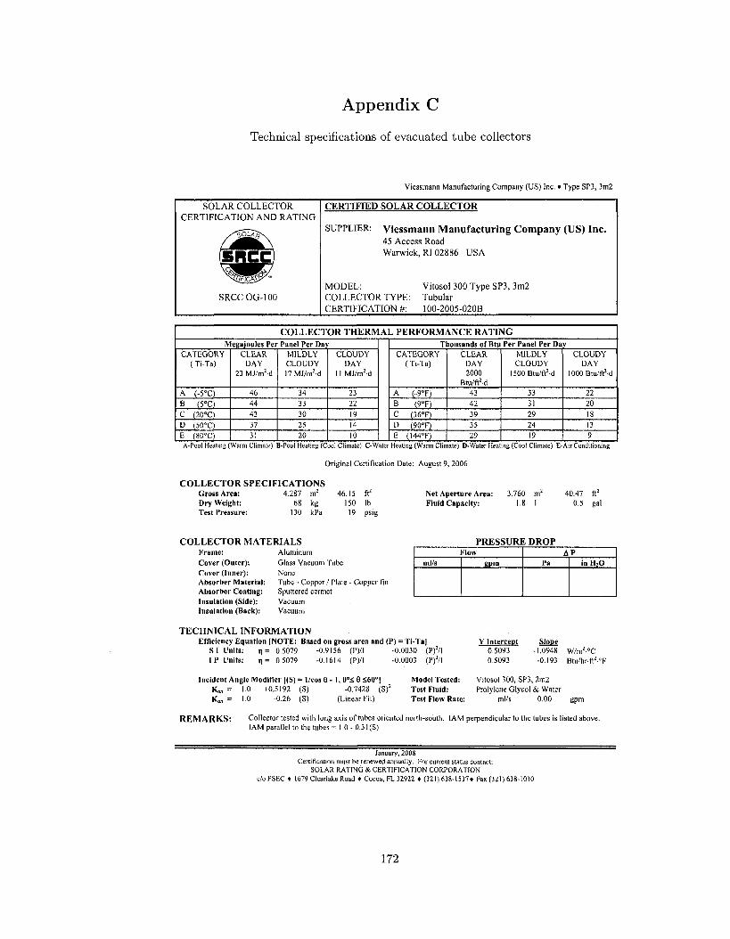
Appendix C
Technical specifications of evacuated tube collectors
Vicssmann Manufacturing Company (US) Inc, • Type SP3, 3m2
SOLAR COLLECTOR CERTIFICATION AND RATING
CERTIFIED SOLAR COLLECTOR
SUPPLIER: Viessmann Manufacturing Company (US) Inc. 45 Access Road
Warwick, RI 02886 USA
MODEL: Vitosol 300 Type SP3, 3m2 COLLECTOR TYPE: Tubular CERTIFICATION*: 100-2005-020B
COLLECTOR THERMAL PERFORMANCE RATING Megajoules Per Panel Per Day
CATEGORY (Ti-Ta)
A (-5°C) B (5°C) C (20°C) D (50°C) E (80°C)
CLEAR DAY
23 MJ/m2d
46 44 42 37 31
MILDLY CLOUDY 17MJ/m2-d
34 33 30 25 20
CLOUDY DAY
11 MJ/m2d
23 22 19 14 10
Thousands of Btu Per Panel Per Day CATEGORY
(Ti-Ta)
A (-9°F) B (9°F) C (36°F) D (90°F) E (144°F)
CLEAR DAY 2000
Btu/ft2d 43 42 39 35 29
MILDLY CLOUDY
1500Btu/ft2d
33 31 29 24 19
CLOUDY DAY
I000Btu/ft2d
22 20 18 13 9
A-Pool Heating (Warm Climate) B-Pool Heating (Cool Climate) C-Water Heating (Warm Climate) D-Water Heating (Cool Climate) E-Air Conditioning
Original Certification Date: August 9, 2006
COLLECTOR SPECIFICATIONS Gross Area: 4.287 m2 46.15 ft2
Dry Weight: 68 kg 150 lb Test Pressure: 130 kPa 19 psig
Net Aperture Area: Fluid Capacity:
3.760 m2
1.8 1 40.47 ft2
0.5 gal
COLLECTOR MATERIALS PRESSURE DROP Frame: Cover (Outer): Cover (Inner): Absorber Material: Absorber Coating: Insulation (Side): Insulation (Back):
Aluminum Glass Vacuum Tube None Tube - Copper / Plate - Copper fin Sputtered cermet Vacuum Vacuum
Flow ml/s Kpm
AP Pa inH 2 0
TECHNICAL INFORMATION Efficiency Equation [NOTE: Based on gross area and (P) = Ti-Ta|
SI Units: T] = 0.5079 -0.9156 (P)/I -0.0030 (P)2/l IP Units: r\= 0.5079 -0.1614 (P)/I -0.0003 (P)2/l
Incident Angle Modifier |(S) - 1/cos 9 - 1 , 0°£ 8 S60°| Model Tested: K„, = 1.0 +0.5192 (S) -0.7428 (S)2 Test Fluid: K«, » 10 -0.26 (S) (Linear Fit) Test Flow Rate:
Y Intercept Slope 0.5093 -1.0948 W7m2°C 0.5093 -0.193 Btu/hr-ft2oF
Vitosol 300, SP3, 2m2 Prolylene Glycol & Water
ml/s 0.00 gpm
REMARKS: Collector tested with long axis of tubes oriented north-south. 1AM perpendicular to the tubes is listed above. IAM parallel to the tubes - 1.0 - 0.31 (S)
January, 2008 Certification must be renewed annually. For current status contact:
SOLAR RATING & CERTIFICATION CORPORATION c/oFSEC • 1679 Clearlake Road • Cocoa, FL 32922 • (321) 638-1537* Fax (321) 638-1010
172

Appendix D
Parameters used in the mathematical models of aqueous solutions of polypropylene glycol
Parameter
Ai
A2
A3
A4
A5
P [kg/m3]
508.41109
-182.40820
965.76507
280.29104
-472,22510
Op
[kj/(kg.°c)]
4.47642
0.60863
-0.71497
-1.93855
0.47873
A
[W/(m-°C)]
1.18886
-1.49110
-0.69682
1.13633
0.06735
M [Pa-s]
-1.02798
-10.03298
-19.93497
14.65802
14.62050
Source: M. CONDE Engineering (2002).
173

Appendix E
Technical specifications of flat-plate collectors
Viessmann Manufacturing Company (US) Inc. • SV1, SHI
SOLAR COLLECTOR CERTIFICATION AND RATING
SRCCOG-100
CERTIFIED SOLAR COLLECTOR
SUPPLIER: Viessmann Manufacturing Company (US) Inc. 45 Access Road Warwick, RI02886 USA
MODEL: Vitosol 100 SV1, SH1 COLLECTOR TYPE: Glazed Flat-Plate CERTIFICATIONS: 100-2005-019A
COLLECTOR THERMAL PERFORMANCE RATING Megajoules Per Panel Per Day
CATEGORY (Ti-Ta)
A (-5°C) B (5°C) C (20°C) D (50°C) E (80-C)
CLEAR DAY
23 MJ/m2d
39 36 31 23 15
MILDLY CLOUDY 17MJ/m2d
30 27 22 14 6
CLOUDY DAY
11 MJ/m2d
20 17 13 5
Thousands of Btu Per Panel Per Day CATEGORY
(Ti-Ta)
A (-9°F) B (9°F) C (36°F) D (90gF) E (144"F)
CLEAR DAY 2000
Btu/ft2d 37 34 30 22 14
MILDLY CLOUDY
1500Btu/ft2d
28 25 21 13 6
CLOUDY DAY
1000Btu/ft2d
19 16 12 5
A-Pool Heating (Warm Climate) B-PQOI Heating (Cool Climale) C-Water Heating (Warm Climate) D-Water Heating (Cool Climate) E-Air Conditioning
Original Certification Date: July 31,2006
COLLECTOR SPECIFICATIONS Gross Area: 2.523 m2
Dry Weight: 44.2 kg Test Pressure: 897 kPa
27.16 97
130
ft2
lb PSig
Net Aperture Area: Fluid Capacity:
2.334 m 1.9 1
25.12 ft' 0,5 gal
COLLECTOR MATERIALS PRESSURE DROP Frame: Cover (Outer): Cover (Inner): Absorber Material: Absorber Coating: Insulation (Side): Insulation (Back):
Aluminum Tempered Glass None Tube - Copper / Plate - Copper Fin Sputtered cermet Polyurethane Foam Mineral Wool
Flow ml/s
20 50 80
gpm 0.32 0.79 1.27
AP Pa 18 64 133
inHjO 0.07 0.25 0.53
TECHNICAL INFORMATION Efficiency Equation [NOTE: Based on gross area and (P) = Ti-Ta)
SI Units: ri= 0.7162 -3.0562 (P)/I -0.0067 (P)!/I IP Units: T)= 0.7162 -0.5386 (P)/l -0.0007 (P)2/I
Incident Angle Modifier |(S) = 1/cos 6 -1 ,0° i 9 £60°] Model Tested: K„ = 1.0 -0.0707 (S) -0.1232 (S)2 Test Fluid: K„ - 1.0 -0,20 (S) (Linear Fit) Test Flow Rate:
Y Intercept Slope 0.7203 -3.4981 W/m2oC 0,7203 -0,616 Btu/hr-ft2-°F
Vitosol 100, SVI Propylene Glycol & Water
50 ml/s 0.79 gpm
REMARKS: Pressure drop shown above is for Model SVI
January, 2008 Certification must be renewed annually. For current status contact:
SOLAR RATING & CERTIFICATION CORPORATION c/oFSEC • 1679 Clearlake Road • Cocoa, FL 32922 • (321) 638-1537* Fax (321) 638-1010
174