The Seasonal Cycle of Gravity Wave Drag in the Middle

The Seasonal Cycle of Gravity Wave Drag in the Middle Atmosphere

MANUEL PULIDO

Physics Department, FACENA, Universidad Nacional del Nordeste, and CONICET, Corrientes, Argentina

JOHN THUBURN

Mathematics Research Institute, School of Engineering, Computing and Mathematics, University of Exeter,Exeter, United Kingdom

(Manuscript received 20 April 2007, in final form 5 February 2008)

ABSTRACT

Using a variational technique, middle atmosphere gravity wave drag (GWD) is estimated from MetOffice middle atmosphere analyses for the year 2002. The technique employs an adjoint model of a middleatmosphere dynamical model to minimize a cost function that measures the differences between the modelstate and observations. The control variables are solely the horizontal components of GWD; therefore, theminimization determines the optimal estimate of the drag. For each month, Met Office analyses are takenas the initial condition for the first day of the month, and also as observations for each successive day. Inthis way a three-dimensional GWD field is obtained for the entire year with a temporal resolution of 1 day.GWD shows a pronounced seasonal cycle. During solstices, there are deceleration regions of the polar jetcentered at about 63° latitude in the winter hemisphere, with a peak of 49 m s�1 day�1 at 0.24 hPa in theSouthern Hemisphere; the summer hemisphere also shows a deceleration region but much weaker, with apeak of 24 m s�1 day�1 centered at 45° latitude and 0.6 hPa. During equinoxes GWD is weak and exhibitsa smooth transition between the winter and summer situation. The height and latitude of the decelerationcenter in both winter and summer hemispheres appear to be constant. Important longitudinal dependenciesin GWD are found that are related to planetary wave activity; GWD intensifies in the exit region of jetstreaks. In the lower tropical stratosphere, the estimated GWD shows a westward GWD descendingtogether with the westward phase of the quasi-biennial oscillation. Above, GWD exhibits a semiannualpattern that is approximately out of phase with the semiannual oscillation in the zonal wind. Furthermore,a descending GWD pattern is found at those heights, similar in magnitude and sign to that in the lowerstratosphere.

1. Introduction

Using large-scale temperature measurements to de-termine radiative heating rates, Murgatroyd and Single-ton (1961) calculated meridional and vertical windsfrom the zonal-mean thermodynamic equation and thezonal-mean mass conservation equation. They showedthat the global-scale mesospheric mean circulation isbasically a cell with ascending air in the summer hemi-sphere at 40–70 km and subsident motion in the winterhemisphere at 50–80 km, which are connected by a me-ridional circulation from the summer to the winter

hemisphere. This circulation explains the high tempera-tures observed in the winter mesosphere.

Lindzen (1981) realized that an isotropic gravitywave spectrum generated at tropospheric levels wouldbe filtered in a systematic way by the background windin the middle atmosphere leading to a systematic forc-ing by gravity waves in the upper stratosphere andlower mesosphere. The seasonal variation of gravitywave drag (GWD) produced by gravity wave filteringdeduced by Lindzen (1981) is in agreement with themissing force necessary to drive the Murgatroyd andSingleton circulation, that is, the force that balances theCoriolis force produced by the meridional circulation.This evidence suggests that GWD is the main factorresponsible for producing the Murgatroyd and Single-ton circulation. Thus, Murgatroyd and Singleton’s origi-nal technique may be used to diagnose GWD in the

Corresponding author address: Manuel Pulido, Facultad deCiencias Exactas, UNNE, Av. Libertad 5400, Corrientes 3400,Argentina.E-mail: [email protected]

4664 J O U R N A L O F C L I M A T E VOLUME 21

DOI: 10.1175/2008JCLI2006.1

© 2008 American Meteorological Society

JCLI2006

middle atmosphere if large-scale wave effects are neg-ligible.

Hamilton (1983) estimated the meridional circulationtaking into account heat fluxes produced by large-scalewaves. Then the imbalance between the Coriolis forceand the large-scale momentum flux divergences in thezonal-mean momentum equation can be assigned en-tirely to small-scale waves. The technique was used todiagnose the zonal-mean monthly averaged GWD inthe Northern Hemisphere. A deceleration center isfound in December–January located at 50°–60°, de-pending on the year. Peak values are �15 m s�1 day�1

at 0.4 hPa.Shine (1989) employed a similar zonal-mean budget

technique to diagnose the seasonal cycle of GWD inboth hemispheres from the transformed Eulerian meanequations. He found important interhemispheric differ-ences in winter. In the Southern Hemisphere GWDdecelerates the mean flow at a maximum rate of �50m s�1 day�1 at 0.1 hPa, while in the Northern Hemi-sphere peak deceleration is about �30 m s�1 day�1 at0.2 hPa. Marks (1989) further extended the techniqueassuming a steady flow without zonal averaging, solvingiteratively the resulting steady-flow primitive equationswith a residual term in the zonal momentum equation.In this way, the three-dimensional structure of GWD isobtained. Again a winter deceleration center is found.Peak values are also stronger in the Southern Hemi-sphere, reaching �55 m s�1 day�1 at about 0.1 hPa dur-ing the whole winter June–August. In the NorthernHemisphere peak values are �35 m s�1 day�1 at �0.3hPa in November–December. Regrettably, longitudinalbehavior of GWD was not shown in Marks’s work.

Using a zonal-mean budget technique, Alexanderand Rosenlof (2003) determined GWD in the equato-rial region. The estimated GWD is consistent with theforces expected to drive the quasi-biennial oscillation(QBO) and semiannual oscillation (SAO). The descentof the eastward phase of the QBO is associated witheastward GWD, while the descent of the westwardphase is associated with westward GWD. At higher al-titudes where the SAO is located, GWD is found to beout of phase with zonal winds.

In this work we examine the seasonal cycle of GWDthroughout the middle atmosphere from 100 to 0.24hPa using a technique based on variational data assim-ilation. Met Office analysis data (Swinbank and O’Neill1994) for the year 2002 are used as observations. Dur-ing this year the Met Office assimilation system doesnot change, and the imposed forcing to mimic GWD inthe dynamical model is a simple Rayleigh friction terminstead of a gravity wave parameterization so that dur-

ing this year we can evaluate readily whether GWDestimations are resulting from observations or from theprescribed forcing. The optimal GWD is estimated byminimizing the differences between a hydrostatic primi-tive equation middle atmosphere model and observa-tions. The technique, called assimilation system fordrag estimation (ASDE), has been tested in twin ex-periments (Pulido and Thuburn 2005) and in a one-week case study using Met Office data (Pulido andThuburn 2006). The technique uses the full three-dimensional time evolving governing equations; it doesnot depend on taking zonal means or on an assumptionof steady flow. In this way, it allows the day-to-dayvariability of GWD and its three-dimensional distribu-tion including longitudinal dependencies to be esti-mated.

The estimated GWD may be useful to constrainsome of the many free parameters that are tuned sub-jectively in present gravity wave parameterizations(Hines 1997; Warner and McIntyre 1996). However, itis important to note that ASDE estimates the GWD,that is, the divergence of gravity wave pseudomomen-tum flux. Thus, we obtain only indirect information ongravity wave sources and pseudomomentum fluxes.

The identification of the bias between a dynamicalmodel and analyses as GWD is based on the assump-tion that other model errors make a negligible contri-bution to that bias. However, approximations in theradiation scheme, a low-resolution grid, approxima-tions in the numerical representation of the equations,etc., may also be identified erroneously as GWD byASDE. Nevertheless, we expect GWD to be the dom-inant effect (Hamilton 1983). Another point of conten-tion is that errors in the analyses (e.g., Bowman et al.1998) may also lead to errors in the estimated GWD.For example, insufficient observations may lead to theGWD parameterization scheme used in the assimila-tion model dominating the resulting analysis data; theGWD inferred using ASDE could then be dominatedby the assimilation model GWD parameterization.These sources of error are discussed in more detail byPulido and Thuburn (2006). In particular, there arequantitative and qualitative differences between theGWD estimated by ASDE and the Rayleigh frictiondrag used in the Met Office model for that case study,which give confidence in the GWD estimation.

2. Model

The assimilation system for drag estimation is de-scribed in Pulido and Thuburn (2005); here we onlygive a concise description of the main aspects. It is

15 SEPTEMBER 2008 P U L I D O A N D T H U B U R N 4665

formed by three components: the dynamical model, theadjoint model, and a minimization algorithm.

The dynamical model is a three-dimensional hydro-static primitive equation model. The predicted statevariables (potential vorticity Q, horizontal divergence�, and density �) are represented on a hexagonal–icosahedral grid in the horizontal (Thuburn 1997) andan isentropic vertical coordinate. The horizontal reso-lution used in this study is Nc � 2562 cells, which cor-responds to a resolution of about 480 km. There are 16vertical levels that cover from �100 up to 0.018 hPa. Atthe bottom, the Montgomery potential, taken from ob-servations, is imposed as boundary condition. In thetwo uppermost layers of the model, a Rayleigh spongelayer is imposed to avoid reflection of perturbations.

The radiative transfer scheme used by the model isdescribed in Shine (1987). It represents solar heatingand the long wave effects of CO2, O3, and H2O. Azonal-mean climatology of the ozone distribution isused in the radiation calculation.

A cost function that measures the differences be-tween observations and the model state is defined as

J �12 �

l�0

Nl

�k�1

Nc

�2�Qlk � Q*lk2 ��2��lk � �*lk2,

�1

where Qlk and �lk are model state variables at the finaltime tf corresponding to the cell k and the level l, Q*lkand �*lk are observed variables that have been trans-formed to the model space, � is the horizontally aver-aged density, and � is a tunable time scale that has beenset to a value of � � 4 � 104 s. The weights have beenchosen in order to have a well-conditioned problem(see Pulido and Thuburn 2005). The height level rangein (1) covers from (p � 100 hPa), which correspondsto l � 0, to (p � 0.4 hPa) (i.e., the top of Met Officeanalysis), which corresponds to l � Nl .

The state variables xf are given by the model evolu-tion from t0 to tf :

xf � M�x0, X, tf , �2

where x0 is the known initial condition and X are theunknown parameters, in our case the GWD. An assim-ilation window of 1 day is used; all observations aretaken at the end of the window, and the drag X isassumed independent of time during the window.

The minimization uses the conjugate gradientmethod to find the next minimization direction and ineach direction the secant method is used. The gradientof the cost function is obtained by integrating the ad-

joint model backward over the assimilation window.The adjoint model represents the adjoint of the tan-gent-linear dynamic model. However, the radiationmodule is considered negligible in the sensitivity calcu-lation (Pulido and Thuburn 2005).

On the first day of each month initial data x0 aretaken from Met Office analyses. For the rest of themonth, initial data for each day are taken to be the finalstate of the previous day; this has the advantage that themodel state evolves continuously during the monthand, in particular, has no angular momentum sourcesdue to reinitialization. However, without reinitializa-tion there is the potential for the model state to driftover time, particularly in features that cannot be cor-rected by GWD such as global mean temperature atsome altitude. Such drift will affect the estimated dragonly indirectly, precisely because it occurs in featuresthat are insensitive to drag. Nevertheless, after experi-mentation we chose one month as a suitable compro-mise between continuity of evolution and avoiding ex-cessive drift.

For each day, no information about the previousday’s optimum drag is used: the first guess for the mini-mization is set to X � 0. From experiments, we con-clude that 25 iterations of the conjugate gradient algo-rithm are enough to determine the GWD, namely, agreater number of iterations does not lead to visiblechanges in the GWD.

To specify the initial conditions on the first day ofeach month, we use Met Office analyses between 100(the bottom of the model) and 0.4 hPa (the top of theanalyses). Above this height the data are mergedsmoothly with data from the Committee on Space Re-search (COSPAR) International Reference Atmo-sphere climatology (Fleming et al. 1986) up to the mod-el’s highest level, about 0.018 hPa. The bottom bound-ary Montgomery potential on each day, and the “dailyobservations” Q*lk and �*lk used in the cost function arealso taken from Met Office analysis. We chose to ana-lyze the year 2002 because we are confident that theMet Office analysis system was stable and did notchange significantly during this year.

The top of the observational space used in (1) is 0.4hPa. On the other hand, the control variable X spansthe whole model space (up to 0.018 hPa). The flow atany altitude is affected by, and so contains informationon, the flow at other altitudes (e.g., Haynes et al. 1991).In principle, this nonlocal information can be extractedby the ASDE method. In practice, it is difficult to ex-tract the information about remote altitudes becausethe mathematical inversion problem becomes less wellconditioned (Pulido and Thuburn 2006) and, so, more


susceptible to various sources of error. Thus, for alti-tudes above 0.4 hPa our confidence in the diagnosedGWD values quickly diminishes, so we present resultsonly up to 0.24 hPa.

The performance of the minimization is improved byworking in terms of the vertical component of curl X

and the horizontal divergence of X, rather than directlyin terms of the eastward and northward components ofX. However, the divergence of the flow calculated fromanalyses is not considered a reliable quantity. There-fore, the divergence is not used either in the initialcondition on the first day of the month or as a variable

FIG. 1. Monthly averaged zonal-mean zonal component of GWD (with 10 m s�1 day�1 contours, positive values are shaded) andthe monthly averaged zonal-mean zonal wind (black contours with 20 m s�1).


in the cost function. Consequently, divergent drag, evenwhen we keep it in the control space, is not constrainedby divergence observations, so we do not expect it to berealistic (Pulido and Thuburn 2006). In this work wetherefore focus on the rotational drag (converted backto zonal and northward components for clarity of pre-sentation); some discussion of the divergent drag isgiven in the appendix.

3. Results

a. Zonal-mean zonal drag

Figure 1 presents the monthly mean zonally averagedGWD for the year 2002. The most prominent pattern isthe winter deceleration center, which reaches values of�49 m s�1 day�1 in July and is centered at a latitude of63°S. During boreal winter maximum decelerations areabout �38 m s�1 day�1 in November. The decelerationcenter is located poleward of the winter jet, particularlyduring boreal winter. Peak amplitudes are at a height of0.24 hPa; however, we cannot draw a definitive conclu-sion about the height of peak amplitudes since they arelocated at the top of the observational space.

Although the winter stratospheric jet in the SouthernHemisphere in June presents important differencesfrom that in the Northern Hemisphere in December, instrength and also in geometry (Fig. 1), the estimatedwinter deceleration centers are remarkably similar inthe height–latitude distribution except for a strengthfactor. The winter deceleration centers in both hemi-spheres are found at latitude �63°S, altitude 0.24 hPa,despite significant interhemispheric differences andseasonal evolution in the structure of the winter jets.Closer inspection shows some day-to-day variability(Fig. 3) and some longitudinal structure (Fig. 14) in the

latitude of maximum drag. The fixed altitude of themaximum drag might be partly explained by the coarsevertical resolution used near the top of the ASDEmodel.

In summer, there is also a deceleration center locatedat lower latitudes, �30°. Maximum amplitudes reach 20m s�1 day�1. The deceleration center is located at aslightly lower height �0.6 hPa. This behavior is notcoherent with a Lindzen (1981) picture of gravity wavebreaking in which a much higher deceleration center isexpected in summer. The explanation for this is that thesummer jet is not completely represented in our model;maximum wind speed is located near the top of obser-vations so that the summer GWD deceleration center,which is expected above the jet, is not being capturedby ASDE. Using CIRA data, Marks (1989) found aweak summer deceleration center at about 0.1 hPa andsome evidence of a much stronger deceleration centerabove 0.01 hPa.

At lower heights, say 10–1 hPa, the GWD tends toaccelerate both the eastward winter jet and westwardsummer jet. This results in a dipolar pattern, with de-celeration above the jet core and acceleration below.Drag values in the winter acceleration center exceed 10m s�1 day�1, though the acceleration tendency extendsdownward throughout most of the winter stratosphere.The dipolar pattern appears most marked in the north-ern winter (e.g., in January). In southern winter (e.g., inAugust) the acceleration center is offset toward lowerlatitudes. These differences between hemispheres inthe details of the drag appear to be related to differ-ences in the details of the jet structure. The accelerationbelow the jet core is consistent with the idea of gravitywave filtering; waves with phase speeds in the samedirection as the jet are filtered below the jet core, ac-celerating the jet. A similar pattern of acceleration of

FIG. 2. Monthly averaged zonal-mean GWD (gray shading with 10 m s�1 day�1 contours) and the monthly averaged zonal-mean wind(black contours with 20 m s�1) at (left) 60°N, (middle) �60°S, and (right) on the equator. The right-hand panel extends up to 2 hPato focus on the lower midstratosphere since GWD is much greater aloft.


the winter jets by GWD has also been inferred fromzonal-mean budget studies (Marks 1989; Alexanderand Rosenlof 1996).

At the lowest heights, 100–10 hPa, the GWD isweaker �8 m s�1 day�1. As noted already, the winterhemisphere GWD is predominantly eastward, tendingto accelerate the winter eastward jet. The southernsummer GWD is predominantly westward, though notuniformly so. The northern summer GWD shows astriking band of eastward GWD, extending from theequator near 100 hPa to the North Pole near 10 hPa,against a background of westward GWD, which persistsfrom May to September. We currently have no expla-nation for this feature.

In March–April and September–October the GWD

exhibits smooth transitions synchronized with zonalwind changes. In September the winter decelerationcenter is particularly weak. This behavior can be tracedback to the early breaking of the Antarctic vortexthrough the unprecedented sudden stratospheric warm-ing that took place in 2002. In normal years we expecta longer-lived winter deceleration center that must per-sist in September and start weakening in October, asfound by Marks (1989).

In the height range 10–1 hPa within about 5°–10° ofthe equator the GWD appears to evolve independentlyof higher latitudes (see Fig. 1). This behavior is likely tobe related to the SAO in zonal wind at those heights.At both lower and higher altitudes the equatorial GWDdoes appear to be well correlated with that at higher

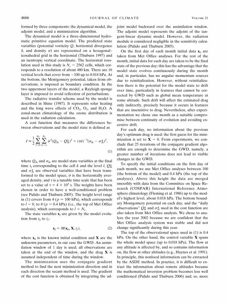
FIG. 3. (left) Zonal-mean GWD as a function of latitude and time at 0.24 hPa. A 10-day window averaging isused. The contour interval is 5 m s�1 day�1 (note resetting of grayscale). (right) Zonal-mean zonal wind at 0.24 hPa.The contour interval is 10 m s�1.

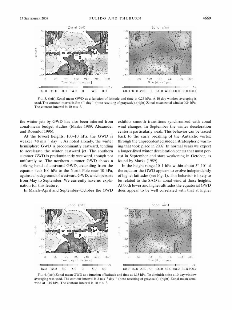
FIG. 4. (left) Zonal-mean GWD as a function of latitude and time at 1.15 hPa. To diminish noise a 10-day windowaveraging was used. The contour interval is 2 m s�1 day�1 (note resetting of grayscale). (right) Zonal-mean zonalwind at 1.15 hPa. The contour interval is 10 m s�1.


latitudes. The equatorial GWD behavior is discussed indetail later.

b. GWD seasonal variability

Figure 2 presents the monthly averaged zonal-meanGWD at three different latitudes: 60°N, 60°S, and at theequator. The patterns show similarities between theNorthern and Southern Hemisphere (left and middlepanels), such as the winter deceleration center at 0.24hPa with eastward acceleration below and the summerdeceleration above 1 hPa, with westward accelerationbelow. The dipolar structure at the end of boreal winter(left panel) is not found at austral winter. At lowerheights, below 10 hPa, there is some asymmetry be-tween the GWD in the two hemispheres, particularly inthe summer.

The right panel of Fig. 2 shows the evolution of themonthly averaged zonal wind (contours) and zonal-mean GWD (gray shading) at the equator. In this year,the westward phase of the QBO descends from about10 hPa in January to about 100 hPa in December. The

estimated GWD shows a westward forcing region thatdescends together with the zero zonal wind line. GWDvalues are about �0.5 m s�1 day�1. Similar tendencieshave been found by Alexander and Rosenlof (2003)using a zonal-mean budget study in a 6-yr period. Theirestimated values appear to be slightly smaller, around�0.25 m s�1 day�1. The SAO pattern is also capturedby ASDE: GWD above �5 hPa shows a semiannualcycle with peak eastward forcing of about 2.5 m s�1

day�1 and a weaker westward forcing of about �0.5m s�1 day�1.

Next we examine the GWD seasonal cycle as a func-tion of latitude. At 0.24 hPa, GWD shows an annualoscillation in extratropical regions (Fig. 3) with maxi-mum westward GWD during winter and maximumeastward GWD in summer, as expected. The winterdeceleration centers in both hemispheres show signifi-cant short time scale variability; a 10-day window aver-aging has been applied to make the contour plotsclearer—Fig. 6 shows a sample of unfiltered data. Thesummer deceleration centers, on the other hand, show

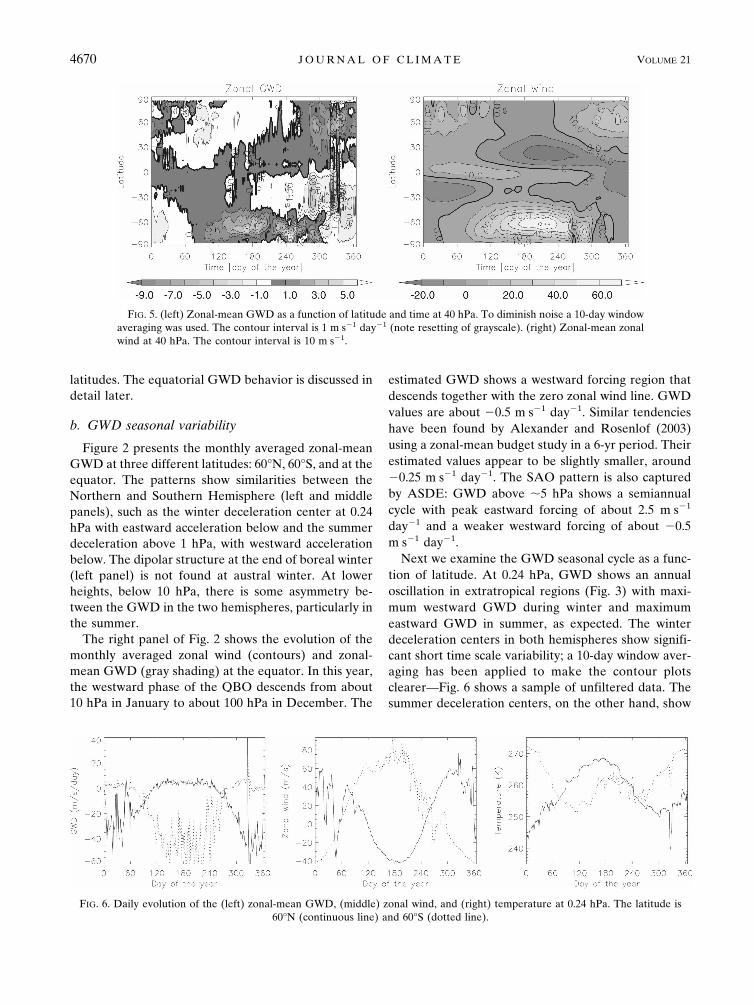
FIG. 5. (left) Zonal-mean GWD as a function of latitude and time at 40 hPa. To diminish noise a 10-day windowaveraging was used. The contour interval is 1 m s�1 day�1 (note resetting of grayscale). (right) Zonal-mean zonalwind at 40 hPa. The contour interval is 10 m s�1.

FIG. 6. Daily evolution of the (left) zonal-mean GWD, (middle) zonal wind, and (right) temperature at 0.24 hPa. The latitude is60°N (continuous line) and 60°S (dotted line).


much less short time scale variability. It is likely thatthese winter � summer differences in drag variabilityare related to winter � summer differences in zonalwind variability (right panel of Fig. 3) and in Rossbywave activity. GWD also appears to be sensitive to thestratospheric sudden warmings that occurred in bothhemispheres in 2002, (e.g., around day 25 and 55 in theNorthern Hemisphere and around day 265 in theSouthern Hemisphere). The estimated GWD itselfdoes not reverse sign at this altitude, though it does at0.40 hPa (not shown). The anomalous feature in thezonal drag on day 325 will be discussed further in thenext section. As already noted, maximum magnitudesin GWD in the winter hemisphere are located polewardof the winter jet, while maximum GWD values in thesummer hemispheres are located equatorward of thesummer jet.

At 1.15 hPa, the zonal GWD has predominantly thesame sign as the zonal wind (Fig. 4). The GWD exhibitshigh variability, particularly in the winter hemisphere.Typical magnitudes are much weaker than at 0.24 hPa,with peaks of 10 m s�1 day�1 in the winter hemisphere

and 4 m s�1 day�1 in the summer hemisphere. In thesummer hemisphere westward GWD appears to maxi-mize during the build-up of the summer jet. At theequator, there are latitudinally concentrated eastwardGWD centers. If they are believable (their scale is closeto the grid scale used in the ASDE model, though theyare consistent with the forcing required to drive theSAO), then it is likely that they are due to equatoriallytrapped waves such as Kelvin waves.

GWD at lower altitudes is quite noisy (Fig. 5). How-ever the sign of the GWD is predominantly such as toaccelerate the prevailing zonal jets. On the equator asthe zonal wind changes from eastward to westward,related to the descending QBO zero wind line shown inthe right panel of Fig. 2, the zonal drag also changesfrom eastward to westward. As already mentioned, theestimated forcing is in accord with that required todrive the QBO.

c. GWD day-to-day variability

The assimilation technique is able to estimate GWDwith a temporal resolution of the order of a day, which

FIG. 7. Daily evolution of the zonal-mean GWD (continuous line), zonal wind (dotted line) on the equator at (left) 0.24 hPa,(middle) 1.15 hPa, and (right) 40 hPa.

FIG. 8. (left) Zonal-mean GWD and (right) zonal-mean zonal wind on 26 Dec 2002. The contour intervals are10 m s�1 day�1 and 10 m s�1, respectively.


is the temporal resolution of the employed Met Officeanalysis. This enables us to study the day-to-day vari-ability of GWD.

The daily evolution of zonal-mean GWD at 60°N and60°S (Fig. 6) shows a relatively smooth evolution duringsummer but large-amplitude day-to-day variability in

winter. This feature is visible in both hemispheres andis correlated with the mean zonal flow, which is alsohighly variable in winter (middle panel of Fig. 6). Ingeneral, variations in the GWD are quite well anticor-related with variations in the zonal wind. For example,in the Northern Hemisphere the eastward zonal wind

FIG. 9. Monthly averaged mass-weighted height integral of the zonal GWD (contour interval is 0.01 N m�2, label units are in 0.01N m�2). Positive values are shaded.


decelerates sharply around day 25 and again aroundday 55, accompanied by sharp reductions in the west-ward GWD. In the Southern Hemisphere the zonalwind reverses from eastward to westward around day265 during the unusual sudden warming, and at thesame time the zonal GWD changes sign.

An anomalous peak is found in zonal GWD on day

325, that is, 21 November (left panel of Fig. 6). Thispeak coincides with a sharp drop in temperature ofabout 10 K in both hemispheres and a correspondingjump in the Northern Hemisphere jet strength. Thisunphysical behavior suggests a problem with the analy-sis data for that day.

On the equator, at 0.24 and 1 hPa the daily GWD

FIG. 10. As in Fig. 9 but of the meridional GWD.


shows considerable day-to-day variability superposedon a clear semiannual oscillation with an amplitude ofabout 5 m s�1 day�1 (left and middle panels in Fig. 7).At 40 hPa (right panel in Fig. 7) again there is consid-erable day-to-day variability, now superposed on a sys-tematic negative trend of �1.31 (m s�1 day�1) yr�1,which correlates with the QBO variation in zonal wind.There is also a negative trend at higher altitudes inaddition to the semiannual oscillation. The trend is�1.79 (m s�1 day�1) yr�1 at 0.24 hPa and �1.19 (m s�1

day�1) yr�1 at 1.15 hPa. With only one-year assimila-tion we are not able to assess the causes of these highaltitude trends and whether they are related to theQBO.

On 28 December 2002 a strong increasing of GWD isfound that reaches positive values, at 60°N and 0.24 hPa(Fig. 6). The GWD estimated for a previous day, 26December 2002, is shown in Fig. 8 in order to examinehow the transition occurs and its relation to the zonal-mean zonal wind. A tripolar structure is found at north-ern high latitudes, with eastward GWD at 0.7 hPa andwestward GWD both above and below. The highestdeceleration center remains at 0.24 hPa, even when thejet core is located much lower (Fig. 8, right panel). Asthe season evolves the westward GWD center at 0.24hPa weakens until it disappears, while the eastwardGWD center gets stronger. This could be evidence ofgravity wave source variability since the filteringmechanism of a constant isotropic gravity wave spec-trum cannot explain directly this behavior.

d. Horizontal GWD dependencies

The upward flux of zonal pseudomomentum at thebottom of the model, assuming the horizontal diver-gence of fluxes and fluxes at the top are negligible, isgiven by

Fb � ��b

�t

�Xx d�. �3

An analogous expression holds for the upward flux ofnorthward pseudomomentum. Thus, in principle, wecan obtain information on gravity wave sources fromvertical profiles of GWD. For this calculation we take t � (p � 0.24 hPa). Because the density � decreasesrapidly with altitude, the integral is dominated by thelower and middle stratosphere, and the results are in-sensitive to the exact location of the top boundary andthe neglect of top boundary fluxes. Drag values greaterthan about 1000 m s�1 day�1 would be needed above t

in order to make a significant difference to the columnintegrals; such values are beyond the extreme valuespredicted by current typical GWD schemes (e.g.,McLandress and Scinocca 2005).

The monthly mean estimated upward fluxes areshown in Figs. 9 and 10. Both components show thegreatest signals over land in the winter hemisphere. Thelargest zonal component is 0.09 N m�2 in August at�58.5° latitude, 85.5° longitude. Positive and negativevalues tend to occur together forming dipoles, whichtend to be aligned north–south in the zonal componentand east–west in the meridional component. Confi-dence in these results is limited because the verticalintegrals are dominated by the lowest altitudes in themodel domain where the estimated drag appears noisy.Several different mechanisms have been hypothesizedas potential tropospheric sources for gravity waves thatpropagate into the middle atmosphere, including orog-raphy, convection, and spontaneous emission, but thesesources have not been reliably quantified globally. Ourresults suggest some correlation with regions of largeorography, but are not clear enough to add much to thisdebate.

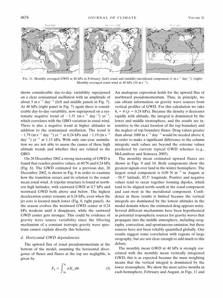
The monthly mean GWD at 40 hPa is strongly cor-related with the monthly mean vertically integratedGWD; this is as expected because the mass weightingmeans that the vertical integral is dominated by thelower stratosphere. We show the most active months ineach hemisphere, February and August, in Figs. 11 and

FIG. 11. Monthly averaged GWD at 40 hPa in February: (left) zonal and (middle) meridional component (1 m s�1 day�1). (right)Monthly averaged zonal wind at 40 hPa (10 m s�1).


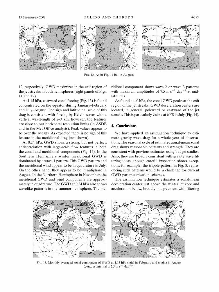
12, respectively. GWD maximizes in the exit region ofthe jet streaks in both hemispheres (right panels of Figs.11 and 12).

At 1.15 hPa, eastward zonal forcing (Fig. 13) is foundconcentrated on the equator during January–Februaryand July–August. The sign and latitudinal scale of thisdrag is consistent with forcing by Kelvin waves with avertical wavelength of 2–3 km; however, the featuresare close to our horizontal resolution limits (in ASDEand in the Met Office analysis). Peak values appear tobe over the oceans. As expected there is no sign of thisfeature in the meridional drag (not shown).

At 0.24 hPa, GWD shows a strong, but not perfect,anticorrelation with large-scale flow features in boththe zonal and meridional components (Fig. 14). In theSouthern Hemisphere winter meridional GWD isdominated by a wave 1 pattern. This GWD pattern andthe meridional wind appear to be in quadrature in July.On the other hand, they appear to be in antiphase inAugust. In the Northern Hemisphere in November, themeridional GWD and wind components are approxi-mately in quadrature. The GWD at 0.24 hPa also showswavelike patterns in the summer hemisphere. The me-

ridional component shows wave 2 or wave 3 patternswith maximum amplitudes of 7.5 m s�1 day�1 at mid-latitudes.

As found at 40 hPa, the zonal GWD peaks at the exitregion of the jet streaks. GWD deceleration centers arelocated, in general, poleward or eastward of the jetstreaks. This is particularly visible at 60°S in July (Fig. 14).

4. Conclusions

We have applied an assimilation technique to esti-mate gravity wave drag for a whole year of observa-tions. The seasonal cycle of estimated zonal-mean zonaldrag shows reasonable patterns and strength. They areconsistent with previous estimates using budget studies.Also, they are broadly consistent with gravity wave fil-tering ideas, though careful inspection shows excep-tions, for example, the tripole pattern in Fig. 8; repro-ducing such patterns would be a challenge for currentGWD parameterization schemes.

The assimilation technique estimates a zonal-meandeceleration center just above the winter jet core andacceleration below, broadly in agreement with filtering

FIG. 12. As in Fig. 11 but in August.

FIG. 13. Monthly averaged zonal component of GWD at 1.15 hPa (left) in February and (right) in August(contour interval is 2.5 m s�1 day�1).


mechanism predictions. These features have also beenfound with zonal-mean budget studies (Alexander andRosenlof 1996). The summer hemisphere also has azonal-mean deceleration center above the jet core and

acceleration below. A dipole pattern is present in thewinter–spring transition. The dipolar pattern is strongerin the Northern Hemisphere than in the SouthernHemisphere (see Figs. 1 and 2). The positive accelera-

FIG. 14. Monthly averaged fields at 0.24 hPa in (left) July, (middle) August, and (right) November. (from top to bottom) The fieldsare zonal and meridional GWD component (m s�1 day�1) and zonal and meridional wind component (m s�1).


tion center located below the winter deceleration cen-ter is strongest in January–February in the NorthernHemisphere. This behavior may be related to the struc-ture of the winter stratospheric jet, which is more tiltedand located in lower latitudes in the Northern Hemi-sphere.

The location of the winter zonal-mean decelerationcenter does not vary. In both northern and southernwinters, its center is at 63° and 0.24 hPa. Regrettably,the top of the observational space is at 0.4 hPa. Al-though the GWD components are estimated up to themodel top (about 0.018 hPa) the lack of observationsmay influence the height of the GWD center, especiallyin the summer where a higher deceleration center isexpected. The Southern Hemisphere was particularlyperturbed in 2002 so that Southern Hemisphere GWDpatterns were probably more similar than usual to thosein the Northern Hemisphere. In normal years we ex-pect stronger interhemispheric differences, as discussedby Shine (1989).

Although the winter deceleration centers in the twohemispheres are similar in magnitude and height, theirmaximum strength is attained in different seasons (Fig.1). In the Northern Hemisphere, the winter decelera-tion center maximizes in late autumn (November),while in the Southern Hemisphere it maximizes in win-ter (July).

The longitudinal structure of GWD appears to berelated to the wind patterns. However, their correlationis not unique. In the Southern Hemisphere lower me-sosphere we found that the large-scale wave patterns ofmeridional GWD and meridional wind are in antiphaseduring August, while they are in quadrature during Julyin the Southern Hemisphere and during February in theNorthern Hemisphere (Fig. 14).

The GWD is expected to be small near the equatorcompared with high latitude drag. Moreover, the errorsin drag estimation technique are expected to be largestthere (Pulido and Thuburn 2005). However, the resultsfor low latitudes appear realistic and are comparablewith those obtained by other techniques. The estimatedGWD in low latitudes shows that westward forcing de-scends together with the westward QBO phase. Athigher altitudes GWD shows a semiannual pattern thatis approximately out of phase with the SAO wind.

One outcome of this work is that we now have adatabase of daily three-dimensional drag fields to ac-company the Met Office wind and temperature analy-ses for the year 2002. We plan to use this database toestimate optimal parameters for one or more GWDparameterization schemes. Another follow-up study isan examination of the interannual variability of GWD,however GWD estimations may be affected by thechanges introduced in the Met Office assimilation sys-tem (among others, the implementation of a three-dimensional variational assimilation system in 2000 andof a gravity wave parameterization in 2003) so that theGWD sensitivity to these changes needs to be ad-dressed.

APPENDIX

Wave 2 Pattern in the Divergent GWD

For the reasons discussed in section 2, we have notshown results for the divergent component of GWD inthe main body of this paper. The divergent GWD esti-mated by ASDE gives a global-scale wave 2 pattern,which is particularly visible in the height-integrated di-vergent GWD. The wave pattern maximizes in Marchand September.

FIG. A1. Monthly averaged (left) temperature (contour interval 0.5 K) and (right) zonal wind (contour interval1 m s�1) differences at the model bottom layer between the control model evolution and Met Office analyses inMarch.


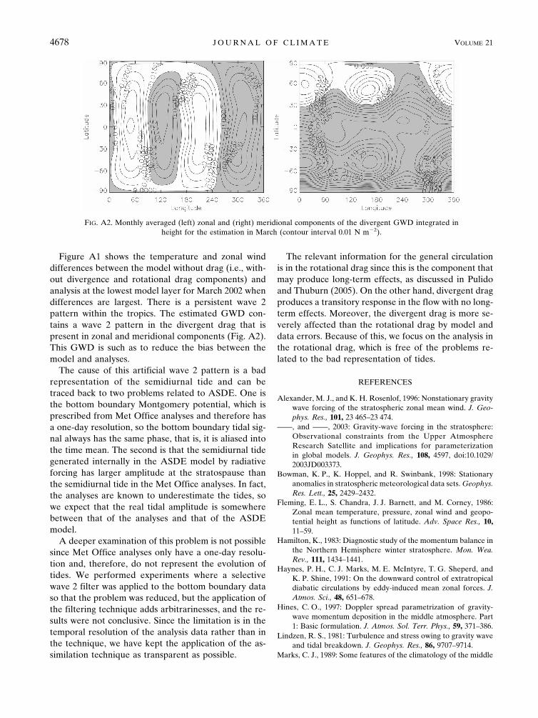
Figure A1 shows the temperature and zonal winddifferences between the model without drag (i.e., with-out divergence and rotational drag components) andanalysis at the lowest model layer for March 2002 whendifferences are largest. There is a persistent wave 2pattern within the tropics. The estimated GWD con-tains a wave 2 pattern in the divergent drag that ispresent in zonal and meridional components (Fig. A2).This GWD is such as to reduce the bias between themodel and analyses.

The cause of this artificial wave 2 pattern is a badrepresentation of the semidiurnal tide and can betraced back to two problems related to ASDE. One isthe bottom boundary Montgomery potential, which isprescribed from Met Office analyses and therefore hasa one-day resolution, so the bottom boundary tidal sig-nal always has the same phase, that is, it is aliased intothe time mean. The second is that the semidiurnal tidegenerated internally in the ASDE model by radiativeforcing has larger amplitude at the stratospause thanthe semidiurnal tide in the Met Office analyses. In fact,the analyses are known to underestimate the tides, sowe expect that the real tidal amplitude is somewherebetween that of the analyses and that of the ASDEmodel.

A deeper examination of this problem is not possiblesince Met Office analyses only have a one-day resolu-tion and, therefore, do not represent the evolution oftides. We performed experiments where a selectivewave 2 filter was applied to the bottom boundary dataso that the problem was reduced, but the application ofthe filtering technique adds arbitrarinesses, and the re-sults were not conclusive. Since the limitation is in thetemporal resolution of the analysis data rather than inthe technique, we have kept the application of the as-similation technique as transparent as possible.

The relevant information for the general circulationis in the rotational drag since this is the component thatmay produce long-term effects, as discussed in Pulidoand Thuburn (2005). On the other hand, divergent dragproduces a transitory response in the flow with no long-term effects. Moreover, the divergent drag is more se-verely affected than the rotational drag by model anddata errors. Because of this, we focus on the analysis inthe rotational drag, which is free of the problems re-lated to the bad representation of tides.

REFERENCES

Alexander, M. J., and K. H. Rosenlof, 1996: Nonstationary gravitywave forcing of the stratospheric zonal mean wind. J. Geo-phys. Res., 101, 23 465–23 474.

——, and ——, 2003: Gravity-wave forcing in the stratosphere:Observational constraints from the Upper AtmosphereResearch Satellite and implications for parameterizationin global models. J. Geophys. Res., 108, 4597, doi:10.1029/2003JD003373.

Bowman, K. P., K. Hoppel, and R. Swinbank, 1998: Stationaryanomalies in stratospheric meteorological data sets. Geophys.Res. Lett., 25, 2429–2432.

Fleming, E. L., S. Chandra, J. J. Barnett, and M. Corney, 1986:Zonal mean temperature, pressure, zonal wind and geopo-tential height as functions of latitude. Adv. Space Res., 10,11–59.

Hamilton, K., 1983: Diagnostic study of the momentum balance inthe Northern Hemisphere winter stratosphere. Mon. Wea.Rev., 111, 1434–1441.

Haynes, P. H., C. J. Marks, M. E. McIntyre, T. G. Sheperd, andK. P. Shine, 1991: On the downward control of extratropicaldiabatic circulations by eddy-induced mean zonal forces. J.Atmos. Sci., 48, 651–678.

Hines, C. O., 1997: Doppler spread parametrization of gravity-wave momentum deposition in the middle atmosphere. Part1: Basic formulation. J. Atmos. Sol. Terr. Phys., 59, 371–386.

Lindzen, R. S., 1981: Turbulence and stress owing to gravity waveand tidal breakdown. J. Geophys. Res., 86, 9707–9714.

Marks, C. J., 1989: Some features of the climatology of the middle

FIG. A2. Monthly averaged (left) zonal and (right) meridional components of the divergent GWD integrated inheight for the estimation in March (contour interval 0.01 N m�2).


atmosphere revealed by Nimbus 5 and 6. J. Atmos. Sci., 46,2485–2508.

McLandress, C., and J. F. Scinocca, 2005: The GCM response tocurrent parameterizations of nonorographic gravity wavedrag. J. Atmos. Sci., 62, 2394–2413.

Murgatroyd, R. J., and F. Singleton, 1961: Possible meridionalcirculations in the stratosphere and mesosphere. Quart. J.Roy. Meteor. Soc., 87, 125–135.

Pulido, M., and J. Thuburn, 2005: Gravity wave drag estimationfrom global analyses using variational data assimilation prin-ciples. I: Theory and implementation. Quart. J. Roy. Meteor.Soc., 131, 1821–1840.

——, and ——, 2006: Gravity wave drag estimation from globalanalyses using variational data assimilation principles. II: A

case study. Quart. J. Roy. Meteor. Soc., 132, 1527–1543,doi:10.1256/qj.05.43.

Shine, K., 1987: The middle atmosphere in the absence of dynami-cal heat fluxes. Quart. J. Roy. Meteor. Soc., 113, 603–633.

——, 1989: Sources and sinks of zonal momentum in the middleatmosphere diagnosed using the diabatic circulation. Quart.J. Roy. Meteor. Soc., 115, 265–292.

Swinbank, R., and A. O’Neill, 1994: A stratosphere tropospheredata assimilation system. Mon. Wea. Rev., 122, 686–702.

Thuburn, T., 1997: A PV-based shallow-water model on a hex-agonal–icosahedral grid. Mon. Wea. Rev., 125, 2328–2347.

Warner, C. D., and M. E. McIntyre, 1996: On the propagation anddissipation of gravity wave spectra through a realistic middleatmosphere. J. Atmos. Sci., 53, 3213–3235.


Documents

The Seasonal Cycle of Gravity Wave Drag in the Middle