The seasonal cycle amplitude of total column CO2: …prabir/papers/2011JD016124...The seasonal cycle amplitude of total column CO 2: Factors behind the model-observation mismatch Sourish

The seasonal cycle amplitude of total column CO2:Factors behind the model-observation mismatch

Sourish Basu,1 Sander Houweling,1,2 Wouter Peters,3 Colm Sweeney,4

Toshinobu Machida,5 Shamil Maksyutov,5 Prabir K. Patra,6 Ryu Saito,6

Frederic Chevallier,7 Yosuke Niwa,8 Hidekazu Matsueda,9 and Yousuke Sawa9

Received 18 April 2011; revised 23 September 2011; accepted 3 October 2011; published 15 December 2011.

[1] CO2 surface fluxes that are statistically consistent with surface layer measurementsof CO2, when propagated forward in time by atmospheric transport models,underestimate the seasonal cycle amplitude of total column CO2 in the northerntemperate latitudes by 1–2 ppm. In this paper we verify the systematic nature of thisunderestimation at a number of Total Carbon Column Observation Network (TCCON)stations by comparing their measurements with a number of transport models. Inparticular, at Park Falls, Wisconsin (United States), we estimate this mismatch to be1.4 ppm and try to attribute portions of this mismatch to different factors affecting thetotal column. We find that errors due to (1) the averaging kernel and prior profile usedin forward models, (2) water vapor in the model atmosphere, (3) incorrect verticaltransport by transport models in the free troposphere, (4) incorrect aging of air in transportmodels in the stratosphere, and (5) air mass dependence in TCCON data can explain up to1 ppm of this mismatch. The remaining 0.4 ppm mismatch is at the edge of the ≤0.4 ppmaccuracy requirement on satellite measurements to improve on our current estimate ofsurface fluxes. Uncertainties in the biosphere fluxes driving the transport models couldexplain a part of the remaining 0.4 ppm mismatch, implying that with corrections to thefactors behind the accounted-for 1 ppm underestimation, present inverse modelingframeworks could effectively assimilate satellite CO2 measurements.

Citation: Basu, S., et al. (2011), The seasonal cycle amplitude of total column CO2: Factors behind the model-observationmismatch, J. Geophys. Res., 116, D23306, doi:10.1029/2011JD016124.

1. Introduction

[2] An accurate estimate of the spatial distribution ofglobal CO2 surface flux and its annual and interannual vari-ation has been one of the holy grails of carbon cycle researchfor several decades. Such an estimate would, among otherthings, improve our ability to close regional and global car-bon budgets [Sarmiento and Gruber, 2002] and quantify theeffect of climate change on the size of terrestrial and oceaniccarbon sources and sinks [Le Quéré, 2007; Law et al., 2008a;Zickfeld et al., 2008]. Atmospheric inverse modeling of CO2,

which uses a global atmospheric transport model to arrive ata spatiotemporal distribution of surface fluxes that are sta-tistically consistent with measurements of CO2, is a power-ful top down method for estimating the sizes of those sourcesand sinks [Enting et al., 1995; Kaminski et al., 1999; Rayneret al., 1999; Bousquet et al., 2000; Krakauer et al., 2004;Baker et al., 2006; Rödenbeck et al., 2003]. State of the artCO2 inverse models today use surface measurements of CO2

taken at multiple stations across the globe [Tans et al., 1990;Conway et al., 1994; Bakwin et al., 1998]. The amount ofsurface data, however, is not enough to strongly constrain thespatiotemporal variability of surface fluxes. For example, theuncertainty in the mean annual CO2 flux from 1992 to 1996over South America is 0.64 Gt C/yr, compared to a meanannual flux of �0.24 Gt C/yr over that region [Gurney,2004]. Utilizing satellite measurements of total column CO2

from instruments such as GOSAT [Hamazaki et al., 2004]can theoretically better constrain the flux estimate andincrease its accuracy [Chevallier et al., 2007].[3] To be useful for atmospheric inversions, satellite

measurements need to be accurate enough to provide a tighterconstraint on surface fluxes than that already provided bysurface measurements. Specifically, to reduce the uncertain-ties in annual surface fluxes aggregated over 1000 �1000 km2 grid cells to 40% of their present values, systematic

1SRON Netherlands Institute for Space Research, Utrecht, Netherlands.2Institute for Marine and Atmospheric Research, Utrecht, Netherlands.3Department of Meteorology and Air Quality, Wageningen University

and Research Centre, Wageningen, Netherlands.4CIRES, University of Colorado at Boulder, Boulder, Colorado, USA.5National Institute for Environmental Studies, Tsukuba, Japan.6Research Institute for Global Change, JAMSTEC, Yokohama, Japan.7Laboratoire des Sciences du Climat et de l’Environnement, Gif-sur-

Yvette, France.8Atmosphere and Ocean Research Institute, University of Tokyo,

Kashiwa, Japan.9Geochemical Research Department, Meteorological Research Institute,

Tsukuba, Japan.

Copyright 2011 by the American Geophysical Union.0148-0227/11/2011JD016124

JOURNAL OF GEOPHYSICAL RESEARCH, VOL. 116, D23306, doi:10.1029/2011JD016124, 2011

D23306 1 of 14

http://dx.doi.org/10.1029/2011JD016124

errors on total column measurements must be less than0.4 ppm [Houweling et al., 2010; Ingmann et al., 2008;Chevallier et al., 2010]. However, such observational accu-racy will be wasted unless the transport models used foratmospheric inversions can simulate the total column CO2

mixing ratio (hereafter referred to as XCO2) equally accurately

when forced with “true” surface fluxes. To check whetheratmospheric transport models satisfy that requirement, weneed to check the XCO2

simulated by transport models againstobserved XCO2

.[4] This check cannot yet be performed against satellite

measurements of XCO2, since they themselves have yet to

meet the accuracy requirements mentioned above. To cali-brate satellite measurements, a ground-based global net-work (the Total Carbon Column Observation Network, orTCCON) of sun-facing Fourier transform spectrometers hasbeen built to provide continuous measurements of XCO2

andother trace gases [Toon et al., 2009; Wunch et al., 2011].We use TCCON measurements of XCO2

to validate XCO2

simulated by transport models. In particular, we look at theseasonal cycle of XCO2

as observed by TCCON and assimulated by models.[5] The seasonal cycle amplitude of XCO2

represents themost significant temporal variation of CO2 surface flux overannual time scales. Moreover, due to the relatively fast zonaltransport times compared to latitudinal transport times, theXCO2

seasonal cycle contains information about the season-ality of surface fluxes in the entire latitudinal band where thesite is located. Therefore, small variations in the seasonalamplitude of XCO2

can, when inverted, translate to largevariations in surface fluxes in the entire latitudinal band. Forexample, Yang et al. [2007] demonstrated that given anatmospheric transport model, a Net Ecosystem Exchange(NEE) in the northern temperate latitudes that is statisticallyconsistent with surface CO2 measurements needs to beincreased by �28% to be consistent with measurements thatdepend on CO2 higher up [Yang et al., 2007], specifically,XCO2

measurements at Park Falls and Kitt Peak, and short-term aircraft measurements at a few other sites. They cal-culated the NEE adjustment on the assumption that the entiremismatch in XCO2

observations stemmed from incorrectbiosphere fluxes fed to the transport models. However,specifying “true” biosphere fluxes to transport models willnot necessarily produce XCO2

consistent with observationsdue to shortcomings of the models. In this paper, we assessthe impact of the transport models themselves on the model-observation mismatch of XCO2

seasonal cycle amplitude.[6] We first confirm that at multiple TCCON sites in the

northern temperate latitudes, transport models systematicallysimulate a seasonal cycle amplitude of XCO2

that is lower by�2 ppm compared to observations. In doing this we dem-onstrate that the estimate of Yang et al. [2007], which wasbased on one TCCON site (Park Falls), one other XCO2

site(Kitt Peak), and a few short-term aircraft measurements,holds globally for multiple years in the northern temperatelatitudes. This mismatch could come from either observa-tional (TCCON) errors or model errors. Model errors comefrom errors in specifying the surface flux, errors in transport,and errors due to the large spatial resolution of the model,the so-called representation errors. Representation errorsalone, which can be estimated from modeled tracer gra-dients, are typically larger than reported errors in TCCON

data [Wunch et al., 2010]. Hence model errors are expectedto be much larger than TCCON measurement errors, and weconsider them to be the major factors behind the aforemen-tioned mismatch. Our goal therefore is to estimate parts ofthe mismatch coming from different model errors. Specifi-cally, we examine how transport models perform at differentaltitudes, and whether the majority of the mismatch comesfrom a few problematic pressure levels. Such a diagnosiswould provide pointers on how to fix the modeled transportat those levels without introducing errors at other levels.[7] Modeled CO2 concentrations in this paper come from

CarbonTracker release CT2010 and four transport modelsfrom the TRANSCOM 4 model intercomparison experimenttargeting the use of satellite measurements [Gurney, 2004;Patra et al., 2008; Saito et al., 2011]. The aim of theTRANSCOM experiment was to characterize the expectedvariability of total column CO2 over a range of spatiotem-poral scales, and to investigate how well these variations arereproduced by atmospheric transport models, given theiruncertainties. The experimental setup was the same as usedfor the TRANSCOM continuous experiment [Law et al.,2008b], except that three-dimensional concentration fieldswere stored at the time-step of the models. Furthermore,additional tracers were introduced replacing the CASA-derived terrestrial biosphere flux with hourly fluxes fromCarbonTracker [Peters et al., 2007], which were fed to themodels either hourly or as daily and monthly averages. Inthis paper we use output for the tracer corresponding tohourly CarbonTracker fluxes.[8] The structure of this manuscript is as follows. In

section 3 we demonstrate that transport models systemati-cally underestimate the seasonal cycle amplitude of XCO2

atmultiple TCCON sites. In section 4 we estimate the con-tributions to this mismatch from factors that affect the entirevertical column, namely the averaging kernel of TCCONinstruments, air mass–dependent corrections to TCCONobservations and atmospheric water column corrections tomodeled XCO2

. In section 5 we break the remaining mismatchdown into mismatches originating at different vertical levels.We use NOAA CMDL CO2 measurements in the surfacelayer, aircraft CO2 measurements over some locations in thelower troposphere, CONTRAIL CO2 measurements in thefree troposphere, and age-of-air experiments in the strato-sphere to examine model-observation mismatches at each ofthese layers. We summarize these comparisons in a “mis-match budget” in section 6. This budget falls short of themodel-TCCON mismatch seen in section 4, and in section 7we hypothesize on possible ways to close this budget.

2. Procedure for Data Analysis

2.1. Comparing Models to TCCON and Surface Data

[9] To construct seasonal cycles, a multiyear time series isdetrended and collapsed onto a single year. Throughout thispaper, CO2 concentrations were detrended by 2.01 ppm/yr.This trend was deduced from CO2 measurements at MaunaLoa, Hawaii, which, being in the middle of the ocean andfar away from anthropogenic and industrial influences, isrepresentative of the global growth rate. Although thelong-term trend since the start of the Mauna Loa CO2

record in 1974 is not linear, 2.01 ppm/yr is a very goodapproximation to the trend seen over the last ten years,

BASU ET AL.: SEASONAL CYCLE OF TOTAL COLUMN CO2 D23306D23306

2 of 14

which includes the time periods for our observations andmodel runs.[10] To compare with observed XCO2

, detrended modeldata, available as three dimensional concentration fields,were vertically averaged by weighing the mixing ratio ineach vertical layer by the air mass in the layer:

XCO2 ¼1

psurface

Xi

xiCO2pi � piþ1� �

; ð1Þ

xCO2

i being the CO2 mixing ratio in layer i above a certainsurface location. Layer i is between pressure levels pi andpi+1. The layer index increases from the ground up, so thesurface pressure is p0 = psurface. For comparing with sur-face measurements at locations with sampling towers,surface data at the highest tower levels were chosen toeliminate localized XCO2

fluctuations. For example, at ParkFalls we selected the tower data from 868 meters abovesea level (396 meters above the surface).[11] Ideally, the vertical averaging (equation (1)) of mod-

eled CO2 over a TCCON site should include the averagingkernel and prior profile used in the TCCON retrieval. Theaveraging kernel matrix A describes the sensitivity of theretrieved vertical profile xret to the true vertical profile xtrue

and the a priori vertical profile xprior [Rodgers, 2003; Deeteret al., 2003]

xreti ¼ xpriori þXj

Aij xtruej � xpriorj

� �; ð2Þ

where the subscripts refer to different vertical layers. For atotal column measurement, the matrix A is summed overdifferent layers to yield a total column averaging kernel[Deeter et al., 2007]. In section 4.2 we assess the impact ofincluding the averaging kernel on the modeled XCO2

seasonalcycle amplitude, as opposed to using a unit averaging kernel.[12] Most of the TCCON stations have come online only

in the past couple of years, while the model data used in thispaper span 2002–2003 (TRANSCOM 4 models) and 2001–2009 (CarbonTracker). Therefore exact cosampling ofmodels and observations was not always possible. ForFigure 2, we constructed 24 hr averages of the model data,whereas the TCCON daily averages, being daytime mea-surements, reflect daytime averages. This could give riseto some bias in the seasonal cycle, which we discuss insection 3. For a more detailed analysis later at the Park Falls,Wisconsin TCCON site, we sampled CarbonTracker exactlyat the TCCON measurement times and constructed averagesof all the measurements on a single day, thus precluding theaforementioned sampling bias. Such a cosampling was usedto construct, for example, Figure 3, and was used in ouranalysis from section 4 onward.[13] Since the XCO2

seasonal cycle amplitude does nothave a known significant trend, we expect the average sea-sonal cycle amplitude over multiple years at a location to bea good representation of the XCO2

seasonal cycle at thatlocation. Both modeled and observed data were binned into366 bins, with each bin corresponding to a day of year. Thedata inside each bin were averaged to yield a mean mixingratio for that day of year as well as its error. To assess theseasonal cycle amplitude, the daily averaged data weresmoothed using Loess smoothing [Cleveland et al., 1990].

The peak-to-peak values of the smoothed curves, i.e., thedifferences between the spring peaks and the summertroughs in the Northern Hemisphere, were used as estimatesof the respective seasonal cycle amplitudes.

2.2. Comparing Models to Aircraft Data

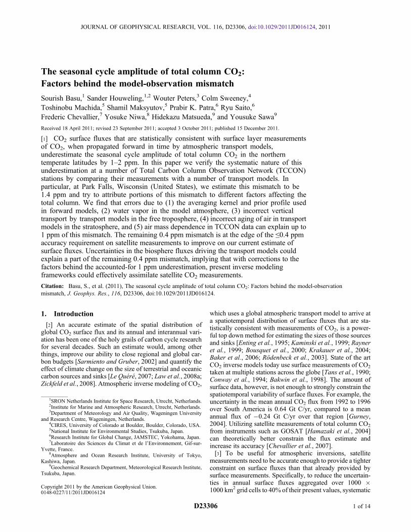
[14] In section 5.2 we compare CarbonTracker CO2 con-centrations with aircraft samples. All the aircraft data con-sidered were gathered between 2001 and 2008, the periodfor which we also possess CarbonTracker CO2 fields. Thisenabled us to sample CarbonTracker CO2 concentrations atthe same spatiotemporal locations as the aircraft samples.CarbonTracker uses pressure as a vertical coordinate,whereas certain aircraft campaigns used altitude. For aircraftdata reporting altitude but not pressure, radiosonde mea-surements over Lamont, Oklahoma, were used to translatebetween altitude and pressure levels. After cosampling, bothmodeled and observed data were binned into days of theyear as before, and averaged to yield a single value perlocation within some pressure interval for each day of theyear. The resulting averages were Loess smoothed to esti-mate the peak-to-peak seasonal cycle amplitudes.[15] In section 5.2 we estimate the contribution of differ-

ent vertical layers to the XCO2seasonal cycle amplitude. To

do this, we note that the extrema in XCO2do not occur at the

same time as the extrema in the individual layers (Figure 1).The amplitude in the seasonal cycle of XCO2

, hereafterreferred to as AX, can be written as

AX ¼ XCO2 tsð Þ � XCO2 tf� �

¼Xi

xiCO2tsð Þ p

i tsð Þ � piþ1 tsð Þpsurface tsð Þ � xiCO2

tf� � pi tf� �� piþ1 tf

� �psurface tf

� �" #

;

ð3Þ

where ts and tf denote the times for the spring peak and falltrough in XCO2

as read off from the modeled total column.Each term inside the summation can be thought of as thecontribution from one layer to AX. Specifically, the contri-bution of a layer between pressures p1 and p2 < p1 to AX is

DXCO2 p1; p2ð Þ ¼ xspring peakCO2

� xfall troughCO2

� �� p1 � p2

psurface: ð4Þ

So the cumulative contribution up to pressure level pi plottedin Figures 1 (middle) and 1 (right) isX

j;pj�pi

DXCO2 pj� 1; pj� �

=DXCO2 psurface; 0ð Þ: ð5Þ

We have plotted this measure of cumulative contribution asderived from CONTRAIL measurements in Figure 1 (mid-dle). This measure can be used to split the total column sea-sonal cycle amplitude into contributions coming fromdifferent layers, or to extrapolate partial column amplitudesinto total column amplitudes. For example, suppose that theXCO2

seasonal cycle amplitude at some location in thenorthern temperate latitude band is 1.56 ppm. According toFigure 1 (middle), 32% of this amplitude comes from layersbetween 730 hPa and 470 hPa (shaded interval). Therefore,the contribution of this partial column to the XCO2

seasonalcycle amplitude is 32% of 1.56 ppm, or 0.5 ppm. Alterna-tively, if we only had aircraft measurements between


3 of 14

730 hPa and 430 hPa, and if those measurements gave us apartial column seasonal cycle amplitude of 0.5 ppm, thenwe could estimate the XCO2

seasonal cycle amplitude to be1.56 ppm, under the assumption that the partial columnaircraft measurements have the same characteristics asCONTRAIL measurements.[16] Moreover, if we follow the procedure described

above with CarbonTracker CO2 fields to estimate the per-layer contribution to the modeled XCO2

seasonal cycle, wesee the same sort of graphs for cumulative contribution.Figure 1 (right) shows these graphs over multiple locationswhere we also have observational aircraft data. Briggsdale,Colorado, is a deviant site since it is a high-altitude site, witha lower surface pressure. If both observations and modelsfollow the contribution profile in Figure 1, then so shouldtheir difference. For example, over Park Falls, layers below400 hPa contribute 80% of both the modeled and observedseasonal cycle amplitude. Therefore a mismatch between thetwo over that partial column should also be 80% of themodel-observation mismatch in the XCO2

seasonal cycleamplitude.

[17] We have lower tropospheric aircraft CO2 measure-ments over multiple locations. In section 5.2.3 we use theprocedure detailed above to extrapolate the partial columnmismatches derived from those measurements to estimatemismatches in the XCO2

seasonal cycle amplitude. Forexample, over Estevan Point, British Columbia, we haveaircraft measurements of the CO2 vertical profile between981 hPa and 526 hPa. The seasonal cycle amplitude acrossthis partial column calculated from aircraft data is higherthan the modeled partial column seasonal cycle amplitude by0.27 ppm. According to Figure 1 (right), this pressureinterval contributes 60% of the total column seasonal cycleover Estevan Point. Therefore, the expected mismatch in thetotal column seasonal cycle is 0.45 ppm.

2.3. Estimating the Contribution of Surface FluxUncertainty

[18] In section 7.1 we estimate the impact surface fluxuncertainty on the XCO2

seasonal cycle amplitude. For thispurpose, optimized surface CO2 fluxes from six differentinversion frameworks were propagated forward using the

Figure 2. Seasonal cycle in the total column CO2mixing ratio at three different TCCON sites, all of whichare in the northern temperate latitudes. The green tract depicts the spread of four different TRANSCOM4 models (ACTM, LMDZ4, NIES05, TM5), the blue squares are from CarbonTracker 2010 posteriorCO2 fields, and the red circles are TCCON data. The dashed lines, meant as guides to the eye, areLoess-smoothed curves. TRANSCOM model data represent a run over 2002 and 2003, whereas Carbon-Tracker data are from 2001 to 2009.

Figure 1. (left) Seasonal cycles in individual pressure layers between 30°N and 60°N as sampled byCONTRAIL. The orange dashed lines are the days of the year corresponding to the springpeak and falltrough in XCO2

. For each level, or each colored curve, the contribution to the total column amplitude isthe difference between its values at the two orange lines. (middle) Summing up these contributions fromthe bottom up, we get the fractional contribution of all layers below a certain pressure level. For exam-ple, layers between 730 hPa and 470 hPa (shaded interval) contribute �32% of the seasonal cycle ampli-tude of XCO2

. (right) Modeled CarbonTracker CO2 profiles give similar cumulative contributionestimates at multiple sites.


4 of 14

TM5 transport model [Krol et al., 2005] on a 6° � 4° globalgrid with 25 s-pressure hybrid vertical levels from 1 January2003 to 31 December 2006. For each biosphere flux speci-fication XCO2

was calculated above the TCCON sites anddetrended, collapsed onto one year and smoothed accordingto the procedure of section 2.1. The peak-to-peak values ofthe resulting curves, as in section 2.1, were used as estimatesof the seasonal cycle amplitudes.

3. Results: TCCON Measurements VersusModels

[19] Following the procedure described in section 2.1, wecompared total column CO2 mixing ratio measurements fromTCCON sites (D. Wunch et al., The Total Carbon ColumnObserving Network, TCCON Data Archive, 2010, http://tccon.ipac.caltech.edu) [Toon et al., 2009] with total columnssimulated by four models from the TRANSCOM4 experiment(ACTM, LMDZ4, NIES05 and TM5) and CarbonTracker.The modeled XCO2

was calculated following equation (1).Figure 2 shows the spread of the four TRANSCOM models(green patch), TCCON daily averages (red circles) andCarbonTracker daily averages (blue squares).[20] As can be seen in Figure 2, while all the models can

reproduce the phasing of the seasonal cycles of XCO2at

multiple TCCON sites, they consistently underestimate theiramplitudes by 1–3 ppm. This underestimation is systematicand is seen at several TCCON sites, such as Park Falls(Figure 2, left), Lamont (Figure 2, middle) and Tsukuba(Figure 2, right).[21] Among all the TCCON sites in the northern temperate

latitudes, Park Falls has the longest period of data acquisi-tion, relatively few data gaps and a large seasonal cycle

amplitude, resulting in good statistics during analysis. It alsohas surface layer data from the NOAA flask sampling net-work and aircraft overflight data at different altitudes overseveral years. Therefore, henceforth we will focus on ParkFalls as a typical northern temperate TCCON station, toconstruct an “error budget” for the mismatch betweenTCCON-observed and modeled seasonal cycle amplitudes.[22] For the four TRANSCOM 4 models we have model

data for two years (2002 and 2003) whereas for Carbon-Tracker we have model data for nine years (2001 to 2009),which results in better statistics. According to Figure 2 andsimilar analyses over other TCCON sites, the seasonal cycleamplitude of XCO2

modeled by CarbonTracker is neitherconsistently higher nor consistently lower than other models,making its output fields good proxies for typical “modeldata.” Therefore, throughout the rest of this paper we willuse the term “model data” to refer to CarbonTracker data,unless otherwise specified. Later in section 8 we will discusshow our conclusions are affected by variations betweendifferent transport models.[23] Using CarbonTracker as a typical model has the

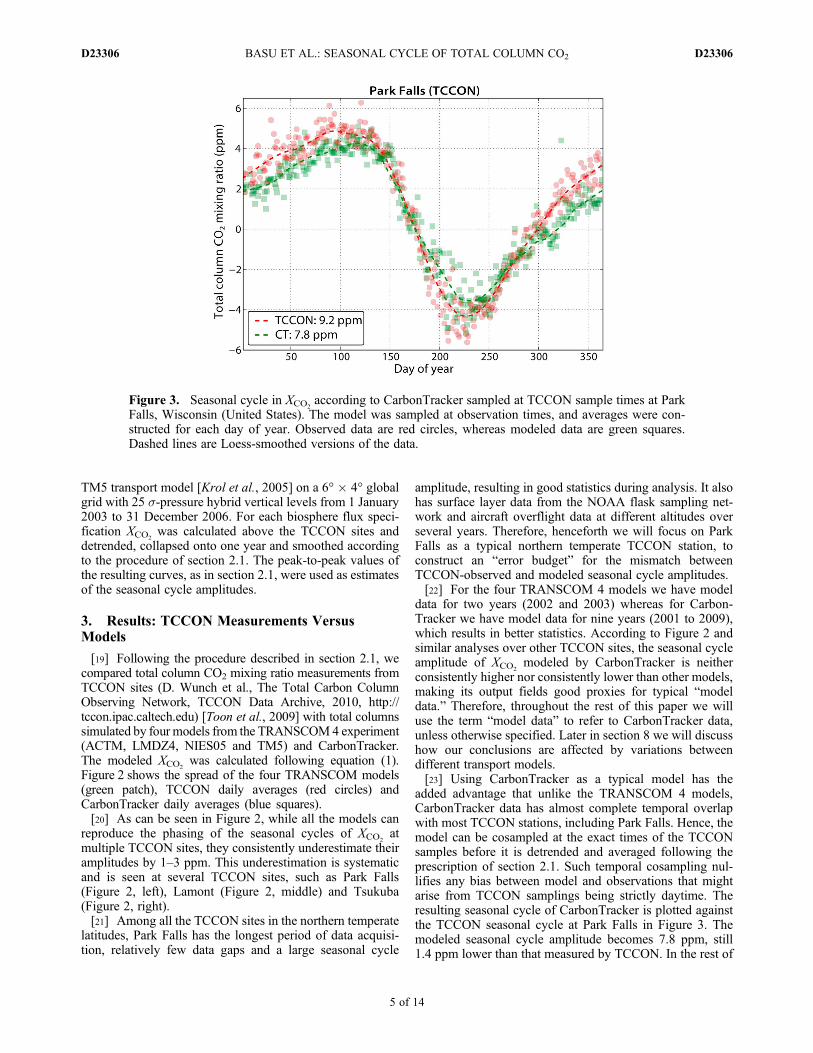
added advantage that unlike the TRANSCOM 4 models,CarbonTracker data has almost complete temporal overlapwith most TCCON stations, including Park Falls. Hence, themodel can be cosampled at the exact times of the TCCONsamples before it is detrended and averaged following theprescription of section 2.1. Such temporal cosampling nul-lifies any bias between model and observations that mightarise from TCCON samplings being strictly daytime. Theresulting seasonal cycle of CarbonTracker is plotted againstthe TCCON seasonal cycle at Park Falls in Figure 3. Themodeled seasonal cycle amplitude becomes 7.8 ppm, still1.4 ppm lower than that measured by TCCON. In the rest of

Figure 3. Seasonal cycle in XCO2according to CarbonTracker sampled at TCCON sample times at Park

Falls, Wisconsin (United States). The model was sampled at observation times, and averages were con-structed for each day of year. Observed data are red circles, whereas modeled data are green squares.Dashed lines are Loess-smoothed versions of the data.


5 of 14

this paper, we try to account quantitatively for the differentfactors behind this mismatch.

4. Factors Affecting the Whole Column

[24] As a first step toward understanding the mismatchesseen in Figures 2 and 3, we consider three factors that couldaffect XCO2

in models and measurements.

4.1. Water Vapor

[25] XCO2calculated by CarbonTracker is a “wet air” mole

fraction; that is, in the model, psurface of equation (1) is the

barometric pressure. By contrast, XCO2reported by TCCON

is the “dry air” mole fraction; that is, psurface excludes thesurface pressure due to the total water column in the atmo-sphere. Converting the modeled “wet air” XCO2

to a “dry air”XCO2

results in a small correction:

X dryCO2

¼ XwetCO2

� pwith watersurface

pwithout watersurface

: ð6Þ

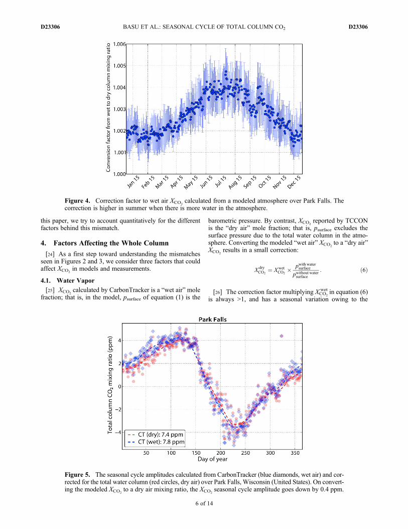
[26] The correction factor multiplying XCO2

wet in equation (6)is always >1, and has a seasonal variation owing to the

Figure 4. Correction factor to wet air XCO2calculated from a modeled atmosphere over Park Falls. The

correction is higher in summer when there is more water in the atmosphere.

Figure 5. The seasonal cycle amplitudes calculated from CarbonTracker (blue diamonds, wet air) and cor-rected for the total water column (red circles, dry air) over Park Falls, Wisconsin (United States). On convert-ing the modeled XCO2

to a dry air mixing ratio, the XCO2seasonal cycle amplitude goes down by 0.4 ppm.


6 of 14

seasonal variation of atmospheric water content. This factorwas calculated over Park Falls from ECMWF ERA-Interimwater columns and surface pressures for the entire TCCONoperation period. As can be seen in Figure 4, this factor has aseasonal variation, being higher in late summer (when thereis more water in the atmosphere) than early spring. So thecorrection of equation (6) raises the fall trough of XCO2

morethan it raises the spring maximum, decreasing the modeledseasonal cycle amplitude. This decrement over Park Falls, asseen in Figure 5, is 0.4 ppm, which is therefore the amount bywhich the model-observation mismatch is increased.

4.2. Averaging Kernel and Prior

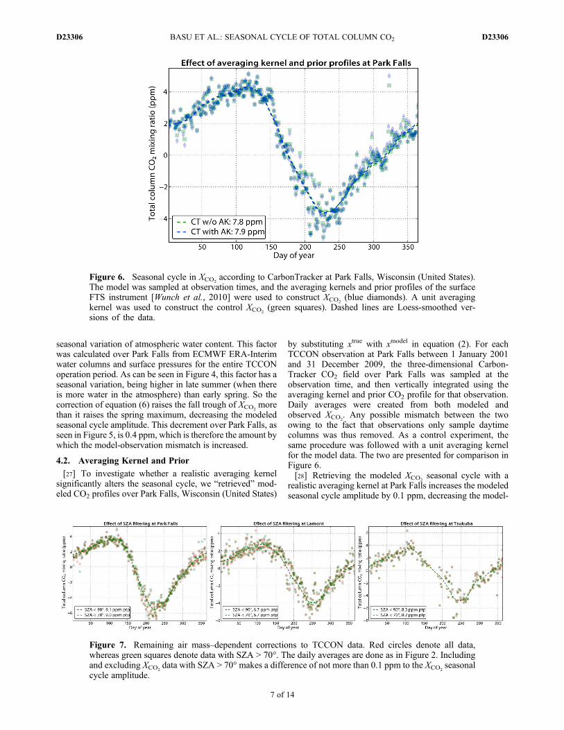
[27] To investigate whether a realistic averaging kernelsignificantly alters the seasonal cycle, we “retrieved” mod-eled CO2 profiles over Park Falls, Wisconsin (United States)

by substituting xtrue with xmodel in equation (2). For eachTCCON observation at Park Falls between 1 January 2001and 31 December 2009, the three-dimensional Carbon-Tracker CO2 field over Park Falls was sampled at theobservation time, and then vertically integrated using theaveraging kernel and prior CO2 profile for that observation.Daily averages were created from both modeled andobserved XCO2

. Any possible mismatch between the twoowing to the fact that observations only sample daytimecolumns was thus removed. As a control experiment, thesame procedure was followed with a unit averaging kernelfor the model data. The two are presented for comparison inFigure 6.[28] Retrieving the modeled XCO2

seasonal cycle with arealistic averaging kernel at Park Falls increases the modeledseasonal cycle amplitude by 0.1 ppm, decreasing the model-

Figure 6. Seasonal cycle in XCO2according to CarbonTracker at Park Falls, Wisconsin (United States).

The model was sampled at observation times, and the averaging kernels and prior profiles of the surfaceFTS instrument [Wunch et al., 2010] were used to construct XCO2

(blue diamonds). A unit averagingkernel was used to construct the control XCO2

(green squares). Dashed lines are Loess-smoothed ver-sions of the data.

Figure 7. Remaining air mass–dependent corrections to TCCON data. Red circles denote all data,whereas green squares denote data with SZA > 70°. The daily averages are done as in Figure 2. Includingand excluding XCO2

data with SZA > 70° makes a difference of not more than 0.1 ppm to the XCO2seasonal

cycle amplitude.


7 of 14

observation mismatch by the same amount. We verified thatthe correction due to the averaging kernel and prior atLamont was 0.1 ppm as well (not shown). Since the aver-aging kernels and prior profiles for TCCON CO2 are similaracross all the sites [Wunch et al., 2010], we expect the effectof including the averaging kernel to be similar at sites in thenorthern temperate latitudes.

4.3. Air Mass Dependence of TCCON Data

[29] The total column CO2 retrieved by a TCCON instru-ment is corrected for any air mass dependency in publishedTCCON data sets [Deutscher et al., 2010]. This correctionis a function of the solar zenith angle (SZA), which has aseasonal variation, causing any uncorrected air massdependence to influence the observed seasonal cycleamplitude. The air mass–dependent correction is quite small;XCO2

retrieved from the same vertical profile is higher by�1% at 20° SZA compared to 80° SZA [Wunch et al., 2011].Therefore any uncorrected air mass–dependence aliasing intothe seasonal cycle is expected to be even smaller [Wunchet al., 2010, 2011]. To quantify the influence of remainingair mass–dependent corrections on the seasonal cycle ampli-tude, we checked the impact of excluding TCCON data withSZA > 70° where air mass–dependent corrections are mostsignificant (P. Wennberg, personal communication, 2010).As can be seen in Figure 7, if we exclude data withSZA > 70°, the impact on theXCO2

seasonal cycle amplitude isminimal. For future use we note that at Park Falls this filteringdecreases the observed amplitude by 0.1 ppm, decreasing themodel-observation mismatch by the same amount.

5. Vertical Profile of the Mismatch

[30] In section 4 we looked at three factors that affect thetotal atmospheric column, and saw that they are not suffi-cient to explain the observed mismatch seen in Figure 3.This raises the question whether there are certain layers inthe atmosphere that generate the majority of the mismatch.Aircraft measurements of CO2 at different heights and dif-ferent seasons can be used to construct a seasonal cycleabove the surface, which can then be compared with themodeled seasonal cycle. However, aircraft measurements are

not total column measurements, and to assess the impact ofmismatches between aircraft CO2 samples and Carbon-Tracker CO2 fields, we must evaluate how such mismatchesaffect the total column seasonal cycle amplitude. Carbon-Tracker CO2 fields, it should be noted, are optimized againstsurface layer CO2 measurements but not total column oraircraft CO2 measurements.[31] In section 2.2 we detailed how to calculate the con-

tribution of different vertical layers to the seasonal cycle inXCO2

, and also how to estimate the model-measurementmismatch in the XCO2

seasonal cycle amplitude from mea-surements in a partial column. We will now look at howmodeled CO2 differs from measured CO2 at differentpressure levels. Using graphs from Figures 1 (middle) and1 (right), we will estimate the impact of these individualmismatches on the total column mismatch.

5.1. Surface Layer: NOAA CMDL

[32] We compared in situ and flask measurements of CO2

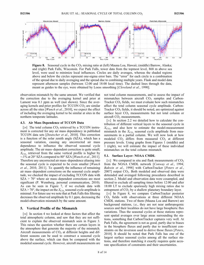
from the NOAA CMDL network [Conway et al., 1994;Bakwin et al., 1998] with CarbonTracker [Peters et al.,2007] output CO2. Both modeled and observed data weredetrended and averaged following procedures described insection 2. Model and observation data were cosampled, andfiltered to exclude all sampling times before 12:00 and after18:00 LT to exclude spuriously high mixing ratios due toentrapment of CO2 by a shallow planetary boundary layer.[33] In Figure 8, we compare CarbonTracker posterior

CO2 fields with observations at three different NOAACMDL stations. Two of them (Mauna Loa and Barrow) arebackground stations, i.e., they are not near anthropogenicsources and their localities do not have large biospheric fluxvariations. Thus the seasonal cycles at those stations repre-sent spatial averages over large areas surrounding the sta-tions, something that CarbonTracker captures very well. AtPark Falls, the agreement is not as good, partly due to biasesin the biosphere fluxes and partly due to insufficient con-straints on the inversion used to derive those fluxes [Peters,2010]. It should be noted that Park Falls has one of thelargest surface seasonal cycles among all the surface sta-tions, and therefore matching it exactly requires quite accu-rate specification of constraints and their uncertainties.

Figure 8. Seasonal cycle in the CO2 mixing ratio at (left) Mauna Loa, Hawaii; (middle) Barrow, Alaska;and (right) Park Falls, Wisconsin. For Park Falls, tower data from the topmost level, 868 m above sealevel, were used to minimize local influences. Circles are daily averages, whereas the shaded regionsabove and below the circles represent one-sigma error bars. The “error” for each circle is a combinationof the spread due to daily averaging and the spread due to combining multiple years. Flask and model datarepresent afternoon samples (between 12:00 and 18:00 local time). The dashed lines through the data,meant as guides to the eye, were obtained by Loess smoothing [Cleveland et al., 1990].


8 of 14

[34] From Figure 8 we conclude that modeled CO2 at thesurface layer in the northern temperate latitudes faithfullyreproduces large-scale spatiotemporal features seen inobservations. There are XCO2

measurements, surface mea-surements as well as aircraft measurements at Park Falls.Therefore, we will use Park Falls as a validation station formodeled CO2, i.e., we will compare modeled CO2 at variousvertical layers over Park Falls with observed CO2 to drawconclusions about the performance of transport models atvarious heights, and the contributions from different heightsto the mismatch of Figure 3, which will be summarized insection 6.

5.2. Free Troposphere: Aircraft Measurements

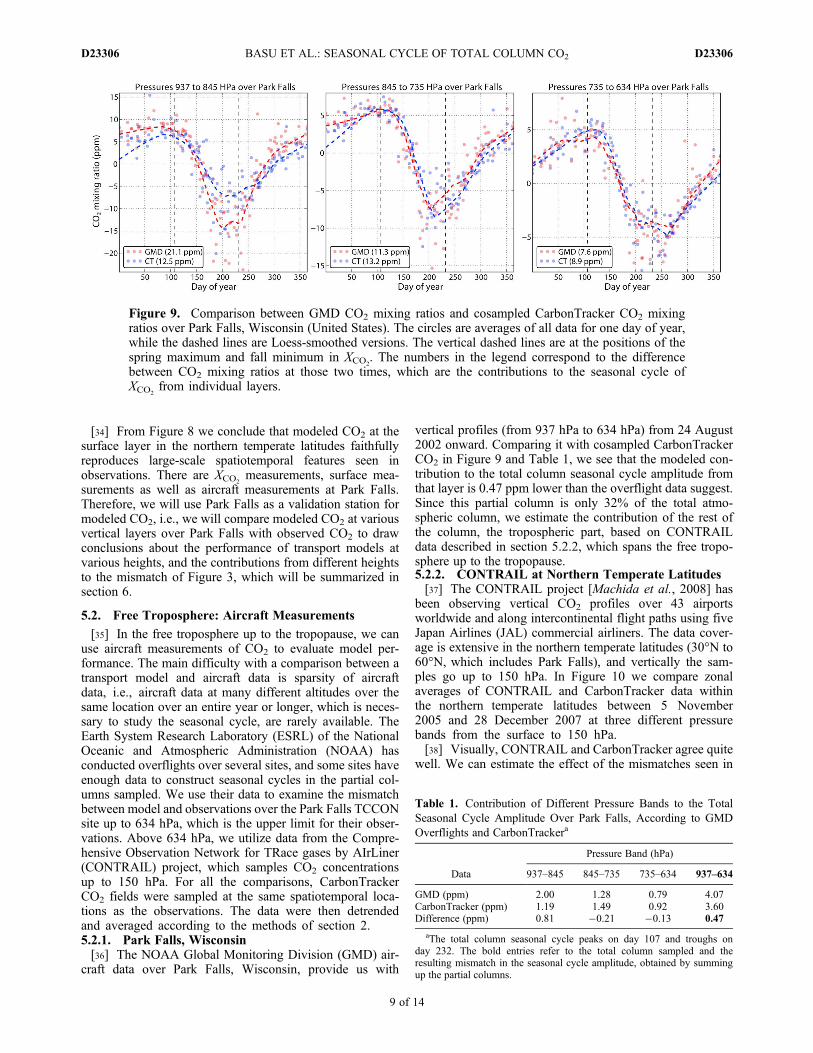
[35] In the free troposphere up to the tropopause, we canuse aircraft measurements of CO2 to evaluate model per-formance. The main difficulty with a comparison between atransport model and aircraft data is sparsity of aircraftdata, i.e., aircraft data at many different altitudes over thesame location over an entire year or longer, which is neces-sary to study the seasonal cycle, are rarely available. TheEarth System Research Laboratory (ESRL) of the NationalOceanic and Atmospheric Administration (NOAA) hasconducted overflights over several sites, and some sites haveenough data to construct seasonal cycles in the partial col-umns sampled. We use their data to examine the mismatchbetween model and observations over the Park Falls TCCONsite up to 634 hPa, which is the upper limit for their obser-vations. Above 634 hPa, we utilize data from the Compre-hensive Observation Network for TRace gases by AIrLiner(CONTRAIL) project, which samples CO2 concentrationsup to 150 hPa. For all the comparisons, CarbonTrackerCO2 fields were sampled at the same spatiotemporal loca-tions as the observations. The data were then detrendedand averaged according to the methods of section 2.5.2.1. Park Falls, Wisconsin[36] The NOAA Global Monitoring Division (GMD) air-

craft data over Park Falls, Wisconsin, provide us with

vertical profiles (from 937 hPa to 634 hPa) from 24 August2002 onward. Comparing it with cosampled CarbonTrackerCO2 in Figure 9 and Table 1, we see that the modeled con-tribution to the total column seasonal cycle amplitude fromthat layer is 0.47 ppm lower than the overflight data suggest.Since this partial column is only 32% of the total atmo-spheric column, we estimate the contribution of the rest ofthe column, the tropospheric part, based on CONTRAILdata described in section 5.2.2, which spans the free tropo-sphere up to the tropopause.5.2.2. CONTRAIL at Northern Temperate Latitudes[37] The CONTRAIL project [Machida et al., 2008] has

been observing vertical CO2 profiles over 43 airportsworldwide and along intercontinental flight paths using fiveJapan Airlines (JAL) commercial airliners. The data cover-age is extensive in the northern temperate latitudes (30°N to60°N, which includes Park Falls), and vertically the sam-ples go up to 150 hPa. In Figure 10 we compare zonalaverages of CONTRAIL and CarbonTracker data withinthe northern temperate latitudes between 5 November2005 and 28 December 2007 at three different pressurebands from the surface to 150 hPa.[38] Visually, CONTRAIL and CarbonTracker agree quite

well. We can estimate the effect of the mismatches seen in

Figure 9. Comparison between GMD CO2 mixing ratios and cosampled CarbonTracker CO2 mixingratios over Park Falls, Wisconsin (United States). The circles are averages of all data for one day of year,while the dashed lines are Loess-smoothed versions. The vertical dashed lines are at the positions of thespring maximum and fall minimum in XCO2

. The numbers in the legend correspond to the differencebetween CO2 mixing ratios at those two times, which are the contributions to the seasonal cycle ofXCO2

from individual layers.

Table 1. Contribution of Different Pressure Bands to the TotalSeasonal Cycle Amplitude Over Park Falls, According to GMDOverflights and CarbonTrackera

Data

Pressure Band (hPa)

937–845 845–735 735–634 937–634

GMD (ppm) 2.00 1.28 0.79 4.07CarbonTracker (ppm) 1.19 1.49 0.92 3.60Difference (ppm) 0.81 �0.21 �0.13 0.47

aThe total column seasonal cycle peaks on day 107 and troughs onday 232. The bold entries refer to the total column sampled and theresulting mismatch in the seasonal cycle amplitude, obtained by summingup the partial columns.


9 of 14

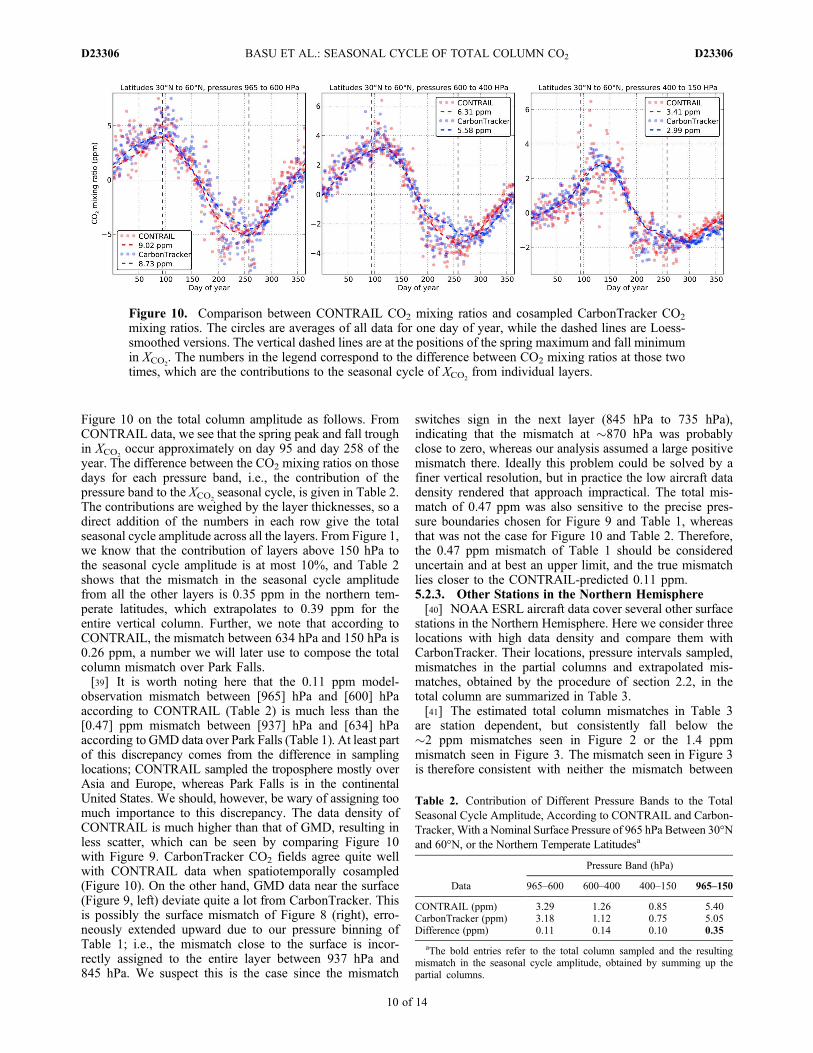
Figure 10 on the total column amplitude as follows. FromCONTRAIL data, we see that the spring peak and fall troughin XCO2

occur approximately on day 95 and day 258 of theyear. The difference between the CO2 mixing ratios on thosedays for each pressure band, i.e., the contribution of thepressure band to the XCO2

seasonal cycle, is given in Table 2.The contributions are weighed by the layer thicknesses, so adirect addition of the numbers in each row give the totalseasonal cycle amplitude across all the layers. From Figure 1,we know that the contribution of layers above 150 hPa tothe seasonal cycle amplitude is at most 10%, and Table 2shows that the mismatch in the seasonal cycle amplitudefrom all the other layers is 0.35 ppm in the northern tem-perate latitudes, which extrapolates to 0.39 ppm for theentire vertical column. Further, we note that according toCONTRAIL, the mismatch between 634 hPa and 150 hPa is0.26 ppm, a number we will later use to compose the totalcolumn mismatch over Park Falls.[39] It is worth noting here that the 0.11 ppm model-

observation mismatch between [965] hPa and [600] hPaaccording to CONTRAIL (Table 2) is much less than the[0.47] ppm mismatch between [937] hPa and [634] hPaaccording to GMD data over Park Falls (Table 1). At least partof this discrepancy comes from the difference in samplinglocations; CONTRAIL sampled the troposphere mostly overAsia and Europe, whereas Park Falls is in the continentalUnited States. We should, however, be wary of assigning toomuch importance to this discrepancy. The data density ofCONTRAIL is much higher than that of GMD, resulting inless scatter, which can be seen by comparing Figure 10with Figure 9. CarbonTracker CO2 fields agree quite wellwith CONTRAIL data when spatiotemporally cosampled(Figure 10). On the other hand, GMD data near the surface(Figure 9, left) deviate quite a lot from CarbonTracker. Thisis possibly the surface mismatch of Figure 8 (right), erro-neously extended upward due to our pressure binning ofTable 1; i.e., the mismatch close to the surface is incor-rectly assigned to the entire layer between 937 hPa and845 hPa. We suspect this is the case since the mismatch

switches sign in the next layer (845 hPa to 735 hPa),indicating that the mismatch at �870 hPa was probablyclose to zero, whereas our analysis assumed a large positivemismatch there. Ideally this problem could be solved by afiner vertical resolution, but in practice the low aircraft datadensity rendered that approach impractical. The total mis-match of 0.47 ppm was also sensitive to the precise pres-sure boundaries chosen for Figure 9 and Table 1, whereasthat was not the case for Figure 10 and Table 2. Therefore,the 0.47 ppm mismatch of Table 1 should be considereduncertain and at best an upper limit, and the true mismatchlies closer to the CONTRAIL-predicted 0.11 ppm.5.2.3. Other Stations in the Northern Hemisphere[40] NOAA ESRL aircraft data cover several other surface

stations in the Northern Hemisphere. Here we consider threelocations with high data density and compare them withCarbonTracker. Their locations, pressure intervals sampled,mismatches in the partial columns and extrapolated mis-matches, obtained by the procedure of section 2.2, in thetotal column are summarized in Table 3.[41] The estimated total column mismatches in Table 3

are station dependent, but consistently fall below the�2 ppm mismatches seen in Figure 2 or the 1.4 ppmmismatch seen in Figure 3. The mismatch seen in Figure 3is therefore consistent with neither the mismatch between

Figure 10. Comparison between CONTRAIL CO2 mixing ratios and cosampled CarbonTracker CO2

mixing ratios. The circles are averages of all data for one day of year, while the dashed lines are Loess-smoothed versions. The vertical dashed lines are at the positions of the spring maximum and fall minimumin XCO2

. The numbers in the legend correspond to the difference between CO2 mixing ratios at those twotimes, which are the contributions to the seasonal cycle of XCO2

from individual layers.

Table 2. Contribution of Different Pressure Bands to the TotalSeasonal Cycle Amplitude, According to CONTRAIL and Carbon-Tracker, With a Nominal Surface Pressure of 965 hPa Between 30°Nand 60°N, or the Northern Temperate Latitudesa

Data

Pressure Band (hPa)

965–600 600–400 400–150 965–150

CONTRAIL (ppm) 3.29 1.26 0.85 5.40CarbonTracker (ppm) 3.18 1.12 0.75 5.05Difference (ppm) 0.11 0.14 0.10 0.35

aThe bold entries refer to the total column sampled and the resultingmismatch in the seasonal cycle amplitude, obtained by summing up thepartial columns.


10 of 14

CarbonTracker and CONTRAIL data (which covers up to150 hPa globally) nor the mismatch between CarbonTrackerand NOAA ESRL aircraft data over specific sites. Accordingto both those comparisons, CarbonTracker should be betterat estimating the seasonal cycle amplitude than suggested byFigures 2 and 3.

5.3. Age of Air in the Free Troposphereand Stratosphere

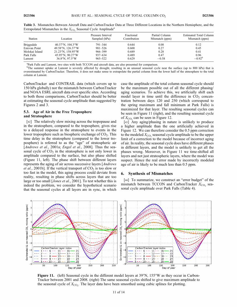
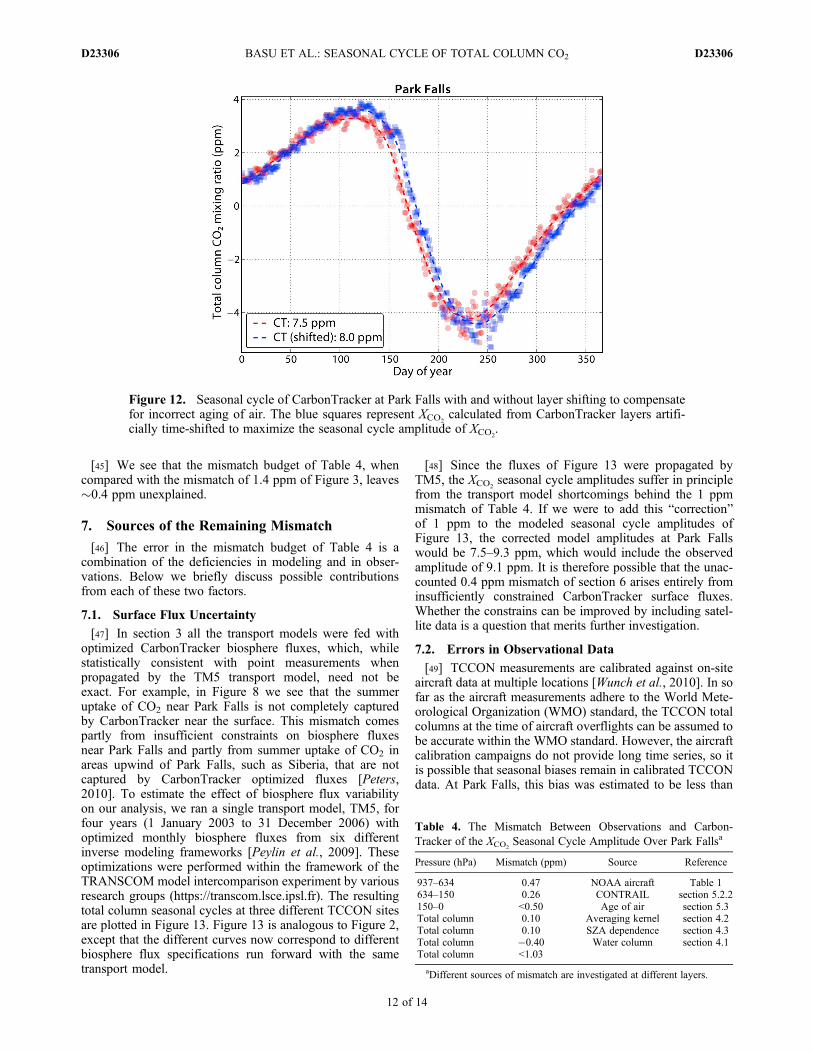
[42] The relatively slow mixing across the tropopause andin the stratosphere, compared to the troposphere, gives riseto a delayed response in the stratosphere to events in thelower troposphere such as biospheric exchange of CO2. Thistime delay in the stratosphere (compared to the lower tro-posphere) is referred to as the “age” of stratospheric air[Andrews et al., 2001a; Engel et al., 2008]. Thus the sea-sonal cycle of CO2 in the stratosphere is not only lower inamplitude compared to the surface, but also phase shifted(Figure 11, left). The phase shift between different layersrepresents the aging of air across successive layers [Andrewset al., 2001b]. If the vertical transport of CO2 is too slow ortoo fast in the model, this aging process could deviate fromreality, resulting in phase shifts across layers that are toolarge or too small [Jones et al., 2001]. To test whether this isindeed the problem, we consider the hypothetical scenariothat the seasonal cycles at all layers are in sync, in which

case the amplitude of the total column seasonal cycle shouldbe the maximum possible out of all the different phasing/aging scenarios. To achieve this, we artificially shift eachmodel layer in time until the difference in CO2 concen-tration between days 120 and 250 (which correspond tothe spring maximum and fall minimum at Park Falls) ismaximized for that layer. The resulting seasonal cycles canbe seen in Figure 11 (right), and the resulting seasonal cycleof XCO2

can be seen in Figure 12.[43] Any aging/phasing in nature is unlikely to produce

a higher amplitude than the one artificially achieved inFigure 12. We can therefore consider the 0.5 ppm correctionto the modeled XCO2

seasonal cycle amplitude to be the upperlimit of a correction to the model because of incorrect agingof air. In reality, the seasonal cycle does have different phasesin different layers, and the model is unlikely to get all thephases wrong. Moreover, in Figure 11 we time-shifted alllayers and not just stratospheric layers, where the model wassuspect. Hence the real error made by incorrectly modeledage of air is likely to be much less than 0.5 ppm.

6. Synthesis of Mismatches

[44] To summarize, we construct an “error budget” of themismatch between TCCON and CarbonTracker XCO2

sea-sonal cycle amplitude over Park Falls (Table 4).

Table 3. Mismatches Between Aircraft Data and CarbonTracker Data at Three Different Locations in the Northern Hemisphere, and theExtrapolated Mismatches in the XCO2

Seasonal Cycle Amplitudea

Station LocationPressure IntervalSampled (hPa)

FractionalContribution

Partial ColumnMismatch (ppm)

Estimated Total ColumnMismatch (ppm)

Briggsdale 40.37°N, 104.3°W 791–344 0.644 0.08 0.12Estevan Point 49.58°N, 126.37°W 981–526 0.600 0.27 0.45Molokai Island 21.23°N, 158.95°W 966–399 0.689 0.28 0.41Park Falls 45.95°N, 90.27°W 937–634 0.489 0.47 0.96Lamont 36.8°N, 97.5°W 965–522 0.629 �0.58 �0.92b

aPark Falls and Lamont, two sites with both TCCON and aircraft data, are also presented for comparison.bThe summer uptake at Lamont is severely affected by drought, resulting in an unusual seasonal cycle near the surface (up to 800 hPa) that is

overestimated by CarbonTracker. Therefore, it does not make sense to extrapolate the partial column from the lower half of the atmosphere to the totalcolumn at Lamont.

Figure 11. (left) Seasonal cycle in the different model layers at 39°N, 155°W as they occur in Carbon-Tracker between 2001 and 2008. (right) The same seasonal cycles shifted to give maximum amplitude tothe seasonal cycle of XCO2

. The layer data have been smoothed using cubic splines for plotting.


11 of 14

[45] We see that the mismatch budget of Table 4, whencompared with the mismatch of 1.4 ppm of Figure 3, leaves�0.4 ppm unexplained.

7. Sources of the Remaining Mismatch

[46] The error in the mismatch budget of Table 4 is acombination of the deficiencies in modeling and in obser-vations. Below we briefly discuss possible contributionsfrom each of these two factors.

7.1. Surface Flux Uncertainty

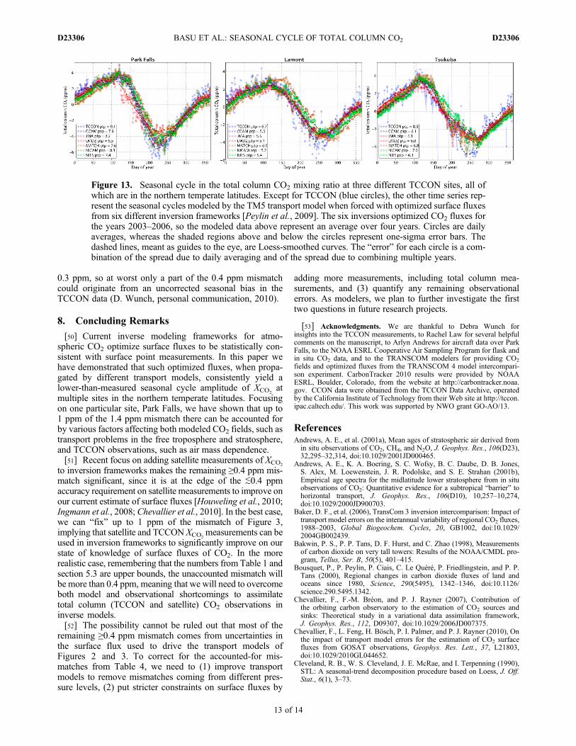
[47] In section 3 all the transport models were fed withoptimized CarbonTracker biosphere fluxes, which, whilestatistically consistent with point measurements whenpropagated by the TM5 transport model, need not beexact. For example, in Figure 8 we see that the summeruptake of CO2 near Park Falls is not completely capturedby CarbonTracker near the surface. This mismatch comespartly from insufficient constraints on biosphere fluxesnear Park Falls and partly from summer uptake of CO2 inareas upwind of Park Falls, such as Siberia, that are notcaptured by CarbonTracker optimized fluxes [Peters,2010]. To estimate the effect of biosphere flux variabilityon our analysis, we ran a single transport model, TM5, forfour years (1 January 2003 to 31 December 2006) withoptimized monthly biosphere fluxes from six differentinverse modeling frameworks [Peylin et al., 2009]. Theseoptimizations were performed within the framework of theTRANSCOM model intercomparison experiment by variousresearch groups (https://transcom.lsce.ipsl.fr). The resultingtotal column seasonal cycles at three different TCCON sitesare plotted in Figure 13. Figure 13 is analogous to Figure 2,except that the different curves now correspond to differentbiosphere flux specifications run forward with the sametransport model.

[48] Since the fluxes of Figure 13 were propagated byTM5, the XCO2

seasonal cycle amplitudes suffer in principlefrom the transport model shortcomings behind the 1 ppmmismatch of Table 4. If we were to add this “correction”of 1 ppm to the modeled seasonal cycle amplitudes ofFigure 13, the corrected model amplitudes at Park Fallswould be 7.5–9.3 ppm, which would include the observedamplitude of 9.1 ppm. It is therefore possible that the unac-counted 0.4 ppm mismatch of section 6 arises entirely frominsufficiently constrained CarbonTracker surface fluxes.Whether the constrains can be improved by including satel-lite data is a question that merits further investigation.

7.2. Errors in Observational Data

[49] TCCON measurements are calibrated against on-siteaircraft data at multiple locations [Wunch et al., 2010]. In sofar as the aircraft measurements adhere to the World Mete-orological Organization (WMO) standard, the TCCON totalcolumns at the time of aircraft overflights can be assumed tobe accurate within the WMO standard. However, the aircraftcalibration campaigns do not provide long time series, so itis possible that seasonal biases remain in calibrated TCCONdata. At Park Falls, this bias was estimated to be less than

Figure 12. Seasonal cycle of CarbonTracker at Park Falls with and without layer shifting to compensatefor incorrect aging of air. The blue squares represent XCO2

calculated from CarbonTracker layers artifi-cially time-shifted to maximize the seasonal cycle amplitude of XCO2

.

Table 4. The Mismatch Between Observations and Carbon-Tracker of the XCO2

Seasonal Cycle Amplitude Over Park Fallsa

Pressure (hPa) Mismatch (ppm) Source Reference

937–634 0.47 NOAA aircraft Table 1634–150 0.26 CONTRAIL section 5.2.2150–0 <0.50 Age of air section 5.3Total column 0.10 Averaging kernel section 4.2Total column 0.10 SZA dependence section 4.3Total column �0.40 Water column section 4.1Total column <1.03

aDifferent sources of mismatch are investigated at different layers.


12 of 14

0.3 ppm, so at worst only a part of the 0.4 ppm mismatchcould originate from an uncorrected seasonal bias in theTCCON data (D. Wunch, personal communication, 2010).

8. Concluding Remarks

[50] Current inverse modeling frameworks for atmo-spheric CO2 optimize surface fluxes to be statistically con-sistent with surface point measurements. In this paper wehave demonstrated that such optimized fluxes, when propa-gated by different transport models, consistently yield alower-than-measured seasonal cycle amplitude of XCO2

atmultiple sites in the northern temperate latitudes. Focusingon one particular site, Park Falls, we have shown that up to1 ppm of the 1.4 ppm mismatch there can be accounted forby various factors affecting both modeled CO2 fields, such astransport problems in the free troposphere and stratosphere,and TCCON observations, such as air mass dependence.[51] Recent focus on adding satellite measurements of XCO2

to inversion frameworks makes the remaining ≥0.4 ppm mis-match significant, since it is at the edge of the ≲0.4 ppmaccuracy requirement on satellite measurements to improve onour current estimate of surface fluxes [Houweling et al., 2010;Ingmann et al., 2008; Chevallier et al., 2010]. In the best case,we can “fix” up to 1 ppm of the mismatch of Figure 3,implying that satellite and TCCON XCO2

measurements can beused in inversion frameworks to significantly improve on ourstate of knowledge of surface fluxes of CO2. In the morerealistic case, remembering that the numbers from Table 1 andsection 5.3 are upper bounds, the unaccounted mismatch willbe more than 0.4 ppm, meaning that we will need to overcomeboth model and observational shortcomings to assimilatetotal column (TCCON and satellite) CO2 observations ininverse models.[52] The possibility cannot be ruled out that most of the

remaining ≥0.4 ppm mismatch comes from uncertainties inthe surface flux used to drive the transport models ofFigures 2 and 3. To correct for the accounted-for mis-matches from Table 4, we need to (1) improve transportmodels to remove mismatches coming from different pres-sure levels, (2) put stricter constraints on surface fluxes by

adding more measurements, including total column mea-surements, and (3) quantify any remaining observationalerrors. As modelers, we plan to further investigate the firsttwo questions in future research projects.

[53] Acknowledgments. We are thankful to Debra Wunch forinsights into the TCCON measurements, to Rachel Law for several helpfulcomments on the manuscript, to Arlyn Andrews for aircraft data over ParkFalls, to the NOAA ESRL Cooperative Air Sampling Program for flask andin situ CO2 data, and to the TRANSCOM modelers for providing CO2fields and optimized fluxes from the TRANSCOM 4 model intercompari-son experiment. CarbonTracker 2010 results were provided by NOAAESRL, Boulder, Colorado, from the website at http://carbontracker.noaa.gov. CCON data were obtained from the TCCON Data Archive, operatedby the California Institute of Technology from their Web site at http://tccon.ipac.caltech.edu/. This work was supported by NWO grant GO-AO/13.

ReferencesAndrews, A. E., et al. (2001a), Mean ages of stratospheric air derived fromin situ observations of CO2, CH4, and N2O, J. Geophys. Res., 106(D23),32,295–32,314, doi:10.1029/2001JD000465.

Andrews, A. E., K. A. Boering, S. C. Wofsy, B. C. Daube, D. B. Jones,S. Alex, M. Loewenstein, J. R. Podolske, and S. E. Strahan (2001b),Empirical age spectra for the midlatitude lower stratosphere from in situobservations of CO2: Quantitative evidence for a subtropical “barrier” tohorizontal transport, J. Geophys. Res., 106(D10), 10,257–10,274,doi:10.1029/2000JD900703.

Baker, D. F., et al. (2006), TransCom 3 inversion intercomparison: Impact oftransport model errors on the interannual variability of regional CO2 fluxes,1988–2003, Global Biogeochem. Cycles, 20, GB1002, doi:10.1029/2004GB002439.

Bakwin, P. S., P. P. Tans, D. F. Hurst, and C. Zhao (1998), Measurementsof carbon dioxide on very tall towers: Results of the NOAA/CMDL pro-gram, Tellus, Ser. B, 50(5), 401–415.

Bousquet, P., P. Peylin, P. Ciais, C. Le Quéré, P. Friedlingstein, and P. P.Tans (2000), Regional changes in carbon dioxide fluxes of land andoceans since 1980, Science, 290(5495), 1342–1346, doi:10.1126/science.290.5495.1342.

Chevallier, F., F.-M. Bréon, and P. J. Rayner (2007), Contribution ofthe orbiting carbon observatory to the estimation of CO2 sources andsinks: Theoretical study in a variational data assimilation framework,J. Geophys. Res., 112, D09307, doi:10.1029/2006JD007375.

Chevallier, F., L. Feng, H. Bösch, P. I. Palmer, and P. J. Rayner (2010), Onthe impact of transport model errors for the estimation of CO2 surfacefluxes from GOSAT observations, Geophys. Res. Lett., 37, L21803,doi:10.1029/2010GL044652.

Cleveland, R. B., W. S. Cleveland, J. E. McRae, and I. Terpenning (1990),STL: A seasonal-trend decomposition procedure based on Loess, J. Off.Stat., 6(1), 3–73.

Figure 13. Seasonal cycle in the total column CO2 mixing ratio at three different TCCON sites, all ofwhich are in the northern temperate latitudes. Except for TCCON (blue circles), the other time series rep-resent the seasonal cycles modeled by the TM5 transport model when forced with optimized surface fluxesfrom six different inversion frameworks [Peylin et al., 2009]. The six inversions optimized CO2 fluxes forthe years 2003–2006, so the modeled data above represent an average over four years. Circles are dailyaverages, whereas the shaded regions above and below the circles represent one-sigma error bars. Thedashed lines, meant as guides to the eye, are Loess-smoothed curves. The “error” for each circle is a com-bination of the spread due to daily averaging and of the spread due to combining multiple years.


13 of 14

Conway, T. J., P. P. Tans, L. S. Waterman, K. W. Thoning, D. R. Kitzis,K. A. Masarie, and N. Zhang (1994), Evidence for interannual variabilityof the carbon cycle from the National Oceanic and Atmospheric Adminis-tration/Climate Monitoring and Diagnostics Laboratory Global Air Sam-pling Network, J. Geophys. Res., 99(D11), 22,831–22,855, doi:10.1029/94JD01951.

Deeter, M. N., et al. (2003), Operational carbon monoxide retrieval algo-rithm and selected results for the MOPITT instrument, J. Geophys.Res., 108(D14), 4399, doi:10.1029/2002JD003186.

Deeter, M. N., D. P. Edwards, J. C. Gille, and J. R. Drummond (2007), Sen-sitivity of MOPITT observations to carbon monoxide in the lower tropo-sphere, J. Geophys. Res., 112, D24306, doi:10.1029/2007JD008929.

Deutscher, N. M., et al. (2010), Total column CO2 measurements at Darwin,Australia–Site description and calibration against in situ aircraft profiles,Atmos. Meas. Tech., 3(4), 947–958, doi:10.5194/amt-3-947-2010.

Engel, A., et al. (2008), Age of stratospheric air unchanged within uncer-tainties over the past 30 years, Nat. Geosci., 2(1), 28–31, doi:10.1038/ngeo388.

Enting, I. G., C. M. Trudinger, and R. J. Francey (1995), A synthesisinversion of the concentration and d13C of atmospheric CO2, Tellus,Ser. B, 47(1–2), 35–52, doi:10.1034/j.1600-0889.47.issue1.5.x.

Gurney, K. R., et al. (2004), Transcom 3 inversion intercomparison: Modelmean results for the estimation of seasonal carbon sources and sinks,Global Biogeochem. Cycles, 18, GB1010, doi:10.1029/2003GB002111.

Hamazaki, T., Y. Kaneko, and A. Kuze (2004), Carbon dioxide monitoringfrom the GOSAT satellite, paper presented at Proceedings of the XXthISPRS Congress: Geoimagery Bridging Continents, Int. Soc. for Photo-gramm. and Remote Sens., Istanbul, Turkey.

Houweling, S., et al. (2010), The importance of transport model uncer-tainties for the estimation of CO2 sources and sinks using satellitemeasurements, Atmos. Chem. Phys., 10, 9981–9992, doi:10.5194/acp-10-9981-2010.

Ingmann, P., P. Bensi, and Y. Durand (2008), Candidate Earth ExplorerCore Missions – Reports for Assessment: A-SCOPE – Advanced SpaceCarbon and climate Observation of Planet Earth, ESA SP-1313/1, Eur.Space Agency, Paris.

Jones, D. B. A., A. E. Andrews, H. R. Schneider, and M. B. McElroy(2001), Constraints on meridional transport in the stratosphereimposed by the mean age of air in the lower stratosphere, J. Geophys.Res., 106(D10), 10,243–10,256, doi:10.1029/2000JD900745.

Kaminski, T., M. Heimann, and R. Giering (1999), A coarse grid three-dimensional global inverse model of the atmospheric transport: 2. Inver-sion of the transport of CO2 in the 1980s, J. Geophys. Res., 104(D15),18,555–18,581, doi:10.1029/1999JD900146.

Krakauer, N. Y., T. Schneider, J. T. Randerson, and S. C. Olsen (2004),Using generalized cross-validation to select parameters in inversions forregional carbon fluxes, Geophys. Res. Lett., 31, L19108, doi:10.1029/2004GL020323.

Krol, M., S. Houweling, B. Bregman, M. van den Broek, A. Segers, P. vanVelthoven, W. Peters, F. Dentener, and P. Bergamaschi (2005), The two-way nested global chemistry-transport zoom model TM5: Algorithm andapplications, Atmos. Chem. Phys., 5, 417–432, doi:10.5194/acp-5-417-2005.

Law, R. M., R. J. Matear, and R. J. Francey (2008a), Comment on “Satura-tion of the southern ocean CO2 sink due to recent climate change,”Science, 319(5863), 570, doi:10.1126/science.1149077.

Law, R. M., et al. (2008b), TransCom model simulations of hourly atmo-spheric CO2: Experimental overview and diurnal cycle results for 2002,Global Biogeochem. Cycles, 22, GB3009, doi:10.1029/2007GB003050.

Le Quéré, C., et al. (2007), Saturation of the southern ocean CO2 sink due torecent climate change, Science, 316(5832), 1735–1738, doi:10.1126/science.1136188.

Machida, T., et al. (2008), Worldwide measurements of atmospheric CO2and other trace gas species using commercial airlines, J. Atmos. OceanicTechnol., 25(10), 1744–1754, doi:10.1175/2008JTECHA1082.1.

Patra, P. K., et al. (2008), TransCom model simulations of hourly atmo-spheric CO2: Analysis of synoptic-scale variations for the period

2002–2003, Global Biogeochem. Cycles, 22, GB4013, doi:10.1029/2007GB003081.

Peters, W., et al. (2007), An atmospheric perspective on North Americancarbon dioxide exchange: CarbonTracker, Proc. Natl. Acad. Sci., U.S.A.,104(48), 18,925–18,930.

Peters, W., et al. (2010), Seven years of recent European net terrestrial car-bon dioxide exchange constrained by atmospheric observations, GlobalChange Biol., 16, 1317–1337, doi:10.1111/j.1365-2486.2009.02078.x.

Peylin, P., et al. (2009), Large scale carbon fluxes from a synthesis of stateof the art atmospheric inversions, paper presented at 8th InternationalCarbon Dioxide Conference, Max-Planck-Inst. für Biogeochem., Jena,Germany, 13–19 Sept.

Rayner, P. J., I. G. Enting, R. J. Francey, and R. Langenfelds (1999),Reconstructing the recent carbon cycle from atmospheric CO2, d13Cand O2/N2 observations, Tellus, Ser. B, 51(2), 213–232, doi:10.1034/j.1600-0889.1999.t01-1-00008.x.

Rödenbeck, C., S. Houweling, M. Gloor, and M. Heimann (2003), CO2 fluxhistory 1982–2001 inferred from atmospheric data using a global inver-sion of atmospheric transport, Atmos. Chem. Phys., 3(6), 1919–1964.

Rodgers, C. D. (2003), Intercomparison of remote sounding instruments,J. Geophys. Res., 108(D3), 4116, doi:10.1029/2002JD002299.

Saito, R., S. Houweling, P. K. K. Patra, D. Belikov, R. Lokupitiya,Y. Niwa, F. Chevallier, T. Saeki, and S. Maksyutov (2011), TransCom sat-ellite intercomparison experiment: Construction of a bias corrected atmo-spheric CO2 climatology, J. Geophys. Res., 116, D21120, doi:10.1029/2011JD016033.

Sarmiento, J. L., and N. Gruber (2002), Sinks for anthropogenic carbon,Phys. Today, 55(8), 30–36, doi:10.1063/1.1510279.

Tans, P. P., I. Y. Fung, and T. Takahashi (1990), Observational contraintson the global atmospheric CO2 budget, Science, 247(4949), 1431–1438,doi:10.1126/science.247.4949.1431.

Toon, G., et al. (2009), Total column carbon observing network (TCCON),paper presented at Fourier Transform Spectroscopy, FTS/HISE JointSession, Vancouver, B. C., Canada, 26–30 April.

Wunch, D., et al. (2010), Calibration of the total carbon column observingnetwork using aircraft profile data, Atmos. Meas. Tech., 3(5), 1351–1362,doi:10.5194/amt-3-1351-2010.

Wunch, D., G. Toon, J.-F. L. Blavier, R. A. Washenfelder, J. Notholt, B. J.Connor, D. W. T. Griffith, V. Sherlock, and P. O. Wennberg (2011) TheTotal Carbon Column Observing Network (TCCON), Philos. Trans. R.Soc. A, 369(1943), 2087–2112.

Yang, Z., R. A. Washenfelder, G. Keppel-Aleks, N. Y. Krakauer, J. T.Randerson, P. P. Tans, C. Sweeney, and P. O. Wennberg (2007),New constraints on Northern Hemisphere growing season net flux,Geophys. Res. Lett., 34, L12807, doi:10.1029/2007GL029742.

Zickfeld, K., J. C. Fyfe, M. Eby, and A. J. Weaver (2008), Comment on“Saturation of the southern ocean CO2 sink due to recent climate change,”Science, 319(5863), 570b, doi:10.1126/science.1146886.

S. Basu and S. Houweling, SRONNetherlands Institute for Space Research,Sorbonnelaan 2, Utrecht NL-3584 CA, Netherlands. ([email protected].)F. Chevallier, Laboratoire des Sciences du Climat et de l’Environnement,

L’Orme des Merisiers Bât. 701, F-91191 Gif-sur-Yvette, France.T. Machida and S. Maksyutov, National Institute for Environmental

Studies, 16-2 Onogawa, Tsukuba, Ibaraki 305–8506, Japan.H. Matsueda and Y. Sawa, Geochemical Research Department,

Meteorological Research Institute, 1–1 Nagamine, Tsukuba, Ibaraki 305-0052, Japan.Y. Niwa, Atmosphere and Ocean Research Institute, University of Tokyo,

5-1-5 Kashiwanoha, Kashiwa, Chiba 277–8568, Japan.P. K. Patra and R. Saito, Research Institute for Global Change,

JAMSTEC, 3173-25 Showa-machi, Kanazawa-ku, Yokohama 236-0001,Japan.W. Peters, Department of Meteorology and Air Quality, Wageningen

University and Research Center, Wageningen NL-6708 PB, Netherlands.C. Sweeney, CIRES, University of Colorado at Boulder, Boulder,

CO 80304, USA.


14 of 14

Documents

The seasonal cycle amplitude of total column CO2: …prabir/papers/2011JD016124...The seasonal cycle amplitude of total column CO 2: Factors behind the model-observation mismatch Sourish