Comparison of control strategies for a 2-DOF helicopter

Roshan Sharma Carlos Pfeiffer

Department of Electrical Engineering, IT, and Cybernetics, University College of Southeast Norway, Norway,{roshan.sharma,carlos.pfeiffer}@usn.no

AbstractThe two degrees of freedom (2-DOF) helicopter is anopenloop unstable multi-variable process. Various controlstrategies can be applied to stabilize the system for track-ing and regulation problems but not all control methodsshow equal capabilities for stabilizing the system. Thispaper compares the implementation of a classical PIDcontroller, a linear quadratic regulator with integral ac-tion (LQR+I) and a model predictive controller (MPC) forstabilizing the system. It has been hypothesized that forsuch an unstable MIMO (multi input multi output) pro-cess showing cross coupling behavior, the model basedcontrollers produces smoother control inputs than the clas-sical controller. The paper also discusses the necessity ofincluding the derivative part of the PID controller for sta-bilization and its influence to the measurement noises. AKalman filter used for estimating unmeasured states mayproduce bias due to model mismatch. The implementa-tion and comparison is based on a 2-DOF experimentalhelicopter prototype.Keywords: 2-DOF helicopter, MPC, LQR, PID, Kalmanfilter, qpOASES

1 IntroductionIn many publications where various control strategies areimplemented and compared, there is a lack of verifica-tion of the implementation and experimentation with a realprocess. Most of the studies are simply based on simula-tion results and there are no experimental data to back-uptheir results. In this paper, we have tried to bridge the gapbetween simulation results and the real world implemen-tation.

This paper is based on a 2-DOF helicopter unit. Variousstudies about this process can be found in literature withrespect to tracking and regulation problem, see (Su et al.,2002; Lopez-Martinez et al., 2004; Yu, 2007; M. et al.,2010; Barbosa et al., 2016; Neto et al., 2016). The resultsof these studies look very promising, however, many ofthese studies are solely based on simulation results. Atthe university college of Southeast Norway (USN), a pro-totype of a two degrees of freedom helicopter model hasbeen built from the scratch. All the control and estimationstrategies discussed in this paper are actually implementedto the real unit.

Figure 1 shows the schematic of a 2 DOF helicopter unitat USN with the side view and the top view. It consists of

two propellers (pitch and yaw) driven by motors.The unit has two inputs: (a) voltage to the front or pitch

motor/propeller system, and (b) voltage to the back or yawmotor/propeller system. When voltage is applied to thepitch motor, the pitch propeller rotates and it generatesthrust, and the helicopter lifts up. Thus voltage to the pitchmotor/propeller control the elevation (or pitch) of the heli-copter nose about the pitch axis. When voltage is appliedto the yaw motor, the yaw propeller rotates and it gener-ates torque in anti-clockwise direction, and the helicopterrotates about the yaw axis. The angle between the pitchaxis and the helicopter body axis is called the pitch angle.The angle between the yaw axis and the helicopter bodyaxis is called the yaw angle. The pitch and the yaw anglesare measured by using the angle sensors as shown in Fig-ure 1. Thus, these are the two outputs of the system whichare measurable.

When designing a controller for this process, the goalis to stabilize the system and keep track of the pitch angleand the yaw angle. Initially this task seems straight for-ward and simple. In reality, it is not so due to the presenceof the cross coupling nature and the dead band feature inthe process making the control task very challenging.

In this paper, three different control strategies are im-plemented for stabilizing the system. The response shownby the real unit for these control strategies are comparedand discussed in detail. The paper is organized as follows:In section 2, a brief description of the mathematical modelof the process is given. Section 3 describes the implemen-tation of the three control strategies. Experimental resultsare presented in section 4. A detailed discussion on theexperimental results and their comparison is provided insection 5. Finally, conclusion are drawn in section 6.

2 Model of the 2-DOF helicopter unitLet us define that Vmp := voltage applied to the pitch mo-tor, Vmy := voltage applied to the yaw motor, θ := pitchangle and ψ := yaw angle.

The process is a cross-coupled MIMO system. Whensufficient voltage is applied to the front motor, the heli-copter not only pitches up but it also starts to rotate at thesame time i.e. the input Vmp affects both outputs θ and ψ .Similarly, when sufficient voltage is applied to the backmotor, the helicopter rotates in the anti-clockwise direc-tion and at the same time, it also changes its pitch a littlei.e. the input Vmy affects both outputs θ and ψ . The ef-fect of Vmp on ψ is very strong denoted by strong cross-

DOI: 10.3384/ecp17138271 Proceedings of the 58th SIMS September 25th - 27th, Reykjavik, Iceland

271

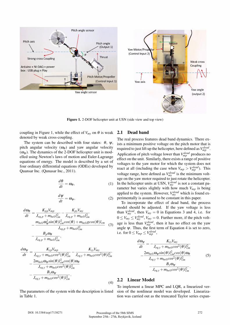
Figure 1. 2-DOF helicopter unit at USN (side view and top view)

coupling in Figure 1, while the effect of Vmy on θ is weakdenoted by weak cross-coupling.

The system can be described with four states: θ , ψ ,pitch angular velocity (ωθ ) and yaw angular velocity(ωψ ). The dynamics of the 2-DOF helicopter unit is mod-elled using Newton′s laws of motion and Euler-Lagrangeequations of energy. The model is described by a set offour ordinary differential equations (ODEs) developed byQuansar Inc. (Qunasar Inc., 2011).

dθ

dt= ωθ , (1)

dψ

dt= ωψ , (2)

dωθ

dt=

KppVmp

Jeq,p +mhelil2cm−

KpyVmy

Jeq,p +mhelil2cm

−mheliω

2ψ sin(θ)l2

cmcos(θ)+mheligcos(θ)lcm

Jeq,p +mhelil2cm

−Bpωθ

Jeq,p +mhelil2cm

,

(3)

dωψ

dt=

KypVmp

Jeq,y +mhelicos2(θ)l2cm−

KyyVmy

Jeq,y +mhelicos2(θ)l2cm

−2mheliωψ sin(θ)l2

cmcos(θ)ωθ

Jeq,y +mhelicos2(θ)l2cm

−Byωψ

Jeq,y +mhelicos2(θ)l2cm

.

(4)

The parameters of the system with the description is listedin Table 1.

2.1 Dead bandThe real process features dead band dynamics. There ex-ists a minimum positive voltage on the pitch motor that isrequired to just lift up the helicopter, here defined as V dead

mp .Application of pitch voltage lower than V dead

mp produces noeffect on the unit. Similarly, there exists a range of positivevoltages to the yaw motor for which the system does notreact at all (including the case when Vmp > V dead

mp ). Thisvoltage range, here defined as V dead

my is the minimum volt-age on the yaw motor required to just rotate the helicopter.In the helicopter units at USN, V dead

my is not a constant pa-rameter but varies slightly with how much Vmp is beingapplied to the system. However, V dead

my which is found ex-perimentally is assumed to be constant in this paper.

To incorporate the effect of dead band, the processmodel should be adjusted. If the yaw voltage is lessthan V dead

my , then Vmy = 0 in Equations 3 and 4, i.e. for0≤Vmy ≤V dead

my , Vmy = 0. Further more, if the pitch volt-age is less than V dead

mp , then it has no effect on the yawangle ψ . Thus, the first term of Equation 4 is set to zero,i.e. for 0≤Vmp ≤V dead

mp ,

dωψ

dt=−

KyyVmy

Jeq,y +mhelicos2(θ)l2cm

−2mheliωψ sin(θ)l2

cmcos(θ)ωθ

Jeq,y +mhelicos2(θ)l2cm

−Byωψ

Jeq,y +mhelicos2(θ)l2cm

.

(5)

2.2 Linear ModelTo implement a linear MPC and LQR, a linearized ver-sion of the nonlinear model was developed. Lineariza-tion was carried out as the truncated Taylor series expan-

DOI: 10.3384/ecp17138271 Proceedings of the 58th SIMS September 25th - 27th, Reykjavik, Iceland

272

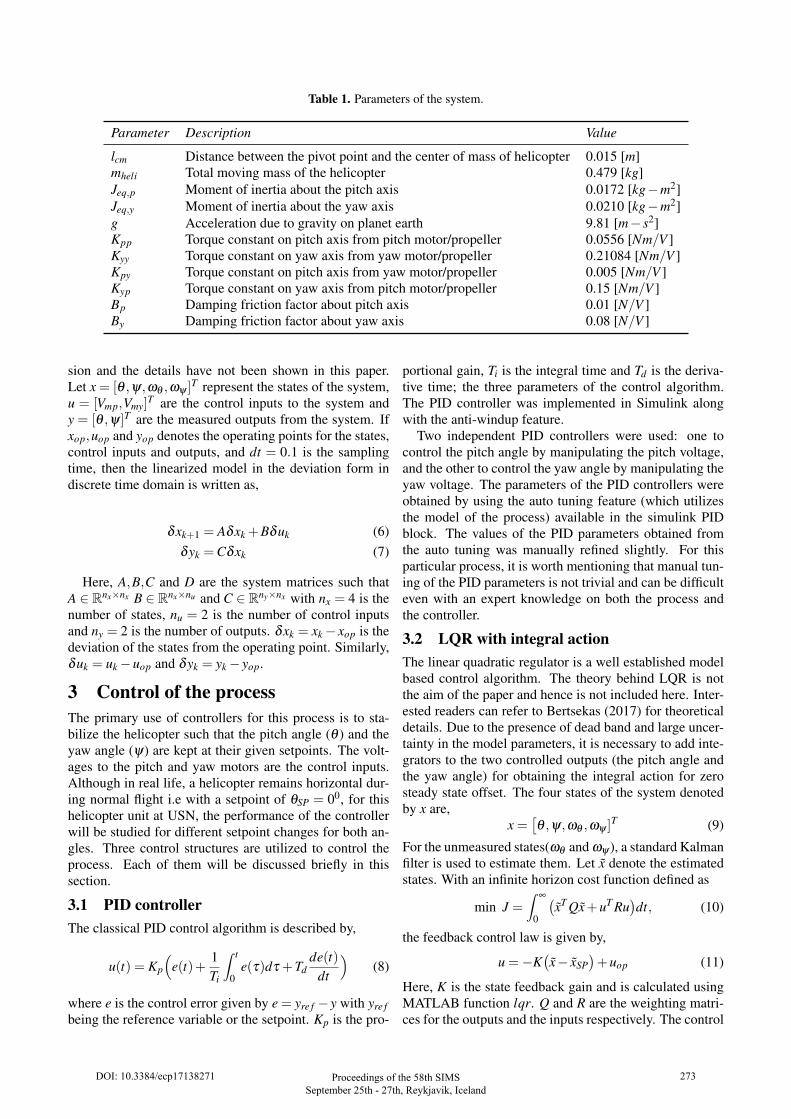
Table 1. Parameters of the system.

Parameter Description Value

lcm Distance between the pivot point and the center of mass of helicopter 0.015 [m]mheli Total moving mass of the helicopter 0.479 [kg]Jeq,p Moment of inertia about the pitch axis 0.0172 [kg−m2]Jeq,y Moment of inertia about the yaw axis 0.0210 [kg−m2]g Acceleration due to gravity on planet earth 9.81 [m− s2]Kpp Torque constant on pitch axis from pitch motor/propeller 0.0556 [Nm/V ]Kyy Torque constant on yaw axis from yaw motor/propeller 0.21084 [Nm/V ]Kpy Torque constant on pitch axis from yaw motor/propeller 0.005 [Nm/V ]Kyp Torque constant on yaw axis from pitch motor/propeller 0.15 [Nm/V ]Bp Damping friction factor about pitch axis 0.01 [N/V ]By Damping friction factor about yaw axis 0.08 [N/V ]

sion and the details have not been shown in this paper.Let x = [θ ,ψ,ωθ ,ωψ ]

T represent the states of the system,u = [Vmp,Vmy]

T are the control inputs to the system andy = [θ ,ψ]T are the measured outputs from the system. Ifxop,uop and yop denotes the operating points for the states,control inputs and outputs, and dt = 0.1 is the samplingtime, then the linearized model in the deviation form indiscrete time domain is written as,

δxk+1 = Aδxk +Bδuk (6)δyk =Cδxk (7)

Here, A,B,C and D are the system matrices such thatA ∈ Rnx×nx B ∈ Rnx×nu and C ∈ Rny×nx with nx = 4 is thenumber of states, nu = 2 is the number of control inputsand ny = 2 is the number of outputs. δxk = xk− xop is thedeviation of the states from the operating point. Similarly,δuk = uk−uop and δyk = yk− yop.

3 Control of the processThe primary use of controllers for this process is to sta-bilize the helicopter such that the pitch angle (θ ) and theyaw angle (ψ) are kept at their given setpoints. The volt-ages to the pitch and yaw motors are the control inputs.Although in real life, a helicopter remains horizontal dur-ing normal flight i.e with a setpoint of θSP = 00, for thishelicopter unit at USN, the performance of the controllerwill be studied for different setpoint changes for both an-gles. Three control structures are utilized to control theprocess. Each of them will be discussed briefly in thissection.

3.1 PID controllerThe classical PID control algorithm is described by,

u(t) = Kp

(e(t)+

1Ti

∫ t

0e(τ)dτ +Td

de(t)dt

)(8)

where e is the control error given by e = yre f −y with yre fbeing the reference variable or the setpoint. Kp is the pro-

portional gain, Ti is the integral time and Td is the deriva-tive time; the three parameters of the control algorithm.The PID controller was implemented in Simulink alongwith the anti-windup feature.

Two independent PID controllers were used: one tocontrol the pitch angle by manipulating the pitch voltage,and the other to control the yaw angle by manipulating theyaw voltage. The parameters of the PID controllers wereobtained by using the auto tuning feature (which utilizesthe model of the process) available in the simulink PIDblock. The values of the PID parameters obtained fromthe auto tuning was manually refined slightly. For thisparticular process, it is worth mentioning that manual tun-ing of the PID parameters is not trivial and can be difficulteven with an expert knowledge on both the process andthe controller.

3.2 LQR with integral actionThe linear quadratic regulator is a well established modelbased control algorithm. The theory behind LQR is notthe aim of the paper and hence is not included here. Inter-ested readers can refer to Bertsekas (2017) for theoreticaldetails. Due to the presence of dead band and large uncer-tainty in the model parameters, it is necessary to add inte-grators to the two controlled outputs (the pitch angle andthe yaw angle) for obtaining the integral action for zerosteady state offset. The four states of the system denotedby x are,

x =[θ ,ψ,ωθ ,ωψ ]

T (9)

For the unmeasured states(ωθ and ωψ ), a standard Kalmanfilter is used to estimate them. Let x denote the estimatedstates. With an infinite horizon cost function defined as

min J =∫

∞

0

(xT Qx+uT Ru

)dt, (10)

the feedback control law is given by,

u =−K(x− xSP

)+uop (11)

Here, K is the state feedback gain and is calculated usingMATLAB function lqr. Q and R are the weighting matri-ces for the outputs and the inputs respectively. The control

DOI: 10.3384/ecp17138271 Proceedings of the 58th SIMS September 25th - 27th, Reykjavik, Iceland

273

signal produced by the output integrators are added to u togenerate the control signal applied to the actual process,

uapp = u+Ki

∫ (y− ySP

)dt (12)

Here, y are the controlled outputs (pitch and yaw angles)with their setpoints ySP and Ki are the output integratorsgain vector. The estimates of the states are obtained as,

δ xk+1 = Aδ xk +Bδuk +L(δyk−δ yk) (13)

xk = δ xk + xop (14)

Here, L is the Kalman filter gain and is calculated usingthe MATLAB function kalman for appropriately chosencovariance matrices for states and measurements.

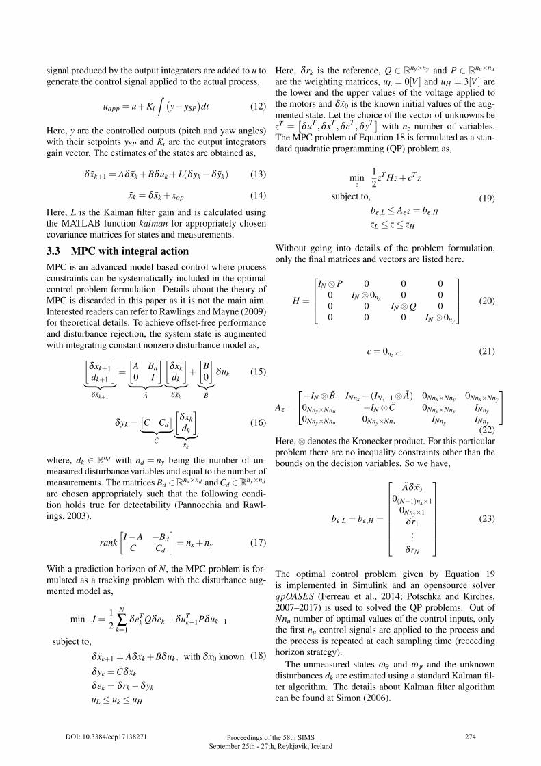
3.3 MPC with integral actionMPC is an advanced model based control where processconstraints can be systematically included in the optimalcontrol problem formulation. Details about the theory ofMPC is discarded in this paper as it is not the main aim.Interested readers can refer to Rawlings and Mayne (2009)for theoretical details. To achieve offset-free performanceand disturbance rejection, the system state is augmentedwith integrating constant nonzero disturbance model as,[

δxk+1dk+1

]︸ ︷︷ ︸

δ xk+1

=

[A Bd0 I

]︸ ︷︷ ︸

A

[δxkdk

]︸ ︷︷ ︸

δ xk

+

[B0

]︸︷︷︸

B

δuk (15)

δyk =[C Cd

]︸ ︷︷ ︸C

[δxkdk

]︸ ︷︷ ︸

xk

(16)

where, dk ∈ Rnd with nd = ny being the number of un-measured disturbance variables and equal to the number ofmeasurements. The matrices Bd ∈Rnx×nd and Cd ∈Rny×nd

are chosen appropriately such that the following condi-tion holds true for detectability (Pannocchia and Rawl-ings, 2003).

rank[

I−A −BdC Cd

]= nx +ny (17)

With a prediction horizon of N, the MPC problem is for-mulated as a tracking problem with the disturbance aug-mented model as,

min J =12

N

∑k=1

δeTk Qδek +δuT

k−1Pδuk−1

subject to,

δ xk+1 = Aδ xk + Bδuk, with δ x0 known

δyk = Cδ xk

δek = δ rk−δyk

uL ≤ uk ≤ uH

(18)

Here, δ rk is the reference, Q ∈ Rny×ny and P ∈ Rnu×nu

are the weighting matrices, uL = 0[V ] and uH = 3[V ] arethe lower and the upper values of the voltage applied tothe motors and δ x0 is the known initial values of the aug-mented state. Let the choice of the vector of unknowns bezT =

[δuT ,δxT ,δeT ,δyT ] with nz number of variables.

The MPC problem of Equation 18 is formulated as a stan-dard quadratic programming (QP) problem as,

minz

12

zT Hz+ cT z

subject to,bε,L ≤ Aε z = bε,H

zL ≤ z≤ zH

(19)

Without going into details of the problem formulation,only the final matrices and vectors are listed here.

H =

IN⊗P 0 0 0

0 IN⊗0nx 0 00 0 IN⊗Q 00 0 0 IN⊗0ny

(20)

c = 0nz×1 (21)

Aε =

−IN⊗ B INnx − (IN,−1⊗ A) 0Nnx×Nny 0Nnx×Nny

0Nny×Nnu −IN⊗C 0Nny×Nny INny

0Nny×Nnu 0Nny×Nnx INny INny

(22)

Here,⊗ denotes the Kronecker product. For this particularproblem there are no inequality constraints other than thebounds on the decision variables. So we have,

bε,L = bε,H =

Aδ x00(N−1)nx×1

0Nny×1δ r1

...δ rN

(23)

The optimal control problem given by Equation 19is implemented in Simulink and an opensource solverqpOASES (Ferreau et al., 2014; Potschka and Kirches,2007–2017) is used to solved the QP problems. Out ofNnu number of optimal values of the control inputs, onlythe first nu control signals are applied to the process andthe process is repeated at each sampling time (receedinghorizon strategy).

The unmeasured states ωθ and ωψ and the unknowndisturbances dk are estimated using a standard Kalman fil-ter algorithm. The details about Kalman filter algorithmcan be found at Simon (2006).

DOI: 10.3384/ecp17138271 Proceedings of the 58th SIMS September 25th - 27th, Reykjavik, Iceland

274

0 20 40 60 80-40

-20

0

[deg

]

Step changes in with PID controler

: SP : real

0 20 40 60 80

50

100

[deg

] : SP : real

0 20 40 60 80time [s]

0

1

2

Vm

p, V

my [V

]

Control inputs

Vmp

Vmy

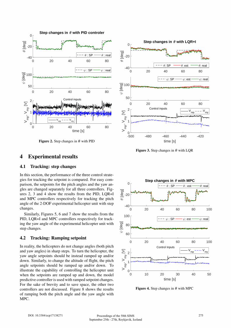
Figure 2. Step changes in θ with PID

4 Experimental results

4.1 Tracking: step changes

In this section, the performance of the three control strate-gies for tracking the setpoint is compared. For easy com-parison, the setpoints for the pitch angles and the yaw an-gles are changed separately for all three controllers. Fig-ures 2, 3 and 4 show the results from the PID, LQR+Iand MPC controllers respectively for tracking the pitchangle of the 2-DOF experimental helicopter unit with stepchanges.

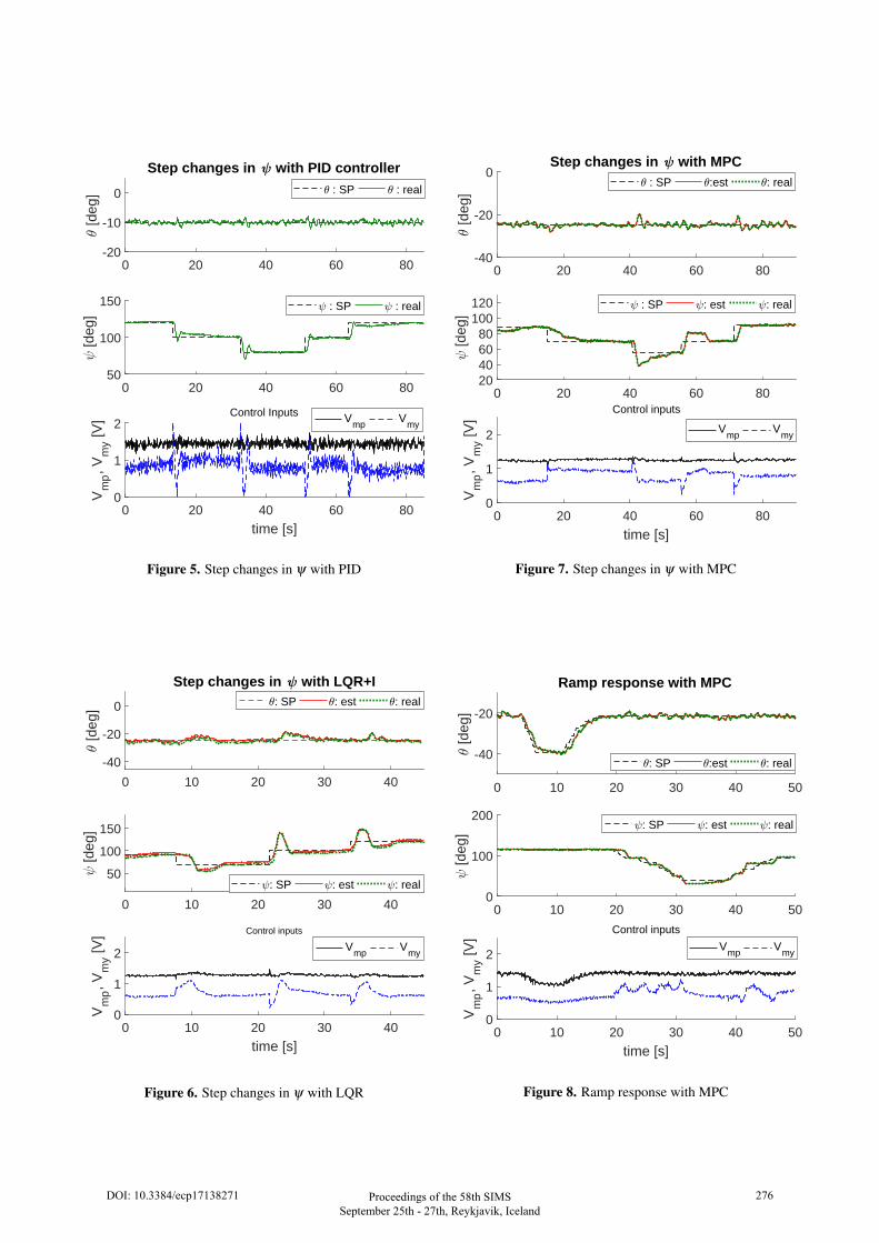
Similarly, Figures 5, 6 and 7 show the results from thePID, LQR+I and MPC controllers respectively for track-ing the yaw angle of the experimental helicopter unit withstep changes.

4.2 Tracking: Ramping setpoint

In reality, the helicopters do not change angles (both pitchand yaw angles) in sharp steps. To turn the helicopter, theyaw angle setpoints should be instead ramped up and/ordown. Similarly, to change the altitude of flight, the pitchangle setpoints should be ramped up and/or down. Toillustrate the capability of controlling the helicopter unitwhen the setpoints are ramped up and down, the modelpredictive controller is used with ramped setpoint changes.For the sake of brevity and to save space, the other twocontrollers are not discussed. Figure 8 shows the resultsof ramping both the pitch angle and the yaw angle withMPC.

0 20 40 60 80-40

-20

0

[deg

]

Step changes in with LQR+I

: SP : est : real

0 20 40 60 80

50

100

[deg

]

: SP : est : real

-500 -480 -460 -440 -420

time [s]

0

1

2

Vm

p, V

my [V

] Control inputsV

mpV

my

Figure 3. Step changes in θ with LQR

0 20 40 60 80 100-40

-20

0

[deg

]

Step changes in with MPC : SP : est : real

0 20 40 60 80 100

60

80

100

[deg

]

: SP : est : real

0 10 20 30 40 50

time [s]

0

1

2

Vm

p, V

my [V

] Control InputsV

mpV

my

Figure 4. Step changes in θ with MPC

DOI: 10.3384/ecp17138271 Proceedings of the 58th SIMS September 25th - 27th, Reykjavik, Iceland

275

0 20 40 60 80-20

-10

0

[deg

]

Step changes in with PID controller : SP : real

0 20 40 60 8050

100

150

[deg

]

: SP : real

0 20 40 60 80

time [s]

0

1

2

Vm

p, V

my [V

] Control Inputs Vmp

Vmy

Figure 5. Step changes in ψ with PID

0 10 20 30 40

-40

-20

0

[deg

]

Step changes in with LQR+I: SP : est : real

0 10 20 30 40

50

100

150

[deg

]

: SP : est : real

0 10 20 30 40

time [s]

0

1

2

Vm

p, V

my [V

] Control inputs

Vmp

Vmy

Figure 6. Step changes in ψ with LQR

0 20 40 60 80-40

-20

0

[deg

]

Step changes in with MPC : SP :est : real

0 20 40 60 8020406080

100120

[deg

]

: SP : est : real

0 20 40 60 80

time [s]

0

1

2

Vm

p, V

my [V

]

Control inputs

Vmp

Vmy

Figure 7. Step changes in ψ with MPC

0 10 20 30 40 50

-40

-20

[deg

]

Ramp response with MPC

: SP :est : real

0 10 20 30 40 500

100

200

[deg

]

: SP : est : real

0 10 20 30 40 50

time [s]

0

1

2

Vm

p, V

my [V

]

Control inputs

Vmp

Vmy

Figure 8. Ramp response with MPC

DOI: 10.3384/ecp17138271 Proceedings of the 58th SIMS September 25th - 27th, Reykjavik, Iceland

276

0 20 40 60 80-50

0

50

[deg

]

Disturbance rejection with PID controller : SP : real

0 20 40 60 8050

100

150

[deg

]

: SP : real

0 20 40 60 80

time [s]

0

1

2

Vm

p, V

my [V

]

Control inputsV

mpV

my

Disturbances

Disturbances

Figure 9. Disturbance rejection with PID

4.3 Disturbance rejectionIn real case scenarios, several disturbances can influencethe flight path of a helicopter. A strong gust of wind, sud-den drop in air pressure and density can all affect the pitchand the yaw angle of the helicopter. Such disturbancesshould be compensated by the controllers in order to sta-bilize the system. For the helicopter prototype at USN, tosupply an external disturbance, the body of the helicopterwas moved by applying force manually by hand. In otherwords, to mimic the presence of disturbance, external per-turbation on the pitch and yaw angles were provided man-ually by the user. Figures 9, 10 and 11 show the perfor-mance of PID, LQR+I and MPC controller respectivelyunder the presence of disturbances.

5 Discussion5.1 Tracking performanceAll the three control strategies could satisfactorily stabi-lize the system for different setpoint changes of both thepitch and the yaw angles. With the PID controller, thederivative term (D) is utmost important and should be usedfor stabilizing the system. A pure proportional and inte-gral (PI) controller was not able to stabilize the system.However, the inclusion of D term was strongly influencedby the measurement noises and the resulting control in-puts became noisy. There was chattering of the voltagesapplied to the motors. In the experimental helicopter unit,the chattering of the voltages resulted in unpleasant vibra-tional sounds from the propellers and mechanical vibra-

0 20 40 60 80

-40

-20

0

20

[deg

]

Disturbance rejection with LQR+I: SP : est : real

0 20 40 60 80

50

100

150

[deg

]

: SP : est : real

-100 -80 -60 -40 -20

time [s]

0

1

2

Vm

p, V

my [V

]

Control inputsV

mpV

my

Disturbance

Disturbance

Figure 10. Disturbance rejection with LQR

0 20 40 60 80 100

-40

-20

0

[deg

]

Disturbance rejection with MPC : SP :est : real

0 20 40 60 80 10050

100

150

[deg

]

: SP : est : real

0 20 40 60 80 100

time [s]

0

1

2

Vm

p, V

my [V

]

Control inputsV

mpV

my

Disturbances

Disturbances

Figure 11. Disturbance rejection with MPC

DOI: 10.3384/ecp17138271 Proceedings of the 58th SIMS September 25th - 27th, Reykjavik, Iceland

277

tions of the whole rotor propeller system. On the otherhand, the model based controllers (LQR+I and MPC) pro-duced relatively cleaner control inputs without any chat-tering. In addition, proper tuning of the PID controllerswas not straight forward owing to the cross coupling na-ture of the process. It is highly recommended that themodel of the process should be used for tuning of the PIDcontrollers. In contrast, it was relatively easier to tune themodel based controllers.

When the setpoints on the pitch angles (yaw angles)were changed, all the three controllers could achieve thenew setpoints while at the same time keeping hold or with-out losing control of the yaw angles (pitch angles), despitethe presence of a strong cross coupling effect between theinputs and the outputs.

As has also been described before, in real life the pitchangle and the yaw angles are not changed in steps but areinstead ramped. The model predictive controller showeda good response to the ramped setpoints. One benefit oframping the helicopter angles is that the control inputs(voltages to the motors) are not suddenly changed by alarge amount but instead they are changed gradually. Thisin practice may/will generate smoother response.

5.2 Disturbance rejection performanceDisturbances were applied manually by the user. Big dis-turbances (more than ±500 deviations) were applied toboth the pitch and the yaw angles. All three controllersshowed relatively equal and satisfactory performance incompensating the disturbances.

5.3 Comments on state estimationThe presence of dead band and the mismatch between themathematical model and the real process makes it inter-esting for state estimation. A standard Kalman filter wasapplied to estimate the unmeasured states and the distur-bances for the model based controllers (LQR+I) and MPC.In Figures 3, 6 and 10 (for the LQR+I controller), it canbe seen that there is a small offset between the estimatedangles (θ : est and ψ : est) and the angles measured bythe sensors (θ : real and ψ : real). However, in Figures4, 7 and 11 (for the MPC controller), it can be seen thatthere is no offset between the estimated angles (θ : est andψ : est) and the angles measured by the sensors (θ : realand ψ : real).

With the MPC, the system states are augmented by adisturbance model (see Equation 15) and the disturbancesare estimated using a Kalman filter. The estimated dis-turbances accounts for the dead band and the model mis-match and hence compensates for any offsets, thus pro-ducing zero offset between the estimated and the mea-sured values. On the other hand, with the LQR+I con-troller, the system states are not augmented with any kindof disturbance model. The presence of dead band andmodel mismatch are hence not compensated, thus produc-ing small offset between the estimated and the measuredvalues. This clearly indicates the fact that due to model

mismatch, such offset can be expected as an output froma Kalman filter algorithm. The important thing is to judgewhether such offsets are important for the control/estima-tion purpose at hand. If they are not important, and theclosed loop response is stable and correct, such offsetsmay simply be discarded.

6 ConclusionThis paper has shown experimental results obtained fromapplying different control structures to a real process. Thecontrol structures used in this paper are standard algo-rithms. They are relatively easier to understand and toimplement. To solve the QP optimal control problems,open source solver which supports code generation is cho-sen. This allows us to implement the model based controlstructures to a real process using Simulink. The built-inQP solvers in MATLAB/Simulink does not support codegeneration and hence cannot be used for real time con-trol of processes with fast dynamics such as the helicopterunit.

For this particular process at USN, the classical PIDcontrollers show relatively as good performance as the ad-vanced model based control structures. However, the con-trol inputs generated by PIDs are noisy. Chattered inputsignals applied to the motor cause vibrations and can in-duce mechanical damage to the unit with time. In addi-tion, model based control such as the MPC has the addedadvantage of including process constraints directly intothe optimization problem. With the PID and LQR+I, con-straints on the inputs were implemented as ad-hoc if-elseconditions. Finally, the paper also justifies that such ex-perimental units can be built from the scratch and can beused for pedagogic purpose with both the classical and theadvanced control algorithms.

ReferencesFernando S. Barbosa, Gabriel P. das Neves, and Bruno A.

Angélico. Discrete lqg/ltr control augmented by inte-grators applied to a 2-dof helicopter. In 2016 IEEEConference on Control Applications (CCA), Sept 2016.doi:10.1109/CCA.2016.7587976.

Dimitri P. Bertsekas. Dynamic Programming and Optimal Con-trol, volume 1. Athena Scientific, fourth edition, 2017. ISBN1-886529-26-4.

Hans Joachim Ferreau, Christian Kirches, Andreas Potschka,Hans Georg Bock, and Moritz Diehl. qpOASES: A paramet-ric active-set algorithm for quadratic programming. Mathe-matical Programming Computation, 6(4):327–363, 2014.

M. Lopez-Martinez, J.M. Diaz, M.G. Ortega, and F.R. Rubio.Control of a laboratory helicopter using switched 2-step feed-back linearization. In Proceedings of the 2004 American Con-trol Conference, volume 5, pages 4330–4335, June 2004.

Jose Guillermo Guarnizo M., Cesar Leonardo Trujillo, andJavier Antonio Guacaneme M. Modeling and control of atwo dof helicopter using a robust control design based on dk

DOI: 10.3384/ecp17138271 Proceedings of the 58th SIMS September 25th - 27th, Reykjavik, Iceland

278

iteration. In IECON 2010 - 36th Annual Conference on IEEEIndustrial Electronics Society, pages 162–167, Nov 2010.doi:10.1109/IECON.2010.5675183.

Giovanni Gallon Neto, Fernando dos Santos Barbosa, andBruno Augusto Angélico. 2-dof helicopter controlling bypole-placements. In 2016 12th IEEE International Confer-ence on Industry Applications (INDUSCON), pages 1–5, Nov2016. doi:10.1109/INDUSCON.2016.7874535.

Gabriele Pannocchia and James B. Rawlings. Disturbance mod-els for offset-free model-predictive control. AIChE Journal,49(2):426–437, 2003.

Hans Joachim Ferreauand Andreas Potschka and ChristianKirches. qpOASES webpage. http://www.qpOASES.org/,2007–2017.

Qunasar Inc. 2-DOF helicopter: Reference Manual, 2011.

James B. Rawlings and David Q. Mayne. Model Predictive Con-trol Theory and Design. Nob Hill Publishing, LLC, 2009.ISBN 978-0-9759377-0-9.

Dan Simon. Optimal state estimation. John Wiley & Sons, Inc.,Hoboken, New Jersey, 2006. ISBN 10 0-471-70858-5.

Juhng-Perng Su, Chi-Ying Liang, and Hung-Ming Chen. Ro-bust control of a class of nonlinear systems and its ap-plication to a twin rotor mimo system. In IndustrialTechnology, 2002. IEEE ICIT ’02. 2002 IEEE Interna-tional Conference, volume 2, pages 1272–1277, Dec 2002.doi:10.1109/ICIT.2002.1189359.

Gwo-Ruey Yu. Robust-optimal control of a nonlineartwo degree-of-freedom helicopter. In 6th IEEE/ACISInternational Conference on Computer and Informa-tion Science (ICIS 2007), pages 744–749, July 2007.doi:10.1109/ICIS.2007.160.

DOI: 10.3384/ecp17138271 Proceedings of the 58th SIMS September 25th - 27th, Reykjavik, Iceland

279