Embed Size (px)
Citation preview
DEVELOPMENT OF A 6 DOF NONLINEAR HELICOPTERMODEL FOR THE MPI CYBERMOTION SIMULATOR
Carlo A. Gerboni, 1,2 Stefano Geluardi, 1,2 Mario Olivari, 1,2 Frank M. Nieuwenhuizen, 1Heinrich H. Bulthoff, 1 and Lorenzo Pollini 2
1Max Planck Institute for Biological CyberneticsSpemannstrasse 38, 72076 Tubingen
Germany2University of Pisa
Via Diotisalvi 2, 56122 PisaItaly
Email: carlo.gerboni; stefano.geluardi; [email protected]; [email protected]
Abstract
This paper describes the different phases of realizing and validating a helicopter model for the MPI CyberMotionSimulator (CMS). The considered helicopter is a UH-60 Black Hawk. The helicopter model was developedbased on equations and parameters available in literature. First, the validity of the model was assessed byperforming tests based on ADS-33E-PRF criteria using closed loop controllers and with a non-expert pilot.Results on simulated data were similar to results obtained with the real helicopter. Second, the validity of themodel was assessed with a helicopter pilot in-the-loop in both a fixed-base simulator and the CMS. The pilotperformed a vertical remask maneuver defined in ADS-33E-PRF. Most metrics for performance were reachedadequately with both simulators. The motion cues in the CMS allowed for improvements in some of the metrics.The pilot was also asked to give a subjective evaluation of the model by answering the Israel Aircraft IndustriesPilot Rating Scale (IAI PRS). Similarly to results of ADS-33E-PRF, pilot responses confirmed that the motioncues provided more realistic flight experience.
NOTATION
a0 main rotor blade lift curve slope (1/rad)
s rotor solidity (-)
u, v, w translational velocity components ofhelicopter along fuselage x-,y-,z-axes(m/s)
p, q, r angular velocity components of he-licopter along fuselage x-,y-,z-axes(rad/s)
pw, qw, rw angular velocity components of heli-copter in hub axes (rad/s). With a barthey are normalized by Ω
k1, k2, k3, k4 augmentation system parameters (-)
CT rotor thrust coefficient (-)
Ixx, Iyy, Izz moments of inertia of the helicopterabout the x-,y-,z-axes (kg m2)
Ma helicopter mass (kg)
R main rotor radius (m)
SE area of the empennage components(fin or tail plane) or of the fuselage (m2)
T main rotor thrust (N )
V forward velocity (m/s)
VE total velocity incident on empennagecomponents (on fin or on tail plane) oron fuselage (m/s)
θ, φ, ψ Euler angles defining the orientation ofthe aircraft relative to the Earth (rad)
β0, β1c, β1s rotor blade coning, longitudinal and lat-eral flapping angles (rad)
β1cw, β1sw longitudinal and lateral pitch angle inhub axes (rad)
λ0, λ1c, λ1s rotor uniform and first harmonic inflowvelocities (normalized by ΩR)
θ0 collective pitch angle (rad)
θ1c, θ1s lateral and longitudinal pitch angle(rad)
θ1cw, θ1sw lateral and longitudinal pitch angle inhub axes (rad)
θ0T tail rotor collective pitch angle (rad)
θtw main rotor blade linear twist (rad)
η0, η1c, η1s collective lever and cyclic stick posi-tion (normalized by the stick deflectionrange)
γ Lock number (−)
ρ air density (kg/m3)
µ advance ratio (V/(ΩR))
µz velocity of the rotor hub in hub/shaftaxes (normalized by ΩR)
Ω main rotor speed (rad/s)
1. INTRODUCTION
An investigation on how to make a Personal Air Ve-hicle (PAV) as easy to fly as driving a car is currentlyconducted at the Max Planck Institute for BiologicalCybernetics, under the myCopter EU funded researchprogram.[1] In these studies, rotorcraft vehicles areconsidered as the main reference since their dynam-ics and kinematics best reflect those of a PAV. A key
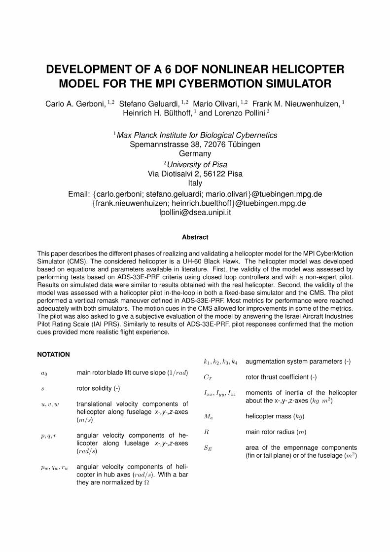
facility that is essential for these studies is the MPI’sCybermotion Simulator (CMS) shown in Figure 1. TheCMS is an anthropomorphic robot with eight degreesof freedom and a cabin as end-effector capable ofhosting a person. The cabin is equipped with a stereoprojection system. A 10 meters linear track allows toincrease the workspace of the robot. Different vehicledynamics models can be simulated in its large motionenvelope.
So far, experiments related to helicopter models werealready performed on the CMS but only with simplifieddynamics.[2] However, recent studies at the MPI ledto considering implementing a more complex and re-alistic helicopter model. These studies consist of thedevelopment of new human-machine interface tech-nologies, [3] investigation of pilots behavior, training ofnon-expert pilots, implementation of new control sys-tems to be tested in simulation with human in-the-loopand training of pilots for performing specific maneu-vers for system identification purposes.[4] Therefore,it was decided to implement a full-flight nonlinear dy-namic helicopter model to be used in the CMS.
Figure 1: The 8 DoF MPI CyberMotion Simulator(http://www.cyberneum.de/).
Nonlinear models for unmanned small-size he-licopters have been investigated and tested inliterature.[5] On the contrary, nonlinear models for full-size helicopters are not very common, due to the diffi-culty of accurately implementing the components ofthe vehicle and obtaining reliable aerodynamic pa-rameters. Few nonlinear helicopter models have beendeveloped and tested in motion simulators but theyare not readily available.[6, 7]
This paper presents the main steps considered for de-veloping a mathematical helicopter model for use inthe CMS. The complexity of the implemented modeland the large motion envelope of the simulator shouldallow for simulating highly realistic flight scenarios. Asfirst step, the model was implemented and validatedby performing several test maneuvers with the help ofclosed-loop controllers. After that, a helicopter pilot
was asked to evaluate the model in a fixed-base sim-ulator. Finally, the same pilot evaluated the model inthe CMS.
The paper is organized as follows: Section 2 de-scribes the development of the model. Section 3presents the results of the time and frequency domainanalysis done on the model. Section 4 is dedicated tothe experiments with the helicopter pilot in the fixed-base simulator and in the CMS. Finally, future stepsare summarized.
2. MODEL DEVELOPMENT
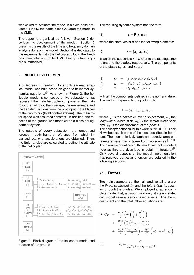
A 6 Degrees of Freedom (DoF) nonlinear mathemat-ical model was built based on generic helicopter dy-namics equations.[8] As shown in Figure 2, the he-licopter model is composed of five subsystems thatrepresent the main helicopter components: the mainrotor, the tail rotor, the fuselage, the empennage andthe transfer functions from the pilot input to the bladesof the two rotors (flight control system). The main ro-tor speed was assumed constant. In addition, the re-action of the ground was modeled as a mass-spring-damper system.
The outputs of every subsystem are forces andtorques in body frame of reference, from which lin-ear and rotational accelerations are obtained. Then,the Euler angles are calculated to define the attitudeof the helicopter.
u = −(wq − qr) + XMa
− gsin(θ)
v = −(ur − wp) + YMa
+ gcos(θ)sin(φ)
w = −(vp− uq) + ZMa
− gcos(θ)cos(φ)
MAIN
ROTOR
TAIL
ROTOR
FUSELAGE
X = XMR +XF +XGR
Y = YMR + YTR + YF + YFN + YGR
Z = ZMR + ZF + ZTP + ZGR
M =MMR +MF +MTP +MGR
L = LMR + LTR + LFN + LGR
N = NMR +NTR +NF +NFN +NGR
Ixxp = (Iyy − Izz)qr + Ixz(r + pq) + L
Iyy q = (Izz − Ixx)rp+ Ixz(r2 − p2) +M
Izz r = (Ixx − Iyy)pq + Ixz(p− qr) +N
(MR)
(TR)
(F )
FIN(FN)
TAIL PLANE(TP )
&
GROUND
REACTION(GR)
EULER ANGLES(φ, θ, ψ)
FLIGHT CONTROL SYSTEM
Figure 2: Block diagram of the helicopter model andreaction of the ground
The resulting dynamic system has the form
x = Fx,u, t(1)
where the state vector x has the following elements:
x = xf ,xr,xb(2)
in which the subscripts f, r, b refer to the fuselage, therotors and the blades, respectively. The componentsof the states xf , xr and xc are:
xf = u, v, w, p, q, r, φ, θ, ψ(3)xr = β0, β1c, β1s, λ0, λ1c, λ1s(4)xc = θ0, θ1c, θ1s, θ0T (5)
with all the components defined in the nomenclature.The vector u represents the pilot inputs:
u = η0, η1s, η1c, η0T (6)
where η0 is the collective lever displacement, η1s thelongitudinal cyclic stick, η1c is the lateral cyclic stickand η0T is the displacement of the pedals.The helicopter chosen for this work is the UH-60 BlackHawk because it is one of the most described in litera-ture. The mechanical, dynamic and aerodynamic pa-rameters were mainly taken from two sources.[9, 10]
The dynamic equations of the model are not repeatedhere as they are described in detail in literature.[8]
Only several aspects of the model implementationthat received particular attention are detailed in thefollowing sections.
2.1. Rotors
Two main parameters of the main and the tail rotor arethe thrust coefficient CT and the total inflow λ0 pass-ing through the blades. We employed a rather com-plete model that, although valid only at steady state,can model several aerodynamic effects. The thrustcoefficient and the total inflow equations are:
CT =a0s
2
(θ0
(1
3+µ2
2
))(7)
+a0s
2
(µ2
(θ1sw +
pw2
))+
a0s
2
(µz − λ0
2
)+a0s
2
(1
4(1 + µ2)θtw
)
λ0 =CT
2√
[µ2 + (λ0 − µz)2](8)
The two parametersCT and λ0 depend on each other;this makes computing the flight condition complex.Different approaches have been proposed to calcu-late the solution of equations 7 and 8. For instance,a closed-form solution for CT and λ0 can be foundfor each specific flight condition (take off, hover, for-ward flight and landing).[8] However, this approachimplies switching between different sets of equationswhen simulating the model in different steady states.Hence, an iterative solution based on a Newton-Rhapson method was applied to arrive at a model thatis valid in all flight conditions.Another issue we encountered during the develop-ment was the relation between the blade pitch anglesand the displacement of the swashplate. Differentmodels [8, 12, 13] were tested in order to find the re-lationship that better approximate the response of thereal helicopter.[14] Best accuracy was obtained with amethod that reduce much the effect of the blade lin-ear twist θtw, that in helicopter like the UH-60 has animportant influence due to its big value:[13]
β0 = γ
[θ08
(1 + µ2) +θtw10
(1 +5
6µ2) +
µ
6θ1sw −
λ06
](9)
β1sw = θ1cw +(− 4
3µβ0)
(1 + 12µ
2)(10)
β1cw = −θ1sw+− 8
3µ[θ0 − 34λ0 + 3
4µθ1sw + 34θtw]
1− 12µ
2(11)
2.2. Aerodynamics of fuselage and em-pennage
Aerodynamic equations for fuselage and empennagegenerally change between different steady states anddifferent helicopters. Data from wind tunnel tests ineach steady state are necessary for describing theevolution of these equations. Our approach consistedof implementing generic equations that could also beused for other helicopters than the UH-60 consideredin this paper. The generic equations for drag is givenas:
1
2ρV 2
ESECEfriction(E ∈ fin, tailplane, fuselage)
(12)
The friction coefficient CEfrictionis defined differently
for the fuselage and for the empennage. For the fuse-lage it is derived from table look-up functions madewith generalized aerodynamic coefficients.[8] For theempennage it is defined as
CEfriction=
ksin(α) : |Cfriction| < δ−δ ∗ sgn(sin(α)) : |Cfriction| > δ
(13)
in which α is the angle of incidence of the air with thetail plane and with the fin. In this model, the limit factorδ and the scaling factor k are taken by approximatedwind tunnel equations of the empennage.[9, 10] Thiswas done for this helicopter because a detailed reportis present in literature.[10] However, these variablescan also be tuned manually or with the help of an ex-perienced pilot.
2.3. Stability Augmentation System
The model input vector is composed of the four con-trols (collective, lateral and longitudinal cyclic andpedals). The pilot changes the blade pitch describedin (5) by moving the controls.
The UH-60 features a Stability Augmentation System(SAS) that is used to aid the pilot. We only consid-ered such a system for the cyclic controls, as theseare considered most difficult to use. The transfer func-tions that connect the cyclic input of the pilot with themain rotor blade pitch are
θ1c =(a1η1c + b1) + k1p+ k2φ
1 + τs(14)
θ1s =(a2η1s + b2) + k3 q + k4θ
1 + τs(15)
In which (a1, a2) and (b1, b2) define the angular rangesfor θ1c and θ1s. (k1, k2, k3, k4) are the parameters ofthe SAS. The SAS parameters are tuned to obtainfrequency responses similar to the real helicopter asit was active during all the tests.[15] At the same timethe contribution of the SAS is saturated in such a waythat physical limits of the blades are not exceeded.
3. VALIDATION WITH CLOSED-LOOP CON-TROLLERS
This section presents validation tests performed withclosed-loop controllers such that the tests can beperformed without an experienced pilot. Differentanalyses were performed that cover different aspectsof a helicopter model. Two tests will be presentedthat were performed in the time and frequencydomain. The results were compared with flight testdata from literature. All simulations were done withMATLAB/Simulink and a basic virtual environment
developed in Unity3D.
By definition the Aeronautical Design Standard (ADS-33E-PRF) defines the desired Handling Qualities formilitary helicopters.[16] The ADS-33E-PRF tests canbe divided in two groups: quantitative tests and MTEs(Mission Task Elements). The quantitative tests re-quires giving a specific input (i.e. steps and sweepingsinusoids) and evaluating the responses of the rotor-craft in the time and frequency domain. MTEs arecomposed of specific maneuvers that a pilot needs toaccomplish while respecting some performance met-rics. This section describes the quantitative testswhile the MTEs are detailed in Section 4.
3.1. Helicopter in hover with controllers
To control the helicopter in hover condition, controllerswere designed as Proportional, Integral, Derivative(PID) regulators. These controllers regulated the ac-tual speed of the rotorcraft to a reference value bycontrolling the blade pitch angles. For the hover con-dition, all the reference velocities were set to zero.Table 1 presents the blade pitch of the model com-pared with results from flight tests.[14] The compar-ison shows that the collective and the longitudinalpitch are almost the same while the lateral pitch hasa little difference. From this first simulation, it wasshown that trimming the model in hover resulted insimilar responses of the blades compared to a flighttest.
Table 1: Blade pitch angles in hover (angles are givenin degrees)
Flight test[14] Modelθ0 ' 8 ' 8θ1c ' 3.5 ' 1.5θ1s ' −3.5 ' −3
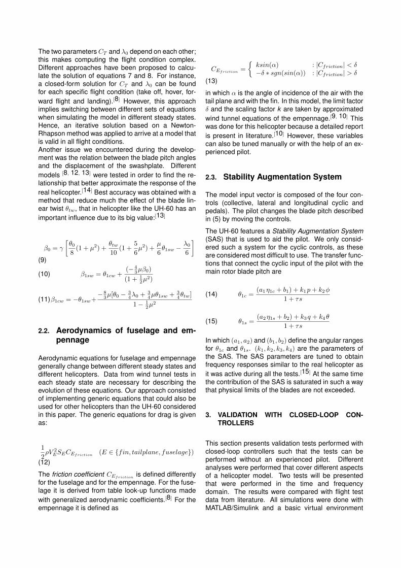
3.2. Attitude quickness test
The first quantitative test is the attitude quickness re-sponse. The aim of this test is to study the quicknessof the rotorcraft at changing its attitude in response toa step input. The evaluated metrics are
roll attitude quickness =ppk∆φ
(16)
pitch attitude quickness =qpk∆θ
(17)
The parameters ppk, qpk,∆φ and ∆θ are highlighted inFigure 3.
5 6 7 8 9 100.4
0.5
0.6
0.7
0.8
0.9
Lat.stickposition(-)
5 6 7 8 9 10−20
0
20
40
Rollrate
(deg/sec)
↑|
ppk|↓
5 6 7 8 9 10−10
0
10
20
30
Time (sec)
Rollattitude(deg)
↑|
∆φpk|↓
↑∆φmin
|↓
Figure 3: Lateral cyclic input for roll attitude quick-ness. Parameters involved in the test are highlighted.The range of the cyclic stick is between 0 and 1
To compare results of our model with those obtainedwith a real helicopter, we replicated the same pilot in-put [15] with a joystick to have a left and right roll,and a forward and backward pitch while controllingthe other axes in hover with the PID controllers. Thesmall duration of the input and the use of the PID con-trollers for the other axes allowed performing this taskwithout an experienced pilot.
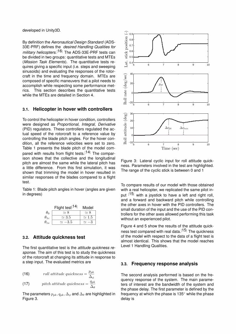
Figure 4 and 5 show the results of the attitude quick-ness test compared with real data.[15] The quicknessof the model with respect to the data of a flight test isalmost identical. This shows that the model reachesLevel 1 Handling Qualities.
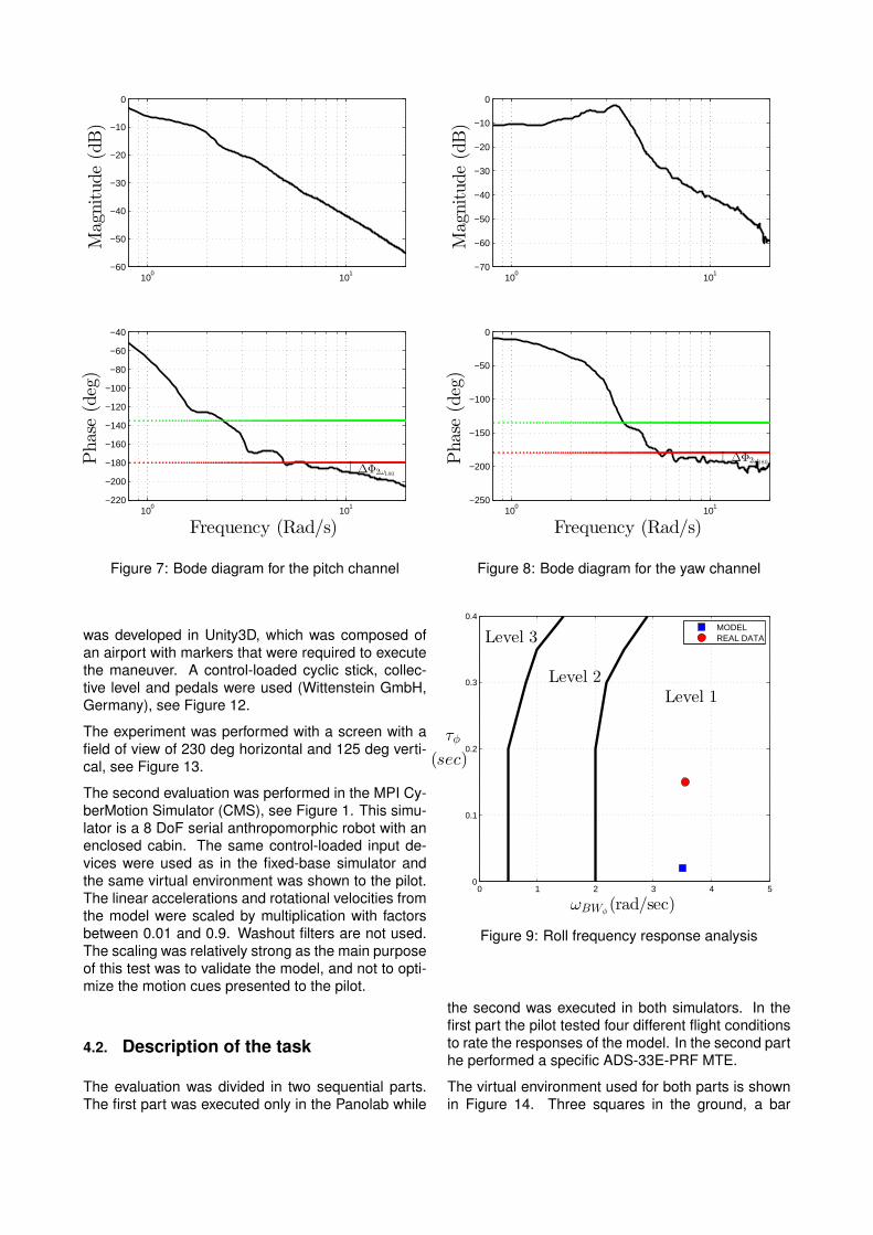
3.3. Frequency response analysis
The second analysis performed is based on the fre-quency response of the system. The main parame-ters of interest are the bandwidth of the system andthe phase delay. The first parameter is defined by thefrequency at which the phase is 135 while the phasedelay is
0 10 20 30 40 50 600
0.5
1
1.5
2
2.5
∆φmin(deg)
ppk∆φpk
(1/sec)
Level 3
Level 2
Level 1
MODEL rightMODEL leftREAL DATA rightREAL DATA left
Figure 4: Roll attitude quickness test
0 10 20 30 40 50 600
0.5
1
1.5
2
2.5
∆θmin(deg)
qpk∆θpk
(1/sec)
Level 2
Level 1
MODEL upMODEL downREAL DATA upREAL DATA down
Figure 5: Pitch attitude quickness test
τp =∆Φ2ω180
57.3× 2ω180(18)
in which 2ω180 indicates two times the frequency atwhich the phase is 180 while ∆Φ2ω180
is the phasedifference between ω180 and 2ω180.[8] At the MaxPlanck Institute for Biological Cybernetics studies ofrotorcraft identification are conducted [17] based ona method developed in literature.[18] Using this work,the frequency responses of the model were obtainedfor the roll, pitch and yaw degrees of freedom with thehelicopter in hover. A small amplitude sweeping sinu-soid signal was given as input for the DoF of interestand the corresponding Euler angle was considered asoutput. The Bode diagrams for roll, pitch and yaw areshown in Figure 6, in Figure 7 and in Figure 8, respec-tively and the parameters required for equation 18 arehighlighted.The phase delay results are given in Figures 9, 10and 11. Two different observations can be made from
100
101
−50
−40
−30
−20
−10
0
10
Magnitude(dB)
100
101
−220
−200
−180
−160
−140
−120
−100
−80
−60
−40
∆Φ2ω180
l
Frequency (Rad/s)
Phase(deg)
Figure 6: Bode diagram for the roll channel
the results: the bandwidth of the identified system isalmost the same of the real vehicle for all three chan-nels. However, the roll and pitch responses show adifferent phase delay caused by a smaller ∆Φ2ω180
of the model compared with the real system at highfrequencies. The causes for this effect are currentlyunder investigation.
4. VALIDATION WITH A HELICOPTER PILOT
The tests described in the previous section showedthe similarity of the model with the real helicopter. Inthe second step, the model was tested with a heli-copter pilot. The tests were done in fixed-base sim-ulator and a motion simulator. The same maneuverwas performed in both simulators. The pilot was in-structed maintain the performance levels defined inthe ADS-33E-PRF criteria as best as possible duringthe maneuver task.
4.1. Experimental setups
The first evaluation with the pilot was executed in afixed-base simulator. The simulation was executedwith a real-time pc. A complex virtual environment
100
101
−60
−50
−40
−30
−20
−10
0Magnitude(dB)
100
101
−220
−200
−180
−160
−140
−120
−100
−80
−60
−40
∆Φ2ω180l
Frequency (Rad/s)
Phase(deg)
Figure 7: Bode diagram for the pitch channel
was developed in Unity3D, which was composed ofan airport with markers that were required to executethe maneuver. A control-loaded cyclic stick, collec-tive level and pedals were used (Wittenstein GmbH,Germany), see Figure 12.
The experiment was performed with a screen with afield of view of 230 deg horizontal and 125 deg verti-cal, see Figure 13.
The second evaluation was performed in the MPI Cy-berMotion Simulator (CMS), see Figure 1. This simu-lator is a 8 DoF serial anthropomorphic robot with anenclosed cabin. The same control-loaded input de-vices were used as in the fixed-base simulator andthe same virtual environment was shown to the pilot.The linear accelerations and rotational velocities fromthe model were scaled by multiplication with factorsbetween 0.01 and 0.9. Washout filters are not used.The scaling was relatively strong as the main purposeof this test was to validate the model, and not to opti-mize the motion cues presented to the pilot.
4.2. Description of the task
The evaluation was divided in two sequential parts.The first part was executed only in the Panolab while
100
101
−70
−60
−50
−40
−30
−20
−10
0
Magnitude(dB)
100
101
−250
−200
−150
−100
−50
0
∆Φ2ω180l
Frequency (Rad/s)
Phase(deg)
Figure 8: Bode diagram for the yaw channel
0 1 2 3 4 50
0.1
0.2
0.3
0.4
ωBWφ(rad/sec)
τφ
(sec)
Level 3
Level 2Level 1
MODELREAL DATA
Figure 9: Roll frequency response analysis
the second was executed in both simulators. In thefirst part the pilot tested four different flight conditionsto rate the responses of the model. In the second parthe performed a specific ADS-33E-PRF MTE.
The virtual environment used for both parts is shownin Figure 14. Three squares in the ground, a bar
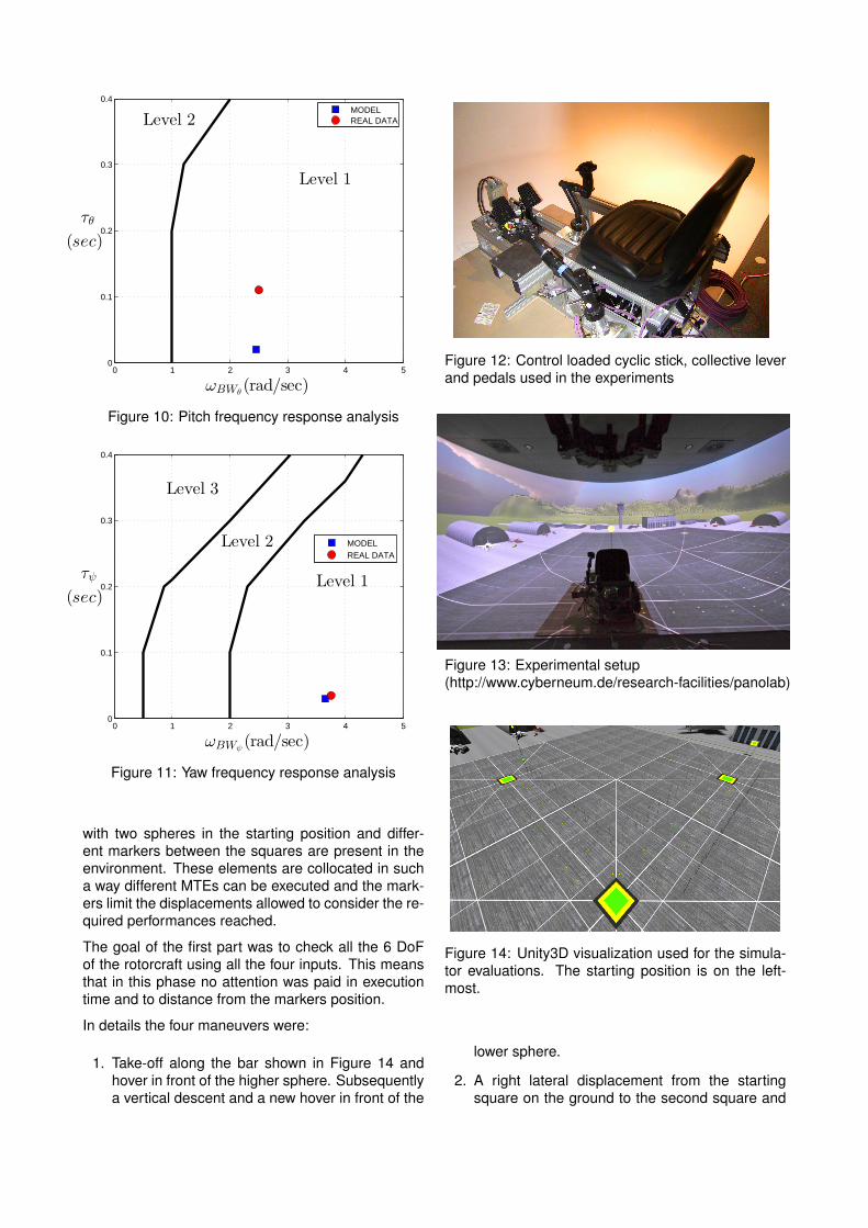
0 1 2 3 4 50
0.1
0.2
0.3
0.4
ωBWθ(rad/sec)
τθ
(sec)
Level 2
Level 1
MODELREAL DATA
Figure 10: Pitch frequency response analysis
0 1 2 3 4 50
0.1
0.2
0.3
0.4
ωBWψ(rad/sec)
τψ
(sec)
Level 3
Level 2
Level 1
MODELREAL DATA
Figure 11: Yaw frequency response analysis
with two spheres in the starting position and differ-ent markers between the squares are present in theenvironment. These elements are collocated in sucha way different MTEs can be executed and the mark-ers limit the displacements allowed to consider the re-quired performances reached.
The goal of the first part was to check all the 6 DoFof the rotorcraft using all the four inputs. This meansthat in this phase no attention was paid in executiontime and to distance from the markers position.
In details the four maneuvers were:
1. Take-off along the bar shown in Figure 14 andhover in front of the higher sphere. Subsequentlya vertical descent and a new hover in front of the
Figure 12: Control loaded cyclic stick, collective leverand pedals used in the experiments
Figure 13: Experimental setup(http://www.cyberneum.de/research-facilities/panolab)
Figure 14: Unity3D visualization used for the simula-tor evaluations. The starting position is on the left-most.
lower sphere.
2. A right lateral displacement from the startingsquare on the ground to the second square and
back again.
3. Forward flight from the second square to the thirdand back again.
4. A 360 turn around the bar.
After each maneuver, the pilot rating scale (PRS) wasused by the pilot to assess the model. This PRSasks the pilot to evaluate the primary response andthe secondary response of each executed maneuver.As an example, for the maneuver 1, the primary re-sponse is given by the use of the collective for thevertical movement, while the secondary response isthe compensatory action that the pilot does with thepedals to counteract the yaw motion. In addition he isasked to rate the difficulties in executing the maneu-ver in relation to the response of the model and withthe visualization.
The second part is the execution of a specificMTE.[16] The maneuver chosen is the vertical re-mask. This maneuver is composed of three parts:
1. The maneuver starts with a vertical remask froma stabilized hover at 75 ft to an altitude of 35 ft(slightly modified from the original maneuver [16])
2. Lateral displacement of 300 ft
3. Stabilize in a new hover position
This maneuver was chosen for several reasons. Firstof all it covers different flight conditions: the initial takeoff to reach the first hover position where the maneu-ver starts, the vertical descent and the fast lateraldisplacement. Second with this maneuver it is pos-sible to use all the inputs of the system: the pedalsare used to counteract turns during the displacement,the lateral cyclic for the lateral displacement, the lon-gitudinal cyclic for maintaining the longitudinal posi-tion and the collective to maintain altitude. Third, withthe lateral displacement is possible to exploit the lin-ear track of the CMS for a more realistic reproductionof lateral accelerations. The markers placed in theenvironment indicate the adequate or desired perfor-mance as defined in ADS-33E-PRF for both condi-tions.
The pilot that performed the test has experience withreal helicopters and with simulators. He has about110 flight hours with around 700 take offs and land-ings. For the simulators he flew a Bell UH-1D in dif-ferent sessions.
4.3. Dependent measures
As the nonlinear dynamic helicopter model describedin this paper is intended to be used to investigate pi-
lots behavior, to record data for system identificationpurposes and to test new control systems to use withhuman in-the-loop, it is necessary to show that themodel can be used to perform complex tasks. There-fore, more attention was given to some of the met-rics as defined in ADS-33E-PRF [16] because theyare independent from possible visualization difficul-ties. These metrics are
1. Maintain altitude after remask and during dis-placement within +10 ft and -15 ft (± 10 ft to bedesired)
2. Maintain heading within ± 15 deg (10 deg to bedesired)
3. Achieve the final stabilized hover within 25 sec ofinitiating the maneuver (15 sec to be desired)
4.4. Results
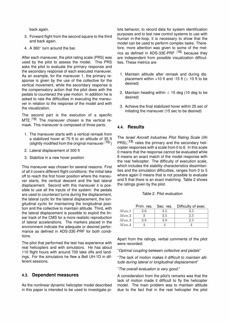
The Israel Aircraft Industries Pilot Rating Scale (IAIPRS),[18] rates the primary and the secondary heli-copter responses with a scale from 0 to 6. In this scale0 means that the response cannot be evaluated while6 means an exact match of the model response withthe real helicopter. The difficulty of execution scale,which includes the stability characteristics dissimilari-ties and the simulation difficulties, ranges from 0 to 5where again 0 means that is not possible to evaluateand 5 that there is an exact matching. Table 2 showsthe ratings given by the pilot.
Table 2: Pilot evaluation
Prim. res. Sec. res. Difficulty of exec.Man.1 3.6 3.5 3.5Man.2 3 3.5 2.5Man.3 3.8 3.8 2.5Man.4 4 4 4
Apart from the ratings, verbal comments of the pilotwere recorded:
”Optimal coupling between collective and pedals”
”The lack of motion makes it difficult to maintain alti-tude during lateral or longitudinal displacement”
”The overall evaluation is very good.”
A consideration from the pilot’s remarks was that thelack of motion made it difficult to fly the helicoptermodel. The main problem was to maintain altitudedue to the fact that in the real helicopter the pilot
”feels” the movement more than he can see the move-ment. So we expected an improvement of the perfor-mance with a motion simulator. Table 3 shows perfor-mances reached for both simulators:
Table 3: Performances in the two simulators
Panolab CMSMetric 1 Adequate DesiredMetric 2 Desired DesiredMetric 3 NotReached NotReached
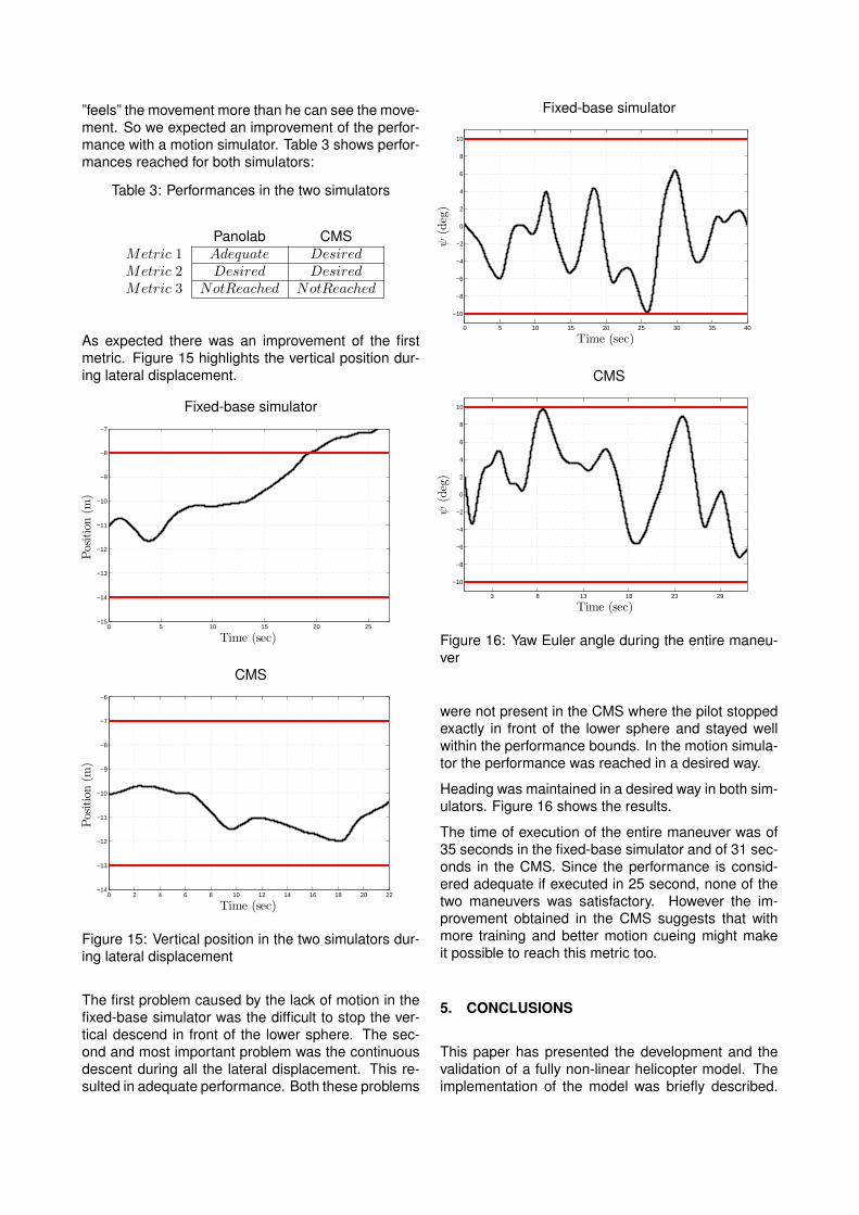
As expected there was an improvement of the firstmetric. Figure 15 highlights the vertical position dur-ing lateral displacement.
Fixed-base simulator
0 5 10 15 20 25−15
−14
−13
−12
−11
−10
−9
−8
−7
Time (sec)
Position(m
)
CMS
0 2 4 6 8 10 12 14 16 18 20 22−14
−13
−12
−11
−10
−9
−8
−7
−6
Time (sec)
Position(m
)
Figure 15: Vertical position in the two simulators dur-ing lateral displacement
The first problem caused by the lack of motion in thefixed-base simulator was the difficult to stop the ver-tical descend in front of the lower sphere. The sec-ond and most important problem was the continuousdescent during all the lateral displacement. This re-sulted in adequate performance. Both these problems
Fixed-base simulator
0 5 10 15 20 25 30 35 40
−10
−8
−6
−4
−2
0
2
4
6
8
10
Time (sec)
ψ(deg)
CMS
3 8 13 18 23 29
−10
−8
−6
−4
−2
0
2
4
6
8
10
Time (sec)
ψ(deg)
Figure 16: Yaw Euler angle during the entire maneu-ver
were not present in the CMS where the pilot stoppedexactly in front of the lower sphere and stayed wellwithin the performance bounds. In the motion simula-tor the performance was reached in a desired way.
Heading was maintained in a desired way in both sim-ulators. Figure 16 shows the results.
The time of execution of the entire maneuver was of35 seconds in the fixed-base simulator and of 31 sec-onds in the CMS. Since the performance is consid-ered adequate if executed in 25 second, none of thetwo maneuvers was satisfactory. However the im-provement obtained in the CMS suggests that withmore training and better motion cueing might makeit possible to reach this metric too.
5. CONCLUSIONS
This paper has presented the development and thevalidation of a fully non-linear helicopter model. Theimplementation of the model was briefly described.
Fixed-base simulator
0 5 10 15 20 25 30 35 40
−20
0
20
40
60
80
100
Time (sec)
Position(m
)
xyz
CMS
0 5 10 15 20 25 30
−20
0
20
40
60
80
100
Time (sec)
Position(m
)
xyz
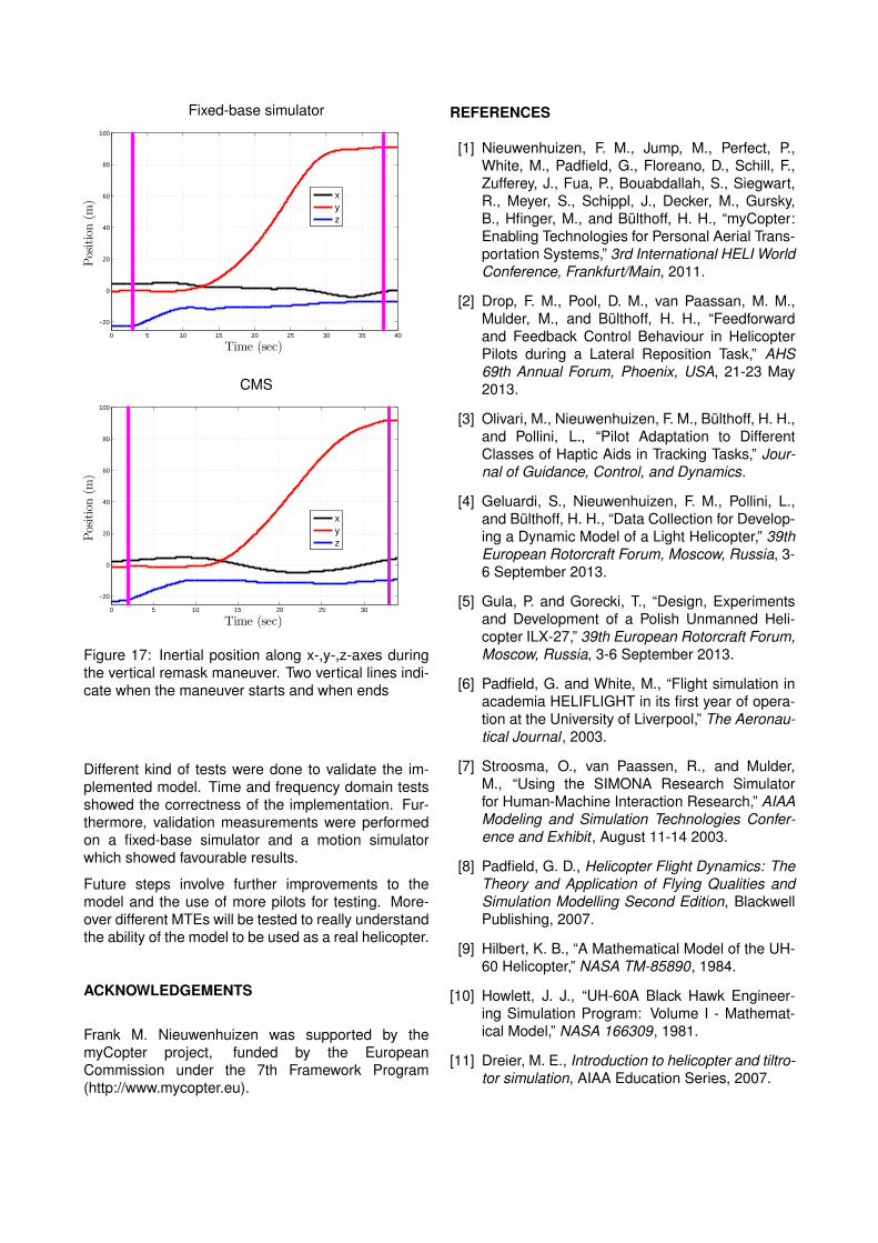
Figure 17: Inertial position along x-,y-,z-axes duringthe vertical remask maneuver. Two vertical lines indi-cate when the maneuver starts and when ends
Different kind of tests were done to validate the im-plemented model. Time and frequency domain testsshowed the correctness of the implementation. Fur-thermore, validation measurements were performedon a fixed-base simulator and a motion simulatorwhich showed favourable results.
Future steps involve further improvements to themodel and the use of more pilots for testing. More-over different MTEs will be tested to really understandthe ability of the model to be used as a real helicopter.
ACKNOWLEDGEMENTS
Frank M. Nieuwenhuizen was supported by themyCopter project, funded by the EuropeanCommission under the 7th Framework Program(http://www.mycopter.eu).
REFERENCES
[1] Nieuwenhuizen, F. M., Jump, M., Perfect, P.,White, M., Padfield, G., Floreano, D., Schill, F.,Zufferey, J., Fua, P., Bouabdallah, S., Siegwart,R., Meyer, S., Schippl, J., Decker, M., Gursky,B., Hfinger, M., and Bulthoff, H. H., “myCopter:Enabling Technologies for Personal Aerial Trans-portation Systems,” 3rd International HELI WorldConference, Frankfurt/Main, 2011.
[2] Drop, F. M., Pool, D. M., van Paassan, M. M.,Mulder, M., and Bulthoff, H. H., “Feedforwardand Feedback Control Behaviour in HelicopterPilots during a Lateral Reposition Task,” AHS69th Annual Forum, Phoenix, USA, 21-23 May2013.
[3] Olivari, M., Nieuwenhuizen, F. M., Bulthoff, H. H.,and Pollini, L., “Pilot Adaptation to DifferentClasses of Haptic Aids in Tracking Tasks,” Jour-nal of Guidance, Control, and Dynamics.
[4] Geluardi, S., Nieuwenhuizen, F. M., Pollini, L.,and Bulthoff, H. H., “Data Collection for Develop-ing a Dynamic Model of a Light Helicopter,” 39thEuropean Rotorcraft Forum, Moscow, Russia, 3-6 September 2013.
[5] Gula, P. and Gorecki, T., “Design, Experimentsand Development of a Polish Unmanned Heli-copter ILX-27,” 39th European Rotorcraft Forum,Moscow, Russia, 3-6 September 2013.
[6] Padfield, G. and White, M., “Flight simulation inacademia HELIFLIGHT in its first year of opera-tion at the University of Liverpool,” The Aeronau-tical Journal , 2003.
[7] Stroosma, O., van Paassen, R., and Mulder,M., “Using the SIMONA Research Simulatorfor Human-Machine Interaction Research,” AIAAModeling and Simulation Technologies Confer-ence and Exhibit , August 11-14 2003.
[8] Padfield, G. D., Helicopter Flight Dynamics: TheTheory and Application of Flying Qualities andSimulation Modelling Second Edition, BlackwellPublishing, 2007.
[9] Hilbert, K. B., “A Mathematical Model of the UH-60 Helicopter,” NASA TM-85890, 1984.
[10] Howlett, J. J., “UH-60A Black Hawk Engineer-ing Simulation Program: Volume I - Mathemat-ical Model,” NASA 166309, 1981.
[11] Dreier, M. E., Introduction to helicopter and tiltro-tor simulation, AIAA Education Series, 2007.
[12] Banks, C., “Lessons on Helicopter dynamic,”(http://www.aerojockey.com/papers/helicopter).
[13] Li, Y., “Principles of Heli-copter Aerodynamic chapter 4,”(http://www.scribd.com/doc/48524322/Principles-of-Helicopter-Aerodynamics-Chapter-4).
[14] Bluman, J. E., Reducing Trailing Edge FlapDeflection Requirements in Primary ControlThrough a Moveable Horizontal Tail , Ph.D. the-sis, The Pennsylvania State University, 2008.
[15] Blanken, C. L., Arterburn, D. R., and Ci-colani, L. S., “Evaluation of Aeronautical DesignStandard-33 Using a UH-60 A Black Hawk,” AHS55th Annual Forum, Montreal, Canada, 25-27May 1999.
[16] Baskett, B. J., “Aeronautical Design Standardperformance specification Handling Qualities re-quirements for military rotorcraft,” Tech. rep.,DTIC Document, 2000.
[17] Geluardi, S., Nieuwenhuizen, F., Pollini, L., andBulthoff, H. H., “Frequency Domain System Iden-tification of a Light Helicopter in Hover,” AHS 70th
Annual Forum, Montreal, Canada, 20-22 May2014.
[18] Zivan, L. and Tischler, M. B., “Development of aFull Flight Envelope Helicopter Simulation UsingSystem Identification,” Journal of the AmericanHelicopter Society , Vol. 55, No. 2.
COPYRIGHT STATEMENT
The authors confirm that they, and/or their companyor organization, hold copyright on all of the originalmaterial included in this paper. The authors alsoconfirm that they have obtained permission, from thecopyright holder of any third party material includedin this paper, to publish it as part of their paper. Theauthors confirm that they give permission, or have ob-tained permission from the copyright holder of this pa-per, for the publication and distribution of this paperas part of the ERF2014 proceedings or as individualoffprints from the proceedings and for inclusion in afreely accessible web-based repository.