Clocks, Oscillators, and PLLs

An introduction to synchronization and timing in telecommunications

Kishan Shenoi

CTO, Qulsar, LLC

WSTS – 2013, San Jose, April 16-18, 2013

Outline of Presentation

Fundamental need for timing

Clocks and Oscillators

Synchronization and Syntonization

Time Error, accuracy, stability, and metrics MTIE, TDEV and their implications

The telecom synchronization network The BITS concept

Telecom stratum levels

Back-up slides (many)

Special thanks to Dominik Schneuwly of OSA and Chip Webb of Ixia for providing slides from their (past) WSTS/ITSF presentations.

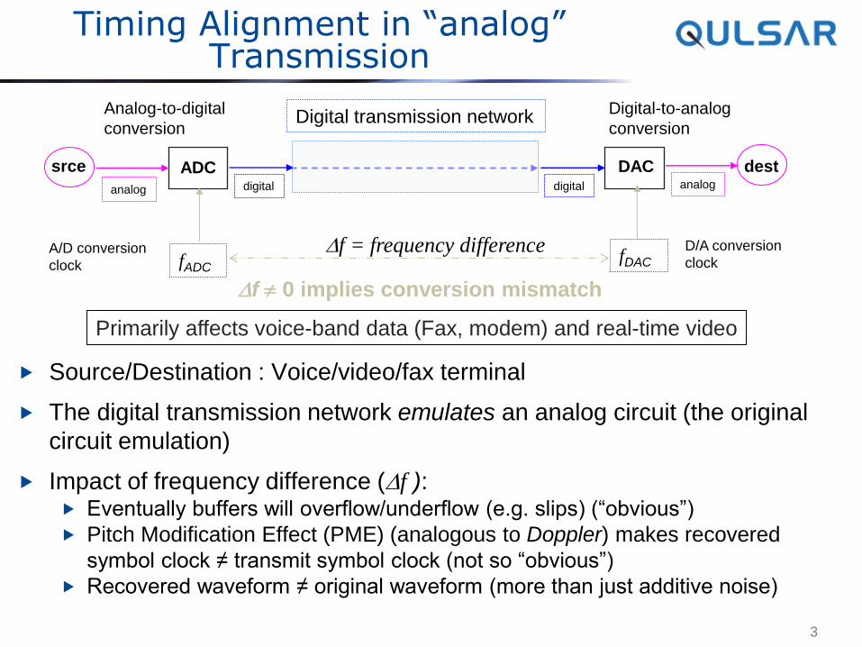
Timing Alignment in “analog” Transmission

Source/Destination : Voice/video/fax terminal

The digital transmission network emulates an analog circuit (the original

circuit emulation)

Impact of frequency difference (Df ): Eventually buffers will overflow/underflow (e.g. slips) (“obvious”)

Pitch Modification Effect (PME) (analogous to Doppler) makes recovered

symbol clock ≠ transmit symbol clock (not so “obvious”)

Recovered waveform ≠ original waveform (more than just additive noise)

3

ADC srce

Analog-to-digital

conversion

analog digital

DAC dest

Digital-to-analog

conversion

analog digital

Digital transmission network

fADC fDAC

Df = frequency difference D/A conversion

clock A/D conversion

clock

Df 0 implies conversion mismatch

Primarily affects voice-band data (Fax, modem) and real-time video

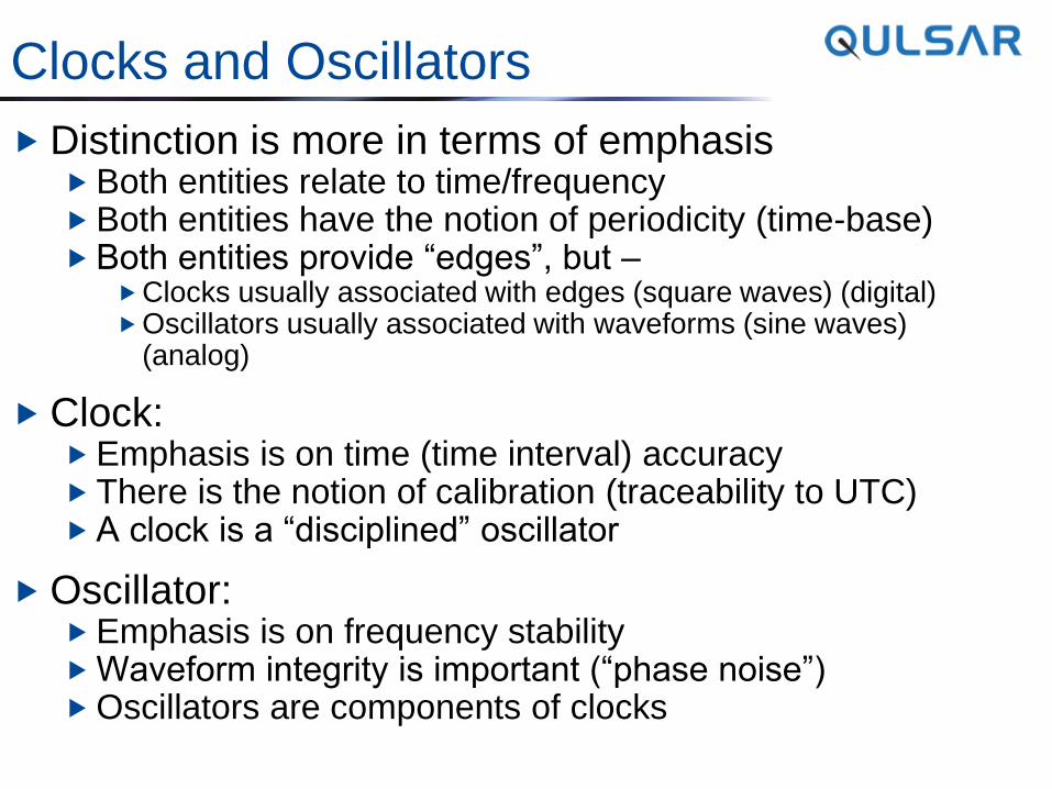
Clocks and Oscillators

Distinction is more in terms of emphasis Both entities relate to time/frequency Both entities have the notion of periodicity (time-base) Both entities provide “edges”, but –

Clocks usually associated with edges (square waves) (digital) Oscillators usually associated with waveforms (sine waves)

(analog)

Clock: Emphasis is on time (time interval) accuracy There is the notion of calibration (traceability to UTC) A clock is a “disciplined” oscillator

Oscillator: Emphasis is on frequency stability Waveform integrity is important (“phase noise”) Oscillators are components of clocks

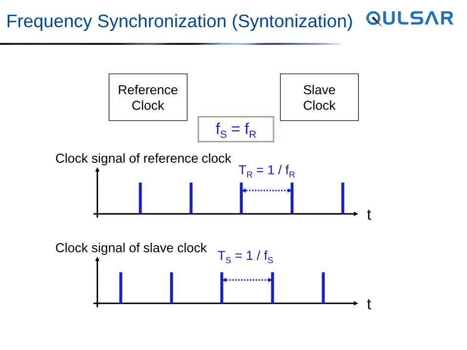
Frequency Synchronization (Syntonization)

Reference

Clock

t

t

Clock signal of reference clock

Clock signal of slave clock

Slave

Clock

TR = 1 / fR

TS = 1 / fS

fS = fR

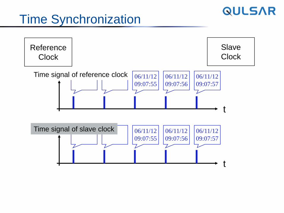
Time Synchronization

Reference

Clock

t

t

Slave

Clock

06/11/12

09:07:56

06/11/12

09:07:57

06/11/12

09:07:55

06/11/12

09:07:55

06/11/12

09:07:56

06/11/12

09:07:57

Time signal of reference clock

Time signal of slave clock

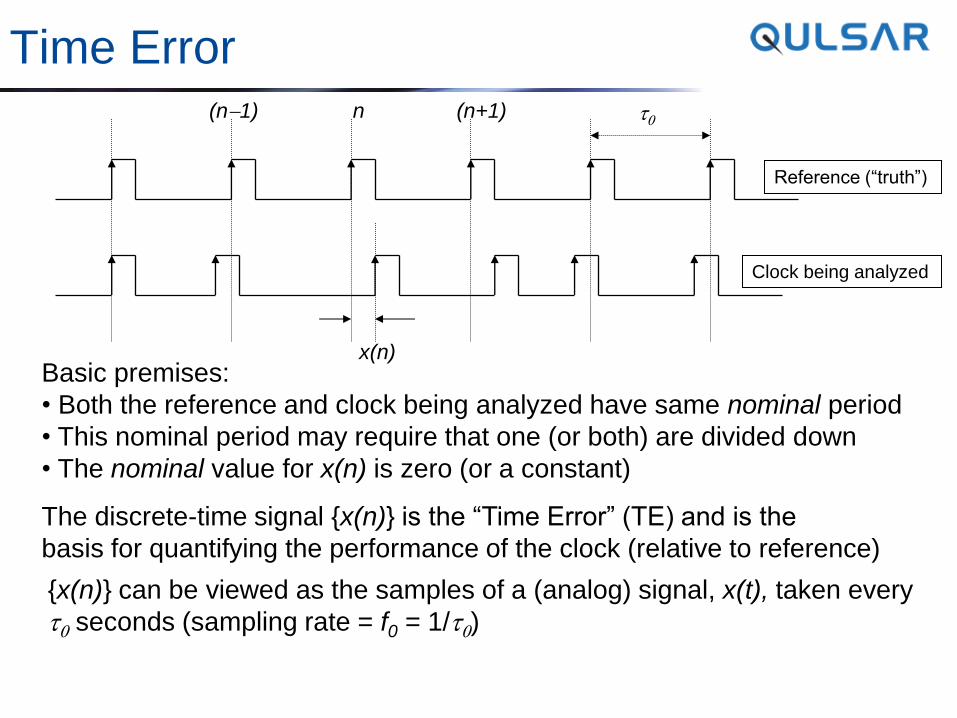
Time Error

Reference (“truth”)

Clock being analyzed

t0 n (n+1) (n-1)

x(n) Basic premises:

• Both the reference and clock being analyzed have same nominal period

• This nominal period may require that one (or both) are divided down

• The nominal value for x(n) is zero (or a constant)

The discrete-time signal {x(n)} is the “Time Error” (TE) and is the

basis for quantifying the performance of the clock (relative to reference)

{x(n)} can be viewed as the samples of a (analog) signal, x(t), taken every

t0 seconds (sampling rate = f0 = 1/t0)

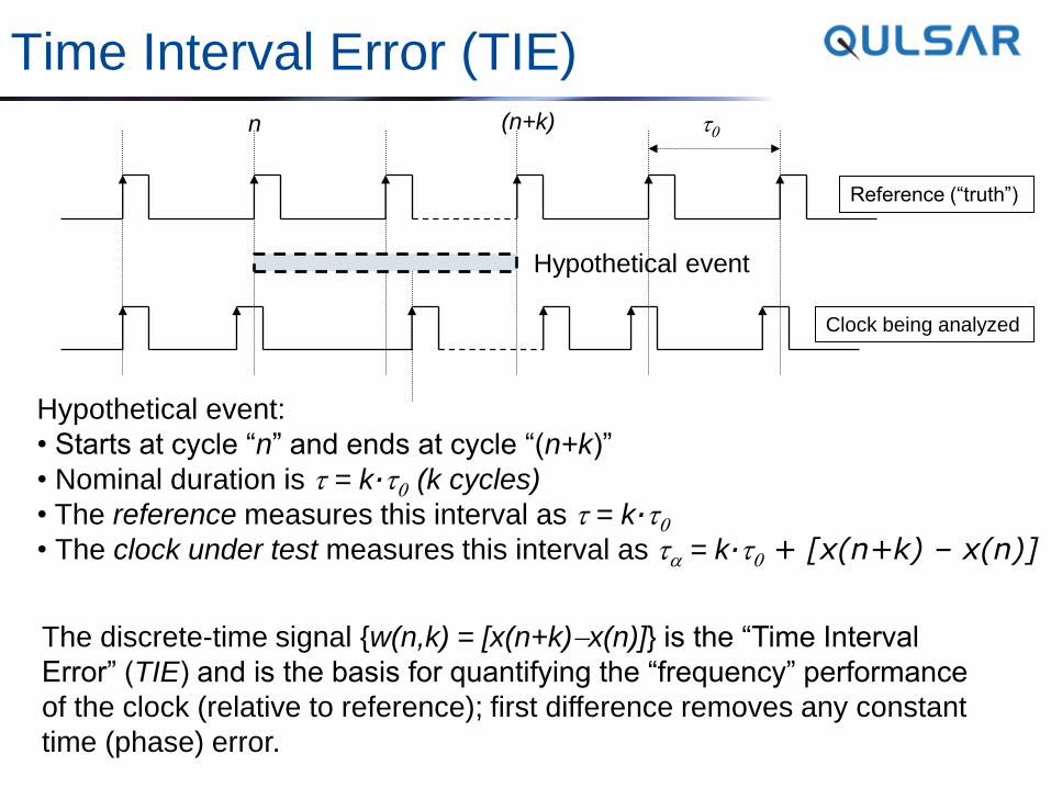
Time Interval Error (TIE)

Reference (“truth”)

Clock being analyzed

t0 n (n+k)

Hypothetical event:

• Starts at cycle “n” and ends at cycle “(n+k)”

• Nominal duration is t = k∙t0 (k cycles)

• The reference measures this interval as t = k∙t0 • The clock under test measures this interval as ta = k∙t0 + [x(n+k) – x(n)]

The discrete-time signal {w(n,k) = [x(n+k)-x(n)]} is the “Time Interval

Error” (TIE) and is the basis for quantifying the “frequency” performance

of the clock (relative to reference); first difference removes any constant

time (phase) error.

Hypothetical event

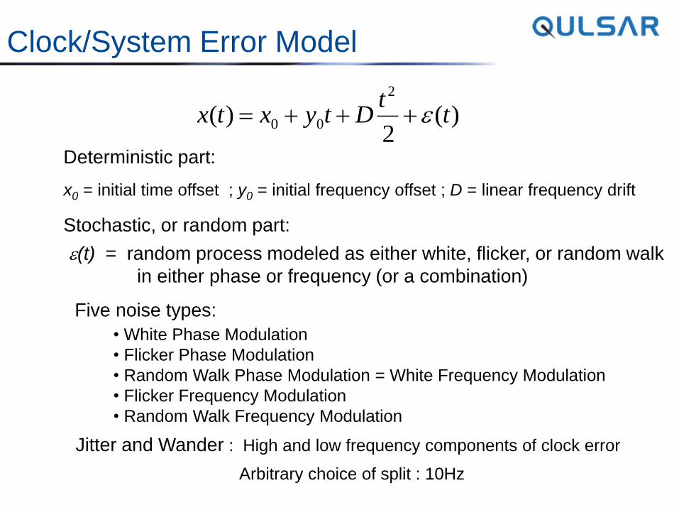
Clock/System Error Model

)(2

)(2

00 tt

Dtyxtx

x0 = initial time offset ; y0 = initial frequency offset ; D = linear frequency drift

Deterministic part:

Stochastic, or random part:

(t) = random process modeled as either white, flicker, or random walk

in either phase or frequency (or a combination)

Five noise types:

• White Phase Modulation

• Flicker Phase Modulation

• Random Walk Phase Modulation = White Frequency Modulation

• Flicker Frequency Modulation

• Random Walk Frequency Modulation

Jitter and Wander : High and low frequency components of clock error

Arbitrary choice of split : 10Hz

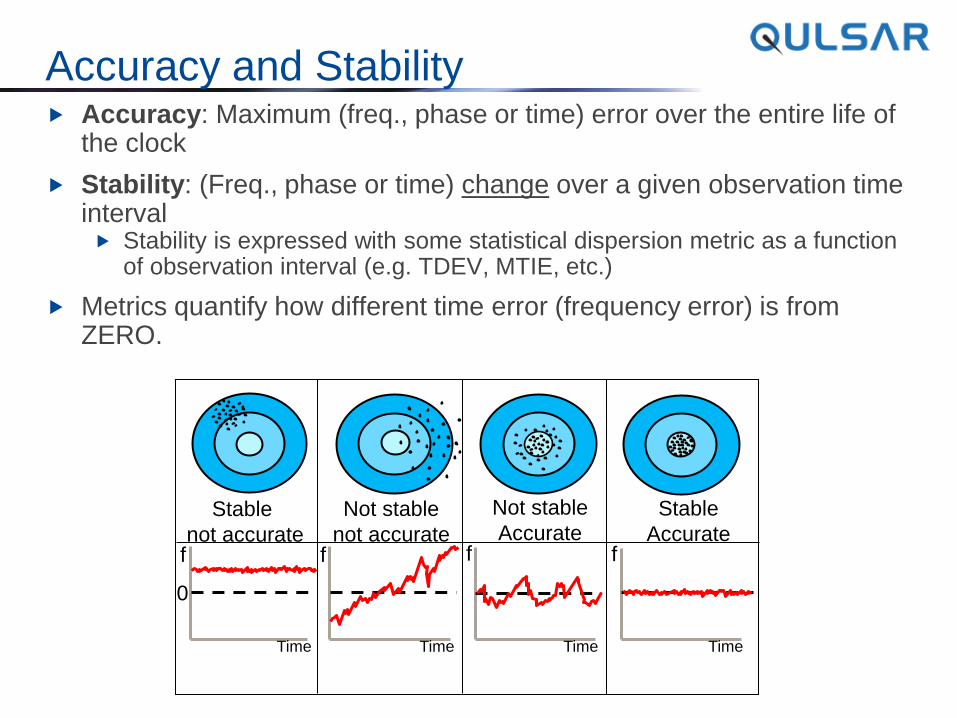
Accuracy and Stability Accuracy: Maximum (freq., phase or time) error over the entire life of

the clock

Stability: (Freq., phase or time) change over a given observation time interval Stability is expressed with some statistical dispersion metric as a function

of observation interval (e.g. TDEV, MTIE, etc.)

Metrics quantify how different time error (frequency error) is from ZERO.

Stable

not accurate

Not stable

not accurate

Not stable

Accurate Stable

Accurate

Time Time Time Time

0

f f f f

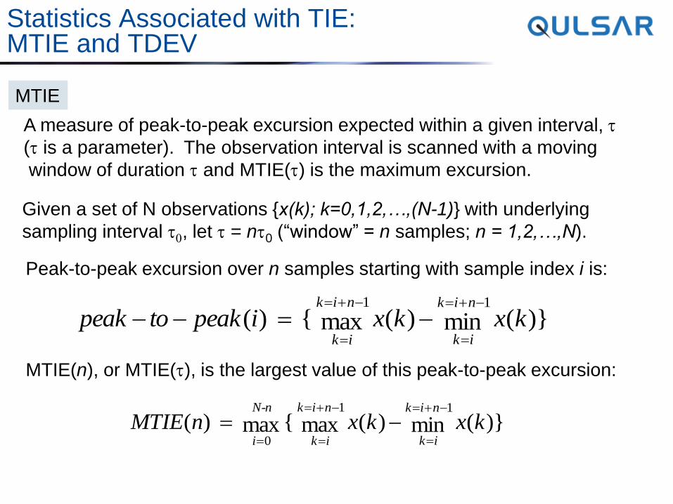
Statistics Associated with TIE: MTIE and TDEV

MTIE

A measure of peak-to-peak excursion expected within a given interval, t

(t is a parameter). The observation interval is scanned with a moving

window of duration t and MTIE(t) is the maximum excursion.

Given a set of N observations {x(k); k=0,1,2,…,(N-1)} with underlying

sampling interval t0, let t = nt0 (“window” = n samples; n = 1,2,…,N).

Peak-to-peak excursion over n samples starting with sample index i is:

)}(min)(max { )(11

kxkxipeaktopeaknik

ik

nik

ik

-

-

---

MTIE(n), or MTIE(t), is the largest value of this peak-to-peak excursion:

)}(min)(max { max )(11

0

kxkxnMTIEnik

ik

nik

ik

N-n

i

-

-

-

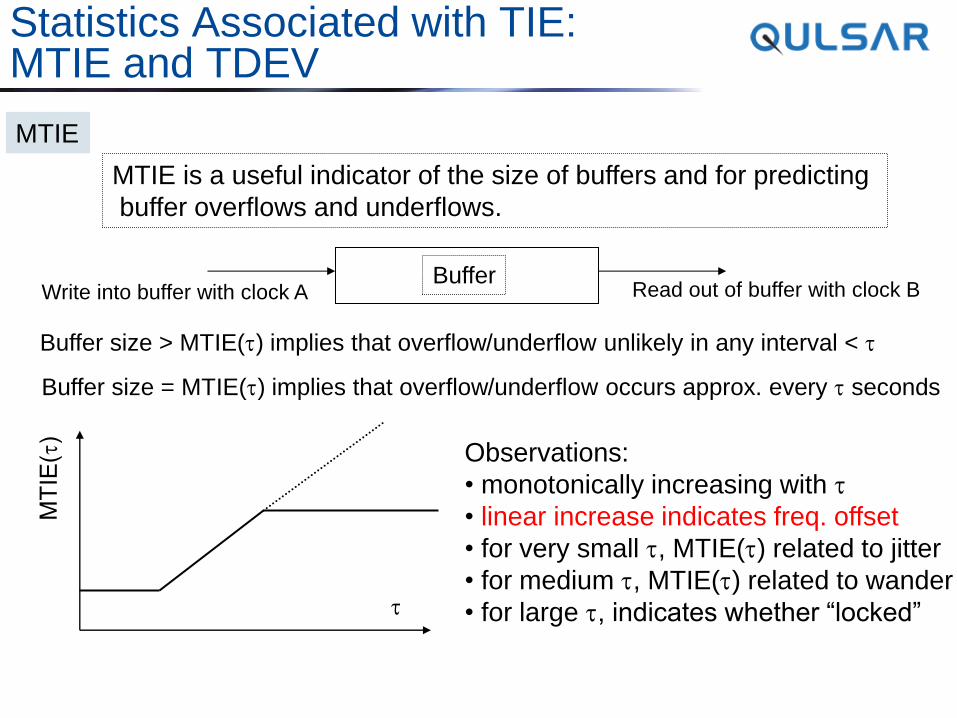
Statistics Associated with TIE: MTIE and TDEV

MTIE

MTIE is a useful indicator of the size of buffers and for predicting

buffer overflows and underflows.

Buffer Write into buffer with clock A Read out of buffer with clock B

Buffer size > MTIE(t) implies that overflow/underflow unlikely in any interval < t

Buffer size = MTIE(t) implies that overflow/underflow occurs approx. every t seconds

t

Observations:

• monotonically increasing with t

• linear increase indicates freq. offset

• for very small t, MTIE(t) related to jitter

• for medium t, MTIE(t) related to wander

• for large t, indicates whether “locked”

Statistics Associated with TIE: MTIE and TDEV

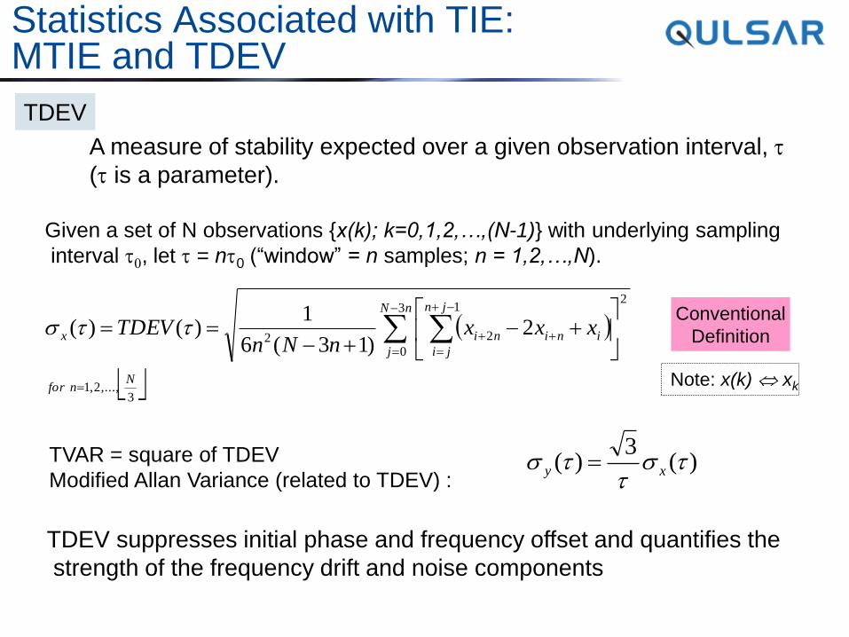
TDEV

A measure of stability expected over a given observation interval, t

(t is a parameter).

Given a set of N observations {x(k); k=0,1,2,…,(N-1)} with underlying sampling

interval t0, let t = nt0 (“window” = n samples; n = 1,2,…,N).

3,...,2,1

3

0

21

222

)13(6

1)()(

Nnfor

nN

j

jn

ji

ininix xxxnNn

TDEV

-

-

-

- tt

Conventional

Definition

TVAR = square of TDEV

Modified Allan Variance (related to TDEV) : )(

3)( t

tt xy

Note: x(k) xk

TDEV suppresses initial phase and frequency offset and quantifies the

strength of the frequency drift and noise components

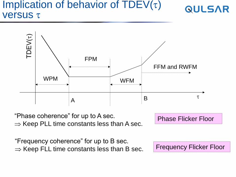
Implication of behavior of TDEV(t) versus t

t

WPM

FPM

WFM

FFM and RWFM

A B

“Phase coherence” for up to A sec.

Keep PLL time constants less than A sec.

“Frequency coherence” for up to B sec.

Keep FLL time constants less than B sec.

Phase Flicker Floor

Frequency Flicker Floor

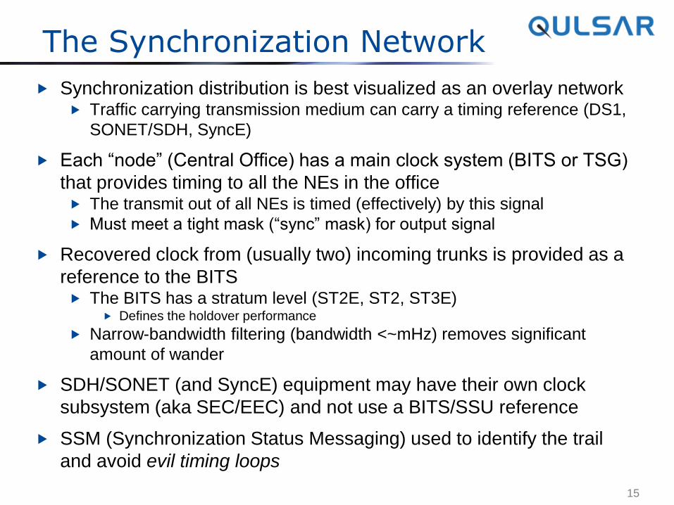
The Synchronization Network

Synchronization distribution is best visualized as an overlay network Traffic carrying transmission medium can carry a timing reference (DS1,

SONET/SDH, SyncE)

Each “node” (Central Office) has a main clock system (BITS or TSG)

that provides timing to all the NEs in the office The transmit out of all NEs is timed (effectively) by this signal

Must meet a tight mask (“sync” mask) for output signal

Recovered clock from (usually two) incoming trunks is provided as a

reference to the BITS The BITS has a stratum level (ST2E, ST2, ST3E)

Defines the holdover performance

Narrow-bandwidth filtering (bandwidth <~mHz) removes significant

amount of wander

SDH/SONET (and SyncE) equipment may have their own clock

subsystem (aka SEC/EEC) and not use a BITS/SSU reference

SSM (Synchronization Status Messaging) used to identify the trail

and avoid evil timing loops

15

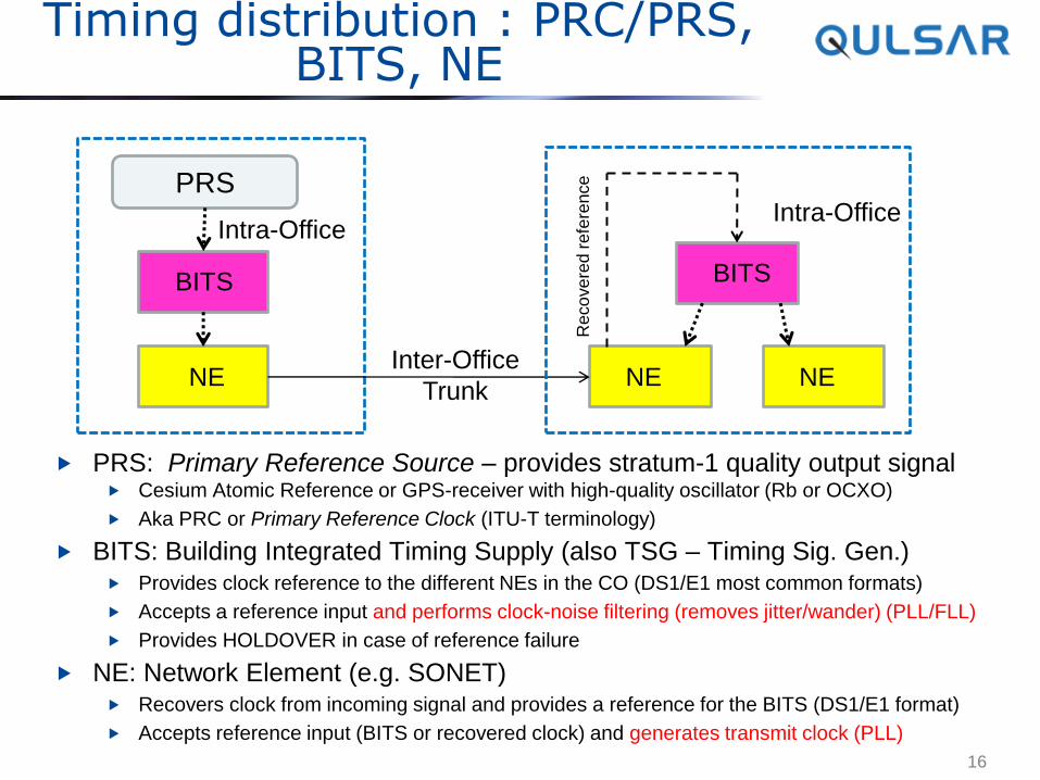
Timing distribution : PRC/PRS, BITS, NE

PRS: Primary Reference Source – provides stratum-1 quality output signal Cesium Atomic Reference or GPS-receiver with high-quality oscillator (Rb or OCXO)

Aka PRC or Primary Reference Clock (ITU-T terminology)

BITS: Building Integrated Timing Supply (also TSG – Timing Sig. Gen.) Provides clock reference to the different NEs in the CO (DS1/E1 most common formats)

Accepts a reference input and performs clock-noise filtering (removes jitter/wander) (PLL/FLL)

Provides HOLDOVER in case of reference failure

NE: Network Element (e.g. SONET) Recovers clock from incoming signal and provides a reference for the BITS (DS1/E1 format)

Accepts reference input (BITS or recovered clock) and generates transmit clock (PLL)

16

PRS

Intra-Office

Inter-Office

Trunk

BITS BITS

NE NE NE

Intra-Office

Reco

ve

red

refe

ren

ce

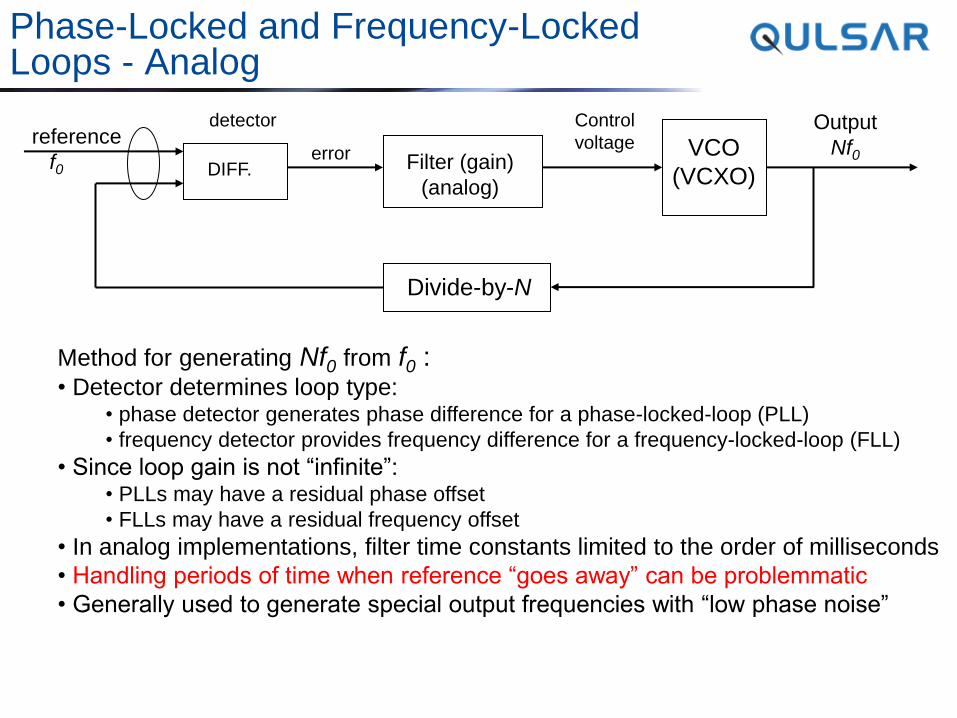
Phase-Locked and Frequency-Locked Loops - Analog

DIFF.

detector reference

Filter (gain)

(analog)

VCO

(VCXO) error

Control

voltage

Divide-by-N

f0

Output

Nf0

Method for generating Nf0 from f0 : • Detector determines loop type:

• phase detector generates phase difference for a phase-locked-loop (PLL)

• frequency detector provides frequency difference for a frequency-locked-loop (FLL)

• Since loop gain is not “infinite”: • PLLs may have a residual phase offset

• FLLs may have a residual frequency offset

• In analog implementations, filter time constants limited to the order of milliseconds

• Handling periods of time when reference “goes away” can be problemmatic

• Generally used to generate special output frequencies with “low phase noise”

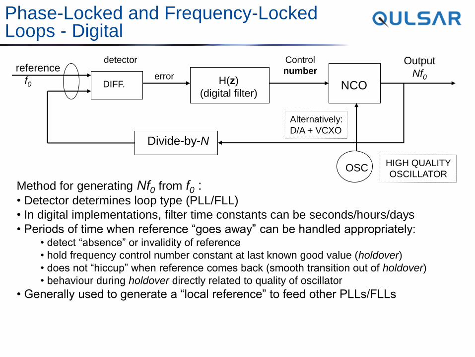
Phase-Locked and Frequency-Locked Loops - Digital

DIFF.

detector reference

H(z)

(digital filter) NCO

error

Control

number

Divide-by-N

f0

Output

Nf0

Method for generating Nf0 from f0 : • Detector determines loop type (PLL/FLL)

• In digital implementations, filter time constants can be seconds/hours/days

• Periods of time when reference “goes away” can be handled appropriately: • detect “absence” or invalidity of reference

• hold frequency control number constant at last known good value (holdover)

• does not “hiccup” when reference comes back (smooth transition out of holdover)

• behaviour during holdover directly related to quality of oscillator

• Generally used to generate a “local reference” to feed other PLLs/FLLs

OSC HIGH QUALITY

OSCILLATOR

Alternatively:

D/A + VCXO

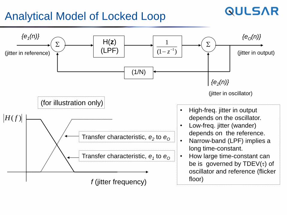
Analytical Model of Locked Loop

S

{e1(n)} H(z)

(LPF) )1(

11-- z

S

(1/N)

{eO(n)}

{e2(n)}

f (jitter frequency)

Transfer characteristic, e2 to eO

Transfer characteristic, e1 to eO

• High-freq. jitter in output

depends on the oscillator.

• Low-freq. jitter (wander)

depends on the reference.

• Narrow-band (LPF) implies a

long time-constant.

• How large time-constant can

be is governed by TDEV(t) of

oscillator and reference (flicker

floor)

(jitter in reference)

(jitter in oscillator)

(jitter in output)

)( fH

(for illustration only)

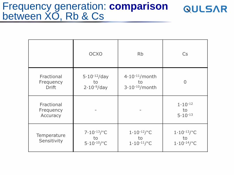
Frequency generation: comparison between XO, Rb & Cs

OCXO Rb Cs

Fractional Frequency

Drift

5·10-12/day to

2·10-9/day

4·10-11/month to

3·10-10/month 0

Fractional Frequency Accuracy

- - 1·10-12

to 5·10-13

Temperature Sensitivity

7·10-13/°C

to 5·10-10/°C

1·10-12/°C

to 1·10-11/°C

1·10-13/°C

to 1·10-14/°C

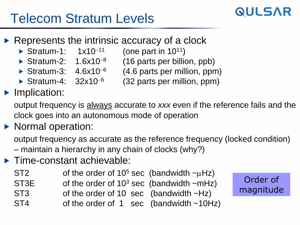
Telecom Stratum Levels

Represents the intrinsic accuracy of a clock Stratum-1: 1x10-11 (one part in 1011)

Stratum-2: 1.6x10-8 (16 parts per billion, ppb)

Stratum-3: 4.6x10-6 (4.6 parts per million, ppm)

Stratum-4: 32x10-6 (32 parts per million, ppm)

Implication:

output frequency is always accurate to xxx even if the reference fails and the

clock goes into an autonomous mode of operation

Normal operation:

output frequency as accurate as the reference frequency (locked condition)

– maintain a hierarchy in any chain of clocks (why?)

Time-constant achievable:

ST2 of the order of 105 sec (bandwidth ~mHz)

ST3E of the order of 103 sec (bandwidth ~mHz)

ST3 of the order of 10 sec (bandwidth ~Hz)

ST4 of the order of 1 sec (bandwidth ~10Hz)

Order of magnitude

Thank You!

Questions?

Kishan Shenoi

CTO, Qulsar, LLC

kshenoi@qulsar.com

Back-up Slides follow

Special thanks to Dominik Schneuwly of OSA and Chip Webb of Ixia/Anue for permission to include slides from

prior WSTS/ITSF and other presentations

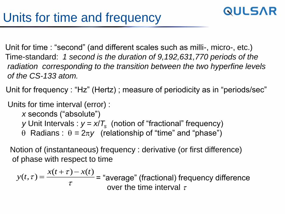
Units for time and frequency

Unit for time : “second” (and different scales such as milli-, micro-, etc.)

Time-standard: 1 second is the duration of 9,192,631,770 periods of the

radiation corresponding to the transition between the two hyperfine levels

of the CS-133 atom.

Unit for frequency : “Hz” (Hertz) ; measure of periodicity as in “periods/sec”

Units for time interval (error) :

x seconds (“absolute”)

y Unit Intervals : y = x/Ts (notion of “fractional” frequency)

Radians : = 2y (relationship of “time” and “phase”)

Notion of (instantaneous) frequency : derivative (or first difference)

of phase with respect to time

t

tt

)()(),(

txtxty

- = “average” (fractional) frequency difference

over the time interval t

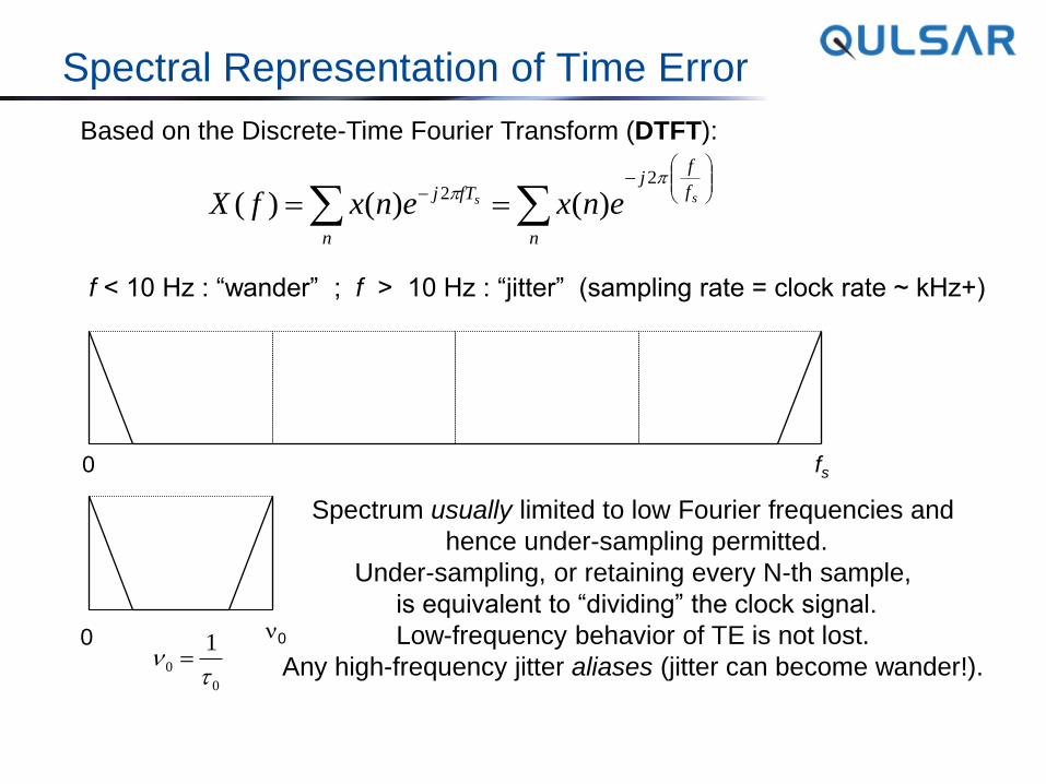
Spectral Representation of Time Error

Based on the Discrete-Time Fourier Transform (DTFT):

-

-

n

f

fj

n

fTj ss enxenxfX

2

2)()()(

f < 10 Hz : “wander” ; f > 10 Hz : “jitter” (sampling rate = clock rate ~ kHz+)

0

0

fs

n0

Spectrum usually limited to low Fourier frequencies and

hence under-sampling permitted.

Under-sampling, or retaining every N-th sample,

is equivalent to “dividing” the clock signal.

Low-frequency behavior of TE is not lost.

Any high-frequency jitter aliases (jitter can become wander!). 0

0

1

tn

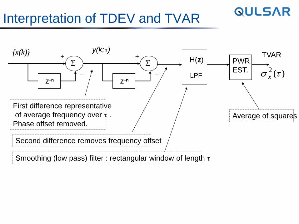
Interpretation of TDEV and TVAR

Z-n

S +

- Z-n

S +

-

{x(k)} H(z)

LPF

PWR

EST.

First difference representative

of average frequency over t .

Phase offset removed.

y(k;t)

Second difference removes frequency offset

Smoothing (low pass) filter : rectangular window of length t

Average of squares

TVAR

)(2 t x

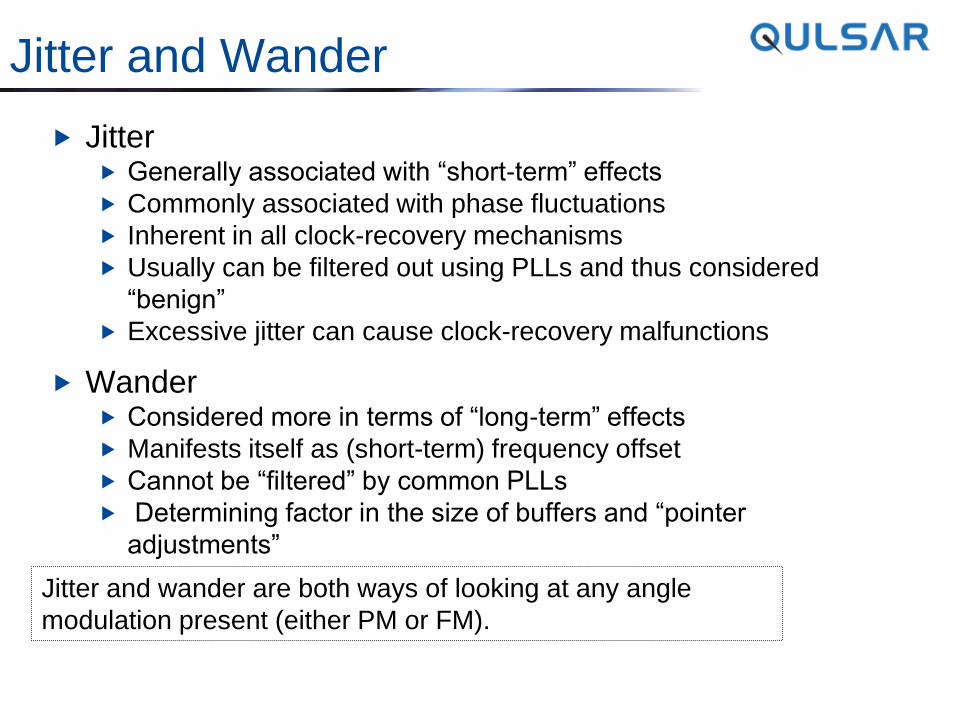
Jitter and Wander

Jitter Generally associated with “short-term” effects

Commonly associated with phase fluctuations

Inherent in all clock-recovery mechanisms

Usually can be filtered out using PLLs and thus considered

“benign”

Excessive jitter can cause clock-recovery malfunctions

Wander Considered more in terms of “long-term” effects

Manifests itself as (short-term) frequency offset

Cannot be “filtered” by common PLLs

Determining factor in the size of buffers and “pointer

adjustments”

Jitter and wander are both ways of looking at any angle

modulation present (either PM or FM).

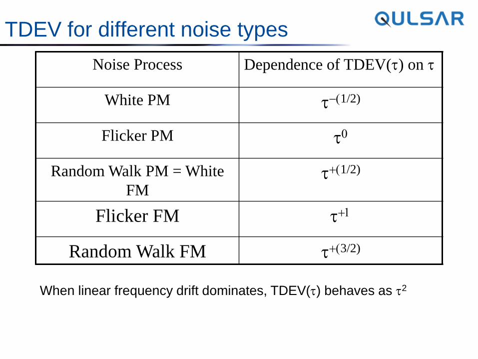
TDEV for different noise types

Noise Process Dependence of TDEV(t) on t

White PM t-1/2)

Flicker PM t0

Random Walk PM = White

FM t1/2)

Flicker FM t1

Random Walk FM t3/2)

When linear frequency drift dominates, TDEV(t) behaves as t2

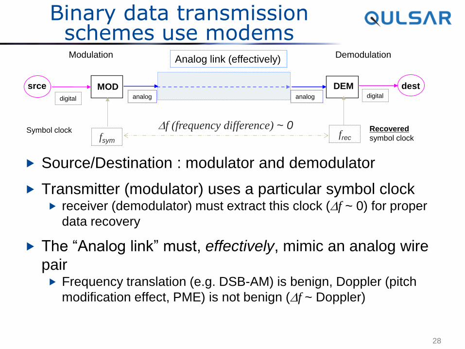
Binary data transmission schemes use modems

Source/Destination : modulator and demodulator

Transmitter (modulator) uses a particular symbol clock receiver (demodulator) must extract this clock (Df ~ 0) for proper

data recovery

The “Analog link” must, effectively, mimic an analog wire

pair Frequency translation (e.g. DSB-AM) is benign, Doppler (pitch

modification effect, PME) is not benign (Df ~ Doppler)

28

MOD srce

Modulation

digital analog

DEM dest

Demodulation

digital analog

Analog link (effectively)

fsym frec

Df (frequency difference) ~ 0 Recovered

symbol clock Symbol clock

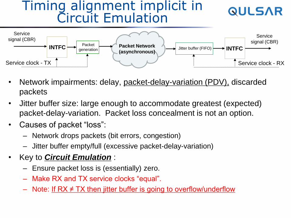
Timing alignment implicit in Circuit Emulation

• Network impairments: delay, packet-delay-variation (PDV), discarded

packets

• Jitter buffer size: large enough to accommodate greatest (expected)

packet-delay-variation. Packet loss concealment is not an option.

• Causes of packet “loss”:

– Network drops packets (bit errors, congestion)

– Jitter buffer empty/full (excessive packet-delay-variation)

• Key to Circuit Emulation :

– Ensure packet loss is (essentially) zero.

– Make RX and TX service clocks “equal”.

– Note: If RX ≠ TX then jitter buffer is going to overflow/underflow

INTFC Packet

generation Packet Network

(asynchronous) Jitter buffer (FIFO) INTFC

Service

signal (CBR) Service

signal (CBR)

Service clock - RX Service clock - TX

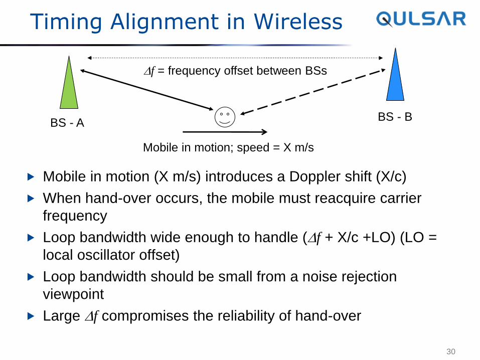
Timing Alignment in Wireless

Mobile in motion (X m/s) introduces a Doppler shift (X/c)

When hand-over occurs, the mobile must reacquire carrier

frequency

Loop bandwidth wide enough to handle (Df + X/c +LO) (LO =

local oscillator offset)

Loop bandwidth should be small from a noise rejection

viewpoint

Large Df compromises the reliability of hand-over

30

BS - A BS - B

Df = frequency offset between BSs

Mobile in motion; speed = X m/s

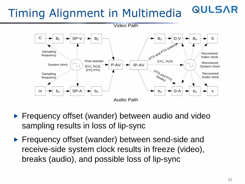
Timing Alignment in Multimedia

Frequency offset (wander) between audio and video

sampling results in loss of lip-sync

Frequency offset (wander) between send-side and

receive-side system clock results in freeze (video),

breaks (audio), and possible loss of lip-sync

31

Video Path

Audio Path

C

m

B1 B2

IP-AV

B3 B4

b4b3b2b1

SP-V

SP-A

P-AV

D-V

D-A

S

s

System clock

Sampling

frequency

Sampling

frequency

Time-stamps STC, PCR

Recovered

Video clock

Recovered

Audio clock

Recovered

System clock

DTS and PTS (v

ideo)

DTS and PTS

(audio)

STC, PCR,

DTS PTS

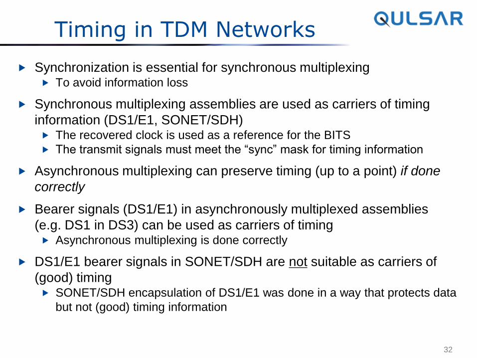
Timing in TDM Networks

Synchronization is essential for synchronous multiplexing To avoid information loss

Synchronous multiplexing assemblies are used as carriers of timing

information (DS1/E1, SONET/SDH) The recovered clock is used as a reference for the BITS

The transmit signals must meet the “sync” mask for timing information

Asynchronous multiplexing can preserve timing (up to a point) if done

correctly

Bearer signals (DS1/E1) in asynchronously multiplexed assemblies

(e.g. DS1 in DS3) can be used as carriers of timing Asynchronous multiplexing is done correctly

DS1/E1 bearer signals in SONET/SDH are not suitable as carriers of

(good) timing SONET/SDH encapsulation of DS1/E1 was done in a way that protects data

but not (good) timing information

32

Timing Issues in Next Generation Networks

Next generation networks are based on packet switching

as opposed to circuit-switched (i.e. based on TDM)

Significant impact of variable delay (packet delay

variation)

Timing requirements remain. Going “IP” does not mean

that real-time services no longer need synchronization!

Transition Phase: Hybrid Networks (IP/TDM islands)

Circuit Emulation

Timing over Packet Networks (packet-based methods) PTP, NTP, adaptive clock recovery

The testing challenge Metrics for packet-based timing methods (quantifying PDV)

33

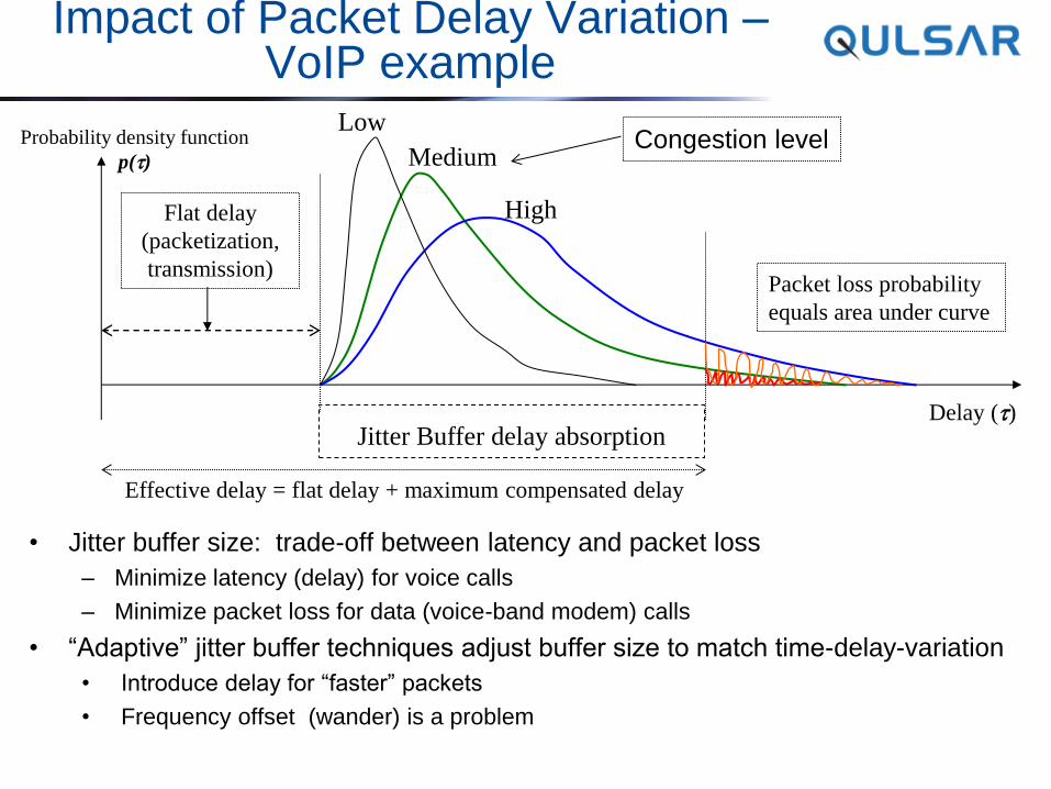
Impact of Packet Delay Variation – VoIP example

• Jitter buffer size: trade-off between latency and packet loss

– Minimize latency (delay) for voice calls

– Minimize packet loss for data (voice-band modem) calls

• “Adaptive” jitter buffer techniques adjust buffer size to match time-delay-variation

• Introduce delay for “faster” packets

• Frequency offset (wander) is a problem

Delay (t)

Flat delay

(packetization,

transmission)

Jitter Buffer delay absorption

Packet loss probability

equals area under curve

Effective delay = flat delay + maximum compensated delay

Low

Medium

High

Congestion level Probability density function

p(t)

Principles of Packet-based timing methods

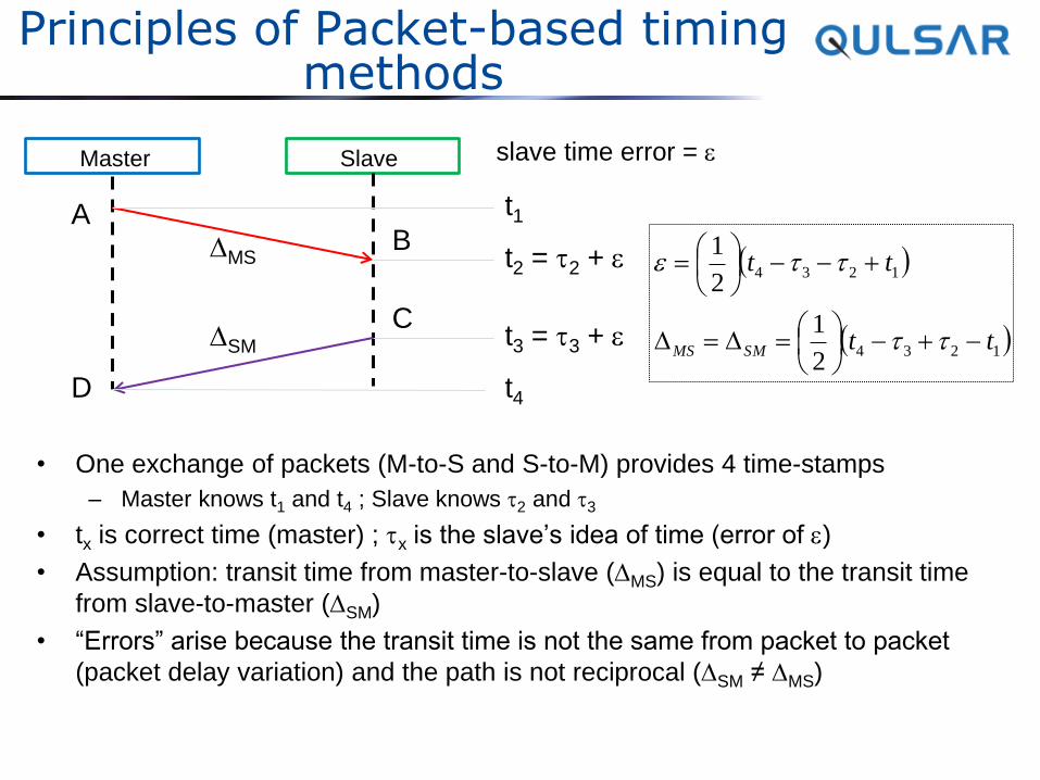
• One exchange of packets (M-to-S and S-to-M) provides 4 time-stamps

– Master knows t1 and t4 ; Slave knows t2 and t3

• tx is correct time (master) ; tx is the slave’s idea of time (error of )

• Assumption: transit time from master-to-slave (DMS) is equal to the transit time

from slave-to-master (DSM)

• “Errors” arise because the transit time is not the same from packet to packet

(packet delay variation) and the path is not reciprocal (DSM ≠ DMS)

Master Slave

A B

C

D

DMS

DSM

t1

t2 = t2 +

t3 = t3 +

t4

slave time error =

1234

1234

2

1

2

1

tt

tt

SMMS --

DD

--

tt

tt

PTP and NTP

Similar in principle, differences in details Both use 4 time-stamps (basic two-way-time-transfer principle is

common to both)

Standards: NTP: developed by IETF (RFC 5905) (now V4)

PTP: developed by IEEE : IEEE-1588-V2 geared to telecom req.

Origins: NTP developed to provide time-of-day to PCs, workstations, etc.,

over the big bad Internet

PTP developed to provide alignment of robots on a manufacturing

floor

Source and Sink: PTP: each “slave” has one “master” (one master per community)

NTP: each “client” can query multiple “servers” and do some fancy

averaging (the “community” is not well defined)

36

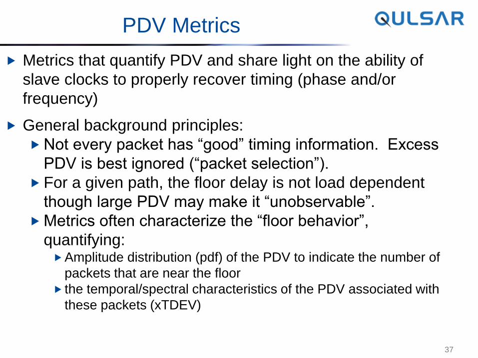
PDV Metrics

Metrics that quantify PDV and share light on the ability of

slave clocks to properly recover timing (phase and/or

frequency)

General background principles:

Not every packet has “good” timing information. Excess

PDV is best ignored (“packet selection”).

For a given path, the floor delay is not load dependent

though large PDV may make it “unobservable”.

Metrics often characterize the “floor behavior”,

quantifying: Amplitude distribution (pdf) of the PDV to indicate the number of

packets that are near the floor

the temporal/spectral characteristics of the PDV associated with

these packets (xTDEV)

37

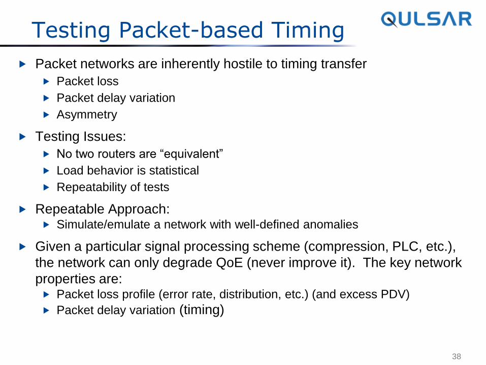
Testing Packet-based Timing

Packet networks are inherently hostile to timing transfer

Packet loss

Packet delay variation

Asymmetry

Testing Issues:

No two routers are “equivalent”

Load behavior is statistical

Repeatability of tests

Repeatable Approach: Simulate/emulate a network with well-defined anomalies

Given a particular signal processing scheme (compression, PLC, etc.),

the network can only degrade QoE (never improve it). The key network

properties are: Packet loss profile (error rate, distribution, etc.) (and excess PDV)

Packet delay variation (timing)

38

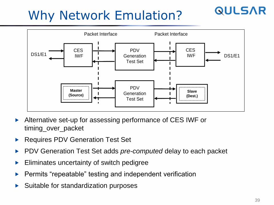
Why Network Emulation?

Alternative set-up for assessing performance of CES IWF or

timing_over_packet

Requires PDV Generation Test Set

PDV Generation Test Set adds pre-computed delay to each packet

Eliminates uncertainty of switch pedigree

Permits “repeatable” testing and independent verification

Suitable for standardization purposes

39

PDV Generation

Test Set

CES IWF DS1/E1

PDV Generation

Test Set

DS1/E1

CES IWF

Packet Interface Packet Interface

Master

(Source) Slave

(Dest.)

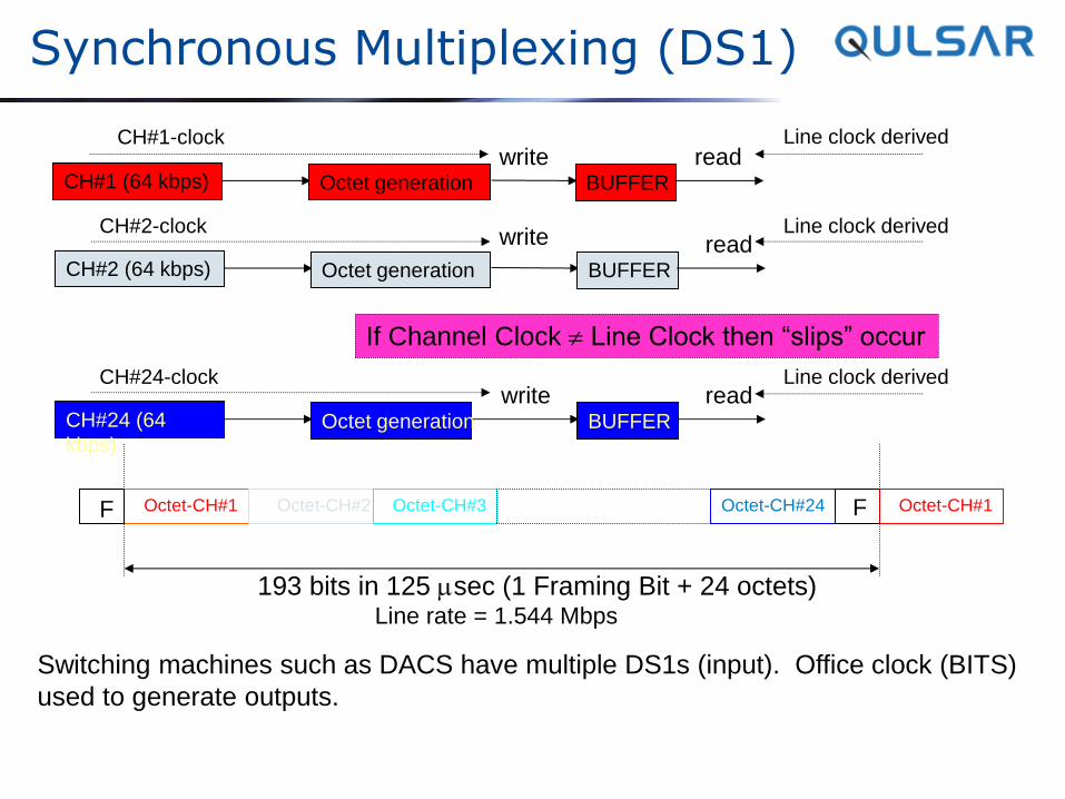
Synchronous Multiplexing (DS1)

193 bits in 125 msec (1 Framing Bit + 24 octets)

F F Octet-CH#1 Octet-CH#2 Octet-CH#24 Octet-CH#3 Octet-CH#1

CH#1 (64 kbps) Octet generation BUFFER

write read CH#1-clock

Line rate = 1.544 Mbps

Line clock derived

CH#2 (64 kbps) Octet generation BUFFER

write read CH#2-clock Line clock derived

CH#24 (64

kbps) Octet generation BUFFER

write read CH#24-clock Line clock derived

If Channel Clock Line Clock then “slips” occur

Switching machines such as DACS have multiple DS1s (input). Office clock (BITS)

used to generate outputs.

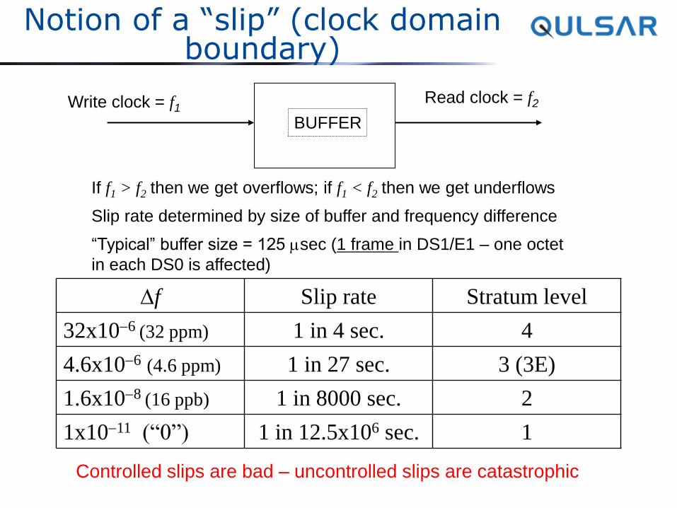
Notion of a “slip” (clock domain boundary)

BUFFER

Write clock = f1 Read clock = f2

If f1 > f2 then we get overflows; if f1 < f2 then we get underflows

Slip rate determined by size of buffer and frequency difference

“Typical” buffer size = 125 msec (1 frame in DS1/E1 – one octet

in each DS0 is affected)

Df Slip rate Stratum level

32x10-6 (32 ppm) 1 in 4 sec. 4

4.6x10-6 (4.6 ppm) 1 in 27 sec. 3 (3E)

1.6x10-8 (16 ppb) 1 in 8000 sec. 2

1x10-11 (“0”) 1 in 12.5x106 sec. 1

Controlled slips are bad – uncontrolled slips are catastrophic

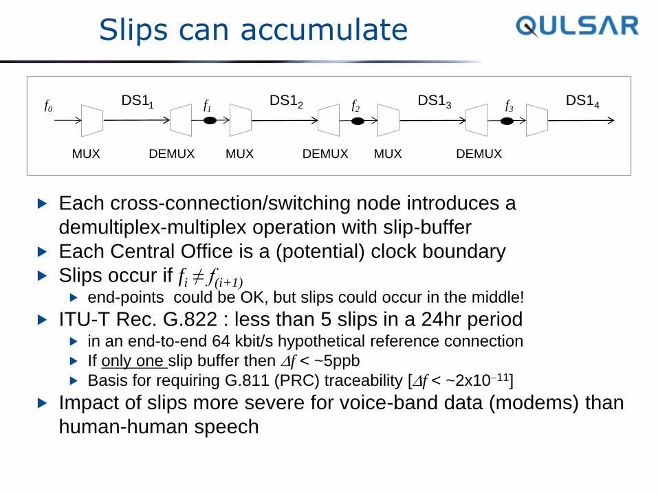
Slips can accumulate

Each cross-connection/switching node introduces a

demultiplex-multiplex operation with slip-buffer

Each Central Office is a (potential) clock boundary

Slips occur if fi ≠ f(i+1) end-points could be OK, but slips could occur in the middle!

ITU-T Rec. G.822 : less than 5 slips in a 24hr period in an end-to-end 64 kbit/s hypothetical reference connection

If only one slip buffer then Df < ~5ppb

Basis for requiring G.811 (PRC) traceability [Df < ~2x10-11]

Impact of slips more severe for voice-band data (modems) than

human-human speech

f0 DS11 f1

DS12 f2

MUX DEMUX MUX DEMUX

DS13 f3

MUX DEMUX

DS14

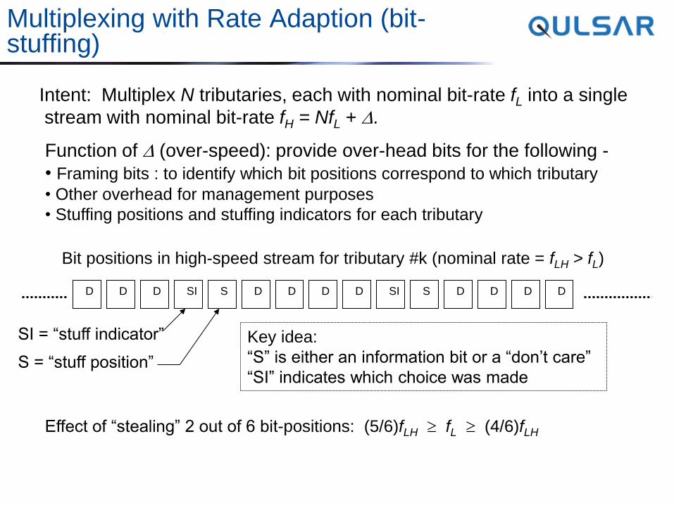
Multiplexing with Rate Adaption (bit-stuffing)

Intent: Multiplex N tributaries, each with nominal bit-rate fL into a single

stream with nominal bit-rate fH = NfL + D.

Function of D (over-speed): provide over-head bits for the following -

• Framing bits : to identify which bit positions correspond to which tributary

• Other overhead for management purposes

• Stuffing positions and stuffing indicators for each tributary

D D D SI S D D D D SI S D D D D

Bit positions in high-speed stream for tributary #k (nominal rate = fLH > fL)

SI = “stuff indicator”

S = “stuff position”

Key idea:

“S” is either an information bit or a “don’t care”

“SI” indicates which choice was made

Effect of “stealing” 2 out of 6 bit-positions: (5/6)fLH fL (4/6)fLH

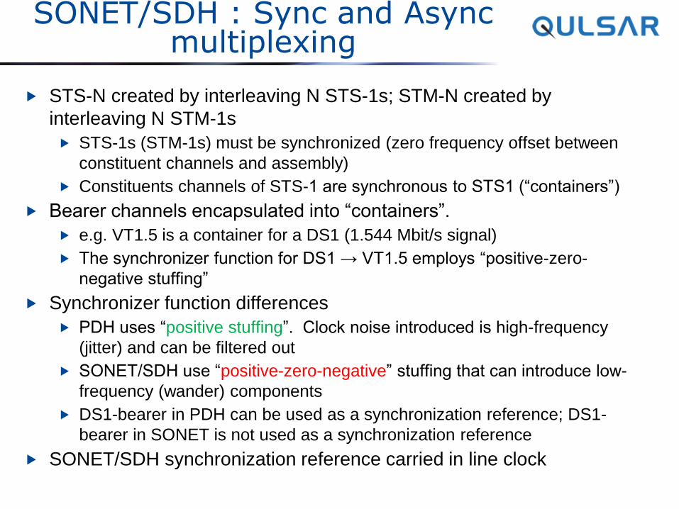
SONET/SDH : Sync and Async multiplexing

STS-N created by interleaving N STS-1s; STM-N created by

interleaving N STM-1s

STS-1s (STM-1s) must be synchronized (zero frequency offset between

constituent channels and assembly)

Constituents channels of STS-1 are synchronous to STS1 (“containers”)

Bearer channels encapsulated into “containers”.

e.g. VT1.5 is a container for a DS1 (1.544 Mbit/s signal)

The synchronizer function for DS1 → VT1.5 employs “positive-zero-

negative stuffing”

Synchronizer function differences

PDH uses “positive stuffing”. Clock noise introduced is high-frequency

(jitter) and can be filtered out

SONET/SDH use “positive-zero-negative” stuffing that can introduce low-

frequency (wander) components

DS1-bearer in PDH can be used as a synchronization reference; DS1-

bearer in SONET is not used as a synchronization reference

SONET/SDH synchronization reference carried in line clock

Standards Bodies, Workshops, Forums

ITU-T – International Telecommunication Union – Telecom Sector (United Nations)

ATIS – Alliance for Telecommunications Industry Solutions

ETSI – European Telecommunications Standards Institute

IEEE – Institute of Electrical and Electronics Engineers

Telcordia – Formerly BellCore

IETF – Internet Engineering Task Force TICTOC – Timing over IP Connection and Transfer of Clock

Relevant Workshops/Forums: NIST - National Institute of Standards and Technology (annual

Workshop on Synch. In Telecom. Systems, WSTS is co-sponsored by Telcordia, ATIS, and IEEE)

ITSF - International Telecom Synchronization Forum

Synchronization in TDM Networks – Key Points

Delivery of information can be compromised by absence of synchronization Especially true for “analog” and CBR signals

Synchronous multiplexing requires that bearer channels and assembly be synchronized Rate adaptation in DS1/E1 achieved by slip buffers; Df ≠ 0 leads to

data corruption SONET/SDH also use synchronous multiplexing to get the higher

bit-rates

Asynchronous multiplexing requires that the bearer channel be rate-adapted (bit stuffing) to channel rate Positive stuffing introduces high-frequency noise (jitter) (PDH) Positive-zero-negative stuffing introduces wander (SDH) Bearer channel clock noise is sum of stuffing noise (filtered) and

assembly clock noise

SONET/SDH bearer signals not suitable as synchronization reference Derived DS1/E1 based on optical line-clock used as a

synchronization reference

Timing Considerations — Packet

• Real-time services require timing (frequency) at conversion points (e.g. A/D and D/A converters; C-to-P conversion points) (regardless of transport mechanisms) – Future requirements may include both frequency and time (“time of

day”)

• Packet Networks may not require timing (frequency) to maintain transport data integrity….. – Data transfer is bursty, with “gaps” and time-delay variation

Frequency offset “absorbed” by jitter buffers; errors caused by overflow/underflow

Buffers can be made large (with a latency penalty)

– Delivery of sync reference to the end-points, for supporting real-time services, is still required and just may be “natural” as in TDM How does an IAD fed by Ethernet get its synch. reference? (SyncE!)

– Common misconception that since transport does not require it, timing is “not necessary” (overlooking requirement of service)

Timing Considerations — TDM

Supporting real-time services require timing (frequency) at the conversion points (e.g. A/D and D/A converters) (regardless of transport mechanisms) Future requirements may include both frequency and time (“Time-of-

Day”)

Circuit Switched Network (“TDM”) requires timing (frequency) in order to maintain transport data integrity Transmitted signal is “continuous”

Frequency offsets “absorbed” by slip buffers (not error free)

Recovered clock from physical layer can be a timing reference Delivery of timing reference to the end-points is straightforward

e.g. DS1 IADs can use loop-timing, deriving timing from the network by using the DS1 recovered clock as a reference**

Synchronizing the transport network indirectly provides the timing required to support real-time services

**: Very Important

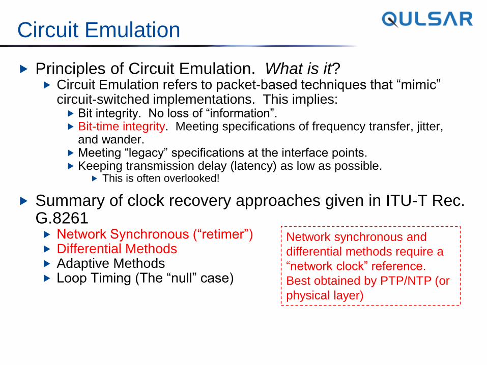
Circuit Emulation

Principles of Circuit Emulation. What is it? Circuit Emulation refers to packet-based techniques that “mimic”

circuit-switched implementations. This implies: Bit integrity. No loss of “information”. Bit-time integrity. Meeting specifications of frequency transfer, jitter,

and wander. Meeting “legacy” specifications at the interface points. Keeping transmission delay (latency) as low as possible.

This is often overlooked!

Summary of clock recovery approaches given in ITU-T Rec. G.8261 Network Synchronous (“retimer”) Differential Methods Adaptive Methods Loop Timing (The “null” case)

Network synchronous and

differential methods require a

“network clock” reference.

Best obtained by PTP/NTP (or

physical layer)

Recap – Timing in NGN

Going “IP” does not mean that real-time services

no longer need synchronization! Timing requirements based on Transport and Service

Transition Phase – Hybrid Networks Increased delay brings its own issues (e.g. echo)

Circuit Emulation

Timing over Packet Networks Two-way time transfer

PTP and NTP

Packet Delay Variation and Metrics

Testing Issues

50

PTP and NTP – some distinctions

Different notion of “Time 0”

Different formats for time-stamps PTP limit : 2-32 s (tenths of nanoseconds)

NTP limit : picoseconds

Initiator: NTP: client initiates interaction. Request to Server who replies.

S-M Query; M-S Response

PTP: Master speaks (twice!), Slave listens and occasionally asks a

question and Master responds. M-S Sync and Follow-up; S-M delay-request and M-S delay-response

PTP has the notion of on-path support – aka transparent

clocks and boundary clocks

PTP community of clocks may have to decide who is

Master (aka Best Master Algorithm)

Different (artificial) limits on packet rate

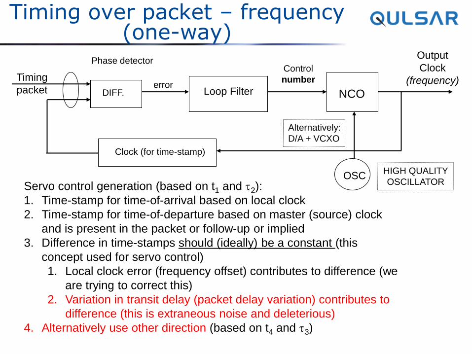
Timing over packet – frequency (one-way)

DIFF.

Phase detector

Timing

packet Loop Filter NCO error

Control

number

Clock (for time-stamp)

Output

Clock

(frequency)

Servo control generation (based on t1 and t2):

1. Time-stamp for time-of-arrival based on local clock

2. Time-stamp for time-of-departure based on master (source) clock

and is present in the packet or follow-up or implied

3. Difference in time-stamps should (ideally) be a constant (this

concept used for servo control)

1. Local clock error (frequency offset) contributes to difference (we

are trying to correct this)

2. Variation in transit delay (packet delay variation) contributes to

difference (this is extraneous noise and deleterious)

4. Alternatively use other direction (based on t4 and t3)

OSC HIGH QUALITY

OSCILLATOR

Alternatively:

D/A + VCXO

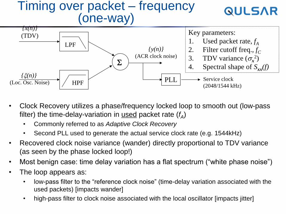
Timing over packet – frequency (one-way)

• Clock Recovery utilizes a phase/frequency locked loop to smooth out (low-pass

filter) the time-delay-variation in used packet rate (fA)

• Commonly referred to as Adaptive Clock Recovery

• Second PLL used to generate the actual service clock rate (e.g. 1544kHz)

• Recovered clock noise variance (wander) directly proportional to TDV variance

(as seen by the phase locked loop!)

• Most benign case: time delay variation has a flat spectrum (“white phase noise”)

• The loop appears as:

• low-pass filter to the “reference clock noise” (time-delay variation associated with the

used packets) [impacts wander]

• high-pass filter to clock noise associated with the local oscillator [impacts jitter]

{x(n)}

(TDV)

LPF

HPF

S

{y(n)} (ACR clock noise)

Key parameters:

1. Used packet rate, fA

2. Filter cutoff freq., fC

3. TDV variance (x2)

4. Spectral shape of Sxx(f)

PLL Service clock

(2048/1544 kHz)

{x(n)} (Loc. Osc. Noise)

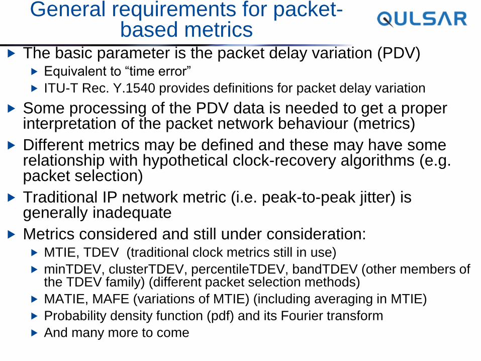
General requirements for packet-based metrics

The basic parameter is the packet delay variation (PDV) Equivalent to “time error”

ITU-T Rec. Y.1540 provides definitions for packet delay variation

Some processing of the PDV data is needed to get a proper interpretation of the packet network behaviour (metrics)

Different metrics may be defined and these may have some relationship with hypothetical clock-recovery algorithms (e.g. packet selection)

Traditional IP network metric (i.e. peak-to-peak jitter) is generally inadequate

Metrics considered and still under consideration: MTIE, TDEV (traditional clock metrics still in use)

minTDEV, clusterTDEV, percentileTDEV, bandTDEV (other members of the TDEV family) (different packet selection methods)

MATIE, MAFE (variations of MTIE) (including averaging in MTIE)

Probability density function (pdf) and its Fourier transform

And many more to come

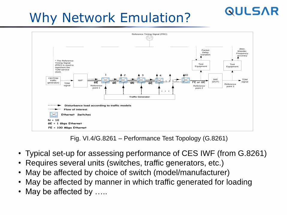
Why Network Emulation?

TDM

signal

Test

Equipment

CE(TDM

traffic

generator)

IWF

Test

Equipment

Packet

Delay

Variation

Jitter,

Wander,

Frequency

accuracy

TDM

signal

IWF

(DUT)

Reference

point 2

Reference

point 3

GE GE

1

GE = 1 Gbps Ethernet

FE = 100 Mbps Ethernet

GE FE or GEGE

Ethernet Switches

10

N = 10

. . .

Flow of interest

Disturbance load according to traffic models

GEGE GEGE

2

Traffic Generator

3 4

. . .

. . .

Reference Timing Signal (PRC)

* The Reference

Timing Signal

(PRC) is used to

represent the

TDM service

clock

Reference

point 1

Fig. VI.4/G.8261 – Performance Test Topology (G.8261)

• Typical set-up for assessing performance of CES IWF (from G.8261)

• Requires several units (switches, traffic generators, etc.)

• May be affected by choice of switch (model/manufacturer)

• May be affected by manner in which traffic generated for loading

• May be affected by …..

Packet Network Testing – a rational approach

Next generation test sets will emulate networks in terms of PDV (and packet loss profiles if necessary)

Pre-determined PDV profiles will allow repeatable and “deterministic” test results

Eliminates dependencies on manufacturer specific aspects of packet-switching network elements an method of introducing interfering traffic

Suitably chosen PDV profiles will permit standardization of performance requirements

PDV profiles can be created via simulation models, synthetic sequences as well as actual measurements

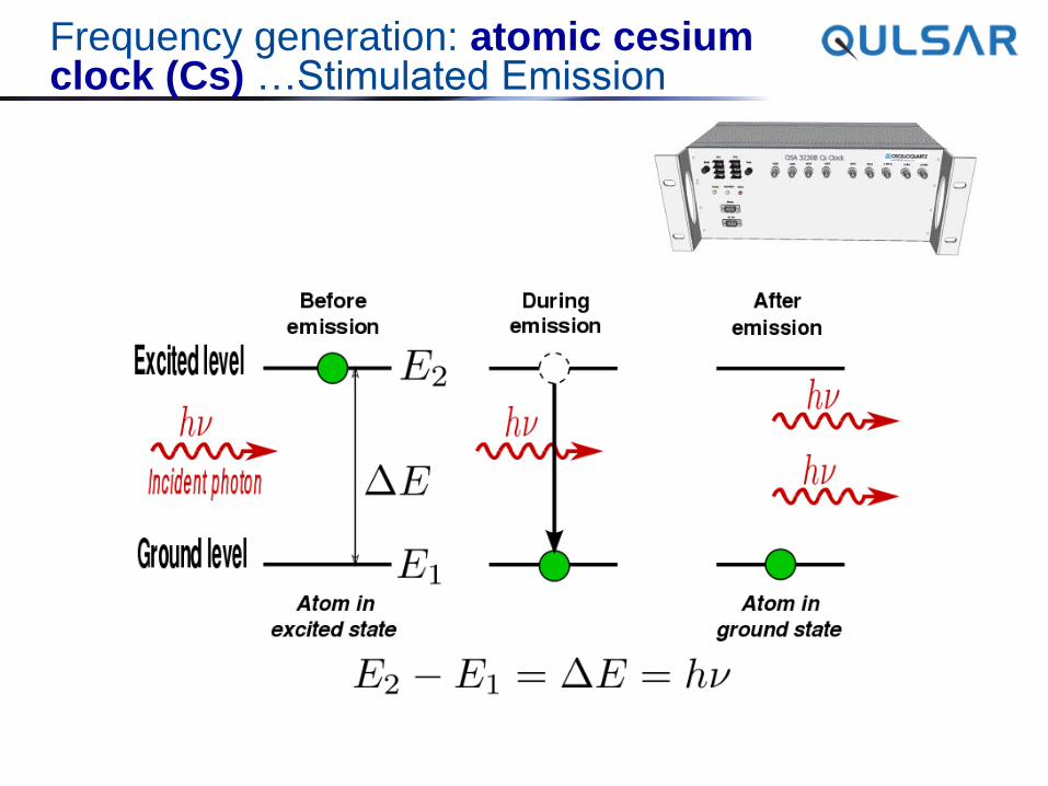
Frequency generation: atomic cesium clock (Cs) …Stimulated Emission

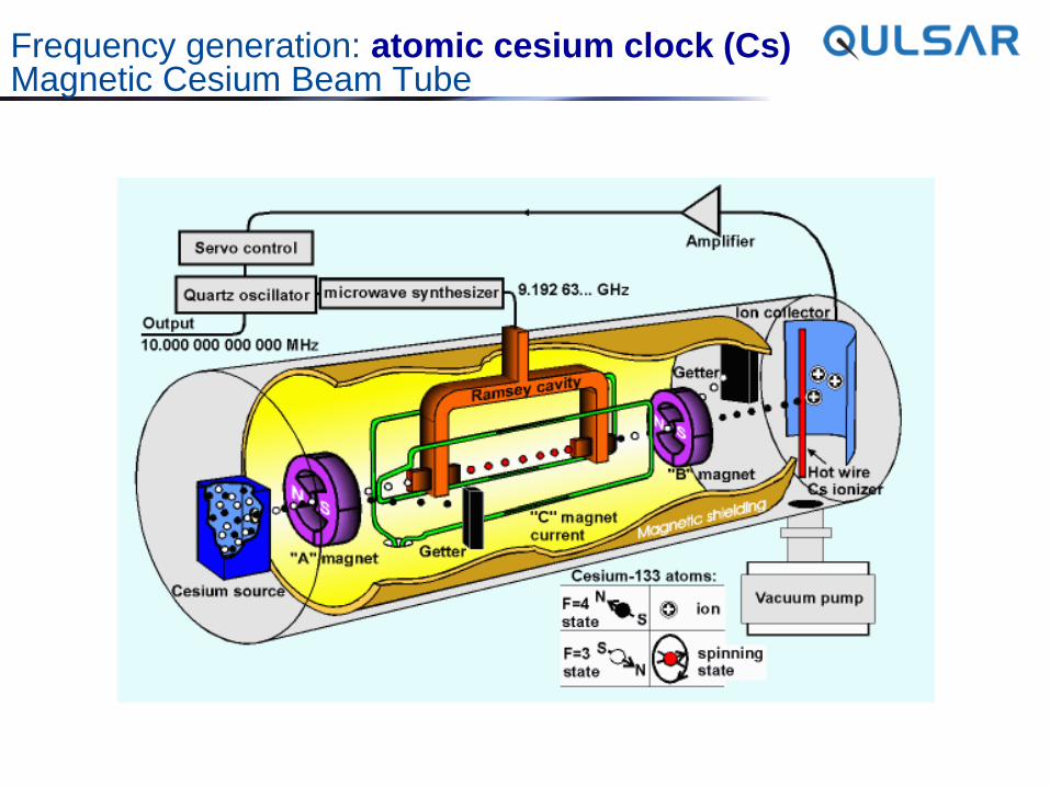
Frequency generation: atomic cesium clock (Cs) Magnetic Cesium Beam Tube

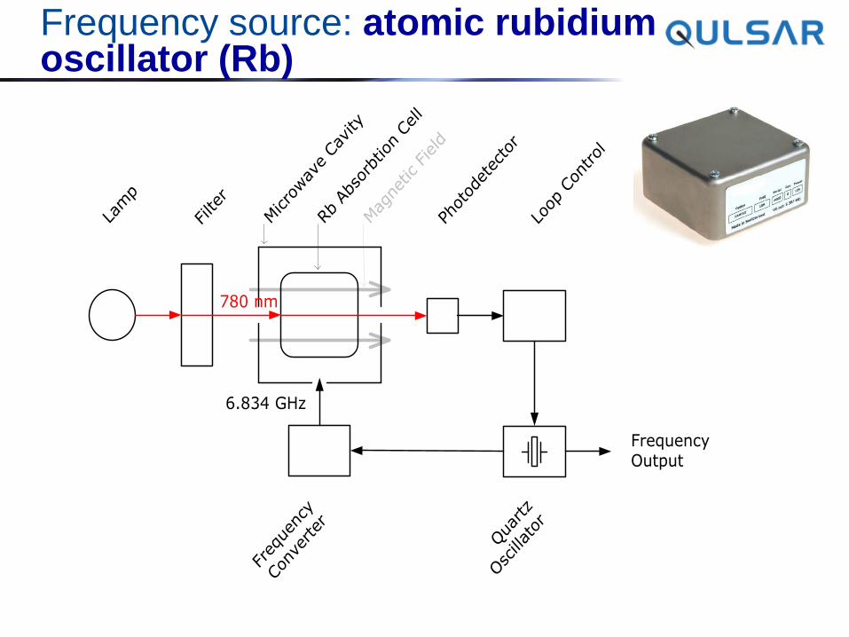
Frequency source: atomic rubidium oscillator (Rb)

Mag

netic Field

Photod

etec

tor

Loop

Con

trol

Lamp

Filter

Qua

rtz

Oscillator

Freq

uenc

y

Con

verter

Microwav

e Cav

ity

Rb Abs

orbtion Cell

Frequency Output

6.834 GHz

780 nm

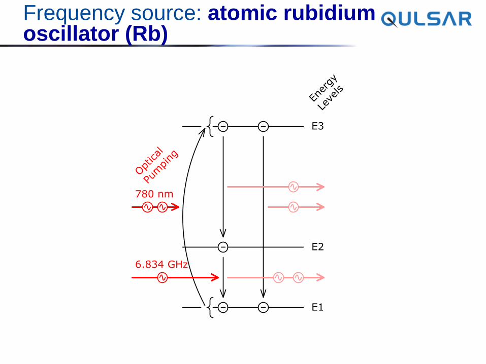
Frequency source: atomic rubidium oscillator (Rb)

E3

E2

E1

780 nm

6.834 GHz

Ener

gy

Leve

ls

Opt

ical

Pumping

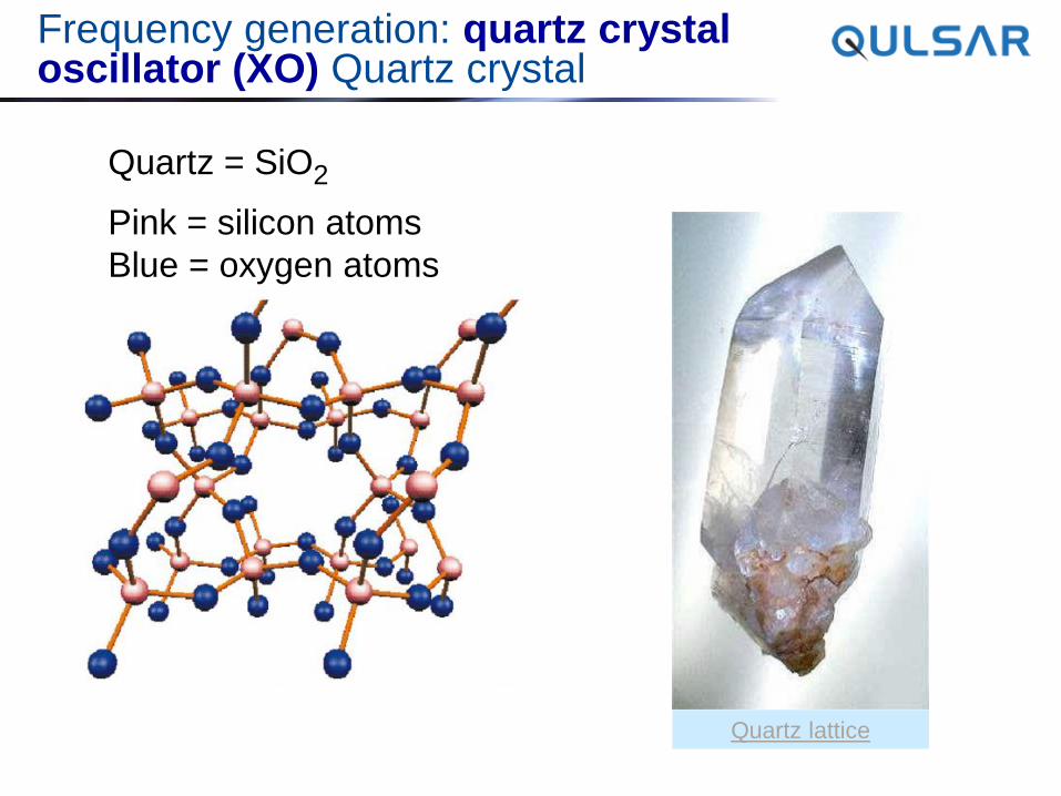
Frequency generation: quartz crystal oscillator (XO) Quartz crystal

Quartz = SiO2

Pink = silicon atoms

Blue = oxygen atoms

Quartz lattice

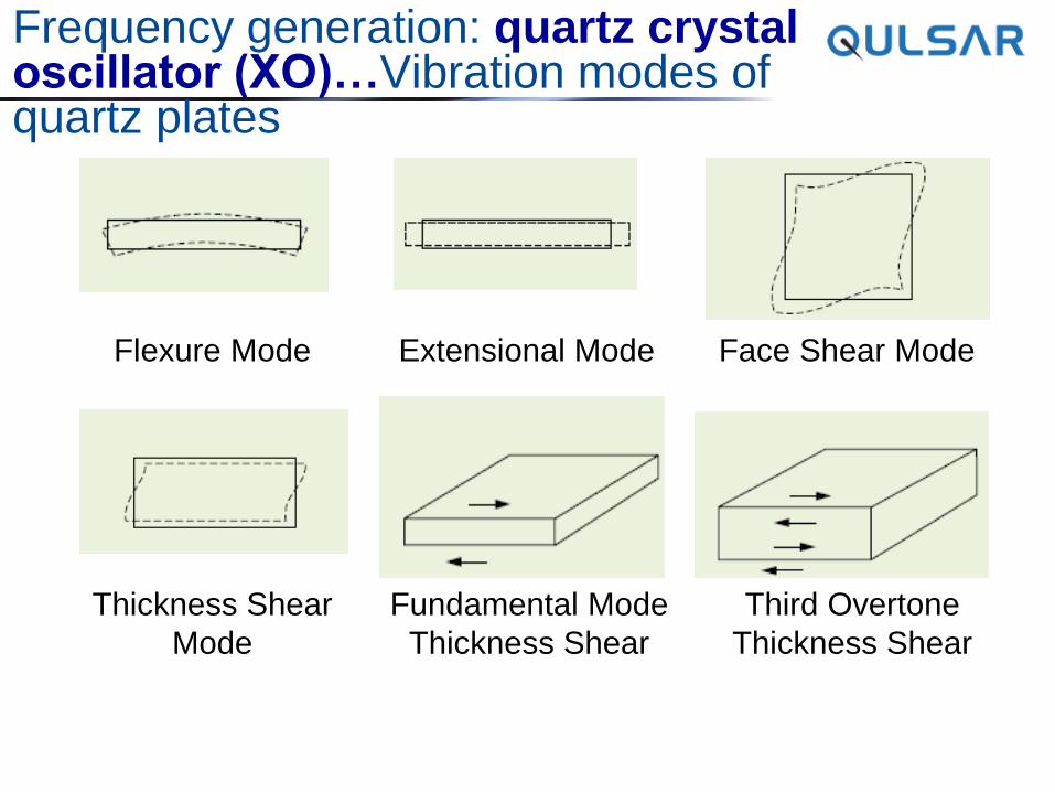
Frequency generation: quartz crystal oscillator (XO)…Vibration modes of quartz plates

Fundamental Mode

Thickness Shear

Third Overtone

Thickness Shear

Thickness Shear

Mode

Face Shear Mode Extensional Mode Flexure Mode

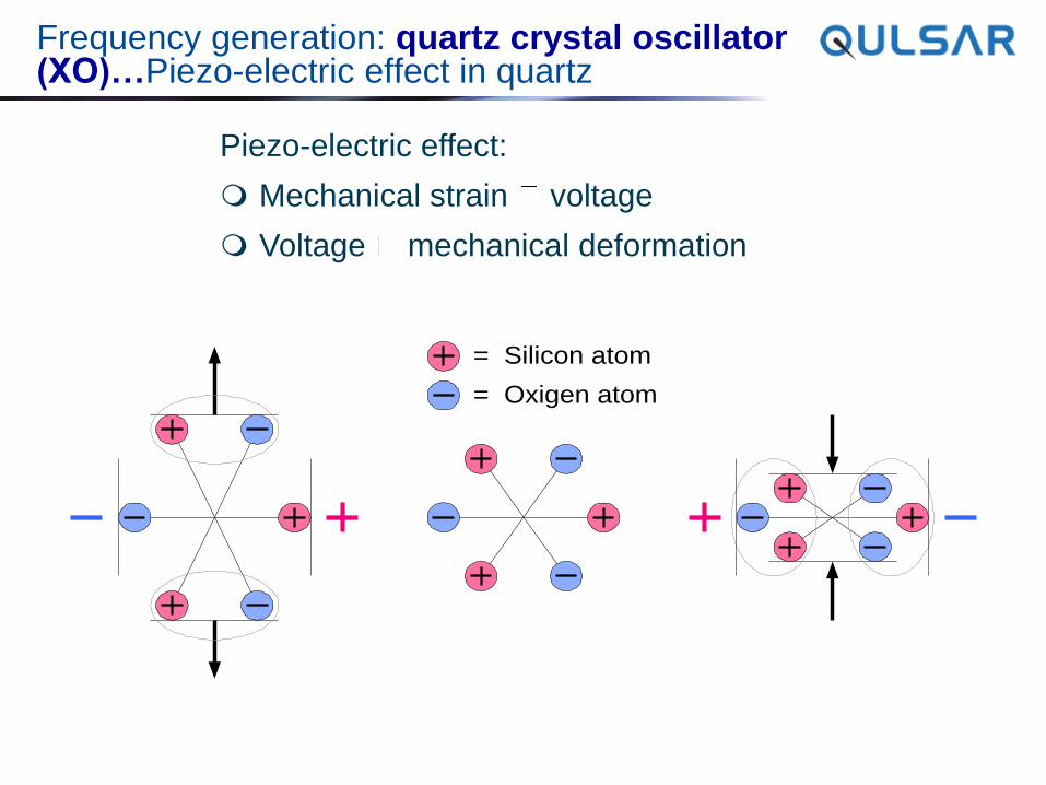
Frequency generation: quartz crystal oscillator (XO)…Piezo-electric effect in quartz

Piezo-electric effect:

Mechanical strain voltage

Voltage mechanical deformation

= Oxigen atom

= Silicon atom

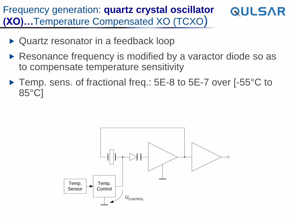
Frequency generation: quartz crystal oscillator

(XO)…Temperature Compensated XO (TCXO)

Quartz resonator in a feedback loop

Resonance frequency is modified by a varactor diode so as to compensate temperature sensitivity

Temp. sens. of fractional freq.: 5E-8 to 5E-7 over [-55°C to 85°C]

UCONTROL

Temp.

Control

Temp.

Sensor

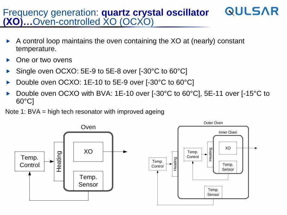
Frequency generation: quartz crystal oscillator (XO)…Oven-controlled XO (OCXO)

A control loop maintains the oven containing the XO at (nearly) constant temperature.

One or two ovens

Single oven OCXO: 5E-9 to 5E-8 over [-30°C to 60°C]

Double oven OCXO: 1E-10 to 5E-9 over [-30°C to 60°C]

Double oven OCXO with BVA: 1E-10 over [-30°C to 60°C], 5E-11 over [-15°C to 60°C]

Note 1: BVA = high tech resonator with improved ageing

XO

Temp.

Sensor

Temp.

Control

Heating

Oven

XO

Temp.

Sensor

Temp.

Control

Hea

ting

Temp.

Sensor

Hea

ting

Temp.

Control

Outer Oven

Inner Oven

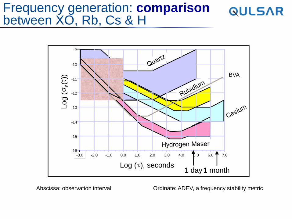
Frequency generation: comparison between XO, Rb, Cs & H

Log (

y (

t ))

Log ( t ), seconds

- 3.0 - 2.0 - 1.0 0.0 1.0 2.0 3.0 4.0 5.0 6.0 7.0

1 day 1 month

- 9

- 10

- 11

- 12

- 13

- 14

- 15

- 16

BVA

Abscissa: observation interval Ordinate: ADEV, a frequency stability metric

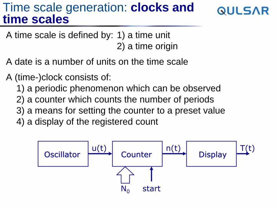
Oscillator Counter Display u(t) n(t) T(t)

start N0

Time scale generation: clocks and time scales

A time scale is defined by: 1) a time unit

2) a time origin

A date is a number of units on the time scale

A (time-)clock consists of:

1) a periodic phenomenon which can be observed

2) a counter which counts the number of periods

3) a means for setting the counter to a preset value

4) a display of the registered count

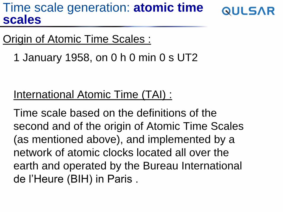
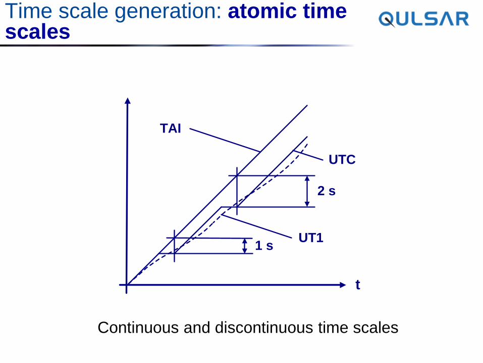
Time scale generation: atomic time scales

Origin of Atomic Time Scales :

1 January 1958, on 0 h 0 min 0 s UT2

International Atomic Time (TAI) :

Time scale based on the definitions of the

second and of the origin of Atomic Time Scales

(as mentioned above), and implemented by a

network of atomic clocks located all over the

earth and operated by the Bureau International

de l’Heure (BIH) in Paris .

1 s

2 s

t

TAI

UTC

UT1

Time scale generation: atomic time scales

Continuous and discontinuous time scales

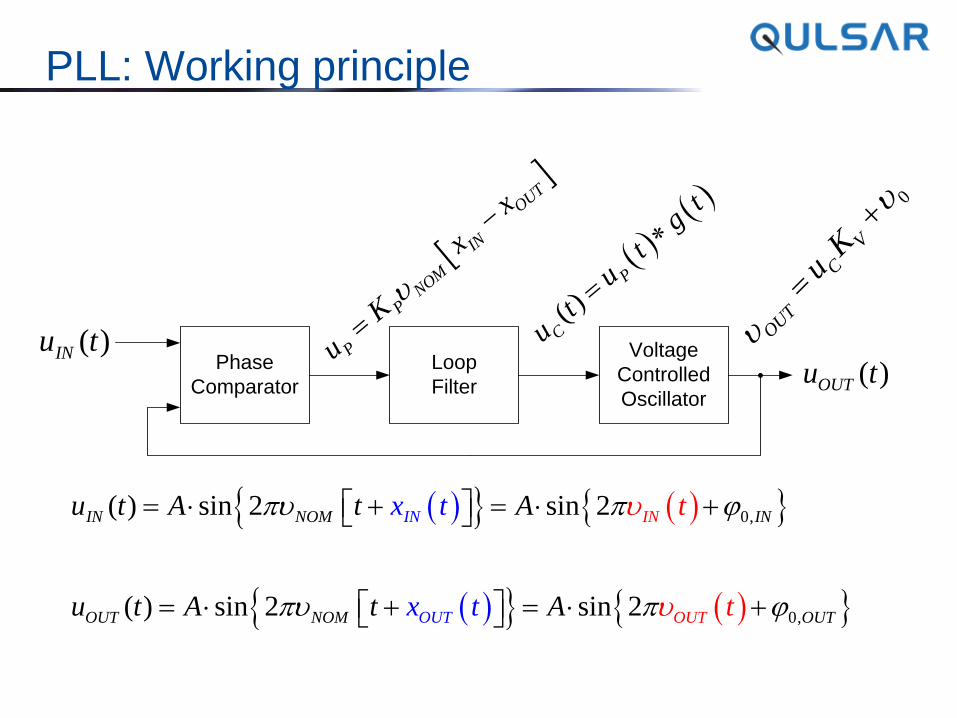
PLL: Working principle

Phase

Comparator

Loop

Filter

Voltage

Controlled

Oscillator

( )INu t( )OUTu t

0,

0,

( ) sin 2 sin 2

( ) sin 2 sin 2

IN NOM IN

OUT NOM

IN

OOU

IN

OT UT TU

u t A t A

u t A t A

t

t t

x

x

t

P

PNO

M

IN

OU

T

u

K

x

x

-

( )C

P

ut

ut

gt

0

OU

T

C

V

uK

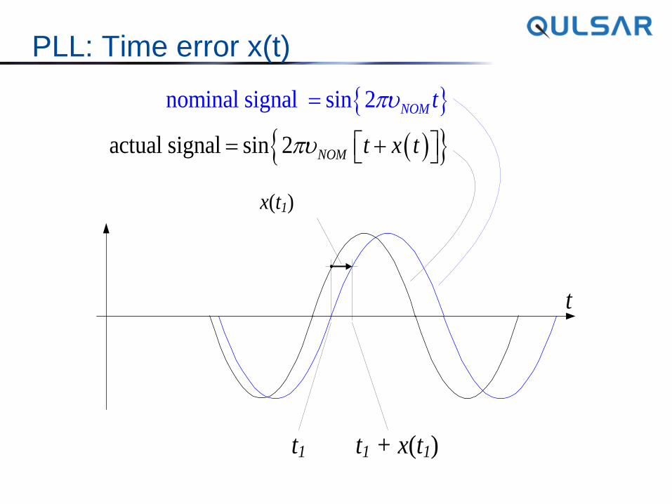
PLL: Time error x(t)

t1 t1 + x(t1)

nominal signal

actual signal

sin 2

sin 2

NO

NOM

M

t x t

t

x(t1)

t

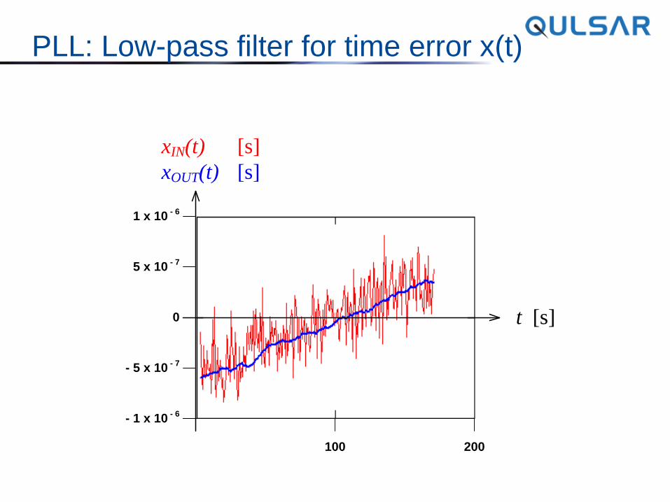
PLL: Low-pass filter for time error x(t)

0

100 200

t [s]

xIN(t) [s]

xOUT(t) [s]

1 x 10 - 6

5 x 10 - 7

- 5 x 10 - 7

- 1 x 10 - 6

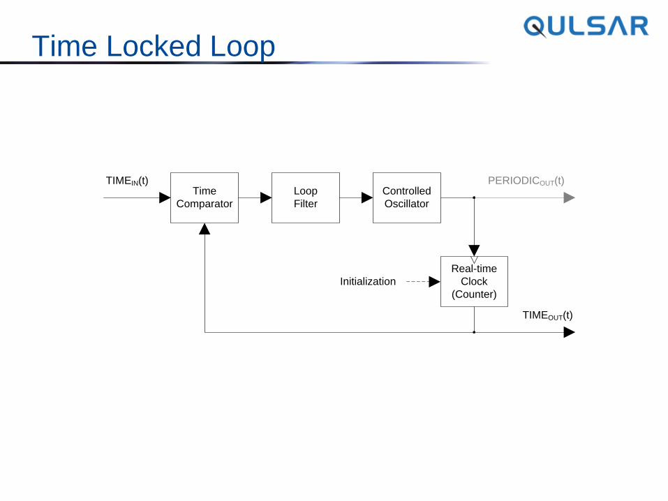
Time Locked Loop

Controlled

Oscillator

Time

Comparator

Loop

Filter

Real-time

Clock

(Counter)

Initialization

TIMEOUT(t)

TIMEIN(t) PERIODICOUT(t)