CHAPTER 5WATER DISTRIBUTION SYSTEMOPERATION: APPLICATION OFSIMULATED ANNEALING

Fred E. GoldmanKennedy/Jenks ConsultantsPhoenix, Arizona

Larry W. MaysDepartment of Civil and Environmental EngineeringArizona State University,Tempe, Arizona

5.1 INTRODUCTION

The operation of water distribution systems affects the water quality in these systems. EPA regulationsrequire that water quality be maintained at all points in the system including the point of delivery.Methods to optimize water system operations have been restricted to reducing costs related to pump-ing and costs related to sizing, construction, and/or maintenance of piping while meeting customerdemands, pressure limits, and tank operation restrictions. There have been few attempts to optimizewater system operations for both hydraulic and water quality performance and they have beenrestricted to simplified systems.

A new methodology that formulates the water distribution system problem as a discrete time optimalcontrol problem was developed that linked the method of simulated annealing with EPANET for opti-mal operation of water distribution systems for both water quality and hydraulic performance. Mostoptimization techniques require the calculation of derivatives, response functions, or other methodsthat are limited to specific problems. Simulated annealing allows optimization for a variety of objec-tive functions and can consider many modifications to operational conditions without reprogrammingof the optimization procedure. The new methodology was applied to two water systems as examples.The northwest pressure zone in the Austin, Texas application considered pump operation to mini-mize energy costs, which allowed comparison to published nonlinear optimization methods. The sec-ond system was the North Marin Water District, Novato, California system, which considered optimalpump operation for minimizing power costs while meeting hydraulic and water quality constraints. Acomparison is made between using a gradient-based method and simulated annealing.

Until 1974, government regulators and water system operators concentrated their efforts on meet-ing water quality Maximum Contaminant Levels (MCLs) at the water source or water treatmentplant. However, with the implementation of the Safe Water Drinking Act in 1974 and amendmentsin 1986 and 1996, water system operators are being required to meet standards throughout their dis-tribution systems and at the points of delivery. The Surface Water Drinking Rule requires that adetectable level of chlorine be maintained in the system. The Total Coliform Rule requires that totalcoliform standards be met at the customer’s tap. The Lead and Copper rule requires testing at thepoint of delivery (Clark, 1994b; Clark et al., 1994, 1995; Pontius, 1996).

Water quality can undergo significant changes as it travels through the water distribution system fromthe point of supply and/or treatment to the point of delivery. For example, chlorine concentration willdecrease with time in pipes and tanks through bulk decay and through reaction with the pipe wall. Also,chlorine mass leaves the system at demand nodes or can be added to the system at chlorine boosternodes. Mixing of water from different sources can also affect water quality (Clark et al., 1995).

5.1

Ch05_mays_144381-9 9/27/04 11:55 PM Page 5.1

Pumps are usually operated according to an operating policy, which includes the scheduling ofpump operation, which can affect water quality if the system pumps draw water from sources withdiffering water quality. Pump operation will affect the turnover rate of storage tanks. Chlorine dosagemay differ at each pump depending on the water source quality. For example, consider a pumpthat operates for 6 h divided into 1-h periods. The pump can either be on or off for any period. Thenumber of combinations is 26 � 64. A pump, which operates for 24 h divided into 1-h periods, has224 � 16,777,216 combinations. The 6-h example can be solved by trial and error but the 24-h exampleis prohibitively large to solve by trial and error. For large combinatorial optimization problems, sim-ulated annealing provides a manageable solution strategy.

These considerations have generated a need for computer models and optimization techniquesthat consider water quality in the water distribution system as well as system hydraulics.

5.2 GENERAL PROBLEM STATEMENT

Consider a water distribution system with M pipes, K junction nodes, S storage nodes (tanks or reser-voirs), and P pumps, which are operated for T time periods. The objective function is the minimiza-tion of the total energy cost for pumping:

Minimize Z � �P

p � 1 �T

t � 1

Dpt (5.1)

where UCt � unit energy cost of pumping during time period t ($/kw-hr)PPpt � power of pump during time period t (hp)Dpt � length of time pump p operates during time period t (hr)

EFFpt � efficiency of pump p during period t.

Conservation of mass and conservation of energy conditions must be met throughout the waterdistribution system. These conditions make up the system hydraulic constraints. For each link (whichcan be a pipe or pump) between nodes i and j and node k, the conservation of mass is

�i

(qik)t � �j

(qkj)t � Qkt � 0 ∀i, j � M; k � 1,…,K and t � 1,…,T (5.2)

where qik � flow in link connecting nodes i and k during time period t and Qkt � flow consumed (�)or supplied (�) at node k during time period t. The conservation of energy for each pipe connectingnodes i and j, in the set of all pipes M is:

hit � hjt � f �qij�t ∀i, j � M and t � 1,…,T (5.3)

where hit � hydraulic grade line elevation (ground elevation and pressure head) at node i during timet and f(qij)t � headloss in link connecting nodes i and j during time t. The total number of hydraulicconstraints is (K � M)T, and the total number of unknowns is also (K � M)T, which are the dis-charges in M pipes and the hydraulic grade line elevations at K nodes.

In addition to the equality hydraulic constraints there are inequality hydraulic bound constraints.The nodal pressure head bounds are

Hkt � Hkt � H�kt k � 1,…,K and t � 1,…,T (5.4)

where Hkt and Hkt are, respectively, the lower and upper bounds on the pressure head at node k at time t.The pump operation problem is an extended period simulation. The height of water stored at a

tank for the current time period t, yst, is a function of the height of water stored from the previoustime period and the flow entering or leaving the tank during the period �t and can be expressed as

yst � ys(t�1) � �t (5.5)qs(t�1)�As

UCt 0.746 PPpt��EFFpt

5.2 CHAPTER FIVE

Ch05_mays_144381-9 9/27/04 11:55 PM Page 5.2

where As � cross sectional area of tank s and qs � flow entering or leaving the tank during periodst and t � 1. The inequality bound constraints on the height of water in the storage tanks are

y�st � yst � y�st s � 1,…,S and t � 1,…,T (5.6)

where y�st and y�st are, respectively, the lower and upper bound tank water levels.

The water quality constraint is the conservation of mass of the chemical in each pipe m connect-ing nodes i and j in the set of all pipes M and is

� � � (Cij)t ∀i, j � M and t � 1,…,T (5.7)

where (Cij)t � concentration of chemical in pipe m connecting nodes i and j as a function of dis-tance and time (mass/ft3)

xij � distance along pipe (ft)Aij � cross-sectional area of pipe connecting nodes i and j

(Cij)t � rate of reaction of chemical within pipe connecting nodes i and j at time t(mass/ft3/day).

The bounds on chemical concentrations are

Cnt � Cnt � C�nt n � 1,…,N and t � 1,…,T (5.8)

where Cnt and C�nt are, respectively, the lower and upper bounds of the chemical concentration.The above formulation results in a large-scale nonlinear programming problem with decision

variables (qij)t, Hkt, yst, Dpt, and (Cij)t. In the proposed solution methodology, the decision variablesare partitioned into two sets: control (independent) and state (dependent) variables. The operation ofa pump during a time period (on or off) is the control variable. The problem is formulated above asa discrete-time optimal control problem.

5.3 SOLUTION METHODOLOGY

5.3.1 Previous Models for Water Distribution System Optimization

Ormsbee and Lansey (1994) reviewed methods used to optimize the operation of water supply pump-ing systems to minimize operation costs. Ostfeld and Shamir (1993) developed a water quality opti-mization model that optimized pumping costs and water quality using steady-state and dynamicconditions using GAMS/MINOS [general algebraic modeling system (Brooke et al., 1988); mathe-matical in-core nonlinear optimization systems (Murtagh and Saunders, 1982)]. Ormsbee (1991)suggested that on–off operation of pumps poses a difficulty for optimization techniques that requirecontinuous functions. Computer-based water quality models exhibit the same difficulties. Most mod-eling methods include numerical methods rather than continuous functions. Linear superpositionwas used by Boccelli et al. (1998) for the optimal scheduling of booster disinfection stations bydeveloping system-dependent discretized impulse response coefficients using EPANET and linkingwith the LP solver MINOS (Murtagh and Saunders, 1987).

Dynamic programming has been used for the optimal scheduling of pumps in a water distributionsystem by Coulbeck and Orr (1982) and Coulbeck et al. (1987). The method is sensitive to the numberof reservoir states and the number of pumps. In general, the increase in number of discretizations andstate variables increases the size of the problem dramatically, which is known as the curse of dimen-sionality (Mays and Tung, 1992). This has restricted the application of this method to small systems.

The nonlinear programming approach by Brion and Mays (1991) evaluates gradients using finitedifferences or a mathematical approach to provide derivatives required by GRG2, which solves non-linear optimization problems by using the generalized reduced gradient method (Lasdon et al.,

∂(Cij)j�∂xij

(qij)t�Aij

∂(Cij)t�

∂t

WATER DISTRIBUTION SYSTEM OPERATION: SIMULATED ANNEALING 5.3

Ch05_mays_144381-9 9/27/04 11:55 PM Page 5.3

1978). The method has been used for scheduling pump operations to minimize energy and improvewater quality by Sakarya (1998) and Sakarya and Mays (2000), who considered three objective func-tions: (1) the minimization of the deviations of actual concentrations from a desired concentration,(2) minimization of total pump duration times, and (3) the minimization of total energy while meet-ing water quality constraints.

5.3.2 The Method of Simulated Annealing

Simulated annealing is a combinatorial optimization method that uses the Metropolis algorithm toevaluate the acceptability of alternate arrangements and slowly converge to an optimum solution.The method does not require derivatives and has the flexibility to consider many different objectivefunctions and constraints. Simulated annealing uses concepts from statistical thermodynamics andapplies them to combinatorial optimization problems. Kirkpatrick et al. (1983) explain how theMetropolis algorithm was developed to provide the simulation of a system of atoms at a high tem-perature that slowly cools to its ground energy state. If an atom is given a small random change therewill be a change in system energy �E. If �E � 0, the new configuration is accepted. If �E 0, thenthe decision to change the system configuration is treated probabilistically. The probability that thenew system is accepted is calculated by:

P(�E) � exp(��E / kB T) (5.9)

A random number evenly distributed between 0 and 1 is chosen. If the number is smaller than P(�E)then the new configuration is accepted; otherwise it is discarded and the old configuration is used togenerate the next arrangement. The Metropolis algorithm simulates the random movement of atomsin a water bath at temperature T. By using Eq. (5.9), the system becomes a Boltzmann distribution.

Entropy is a measure of the variation of energy at a given temperature. At higher temperaturesthere is significant energy variation, which reduces dramatically as the temperatures are lowered.This implies that the annealing process should not get “stuck” because transitions out of an energystate are always possible. Also, the process is a form of adaptive divide-and-conquer. Gross featuresof the eventual solution appear at the higher temperatures with fine details developing at low tem-peratures (Kirkpatrick et al., 1983).

The requirements for applying simulated annealing to an engineering problem are: (1) a conciserepresentation of the configuration of the decision variables, (2) a scalar cost function, (3) a proce-dure for generating rearrangements of the system, (4) a control parameter (T) and an annealingschedule, and (5) a criterion for termination. (Dougherty and Marryott, 1991).

5.3.3 Configuration of Decision Variables

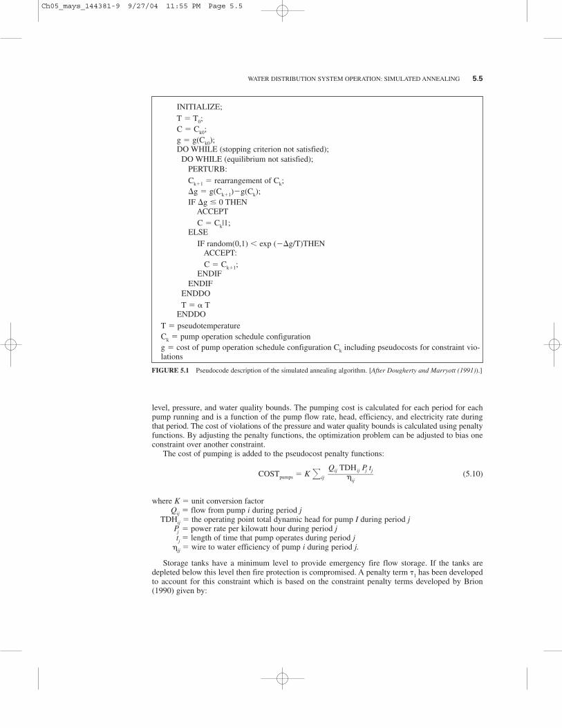
The decision variables consist of the operational schedule of each pump during discrete time periods.For this application, the 24-h day was divided into 1-h periods. The program finds the optimumpump schedule where each of the pumps is either on or off during each of the time periods. A con-figuration is a given schedule of pump operation, which determines in which 1-h period each pumpis operating. EPANET is then run using that pump configuration. The program results are used torate the performance of the simulation. The decision on whether to retain or change the pump operationconfiguration is based on the Metropolis algorithm as shown in Fig. 5.1, a pseudocode descriptionof the adaptation of the simulated annealing algorithm to pump operation optimization.

5.3.4 Development of Cost Function

The cost function g(Ci) for a given configuration Ci is used in place of energy of a system of atoms. Thetemperature T can be considered a control parameter, which has the same units as the cost function.The cost function should include the cost of pumping and penalties for violations of the storage tank

5.4 CHAPTER FIVE

Ch05_mays_144381-9 9/27/04 11:55 PM Page 5.4

level, pressure, and water quality bounds. The pumping cost is calculated for each period for eachpump running and is a function of the pump flow rate, head, efficiency, and electricity rate duringthat period. The cost of violations of the pressure and water quality bounds is calculated using penaltyfunctions. By adjusting the penalty functions, the optimization problem can be adjusted to bias oneconstraint over another constraint.

The cost of pumping is added to the pseudocost penalty functions:

COSTpumps � K �ij (5.10)

where K � unit conversion factorQij � flow from pump i during period j

TDHij � the operating point total dynamic head for pump I during period jPj � power rate per kilowatt hour during period jtj � length of time that pump operates during period j

�jj � wire to water efficiency of pump i during period j.

Storage tanks have a minimum level to provide emergency fire flow storage. If the tanks aredepleted below this level then fire protection is compromised. A penalty term �1 has been developedto account for this constraint which is based on the constraint penalty terms developed by Brion(1990) given by:

Qij TDHij Pj tj���ij

WATER DISTRIBUTION SYSTEM OPERATION: SIMULATED ANNEALING 5.5

INITIALIZE;T � T0;C � Ck0;g � g(Ck0);DO WHILE (stopping criterion not satisfied);

DO WHILE (equilibrium not satisfied);PERTURB:Ck�1 � rearrangement of Ck;�g � g(Ck�1)�g(Ck);IF �g � 0 THEN

ACCEPTC � Ck|1;

ELSEIF random(0,1) exp (��g/T)THEN

ACCEPT:C � Ck�1;

ENDIFENDIF

ENDDOT � � T

ENDDOT � pseudotemperatureCk � pump operation schedule configurationg � cost of pump operation schedule configuration Ck including pseudocosts for constraint vio-lations

FIGURE 5.1 Pseudocode description of the simulated annealing algorithm. [After Dougherty and Marryott (1991)).]

Ch05_mays_144381-9 9/27/04 11:55 PM Page 5.5

�1 � �j �s (min [0, Esj � Emin,s])2 (5.11)

where �1 � penalty for violations of the tank low water level boundEsj � water level for tank s during period j

Emin,s � lower bound or the minimum level in tank s�s � penalty term for tank low-level constraint for tanks

Cohen (1982) has stated “optimization of a network over a limited horizon of, say, 24 hours hasno meaning without the requirement of some periodicity in operation; a simple way to do that is toconstrain the final states to be the same as the initial ones.” A constraint �2 is developed to generatea cost if the tank levels do not return to their starting elevation.

�2 � �s �s2 (min [0, 1 � / Es,1 � Esj / ])2 (5.12)

where Es,1 � water level for tank s at beginning of the simulation, during period 1Es,j � water level for tank s at the end of the simulation, during the final period j�s2 � penalty term for beginning and ending tank level constraint for tank s

For a 24-h simulation the concept of returning tanks to their starting level is somewhat addressedby using a starting configuration where the pumps supply a volume of water equal to the sum of thenodal demands. Providing a total volume of pumped water equal to the total volume of the systemdemands will return the tanks exactly to their original level if there is only one tank. Even if pump-ing equals demand exactly, the tanks may not return to their original level if there are several tanksunless the tanks all start full; because one tank may supply water to another tank during the simula-tion, the total volume stored will be the same but shifted from one tank to another.

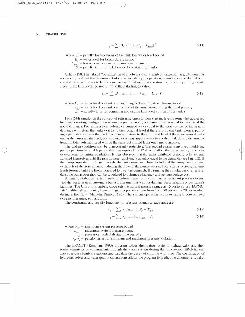
The Cohen condition may be unnecessarily restrictive. The second example involved modifyingpump operation for a 24-h period that was repeated for 12 days to allow the water quality variationsto overcome the initial conditions. It was observed that the tanks exhibited periodic behavior andadjusted themselves until the pumps were supplying a quantity equal to the demands (see Fig. 5.2). Ifthe pumps operated for longer periods, the tanks remained closer to full and the pump heads movedto the left of the system curve reducing the flow. If the pumps operated for shorter periods, the tanklevels lowered until the flows increased to meet the demands. By running the simulations over severaldays, the pump operation can be scheduled to optimize efficiency and perhaps reduce cost.

A water distribution system needs to deliver water to its customers at sufficient pressure to ser-vice the water system customers but at a pressure that will not damage water systems or customer’sfacilities. The Uniform Plumbing Code sets the normal pressure range as 15 psi to 80 psi (IAPMO,1994), although a city may have a range in a pressure zone from 40 to 80 psi with a 20 psi residualduring a fire flow (Malcolm Pirnie, 1996). The system operation needs to operate between twoextreme pressures, pmin and pmax.

The constraints and penalty functions for pressure bounds at each node are:

�3 � �kj �1 (min [0, Pkj � Pmin]2 (5.13)

�4 � �kj �2 (min [0, Pmax � Pkj]2 (5.14)

where pmin � minimum system pressure boundpmax � maximum system pressure bound

pkj � pressure at node k during time period j�1, �2 � penalty terms for minimum and maximum pressure violations

The EPANET (Rossman, 1993) program solves distribution systems hydraulically and thenroutes chemicals or contaminants through the water system during the time period. EPANET canalso consider chemical reactions and calculate the decay of chlorine with time. The combination ofhydraulic solver and water quality calculations allows the program to predict the chlorine residual at

5.6 CHAPTER FIVE

Ch05_mays_144381-9 9/27/04 11:55 PM Page 5.6

any node in the system at any time period. A penalty term will be used to consider upper and lowerlimit bounds on free chlorine to adjust the cost function for chlorine violations.

The penalty terms for minimum and maximum free chlorine concentration are:

�5 � �kj �3 (min [0, ckj � cmin])n (5.15)

�6 � �kj �4 (min [0, cmax � ckj])n (5.16)

where cmin � minimum free chlorine concentrationcmax � maximum free chlorine concentration

ckj � chlorine residual concentration at node k during time period j�3 � penalty term for minimum chlorine residual pressure bound violations�4 � penalty term for maximum chlorine residual pressure bound violations

The value of n will usually be 2. In cases where the lower concentration bound is more important, avalue of n 1 will place a higher penalty on minimum free chlorine violations. There will also bea term for the amount of chlorine used. The goal will be to meet the chlorine residual bounds whileusing the smallest amount of chlorine. Not only will the operational cost be decreased but also thecreation of Total Trihalomethane (TTHM) will also be reduced.

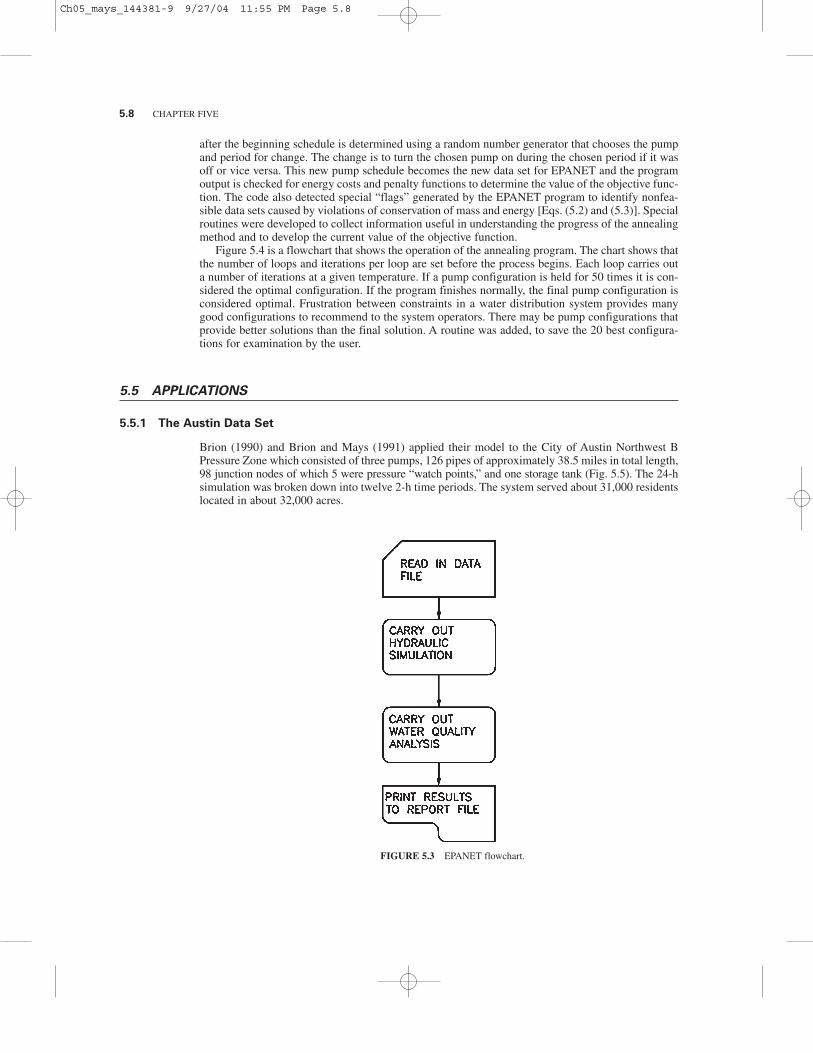
5.4 DEVELOPMENT OF SOFTWARE

Version 1.1e of EPANET (5/1/96) authored by Dr. Lewis A. Rossman, Risk Reduction EngineeringLaboratory of the Office of Research and Development, U.S.E.P.A., Cincinnati, Ohio, was used asthe basis of the annealing computer program. The program source files, in the C language, were pro-vided by Dr. Rossman. The basic strategy was to use EPANET as the simulator and to developaround EPANET new functions that calculate penalties or costs, generate pump operation configu-rations, and evaluate the acceptance of potential configurations using the Metropolis algorithm. TheEPANET program was developed for a single simulation as described by the flowchart in Fig. 5.3.In order to carry out the numerous simulations required for annealing, several modifications wererequired. New functions were written in the C programming language to carry out penalty calcula-tions, generate pump operation configurations, modify the temperature according to the annealingschedule, and analyze each result using the Metropolis algorithm. Pump scheduling is determined bydividing the 24-h day into 1- or 2-h periods. The pump schedule is repeated if the simulation is car-ried out for several days. The schedule specifies the on–off condition for each pump for each period.The starting pump operation configuration is completely arbitrary. Each pump operation schedule

WATER DISTRIBUTION SYSTEM OPERATION: SIMULATED ANNEALING 5.7

FIGURE 5.2 Periodic behavior.

Ch05_mays_144381-9 9/27/04 11:55 PM Page 5.7

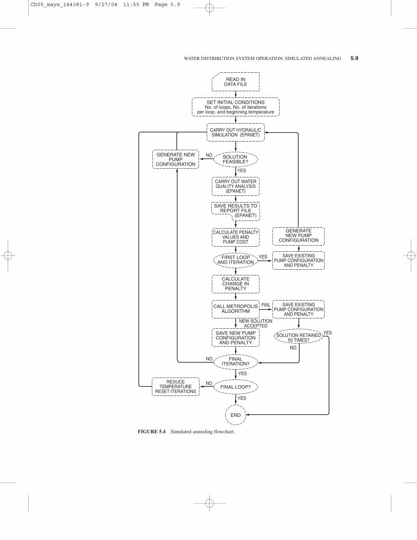
after the beginning schedule is determined using a random number generator that chooses the pumpand period for change. The change is to turn the chosen pump on during the chosen period if it wasoff or vice versa. This new pump schedule becomes the new data set for EPANET and the programoutput is checked for energy costs and penalty functions to determine the value of the objective func-tion. The code also detected special “flags” generated by the EPANET program to identify nonfea-sible data sets caused by violations of conservation of mass and energy [Eqs. (5.2) and (5.3)]. Specialroutines were developed to collect information useful in understanding the progress of the annealingmethod and to develop the current value of the objective function.

Figure 5.4 is a flowchart that shows the operation of the annealing program. The chart shows thatthe number of loops and iterations per loop are set before the process begins. Each loop carries outa number of iterations at a given temperature. If a pump configuration is held for 50 times it is con-sidered the optimal configuration. If the program finishes normally, the final pump configuration isconsidered optimal. Frustration between constraints in a water distribution system provides manygood configurations to recommend to the system operators. There may be pump configurations thatprovide better solutions than the final solution. A routine was added, to save the 20 best configura-tions for examination by the user.

5.5 APPLICATIONS

5.5.1 The Austin Data Set

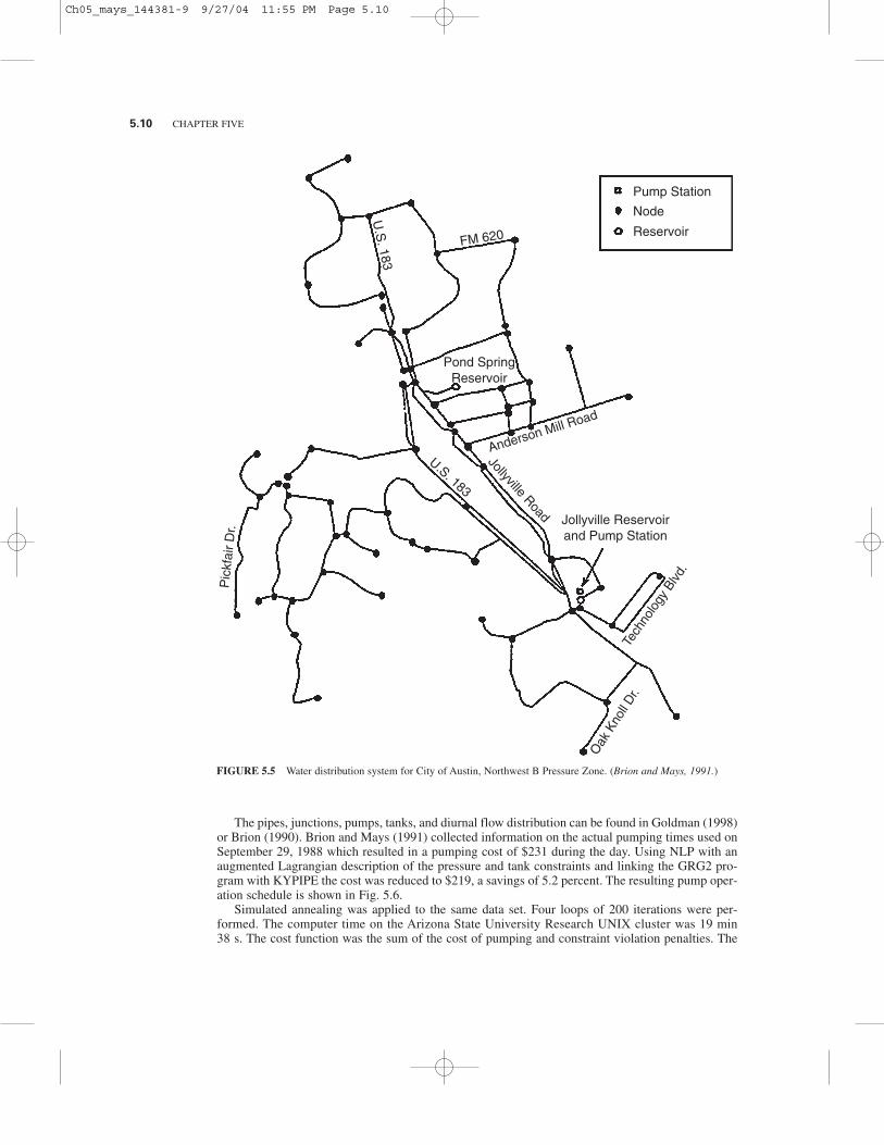
Brion (1990) and Brion and Mays (1991) applied their model to the City of Austin Northwest BPressure Zone which consisted of three pumps, 126 pipes of approximately 38.5 miles in total length,98 junction nodes of which 5 were pressure “watch points,” and one storage tank (Fig. 5.5). The 24-hsimulation was broken down into twelve 2-h time periods. The system served about 31,000 residentslocated in about 32,000 acres.

5.8 CHAPTER FIVE

FIGURE 5.3 EPANET flowchart.

Ch05_mays_144381-9 9/27/04 11:55 PM Page 5.8

WATER DISTRIBUTION SYSTEM OPERATION: SIMULATED ANNEALING 5.9

READ INDATA FILE

SET INITIAL CONDITIONSNo. of loops, No. of iterations

per loop, and beginning temperature

CARRY OUT HYDRAULICSIMULATION (EPANET)

GENERATE NEWPUMP

CONFIGURATION

SOLUTIONFEASIBLE?

CARRY OUT WATERQUALITY ANALYSIS

(EPANET)

SAVE RESULTS TOREPORT FILE

(EPANET)

CALCULATE PENALTYVALUES ANDPUMP COST

GENERATENEW PUMP

CONFIGURATION

FIRST LOOPAND ITERATION

SAVE EXISTINGPUMP CONFIGURATION

AND PENALTY

SAVE EXISTINGPUMP CONFIGURATION

AND PENALTY

CALCULATECHANGE INPENALTY

CALL METROPOLISALGORITHM

SAVE NEW PUMPCONFIGURATION

AND PENALTY

SOLUTION RETAINED50 TIMES?

FINALITERATION?

FINAL LOOP?REDUCE

TEMPERATURERESET ITERATIONS

END

NO

YES

YES

YES

YES

YES

NO

NO

NO

FAIL

NEW SOLUTIONACCEPTED

FIGURE 5.4 Simulated annealing flowchart.

Ch05_mays_144381-9 9/27/04 11:55 PM Page 5.9

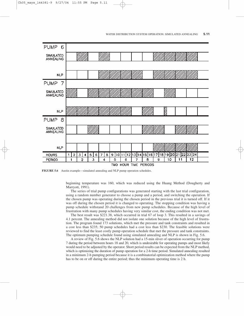
The pipes, junctions, pumps, tanks, and diurnal flow distribution can be found in Goldman (1998)or Brion (1990). Brion and Mays (1991) collected information on the actual pumping times used onSeptember 29, 1988 which resulted in a pumping cost of $231 during the day. Using NLP with anaugmented Lagrangian description of the pressure and tank constraints and linking the GRG2 pro-gram with KYPIPE the cost was reduced to $219, a savings of 5.2 percent. The resulting pump oper-ation schedule is shown in Fig. 5.6.

Simulated annealing was applied to the same data set. Four loops of 200 iterations were per-formed. The computer time on the Arizona State University Research UNIX cluster was 19 min38 s. The cost function was the sum of the cost of pumping and constraint violation penalties. The

5.10 CHAPTER FIVE

Pump Station

Node

ReservoirFM 620

U.S

. 183

Pond SpringReservoir

Anderson Mill Road

Jollyville Road

U.S. 183

Tech

nolo

gy B

lvd.

Jollyville Reservoirand Pump Station

Oak

Kno

ll D

r.

Pic

kfai

r D

r.

FIGURE 5.5 Water distribution system for City of Austin, Northwest B Pressure Zone. (Brion and Mays, 1991.)

Ch05_mays_144381-9 9/27/04 11:55 PM Page 5.10

beginning temperature was 160, which was reduced using the Huang Method (Dougherty andMarryott, 1991).

The series of trial pump configurations was generated starting with the last trial configuration,using a random number generator to choose a pump and a period, and switching the operation. Ifthe chosen pump was operating during the chosen period in the previous trial it is turned off. If itwas off during the chosen period it is changed to operating. The stopping condition was having apump schedule withstand 20 challenges from new pump schedules. Because of the high level offrustration with many pump schedules having very similar cost, the ending condition was not met.

The best result was $221.38, which occurred in trial 67 of loop 3. This resulted in a savings of4.1 percent. The annealing method did not isolate one solution because of the high level of frustra-tion. The program found 173 solutions, which met the pressure and tank constraints and resulted ina cost less than $235; 50 pump schedules had a cost less than $230. The feasible solutions werereviewed to find the least costly pump operation schedule that met the pressure and tank constraints.The optimum pumping schedule found using simulated annealing and NLP is shown in Fig. 5.6.

A review of Fig. 5.6 shows the NLP solution had a 15-min sliver of operation occurring for pump7 during the period between hours 18 and 20, which is undesirable for operating pumps and most likelywould need to be adjusted by the operator. Short period results can be expected from the NLP method,which is optimizing the duration of pump operation for a 2-h time period. Simulated annealing resultedin a minimum 2-h pumping period because it is a combinatorial optimization method where the pumphas to be on or off during the entire period; thus the minimum operating time is 2 h.

WATER DISTRIBUTION SYSTEM OPERATION: SIMULATED ANNEALING 5.11

FIGURE 5.6 Austin example—simulated annealing and NLP pump operation schedules.

Ch05_mays_144381-9 9/27/04 11:55 PM Page 5.11

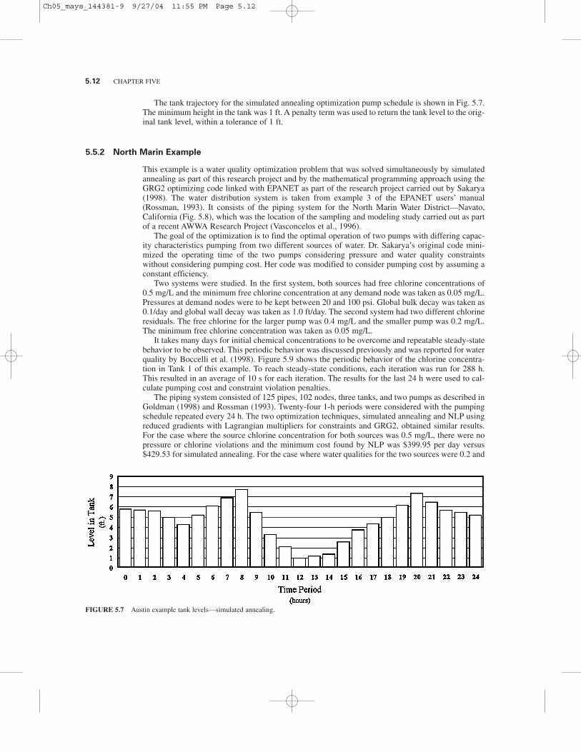
The tank trajectory for the simulated annealing optimization pump schedule is shown in Fig. 5.7.The minimum height in the tank was 1 ft. A penalty term was used to return the tank level to the orig-inal tank level, within a tolerance of 1 ft.

5.5.2 North Marin Example

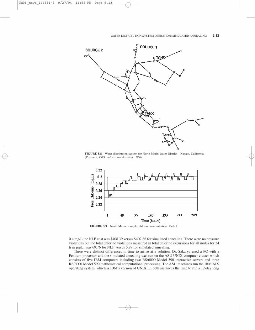
This example is a water quality optimization problem that was solved simultaneously by simulatedannealing as part of this research project and by the mathematical programming approach using theGRG2 optimizing code linked with EPANET as part of the research project carried out by Sakarya(1998). The water distribution system is taken from example 3 of the EPANET users’ manual(Rossman, 1993). It consists of the piping system for the North Marin Water District—Navato,California (Fig. 5.8), which was the location of the sampling and modeling study carried out as partof a recent AWWA Research Project (Vasconcelos et al., 1996).

The goal of the optimization is to find the optimal operation of two pumps with differing capac-ity characteristics pumping from two different sources of water. Dr. Sakarya’s original code mini-mized the operating time of the two pumps considering pressure and water quality constraintswithout considering pumping cost. Her code was modified to consider pumping cost by assuming aconstant efficiency.

Two systems were studied. In the first system, both sources had free chlorine concentrations of0.5 mg/L and the minimum free chlorine concentration at any demand node was taken as 0.05 mg/L.Pressures at demand nodes were to be kept between 20 and 100 psi. Global bulk decay was taken as0.1/day and global wall decay was taken as 1.0 ft/day. The second system had two different chlorineresiduals. The free chlorine for the larger pump was 0.4 mg/L and the smaller pump was 0.2 mg/L.The minimum free chlorine concentration was taken as 0.05 mg/L.

It takes many days for initial chemical concentrations to be overcome and repeatable steady-statebehavior to be observed. This periodic behavior was discussed previously and was reported for waterquality by Boccelli et al. (1998). Figure 5.9 shows the periodic behavior of the chlorine concentra-tion in Tank 1 of this example. To reach steady-state conditions, each iteration was run for 288 h.This resulted in an average of 10 s for each iteration. The results for the last 24 h were used to cal-culate pumping cost and constraint violation penalties.

The piping system consisted of 125 pipes, 102 nodes, three tanks, and two pumps as described inGoldman (1998) and Rossman (1993). Twenty-four 1-h periods were considered with the pumpingschedule repeated every 24 h. The two optimization techniques, simulated annealing and NLP usingreduced gradients with Lagrangian multipliers for constraints and GRG2, obtained similar results.For the case where the source chlorine concentration for both sources was 0.5 mg/L, there were nopressure or chlorine violations and the minimum cost found by NLP was $399.95 per day versus$429.53 for simulated annealing. For the case where water qualities for the two sources were 0.2 and

5.12 CHAPTER FIVE

FIGURE 5.7 Austin example tank levels—simulated annealing.

Ch05_mays_144381-9 9/27/04 11:55 PM Page 5.12

0.4 mg/L the NLP cost was $408.39 versus $407.66 for simulated annealing. There were no pressureviolations but the total chlorine violations measured in total chlorine excursions for all nodes for 24h in �g/L, was 69.76 for NLP versus 5.89 for simulated annealing.

There were distinct differences in time to arrive at a solution. Dr. Sakarya used a PC with aPentium processor and the simulated annealing was run on the ASU UNIX computer cluster whichconsists of five IBM computers including two RS/6000 Model 390 interactive servers and threeRS/6000 Model 590 mathematical computational processing. The ASU machines run the IBM AIXoperating system, which is IBM’s version of UNIX. In both instances the time to run a 12-day long

WATER DISTRIBUTION SYSTEM OPERATION: SIMULATED ANNEALING 5.13

FIGURE 5.8 Water distribution system for North Marin Water District—Navato, California.(Rossman, 1993 and Vasconcelos et al., 1996.)

FIGURE 5.9 North Marin example, chlorine concentration: Tank 1.

Ch05_mays_144381-9 9/27/04 11:55 PM Page 5.13

EPANET simulation was about 10 s. The NLP optimization required about one-third the iterationsof the simulated annealing optimization although there was no attempt to streamline the simulatedannealing and it turned out that the best solutions occurred before the final loop started. It is believedthat even with some improvement in efficiency the simulated annealing would require at least twicethe iterations that NLP requires.

Simulated annealing has been shown to be more flexible and adaptable than NLP optimization. Therequirement that many parts of the distribution system such as node quality, pressures, tank levels, andpump operation require derivatives with respect to pump operation time during each period restrictsthe flexibility of the method to accept changes to the system or consider a variable pump efficiency.On the other hand, simulated annealing can accept changes to the distribution system because it isonly concerned with cost calculation and deriving a Markov chain of operation schedules.

The NLP method’s efficiency in finding optimum solutions appears to be very sensitive to theLagrangian coefficients used in the outer loop of the optimization. Also, the significant differencesin the pump capacities result in much more rapid changes in energy cost, pressures, and water qualityto changes in the operation of the larger pump. This resulted in the preferred changes in the largerpump, which reduced its operating time until any more restrictions would have resulted in an unbal-anced solution. If a smaller pump was included in the pump operation schedule, it was rarelychanged by NLP because such changes were likely to result in violations of conservation of massand energy and infeasible solutions from the EPANET simulator.

A fundamental tenet in using NLP optimization linked to simulators such as EPANET is theimplicit function theorem (Brion, 1991) which states that if Dt is the set of pump durations duringperiods t (the control variable) then H(Dt) the node pressure matrix, and E(Dt) the tank level matrix(the dependant or state values) exist in the neighborhood of D*, the set of optimum pump operations.This implies that the solutions exist in the neighborhood. However, in running the simulated anneal-ing routines many unbalanced infeasible solutions existed in the vicinity of the optimum solution.This becomes important if continuity is assumed in the vicinity of the NLP optimums. This problemdoes not reveal itself in NLP that includes water quality because the water quality portion ofEPANET does not include the solving of equations that could be unbalanced. Dr. Sakarya was awareof the continuity problem and her optimum solutions are continuous. However, optimizations thatuse NLP and do not include water quality could be affected by this problem.

Another important issue is global versus local optimum and the concept of frustration. A total of36 pump operation configurations were found by simulated annealing that have total water qualityviolations less than 5.89 �g/L and energy costs less than $420 per day, where the water quality vio-lations are the sum of the violations at all demand nodes for the last day of the simulation. There aremany “nearly equal” optimal pump operation schedules that have nearly the same penalty values.This is most likely the reason that simulated annealing found optimum solutions in the next to thelast loop.

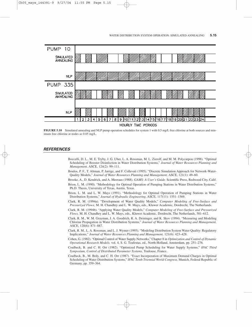
The actual pump operation schedules developed by the two optimization techniques are shown inFig. 5.10 for the case where both sources had 0.5 mg/L chlorine concentration.

As previously mentioned, the NLP solution where the sources had identical 0.5 mg/L concentra-tions resulted in a cost of $399.95 versus $429.53 which appears to be a preferred solution. However,a review of Fig. 5.10 reveals a problem with the NLP optimization. NLP is optimizing the amountof pumping time for a given period. This can result in several periods where the pumps operate onlypart of the time. This occurs during periods 2,3,8,10,12, and 14. In order to operate pumps more con-tinuously there would need to be some adjustment of the pumping schedule shown in Fig. 5.10,which could affect the ultimate cost of pumping.

5.6 SUMMARY AND CONCLUSIONS

Simulated annealing has been successfully linked with EPANET to optimize the operation of a waterdistribution system for hydraulic behavior and water quality.

5.14 CHAPTER FIVE

Ch05_mays_144381-9 9/27/04 11:55 PM Page 5.14

REFERENCES

Boccelli, D. L., M. E. Tryby, J. G. Uber, L. A. Rossman, M. L. Zierolf, and M. M. Polycarpou (1998). “OptimalScheduling of Booster Disinfection in Water Distribution Systems,” Journal of Water Resources Planning andManagement, ASCE, 124(2): 99–111.

Boulos, P. F., T. Altman, P. Jarrige, and F. Collevati (1995). “Discrete Simulation Approach for Network-Water-Quality Models,” Journal of Water Resources Planning and Management, ASCE, 121(1): 49–60.

Brooke, A., D. Kendrick, and A. Meeraus (1988). GAMS: A User’s Guide. Scientific Press, Redwood City, Calif.

Brion, L. M. (1990). “Methodology for Optimal Operation of Pumping Stations in Water Distribution Systems,”Ph.D. Thesis, University of Texas, Austin, Texas.

Brion, L. M. and L. W. Mays (1991). “Methodology for Optimal Operation of Pumping Stations in WaterDistribution Systems,” Journal of Hydraulic Engineering, ASCE, 117(11): 1551–1569.

Clark, R. M. (1994a). “Development of Water Quality Models,” Computer Modeling of Free-Surface andPressurized Flows, M. H. Chandhry and L. W. Mays, eds., Kluwer Academic, Dordrecht, The Netherlands.

Clark, R. M. (1994b). “Applying Water Quality Models,” Computer Modeling of Free-Surface and PressurizedFlows, M. H. Chandhry and L. W. Mays, eds., Kluwer Academic, Dordrecht, The Netherlands, 581–612.

Clark, R. M., W. M. Grayman, J. A. Goodrich, R. A. Deininger, and K. Skov (1994). “Measuring and ModelingChlorine Propagation in Water Distribution Systems,” Journal of Water Resources Planning and Management,ASCE, 120(6): 871–887.

Clark, R. M., L. A. Rossman, and L. J. Wymer (1995). “Modeling Distribution System Water Quality: RegulatoryImplications,” Journal of Water Resources Planning and Management, 121(6): 423–428.

Cohen, G. (1982). “Optimal Control of Water Supply Networks,” Chapter 8 in Optimization and Control of DynamicOperational Research Models, vol. 4, S. G. Tzafestas, ed., North-Holland, Amsterdam, pp. 251–276.

Coulbeck, B. and C. H. Orr (1982). “Optimized Pump Scheduling for Water Supply Systems,” IFAC ThirdSymposium, Control of Distributed Parameter Systems, Toulouse, France.

Coulbeck, B., M. Brdy, and C. H. Orr (1987). “Exact Incorporation of Maximum Demand Charges in OptimalScheduling of Water Distribution Systems,” IFAC Tenth Triennial World Congress, Munich, Federal Republic ofGermany, pp. 359–364.

WATER DISTRIBUTION SYSTEM OPERATION: SIMULATED ANNEALING 5.15

FIGURE 5.10 Simulated annealing and NLP pump operation schedules for system 1 with 0.5 mg/L free chlorine at both sources and min-imum free chlorine at nodes as 0.05 mg/L.

Ch05_mays_144381-9 9/27/04 11:55 PM Page 5.15

Dougherty, D. E. and R. A. Marryott (1991). “Optimal Groundwater Management—1. Simulated Annealing,”Water Resources Research, 27(10): 2493–2508.

Elton, A., L. F. Brammer, and N. S. Tansley (1995). “Water Quality Modeling in Distribution Networks,” JournalAWWA, 87(7): 44–52.

Goldman, F. E. (1998). “The Application of Simulated Annealing for Optimal Operation of Water DistributionSystems,” dissertation presented to Arizona State University, at Tempe, Arizona, in partial fulfillment of therequirements for the degree of Doctor of Philosophy.

Grayman, W., R. A. Dieninger, A. Green, P. Boulos, R. W. Bowcock, and C. Godwin (1996). “Water Quality andMixing Models for Tanks and Reservoirs,” Journal AWWA, 88(7): 60–73.

Huang, M.D., F. Romeo, and A. Sangiovanni-Vincentelli (1986). “An Efficient General Cooling Schedule forSimulated Annealing,” IEEE Transactions on Computer Aided Design, CAD-5(1): 381–384.

IAPMO (1994). Uniform Plumbing Code, International Association of Plumbing and Mechanical Officials.

Kirkpatrick, S. (1984). “Optimization by Simulated Annealing: Quantitative Studies,” Journal of Statistical Physics,34(5/6): 975–986.

Kirkpatrick, S., C. D. Gelatt, and M. P. Vecchi (1983). “Optimization by Simulated Annealing,” Science, 220(4598):671–680.

Lasdon, L. S., A. D. Waren, A. Jain, and M. Ratner (1978). “Design and Testing of a Generalized Reduced GradientCode for Nonlinear Programming,” ACM Transactions on Mathematical Software, 4(1): 34–50.

Li, Guihua and L. W. Mays (1995). “Differential Dynamic Programming for Estuariane Management,” Journalof Water Resources Planning and Management, ASCE, (121)6: 455–462.

Malcolm Pirnie (1996). Peoria Water Master Plan—Technical Memorandum No. 3—Distribution and FlowModel (Draft).

Nitivattananon, V., E. C. Sandowski, and R. G. Quimpo (1996). “Optimization of Water Supply System Operation.”Journal of Water Resources Planning and Management, ASCE, 122(5): 374–384.

Mays, L. W. and Y. K. Tung (1992). Hydrosystems Engineering and Management. McGraw-Hill, New York, pp.140–157.

Miller, L. H. and A. E. Quilici (1997). The Joy of C. John Wiley, New York.

Metropolis, N., A. Rosenbluth, M. Rosenbluth, A. Teller, and E. Teller (1953). “Equation of State Calculationsby Fast Computing Machines,” Journal of Chemical Physics, 21: 1087–1092.

Mulligan, A. E. and L. C. Brown (1998). “Genetic Algorithms for Calibrating Water Quality Models,” Journal ofEnvironmental Engineering, 124(3): 202–211.

Murtagh, B. A. and M. A. Saunders (1982). “A Projected Lagrangian Algorithm and Its Implementation for SparseNonlinear Constraints.” Mathematical Programming Study, 16: 84–117.

Murtagh, B. A. and M. A. Saunders (1987). Minus 5.1 User’s Guide. Stanford Optimization Lab., StanfordUniversity, Stanford, Calif.

Okun, D. A. (1996). “From Cholera to Cancer to Cryptosporidiosis,” Journal of Environmental Engineering,122(6): 453–458.

Ormsbee, L. E., editor (1991). “Energy Efficient Operation of Water Distribution Systems,” A Report by the ASCETask Committee on the Optimal Operation of Water Distribution Systems, Univ. of Kentucky, Lexington, Ky.

Ormsbee, L. E. and K. E. Lansey (1994). “Optimal Control of Water Supply Pumping Systems,” Journal of WaterResources Planning and Management, 120(2): 237–252.

Ormsbee, L. E. and S. L. Reddy (1995). “Nonlinear Heuristic for Pump Operations,” Journal of Water ResourcesPlanning and Management, 121(4): 302–309.

Ormsbee, L. E., T. M. Walski, D. V. Chase, and W. W. Sharp (1989). “Methodology for Improving PumpOperation Efficiency,” Journal of Water Resources Planning and Management, 115(2): 148–164.

Ostfeld, A. and U. Shamir (1993). “Optimal Operation of Multiquality Networks. I: Steady State-Conditions,”Journal of Water Resources Planning and Management, 119(6): 645–662.

Ostfeld, A. and U. Shamir (1993). “Optimal Operation of Multiquality Networks. II: Unsteady Conditions,”Journal of Water Resources Planning and Management, 119(6): 663–684.

Otten, R. H. J. M. and L. P. P. P. van Ginnekin (1989). The Annealing Algorithm, Kluwer Academic, Boston.

Pontius, F. W. (1996). “Overview of the Safe Drinking Water Act Amendments of 1996,” Journal AWWA, 88(10):22–33.

5.16 CHAPTER FIVE

Ch05_mays_144381-9 9/27/04 11:55 PM Page 5.16

Rossman, L. A. (1993). EPANET Users Manual, Risk Reduction Engineering Laboratory, Office of Research andDevelopment, U.S. Environmental Protection Agency, Cincinnati, Ohio.

Rossman, L. A. and P. F. Boulos (1996). “Numerical Methods for Modeling Water Quality in Distribution Systems:A Comparison,” Journal of Water Resources Planning and Management, 122(2): 137–146.

Rossman, L. A., P. F. Boulos, and T. Altman (1993). “The Discrete Volume Element Method for Network WaterQuality Models,” Journal of Water Resources Planning and Management, 119(5): 505–517.

Rossman, L. A., R. W. Clark, and W. M. Grayman. (1994). “Modeling Chlorine Residuals in Drinking-WaterDistribution Systems,” Journal of Environmental Engineering, 120(4): 803–820.

Sadowski, E., V. Nitivattananon, and R. E. Quimpo (1995). “Computer-Generated Optimal Pumping Schedule,”Journal AWWA, 87(7): 53–63.

Sakarya, A. B. (1998). “Optimal Operation of Water Distribution Systems for Water Quality Purposes,” disser-tation presented to Arizona State University, at Tempe, Arizona, in partial fulfillment of the requirements for thedegree of Doctor of Philosophy.

Sakarya, A. B. and L. W. Mays (2000). “Optimal Operation of Water Distribution Pumps Considering WaterQuality,” Journal of Water Resources Planning and Management, 126(4): 210–220.

van Laarhoven, P. J. M. (1980). Theoretical and Computational Aspects of Simulated Annealing, Center forMathematics and Computer Science, Amsterdam, The Netherlands.

Vasconcelos, J. J., P. F. Boulos, W. M. Grayman, L. Kiene, O. Wable, P. Biswas, A. Bhari, L. A. Rossman, R. M.Clark, and J. A. Goodrich (1996). Characterization and Modeling of Chlorine Decay in Distribution Systems,AWWA Research Foundation and American Water Works Association, Denver, Colo. pp. 258–271.

Vidal, René V. V., ed. (1993). Applied Simulated Annealing, Springer-Verlag, New York.

Wanakule, N., L. W. Mays, and L. S. Lasdon (1986). “Optimal Management of Large-Scale Aquifers: Methodologyand Applications.” Water Resources Research, 22(4): 447–465.

Wiffen, G. J. and C. A. Shoemaker (1993). “Nonlinear Weighted Feedback Control of Groundwater Remediationunder Uncertainty,” Water Resources Research, 29(9): 3277–3289.

Wood, D. J. (1980). User’s Manual—Computer Analysis of Flow in Pipe Networks Including Extended PeriodSimulations, University of Kentucky.

Zessler, U. and U. Shamir (1989). “Optimal Operation of Water Distribution Systems,” Journal of Water ResourcesPlanning and Management, 115(6): 735–752.

WATER DISTRIBUTION SYSTEM OPERATION: SIMULATED ANNEALING 5.17

Ch05_mays_144381-9 9/27/04 11:55 PM Page 5.17

Ch05_mays_144381-9 9/27/04 11:55 PM Page 5.18