Embed Size (px)
Citation preview
WWaatteerr QQuuaalliittyy AAnnaallyyssiiss SSiimmuullaattiioonn PPrrooggrraamm ((WWAASSPP))
Version 6.0 DDRRAAFFTT:: UUsseerr’’ss MMaannuuaall
By
Tim A. Wool
Robert B. Ambrose1
James L. Martin2
Edward A. Comer3
US Environmental Protection Agency – Region 4 Atlanta, GA
1Environmental Research Laboratory
Athens, GA
2USACE – Waterways Experiment Station Vicksburg, MS
3Tetra Tech, Inc.
Atlanta, GA
DRAFT: Water Quality Analysis Simulation Program (WASP) Version 6.0
i
Table of Contents
1. Forward _________________________________________________________1-1
2. Acknowledgements_________________________________________________2-2
3. Introduction ______________________________________________________3-3
3.1. Overview of the WASP6 Modeling System ___________________________ 3-3
3.2. Installation____________________________________________________ 3-5
3.3. Technical Support ______________________________________________ 3-5
3.4. Tool Bar Definition _____________________________________________ 3-5
3.5. File Menu_____________________________________________________ 3-7 3.5.1. Importing Old WASP Input Files __________________________________________ 3-7 3.5.2. Exporting Old WASP Input Files __________________________________________ 3-8 3.5.3. User Preferences ______________________________________________________ 3-8
3.6. Project Files___________________________________________________ 3-9 3.6.1. New ________________________________________________________________ 3-9 3.6.2. Open ______________________________________________________________ 3-10 3.6.3. Edit _______________________________________________________________ 3-10 3.6.4. Save_______________________________________________________________ 3-10 3.6.5. Save-as_____________________________________________________________ 3-10
3.7. Input Parameterization _________________________________________ 3-11 3.7.1. Data Set Description___________________________________________________ 3-12 3.7.2. Model Type _________________________________________________________ 3-12 3.7.3. Comments __________________________________________________________ 3-12 3.7.4. Restart Options_______________________________________________________ 3-13 3.7.5. Date and Times ______________________________________________________ 3-13 3.7.6. Non-Point Source File _________________________________________________ 3-13 3.7.7. Hydrodynamics ______________________________________________________ 3-13
3.8. Systems _____________________________________________________ 3-14 3.8.1. System Options ______________________________________________________ 3-15 3.8.2. Dispersion/Flow Bypass________________________________________________ 3-16 3.8.3. Density_____________________________________________________________ 3-16 3.8.4. Maximum Concentration _______________________________________________ 3-16 3.8.5. Boundary/Load Scale & Conversion Factor _________________________________ 3-16
3.9. Segmentation Screen___________________________________________ 3-17 3.9.1. Segment Definition ___________________________________________________ 3-17 3.9.2. Segment Environmental Parameters _______________________________________ 3-19 3.9.3. Initial Concentrations__________________________________________________ 3-20 3.9.4. Fraction Dissolved ____________________________________________________ 3-21
3.10. Segment Parameter Scale Factors _________________________________ 3-22
3.11. Dispersion ___________________________________________________ 3-23 3.11.1. Exchange Fields ___________________________________________________ 3-24 3.11.2. Dispersion Function_________________________________________________ 3-24 3.11.3. Dispersion Time Function ____________________________________________ 3-25
3.12. Flows _______________________________________________________ 3-25 3.12.1. Flow Function _____________________________________________________ 3-27 3.12.2. Flow Time Function ________________________________________________ 3-27
DRAFT: Water Quality Analysis Simulation Program (WASP) Version 6.0
ii
3.13. Boundaries___________________________________________________ 3-27 3.13.1. Boundary Time Function _____________________________________________ 3-28
3.14. Loads _______________________________________________________ 3-28 3.14.1. Load Time Function ________________________________________________ 3-29
3.15. Loads Scale and Conversion _____________________________________ 3-29 3.15.1. Time Step ________________________________________________________ 3-30
3.16. Print Interval_________________________________________________ 3-31
3.17. Time Functions _______________________________________________ 3-32
3.18. Constants____________________________________________________ 3-33
3.19. Fill/Calculate & Graphing _______________________________________ 3-35 3.19.1. Toolbar Definition __________________________________________________ 3-38
3.20. Validity Check________________________________________________ 3-38
3.21. Model Execution ______________________________________________ 3-39
4. Visual Graphic Post -Processor ______________________________________4-42
4.1. Main Toolbar_________________________________________________ 4-42
4.2. Model Output Selection_________________________________________ 4-43 4.2.1. Opening Model Output_________________________________________________ 4-43
4.3. Spatial Graphical Analysis_______________________________________ 4-45 4.3.1. Overview___________________________________________________________ 4-45 4.3.2. Spatial Grid Toolbar___________________________________________________ 4-46 4.3.3. Geographical Information System Interface _________________________________ 4-47 4.3.4. BMG File Creation with Digitize _________________________________________ 4-48 4.3.5. Controlling Spatial Analysis _____________________________________________ 4-49 4.3.6. Selecting Dataset _____________________________________________________ 4-51 4.3.7. Selecting Slice/Geometry _______________________________________________ 4-52 4.3.8. Selecting Variable ____________________________________________________ 4-52 4.3.9. Selecting Time _______________________________________________________ 4-53 4.3.10. Palette ___________________________________________________________ 4-53 4.3.11. Animation ________________________________________________________ 4-53 4.3.12. Plot Mode ________________________________________________________ 4-53 4.3.13. GIS Configuration __________________________________________________ 4-54 4.3.14. Layers ___________________________________________________________ 4-54 4.3.15. GIS Toolbar_______________________________________________________ 4-55
4.4. x/y Plot______________________________________________________ 4-56 4.4.1. Overview___________________________________________________________ 4-56 4.4.2. Toolbar ____________________________________________________________ 4-56 4.4.3. Creating x/y Plot _____________________________________________________ 4-57 4.4.4. OK/Cancel __________________________________________________________ 4-67 4.4.5. Zooming the Axes ____________________________________________________ 4-68 4.4.6. Adding an Additional Curve_____________________________________________ 4-71 4.4.7. Color/Black & White View _____________________________________________ 4-72 4.4.8. Observed/Measured Data _______________________________________________ 4-72 4.4.9. Printing Results ______________________________________________________ 4-75 4.4.10. Creating Tabled Data ________________________________________________ 4-76 4.4.11. Curve Calculations _________________________________________________ 4-77
5. The Basic Water Quality Model ______________________________________5-1
DRAFT: Water Quality Analysis Simulation Program (WASP) Version 6.0
iii
5.1. General Mass Balance Equation ___________________________________ 5-1
5.2. The Model Network _____________________________________________ 5-3
5.3. The Model Transport Scheme _____________________________________ 5-7
5.4. Application of the Model_________________________________________ 5-8
6. Chemical Tracer Transport __________________________________________6-1
6.1. Overview of WASP6 Tracer Transport ______________________________ 6-1
6.2. Transport Processes_____________________________________________ 6-1 6.2.1. Hydrodynamic Linkage _________________________________________________ 6-2 6.2.2. Hydraulic Geometry ____________________________________________________ 6-4 6.2.3. Pore Water Advection __________________________________________________ 6-7 6.2.4. Water Column Dispersion _______________________________________________ 6-7 6.2.5. Pore Water Diffusion ___________________________________________________ 6-8 6.2.6. Boundary Processes ____________________________________________________ 6-9 6.2.7. Loading Processes ____________________________________________________ 6-10 6.2.8. Nonpoint Source Linkage _______________________________________________ 6-11 6.2.9. Initial Conditions _____________________________________________________ 6-12
6.3. Model Implementation__________________________________________ 6-13
6.4. Model Input Parameters ________________________________________ 6-13 6.4.1. Environment Parameters _______________________________________________ 6-13 6.4.2. Transport Parameters __________________________________________________ 6-17 6.4.3. Boundary Parameters __________________________________________________ 6-18 6.4.4. Transformation Parameters ______________________________________________ 6-19 6.4.5. External Input Files ___________________________________________________ 6-19
7. Sediment Transport ________________________________________________7-1
7.1. Overview of WASP Sediment Transport _____________________________ 7-1 7.1.1. Sediment Transport Processes ____________________________________________ 7-1 7.1.2. Sediment Loading _____________________________________________________ 7-4 7.1.3. The Sediment Bed _____________________________________________________ 7-5
7.2. Model Implementation___________________________________________ 7-9 7.2.1. Model Input Parameters _________________________________________________ 7-9 7.2.2. Environment Parameters_________________________________________________ 7-9 7.2.3. Boundary Parameters __________________________________________________ 7-10 7.2.4. Transformation Parameters ______________________________________________ 7-11
8. Dissolved Oxygen__________________________________________________8-1
8.1. Overview of WASP6 Dissolved Oxygen______________________________ 8-1
8.2. Dissolved Oxygen Processes_______________________________________ 8-3 8.2.1. Reaeration ___________________________________________________________ 8-4 8.2.2. Carbonaceous Oxidation_________________________________________________ 8-7 8.2.3. Nitrification __________________________________________________________ 8-9 8.2.4. Denitrification _______________________________________________________ 8-10 8.2.5. Settling ____________________________________________________________ 8-10 8.2.6. Phytoplankton Growth _________________________________________________ 8-10 8.2.7. Phytoplankton Death __________________________________________________ 8-11 8.2.8. Sediment Oxygen Demand ______________________________________________ 8-11
8.3. Model Implementation__________________________________________ 8-14 8.3.1. Streeter-Phelps_______________________________________________________ 8-14

DRAFT: Water Quality Analysis Simulation Program (WASP) Version 6.0
iv
8.3.2. Environment Parameters________________________________________________ 8-15 8.3.3. Transport Parame ters __________________________________________________ 8-15 8.3.4. Boundary Parameters __________________________________________________ 8-16 8.3.5. Transformation Parameters ______________________________________________ 8-16
8.4. Modified Streeter-Phelps ________________________________________ 8-18 8.4.1. Environment Parameters________________________________________________ 8-20 8.4.2. Transport Parameters __________________________________________________ 8-20 8.4.3. Boundary Parameters __________________________________________________ 8-21 8.4.4. Transformation Parameters ______________________________________________ 8-22
8.5. Full Linear DO Balance_________________________________________ 8-22 8.5.1. Environment Parameters________________________________________________ 8-24 8.5.2. Transport Parameters __________________________________________________ 8-24 8.5.3. Boundary Parameters __________________________________________________ 8-25 8.5.4. Transformation Parameters ______________________________________________ 8-26
8.6. Nonlinear DO Balance __________________________________________ 8-26
9. Eutrophication ____________________________________________________9-1
9.1. Overview of WASP6 Eutrophication ________________________________ 9-1 9.1.1. Phosphorus Cycle ______________________________________________________ 9-3 9.1.2. Nitrogen Cycle ________________________________________________________ 9-3 9.1.3. Dissolved Oxygen _____________________________________________________ 9-3 9.1.4. Phytoplankton Kinetics _________________________________________________ 9-3 9.1.5. Phytoplankton Growth __________________________________________________ 9-5 9.1.6. Phytoplankton Death __________________________________________________ 9-12 9.1.7. Phytoplankton Settling _________________________________________________ 9-14 9.1.8. Summary ___________________________________________________________ 9-14 9.1.9. Stoichiometry and Uptake Kinetics________________________________________ 9-15
9.2. The Phosphorus Cycle __________________________________________ 9-16 9.2.1. Phytoplankton Growth _________________________________________________ 9-18 9.2.2. Phytoplankton Death __________________________________________________ 9-18 9.2.3. Mineralization _______________________________________________________ 9-18 9.2.4. Sorption ____________________________________________________________ 9-18 9.2.5. Settling ____________________________________________________________ 9-21
9.3. The Nitrogen Cycle ____________________________________________ 9-21 9.3.1. Phytoplankton Growth _________________________________________________ 9-23 9.3.2. Phytoplankton Death __________________________________________________ 9-24 9.3.3. Mineralization _______________________________________________________ 9-25 9.3.4. Settling ____________________________________________________________ 9-25 9.3.5. Nitrification _________________________________________________________ 9-25 9.3.6. Denitrification _______________________________________________________ 9-26
9.4. The Dissolved Oxygen Balance ___________________________________ 9-26 9.4.1. Benthic - Water Column Interactions ______________________________________ 9-26 9.4.2. Benthic Simulation____________________________________________________ 9-28
9.5. Model Implementation__________________________________________ 9-32
9.6. Simple Eutrophication Kinetics ___________________________________ 9-33 9.6.1. Environment Parameters________________________________________________ 9-34 9.6.2. Transport Parameters __________________________________________________ 9-34 9.6.3. Boundary Parameters __________________________________________________ 9-35 9.6.4. Transformation Parameters ______________________________________________ 9-36
9.7. Intermediate Eutrophication Kinetics ______________________________ 9-38
DRAFT: Water Quality Analysis Simulation Program (WASP) Version 6.0
v
9.7.1. Environment Parameters________________________________________________ 9-39 9.7.2. Transport Parameters __________________________________________________ 9-39 9.7.3. Boundary Parameters __________________________________________________ 9-39 9.7.4. Transformation Parameters ______________________________________________ 9-40
9.8. Intermediate Eutrophication Kinetics with Benthos ___________________ 9-43
10. Simple Toxicants _______________________________________________10-1
10.1. Simple Transformation Kinetics __________________________________ 10-3 10.1.1. Option 1: Total Lumped First Order Decay _______________________________ 10-3 10.1.2. Option 2: Individual First Order Transformation ___________________________ 10-4
10.2. Equilibrium Sorption___________________________________________ 10-4
10.3. Transformations and Daughter Products____________________________ 10-6
10.4. Model Implementation__________________________________________ 10-7 10.4.1. Model Input Parameters ______________________________________________ 10-7 10.4.2. Environment Parameters _____________________________________________ 10-7 10.4.3. Transport Parameters ________________________________________________ 10-8 10.4.4. Boundary Parameters ________________________________________________ 10-9 10.4.5. Transformation Parameters __________________________________________ 10-10
11. Organic Chemicals______________________________________________11-1
11.1. TOXI Reactions and Transformations ______________________________ 11-3
11.2. Model Implementation__________________________________________ 11-4 11.2.1. Model Input Parameters ______________________________________________ 11-4 11.2.2. Transformation Parameters ___________________________________________ 11-4
11.3. Ionization____________________________________________________ 11-6 11.3.1. Overview of TOXI Ionization Reactions _________________________________ 11-6
11.4. Implementation ______________________________________________ 11-10
11.5. Equilibrium Sorption__________________________________________ 11-11 11.5.1. Overview of TOXI Sorption Reactions__________________________________ 11-12 11.5.2. Computation of Partition Coefficients __________________________________ 11-15 11.5.3. Option 1. Measured Partition Coefficients. ______________________________ 11-15 11.5.4. Option 2. Input of Organic Carbon Partition Coefficient.____________________ 11-15 11.5.5. Option 4. Computation of Solids Dependant Partitioning. ___________________ 11-16 11.5.6. Option 1: Measured Partition Coefficients. ______________________________ 11-18 11.5.7. Option 2: Input of Organic Carbon Partition Coefficient.____________________ 11-18 11.5.8. Option 3: Computation of the Organic Carbon Partition Coefficient. ___________ 11-18 11.5.9. Option 4: Solids Dependant Partitioning. _______________________________ 11-19
11.6. Volatilization ________________________________________________ 11-19 11.6.1. Overview of TOXI Volatilization______________________________________ 11-20 11.6.2. Volatilization Option 1. _____________________________________________ 11-22 11.6.3. Volatilization Option 2. _____________________________________________ 11-22 11.6.4. Volatilization Option 3. _____________________________________________ 11-23 11.6.5. Volatilization Option 4. _____________________________________________ 11-23 11.6.6. Volatilization Option 5. _____________________________________________ 11-25 11.6.7. Volatilization Option 1 _____________________________________________ 11-28 11.6.8. Volatilization Option 2 _____________________________________________ 11-28 11.6.9. Volatilization Option 3 _____________________________________________ 11-29 11.6.10. Volatilization Option 4 _____________________________________________ 11-29 11.6.11. Volatilization Option 5 _____________________________________________ 11-30
DRAFT: Water Quality Analysis Simulation Program (WASP) Version 6.0
vi
11.7. Hydrolysis __________________________________________________ 11-30 11.7.1. Overview of TOXI Hydrolysis Reactions________________________________ 11-30 11.7.2. Option 1. First Order Hydrolysis. _____________________________________ 11-30 11.7.3. Option 2. Second Order Hydrolysis. ___________________________________ 11-30
11.8. Photolysis___________________________________________________ 11-34 11.8.1. Overview of TOXI Photolysis Reactions ________________________________ 11-34 11.8.2. Photolysis Option 1.________________________________________________ 11-35 11.8.3. Photolysis Option 2.________________________________________________ 11-38 11.8.4. Photolysis Option 1 ________________________________________________ 11-39 11.8.5. Photolysis Option 2 ________________________________________________ 11-41
11.9. Oxidation___________________________________________________ 11-43 11.9.1. Overview of TOXI Oxidation Reactions ________________________________ 11-43
11.10. Biodegradation ____________________________________________ 11-45 11.10.1. Overview of TOXI Biodegradation Reactions ____________________________ 11-46
11.11. Extra Reaction_____________________________________________ 11-49 11.11.1. Overview of TOXI Extra Reaction_____________________________________ 11-49
12. REFERENCES ________________________________________________12-1
DRAFT: Water Quality Analysis Simulation Program (WASP) Version 6.0
1-1
1. Forward
WASP6 is an enhanced Windows version of the USEPA Water Quality Analysis Simulation Program (WASP). WASP6 has been developed to aid modelers in the implementation of WASP. WASP6 has features including a pre-processor, a rapid data processor, and a graphical post-processor that enable the modeler to run WASP more quickly and easily and evaluate model results both numerically and graphically. With WASP6, model execution can be performed up to ten times faster than the previous USEPA DOS version of WASP. Nonetheless, WASP6 uses the same algorithms to solve water quality problems as those used in the DOS version of WASP.
WASP6 contains 1) a user-friendly Windows-based interface, 2) a pre-processor to assist modelers in the processing of data into a format that can be used in WASP, 3) high-speed WASP eutrophication and organic chemical model processors, and 4) a graphical post-processor for the viewing of WASP results and comparison to observed field data.
Because of the architecture utilized in the design of WASP6 it is going to be relatively easy to develop other kinetic modules for WASP. Currently, we are planning on the development of an enhanced eutrophication model that will include the addition of the following state variables: 2 additional algal groups, salinity, full heat balance, coliforms, second BOD group, sediment digenesis model.
DRAFT: Water Quality Analysis Simulation Program (WASP) Version 6.0
2-2
2. Acknowledgements
The US EPA would like to acknowledge the generous donation that ASci Corporation has made by releasing the Windows of WASP to EPA and the public domain. Their realization of the environmental good that will come from the use of this model and their unselfish attitude should be commended.
Furthermore, the authors would like to recognize Mr. Jim Greenfield, EPA Region 4 for his support and encouragement in the development and enhancement of WASP6. The authors would like to express gratitude to Mr. Mohammed Lahlomo for his support and efforts in bringing WASP6 to the public domain.
DRAFT: Water Quality Analysis Simulation Program (WASP) Version 6.0
3-3
3. Introduction
The Water Quality Analysis Simulation Program— (WASP6), an enhancement of the original WASP (Di Toro et al., 1983; Connolly and Winfield, 1984; Ambrose, R.B. et al., 1988). This model helps users interpret and predict water quality responses to natural phenomena and man-made pollution for various pollution management decisions. WASP6 is a dynamic compartment-modeling program for aquatic systems, including both the water column and the underlying benthos. The time-varying processes of advection, dispersion, point and diffuse mass loading, and boundary exchange are represented in the basic program.
Water quality processes are represented in special kinetic subroutines that are either chosen from a library or written by the user. WASP is structured to permit easy substitution of kinetic subroutines into the overall package to form problem-specific models. WASP6 comes with two such models -- TOXI for toxicants and EUTRO for conventional water quality. Earlier versions of WASP have been used to examine eutrophication of Tampa Bay; phosphorus loading to Lake Okeechobee; eutrophication of the Neuse River and estuary; eutrophication and PCB pollution of the Great Lakes (Thomann, 1975; Thomann et al., 1976; Thomann et al, 1979; Di Toro and Connolly, 1980), eutrophication of the Potomac Estuary (Thomann and Fitzpatrick, 1982), kepone pollution of the James River Estuary (O'Connor et al., 1983), volatile organic pollution of the Delaware Estuary (Ambrose, 1987), and heavy metal pollution of the Deep River, North Carolina (JRB, 1984). In addition to these, numerous applications are listed in Di Toro et al., 1983.
The flexibility afforded by the Water Quality Analysis Simulation Program is unique. WASP6 permits the modeler to structure one, two, and three dimensional models; allows the specification of time-variable exchange coefficients, advective flows, waste loads and water quality boundary conditions; and permits tailored structuring of the kinetic processes, all within the larger modeling framework without having to write or rewrite large sections of computer code. The two operational WASP6 models, TOXI and EUTRO, are reasonably general. In addition, users may develop new kinetic or reactive structures. This however requires an additional measure of judgment, insight, and programming experience on the part of the modeler. The kinetic subroutine in WASP (denoted "WASPB"), is kept as a separate section of code, with its own subroutines if desired.
3.1. Overview of the WASP6 Modeling System
The WASP6 system consists of two stand-alone computer programs, DYNHYD5 and WASP6, which can be run in conjunction or separately. The hydrodynamics program, DYNHYD5, simulates the movement of water while the water quality program, WASP6, simulates the movement and interaction of pollutants within the water. While DYNHYD5 is delivered with WASP6, other hydrodynamic programs have also been linked with WASP. RIVMOD handles unsteady flow in one-dimensional rivers, while
DRAFT: Water Quality Analysis Simulation Program (WASP) Version 6.0
3-4
SED3D handles unsteady, three-dimensional flow in lakes and estuaries (contact CEAM for availability).
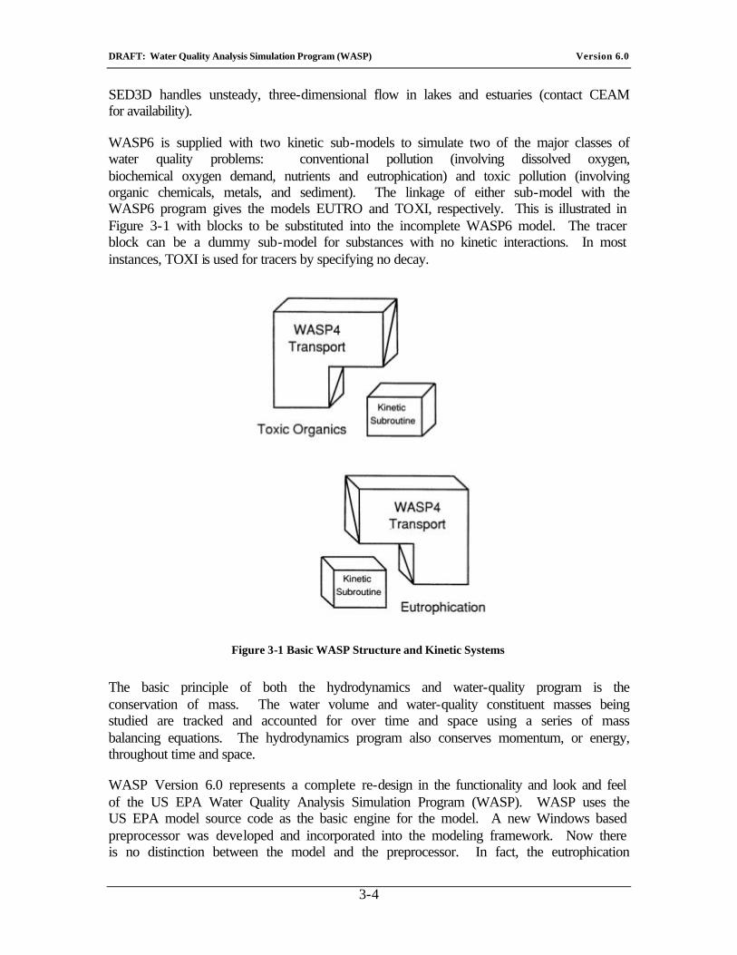
WASP6 is supplied with two kinetic sub-models to simulate two of the major classes of water quality problems: conventional pollution (involving dissolved oxygen, biochemical oxygen demand, nutrients and eutrophication) and toxic pollution (involving organic chemicals, metals, and sediment). The linkage of either sub-model with the WASP6 program gives the models EUTRO and TOXI, respectively. This is illustrated in Figure 3-1 with blocks to be substituted into the incomplete WASP6 model. The tracer block can be a dummy sub-model for substances with no kinetic interactions. In most instances, TOXI is used for tracers by specifying no decay.
Figure 3-1 Basic WASP Structure and Kinetic Systems
The basic principle of both the hydrodynamics and water-quality program is the conservation of mass. The water volume and water-quality constituent masses being studied are tracked and accounted for over time and space using a series of mass balancing equations. The hydrodynamics program also conserves momentum, or energy, throughout time and space.
WASP Version 6.0 represents a complete re-design in the functionality and look and feel of the US EPA Water Quality Analysis Simulation Program (WASP). WASP uses the US EPA model source code as the basic engine for the model. A new Windows based preprocessor was developed and incorporated into the modeling framework. Now there is no distinction between the model and the preprocessor. In fact, the eutrophication
DRAFT: Water Quality Analysis Simulation Program (WASP) Version 6.0
3-5
model is a dynamic link library (DLL) that is executed by the preprocessor. WASP no longer requires input files, the data needed to execute the model is passed to the model DLL using dynamic data exchange. The model input dataset reading routines have been removed from the model. This was done to make a more efficient means of storing the model-input dataset and not worrying about all of the formatting issues associated with the DOS based model.
3.2. Installation
The WASP6 installation is accomplished much like any other Windows software installation. To initiate the installation:
1. Place the WASP6 CD in your CD-ROM drive.
2. Select Start/Run from the Windows menu.
3. Enter d:/setup (If your CD-ROM drive is not drive D, type the appropriate letter instead).
4. Choose OK.
5. Follow the instructions on the screen prompts to complete the installation.
3.3. Technical Support
3.4. Tool Bar Definition
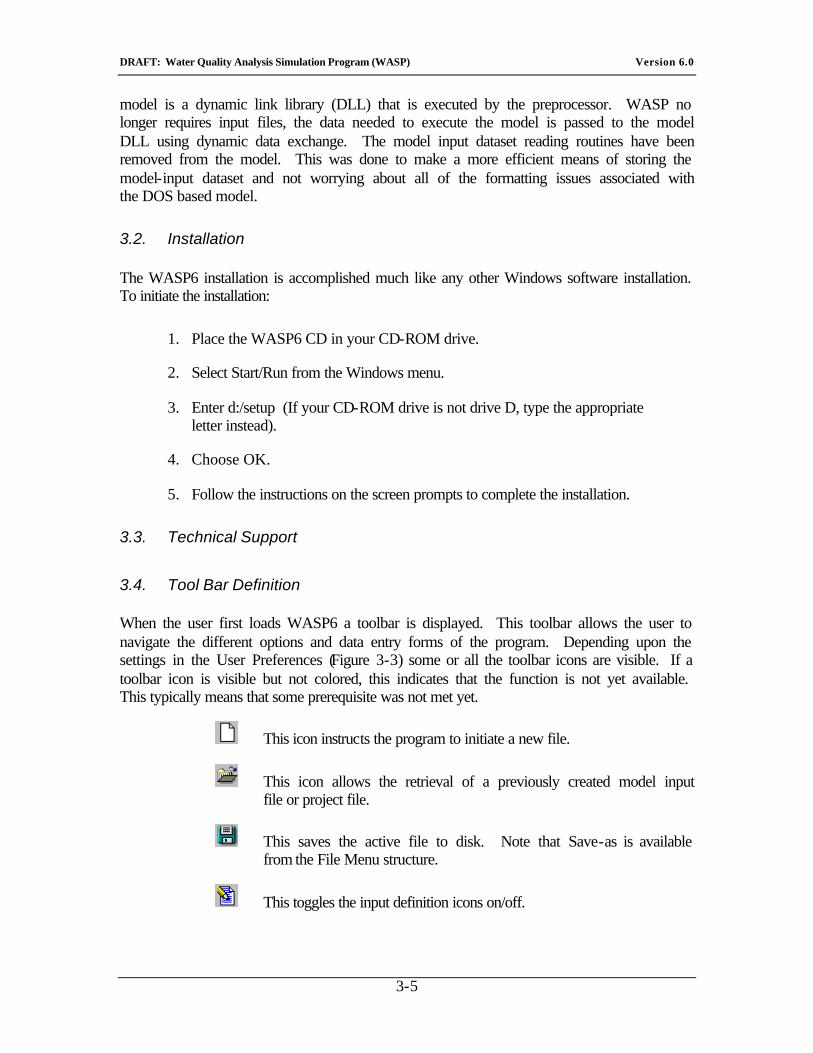
When the user first loads WASP6 a toolbar is displayed. This toolbar allows the user to navigate the different options and data entry forms of the program. Depending upon the settings in the User Preferences (Figure 3-3) some or all the toolbar icons are visible. If a toolbar icon is visible but not colored, this indicates that the function is not yet available. This typically means that some prerequisite was not met yet.
This icon instructs the program to initiate a new file.
This icon allows the retrieval of a previously created model input file or project file.
This saves the active file to disk. Note that Save-as is available from the File Menu structure.
This toggles the input definition icons on/off.
DRAFT: Water Quality Analysis Simulation Program (WASP) Version 6.0
3-6
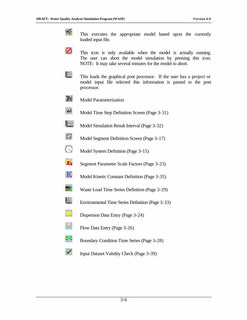
This executes the appropriate model based upon the currently loaded input file.
This icon is only available when the model is actually running. The user can abort the model simulation by pressing this icon. NOTE: It may take several minutes for the model to abort.
This loads the graphical post processor. If the user has a project or model input file selected this information is passed to the post processor.
Model Parameterization
Model Time Step Definition Screen (Page 3-31)
Model Simulation Result Interval (Page 3-32)
Model Segment Definition Screen (Page 3-17)
Model System Definition (Page 3-15)
Segment Parameter Scale Factors (Page 3-23)
Model Kinetic Constant Definition (Page 3-35)
Waste Load Time Series Definition (Page 3-29)
Environmental Time Series Definition (Page 3-33)
Dispersion Data Entry (Page 3-24)
Flow Data Entry (Page 3-26)
Boundary Condition Time Series (Page 3-28)
Input Dataset Validity Check (Page 3-39)
DRAFT: Water Quality Analysis Simulation Program (WASP) Version 6.0
3-7
3.5. File Menu
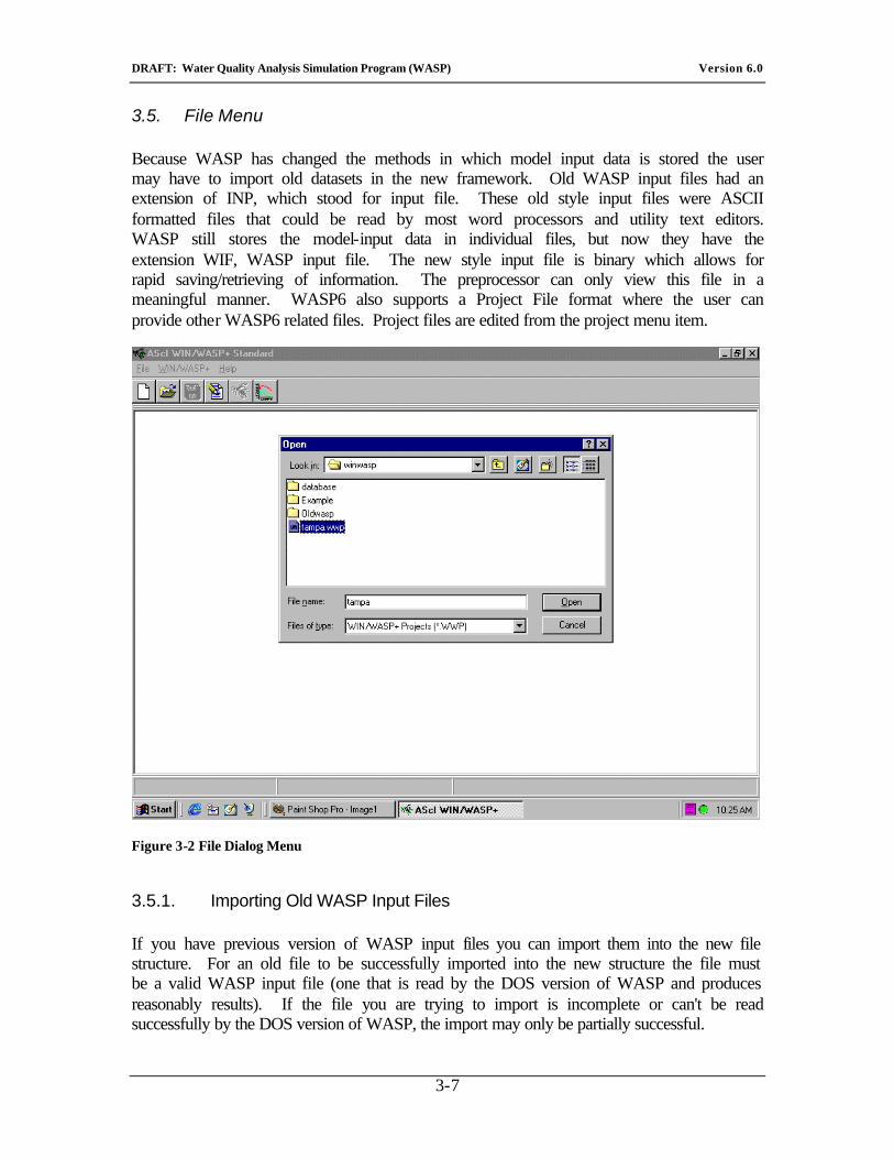
Because WASP has changed the methods in which model input data is stored the user may have to import old datasets in the new framework. Old WASP input files had an extension of INP, which stood for input file. These old style input files were ASCII formatted files that could be read by most word processors and utility text editors. WASP still stores the model-input data in individual files, but now they have the extension WIF, WASP input file. The new style input file is binary which allows for rapid saving/retrieving of information. The preprocessor can only view this file in a meaningful manner. WASP6 also supports a Project File format where the user can provide other WASP6 related files. Project files are edited from the project menu item.
Figure 3-2 File Dialog Menu
3.5.1. Importing Old WASP Input Files
If you have previous version of WASP input files you can import them into the new file structure. For an old file to be successfully imported into the new structure the file must be a valid WASP input file (one that is read by the DOS version of WASP and produces reasonably results). If the file you are trying to import is incomplete or can't be read successfully by the DOS version of WASP, the import may only be partially successful.
DRAFT: Water Quality Analysis Simulation Program (WASP) Version 6.0
3-8
To import a file the user should open the old file with the preprocessor. This will initiate the import of the data. The user will see a description of activities as the import progresses.
3.5.2. Exporting Old WASP Input Files
WASP6 can export a WIF file format to the previous WASP file format. This would be useful for sharing input files with other people who do not use WASP6. The Export function is available from the file menu; you will be required to provide a filename in which to export the information.
3.5.3. User Preferences
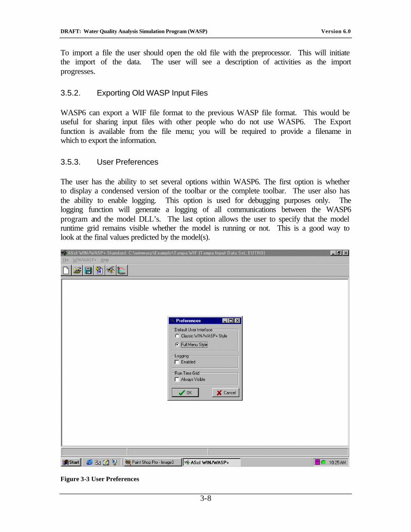
The user has the ability to set several options within WASP6. The first option is whether to display a condensed version of the toolbar or the complete toolbar. The user also has the ability to enable logging. This option is used for debugging purposes only. The logging function will generate a logging of all communications between the WASP6 program and the model DLL’s. The last option allows the user to specify that the model runtime grid remains visible whether the model is running or not. This is a good way to look at the final values predicted by the model(s).
Figure 3-3 User Preferences
DRAFT: Water Quality Analysis Simulation Program (WASP) Version 6.0
3-9
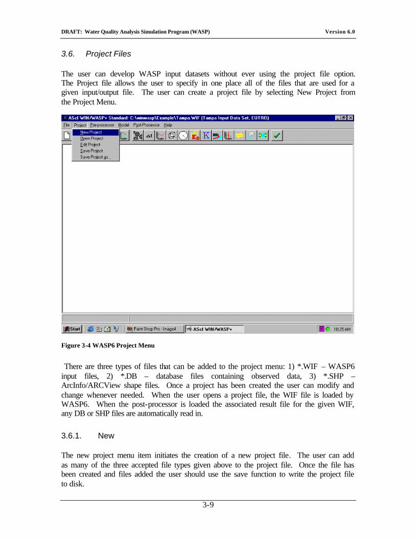
3.6. Project Files
The user can develop WASP input datasets without ever using the project file option. The Project file allows the user to specify in one place all of the files that are used for a given input/output file. The user can create a project file by selecting New Project from the Project Menu.
Figure 3-4 WASP6 Project Menu
There are three types of files that can be added to the project menu: 1) *.WIF – WASP6 input files, 2) *.DB – database files containing observed data, 3) *.SHP – ArcInfo/ARCView shape files. Once a project has been created the user can modify and change whenever needed. When the user opens a project file, the WIF file is loaded by WASP6. When the post-processor is loaded the associated result file for the given WIF, any DB or SHP files are automatically read in.
3.6.1. New
The new project menu item initiates the creation of a new project file. The user can add as many of the three accepted file types given above to the project file. Once the file has been created and files added the user should use the save function to write the project file to disk.
DRAFT: Water Quality Analysis Simulation Program (WASP) Version 6.0
3-10
3.6.2. Open
This menu item allows the user to open a previously created project file. Once open is selected the user is given a standard Windows file dialog box. Note that project files have the extension of *.WWP.
3.6.3. Edit
The edit menu item allows the user to modify the contents of the opened project file. The users can remove/add files to the project.
3.6.4. Save
The save function writes the project file information to disk. When this option is selected the file is written without user intervention.
3.6.5. Save-as
The Save-as function allows the user to save the previously loaded project file to another filename. This is useful when conducting sensitivity analysis and do not want to lose the initial project. When the user selects the Save-as function they are presented with a standard Windows file dialog box.
DRAFT: Water Quality Analysis Simulation Program (WASP) Version 6.0
3-11
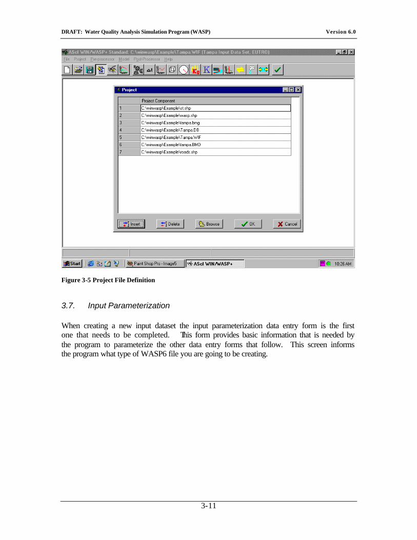
Figure 3-5 Project File Definition
3.7. Input Parameterization
When creating a new input dataset the input parameterization data entry form is the first one that needs to be completed. This form provides basic information that is needed by the program to parameterize the other data entry forms that follow. This screen informs the program what type of WASP6 file you are going to be creating.
DRAFT: Water Quality Analysis Simulation Program (WASP) Version 6.0
3-12
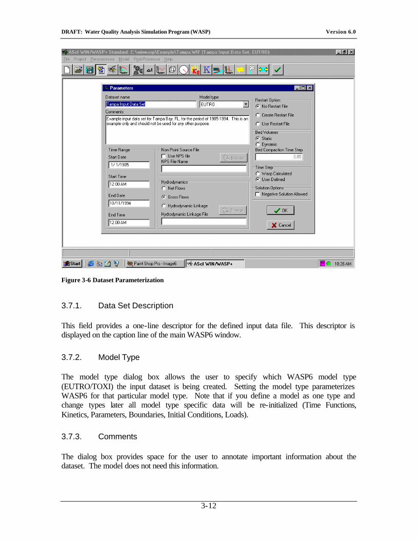
Figure 3-6 Dataset Parameterization
3.7.1. Data Set Description
This field provides a one-line descriptor for the defined input data file. This descriptor is displayed on the caption line of the main WASP6 window.
3.7.2. Model Type
The model type dialog box allows the user to specify which WASP6 model type (EUTRO/TOXI) the input dataset is being created. Setting the model type parameterizes WASP6 for that particular model type. Note that if you define a model as one type and change types later all model type specific data will be re-initialized (Time Functions, Kinetics, Parameters, Boundaries, Initial Conditions, Loads).
3.7.3. Comments
The dialog box provides space for the user to annotate important information about the dataset. The model does not need this information.
DRAFT: Water Quality Analysis Simulation Program (WASP) Version 6.0
3-13
3.7.4. Restart Options
WASP6 provides the user with the ability to use restart files between simulation runs. A restart file is a “snap-shot” of the model conditions at the end of the simulation. This “snap-shot” can be used as the initial conditions for a future model run. Note that the future model run must be of the same model type and segmentation scheme. There are three options for Restart:
1. No Restart File – WASP6 does not create a restart file (default).
2. Create Restart File – WASP6 creates a restart file that contains the final volumes and concentrations for each of the segments and systems.
3. Create/Read Restart File – WASP6 creates a file as described above, but reads initial volumes and concentrations from a previously created restart file.
3.7.5. Date and Times
The previous versions of WASP did not require that the model time functions be represented in Gregorian date format. The Version 6.0of WASP requires all time functions be represented in Gregorian fashion (mm/dd/yr hh:mm:ss). The user in the Start Time dialog box must specify the starting date and time. This date and time correspond to time zero in the old version of the model.
3.7.6. Non-Point Source File
The non-point source file is an external file that contains a time-series of loads (kg/day) for a given segment and system. This file is typically created either by the user manually or using other software like the Stormwater Management Model (SWMM) in conjunction with the Linked Watershed/Waterbody Model. This file can be used to provide loading information to WASP6 on virtually any time scale, from timestep to timestep, to year average loads.
3.7.7. Hydrodynamics
There are currently three surface flow options available for WASP. The first two options pertain to how WASP will calculate the exchange of mass between adjoining segments with flow in both directions across a segment interface. The three flow options available for surface water flow are:
1. WASP will calculate net transport across a segment interface that has opposing flow. WASP will net the flows and move the mass from the segment that has the higher flow leaving. If the opposed flows are equal no mass is moved.
2. Pertains to mass and water being moved without regard to net flow.
DRAFT: Water Quality Analysis Simulation Program (WASP) Version 6.0
3-14
3. This option is used when linking WASP to a hydrodynamic model. When option 3 is selected the user cannot provide any additional surface flow information. Upon execution of a WASP input dataset using option 3 the hydrodynamic linkage file must already be created and exist in the directory that the input dataset resides. The file must have the extension of *.HYD.
The hydrodynamic linkage dialog box allows the user to select a hydrodynamic linkage file. The hydrodynamic linkage file provides flows, volumes, depths, and velocities to the WASP6 model during execution. There are several hydrodynamic models that have been linked with WASP6. The models include: DYNHYD5, RIVMOD, EFDC and SWMM's transport module.
When linking to a hydrodynamic interface file, the user is restrained from entering additional surface flow information.
3.8. Systems
The system data entry form allows the user to define system specific information. A system in WASP6 is a state variable within the model. The state variables in WASP6 change from one model type to another. The user controls, which state variables, will be considered in their model input dataset from within this screen.
DRAFT: Water Quality Analysis Simulation Program (WASP) Version 6.0
3-15
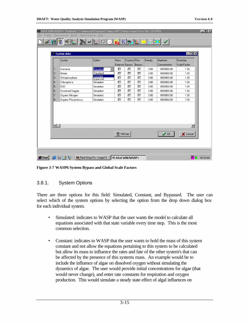
Figure 3-7 WASP6 System Bypass and Global Scale Factors
3.8.1. System Options
There are three options for this field: Simulated, Constant, and Bypassed. The user can select which of the system options by selecting the option from the drop down dialog box for each individual system.
• Simulated: indicates to WASP that the user wants the model to calculate all equations associated with that state variable every time step. This is the most common selection.
• Constant: indicates to WASP that the user wants to hold the mass of this system constant and not allow the equations pertaining to this system to be calculated but allow its mass to influence the rates and fate of the other system's that can be affected by the presence of this systems mass. An example would be to include the influence of algae on dissolved oxygen without simulating the dynamics of algae. The user would provide initial concentrations for algae (that would never change), and enter rate constants for respiration and oxygen production. This would simulate a steady state effect of algal influences on
DRAFT: Water Quality Analysis Simulation Program (WASP) Version 6.0
3-16
dissolved oxygen without providing all the information needed to simulate algae.
• Bypassed: indicates to WASP that NO calculations should be done for the particular system. When a system is bypassed in WASP the user does not have to provide boundary concentrations or initial conditions. When bypassing systems in WASP make sure that you are not removing an integral part of the problem you are trying to solve.
For both the advective and dispersive transport functions in WASP, the user has the ability to bypass the effect of the particular transport phenomenon on the particular state variable in WASP. If the user would like to see the effect of algae on the system when it is not allowed to transport, the user sets the bypass flag for Chlorophyll-a to "Y" in either advection or dispersion (possibly both)
3.8.2. Dispersion/Flow Bypass
The dispersion/flow bypass option allows the user to specify whether a state variable will transport by either one of these processes. If the user did not want a state variable to be affected by dispersion or flow they should check the appropriate box.
3.8.3. Density
The density of each constituent must be specified under initial conditions as well (g/cm3).
3.8.4. Maximum Concentration
The maximum concentration column allows the user to specify what would be the expected maximum concentration (mg/l) of any of the given state variables. If WASP6 predicted a concentration greater than the supplied value here the model simulation would be terminated.
3.8.5. Boundary/Load Scale & Conversion Factor
The boundary scale and conversion factors are specified for each individual system. The conversion factor can be used for converting the boundary time series information to the appropriate concentration units used by WASP6. The scale factor can be used to attenuate the boundary concentrations without re-entering the time series data. An example would be if the user wanted to know what the effects of doubling the loads would be on water quality. Instead of re-entering the time series data, setting the scale factor to 2 would cause WASP6 to multiple the times series by 2.

DRAFT: Water Quality Analysis Simulation Program (WASP) Version 6.0
3-17
3.9. Segmentation Screen
This data entry form allows the user to define the number of segments that will be considered in the simulation. Segments are the spatial component in which WASP6 solves it’s set of equations. Segments have volume, environmental and constituent concentrations associated with them. The segment data entry form has four tables associated with them: 1) Segment Definition, 2) Environmental Parameters, 3) Initial Conditions, 4) Fraction Dissolved.
3.9.1. Segment Definition
The segment definition screen is where the user provides segment specific geometry information. It is import that the user has a good understanding in how their water body will be segmented prior to entering the information on this screen.
Figure 3-8 Segment Definitions
Inserting/Deleting Segments
Before the user can define a segment, the user needs to insert a segment by clicking on the insert button. This will cause a segment to be inserted at the active row in the table.
DRAFT: Water Quality Analysis Simulation Program (WASP) Version 6.0
3-18
If this is the first segment to be inserted it will initiate the table and insert a row at the top.
To delete a segment, highlight the row in which you want to delete and click on the delete button.
Segment Naming Convention
WASP6 automatically names the segments by numbers 1 through the number of segments. WASP6 also allows the user to give an alphanumeric name to individual segments. This alphanumeric name is there for the convenience of the user and will appear on the other screens (Dispersion, Flow) as well as in the post processor so that the user does not need to keep track of the segments by number alone. When you initially insert a segment it is automatically given the name WASP Segment. To name segments highlight the cell and type the name for each segment.
Volumes
This column represents the volume of the segment that is being defined. The units for volume are cubic meters. Note that WASP6 does not assume a cubic formation for a segment, the shape is arbitrary.
Water Velocity/Depth
There are several options for specifying water velocity and depth to WASP6. Depth and velocity can be held constant by entering their values in the Depth and Velocity multiplier field and setting the exponent to zero. The user may also allow depth and velocity to vary as a function of flow. To do this the user must provide a depth and velocity multiplier and exponent. The velocity (m/s) is computed from the formulation aQb while the depth (m) is computed from cQd, where a & d are coefficients and Q is the flow (m3/sec).
Segment Type
WASP6 supports four different segment types. The user must provide a segment type for each of the segments being defined. The segment type dialog box is used to define the segment type for the segment being defined.
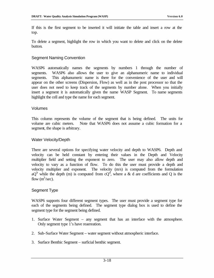
1. Surface Water Segment – any segment that has an interface with the atmosphere. Only segment type 1’s have reaereation.
2. Sub-Surface Water Segment – water segment without atmospheric interface.
3. Surface Benthic Segment – surficial benthic segment.
DRAFT: Water Quality Analysis Simulation Program (WASP) Version 6.0
3-19
4. Sub-Surface Benthic Segment – all benthic segments below surface benthic segments.
Bottom Segment
The bottom segment is used to define which segment is below the currently being defined segment. If the segment does not have a segment below it, the bottom segment should be set to none or zero. The bottom segment definition is used to define the optical light path; it is not used in transport calculations.
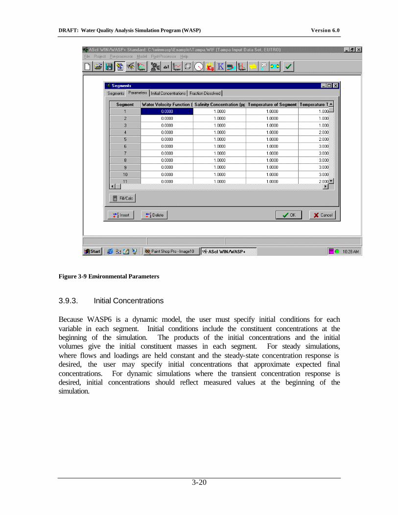
3.9.2. Segment Environmental Parameters
This table contains segment specific environmental parameters. These parameters are different for the various WASP6 model types. The segment parameter information interacts directly with the Parameter Scale Factor screen.
The user only needs to provide information for the environmental parameters that are going to be considered in the simulation. Some parameters are used to directly define segment specific information (i.e. SOD), others are used to point to environmental time functions (i.e. Temperature). The pointers to environmental time functions allow the user to define spatial and temporal variation for segment parameters such as: temperature, water velocity, pH, and bacteria concentration.
DRAFT: Water Quality Analysis Simulation Program (WASP) Version 6.0
3-20
Figure 3-9 Environmental Parameters
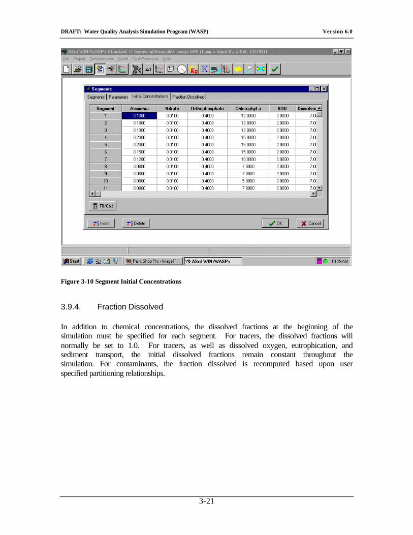
3.9.3. Initial Concentrations
Because WASP6 is a dynamic model, the user must specify initial conditions for each variable in each segment. Initial conditions include the constituent concentrations at the beginning of the simulation. The products of the initial concentrations and the initial volumes give the initial constituent masses in each segment. For steady simulations, where flows and loadings are held constant and the steady-state concentration response is desired, the user may specify initial concentrations that approximate expected final concentrations. For dynamic simulations where the transient concentration response is desired, initial concentrations should reflect measured values at the beginning of the simulation.
DRAFT: Water Quality Analysis Simulation Program (WASP) Version 6.0
3-21
Figure 3-10 Segment Initial Concentrations
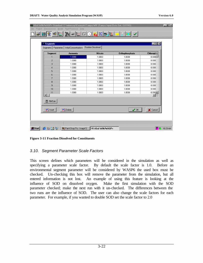
3.9.4. Fraction Dissolved
In addition to chemical concentrations, the dissolved fractions at the beginning of the simulation must be specified for each segment. For tracers, the dissolved fractions will normally be set to 1.0. For tracers, as well as dissolved oxygen, eutrophication, and sediment transport, the initial dissolved fractions remain constant throughout the simulation. For contaminants, the fraction dissolved is recomputed based upon user specified partitioning relationships.
DRAFT: Water Quality Analysis Simulation Program (WASP) Version 6.0
3-22
Figure 3-11 Fraction Dissolved for Constituents
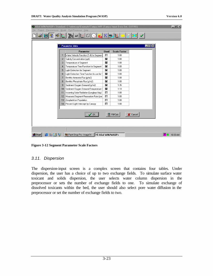
3.10. Segment Parameter Scale Factors
This screen defines which parameters will be considered in the simulation as well as specifying a parameter scale factor. By default the scale factor is 1.0. Before an environmental segment parameter will be considered by WASP6 the used box must be checked. Un-checking this box will remove the parameter from the simulation, but all entered information is not lost. An example of using this feature is looking at the influence of SOD on dissolved oxygen. Make the first simulation with the SOD parameter checked; make the next run with it un-checked. The differences between the two runs are the influence of SOD. The user can also change the scale factors for each parameter. For example, if you wanted to double SOD set the scale factor to 2.0
DRAFT: Water Quality Analysis Simulation Program (WASP) Version 6.0
3-23
Figure 3-12 Segment Parameter Scale Factors
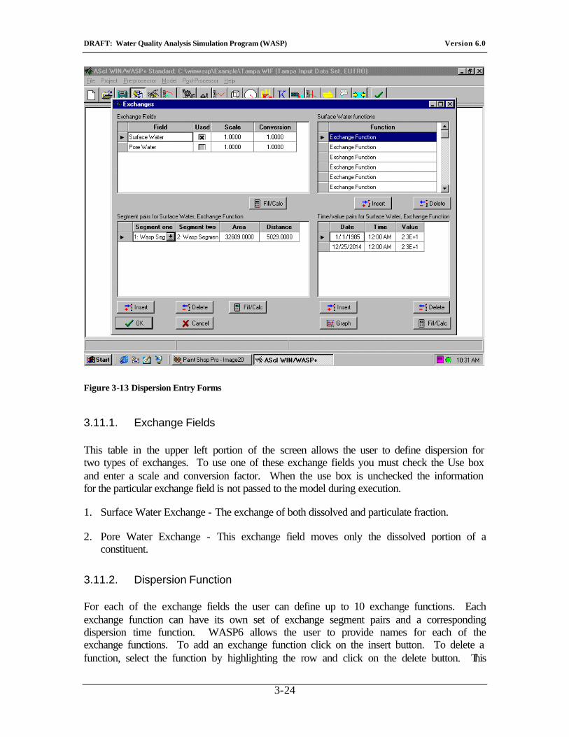
3.11. Dispersion
The dispersion-input screen is a complex screen that contains four tables. Under dispersion, the user has a choice of up to two exchange fields. To simulate surface water toxicant and solids dispersion, the user selects water column dispersion in the preprocessor or sets the number of exchange fields to one. To simulate exchange of dissolved toxicants within the bed, the user should also select pore water diffusion in the preprocessor or set the number of exchange fields to two.
DRAFT: Water Quality Analysis Simulation Program (WASP) Version 6.0
3-24
Figure 3-13 Dispersion Entry Forms
3.11.1. Exchange Fields
This table in the upper left portion of the screen allows the user to define dispersion for two types of exchanges. To use one of these exchange fields you must check the Use box and enter a scale and conversion factor. When the use box is unchecked the information for the particular exchange field is not passed to the model during execution.
1. Surface Water Exchange - The exchange of both dissolved and particulate fraction.
2. Pore Water Exchange - This exchange field moves only the dissolved portion of a constituent.
3.11.2. Dispersion Function
For each of the exchange fields the user can define up to 10 exchange functions. Each exchange function can have its own set of exchange segment pairs and a corresponding dispersion time function. WASP6 allows the user to provide names for each of the exchange functions. To add an exchange function click on the insert button. To delete a function, select the function by highlighting the row and click on the delete button. This
DRAFT: Water Quality Analysis Simulation Program (WASP) Version 6.0
3-25
will delete the corresponding segment pairs (lower left table) and the dispersion time function (lower right table).
To insert exchange functions for surface dispersion, highlight the Surface dispersion exchange field (upper left table) go over to the exchange function table (upper right table) and press insert. The bottom tables are a function of the selection in the upper tables.
Segment Pairs
The segment pairs define the between which an exchange will occur. It does not matter in which order they are defined. Neither the preprocessor, nor the model makes any checks to make sure the segments are connected in any manner. Connectivity is the responsibility of the user.
Cross Sectional Area
Cross-sectional areas are specified for each dispersion coefficient, reflecting the area through which mixing occurs. These can be surface areas for vertical exchange, such as in lakes or in the benthos. Areas are not modified during the simulation to reflect flow changes.
Characteristic Mixing Length
Mixing lengths or distance are specified for each dispersion coefficient, reflecting the characteristic length over which mixing occurs. These are typically the lengths between the center points of adjoining segments. A single segment may have three or more mixing lengths for segments adjoining longitudinally, laterally, and vertically. For surficial benthic segments connecting water column segments, the depth of the benthic layer is a more realistic mixing length than half the water depth.
3.11.3. Dispersion Time Function
Dispersive mixing coefficients can be specified between adjoining segments, or across open water boundaries. These coefficients may represent pore water diffusion in benthic segments, vertical diffusion in lakes, and lateral and longitudinal dispersion in large water bodies. Values can range from 1x10⁻¹⁰ m2/sec for molecular diffusion to 5x10² m2/sec for longitudinal mixing in some estuaries. Values are entered as a time function series of dispersion and time, in days.
3.12. Flows
The flow groups works exactly the same way as the exchange group. The only difference is that the advective group has 6 transport processes that can be defined by the user.
DRAFT: Water Quality Analysis Simulation Program (WASP) Version 6.0
3-26
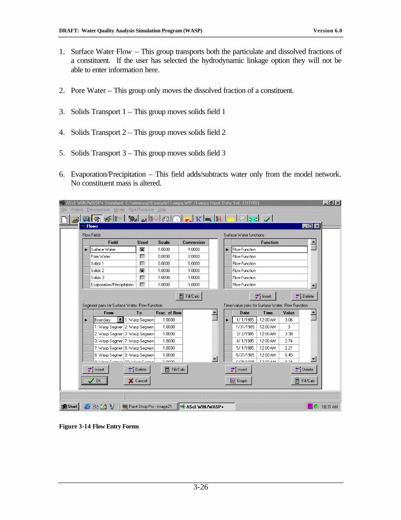
1. Surface Water Flow – This group transports both the particulate and dissolved fractions of a constituent. If the user has selected the hydrodynamic linkage option they will not be able to enter information here.
2. Pore Water – This group only moves the dissolved fraction of a constituent.
3. Solids Transport 1 – This group moves solids field 1
4. Solids Transport 2 – This group moves solids field 2
5. Solids Transport 3 – This group moves solids field 3
6. Evaporation/Precipitation – This field adds/subtracts water only from the model network. No constituent mass is altered.
Figure 3-14 Flow Entry Forms
DRAFT: Water Quality Analysis Simulation Program (WASP) Version 6.0
3-27
3.12.1. Flow Function
The user has the ability to define 10 flow functions for each of the six flow fields. Each flow function would have its own flow continuity input (lower left table) and time variable flow input (lower right table). The user must highlight the flow field and flow function in which to enter information. WASP6 allows the user to provide names for each of the flow functions. To insert an exchange function click on the insert button. To delete a function, select the function by highlighting the row and click on the delete button. Note: this will delete the corresponding segment pairs (lower left table) and the flow time function (lower right table).
To insert flow functions for surface flow, highlight the Surface Flow field (upper left table) go over to the flow function table (upper right table) and press insert. The bottom tables are a function of the selection in the upper tables.
Segment Pairs
The segment pairs define the segments from/to, which flow, occurs. The order in which the segment is defined should be the path of positive flow. In other words, if segment 1 flows to segment 2, when a negative flow is entered in the time function the flow will be from 2 to 1. Note: Neither preprocessor, nor the model makes any checks to make sure the segments are connected in any manner. Connectivity is the responsibility of the user.
Fraction of Flow
The fraction of flow column allows the user to specify the fraction of the flow that transports from one to segment to the other. This field is used to split flows (diverge) for various reasons.
3.12.2. Flow Time Function
The time function table allows the user to enter time variable flow information. The user must provide the date, time and flow (cms).
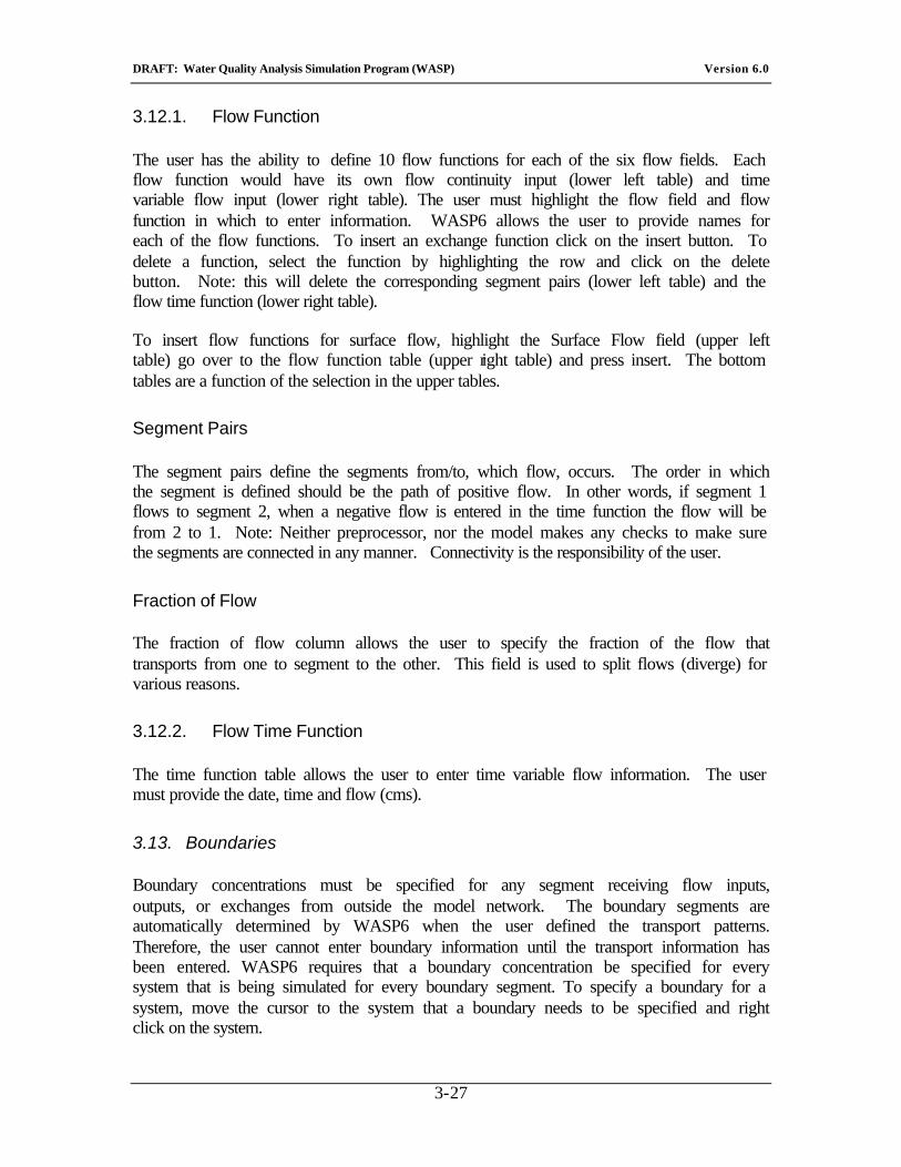
3.13. Boundaries
Boundary concentrations must be specified for any segment receiving flow inputs, outputs, or exchanges from outside the model network. The boundary segments are automatically determined by WASP6 when the user defined the transport patterns. Therefore, the user cannot enter boundary information until the transport information has been entered. WASP6 requires that a boundary concentration be specified for every system that is being simulated for every boundary segment. To specify a boundary for a system, move the cursor to the system that a boundary needs to be specified and right click on the system.
DRAFT: Water Quality Analysis Simulation Program (WASP) Version 6.0
3-28
Figure 3-15 Boundary Concentration Definitions
3.13.1. Boundary Time Function
The time function table allows the user to enter time variable boundary concentrations (mg/l). The user must provide the date, time and concentration.
Note: For chlorophyll-a boundary conditions the units are ög/l
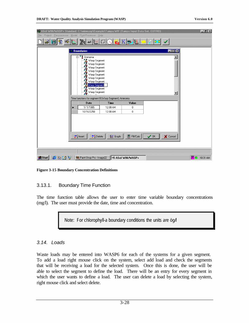
3.14. Loads
Waste loads may be entered into WASP6 for each of the systems for a given segment. To add a load right mouse click on the system, select add load and check the segments that will be receiving a load for the selected system. Once this is done, the user will be able to select the segment to define the load. There will be an entry for every segment in which the user wants to define a load. The user can delete a load by selecting the system, right mouse click and select delete.
DRAFT: Water Quality Analysis Simulation Program (WASP) Version 6.0
3-29
Figure 3-16 Waste Load Definition Screen
3.14.1. Load Time Function
The time function table allows the user to enter time variable loadings (kg/day). The user must provide the date, time and concentration.
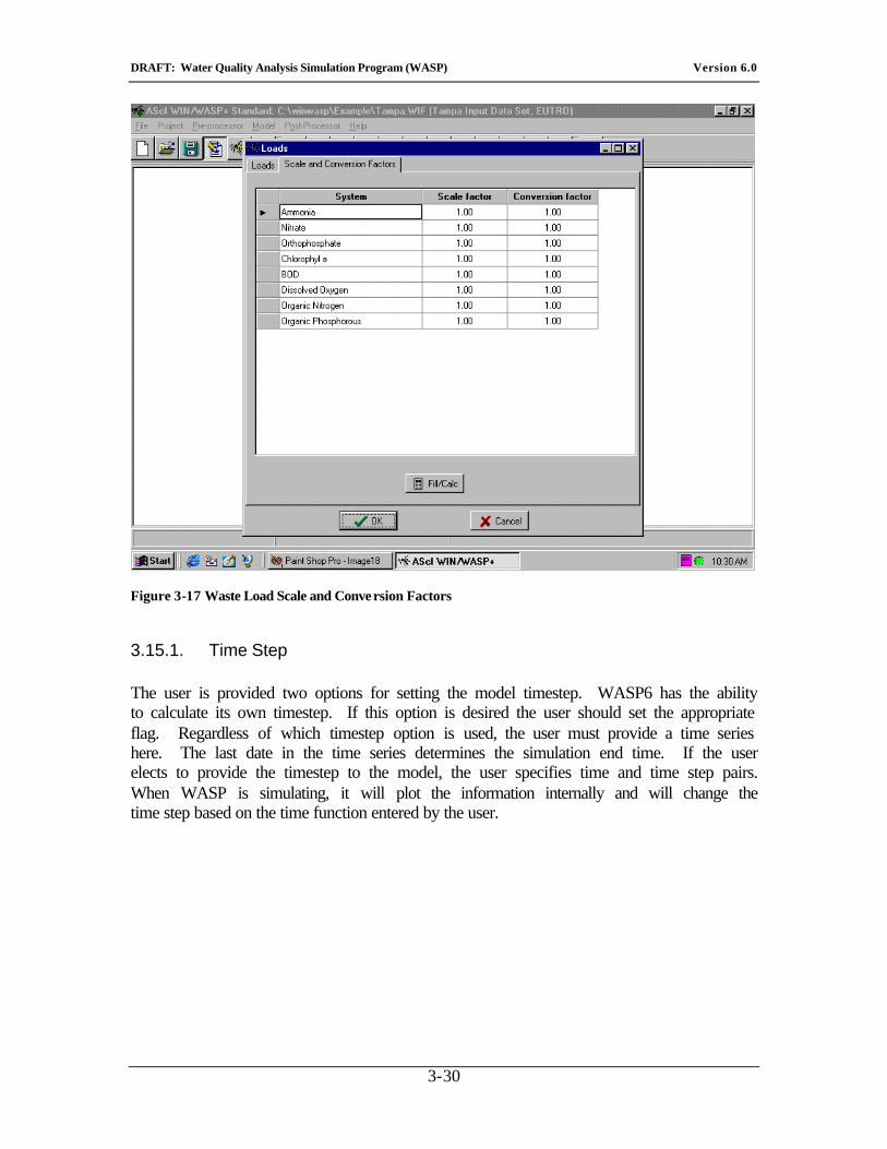
3.15. Loads Scale and Conversion
The user has the ability to provide scale and conversion factors that can be used to attenuate or convert loading mass. The conversion factor for a given system can be used to convert loads measured and reported in one unit to convert to WASP6 required units of kg/day. The scale factor column can be used to attenuate the loads without re-entering the time function information. If the user wanted to see the impacts of doubling the loads, a scale factor of 2 would be entered for the desired system.
DRAFT: Water Quality Analysis Simulation Program (WASP) Version 6.0
3-30
Figure 3-17 Waste Load Scale and Conve rsion Factors
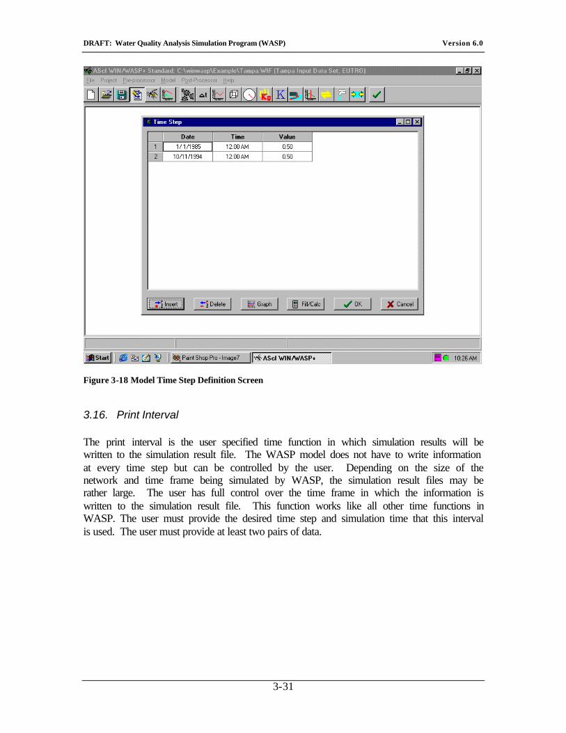
3.15.1. Time Step
The user is provided two options for setting the model timestep. WASP6 has the ability to calculate its own timestep. If this option is desired the user should set the appropriate flag. Regardless of which timestep option is used, the user must provide a time series here. The last date in the time series determines the simulation end time. If the user elects to provide the timestep to the model, the user specifies time and time step pairs. When WASP is simulating, it will plot the information internally and will change the time step based on the time function entered by the user.
DRAFT: Water Quality Analysis Simulation Program (WASP) Version 6.0
3-31
Figure 3-18 Model Time Step Definition Screen
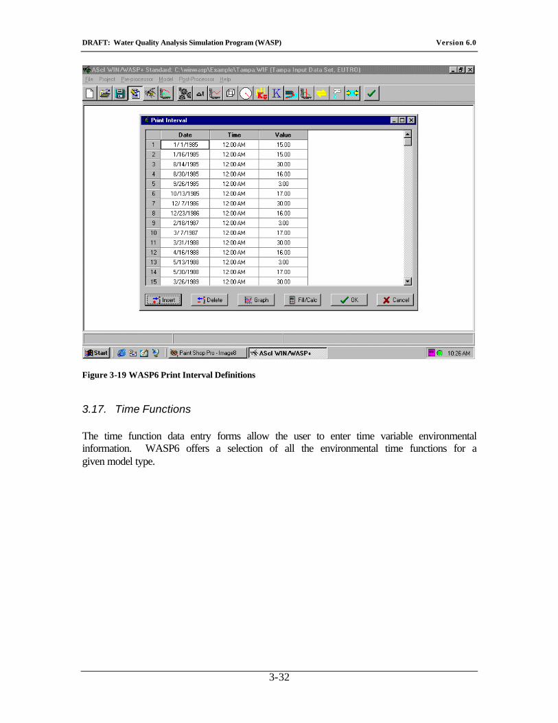
3.16. Print Interval
The print interval is the user specified time function in which simulation results will be written to the simulation result file. The WASP model does not have to write information at every time step but can be controlled by the user. Depending on the size of the network and time frame being simulated by WASP, the simulation result files may be rather large. The user has full control over the time frame in which the information is written to the simulation result file. This function works like all other time functions in WASP. The user must provide the desired time step and simulation time that this interval is used. The user must provide at least two pairs of data.
DRAFT: Water Quality Analysis Simulation Program (WASP) Version 6.0
3-32
Figure 3-19 WASP6 Print Interval Definitions
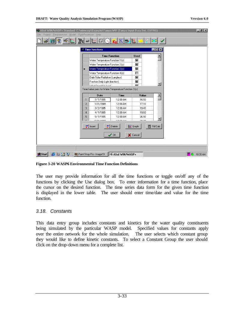
3.17. Time Functions
The time function data entry forms allow the user to enter time variable environmental information. WASP6 offers a selection of all the environmental time functions for a given model type.
DRAFT: Water Quality Analysis Simulation Program (WASP) Version 6.0
3-33
Figure 3-20 WASP6 Environmental Time Function Definitions
The user may provide information for all the time functions or toggle on/off any of the functions by clicking the Use dialog box. To enter information for a time function, place the cursor on the desired function. The time series data form for the given time function is displayed in the lower table. The user should enter time/date and value for the time function.
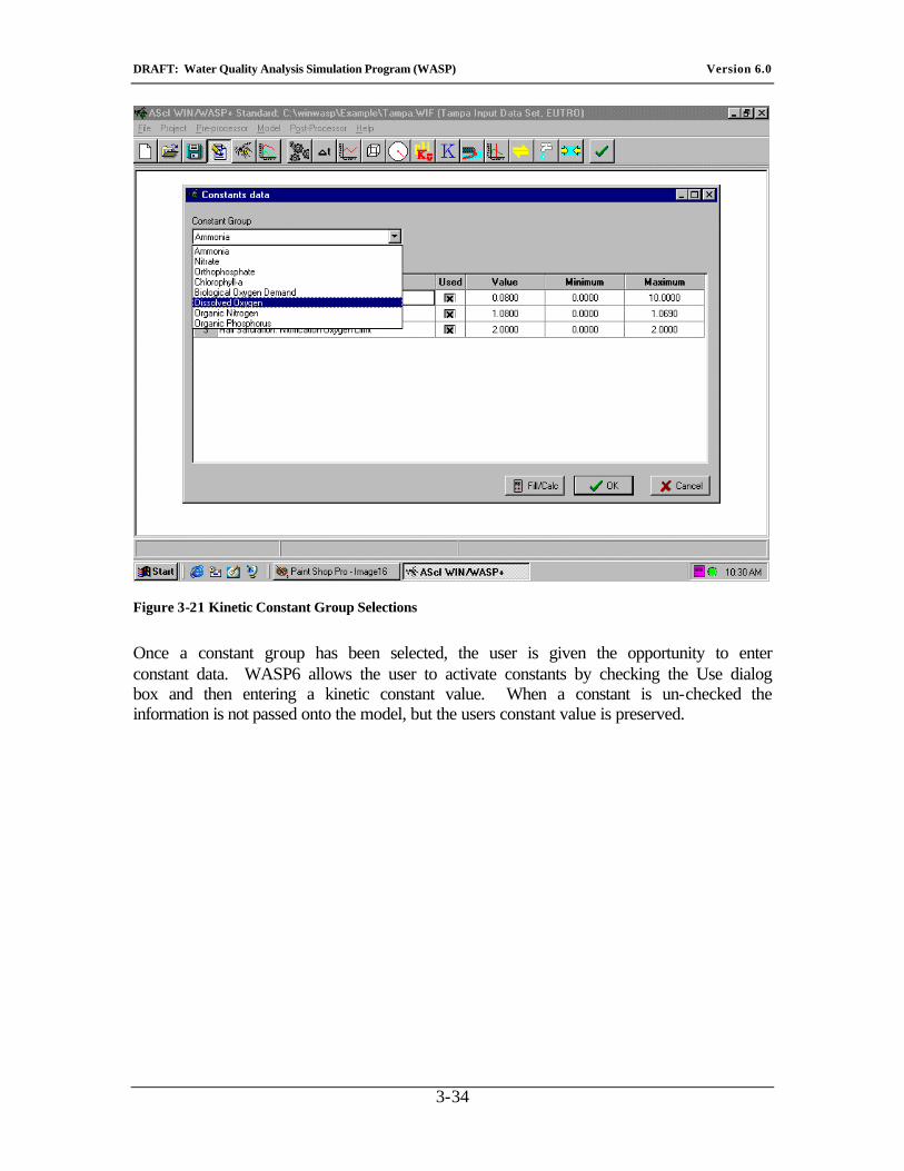
3.18. Constants
This data entry group includes constants and kinetics for the water quality constituents being simulated by the particular WASP model. Specified values for constants apply over the entire network for the whole simulation. The user selects which constant group they would like to define kinetic constants. To select a Constant Group the user should click on the drop-down menu for a complete list.
DRAFT: Water Quality Analysis Simulation Program (WASP) Version 6.0
3-34
Figure 3-21 Kinetic Constant Group Selections
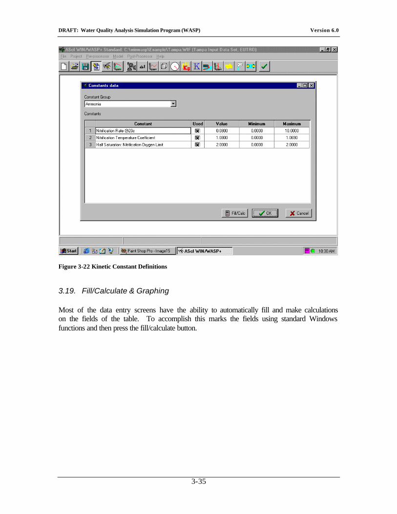
Once a constant group has been selected, the user is given the opportunity to enter constant data. WASP6 allows the user to activate constants by checking the Use dialog box and then entering a kinetic constant value. When a constant is un-checked the information is not passed onto the model, but the users constant value is preserved.
DRAFT: Water Quality Analysis Simulation Program (WASP) Version 6.0
3-35
Figure 3-22 Kinetic Constant Definitions
3.19. Fill/Calculate & Graphing
Most of the data entry screens have the ability to automatically fill and make calculations on the fields of the table. To accomplish this marks the fields using standard Windows functions and then press the fill/calculate button.
DRAFT: Water Quality Analysis Simulation Program (WASP) Version 6.0
3-36
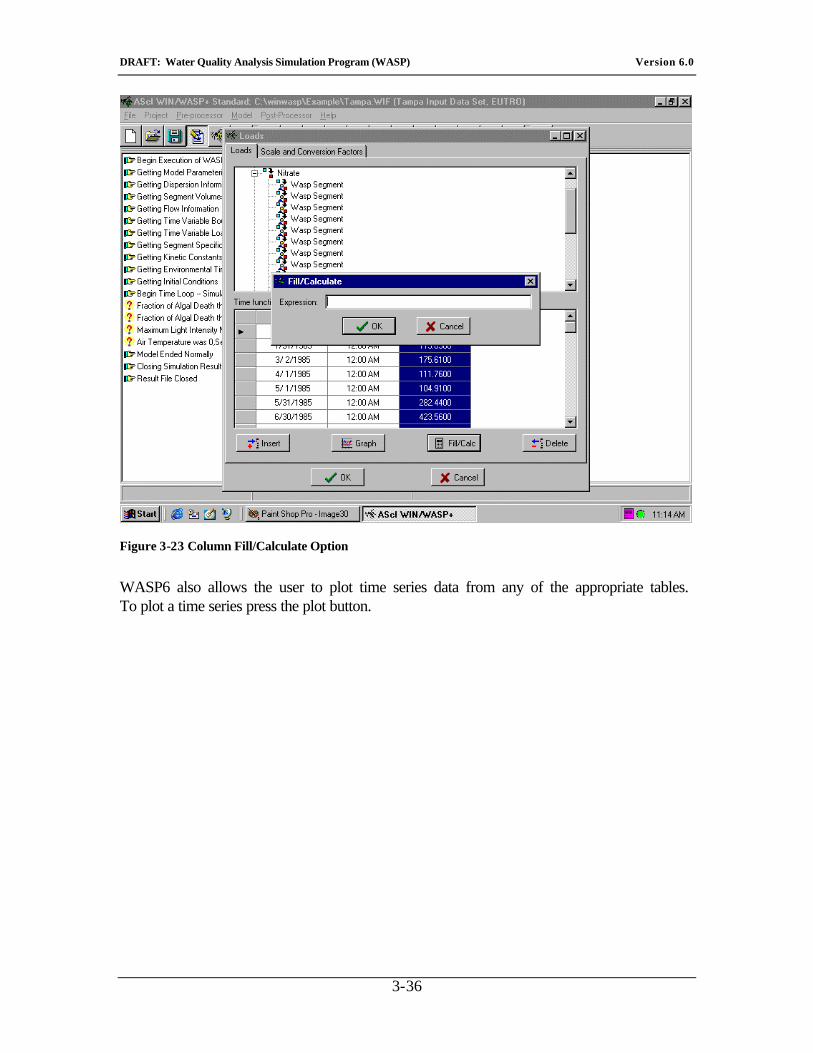
Figure 3-23 Column Fill/Calculate Option
WASP6 also allows the user to plot time series data from any of the appropriate tables. To plot a time series press the plot button.
DRAFT: Water Quality Analysis Simulation Program (WASP) Version 6.0
3-37
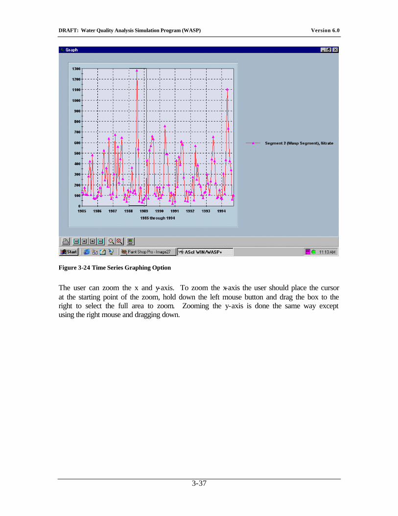
Figure 3-24 Time Series Graphing Option
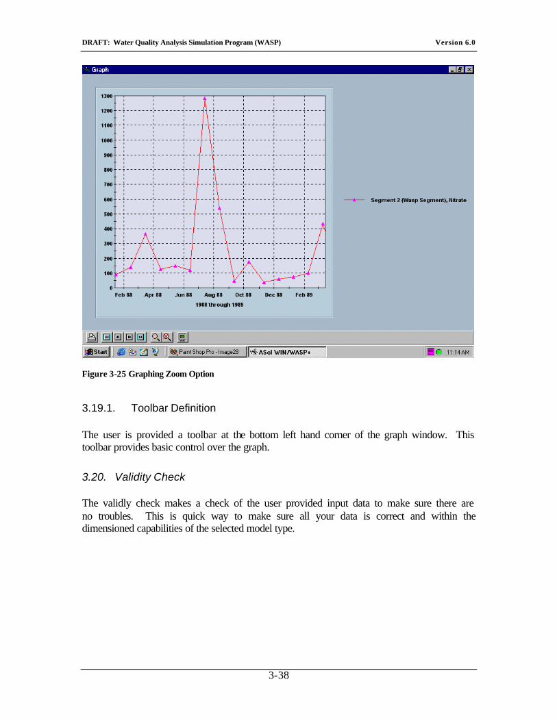
The user can zoom the x and y-axis. To zoom the x-axis the user should place the cursor at the starting point of the zoom, hold down the left mouse button and drag the box to the right to select the full area to zoom. Zooming the y-axis is done the same way except using the right mouse and dragging down.
DRAFT: Water Quality Analysis Simulation Program (WASP) Version 6.0
3-38
Figure 3-25 Graphing Zoom Option
3.19.1. Toolbar Definition
The user is provided a toolbar at the bottom left hand corner of the graph window. This toolbar provides basic control over the graph.
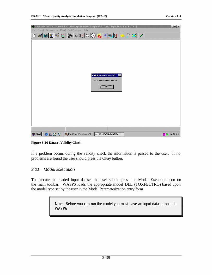
3.20. Validity Check
The validly check makes a check of the user provided input data to make sure there are no troubles. This is quick way to make sure all your data is correct and within the dimensioned capabilities of the selected model type.
DRAFT: Water Quality Analysis Simulation Program (WASP) Version 6.0
3-39
Figure 3-26 Dataset Validity Check
If a problem occurs during the validity check the information is passed to the user. If no problems are found the user should press the Okay button.
3.21. Model Execution
To execute the loaded input dataset the user should press the Model Execution icon on the main toolbar. WASP6 loads the appropriate model DLL (TOXI/EUTRO) based upon the model type set by the user in the Model Parameterization entry form.
Note: Before you can run the model you must have an input dataset open in WASP6
DRAFT: Water Quality Analysis Simulation Program (WASP) Version 6.0
3-40
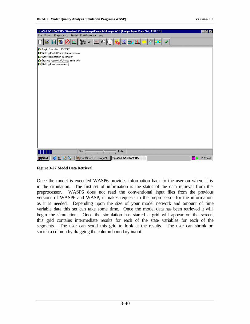
Figure 3-27 Model Data Retrieval
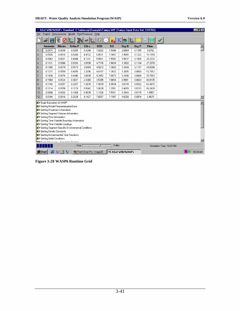
Once the model is executed WASP6 provides information back to the user on where it is in the simulation. The first set of information is the status of the data retrieval from the preprocessor. WASP6 does not read the conventional input files from the previous versions of WASP6 and WASP, it makes requests to the preprocessor for the information as it is needed. Depending upon the size of your model network and amount of time variable data this set can take some time. Once the model data has been retrieved it will begin the simulation. Once the simulation has started a grid will appear on the screen, this grid contains intermediate results for each of the state variables for each of the segments. The user can scroll this grid to look at the results. The user can shrink or stretch a column by dragging the column boundary in/out.
DRAFT: Water Quality Analysis Simulation Program (WASP) Version 6.0
3-41
Figure 3-28 WASP6 Runtime Grid
DRAFT: Water Quality Analysis Simulation Program (WASP) Version 6.0
4-42
4. Visual Graphic Post-Processor
The Post-Processor was developed as an efficient means of processing the vast amount of data produced by the execution of the WASP6 models. It has the ability to display results from all the models (EUTRO and TOXI) included in the WASP6 modeling package. The Post-Processor reads the output files created by the models and displays the results in two graphical formats:
1) Spatial Grid – a two dimensional rendition of the model network is displayed in a window where the model network is color shaded based upon the predicted concentration.
2) x/y Plots -- generates an x/y line plot of predicted and/or observed model results in a window.
There is no limit on the number of x/y plots, spatial grids or even model result files the user can utilize in a session. Separate windows are created for each spatial grid or x/y plot created by the user.
The Graphical Post-Processor is routinely executed from WASP6. Also, the user can use the Windows Explorer or Run button to execute the program. If executed from within WASP + with an input file selected, the corresponding model output files will be loaded. If executed from within WASP6 without an input file selected or by some other means, the user will need to use the file options for opening the files they want to display.
4.1. Main Toolbar
There are several toolbars and speed menus available. The main tool bar is available below the pull down menus provide the following functionality to the user. Depending upon the current status, some icons may not be available to perform a task, thus are not active.
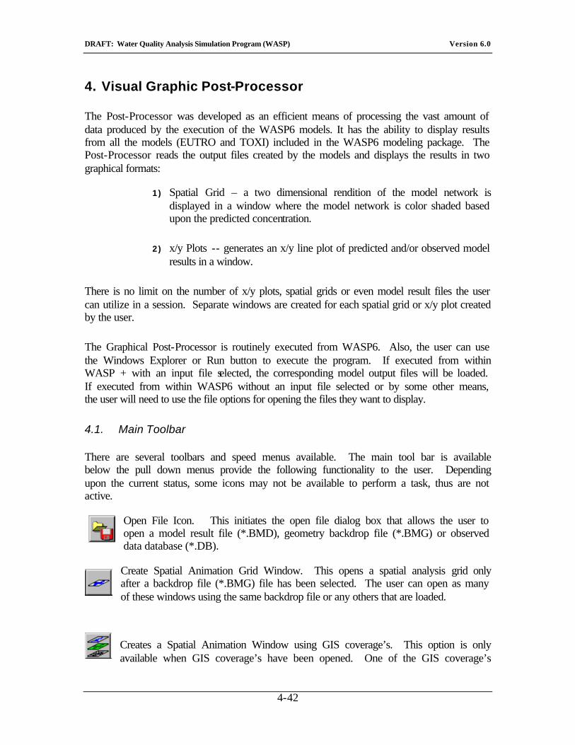
Open File Icon. This initiates the open file dialog box that allows the user to open a model result file (*.BMD), geometry backdrop file (*.BMG) or observed data database (*.DB).
Create Spatial Animation Grid Window. This opens a spatial analysis grid only after a backdrop file (*.BMG) file has been selected. The user can open as many of these windows using the same backdrop file or any others that are loaded.
Creates a Spatial Animation Window using GIS coverage’s. This option is only available when GIS coverage’s have been opened. One of the GIS coverage’s
DRAFT: Water Quality Analysis Simulation Program (WASP) Version 6.0
4-43
required is model network coverage.
Creates x/y plot Window. This opens an x/y plot window only after model data (*.BMD) or observed database data (*.DB) have been loaded. The user can open as many of these windows as desired to review any data that is loaded.
Edits the load observed data database
4.2. Model Output Selection
The Graphical Post-Processor was designed to allow the user to rapidly evaluate the results of the WASP model simulations and its support programs. Observed data can also be stored in a database format.
Four types of data are recognized:
� The first data type is created from the execution of the WASP models (*.BMD). The output from WASP is written in a binary file format. The model results cannot be read directly by any other program.
� The second file type that can be read is a Paradox table file (*.DB). The Paradox table file is used to provide observed/field data to be plotted against model predictions.
� The third file type is an ArcView shape file. These files can be used in the spatial analysis mode to aid the user in displaying the model network with respect to its geography and surrounding characteristics.
� The last file type that is used is the binary model geometry file. This file is used to provide the spatial grid geometry information so that the model results can be depicted within the model grid.
4.2.1. Opening Model Output
Prior to working with any model data or observed data, the files must be selected by the user. There is no limit to the number of files that can be opened. If the user would like to open additional files, the procedure given below will illustrate how to load each of the different file types. To open a file, the user can use the menu system and select open file or press the open file icon. This will display a file dialog box as illustrated in Figure 4-1. From this file dialog box the user can navigate to any drive and directory to which their computer is attached. By pressing the down arrow on the file type dialog, a list of valid file extensions is displayed for the user. Selecting an extension will result in the display of a picklist of the available files in the current drive and directory.
DRAFT: Water Quality Analysis Simulation Program (WASP) Version 6.0
4-44
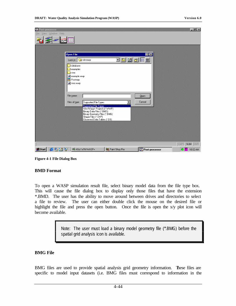
Figure 4-1 File Dialog Box
BMD Format
To open a WASP simulation result file, select binary model data from the file type box. This will cause the file dialog box to display only those files that have the extension *.BMD. The user has the ability to move around between drives and directories to select a file to review. The user can either double click the mouse on the desired file or highlight the file and press the open button. Once the file is open the x/y plot icon will become available.
Note: The user must load a binary model geometry file (*.BMG) before the spatial grid analysis icon is available.
BMG File
BMG files are used to provide spatial analysis grid geometry information. These files are specific to model input datasets (i.e. BMG files must correspond to information in the
DRAFT: Water Quality Analysis Simulation Program (WASP) Version 6.0
4-45
BMD files). BMG files are created using a utility program called Digitize. The file must be created prior to execution. The BMG file is selected in the same manner as the other files by setting the file type to BMG and selecting the file.
Note: The user must load a binary model geometry file (*.BMG) before the spatial grid analysis icon is available.
Observed Data
The observed data is in a Paradox 4.5 or higher format (*.DB). In order to display observed data versus the predicted model results, the database must be in a specific form. To load an observed data database follow the procedures described above, change the file type to *.DB. Select the database and press open.
Note: The "observed data" database is expected to be in a certain file format with pre-defined field names.
4.3. Spatial Graphical Analysis
The spatial graphical analysis allows the user to review model results for the whole network for a given constituent and time. This mode of graphical representation of the model results is very effective in illustrating model predictions to non-technical audiences.
4.3.1. Overview
The spatial graphical analysis function allows the user to illustrate the model results on a spatial grid using shading to represent predicted values. There are two options for creating spatial analysis grids. The first option allows the user to develop a binary model geometry file (*.BMG) to illustrate a portion of the modeling network or the complete network. The BMG is developed specifically for a particular model dataset with corresponding assignments for each of the model computational elements that are to be displayed. In other words, the BMG has polygons that are to be shaded based upon the predicted concentration of the model computational elements assigned to the polygons by the user at the time the BMG file is created.
The spatial grid analysis provides three modes for looking at the model results: shaded, wired frame, and violation/criteria shading. These various modes allows the spatial graphical analysis mode to illustrate information from model simulations in such a manner to make easier for the non-technical person to understand the results. The
DRAFT: Water Quality Analysis Simulation Program (WASP) Version 6.0
4-46
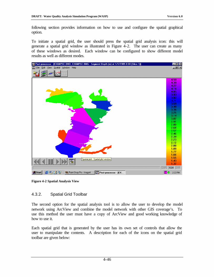
following section provides information on how to use and configure the spatial graphical option.
To initiate a spatial grid, the user should press the spatial grid analysis icon: this will generate a spatial grid window as illustrated in Figure 4-2. The user can create as many of these windows as desired. Each window can be configured to show different model results as well as different modes.
Figure 4-2 Spatial Analysis View
4.3.2. Spatial Grid Toolbar
The second option for the spatial analysis tool is to allow the user to develop the model network using ArcView and combine the model network with other GIS coverage’s. To use this method the user must have a copy of ArcView and good working knowledge of how to use it.
Each spatial grid that is generated by the user has its own set of controls that allow the user to manipulate the contents. A description for each of the icons on the spatial grid toolbar are given below:
DRAFT: Water Quality Analysis Simulation Program (WASP) Version 6.0
4-47
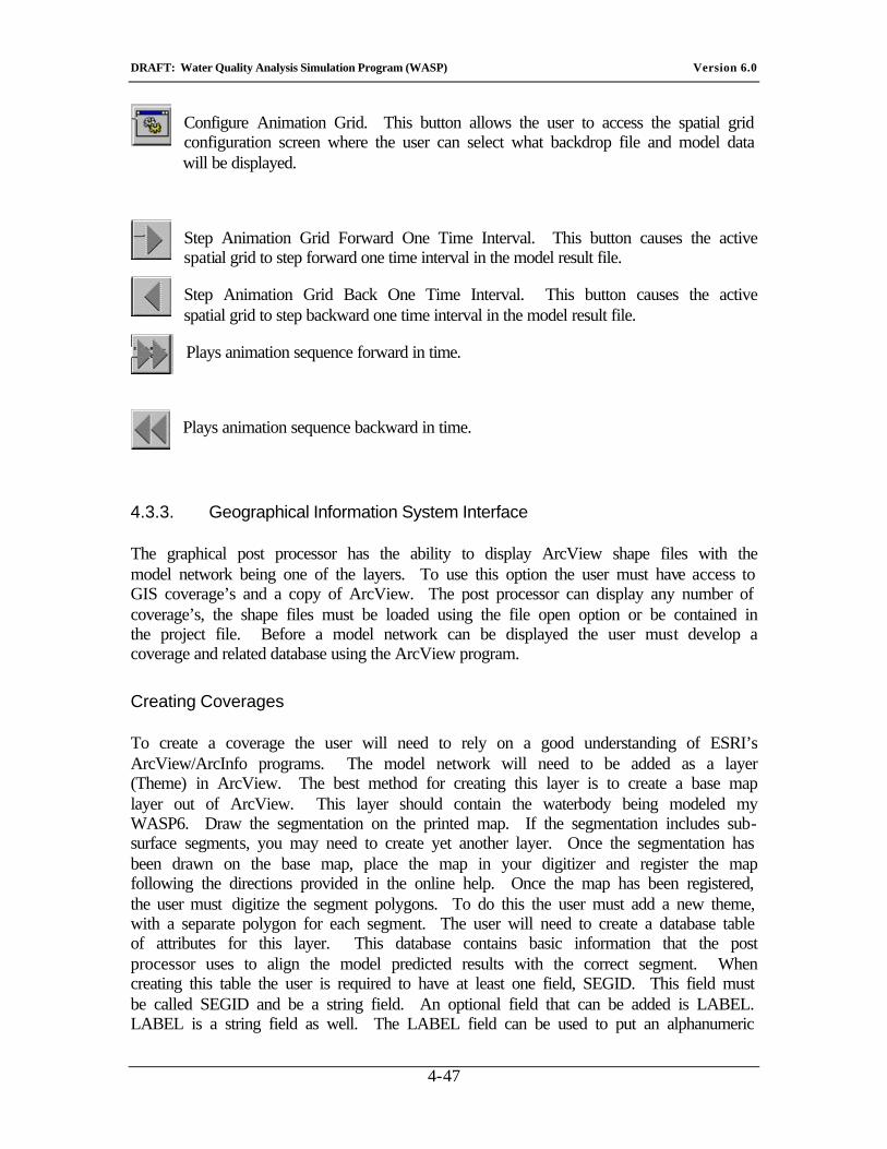
Configure Animation Grid. This button allows the user to access the spatial grid configuration screen where the user can select what backdrop file and model data will be displayed.
Step Animation Grid Forward One Time Interval. This button causes the active spatial grid to step forward one time interval in the model result file.
Step Animation Grid Back One Time Interval. This button causes the active spatial grid to step backward one time interval in the model result file.
Plays animation sequence forward in time.
Plays animation sequence backward in time.
4.3.3. Geographical Information System Interface
The graphical post processor has the ability to display ArcView shape files with the model network being one of the layers. To use this option the user must have access to GIS coverage’s and a copy of ArcView. The post processor can display any number of coverage’s, the shape files must be loaded using the file open option or be contained in the project file. Before a model network can be displayed the user must develop a coverage and related database using the ArcView program.
Creating Coverages
To create a coverage the user will need to rely on a good understanding of ESRI’s ArcView/ArcInfo programs. The model network will need to be added as a layer (Theme) in ArcView. The best method for creating this layer is to create a base map layer out of ArcView. This layer should contain the waterbody being modeled my WASP6. Draw the segmentation on the printed map. If the segmentation includes sub-surface segments, you may need to create yet another layer. Once the segmentation has been drawn on the base map, place the map in your digitizer and register the map following the directions provided in the online help. Once the map has been registered, the user must digitize the segment polygons. To do this the user must add a new theme, with a separate polygon for each segment. The user will need to create a database table of attributes for this layer. This database contains basic information that the post processor uses to align the model predicted results with the correct segment. When creating this table the user is required to have at least one field, SEGID. This field must be called SEGID and be a string field. An optional field that can be added is LABEL. LABEL is a string field as well. The LABEL field can be used to put an alphanumeric

DRAFT: Water Quality Analysis Simulation Program (WASP) Version 6.0
4-48
description next to the segment on the spatial plot. The user is referred to the ArcView documentation on how to create, edit and modify tables.
Figure 4-3 Model Database Definitions
4.3.4. BMG File Creation with Digitize
Before a spatial analysis grid can be displayed a BMG file needs to be created. This file is created using a utility program called Digitize. Digitize allows the user to draw the model network or the portion of the model network on the screen and assign cross section numbers to polygons that they represent. There is a one to one correspondence to polygons that are drawn with a cross section in the model BMD file.
Routine Execution of Digitize
The Digitize program is a DOS based program. Because Digitize needs access to the computers communication ports and uses its own communication drivers the program cannot be executed within the Windows environment. Digitize needs to be executed from the Windows Command Prompt option. To start Windows in the command prompt mode, restart your Windows system. When the Starting Windows string appears on the screen press the F8 key and select command prompt. To execute Digitize change directory to where the WASP6 modeling environment has been installed.
Digitize [parameters] digfile
The last step in creating the BMG file is linking all of the various slices into one BMG file. The BMG file is created using a program called Digilink.
DRAFT: Water Quality Analysis Simulation Program (WASP) Version 6.0
4-49
Developing a Spatial Grid
The spatial grid file (BMG) is a specially created file that provides geometric information. This geometric information is generated using the Digitize program. The Digitize program has two types of interfaces in which the user can enter the information: mouse and digitizer tablet. If the user has access to a digitizer this is probably the most advantageous mode for generating BMG files.
With Mouse
The mouse interface allows the user to develop the model grid by drawing the model network using the mouse. Each computational element being defined in the model network needs to be represented by an individual polygon. To use Digitize with the mouse interface the program needs to be loaded with the -m command line parameter. This instructs Digitize to get the drawing information from the mouse.
With Digitizer
The digitizer interface allows the user to develop the model grid by actually rendering the model network using a digitizer tablet. This is probably a more exact way of developing the model spatial grid. The digitizer interface allows the user to take engineering drawings of the waterbody and lay the model network right on top. When using the digitizer interface the user needs to instruct Digitize as to the communication port from which to read the information. This is done by using a command line parameter -COM2, which instructs Digitize to get the information from the digitizer tablet from communication port 2.
4.3.5. Controlling Spatial Analysis
Each of the spatial grid analysis windows can be configured several different ways to display the model results. The user can elect to display results in one of three animation modes:
1) Time – this mode animates the results for a single variable forward/backward in time. This is the preferred mode of the spatial analysis grid.
2) Variable – this displays the shaded results for each of the variables in the model output file. Pressing the forward/backward icon will cause the spatial animation grid to display the results for each of the variables.
3) Slice – this option displays the results for a given variable over the range of slices views found in the BMG file.
Figure 4-4 illustrates the configuration screen for the spatial analysis grid non-GIS.
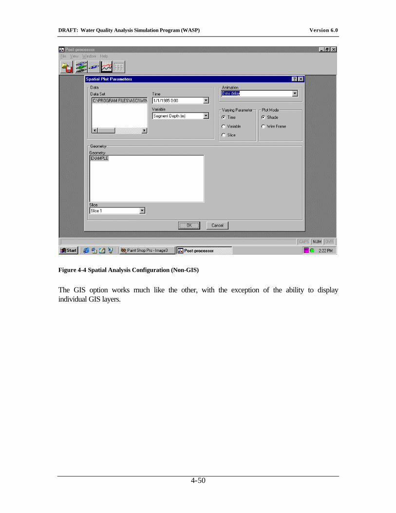
DRAFT: Water Quality Analysis Simulation Program (WASP) Version 6.0
4-50
Figure 4-4 Spatial Analysis Configuration (Non-GIS)
The GIS option works much like the other, with the exception of the ability to display individual GIS layers.
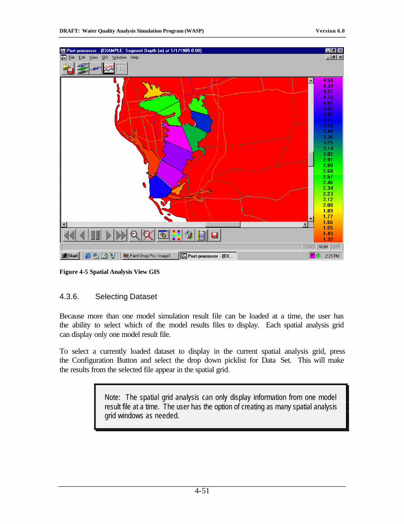
DRAFT: Water Quality Analysis Simulation Program (WASP) Version 6.0
4-51
Figure 4-5 Spatial Analysis View GIS
4.3.6. Selecting Dataset
Because more than one model simulation result file can be loaded at a time, the user has the ability to select which of the model results files to display. Each spatial analysis grid can display only one model result file.
To select a currently loaded dataset to display in the current spatial analysis grid, press the Configuration Button and select the drop down picklist for Data Set. This will make the results from the selected file appear in the spatial grid.
Note: The spatial grid analysis can only display information from one model result file at a time. The user has the option of creating as many spatial analysis grid windows as needed.
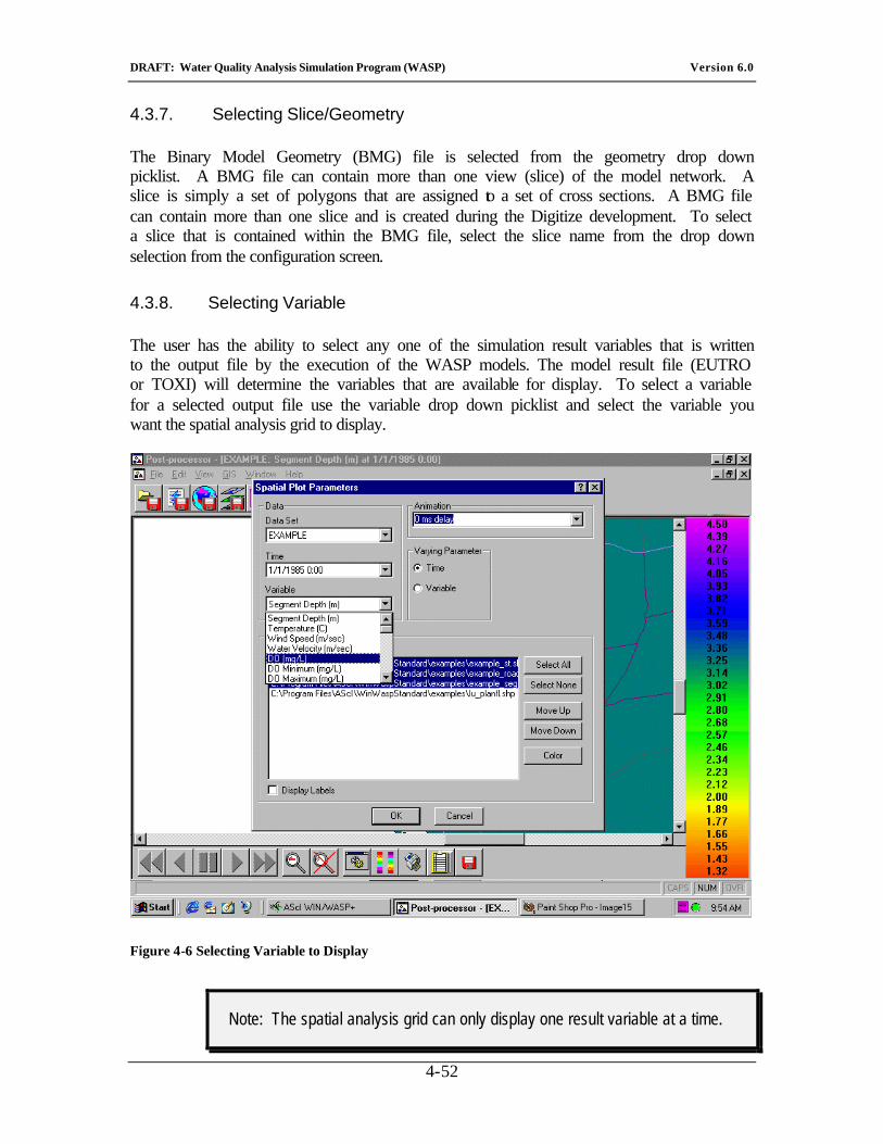
DRAFT: Water Quality Analysis Simulation Program (WASP) Version 6.0
4-52
4.3.7. Selecting Slice/Geometry
The Binary Model Geometry (BMG) file is selected from the geometry drop down picklist. A BMG file can contain more than one view (slice) of the model network. A slice is simply a set of polygons that are assigned to a set of cross sections. A BMG file can contain more than one slice and is created during the Digitize development. To select a slice that is contained within the BMG file, select the slice name from the drop down selection from the configuration screen.
4.3.8. Selecting Variable
The user has the ability to select any one of the simulation result variables that is written to the output file by the execution of the WASP models. The model result file (EUTRO or TOXI) will determine the variables that are available for display. To select a variable for a selected output file use the variable drop down picklist and select the variable you want the spatial analysis grid to display.
Figure 4-6 Selecting Variable to Display
Note: The spatial analysis grid can only display one result variable at a time.
DRAFT: Water Quality Analysis Simulation Program (WASP) Version 6.0
4-53
4.3.9. Selecting Time
The spatial analysis grid displays results for a given variable at a given time. Not only does the user have the ability to control the display of variables, but can control the display time as well. The user can select what simulation time to display the results for a given variable. This pull down picklist allows the user to move the spatial analysis grid to specific points in time without stepping through each time interval.
4.3.10. Palette
The user has the ability to modify the color palette that is used to shade the plot. The most common modification to the color palette would be to invert the currently loaded palette. Clicking on the Invert radio button will cause the color palette to be inverted (i.e. the colors for the lower values will become the colors for the higher values).
The user also has the ability to select a different color scheme by selecting a new palette. To select a new palette the user should press the browse button and select a palette.
4.3.11. Animation
The most common use for the spatial analysis grid is to animate the model predictions. When the forward/backward buttons on the toolbar are pressed, the spatial analysis grid is updated with the next time or variable depending upon the varying parameter. By continually pressing the forward button the user can create “a movie” of the model-predicted results. Alternatively, the user may press the movie icon. The speed of the animation is controlled by the options under the spatial plot parameters.
4.3.12. Plot Mode
Three modes are provided by which data can be displayed in the spatial grid analysis window:
Shaded
This mode displays the simulation results by shading the model computational element based upon the predicted concentration. A color legend is displayed on the right hand side of the spatial analysis window, and the computational elements are shaded in accordance to the legend based upon the concentrations predicted by the model.
Wire Frame
The mode displays the simulation results in a wire frame. This mode differs from the shade mode in that the model computation elements are not filled with a color based upon
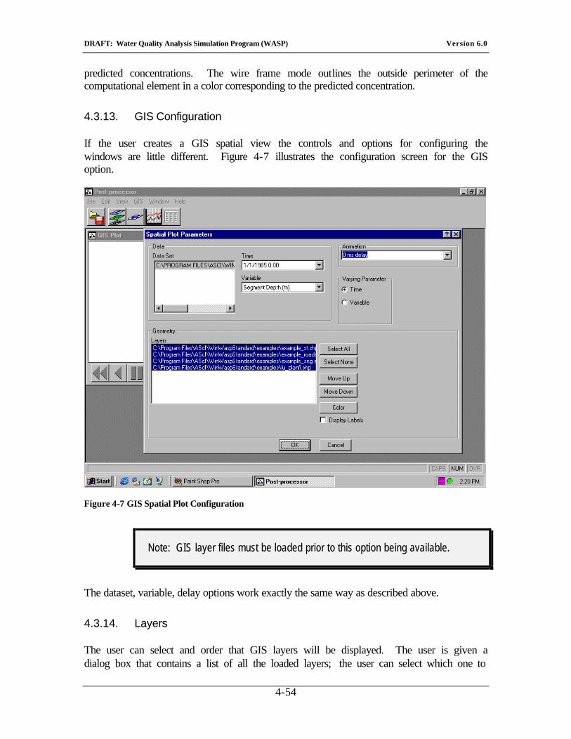
DRAFT: Water Quality Analysis Simulation Program (WASP) Version 6.0
4-54
predicted concentrations. The wire frame mode outlines the outside perimeter of the computational element in a color corresponding to the predicted concentration.
4.3.13. GIS Configuration
If the user creates a GIS spatial view the controls and options for configuring the windows are little different. Figure 4-7 illustrates the configuration screen for the GIS option.
Figure 4-7 GIS Spatial Plot Configuration
Note: GIS layer files must be loaded prior to this option being available.
The dataset, variable, delay options work exactly the same way as described above.
4.3.14. Layers
The user can select and order that GIS layers will be displayed. The user is given a dialog box that contains a list of all the loaded layers; the user can select which one to
DRAFT: Water Quality Analysis Simulation Program (WASP) Version 6.0
4-55
display by using standards Windows selection methods. Once a layer has been added to the selected dialog window, the user can control the order in which the layer is drawn by moving the layer up and down in the window. The model network should be the last layers to be drawn to make sure that another layer does not over write it.
Select All
This will select all of the loaded layers. Once they are selected the user should press the Add Button.
Select None
De-selects any selected layers.
Move Up/Down
The move/up down button will move the selected (highlighted) layer up in down in the list. The layers at the top of the list are drawn first.
Layer Color
The user has the ability select a specific color for a given layer. Because the GIS layers do not have a color associated, the post processor assigns a color. This assignment may not be desirable, to change the layer color select the layer and press the layer color button. The user will be presented a color selection dialog box. Select the color and press Okay.
4.3.15. GIS Toolbar
The GIS toolbar has a couple of additional buttons that are not found on non-GIS spatial analysis view.
This button will save the GIS view to a bitmap file. The user is presented a conventional file dialog box.
This copies the GIS view to the Windows Clipboard. Once in the clipboard it can be pasted into virtually another
Windows program.
This prints the GIS view to any printer connected to the system.
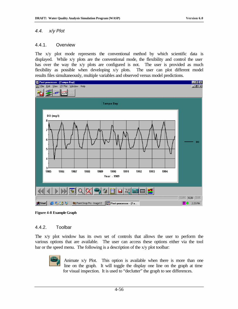
DRAFT: Water Quality Analysis Simulation Program (WASP) Version 6.0
4-56
4.4. x/y Plot
4.4.1. Overview
The x/y plot mode represents the conventional method by which scientific data is displayed. While x/y plots are the conventional mode, the flexibility and control the user has over the way the x/y plots are configured is not. The user is provided as much flexibility as possible when developing x/y plots. The user can plot different model results files simultaneously, multiple variables and observed versus model predictions.
Figure 4-8 Example Graph
4.4.2. Toolbar
The x/y plot window has its own set of controls that allows the user to perform the various options that are available. The user can access these options either via the tool bar or the speed menu. The following is a description of the x/y plot toolbar:
Animate x/y Plot. This option is available when there is more than one line on the graph. It will toggle the display one line on the graph at time for visual inspection. It is used to “declutter” the graph to see differences.
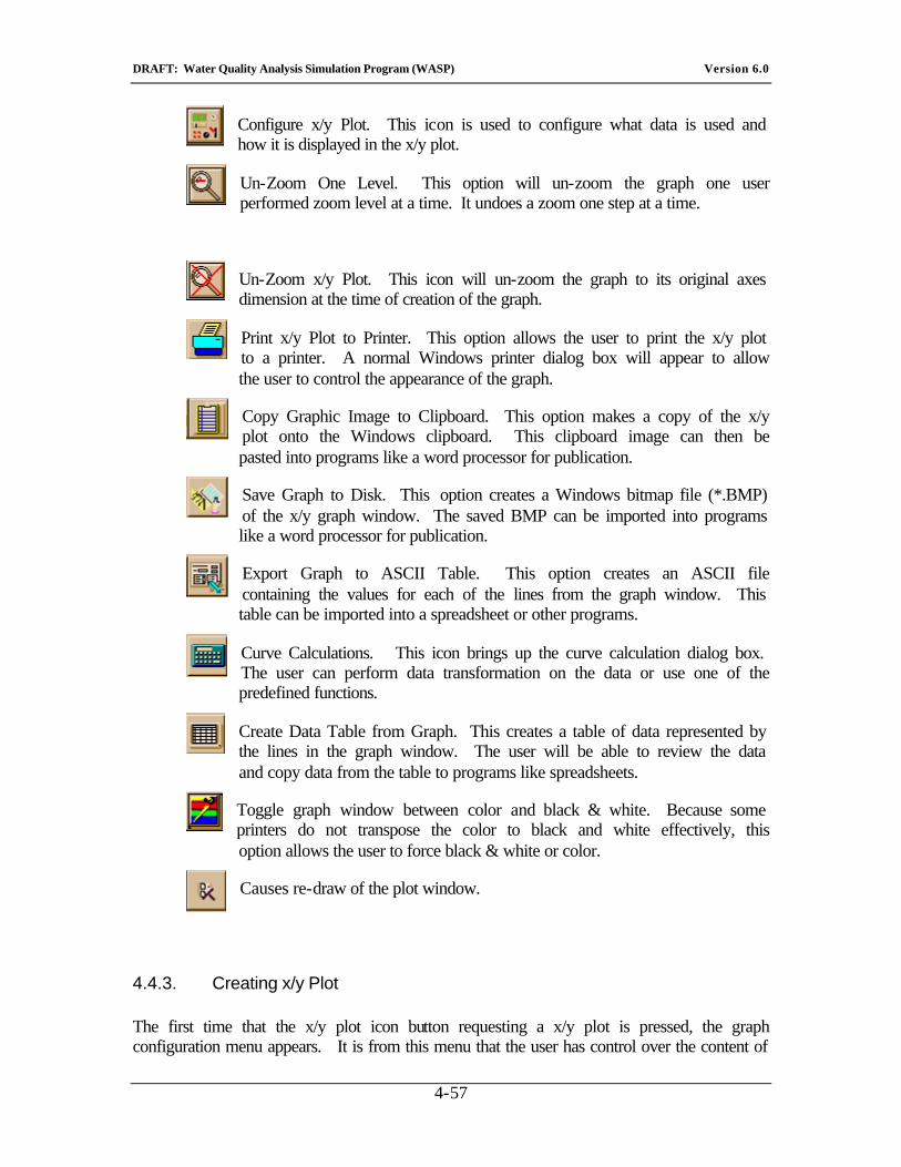
DRAFT: Water Quality Analysis Simulation Program (WASP) Version 6.0
4-57
Configure x/y Plot. This icon is used to configure what data is used and how it is displayed in the x/y plot.
Un-Zoom One Level. This option will un-zoom the graph one user performed zoom level at a time. It undoes a zoom one step at a time.
Un-Zoom x/y Plot. This icon will un-zoom the graph to its original axes dimension at the time of creation of the graph.
Print x/y Plot to Printer. This option allows the user to print the x/y plot to a printer. A normal Windows printer dialog box will appear to allow the user to control the appearance of the graph.
Copy Graphic Image to Clipboard. This option makes a copy of the x/y plot onto the Windows clipboard. This clipboard image can then be pasted into programs like a word processor for publication.
Save Graph to Disk. This option creates a Windows bitmap file (*.BMP) of the x/y graph window. The saved BMP can be imported into programs like a word processor for publication.
Export Graph to ASCII Table. This option creates an ASCII file containing the values for each of the lines from the graph window. This table can be imported into a spreadsheet or other programs.
Curve Calculations. This icon brings up the curve calculation dialog box. The user can perform data transformation on the data or use one of the predefined functions.
Create Data Table from Graph. This creates a table of data represented by the lines in the graph window. The user will be able to review the data and copy data from the table to programs like spreadsheets.
Toggle graph window between color and black & white. Because some printers do not transpose the color to black and white effectively, this option allows the user to force black & white or color.
Causes re-draw of the plot window.
4.4.3. Creating x/y Plot
The first time that the x/y plot icon button requesting a x/y plot is pressed, the graph configuration menu appears. It is from this menu that the user has control over the content of
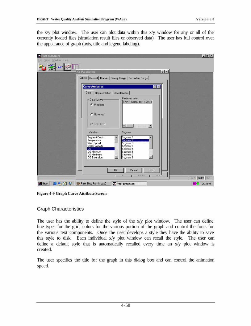
DRAFT: Water Quality Analysis Simulation Program (WASP) Version 6.0
4-58
the x/y plot window. The user can plot data within this x/y window for any or all of the currently loaded files (simulation result files or observed data). The user has full control over the appearance of graph (axis, title and legend labeling).
Figure 4-9 Graph Curve Attribute Screen
Graph Characteristics
The user has the ability to define the style of the x/y plot window. The user can define line types for the grid, colors for the various portion of the graph and control the fonts for the various text components. Once the user develops a style they have the ability to save this style to disk. Each individual x/y plot window can recall the style. The user can define a default style that is automatically recalled every time an x/y plot window is created.
The user specifies the title for the graph in this dialog box and can control the animation speed.
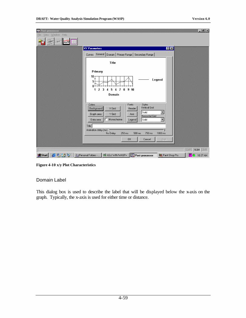
DRAFT: Water Quality Analysis Simulation Program (WASP) Version 6.0
4-59
Figure 4-10 x/y Plot Characteristics
Domain Label
This dialog box is used to describe the label that will be displayed below the x-axis on the graph. Typically, the x-axis is used for either time or distance.
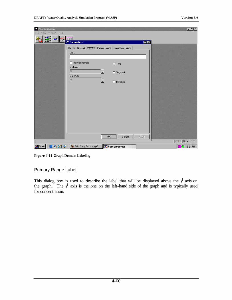
DRAFT: Water Quality Analysis Simulation Program (WASP) Version 6.0
4-60
Figure 4-11 Graph Domain Labeling
Primary Range Label
This dialog box is used to describe the label that will be displayed above the y1 axis on the graph. The y1 axis is the one on the left-hand side of the graph and is typically used for concentration.
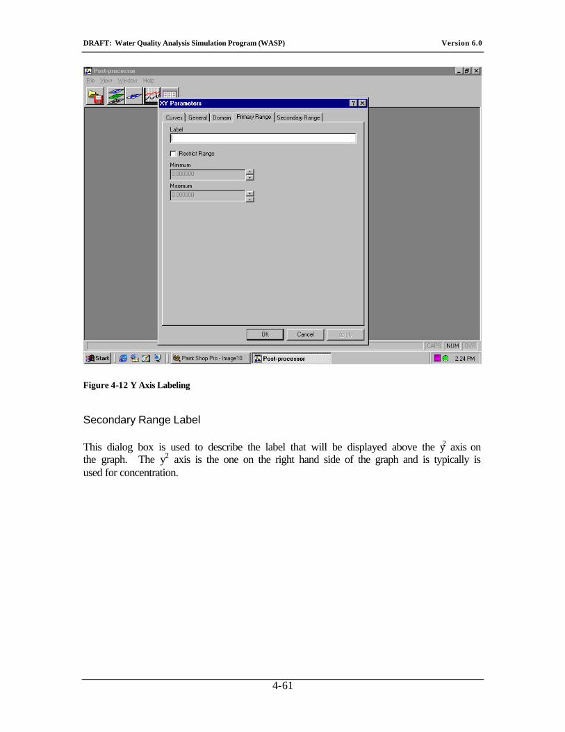
DRAFT: Water Quality Analysis Simulation Program (WASP) Version 6.0
4-61
Figure 4-12 Y Axis Labeling
Secondary Range Label
This dialog box is used to describe the label that will be displayed above the y2 axis on the graph. The y2 axis is the one on the right hand side of the graph and is typically is used for concentration.
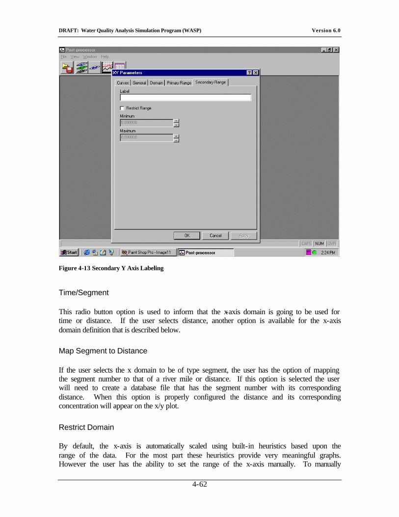
DRAFT: Water Quality Analysis Simulation Program (WASP) Version 6.0
4-62
Figure 4-13 Secondary Y Axis Labeling
Time/Segment
This radio button option is used to inform that the x-axis domain is going to be used for time or distance. If the user selects distance, another option is available for the x-axis domain definition that is described below.
Map Segment to Distance
If the user selects the x domain to be of type segment, the user has the option of mapping the segment number to that of a river mile or distance. If this option is selected the user will need to create a database file that has the segment number with its corresponding distance. When this option is properly configured the distance and its corresponding concentration will appear on the x/y plot.
Restrict Domain
By default, the x-axis is automatically scaled using built-in heuristics based upon the range of the data. For the most part these heuristics provide very meaningful graphs. However the user has the ability to set the range of the x-axis manually. To manually

DRAFT: Water Quality Analysis Simulation Program (WASP) Version 6.0
4-63
control the range of x-axis, the user should select the "restrict x-axis range" from the graph configuration window. Once this is selected, the user may enter values for the minimum and maximum values for the x-axis.
Note: There are more sophisticated methods for manipulating the range of the x-axis (see Zooming X-Axis).
Restrict y1/y2 Range
By default the y-axis is automatically scaled using built-in heuristics. For the most part these heuristics provide very meaningful graphs. However the user has the ability to set the scale of the y-axis manually. To enter a value for the y scale the user should select to restrict y-axis range from the graph configuration window. Once this is selected, the user may enter values for the minimum and maximum values for the y-axis being defined.
Note: The user can control the range for both the Y1 and Y2 axes.
Graph Title
This dialog box is used to describe the title that will be displayed at the top of the graph. The user is limited to 25 characters within the title line.
Animation Delay
The animation delay dialog box allows the user to define the delay when the user presses the animation button from the x/y toolbar.
Color/Black & White
This radio button selection works the same as if the user pressed the Color/Black & White icon from the toolbar. This will toggle the x/y plot between color and black & white.
Curve Definition
The curves dialog window indicates how many lines are currently defined for the given graph. To add a curve to the graph the user should press the Add Curve button. This will bring up the curve definition window. If the user wants to edit the attributes of a previously created curve the user should select the curve to be edited in the curve window
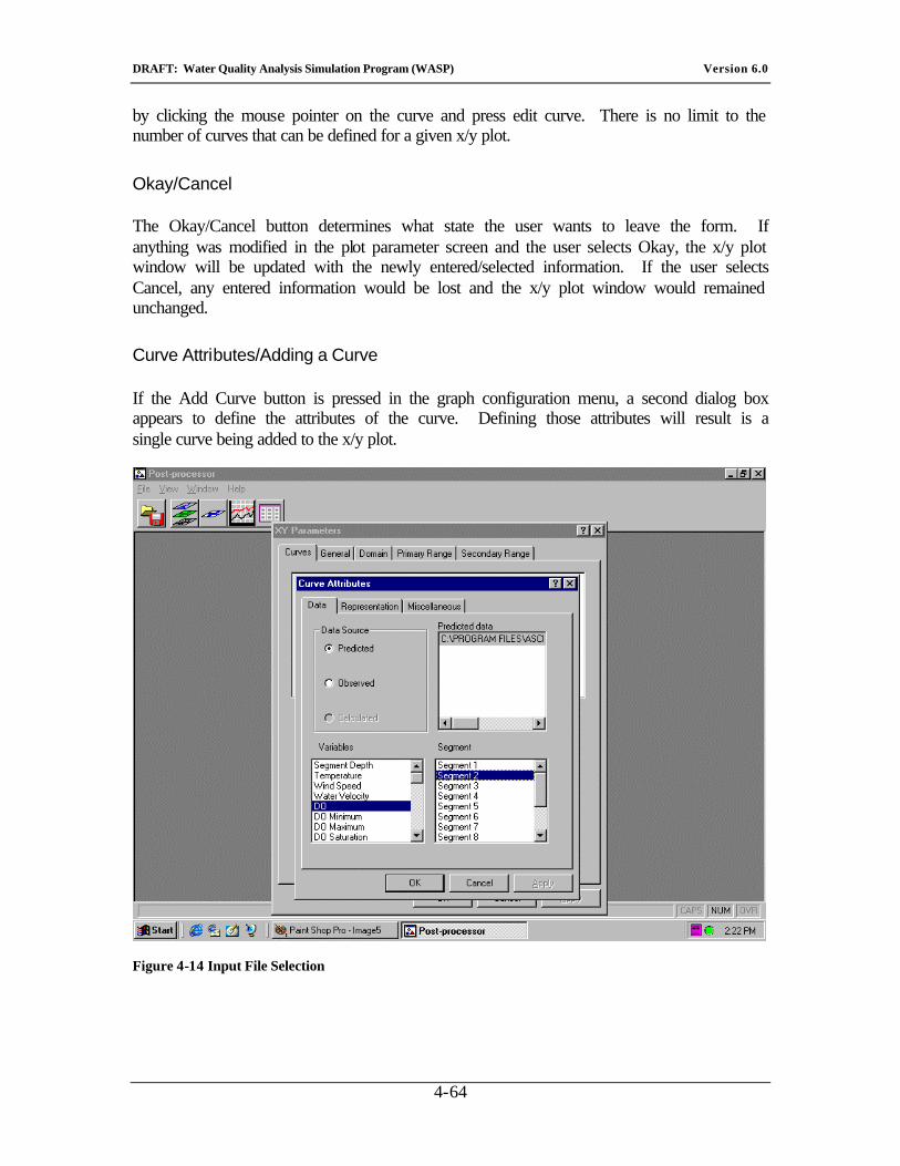
DRAFT: Water Quality Analysis Simulation Program (WASP) Version 6.0
4-64
by clicking the mouse pointer on the curve and press edit curve. There is no limit to the number of curves that can be defined for a given x/y plot.
Okay/Cancel
The Okay/Cancel button determines what state the user wants to leave the form. If anything was modified in the plot parameter screen and the user selects Okay, the x/y plot window will be updated with the newly entered/selected information. If the user selects Cancel, any entered information would be lost and the x/y plot window would remained unchanged.
Curve Attributes/Adding a Curve
If the Add Curve button is pressed in the graph configuration menu, a second dialog box appears to define the attributes of the curve. Defining those attributes will result is a single curve being added to the x/y plot.
Figure 4-14 Input File Selection
DRAFT: Water Quality Analysis Simulation Program (WASP) Version 6.0
4-65
Data Source
Data are obtained from several sources and are available for plotting within the x/y plot window. For the data to be available for a given plot window it must either be read into memory (read from disk: simulation result files or observed database) or created from a previous calculation.
The radio buttons located within the Data Source dialog window will be available for selection if the particular type is available for plotting. The model simulation results file and the observed data databases are loaded using the "Open File" dialog from the main menu. The calculated data sources are created from within the x/y plot window. A calculated data source created in one x/y plot window is available to other x/y plot windows as well.
Predicted
The predicted data type is assigned to the files that contain model simulation results.
Observed
The observed type is assigned to the observed data database. The observed data database must have a specific file format containing specifically named data fields.
Calculated
The user created the “calculated” field using built-in functions. One such function is the model partition function, where the user can calculate the difference between one curve and another. The results of this calculation are stored in a user defined Calculated data structure.
Selecting Data File
The selection of the data source radio buttons will determine the content of the data file dialog window. If a model simulation result file is loaded and the Predicted radio button is selected the filenames will appear in the Predicted Data window. The user selects the file to obtain plotting information from by pressing the left mouse button on the filename. The selected file will become highlighted. Once the file has been selected the user needs to select the variable and segment from which to retrieve information for plotting.
Selecting Variable
The variable list that is displayed in the variables dialog window is taken directly from the selected file. If it is a model simulation result file it will contain the output variables of either the hydrodynamic or water quality model.

DRAFT: Water Quality Analysis Simulation Program (WASP) Version 6.0
4-66
If the selected file is an "observed data" database, the variables are the names of stored constituents in the database. If the selected file was a calculated data structure, the name of the variable will be that assigned by the user when the calculated field was created.
To select and view the variables in list the user can use the scroll bar to move through the list. To select a variable to plot, the user should click the left mouse button on the desired variable to select. The selected variable will become highlighted.
Selecting Segment
The last item that has to be selected before an x/y plot can be created is what segment or computational element to plot. Once a Predicted Data file is selected, a list of the available segments to plot is displayed in the Segment dialog window. To select and view the segments in the list the user can use the scroll bar to move through the list. To select a segment to plot, the user should click the left mouse button on the desired segment. The selected variable will become highlighted. If the data source is an observed data database the segment is typically a station identification number.
Representation
The representation radio button dialog box allows the user to assign a specific characteristic for the defined curve. The user has the option of drawing a line, symbol, line & symbol or force solid for the defined curve.
Note: A different line style, color and symbol is automatically created for each line defined in a particular x/y plot window.
Second Y
The user may assign any number of the defined curves to the second y2 axis (scale located on the right hand side of graph). When a second y2 is requested, the curve assigned to that y2 axis will be scaled and plotted independently of any curve assigned to y1 axis.
Observed Data
Observed data can be added to any x/y plot window. Before observed data is available for plotting the observed data database must have been opened for use by the user. Observed data is opened using the open file dialog box. Once the observed data database has been opened the data will be available for plotting in the x/y plot window. To select observe data to plot, the user should press the Observed radio button. If there is more
DRAFT: Water Quality Analysis Simulation Program (WASP) Version 6.0
4-67
than one database file loaded, the user will be presented a choice of file in the predicted data window. The user should select the database file, select the variable from the variable window and then select the Station ID from the segment window.
Note: Observed data can be plotted exclusively if the user desires.
Legend Description
The user can control the information that is automatically placed in the x/y plot legend that is used to illustrate the contents of the graph. The user has four options for the legend:
1) Data Set – setting this radio button will cause the use of the dataset name selected in the Predicted Data dialog window for the legend of the defined line.
2) Variable -- setting this radio button will cause the use of the variable name selected in the Variable dialog window for the legend of the defined line.
3) Segment -- setting this radio button will cause the use of the segment name selected in the Segment dialog window for the legend of the defined line.
4) User-Defined -- setting this radio button will cause the use of the user-defined item to be placed in the User-Defined Dialog box.
Note: If the user does not want a legend, the user should select “user define” and not type anything into the user defined dialog box.
4.4.4. OK/Cancel
Once this information was been selected along with any other user definable parameters the user should press Okay to generate the graph. The observed data will be plotted on the x/y graph along with any predicted or user selected data. If they press cancel, all the information entered will be lost.
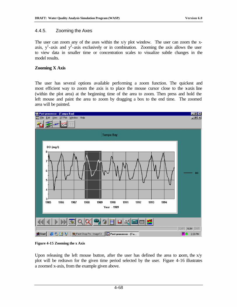
DRAFT: Water Quality Analysis Simulation Program (WASP) Version 6.0
4-68
4.4.5. Zooming the Axes
The user can zoom any of the axes within the x/y plot window. The user can zoom the x-axis, y1-axis and y2-axis exclusively or in combination. Zooming the axis allows the user to view data in smaller time or concentration scales to visualize subtle changes in the model results.
Zooming X Axis
The user has several options available performing a zoom function. The quickest and most efficient way to zoom the axis is to place the mouse cursor close to the x-axis line (within the plot area) at the beginning time of the area to zoom. Then press and hold the left mouse and paint the area to zoom by dragging a box to the end time. The zoomed area will be painted.
Figure 4-15 Zooming the x Axis
Upon releasing the left mouse button, after the user has defined the area to zoom, the x/y plot will be redrawn for the given time period selected by the user. Figure 4-16 illustrates a zoomed x-axis, from the example given above.
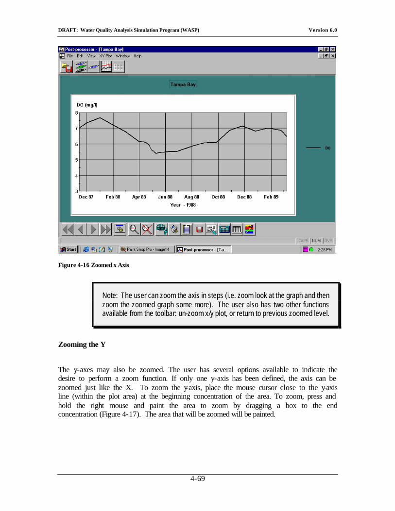
DRAFT: Water Quality Analysis Simulation Program (WASP) Version 6.0
4-69
Figure 4-16 Zoomed x Axis
Note: The user can zoom the axis in steps (i.e. zoom look at the graph and then zoom the zoomed graph some more). The user also has two other functions available from the toolbar: un-zoom x/y plot, or return to previous zoomed level.
Zooming the Y
The y-axes may also be zoomed. The user has several options available to indicate the desire to perform a zoom function. If only one y-axis has been defined, the axis can be zoomed just like the X. To zoom the y-axis, place the mouse cursor close to the y-axis line (within the plot area) at the beginning concentration of the area. To zoom, press and hold the right mouse and paint the area to zoom by dragging a box to the end concentration (Figure 4-17). The area that will be zoomed will be painted.
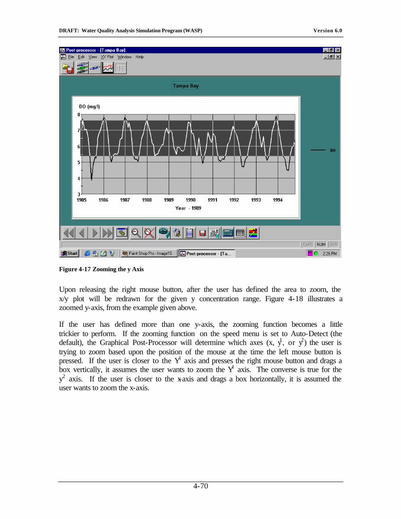
DRAFT: Water Quality Analysis Simulation Program (WASP) Version 6.0
4-70
Figure 4-17 Zooming the y Axis
Upon releasing the right mouse button, after the user has defined the area to zoom, the x/y plot will be redrawn for the given y concentration range. Figure 4-18 illustrates a zoomed y-axis, from the example given above.
If the user has defined more than one y-axis, the zooming function becomes a little trickier to perform. If the zooming function on the speed menu is set to Auto-Detect (the default), the Graphical Post-Processor will determine which axes (x, y1, or y2) the user is trying to zoom based upon the position of the mouse at the time the left mouse button is pressed. If the user is closer to the Y1 axis and presses the right mouse button and drags a box vertically, it assumes the user wants to zoom the Y1 axis. The converse is true for the y2 axis. If the user is closer to the x-axis and drags a box horizontally, it is assumed the user wants to zoom the x-axis.
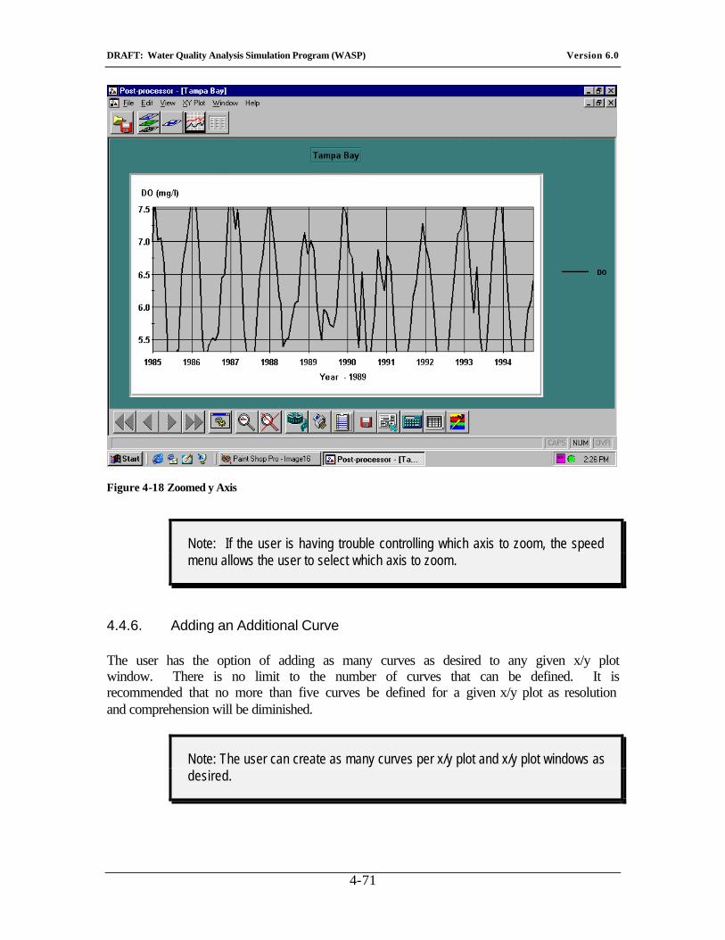
DRAFT: Water Quality Analysis Simulation Program (WASP) Version 6.0
4-71
Figure 4-18 Zoomed y Axis
Note: If the user is having trouble controlling which axis to zoom, the speed menu allows the user to select which axis to zoom.
4.4.6. Adding an Additional Curve
The user has the option of adding as many curves as desired to any given x/y plot window. There is no limit to the number of curves that can be defined. It is recommended that no more than five curves be defined for a given x/y plot as resolution and comprehension will be diminished.
Note: The user can create as many curves per x/y plot and x/y plot windows as desired.
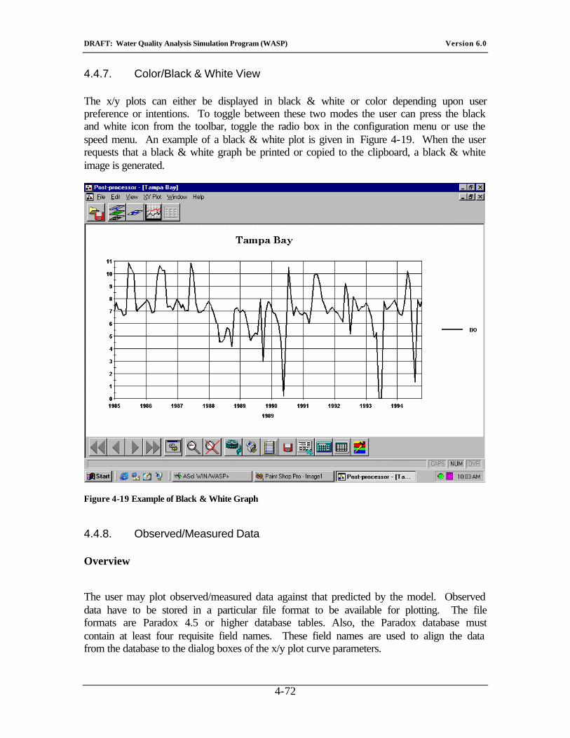
DRAFT: Water Quality Analysis Simulation Program (WASP) Version 6.0
4-72
4.4.7. Color/Black & White View
The x/y plots can either be displayed in black & white or color depending upon user preference or intentions. To toggle between these two modes the user can press the black and white icon from the toolbar, toggle the radio box in the configuration menu or use the speed menu. An example of a black & white plot is given in Figure 4-19. When the user requests that a black & white graph be printed or copied to the clipboard, a black & white image is generated.
Figure 4-19 Example of Black & White Graph
4.4.8. Observed/Measured Data
Overview
The user may plot observed/measured data against that predicted by the model. Observed data have to be stored in a particular file format to be available for plotting. The file formats are Paradox 4.5 or higher database tables. Also, the Paradox database must contain at least four requisite field names. These field names are used to align the data from the database to the dialog boxes of the x/y plot curve parameters.
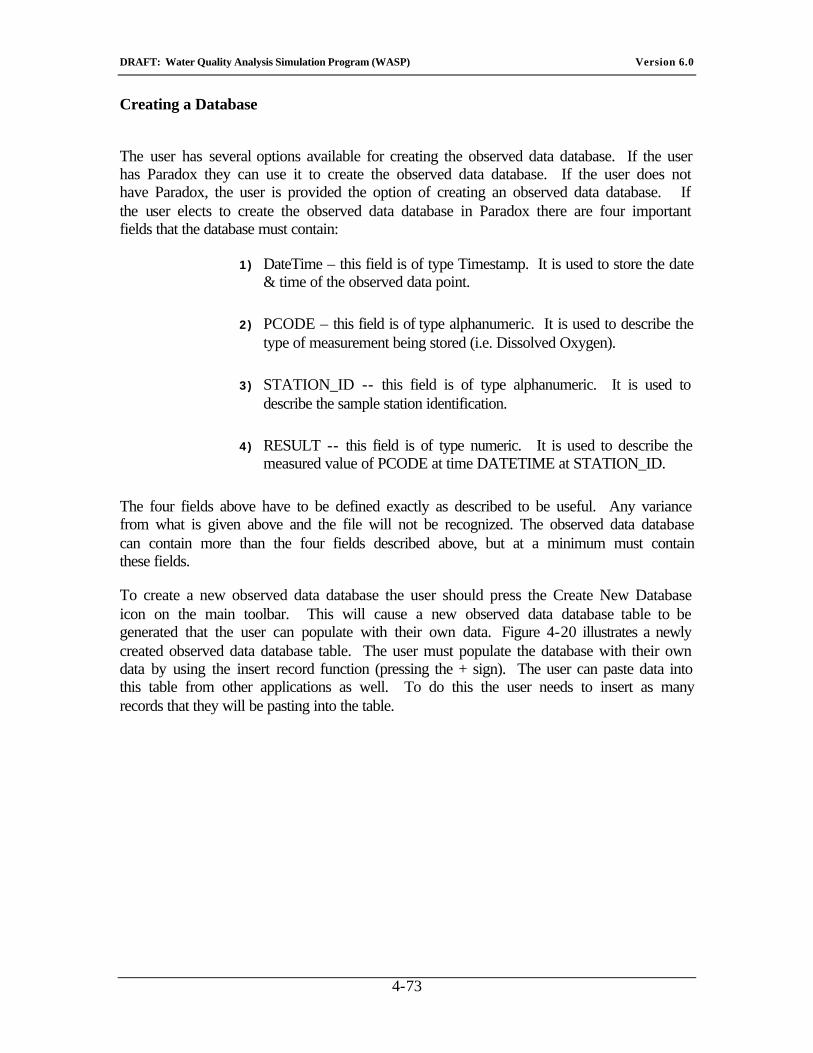
DRAFT: Water Quality Analysis Simulation Program (WASP) Version 6.0
4-73
Creating a Database
The user has several options available for creating the observed data database. If the user has Paradox they can use it to create the observed data database. If the user does not have Paradox, the user is provided the option of creating an observed data database. If the user elects to create the observed data database in Paradox there are four important fields that the database must contain:
1) DateTime – this field is of type Timestamp. It is used to store the date & time of the observed data point.
2) PCODE – this field is of type alphanumeric. It is used to describe the type of measurement being stored (i.e. Dissolved Oxygen).
3) STATION_ID -- this field is of type alphanumeric. It is used to describe the sample station identification.
4) RESULT -- this field is of type numeric. It is used to describe the measured value of PCODE at time DATETIME at STATION_ID.
The four fields above have to be defined exactly as described to be useful. Any variance from what is given above and the file will not be recognized. The observed data database can contain more than the four fields described above, but at a minimum must contain these fields.
To create a new observed data database the user should press the Create New Database icon on the main toolbar. This will cause a new observed data database table to be generated that the user can populate with their own data. Figure 4-20 illustrates a newly created observed data database table. The user must populate the database with their own data by using the insert record function (pressing the + sign). The user can paste data into this table from other applications as well. To do this the user needs to insert as many records that they will be pasting into the table.
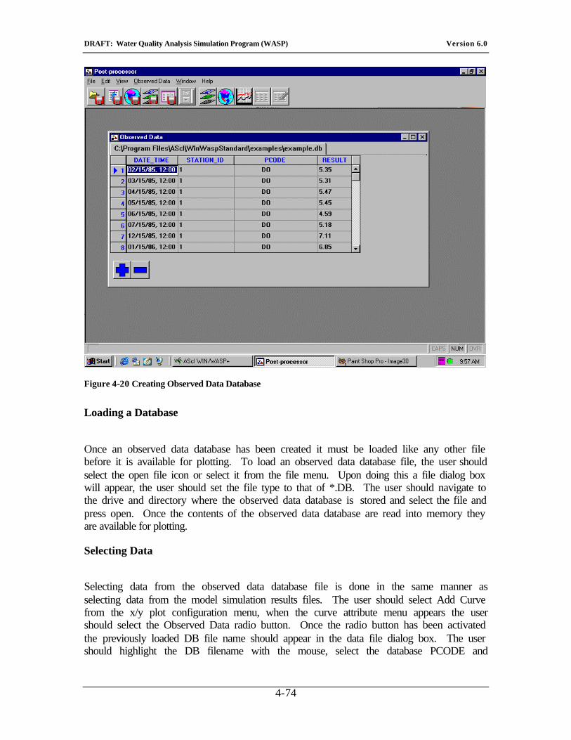
DRAFT: Water Quality Analysis Simulation Program (WASP) Version 6.0
4-74
Figure 4-20 Creating Observed Data Database
Loading a Database
Once an observed data database has been created it must be loaded like any other file before it is available for plotting. To load an observed data database file, the user should select the open file icon or select it from the file menu. Upon doing this a file dialog box will appear, the user should set the file type to that of *.DB. The user should navigate to the drive and directory where the observed data database is stored and select the file and press open. Once the contents of the observed data database are read into memory they are available for plotting.
Selecting Data
Selecting data from the observed data database file is done in the same manner as selecting data from the model simulation results files. The user should select Add Curve from the x/y plot configuration menu, when the curve attribute menu appears the user should select the Observed Data radio button. Once the radio button has been activated the previously loaded DB file name should appear in the data file dialog box. The user should highlight the DB filename with the mouse, select the database PCODE and
DRAFT: Water Quality Analysis Simulation Program (WASP) Version 6.0
4-75
Station_ID to plot. Once these items have been selected the user should press the Okay button and the graph will be re-drawn with observed data included.
Note: The user has the same control over the observed data’s appearance as the simulation results.
4.4.9. Printing Results
The user has the option of printing the currently active x/y plot to any installed Windows printer device (this could be a laser printer, color printer, fax, or even e-mail). The user has the option of either printing the x/y plots in full color or changing them to black and white before printing. Depending upon the printer and the users Window’s 95 setup, the printer may automatically convert the colors to gray scale before printing. This may or may not be advantageous, if the graphs appear “muddy” the user should convert the graphs to black and white before printing to a printer, saving to a file or copying to a clipboard.
To change a plot to black and white the user should either select the Black and White radio button from the configuration menu or press the Black & White/Color toggle icon from the toolbar.
To print the currently active x/y plot the user should press the print icon from the toolbar. A standard windows print dialog box will appear. The user can select the appropriate output device to print the figure.
To File
The user has the option of saving a bitmap file of the currently active x/y plot to a file. This is useful for saving simulation results for comparison or inclusion into a presentation or publication.
To save the currently active x/y plot to a file as a bitmap, the user should press the save graph to bitmap icon from the toolbar. The user will be given a standard windows file dialog box that allows the user to designate the drive, directory and filename.
To Clipboard
The user also has the ability to copy a graphic image of the currently active x/y plot to the Windows clipboard. Once an image is copied to the Windows clipboard it can be pasted into virtually any Windows program that has graphics support.

DRAFT: Water Quality Analysis Simulation Program (WASP) Version 6.0
4-76
To copy the graphics image to the clipboard the user should press the copy to clipboard icon from the toolbar. Once the image has been copied it is available for pasting.
4.4.10. Creating Tabled Data
Internal data structures are utilized to store the actual numbers that are used to generate the x/y plots. A method is provided for the user to create a table of the data that is represented in the current x/y plot. Pressing the data table icon on the x/y plot toolbar creates this table. This will cause the creation of a table of data as illustrated in Figure 4-21. The data in this table is “read-only”. This basically means the user can access the data by marking columns and rows of data and copying it to the Windows clipboard so that it can be pasted into another application (i.e. spreadsheet).
Figure 4-21 Example of Tabular Data from Graph
The user has no ability to modify the data and have the results appear in the x/y plot.
Exporting Data
The user may export the data that is used to generate the active x/y plot to an external file to 1) comma delimited ASCII files and 2) Paradox database files.
DRAFT: Water Quality Analysis Simulation Program (WASP) Version 6.0
4-77
The comma delimited ASCII file type writes the data from the graph in column format, each curve will consist of two columns (x & y values). The data is separated by commas and can be directly imported into most spreadsheet programs.
The Paradox file format creates a Paradox compatible database file of all the data in the x/y plot. This database table that is created can be read directly by Paradox or the Deliberator program (a component of WASP). Each x/y pair from the graph is given it’s own record in the database.
To initiate the export data option the user should press the export data icon on the x/y plot toolbar. This will bring up a file dialog box that allows the user to define the path and filename to save the exported data.
To select the file type in which to save the data the user should use the drop down list from the Save As type in the dialog box. Chose the appropriate type and give the file a name and press save.
4.4.11. Curve Calculations
A wide range of calculations can be performed on defined curves on the x/y plot. The curve calculation screen is entered by pressing the curve calculate button on the x/y plot toolbar. Curve calculations can only be performed on defined curves within the x/y plot window. The are several types of curve calculations that can be performed:
1) User Defined – functions that the user can derive to make calculation
2) Moving Average – user specifies the time interval for the moving average and generates a new curve depicting the results.
3) Frequency Distribution – the user specifies the number of concentration intervals to be used in the frequency distribution and calculation of the new curves.
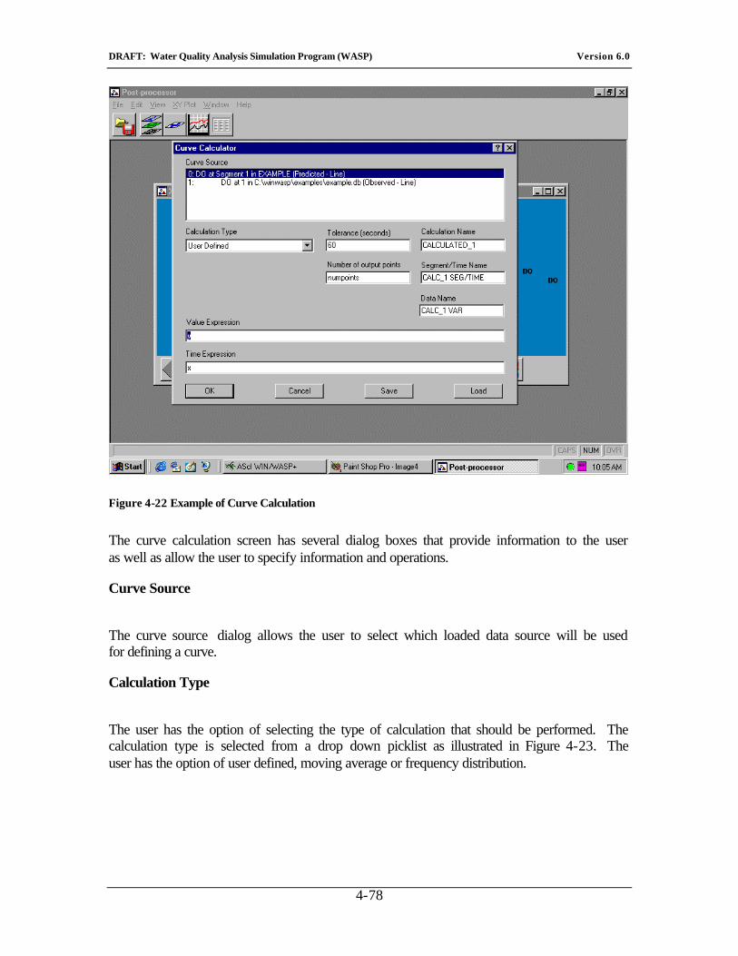
DRAFT: Water Quality Analysis Simulation Program (WASP) Version 6.0
4-78
Figure 4-22 Example of Curve Calculation
The curve calculation screen has several dialog boxes that provide information to the user as well as allow the user to specify information and operations.
Curve Source
The curve source dialog allows the user to select which loaded data source will be used for defining a curve.
Calculation Type
The user has the option of selecting the type of calculation that should be performed. The calculation type is selected from a drop down picklist as illustrated in Figure 4-23. The user has the option of user defined, moving average or frequency distribution.
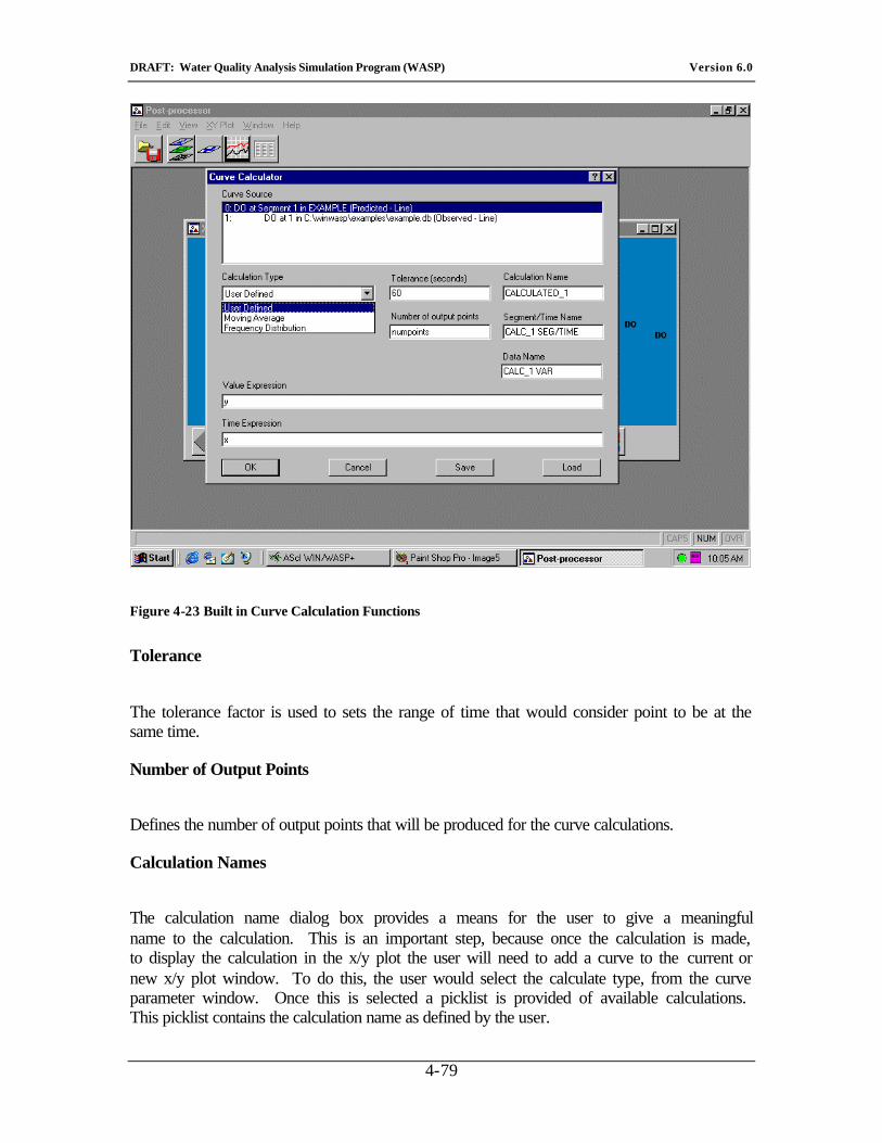
DRAFT: Water Quality Analysis Simulation Program (WASP) Version 6.0
4-79
Figure 4-23 Built in Curve Calculation Functions
Tolerance
The tolerance factor is used to sets the range of time that would consider point to be at the same time.
Number of Output Points
Defines the number of output points that will be produced for the curve calculations.
Calculation Names
The calculation name dialog box provides a means for the user to give a meaningful name to the calculation. This is an important step, because once the calculation is made, to display the calculation in the x/y plot the user will need to add a curve to the current or new x/y plot window. To do this, the user would select the calculate type, from the curve parameter window. Once this is selected a picklist is provided of available calculations. This picklist contains the calculation name as defined by the user.
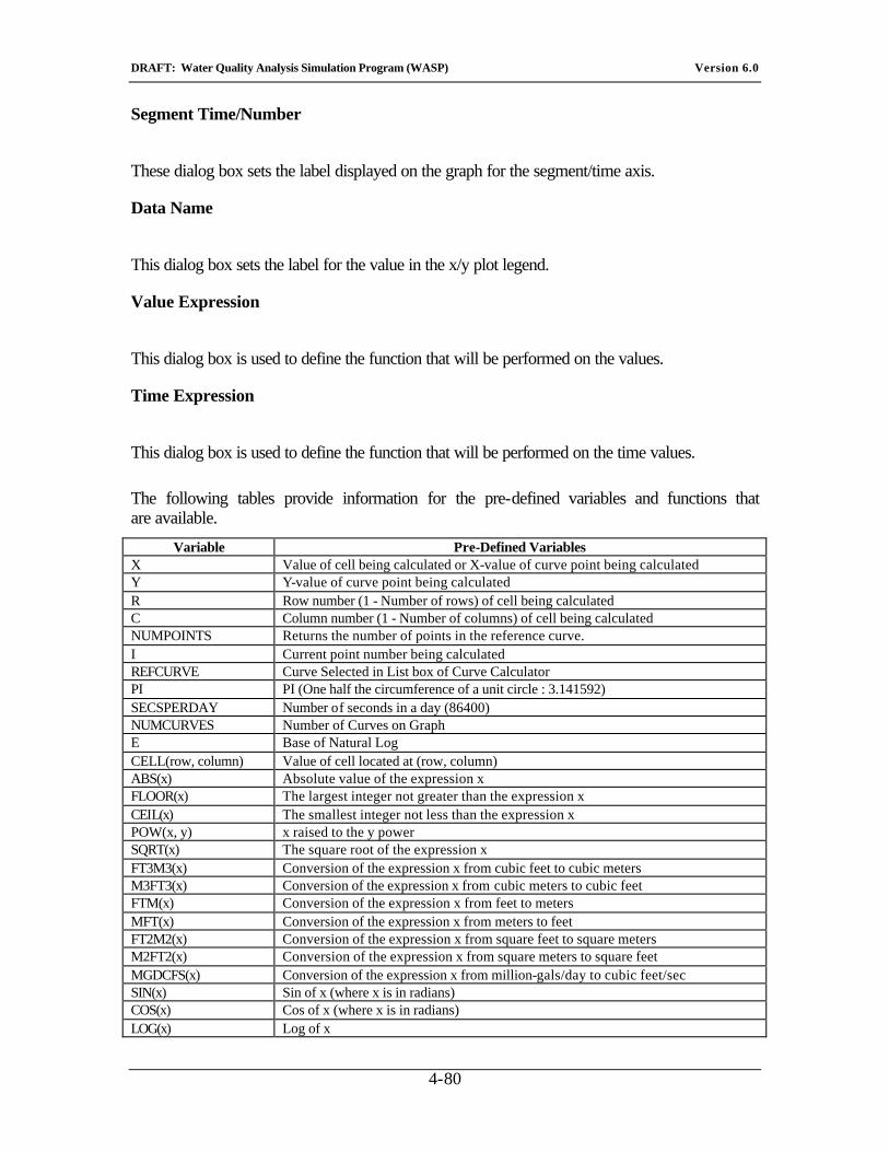
DRAFT: Water Quality Analysis Simulation Program (WASP) Version 6.0
4-80
Segment Time/Number
These dialog box sets the label displayed on the graph for the segment/time axis.
Data Name
This dialog box sets the label for the value in the x/y plot legend.
Value Expression
This dialog box is used to define the function that will be performed on the values.
Time Expression
This dialog box is used to define the function that will be performed on the time values.
The following tables provide information for the pre-defined variables and functions that are available.
Variable Pre-Defined Variables X Value of cell being calculated or X-value of curve point being calculated Y Y-value of curve point being calculated R Row number (1 - Number of rows) of cell being calculated C Column number (1 - Number of columns) of cell being calculated NUMPOINTS Returns the number of points in the reference curve. I Current point number being calculated REFCURVE Curve Selected in List box of Curve Calculator PI PI (One half the circumference of a unit circle : 3.141592) SECSPERDAY Number of seconds in a day (86400) NUMCURVES Number of Curves on Graph E Base of Natural Log CELL(row, column) Value of cell located at (row, column) ABS(x) Absolute value of the expression x FLOOR(x) The largest integer not greater than the expression x CEIL(x) The smallest integer not less than the expression x POW(x, y) x raised to the y power SQRT(x) The square root of the expression x FT3M3(x) Conversion of the expression x from cubic feet to cubic meters M3FT3(x) Conversion of the expression x from cubic meters to cubic feet FTM(x) Conversion of the expression x from feet to meters MFT(x) Conversion of the expression x from meters to feet FT2M2(x) Conversion of the expression x from square feet to square meters M2FT2(x) Conversion of the expression x from square meters to square feet MGDCFS(x) Conversion of the expression x from million-gals/day to cubic feet/sec SIN(x) Sin of x (where x is in radians) COS(x) Cos of x (where x is in radians) LOG(x) Log of x
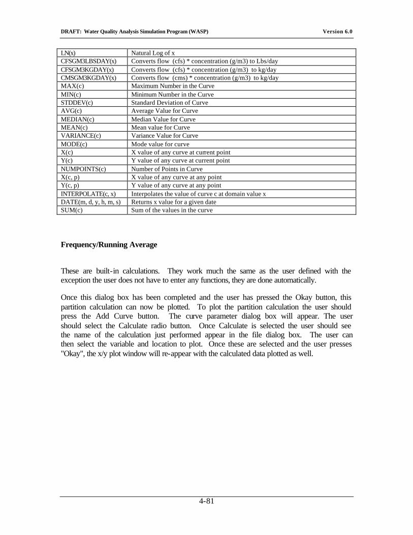
DRAFT: Water Quality Analysis Simulation Program (WASP) Version 6.0
4-81
LN(x) Natural Log of x CFSGM3LBSDAY(x) Converts flow (cfs) * concentration (g/m3) to Lbs/day CFSGM3KGDAY(x) Converts flow (cfs) * concentration (g/m3) to kg/day CMSGM3KGDAY(x) Converts flow (cms) * concentration (g/m3) to kg/day MAX(c) Maximum Number in the Curve MIN(c) Minimum Number in the Curve STDDEV(c) Standard Deviation of Curve AVG(c) Average Value for Curve MEDIAN(c) Median Value for Curve MEAN(c) Mean value for Curve VARIANCE(c) Variance Value for Curve MODE(c) Mode value for curve X(c) X value of any curve at current point Y(c) Y value of any curve at current point NUMPOINTS(c) Number of Points in Curve X(c, p) X value of any curve at any point Y(c, p) Y value of any curve at any point INTERPOLATE(c, x) Interpolates the value of curve c at domain value x DATE(m, d, y, h, m, s) Returns x value for a given date SUM(c) Sum of the values in the curve
Frequency/Running Average
These are built-in calculations. They work much the same as the user defined with the exception the user does not have to enter any functions, they are done automatically.
Once this dialog box has been completed and the user has pressed the Okay button, this partition calculation can now be plotted. To plot the partition calculation the user should press the Add Curve button. The curve parameter dialog box will appear. The user should select the Calculate radio button. Once Calculate is selected the user should see the name of the calculation just performed appear in the file dialog box. The user can then select the variable and location to plot. Once these are selected and the user presses "Okay", the x/y plot window will re-appear with the calculated data plotted as well.
DRAFT: Water Quality Analysis Simulation Program (WASP) Version 6.0
5-1
5. The Basic Water Quality Model
WASP6 is a dynamic compartment model that can be used to analyze a variety of water quality problems in such diverse water bodies as ponds, streams, lakes, reservoirs, rivers, estuaries, and coastal waters. This section presents an overview of the basic water quality model. Subsequent chapters detail the transport and transformation processes in WASP6 for various water quality constituents.
The equations solved by WASP6 are based on the key principle of the conservation of mass. This principle requires that the mass of each water quality constituent being investigated must be accounted for in one way or another. WASP6 traces each water quality constituent from the point of spatial and temporal input to its final point of export, conserving mass in space and time. To perform these mass balance computations, the user must supply WASP6 with input data defining seven important characteristics:
• simulation and output control • model segmentation • advective and dispersive transport • boundary concentrations • point and diffuse source waste loads • kinetic parameters, constants, and time functions • initial concentrations
These input data, together with the general WASP6 mass balance equations and the specific chemical kinetics equations, uniquely define a special set of water quality equations. These are numerically integrated by WASP6 as the simulation proceeds in time. At user-specified print intervals, WASP6 saves the values of all display variables for subsequent retrieval by the post-processor program. These programs allow the user to interactively produce graphs and tables of variables of all display variables.
5.1. General Mass Balance Equation
A mass balance equation for dissolved constituents in a body of water must account for all the material entering and leaving through direct and diffuse loading; advective and dispersive transport; and physical, chemical, and biological transformation. Consider the coordinate system shown in Equation 5-1, where the x- and y-coordinates are in the horizontal plane, and the z-coordinate is in the vertical plane.
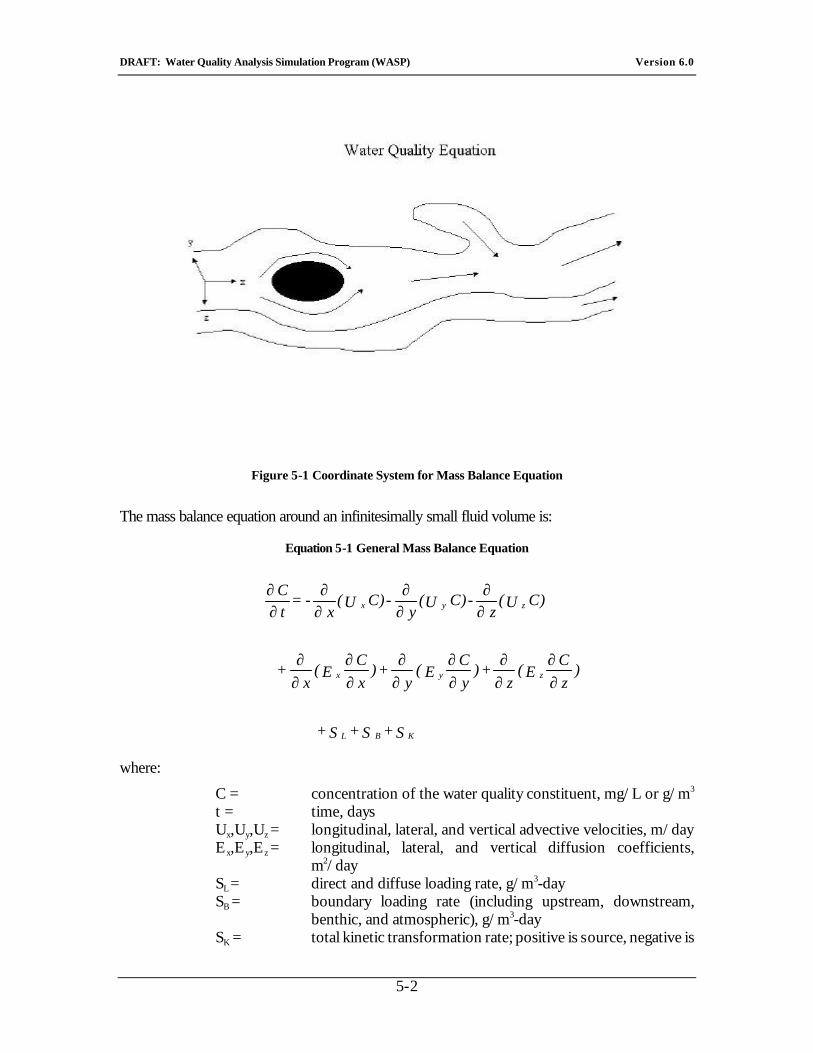
DRAFT: Water Quality Analysis Simulation Program (WASP) Version 6.0
5-2
Figure 5-1 Coordinate System for Mass Balance Equation
The mass balance equation around an infinitesimally small fluid volume is:
Equation 5-1 General Mass Balance Equation
S + S + S +
)z C
E( z
+ )y C
E( y
+ )x C
E( x
+
C) U(z
- C) U(y
- C) U( x
- = t C
K B L
z y x
z y x
∂∂
∂∂
∂∂
∂∂
∂∂
∂∂
∂∂
∂∂
∂∂
∂∂
where:
C = concentration of the water quality constituent, mg/L or g/m3 t = time, days Ux,Uy,Uz = longitudinal, lateral, and vertical advective velocities, m/day Ex,Ey,Ez = longitudinal, lateral, and vertical diffusion coefficients,
m2/day SL = direct and diffuse loading rate, g/m3-day SB = boundary loading rate (including upstream, downstream,
benthic, and atmospheric), g/m3-day SK = total kinetic transformation rate; positive is source, negative is
DRAFT: Water Quality Analysis Simulation Program (WASP) Version 6.0
5-3
sink, g/m3-day
By expanding the infinitesimally small control volumes into larger adjoining "segments," and by specifying proper transport, loading, and transformation parameters, WASP implements a finite-difference form of Equation 5-1. For brevity and clarity, however, the derivation of the finite-difference form of the mass balance equation will be for a one-dimensional reach. Assuming vertical and lateral homogeneity, we can integrate over y and z to obtain Equation 5-2
Equation 5-2 WASP Implementation of the Finite Difference Form of Mass Balance Equation
S A + )S + S( A + x C
A E + C A U - x
= C) (A t
K B L x x
∂∂
∂∂
∂∂
where:
A = cross-sectional area, m2
This equation represents the three major classes of water quality processes -- transport (term 1), loading (term 2), and transformation (term 3). The finite-difference form is derived in Appendix E. The model network and the major processes are discussed in the following sections.
5.2. The Model Network
The model network is a set of expanded control volumes, or “segments,” that together represents the physical configuration of the water body. As Figure 5-2 illustrates, the network may subdivide the water body laterally and vertically as well as longitudinally. Benthic segments can be included along with water column segments. If the water quality model is being linked to the hydrodynamic model, then water column segments must correspond to the hydrodynamic junctions. Concentrations of water quality constituents are calculated within each segment. Transport rates of water quality constituents are calculated across the interface of adjoining segments.
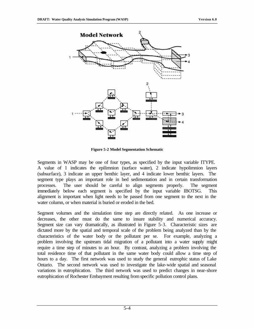
DRAFT: Water Quality Analysis Simulation Program (WASP) Version 6.0
5-4
Figure 5-2 Model Segmentation Schematic
Segments in WASP may be one of four types, as specified by the input variable ITYPE. A value of 1 indicates the epilimnion (surface water), 2 indicate hypolimnion layers (subsurface), 3 indicate an upper benthic layer, and 4 indicate lower benthic layers. The segment type plays an important role in bed sedimentation and in certain transformation processes. The user should be careful to align segments properly. The segment immediately below each segment is specified by the input variable IBOTSG. This alignment is important when light needs to be passed from one segment to the next in the water column, or when material is buried or eroded in the bed.
Segment volumes and the simulation time step are directly related. As one increase or decreases, the other must do the same to insure stability and numerical accuracy. Segment size can vary dramatically, as illustrated in Figure 5-3. Characteristic sizes are dictated more by the spatial and temporal scale of the problem being analyzed than by the characteristics of the water body or the pollutant per se. For example, analyzing a problem involving the upstream tidal migration of a pollutant into a water supply might require a time step of minutes to an hour. By contrast, analyzing a problem involving the total residence time of that pollutant in the same water body could allow a time step of hours to a day. The first network was used to study the general eutrophic status of Lake Ontario. The second network was used to investigate the lake-wide spatial and seasonal variations in eutrophication. The third network was used to predict changes in near-shore eutrophication of Rochester Embayment resulting from specific pollution control plans.
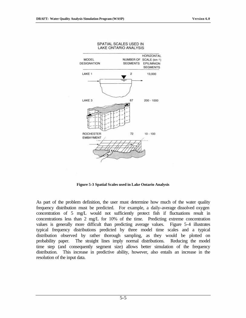
DRAFT: Water Quality Analysis Simulation Program (WASP) Version 6.0
5-5
Figure 5-3 Spatial Scales used in Lake Ontario Analysis
As part of the problem definition, the user must determine how much of the water quality frequency distribution must be predicted. For example, a daily-average dissolved oxygen concentration of 5 mg/L would not sufficiently protect fish if fluctuations result in concentrations less than 2 mg/L for 10% of the time. Predicting extreme concentration values is generally more difficult than predicting average values. Figure 5-4 illustrates typical frequency distributions predicted by three model time scales and a typical distribution observed by rather thorough sampling, as they would be plotted on probability paper. The straight lines imply normal distributions. Reducing the model time step (and consequently segment size) allows better simulation of the frequency distribution. This increase in predictive ability, however, also entails an increase in the resolution of the input data.
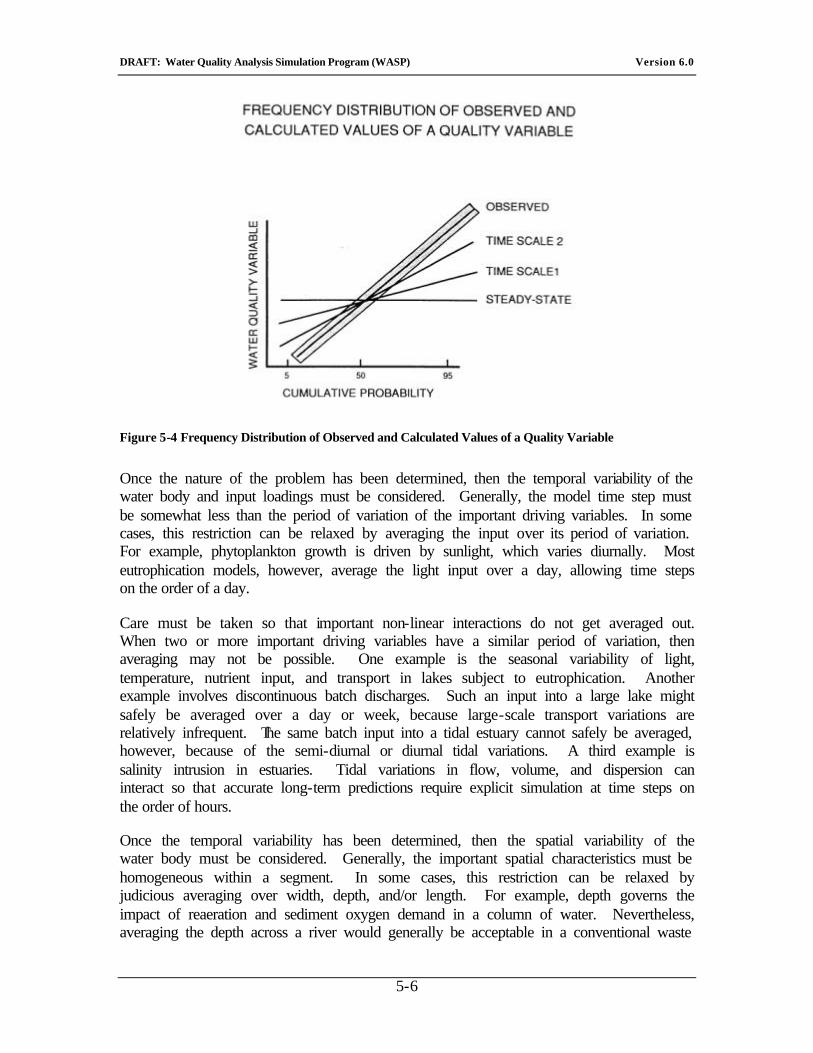
DRAFT: Water Quality Analysis Simulation Program (WASP) Version 6.0
5-6
Figure 5-4 Frequency Distribution of Observed and Calculated Values of a Quality Variable
Once the nature of the problem has been determined, then the temporal variability of the water body and input loadings must be considered. Generally, the model time step must be somewhat less than the period of variation of the important driving variables. In some cases, this restriction can be relaxed by averaging the input over its period of variation. For example, phytoplankton growth is driven by sunlight, which varies diurnally. Most eutrophication models, however, average the light input over a day, allowing time steps on the order of a day.
Care must be taken so that important non-linear interactions do not get averaged out. When two or more important driving variables have a similar period of variation, then averaging may not be possible. One example is the seasonal variability of light, temperature, nutrient input, and transport in lakes subject to eutrophication. Another example involves discontinuous batch discharges. Such an input into a large lake might safely be averaged over a day or week, because large-scale transport variations are relatively infrequent. The same batch input into a tidal estuary cannot safely be averaged, however, because of the semi-diurnal or diurnal tidal variations. A third example is salinity intrusion in estuaries. Tidal variations in flow, volume, and dispersion can interact so that accurate long-term predictions require explicit simulation at time steps on the order of hours.
Once the temporal variability has been determined, then the spatial variability of the water body must be considered. Generally, the important spatial characteristics must be homogeneous within a segment. In some cases, this restriction can be relaxed by judicious averaging over width, depth, and/or length. For example, depth governs the impact of reaeration and sediment oxygen demand in a column of water. Nevertheless, averaging the depth across a river would generally be acceptable in a conventional waste
DRAFT: Water Quality Analysis Simulation Program (WASP) Version 6.0
5-7
load allocation, whereas averaging the depth across a lake would not generally be acceptable. Other important spatial characteristics to consider (depending upon the problem being analyzed) include temperature, light penetration, velocity, pH, benthic characteristics or fluxes, and sediment concentrations.
The expected spatial variability of the water quality concentrations also affects the segment sizes. The user must determine how much averaging of the concentration gradients is acceptable. Because water quality conditions change rapidly near a loading point and stabilize downstream, studying the effects on a beach a quarter-mile downstream of a discharge requires smaller segments than studying the effects on a beach several miles away.
A final, general guideline may be helpful in obtaining accurate simulations: water column volumes should be roughly the same. If flows vary significantly downstream, then segment volumes should increase proportionately. The user should first choose the proper segment volume and time step in the critical reaches of the water body (Vc, Ätc), and then scale upstream and downstream segments accordingly:
Q/ Q V = V c i c i
Of course, actual volumes specified must be adjusted to best represent the actual spatial variability, as discussed above. This guideline will allow larger time steps and result in greater numerical accuracy over the entire model network, as explained in the section on "Simulation Parameters" in Chapter 2.
5.3. The Model Transport Scheme
Transport includes advection and dispersion of water quality constituents. Advection and dispersion in WASP are each divided into six distinct types, or "fields." The first transport field involves advective flow and dispersive mixing in the water column. Advective flow carries water quality constituents "downstream" with the water and accounts for instream dilution. Dispersion causes further mixing and dilution between regions of high concentrations and regions of low concentrations.
The second transport field specifies the movement of pore water in the sediment bed. Dissolved water quality constituents are carried through the bed by pore water flow and are exchanged between the bed and the water column by pore water diffusion.
The third, fourth, and fifth transport fields specify the transport of particulate pollutants by the settling, resuspension, and sedimentation of solids. Water quality constituents sorbed onto solid particles are transported between the water column and the sediment bed. The user can define the three solids fields as size fractions, such as sand, silt, and clay, or as inorganic, phytoplankton, and organic solids.
The sixth transport field represents evaporation or precipitation from or to surface water segments.

DRAFT: Water Quality Analysis Simulation Program (WASP) Version 6.0
5-8
Most transport data, such as flows or settling velocities, must be specified by the user in a WASP input dataset. For water column flow, however, the user may "link" WASP with a hydrodynamics model. If this option is specified, during the simulation WASP will read the contents of a hydrodynamic file for unsteady flows, volumes, depths, and velocities.
5.4. Application of the Model
The first step in applying the model is analyzing the problem to be solved. What questions are being asked? How can a simulation model be used to address these questions? A water quality model can do three basic tasks-- describe present water quality conditions, provide generic predictions, and provide site-specific predictions. The first, descriptive task is to extend in some way a limited site-specific database. Because monitoring is expensive, data seldom give the spatial and temporal resolution needed to fully characterize a water body. A simulation model can be used to interpolate between observed data, locating, for example, the dissolved oxygen sag point in a river or the maximum salinity intrusion in an estuary. Of course such a model can be used to guide future monitoring efforts. Descriptive models also can be used to infer the important processes controlling present water quality. This information can be used to guide not only monitoring efforts, but also model development efforts.
Providing generic predictions is a second type of modeling task. Site-specific data may not be needed if the goal is to predict the types of water bodies at risk from a new chemical. A crude set of data may be adequate to screen a list of chemicals for potential risk to a particular water body. Generic predictions may sufficiently address the management problem to be solved, or they may be a preliminary step in detailed site-specific analyses.
Providing site-specific predictions is the most stringent modeling task. Calibration to a good set of monitoring data is definitely needed to provide credible predictions. Because predictions often attempt to extrapolate beyond the present database, however, the model also must have sufficient process integrity. Examples of this type of application include waste load allocation to protect water quality standards and feasibility analysis for remedial actions, such as tertiary treatment, phosphate bans, or agricultural best-management practices.
Analysis of the problem should dictate the spatial and temporal scales for the modeling analysis. Division of the water body into appropriately sized segments was discussed in Section "Model Network." The user must try to extend the network upstream and downstream beyond the influence of the waste loads being studied. If this is not possible, the user should extend the network far enough so that errors in specifying future boundary concentrations do not propagate into the reaches being studied.
The user also should consider aligning the network so that sampling stations and points of interest (such as water withdrawals) fall near the center of a segment. Point source waste loads in streams and rivers with unidirectional flow should be located near the upper end of a segment. In estuaries and other water bodies with oscillating flow, waste loads are best centered within segments. If flows are to be input from DYNHYD, then a WASP

DRAFT: Water Quality Analysis Simulation Program (WASP) Version 6.0
5-9
segment must coincide with each hydrodynamic junction. Benthic segments, which are not present in the hydrodynamic network, may nevertheless be included in the WASP network. WASP segment numbering does not have to be the same as DYNHYD junction numbering. Segments stacked vertically do not have to be numbered consecutively from surface water segments down.
Once the network is set up, the model study will proceed through four general steps involving, in some manner, hydrodynamics, mass transport, water quality transformations, and environmental toxicology. The first step addresses the question of where the water goes. This can be answered by a combination of gaging, special studies, and hydrodynamic modeling. Flow data can be interpolated or extrapolated using the principle of continuity. Very simple flow routing models can be used; very complicated multi-dimensional hydrodynamic models can also be used with proper averaging over time and space. At present, the most compatible hydrodynamic model is DYNHYD.
The second step answers the question of where the material in the water is transported. This can be answered by a combination of tracer studies and model calibration. Dye and salinity are often used as tracers.
The third step answers the question of how the material in the water and sediment is transformed and what its fate is. This is the main focus of many studies. Answers depend on a combination of laboratory studies, field monitoring, parameter estimation, calibration, and testing. The net result is sometimes called model validation or verification, which are elusive concepts. The success of this step depends on the skill of the user, who must combine specialized knowledge with common sense and skepticism into a methodical process.
The final step answers the question of how this material is likely to affect anything of interest, such as people, fish, or the ecological balance. Often, predicted concentrations are simply compared with water quality criteria adopted to protect the general aquatic community. Care must be taken to insure that the temporal and spatial scales assumed in developing the criteria are compatible with those predicted by the model. Sometimes principles of physical chemistry or pharmacokinetics are used to predict chemical body burdens and resulting biological effects. The bioaccumulation model FGETS (Barber, et al., 1991) and the WASTOX food chain model (Connolly and Thomann, 1985) are good examples of this.
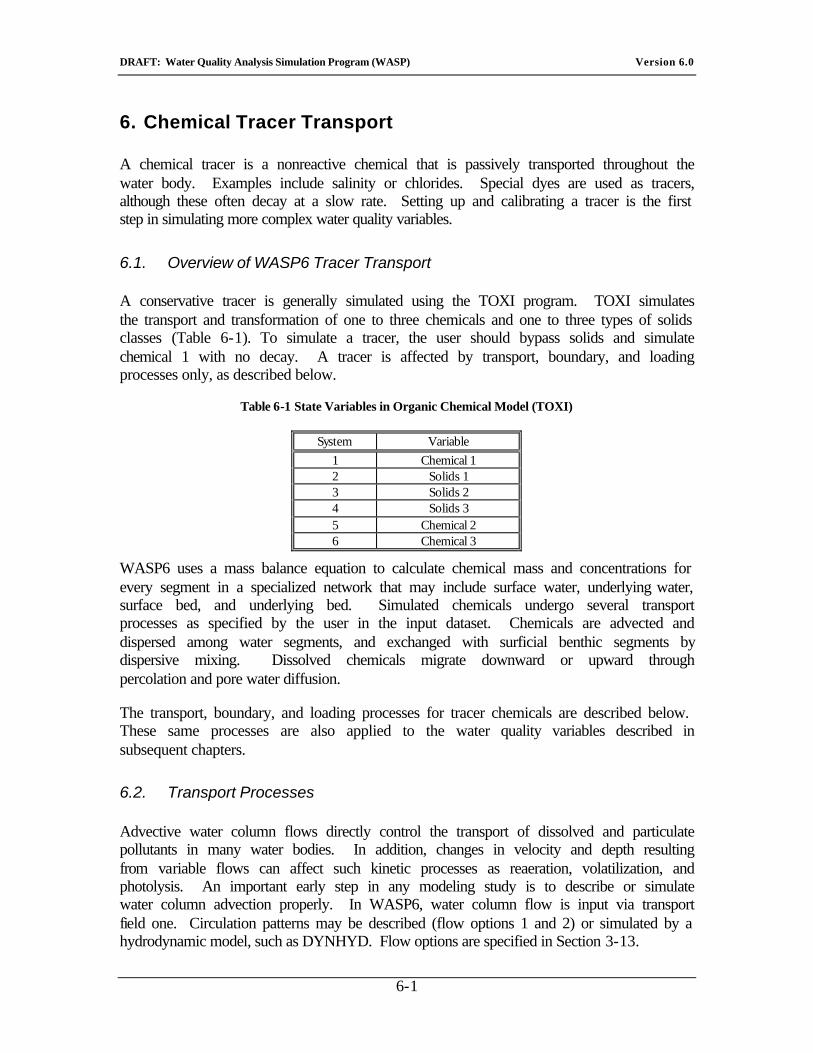
DRAFT: Water Quality Analysis Simulation Program (WASP) Version 6.0
6-1
6. Chemical Tracer Transport
A chemical tracer is a nonreactive chemical that is passively transported throughout the water body. Examples include salinity or chlorides. Special dyes are used as tracers, although these often decay at a slow rate. Setting up and calibrating a tracer is the first step in simulating more complex water quality variables.
6.1. Overview of WASP6 Tracer Transport
A conservative tracer is generally simulated using the TOXI program. TOXI simulates the transport and transformation of one to three chemicals and one to three types of solids classes (Table 6-1). To simulate a tracer, the user should bypass solids and simulate chemical 1 with no decay. A tracer is affected by transport, boundary, and loading processes only, as described below.
Table 6-1 State Variables in Organic Chemical Model (TOXI)
System Variable
1 Chemical 1 2 Solids 1 3 Solids 2 4 Solids 3 5 Chemical 2 6 Chemical 3
WASP6 uses a mass balance equation to calculate chemical mass and concentrations for every segment in a specialized network that may include surface water, underlying water, surface bed, and underlying bed. Simulated chemicals undergo several transport processes as specified by the user in the input dataset. Chemicals are advected and dispersed among water segments, and exchanged with surficial benthic segments by dispersive mixing. Dissolved chemicals migrate downward or upward through percolation and pore water diffusion.
The transport, boundary, and loading processes for tracer chemicals are described below. These same processes are also applied to the water quality variables described in subsequent chapters.
6.2. Transport Processes
Advective water column flows directly control the transport of dissolved and particulate pollutants in many water bodies. In addition, changes in velocity and depth resulting from variable flows can affect such kinetic processes as reaeration, volatilization, and photolysis. An important early step in any modeling study is to describe or simulate water column advection properly. In WASP6, water column flow is input via transport field one. Circulation patterns may be described (flow options 1 and 2) or simulated by a hydrodynamic model, such as DYNHYD. Flow options are specified in Section 3-13.
DRAFT: Water Quality Analysis Simulation Program (WASP) Version 6.0
6-2
For descriptive flows, WASP6 tracks each separate inflow specified by the user from its point of origin through the model network. For each inflow, the user must supply a continuity or unit flow response function and a time function. The time function describes the inflow as it varies in time. The continuity function describes the unit flow response as it varies throughout the network. The actual flow between segments that results from the inflow is the product of the time function and the continuity function.
If several inflow functions are specified, then the total flow between segments is the sum of the individual flow functions. Segment volumes are adjusted to maintain continuity. In this manner, the effect of several tributaries, density currents, and wind-induced gyres can be described.
In flow (Figure 3-6) Net Flow Option, WASP6 sums all the flows at a segment interface to determine the direction of net flow, and then moves mass in the ONE direction. In Gross Flow Option, WASP6 moves mass independently of net flow. For example, if opposite flows are specified at an interface, WASP6 will move mass in BOTH directions. This option allows the user to describe large dispersive circulation patterns.
6.2.1. Hydrodynamic Linkage
For unsteady flow in long networks, lag times may become significant, and hydrodynamic simulations may be necessary to obtain sufficient accuracy. Realistic simulations of unsteady transport can be accomplished by linking WASP6 to a compatible hydrodynamic simulation. This linkage is accomplished through an external file chosen by the user at simulation time. The hydrodynamic file contains segment volumes at the beginning of each time step, and average segment interfacial flows during each time step. WASP6 uses the interfacial flows to calculate mass transport, and the volumes to calculate constituent concentrations. Segment depths and velocities may also be contained in the hydrodynamic file for use in calculating reaeration and volatilization rates.
The first step in the hydrodynamic linkage is to develop a hydrodynamic calculational network that is compatible with the WASP6 network. The easiest linkage is with link-node hydrodynamic models that run on equivalent spatial networks. An example is given in Figure 6-1. Note that each WASP6 segment corresponds exactly to a hydrodynamic volume element, or node. Each WASP6 segment interface corresponds exactly to a hydrodynamic link, denoted in the figure with a connecting line.
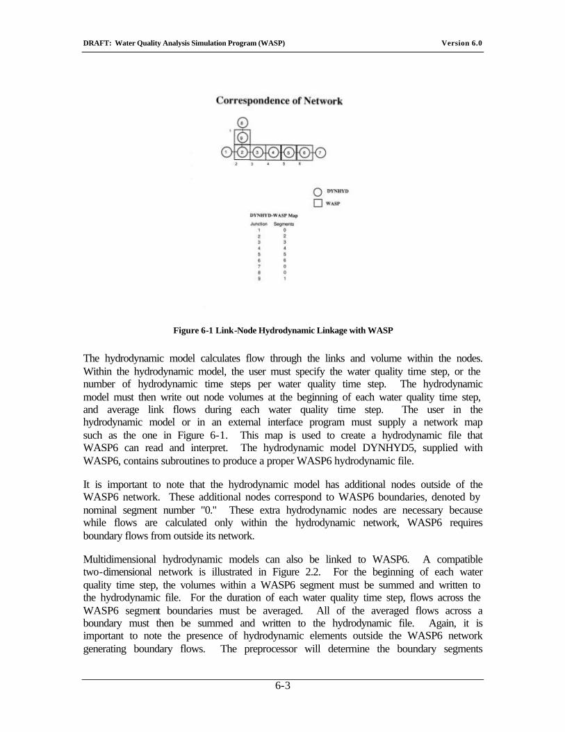
DRAFT: Water Quality Analysis Simulation Program (WASP) Version 6.0
6-3
Figure 6-1 Link-Node Hydrodynamic Linkage with WASP
The hydrodynamic model calculates flow through the links and volume within the nodes. Within the hydrodynamic model, the user must specify the water quality time step, or the number of hydrodynamic time steps per water quality time step. The hydrodynamic model must then write out node volumes at the beginning of each water quality time step, and average link flows during each water quality time step. The user in the hydrodynamic model or in an external interface program must supply a network map such as the one in Figure 6-1. This map is used to create a hydrodynamic file that WASP6 can read and interpret. The hydrodynamic model DYNHYD5, supplied with WASP6, contains subroutines to produce a proper WASP6 hydrodynamic file.
It is important to note that the hydrodynamic model has additional nodes outside of the WASP6 network. These additional nodes correspond to WASP6 boundaries, denoted by nominal segment number "0." These extra hydrodynamic nodes are necessary because while flows are calculated only within the hydrodynamic network, WASP6 requires boundary flows from outside its network.
Multidimensional hydrodynamic models can also be linked to WASP6. A compatible two-dimensional network is illustrated in Figure 2.2. For the beginning of each water quality time step, the volumes within a WASP6 segment must be summed and written to the hydrodynamic file. For the duration of each water quality time step, flows across the WASP6 segment boundaries must be averaged. All of the averaged flows across a boundary must then be summed and written to the hydrodynamic file. Again, it is important to note the presence of hydrodynamic elements outside the WASP6 network generating boundary flows. The preprocessor will determine the boundary segments
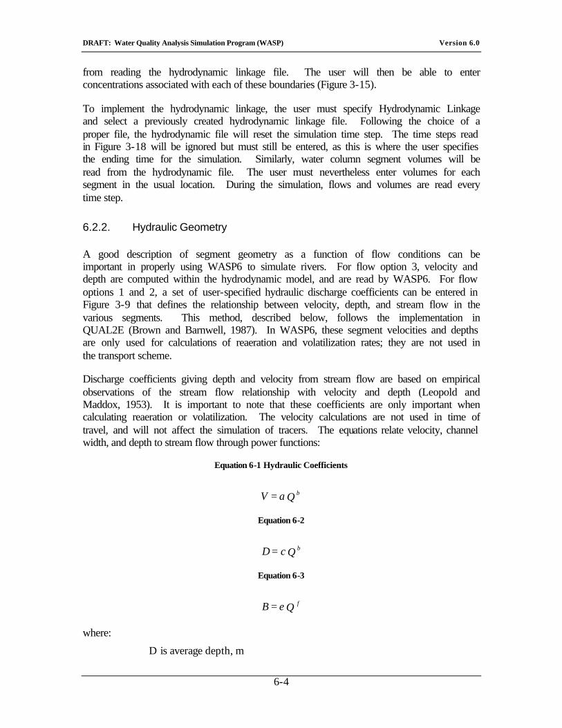
DRAFT: Water Quality Analysis Simulation Program (WASP) Version 6.0
6-4
from reading the hydrodynamic linkage file. The user will then be able to enter concentrations associated with each of these boundaries (Figure 3-15).
To implement the hydrodynamic linkage, the user must specify Hydrodynamic Linkage and select a previously created hydrodynamic linkage file. Following the choice of a proper file, the hydrodynamic file will reset the simulation time step. The time steps read in Figure 3-18 will be ignored but must still be entered, as this is where the user specifies the ending time for the simulation. Similarly, water column segment volumes will be read from the hydrodynamic file. The user must nevertheless enter volumes for each segment in the usual location. During the simulation, flows and volumes are read every time step.
6.2.2. Hydraulic Geometry
A good description of segment geometry as a function of flow conditions can be important in properly using WASP6 to simulate rivers. For flow option 3, velocity and depth are computed within the hydrodynamic model, and are read by WASP6. For flow options 1 and 2, a set of user-specified hydraulic discharge coefficients can be entered in Figure 3-9 that defines the relationship between velocity, depth, and stream flow in the various segments. This method, described below, follows the implementation in QUAL2E (Brown and Barnwell, 1987). In WASP6, these segment velocities and depths are only used for calculations of reaeration and volatilization rates; they are not used in the transport scheme.
Discharge coefficients giving depth and velocity from stream flow are based on empirical observations of the stream flow relationship with velocity and depth (Leopold and Maddox, 1953). It is important to note that these coefficients are only important when calculating reaeration or volatilization. The velocity calculations are not used in time of travel, and will not affect the simulation of tracers. The equations relate velocity, channel width, and depth to stream flow through power functions:
Equation 6-1 Hydraulic Coefficients
Q a = V b
Equation 6-2
Q c = D b
Equation 6-3
Q e = B f
where:
D is average depth, m
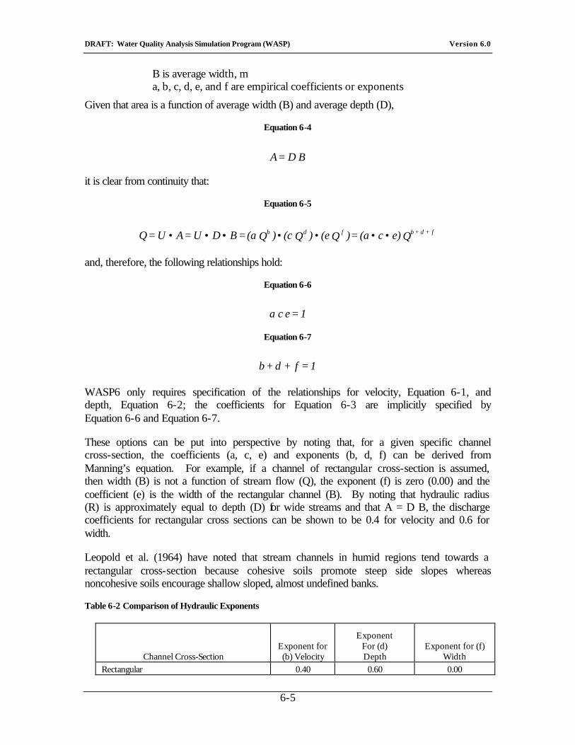
DRAFT: Water Quality Analysis Simulation Program (WASP) Version 6.0
6-5
B is average width, m a, b, c, d, e, and f are empirical coefficients or exponents
Given that area is a function of average width (B) and average depth (D),
Equation 6-4
B D = A
it is clear from continuity that:
Equation 6-5
Q e) c (a = )Q (e )Q (c )Q (a = B D U = A U = Q f + d + bfdb •••••••
and, therefore, the following relationships hold:
Equation 6-6
1 = e c a
Equation 6-7
1 = f + d + b
WASP6 only requires specification of the relationships for velocity, Equation 6-1, and depth, Equation 6-2; the coefficients for Equation 6-3 are implicitly specified by Equation 6-6 and Equation 6-7.
These options can be put into perspective by noting that, for a given specific channel cross-section, the coefficients (a, c, e) and exponents (b, d, f) can be derived from Manning’s equation. For example, if a channel of rectangular cross-section is assumed, then width (B) is not a function of stream flow (Q), the exponent (f) is zero (0.00) and the coefficient (e) is the width of the rectangular channel (B). By noting that hydraulic radius (R) is approximately equal to depth (D) for wide streams and that A = D B, the discharge coefficients for rectangular cross sections can be shown to be 0.4 for velocity and 0.6 for width.
Leopold et al. (1964) have noted that stream channels in humid regions tend towards a rectangular cross-section because cohesive soils promote steep side slopes whereas noncohesive soils encourage shallow sloped, almost undefined banks.
Table 6-2 Comparison of Hydraulic Exponents
Channel Cross-Section Exponent for (b) Velocity
Exponent For (d) Depth
Exponent for (f) Width
Rectangular 0.40 0.60 0.00
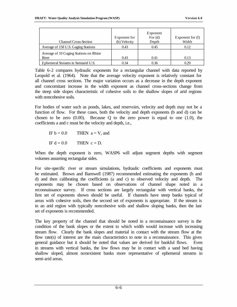
DRAFT: Water Quality Analysis Simulation Program (WASP) Version 6.0
6-6
Channel Cross-Section Exponent for (b) Velocity
Exponent For (d) Depth
Exponent for (f) Width
Average of 158 U.S. Gaging Stations 0.43 0.45 0.12
Average of 10 Gaging Stations on Rhine River 0.43 0.41 0.13 Ephemeral Streams in Semiarid U.S. 0.34 0.36 0.29
Table 6-2 compares hydraulic exponents for a rectangular channel with data reported by Leopold et al. (1964). Note that the average velocity exponent is relatively constant for all channel cross sections. The major variation occurs as a decrease in the depth exponent and concomitant increase in the width exponent as channel cross-sections change from the steep side slopes characteristic of cohesive soils to the shallow slopes of arid regions with noncohesive soils.
For bodies of water such as ponds, lakes, and reservoirs, velocity and depth may not be a function of flow. For these cases, both the velocity and depth exponents (b and d) can be chosen to be zero (0.00). Because Q to the zero power is equal to one (1.0), the coefficients a and c must be the velocity and depth, i.e.,
IF b = 0.0 THEN a = V, and
IF d = 0.0 THEN c = D.
When the depth exponent is zero, WASP6 will adjust segment depths with segment volumes assuming rectangular sides.
For site-specific river or stream simulations, hydraulic coefficients and exponents must be estimated. Brown and Barnwell (1987) recommended estimating the exponents (b and d) and then calibrating the coefficients (a and c) to observed velocity and depth. The exponents may be chosen based on observations of channel shape noted in a reconnaissance survey. If cross sections are largely rectangular with vertical banks, the first set of exponents shown should be useful. If channels have steep banks typical of areas with cohesive soils, then the second set of exponents is appropriate. If the stream is in an arid region with typically noncohesive soils and shallow sloping banks, then the last set of exponents is recommended.
The key property of the channel that should be noted in a reconnaissance survey is the condition of the bank slopes or the extent to which width would increase with increasing stream flow. Clearly the bank slopes and material in contact with the stream flow at the flow rate(s) of interest are the main characteristics to note in a reconnaissance. This gives general guidance but it should be noted that values are derived for bankful flows. Even in streams with vertical banks, the low flows may be in contact with a sand bed having shallow sloped, almost nonexistent banks more representative of ephemeral streams in semi-arid areas.

DRAFT: Water Quality Analysis Simulation Program (WASP) Version 6.0
6-7
6.2.3. Pore Water Advection
Pore water flows into or out of the bed can significantly influence benthic pollutant concentrations. Depending on the direction of these flows and the source of the pollutants, pore water advection may be a source or sink of pollutants for the overlying water column.
If benthic segments are included in the model network, the user may specify advective transport of dissolved chemicals in the pore water. In WASP6, pore water flows are input via transport field two. Pore water advection transports water and dissolved chemical; sediment and particulate chemical are not transported. The mass derivative of chemical due to pore water flow from segment j to segment i is given by:
Equation 6-8
n/ C f Q = t
M j jk Dj ji
ik
∂∂
where:
Mik = mass of chemical "k" in segment "i," g Cjk = total concentration of chemical "k" in segment "j," mg/L
(g/m3) nj = porosity of segment j, Lw/L fDj = dissolved fraction of chemical in segment "j" Qji= pore water flow rate from j to i, m3/day
Dissolved fractions fD may be input by the user in Figure 3-11. In TOXI, these are recomputed from sorption kinetics each time step.
WASP6 tracks each separate pore water inflow through the benthic network. For each inflow (or outflow), the user must supply a continuity function and a time function. The actual flow through benthic segments that results from each inflow is a product of the time function and the continuity function. If a flow originates in or empties into a surface water segment, then a corresponding surface water flow function must be described in flow field 1 that matches the pore water function.
6.2.4. Water Column Dispersion
Dispersive water column exchanges significantly influence the transport of dissolved and particulate pollutants in such water bodies as lakes, reservoirs, and estuaries. Even in rivers, longitudinal dispersion can be the most important process diluting peak concentrations that may result from unsteady loads or spills. Natural or artificial tracers such as dye, salinity, or even heat are often used to calibrate dispersion coefficients for a model network.
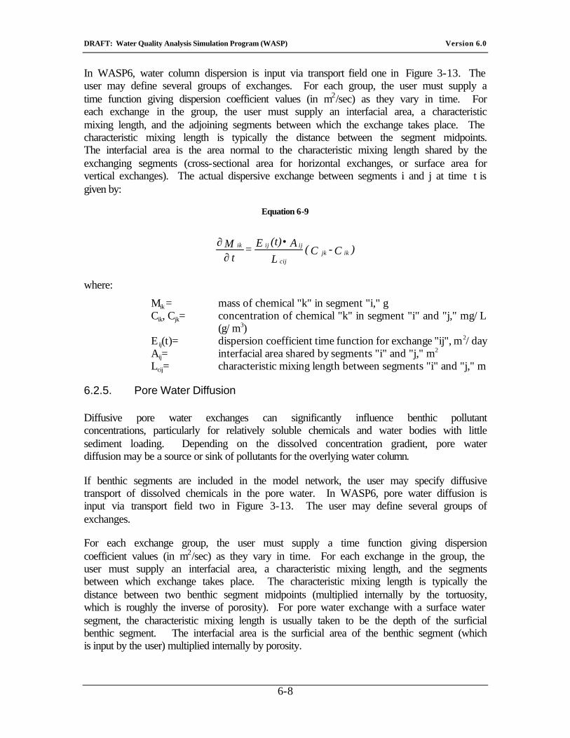
DRAFT: Water Quality Analysis Simulation Program (WASP) Version 6.0
6-8
In WASP6, water column dispersion is input via transport field one in Figure 3-13. The user may define several groups of exchanges. For each group, the user must supply a time function giving dispersion coefficient values (in m2/sec) as they vary in time. For each exchange in the group, the user must supply an interfacial area, a characteristic mixing length, and the adjoining segments between which the exchange takes place. The characteristic mixing length is typically the distance between the segment midpoints. The interfacial area is the area normal to the characteristic mixing length shared by the exchanging segments (cross-sectional area for horizontal exchanges, or surface area for vertical exchanges). The actual dispersive exchange between segments i and j at time t is given by:
Equation 6-9
)C - C( L
A (t) E = t
M ik jk
cij
ij ij ik •∂
∂
where:
Mik = mass of chemical "k" in segment "i," g Cik, Cjk= concentration of chemical "k" in segment "i" and "j," mg/L
(g/m3) Eij(t)= dispersion coefficient time function for exchange "ij", m2/day Aij= interfacial area shared by segments "i" and "j," m2 Lcij= characteristic mixing length between segments "i" and "j," m
6.2.5. Pore Water Diffusion
Diffusive pore water exchanges can significantly influence benthic pollutant concentrations, particularly for relatively soluble chemicals and water bodies with little sediment loading. Depending on the dissolved concentration gradient, pore water diffusion may be a source or sink of pollutants for the overlying water column.
If benthic segments are included in the model network, the user may specify diffusive transport of dissolved chemicals in the pore water. In WASP6, pore water diffusion is input via transport field two in Figure 3-13. The user may define several groups of exchanges.
For each exchange group, the user must supply a time function giving dispersion coefficient values (in m2/sec) as they vary in time. For each exchange in the group, the user must supply an interfacial area, a characteristic mixing length, and the segments between which exchange takes place. The characteristic mixing length is typically the distance between two benthic segment midpoints (multiplied internally by the tortuosity, which is roughly the inverse of porosity). For pore water exchange with a surface water segment, the characteristic mixing length is usually taken to be the depth of the surficial benthic segment. The interfacial area is the surficial area of the benthic segment (which is input by the user) multiplied internally by porosity.
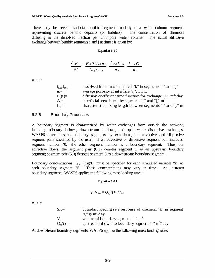
DRAFT: Water Quality Analysis Simulation Program (WASP) Version 6.0
6-9
There may be several surficial benthic segments underlying a water column segment, representing discrete benthic deposits (or habitats). The concentration of chemical diffusing is the dissolved fraction per unit pore water volume. The actual diffusive exchange between benthic segments i and j at time t is given by:
Equation 6-10
∂
∂n
C f -
n
C f
n/ Ln A (t) E =
t M
i
ik Dik
j
jk Djk
ij cij
ij ij ij ik
where:
fDik,fDjk = dissolved fraction of chemical "k" in segments "i" and "j" nij= average porosity at interface "ij", Lw/L Eij(t)= diffusion coefficient time function for exchange "ij", m2/day Aij= interfacial area shared by segments "i" and "j," m2 Lcij= characteristic mixing length between segments "i" and "j," m
6.2.6. Boundary Processes
A boundary segment is characterized by water exchanges from outside the network, including tributary inflows, downstream outflows, and open water dispersive exchanges. WASP6 determines its boundary segments by examining the advective and dispersive segment pairs specified by the user. If an advective or dispersive segment pair includes segment number "0," the other segment number is a boundary segment. Thus, for advective flows, the segment pair (0,1) denotes segment 1 as an upstream boundary segment; segment pair (5,0) denotes segment 5 as a downstream boundary segment.
Boundary concentrations CBik (mg/L) must be specified for each simulated variable "k" at each boundary segment "i". These concentrations may vary in time. At upstream boundary segments, WASP6 applies the following mass loading rates:
Equation 6-11
C (t)Q = S V Bik0iBiki •
where:
SBik= boundary loading rate response of chemical "k" in segment "i," g/m3-day
Vi= volume of boundary segment "i," m3 Q0i(t)= upstream inflow into boundary segment "i," m3/day
At downstream boundary segments, WASP6 applies the following mass loading rates:
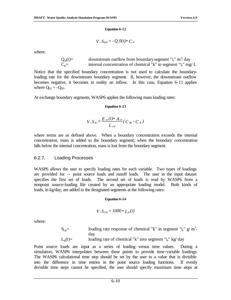
DRAFT: Water Quality Analysis Simulation Program (WASP) Version 6.0
6-10
Equation 6-12
C 0(t)Q - = S V ikiBiki •
where:
Qi0(t)= downstream outflow from boundary segment "i," m3/day Cik= internal concentration of chemical "k" in segment "i," mg/L
Notice that the specified boundary concentration is not used to calculate the boundary-loading rate for the downstream boundary segment. If, however, the downstream outflow becomes negative, it becomes in reality an inflow. In this case, Equation 6-11 applies where Q0i = -Qi0.
At exchange boundary segments, WASP6 applies the following mass loading rates:
Equation 6-13
)C - C( L
A (t) E = S V ik Bk ci0
i0 i0 Bii
•
where terms are as defined above. When a boundary concentration exceeds the internal concentration, mass is added to the boundary segment; when the boundary concentration falls below the internal concentration, mass is lost from the boundary segment.
6.2.7. Loading Processes
WASP6 allows the user to specify loading rates for each variable. Two types of loadings are provided for -- point source loads and runoff loads. The user in the input dataset specifies the first set of loads. The second set of loads is read by WASP6 from a nonpoint source-loading file created by an appropriate loading model. Both kinds of loads, in kg/day, are added to the designated segments at the following rates:
Equation 6-14
(t)L 1000 = S V ikLiki •
where:
SLik= loading rate response of chemical "k" in segment "i," g/m3-day
Lik(t)= loading rate of chemical "k" into segment "i," kg/day
Point source loads are input as a series of loading versus time values. During a simulation, WASP6 interpolates between these points to provide time-variable loadings. The WASP6 calculational time step should be set by the user to a value that is divisible into the difference in time entries in the point source loading functions. If evenly divisible time steps cannot be specified, the user should specify maximum time steps at
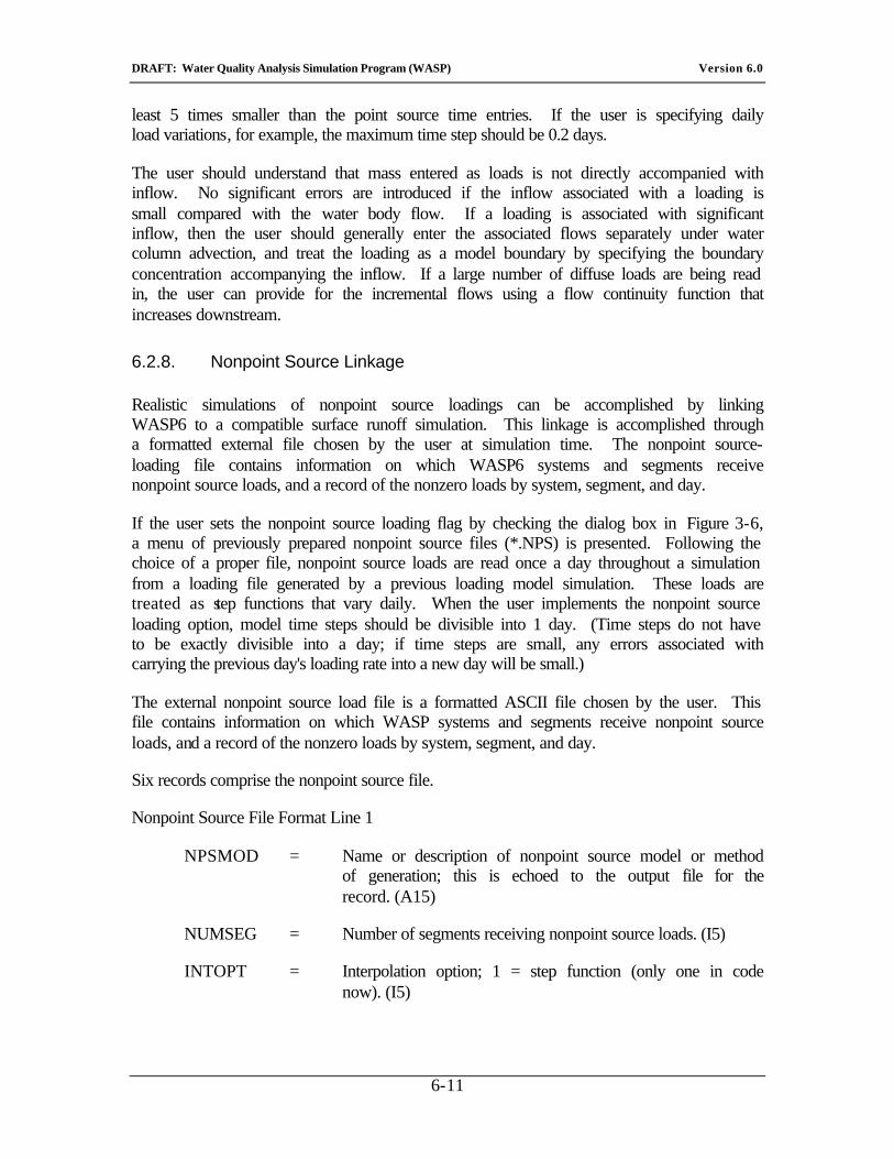
DRAFT: Water Quality Analysis Simulation Program (WASP) Version 6.0
6-11
least 5 times smaller than the point source time entries. If the user is specifying daily load variations, for example, the maximum time step should be 0.2 days.
The user should understand that mass entered as loads is not directly accompanied with inflow. No significant errors are introduced if the inflow associated with a loading is small compared with the water body flow. If a loading is associated with significant inflow, then the user should generally enter the associated flows separately under water column advection, and treat the loading as a model boundary by specifying the boundary concentration accompanying the inflow. If a large number of diffuse loads are being read in, the user can provide for the incremental flows using a flow continuity function that increases downstream.
6.2.8. Nonpoint Source Linkage
Realistic simulations of nonpoint source loadings can be accomplished by linking WASP6 to a compatible surface runoff simulation. This linkage is accomplished through a formatted external file chosen by the user at simulation time. The nonpoint source-loading file contains information on which WASP6 systems and segments receive nonpoint source loads, and a record of the nonzero loads by system, segment, and day.
If the user sets the nonpoint source loading flag by checking the dialog box in Figure 3-6, a menu of previously prepared nonpoint source files (*.NPS) is presented. Following the choice of a proper file, nonpoint source loads are read once a day throughout a simulation from a loading file generated by a previous loading model simulation. These loads are treated as step functions that vary daily. When the user implements the nonpoint source loading option, model time steps should be divisible into 1 day. (Time steps do not have to be exactly divisible into a day; if time steps are small, any errors associated with carrying the previous day's loading rate into a new day will be small.)
The external nonpoint source load file is a formatted ASCII file chosen by the user. This file contains information on which WASP systems and segments receive nonpoint source loads, and a record of the nonzero loads by system, segment, and day.
Six records comprise the nonpoint source file.
Nonpoint Source File Format Line 1
NPSMOD = Name or description of nonpoint source model or method of generation; this is echoed to the output file for the record. (A15)
NUMSEG = Number of segments receiving nonpoint source loads. (I5)
INTOPT = Interpolation option; 1 = step function (only one in code now). (I5)
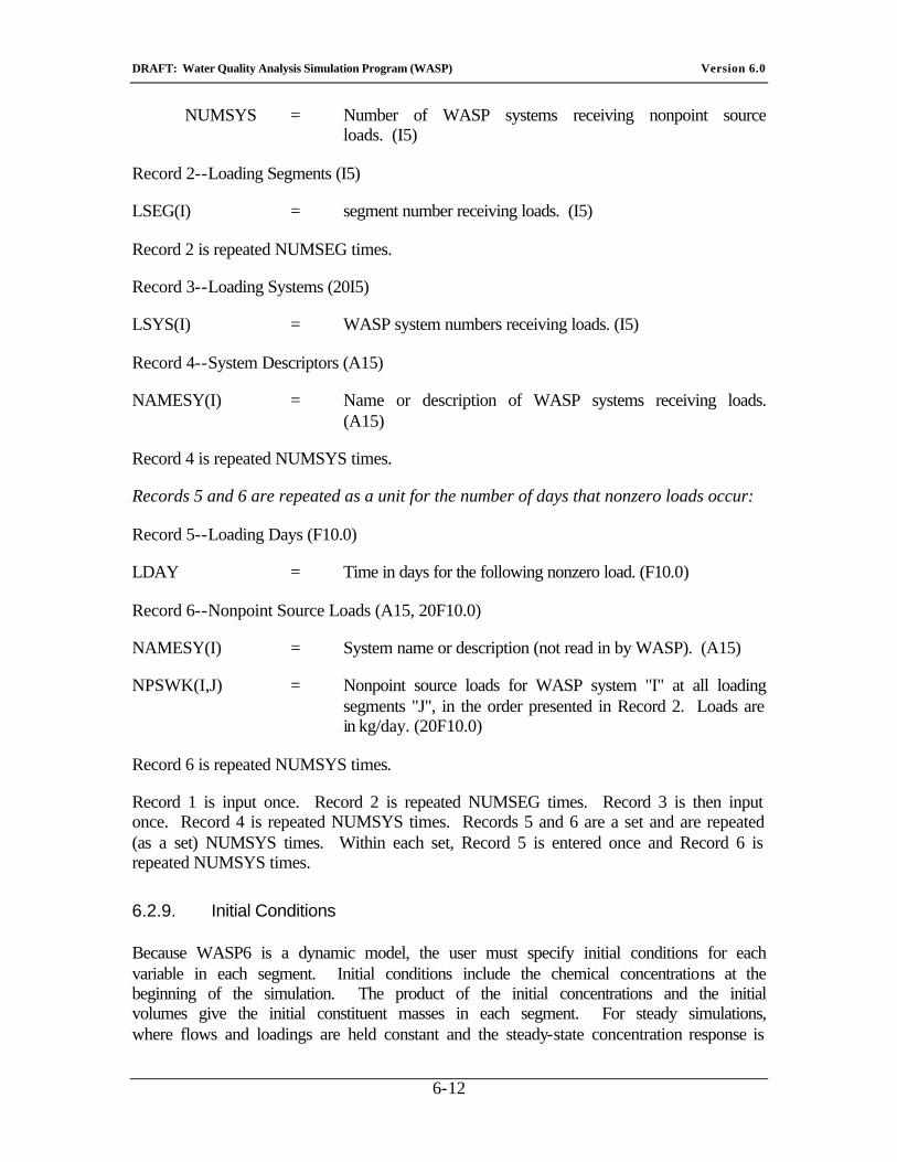
DRAFT: Water Quality Analysis Simulation Program (WASP) Version 6.0
6-12
NUMSYS = Number of WASP systems receiving nonpoint source loads. (I5)
Record 2--Loading Segments (I5)
LSEG(I) = segment number receiving loads. (I5)
Record 2 is repeated NUMSEG times.
Record 3--Loading Systems (20I5)
LSYS(I) = WASP system numbers receiving loads. (I5)
Record 4--System Descriptors (A15)
NAMESY(I) = Name or description of WASP systems receiving loads. (A15)
Record 4 is repeated NUMSYS times.
Records 5 and 6 are repeated as a unit for the number of days that nonzero loads occur:
Record 5--Loading Days (F10.0)
LDAY = Time in days for the following nonzero load. (F10.0)
Record 6--Nonpoint Source Loads (A15, 20F10.0)
NAMESY(I) = System name or description (not read in by WASP). (A15)
NPSWK(I,J) = Nonpoint source loads for WASP system "I" at all loading segments "J", in the order presented in Record 2. Loads are in kg/day. (20F10.0)
Record 6 is repeated NUMSYS times.
Record 1 is input once. Record 2 is repeated NUMSEG times. Record 3 is then input once. Record 4 is repeated NUMSYS times. Records 5 and 6 are a set and are repeated (as a set) NUMSYS times. Within each set, Record 5 is entered once and Record 6 is repeated NUMSYS times.
6.2.9. Initial Conditions
Because WASP6 is a dynamic model, the user must specify initial conditions for each variable in each segment. Initial conditions include the chemical concentrations at the beginning of the simulation. The product of the initial concentrations and the initial volumes give the initial constituent masses in each segment. For steady simulations, where flows and loadings are held constant and the steady-state concentration response is
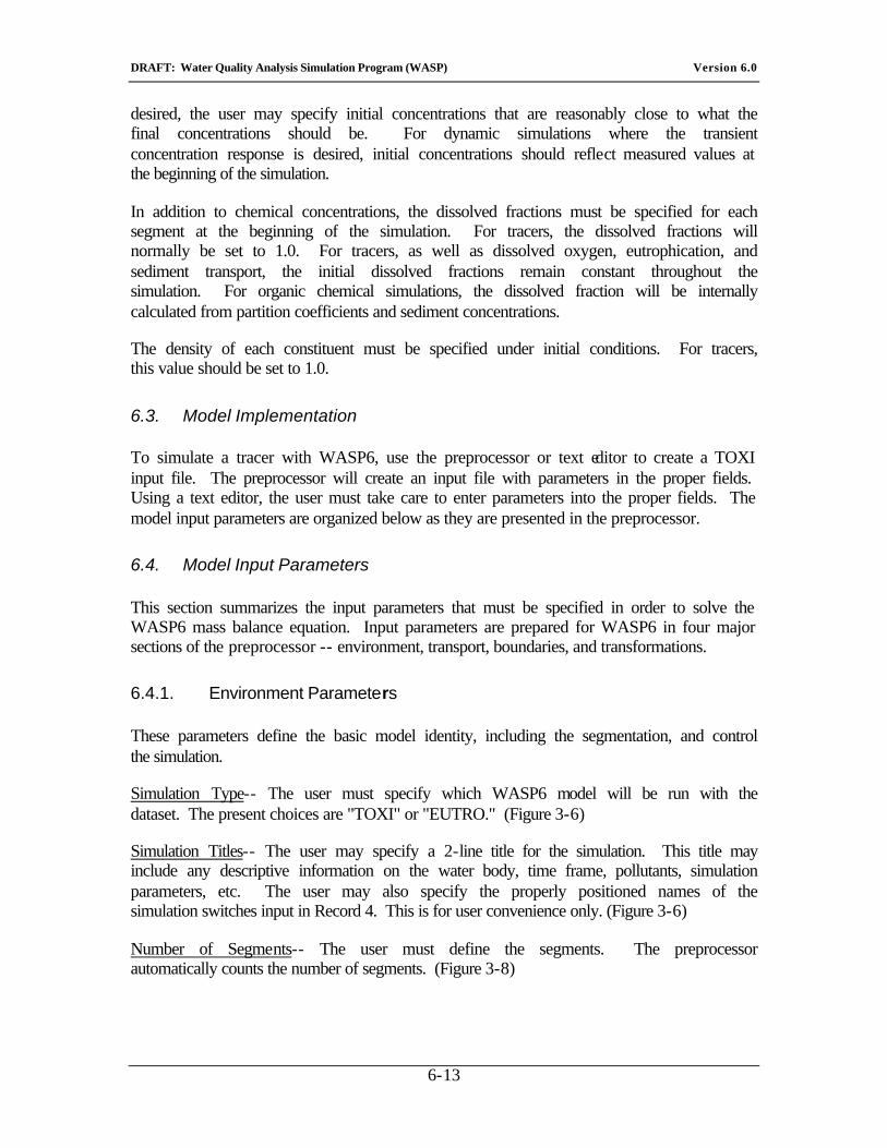
DRAFT: Water Quality Analysis Simulation Program (WASP) Version 6.0
6-13
desired, the user may specify initial concentrations that are reasonably close to what the final concentrations should be. For dynamic simulations where the transient concentration response is desired, initial concentrations should reflect measured values at the beginning of the simulation.
In addition to chemical concentrations, the dissolved fractions must be specified for each segment at the beginning of the simulation. For tracers, the dissolved fractions will normally be set to 1.0. For tracers, as well as dissolved oxygen, eutrophication, and sediment transport, the initial dissolved fractions remain constant throughout the simulation. For organic chemical simulations, the dissolved fraction will be internally calculated from partition coefficients and sediment concentrations.
The density of each constituent must be specified under initial conditions. For tracers, this value should be set to 1.0.
6.3. Model Implementation
To simulate a tracer with WASP6, use the preprocessor or text editor to create a TOXI input file. The preprocessor will create an input file with parameters in the proper fields. Using a text editor, the user must take care to enter parameters into the proper fields. The model input parameters are organized below as they are presented in the preprocessor.
6.4. Model Input Parameters
This section summarizes the input parameters that must be specified in order to solve the WASP6 mass balance equation. Input parameters are prepared for WASP6 in four major sections of the preprocessor -- environment, transport, boundaries, and transformations.
6.4.1. Environment Parameters
These parameters define the basic model identity, including the segmentation, and control the simulation.
Simulation Type-- The user must specify which WASP6 model will be run with the dataset. The present choices are "TOXI" or "EUTRO." (Figure 3-6)
Simulation Titles-- The user may specify a 2-line title for the simulation. This title may include any descriptive information on the water body, time frame, pollutants, simulation parameters, etc. The user may also specify the properly positioned names of the simulation switches input in Record 4. This is for user convenience only. (Figure 3-6)
Number of Segments-- The user must define the segments. The preprocessor automatically counts the number of segments. (Figure 3-8)
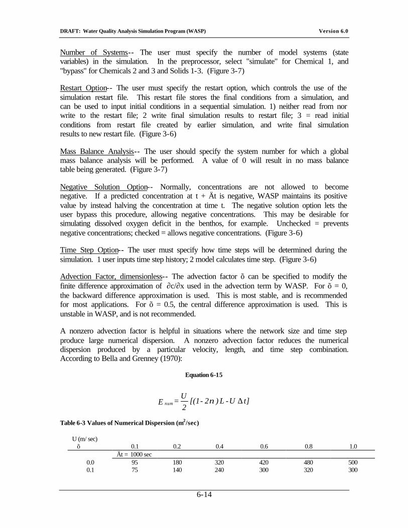
DRAFT: Water Quality Analysis Simulation Program (WASP) Version 6.0
6-14
Number of Systems-- The user must specify the number of model systems (state variables) in the simulation. In the preprocessor, select "simulate" for Chemical 1, and "bypass" for Chemicals 2 and 3 and Solids 1-3. (Figure 3-7)
Restart Option-- The user must specify the restart option, which controls the use of the simulation restart file. This restart file stores the final conditions from a simulation, and can be used to input initial conditions in a sequential simulation. 1) neither read from nor write to the restart file; 2 write final simulation results to restart file; 3 = read initial conditions from restart file created by earlier simulation, and write final simulation results to new restart file. (Figure 3-6)
Mass Balance Analysis-- The user should specify the system number for which a global mass balance analysis will be performed. A value of 0 will result in no mass balance table being generated. (Figure 3-7)
Negative Solution Option-- Normally, concentrations are not allowed to become negative. If a predicted concentration at t + Ät is negative, WASP maintains its positive value by instead halving the concentration at time t. The negative solution option lets the user bypass this procedure, allowing negative concentrations. This may be desirable for simulating dissolved oxygen deficit in the benthos, for example. Unchecked = prevents negative concentrations; checked = allows negative concentrations. (Figure 3-6)
Time Step Option-- The user must specify how time steps will be determined during the simulation. 1 user inputs time step history; 2 model calculates time step. (Figure 3-6)
Advection Factor, dimensionless-- The advection factor õ can be specified to modify the finite difference approximation of ∂c/∂x used in the advection term by WASP. For õ = 0, the backward difference approximation is used. This is most stable, and is recommended for most applications. For õ = 0.5, the central difference approximation is used. This is unstable in WASP, and is not recommended.
A nonzero advection factor is helpful in situations where the network size and time step produce large numerical dispersion. A nonzero advection factor reduces the numerical dispersion produced by a particular velocity, length, and time step combination. According to Bella and Grenney (1970):
Equation 6-15
t] U - L ) 2 - [(1 2U = E num ∆ν
Table 6-3 Values of Numerical Dispersion (m2/sec)
U (m/sec) õ 0.1 0.2 0.4 0.6 0.8 1.0 Ät = 1000 sec
0.0 95 180 320 420 480 500 0.1 75 140 240 300 320 300
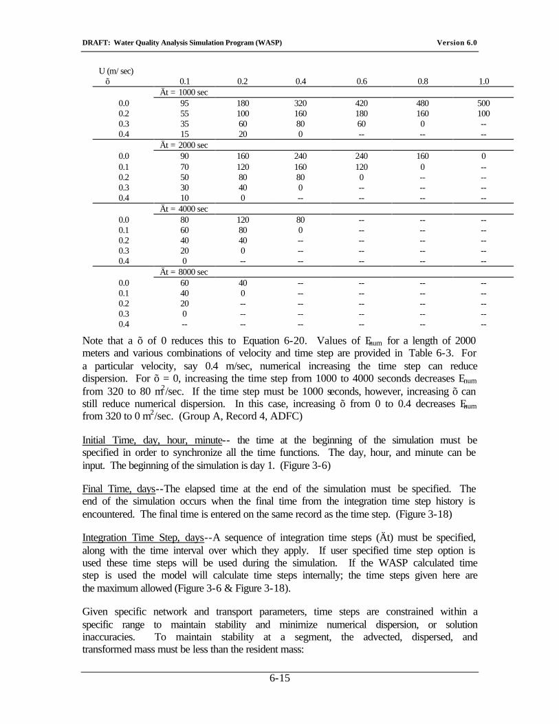
DRAFT: Water Quality Analysis Simulation Program (WASP) Version 6.0
6-15
U (m/sec) õ 0.1 0.2 0.4 0.6 0.8 1.0 Ät = 1000 sec
0.0 95 180 320 420 480 500 0.2 55 100 160 180 160 100 0.3 35 60 80 60 0 -- 0.4 15 20 0 -- -- --
Ät = 2000 sec 0.0 90 160 240 240 160 0 0.1 70 120 160 120 0 -- 0.2 50 80 80 0 -- -- 0.3 30 40 0 -- -- -- 0.4 10 0 -- -- -- --
Ät = 4000 sec 0.0 80 120 80 -- -- -- 0.1 60 80 0 -- -- -- 0.2 40 40 -- -- -- -- 0.3 20 0 -- -- -- -- 0.4 0 -- -- -- -- --
Ät = 8000 sec 0.0 60 40 -- -- -- -- 0.1 40 0 -- -- -- -- 0.2 20 -- -- -- -- -- 0.3 0 -- -- -- -- -- 0.4 -- -- -- -- -- --
Note that a õ of 0 reduces this to Equation 6-20. Values of Enum for a length of 2000 meters and various combinations of velocity and time step are provided in Table 6-3. For a particular velocity, say 0.4 m/sec, numerical increasing the time step can reduce dispersion. For õ = 0, increasing the time step from 1000 to 4000 seconds decreases Enum from 320 to 80 m2/sec. If the time step must be 1000 seconds, however, increasing õ can still reduce numerical dispersion. In this case, increasing õ from 0 to 0.4 decreases Enum from 320 to 0 m2/sec. (Group A, Record 4, ADFC)
Initial Time, day, hour, minute-- the time at the beginning of the simulation must be specified in order to synchronize all the time functions. The day, hour, and minute can be input. The beginning of the simulation is day 1. (Figure 3-6)
Final Time, days--The elapsed time at the end of the simulation must be specified. The end of the simulation occurs when the final time from the integration time step history is encountered. The final time is entered on the same record as the time step. (Figure 3-18)
Integration Time Step, days--A sequence of integration time steps (Ät) must be specified, along with the time interval over which they apply. If user specified time step option is used these time steps will be used during the simulation. If the WASP calculated time step is used the model will calculate time steps internally; the time steps given here are the maximum allowed (Figure 3-6 & Figure 3-18).
Given specific network and transport parameters, time steps are constrained within a specific range to maintain stability and minimize numerical dispersion, or solution inaccuracies. To maintain stability at a segment, the advected, dispersed, and transformed mass must be less than the resident mass:
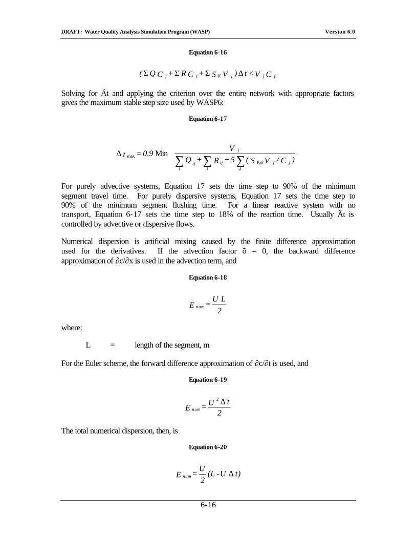
DRAFT: Water Quality Analysis Simulation Program (WASP) Version 6.0
6-16
Equation 6-16
C V < t )V S + C R + C Q ( j j j K j j ∆ΣΣΣ
Solving for Ät and applying the criterion over the entire network with appropriate factors gives the maximum stable step size used by WASP6:
Equation 6-17
∆
∑∑∑ )C/ V S( 5 + R + Q V
0.9 = t j j Kjk
kij
iij
i
j Minmax
For purely advective systems, Equation 17 sets the time step to 90% of the minimum segment travel time. For purely dispersive systems, Equation 17 sets the time step to 90% of the minimum segment flushing time. For a linear reactive system with no transport, Equation 6-17 sets the time step to 18% of the reaction time. Usually Ät is controlled by advective or dispersive flows.
Numerical dispersion is artificial mixing caused by the finite difference approximation used for the derivatives. If the advection factor õ = 0, the backward difference approximation of ∂c/∂x is used in the advection term, and
Equation 6-18
2L U
= E num
where:
L = length of the segment, m
For the Euler scheme, the forward difference approximation of ∂c/∂t is used, and
Equation 6-19
2t U = E
2
num ∆
The total numerical dispersion, then, is
Equation 6-20
t) U - (L 2U = E num ∆
DRAFT: Water Quality Analysis Simulation Program (WASP) Version 6.0
6-17
Note that increasing the time step up to Äx/U (or V/Q) decreases numerical dispersion to 0. The conditions for stability discussed above require a time step somewhat less than V/Q for most segments. So to maintain stability and minimize numerical dispersion in a water body subject to unsteady flow, the sequence of time steps must be as large as possible, but always less than Ätmax given in Equation 6-17. (Figure 3-18)
Print Intervals, days-- The user must specify the print intervals controlling the output density in the print file transferred to the post-processor. The model will store all display variables in all segments after each print interval throughout the simulation. Different print intervals can be specified for different phases in the simulation. At least two print intervals must be specified, one for time 0 and one for the final time. (Figure 3-19)
Segment Volumes, m3--Initial volumes for each segment must be specified. These can be calculated from navigation charts or from a series of transects measuring depth versus width along the river. Sometimes, volumes can be estimated from the travel time of a well-mixed cloud of dye through a reach. For simulations using hydrodynamic results, volumes from the hydrodynamic summary file (#.HYD) are used and continuity is maintained. (Figure 3-8)
6.4.2. Transport Parameters
This group of parameters defines the advective and dispersive transport of simulated model variables. Input parameters include advective flows, sediment transport velocities, dispersion coefficients, cross-sectional areas, and characteristic lengths. Although the nominal units expected by the model are SI, English or other units can be used along with proper specification of conversion factors.
Advective Flow, m3/sec--Steady or unsteady flows can be specified between adjoining segments, as well as entering or leaving the network as inflow or outflow. The user must be careful to check for continuity errors, as the model does not require that flow continuity be maintained. For example, the user may specify that more flow enter a segment than leaves. For simulations using hydrodynamic results from the *.HYD file flow continuity is automatically maintained. (Figure 3-14)
Dispersion Coefficients, m2/sec--Dispersive mixing coefficients can be specified between adjoining segments, or across open water boundaries. These coefficients can model pore water diffusion in benthic segments, vertical diffusion in lakes, and lateral and longitudinal dispersion in large water bodies. Values can range from 10-10 m2/sec for molecular diffusion to 5x10² m2/sec for longitudinal mixing in some estuaries. Values are entered as a time function series of dispersion and time, in days. (Figure 3-13)
Cross-Sectional Area, m2--Cross-sectional areas are specified for each dispersion coefficient, reflecting the area through which mixing occurs. These can be surface areas for vertical exchange, such as in lakes or in the benthos. Areas are not modified during the simulation to reflect flow changes. (Figure 3-13)
DRAFT: Water Quality Analysis Simulation Program (WASP) Version 6.0
6-18
Characteristic Mixing Length, m--Mixing lengths are specified for each dispersion coefficient, reflecting the characteristic length over which mixing occurs. These are typically the lengths between the center points of adjoining segments. A single segment may have three or more mixing lengths for segments adjoining longitudinally, laterally, and vertically. For surficial benthic segments connecting water column segments, the depth of the benthic layer is a more realistic mixing length than half the water depth. (Figure 3-13)
6.4.3. Boundary Parameters
This group of parameters includes boundary concentrations, waste loads, and initial conditions. Boundary concentrations must be specified for any segment receiving flow inputs, outputs, or exchanges. Initial conditions include not only initial concentrations, but also the density and solids transport field for each solid, and the dissolved fraction in each segment.
Boundary Concentrations, mg/L--Steady or time-variable concentrations must be specified for each water quality constituent at each boundary. A boundary is a tributary inflow, a downstream outflow, or an open water end of the model network across which dispersive mixing can occur. Advective and dispersive flows across boundaries are specified by the transport parameters. Values are entered as a time function series of concentrations and time, in days. (Figure 3-15)
Waste Loads, kg/day--Steady or time-variable loads may be specified for each water quality constituent at several segments. These loads represent municipal and industrial wastewater discharges, urban and agricultural runoff, precipitation, and atmospheric deposition of pollutants. Values are entered as a time function series of loads and time, in days. (Figure 3-16)
Initial Concentrations, mg/L--Concentrations of each constituent in each segment must be specified for the time at which the simulation begins. For those water bodies with low transport rates, the initial concentrations of conservative substances may persist for a long period of time. Accurate simulation, then, would require accurate specification of initial concentrations. If initial concentrations cannot be determined accurately, then longer simulations should be run, and early predictions discounted. (Figure 3-10)
Dissolved Fractions--The initial fraction of chemical dissolved in the water portion of a segment is input as a fraction of total chemical concentration. The dissolved fraction is important in determining the amount of chemical transported by pore water flow and dispersion, and by solids transport. Dissolved fractions may be computed from sorption kinetics in the transformation subroutines. (Figure 3-11)
Solid Densities, g/cm3--The density of each type of solid is needed to compute the porosity of bed segments. Porosity will be a function of sediment concentration and the density of each solid type. (Figure 3-7)
DRAFT: Water Quality Analysis Simulation Program (WASP) Version 6.0
6-19
Maximum Concentrations, mg/L--Maximum concentrations must be specified for each water quality constituent. The simulation is automatically aborted if a calculated concentration falls outside these limits. This usually indicates computational instability, and the time step must usually be reduced. (Figure 3-7)
6.4.4. Transformation Parameters
This group of parameters includes spatially variable parameters, constants, and kinetic time functions for the water quality constituents being simulated. None are necessary for dissolved, conservative chemicals.
6.4.5. External Input Files
At the user's option, two external input files may be called upon and used by WASP6 during a simulation. These formatted files may be created by a simulation model, or by output from a spreadsheet. As formatted ASCII files, they may be edited using standard text editors. Hydrodynamic files are denoted by *.HYD, where the user specifies a 1 to 8 character name for *. Nonpoint source loading files are denoted by *.NPS. The contents and format for these files are specified on page 3-13.
DRAFT: Water Quality Analysis Simulation Program (WASP) Version 6.0
7-1
7. Sediment Transport
Sediment transport is potentially a very important process in aquatic systems. Excess sediment can affect water quality directly. Water clarity and benthic habitats can be degraded. Sediment transport also influences chemical transport and fate. Many chemicals sorb strongly to sediment and thus undergo settling, scour, and sedimentation. Sorption also affects a chemical's transfer and transformation rates. Volatilization and base-catalyzed hydrolysis, for example, are slowed by sorption. Both sediment transport rates and concentrations must be estimated in most toxic chemical studies.
In general, the stream transport capacity for suspended sediment is in excess of its actual load, and the problem is one of estimating sediment source loading--namely, watershed erosion. In areas of backwater behind dams or in sluggish reaches, the stream transport capacity may drop enough to allow net deposition. Strongly sorbed pollutants may build up significantly. Because sediment transport can be complex, site-specific calibration of the settling, scour, and sedimentation rates is usually necessary.
7.1. Overview of WASP Sediment Transport
Sediment size fractions, or solids types, are simulated using the TOXI program. Simulations may incorporate total solids as a single variable, or, alternately, represent from one to three solids types or fractions. The character of the three solids types is user-defined. They may represent sand, silt, and clay, or organic solids and inorganic solids. The user defines each solid type by specifying its settling and erosion rates, and its organic content.
WASP6 performs a simple mass balance on each solid variable in each compartment based upon specified water column advection and dispersion rates, along with special settling, deposition, erosion, burial, and bed load rates. Mass balance computations are performed in benthic compartments as well as water column compartments. Bulk densities or benthic volumes are adjusted throughout the simulation.
The user can vary all solids transport rates in space and time. There are, however, no special process descriptions for solids transport. Erosion rates, for example, are not programmed as a function of sediment shear strength and water column shear stress. Consequently, the TOXI sediment model should be considered descriptive, and must be calibrated to site data.
7.1.1. Sediment Transport Processes
Water Column Transport
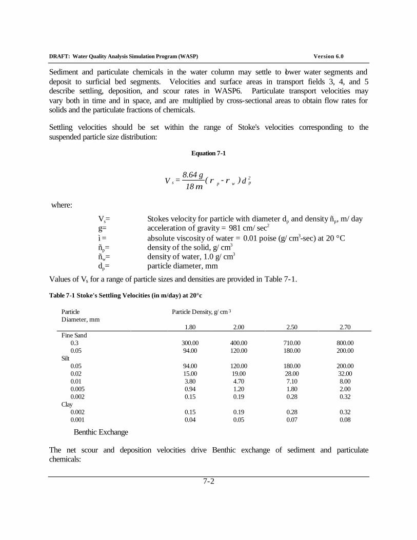
DRAFT: Water Quality Analysis Simulation Program (WASP) Version 6.0
7-2
Sediment and particulate chemicals in the water column may settle to lower water segments and deposit to surficial bed segments. Velocities and surface areas in transport fields 3, 4, and 5 describe settling, deposition, and scour rates in WASP6. Particulate transport velocities may vary both in time and in space, and are multiplied by cross-sectional areas to obtain flow rates for solids and the particulate fractions of chemicals.
Settling velocities should be set within the range of Stoke's velocities corresponding to the suspended particle size distribution:
Equation 7-1
d ) - ( 18
g 8.64 = V 2
p wp s ρρµ
where:
Vs= Stokes velocity for particle with diameter dp and density ñp, m/day g= acceleration of gravity = 981 cm/sec2 ì= absolute viscosity of water = 0.01 poise (g/cm3-sec) at 20 °C ñp= density of the solid, g/cm3 ñw= density of water, 1.0 g/cm3 dp= particle diameter, mm
Values of Vs for a range of particle sizes and densities are provided in Table 7-1.
Table 7-1 Stoke's Settling Velocities (in m/day) at 20°c
Particle Diameter, mm
Particle Density, g/cm 3
1.80 2.00 2.50 2.70 Fine Sand 0.3 300.00 400.00 710.00 800.00 0.05 94.00 120.00 180.00 200.00 Silt 0.05 94.00 120.00 180.00 200.00 0.02 15.00 19.00 28.00 32.00 0.01 3.80 4.70 7.10 8.00 0.005 0.94 1.20 1.80 2.00 0.002 0.15 0.19 0.28 0.32 Clay 0.002 0.15 0.19 0.28 0.32 0.001 0.04 0.05 0.07 0.08
Benthic Exchange
The net scour and deposition velocities drive Benthic exchange of sediment and particulate chemicals:
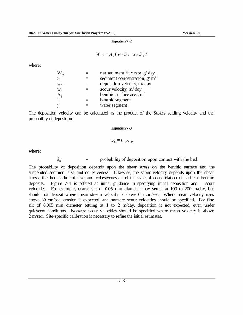
DRAFT: Water Quality Analysis Simulation Program (WASP) Version 6.0
7-3
Equation 7-2
)S w - S w( A = W j D i R ij Bs
where:
WBs = net sediment flux rate, g/day S = sediment concentration, g/m3 wD = deposition velocity, m/day wR = scour velocity, m/day Aij = benthic surface area, m2 i = benthic segment j = water segment
The deposition velocity can be calculated as the product of the Stokes settling velocity and the probability of deposition:
Equation 7-3
α D sD V = w
where:
áD = probability of deposition upon contact with the bed.
The probability of deposition depends upon the shear stress on the benthic surface and the suspended sediment size and cohesiveness. Likewise, the scour velocity depends upon the shear stress, the bed sediment size and cohesiveness, and the state of consolidation of surficial benthic deposits. Figure 7-1 is offered as initial guidance in specifying initial deposition and scour velocities. For example, coarse silt of 0.05 mm diameter may settle at 100 to 200 m/day, but should not deposit where mean stream velocity is above 0.5 cm/sec. Where mean velocity rises above 30 cm/sec, erosion is expected, and nonzero scour velocities should be specified. For fine silt of 0.005 mm diameter settling at 1 to 2 m/day, deposition is not expected, even under quiescent conditions. Nonzero scour velocities should be specified where mean velocity is above 2 m/sec. Site-specific calibration is necessary to refine the initial estimates.
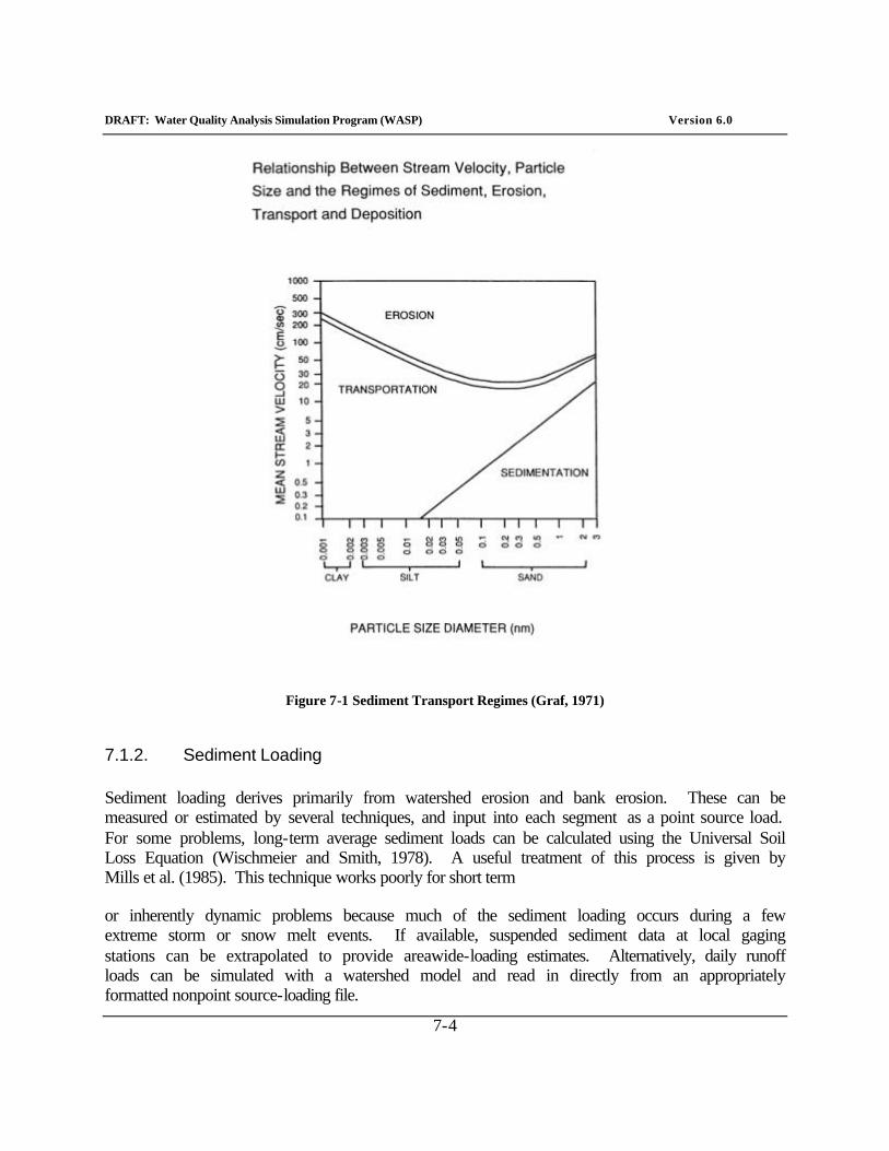
DRAFT: Water Quality Analysis Simulation Program (WASP) Version 6.0
7-4
Figure 7-1 Sediment Transport Regimes (Graf, 1971)
7.1.2. Sediment Loading
Sediment loading derives primarily from watershed erosion and bank erosion. These can be measured or estimated by several techniques, and input into each segment as a point source load. For some problems, long-term average sediment loads can be calculated using the Universal Soil Loss Equation (Wischmeier and Smith, 1978). A useful treatment of this process is given by Mills et al. (1985). This technique works poorly for short term
or inherently dynamic problems because much of the sediment loading occurs during a few extreme storm or snow melt events. If available, suspended sediment data at local gaging stations can be extrapolated to provide areawide-loading estimates. Alternatively, daily runoff loads can be simulated with a watershed model and read in directly from an appropriately formatted nonpoint source-loading file.
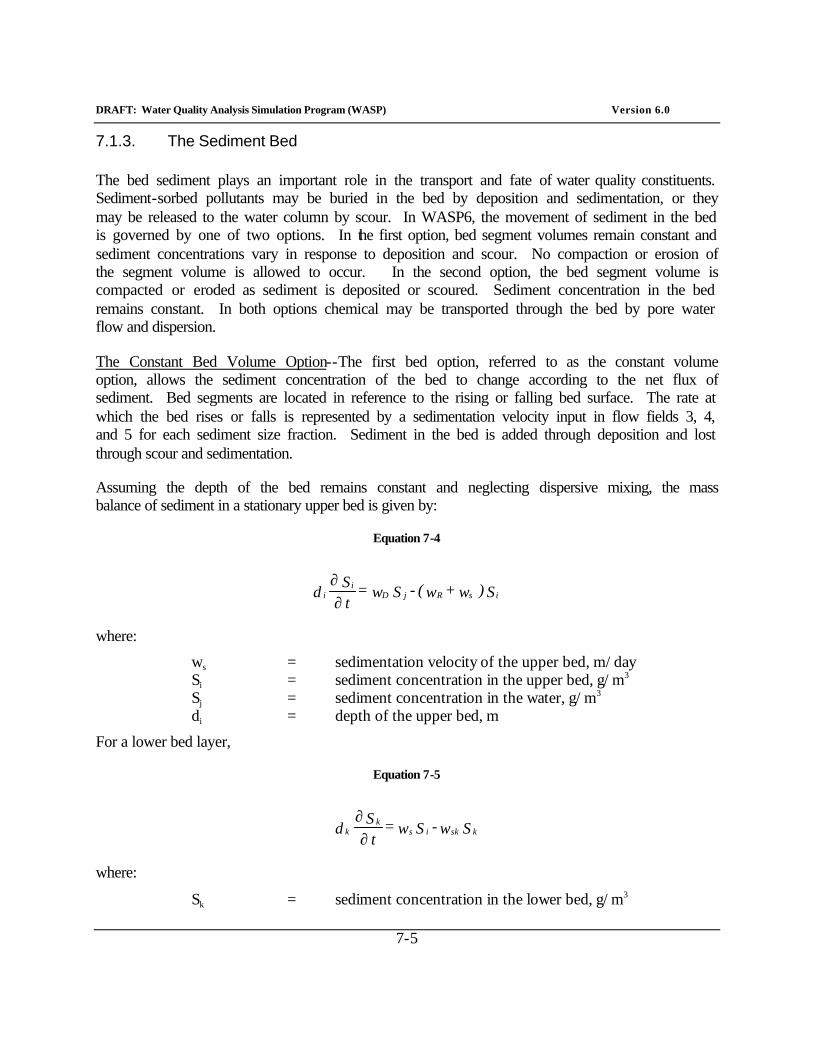
DRAFT: Water Quality Analysis Simulation Program (WASP) Version 6.0
7-5
7.1.3. The Sediment Bed
The bed sediment plays an important role in the transport and fate of water quality constituents. Sediment-sorbed pollutants may be buried in the bed by deposition and sedimentation, or they may be released to the water column by scour. In WASP6, the movement of sediment in the bed is governed by one of two options. In the first option, bed segment volumes remain constant and sediment concentrations vary in response to deposition and scour. No compaction or erosion of the segment volume is allowed to occur. In the second option, the bed segment volume is compacted or eroded as sediment is deposited or scoured. Sediment concentration in the bed remains constant. In both options chemical may be transported through the bed by pore water flow and dispersion.
The Constant Bed Volume Option--The first bed option, referred to as the constant volume option, allows the sediment concentration of the bed to change according to the net flux of sediment. Bed segments are located in reference to the rising or falling bed surface. The rate at which the bed rises or falls is represented by a sedimentation velocity input in flow fields 3, 4, and 5 for each sediment size fraction. Sediment in the bed is added through deposition and lost through scour and sedimentation.
Assuming the depth of the bed remains constant and neglecting dispersive mixing, the mass balance of sediment in a stationary upper bed is given by:
Equation 7-4
S ) w + w( - S w = t S d isRjD
ii ∂∂
where:
ws = sedimentation velocity of the upper bed, m/day Si = sediment concentration in the upper bed, g/m3 Sj = sediment concentration in the water, g/m3 di = depth of the upper bed, m
For a lower bed layer,
Equation 7-5
S w - S w = t
S d kskisk
k ∂∂
where:
Sk = sediment concentration in the lower bed, g/m3
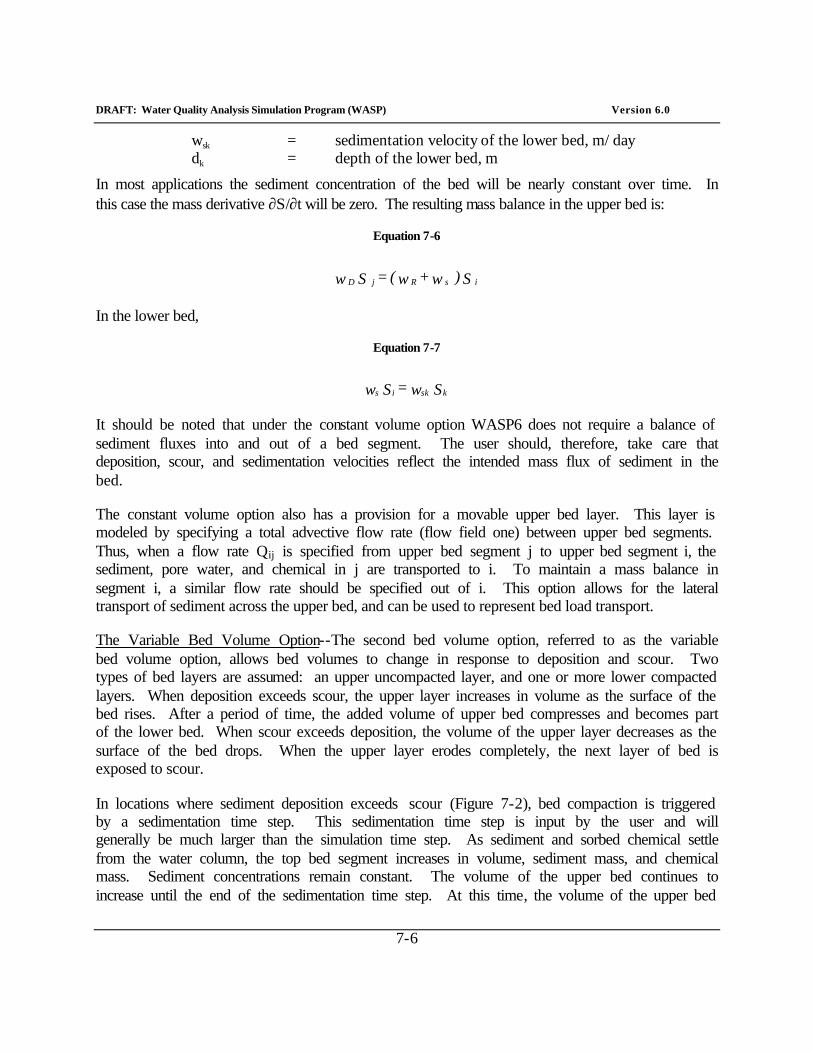
DRAFT: Water Quality Analysis Simulation Program (WASP) Version 6.0
7-6
wsk = sedimentation velocity of the lower bed, m/day dk = depth of the lower bed, m
In most applications the sediment concentration of the bed will be nearly constant over time. In this case the mass derivative ∂S/∂t will be zero. The resulting mass balance in the upper bed is:
Equation 7-6
S ) w + w( = S w i sR j D
In the lower bed,
Equation 7-7
S w = S w kskis
It should be noted that under the constant volume option WASP6 does not require a balance of sediment fluxes into and out of a bed segment. The user should, therefore, take care that deposition, scour, and sedimentation velocities reflect the intended mass flux of sediment in the bed.
The constant volume option also has a provision for a movable upper bed layer. This layer is modeled by specifying a total advective flow rate (flow field one) between upper bed segments. Thus, when a flow rate Qij is specified from upper bed segment j to upper bed segment i, the sediment, pore water, and chemical in j are transported to i. To maintain a mass balance in segment i, a similar flow rate should be specified out of i. This option allows for the lateral transport of sediment across the upper bed, and can be used to represent bed load transport.
The Variable Bed Volume Option--The second bed volume option, referred to as the variable bed volume option, allows bed volumes to change in response to deposition and scour. Two types of bed layers are assumed: an upper uncompacted layer, and one or more lower compacted layers. When deposition exceeds scour, the upper layer increases in volume as the surface of the bed rises. After a period of time, the added volume of upper bed compresses and becomes part of the lower bed. When scour exceeds deposition, the volume of the upper layer decreases as the surface of the bed drops. When the upper layer erodes completely, the next layer of bed is exposed to scour.
In locations where sediment deposition exceeds scour (Figure 7-2), bed compaction is triggered by a sedimentation time step. This sedimentation time step is input by the user and will generally be much larger than the simulation time step. As sediment and sorbed chemical settle from the water column, the top bed segment increases in volume, sediment mass, and chemical mass. Sediment concentrations remain constant. The volume of the upper bed continues to increase until the end of the sedimentation time step. At this time, the volume of the upper bed
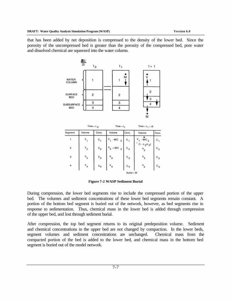
DRAFT: Water Quality Analysis Simulation Program (WASP) Version 6.0
7-7
that has been added by net deposition is compressed to the density of the lower bed. Since the porosity of the uncompressed bed is greater than the porosity of the compressed bed, pore water and dissolved chemical are squeezed into the water column.
Figure 7-2 WASP Sediment Burial
During compression, the lower bed segments rise to include the compressed portion of the upper bed. The volumes and sediment concentrations of these lower bed segments remain constant. A portion of the bottom bed segment is buried out of the network, however, as bed segments rise in response to sedimentation. Thus, chemical mass in the lower bed is added through compression of the upper bed, and lost through sediment burial.
After compression, the top bed segment returns to its original predeposition volume. Sediment and chemical concentrations in the upper bed are not changed by compaction. In the lower beds, segment volumes and sediment concentrations are unchanged. Chemical mass from the compacted portion of the bed is added to the lower bed, and chemical mass in the bottom bed segment is buried out of the model network.
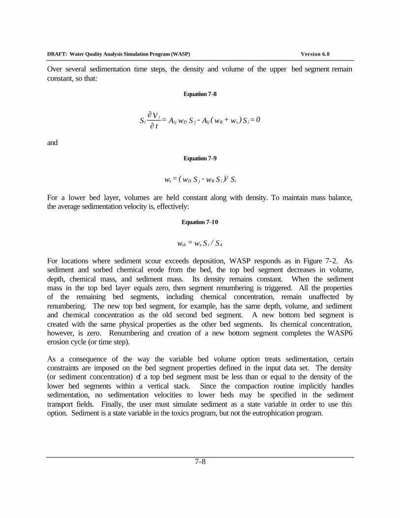
DRAFT: Water Quality Analysis Simulation Program (WASP) Version 6.0
7-8
Over several sedimentation time steps, the density and volume of the upper bed segment remain constant, so that:
Equation 7-8
0 = S )w + w( A - S w A = t
V S isRijjDiji
i ∂∂
and
Equation 7-9
S)/S w - S w( = w iiRjDs
For a lower bed layer, volumes are held constant along with density. To maintain mass balance, the average sedimentation velocity is, effectively:
Equation 7-10
S/S w = w kissk
For locations where sediment scour exceeds deposition, WASP responds as in Figure 7-2. As sediment and sorbed chemical erode from the bed, the top bed segment decreases in volume, depth, chemical mass, and sediment mass. Its density remains constant. When the sediment mass in the top bed layer equals zero, then segment renumbering is triggered. All the properties of the remaining bed segments, including chemical concentration, remain unaffected by renumbering. The new top bed segment, for example, has the same depth, volume, and sediment and chemical concentration as the old second bed segment. A new bottom bed segment is created with the same physical properties as the other bed segments. Its chemical concentration, however, is zero. Renumbering and creation of a new bottom segment completes the WASP6 erosion cycle (or time step).
As a consequence of the way the variable bed volume option treats sedimentation, certain constraints are imposed on the bed segment properties defined in the input data set. The density (or sediment concentration) of a top bed segment must be less than or equal to the density of the lower bed segments within a vertical stack. Since the compaction routine implicitly handles sedimentation, no sedimentation velocities to lower beds may be specified in the sediment transport fields. Finally, the user must simulate sediment as a state variable in order to use this option. Sediment is a state variable in the toxics program, but not the eutrophication program.
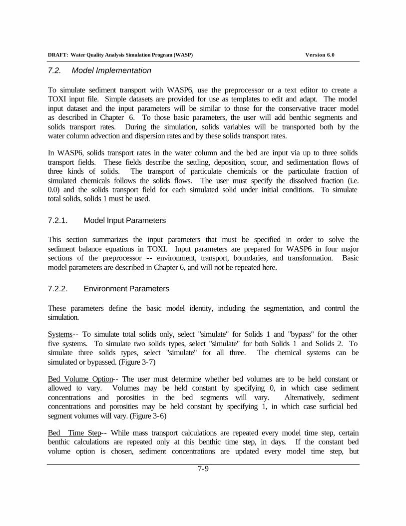
DRAFT: Water Quality Analysis Simulation Program (WASP) Version 6.0
7-9
7.2. Model Implementation
To simulate sediment transport with WASP6, use the preprocessor or a text editor to create a TOXI input file. Simple datasets are provided for use as templates to edit and adapt. The model input dataset and the input parameters will be similar to those for the conservative tracer model as described in Chapter 6. To those basic parameters, the user will add benthic segments and solids transport rates. During the simulation, solids variables will be transported both by the water column advection and dispersion rates and by these solids transport rates.
In WASP6, solids transport rates in the water column and the bed are input via up to three solids transport fields. These fields describe the settling, deposition, scour, and sedimentation flows of three kinds of solids. The transport of particulate chemicals or the particulate fraction of simulated chemicals follows the solids flows. The user must specify the dissolved fraction (i.e. 0.0) and the solids transport field for each simulated solid under initial conditions. To simulate total solids, solids 1 must be used.
7.2.1. Model Input Parameters
This section summarizes the input parameters that must be specified in order to solve the sediment balance equations in TOXI. Input parameters are prepared for WASP6 in four major sections of the preprocessor -- environment, transport, boundaries, and transformation. Basic model parameters are described in Chapter 6, and will not be repeated here.
7.2.2. Environment Parameters
These parameters define the basic model identity, including the segmentation, and control the simulation.
Systems-- To simulate total solids only, select "simulate" for Solids 1 and "bypass" for the other five systems. To simulate two solids types, select "simulate" for both Solids 1 and Solids 2. To simulate three solids types, select "simulate" for all three. The chemical systems can be simulated or bypassed. (Figure 3-7)
Bed Volume Option-- The user must determine whether bed volumes are to be held constant or allowed to vary. Volumes may be held constant by specifying 0, in which case sediment concentrations and porosities in the bed segments will vary. Alternatively, sediment concentrations and porosities may be held constant by specifying 1, in which case surficial bed segment volumes will vary. (Figure 3-6)
Bed Time Step-- While mass transport calculations are repeated every model time step, certain benthic calculations are repeated only at this benthic time step, in days. If the constant bed volume option is chosen, sediment concentrations are updated every model time step, but

DRAFT: Water Quality Analysis Simulation Program (WASP) Version 6.0
7-10
porosities are recalculated every benthic time step. If the variable bed volume is chosen, upper benthic segment volumes are updated every time step, with compaction occurring every benthic time step. (Figure 3-6)
Transport Parameters
Sediment Transport Velocities, m/sec-- Time variable settling, deposition, scour, and sedimentation velocities can be specified for each type of solid. If the units’ conversion factor is set to 1.157e-5, then these velocities are input in units of m/day. These velocities are multiplied internally by cross-sectional areas and treated as flows that carry solids and sorbed chemical between segments. Settling velocities are important components of suspended sediment transport in the water column. Scour and deposition velocities determine the transfer of solids and sorbed chemical between the water column and the sediment bed. Sedimentation velocities represent the rate at which the bed is rising in response to net deposition. (Figure 3-14)
Cross-Sectional Areas, m2-- The interfacial surface area must be specified for adjoining segments where sediment transport occurs. These surface areas are multiplied internally by sediment transport velocities to obtain sediment transport flows. ( Figure 3-14)
7.2.3. Boundary Parameters
This group of parameters includes boundary concentrations, waste loads, and initial conditions. Boundary concentrations must be specified for any segment receiving flow inputs, outputs, or exchanges. Initial conditions include not only initial concentrations, but also the density and solids transport field for each solid, and the dissolved fraction in each segment.
Boundary Concentrations, mg/L-- At each segment boundary, time variable concentrations must be specified for total solids, or for each solids type simulated. A boundary segment is characterized by water exchanges from outside the network, including tributary inflows, downstream outflows, and open water dispersive exchanges. (Figure 3-15)
Waste Loads, kg/day-- For each point source discharge, time variable sediment loads can be specified for total solids, or for each solids type simulated. These loads can represent municipal and industrial wastewater discharges, or urban and agricultural runoff. (Figure 3-16)
Solids Transport Field-- The transport field associated with total solids or each solids type must be specified under initial conditions.
Solid Density, g/cm3-- The average density of the total sediment, or the density of each solids type must be specified. This information is used to compute the porosity of benthic segments. Porosity is a function of sediment concentration and the density of each solids type. (Figure 3-7)
DRAFT: Water Quality Analysis Simulation Program (WASP) Version 6.0
7-11
Initial Concentrations, mg/L-- Concentrations of total sediment or of each solids type in each segment must be specified for the time at which the simulation begins. If the variable benthic volume option is used, the benthic sediment concentrations specified here will remain constant for the entire simulation. (Figure 3-10)
Dissolved Fraction-- The dissolved fraction of each solid in each segment should be set to 0. (Figure 3-11)
7.2.4. Transformation Parameters
This group of parameters includes spatially variable parameters, constants, and kinetic time functions for the water quality constituents being simulated. None are necessary for sediment transport.
DRAFT: Water Quality Analysis Simulation Program (WASP) Version 6.0
8-1
8. Dissolved Oxygen
Dissolved oxygen (DO) is one of the most important variables in water quality analysis. Low concentrations directly affect fish and alter a healthy ecological balance. Because DO is affected by many other water quality parameters, it is a sensitive indicator of the health of the aquatic system.
DO have been modeled for over 70 years. The basic steady-state equations were developed and used by Streeter and Phelps (1925). Subsequent development and applications have added terms to their basic equation and provided for time-variable analysis. The equations implemented here are fairly standard. As explained below, the user may implement some or all of the processes that are described with terms in these equations.
8.1. Overview of WASP6 Dissolved Oxygen
Dissolved oxygen and associated variables are simulated using the EUTRO program. Several physical-chemical processes can affect the transport and interaction among the nutrients, phytoplankton, carbonaceous material, and dissolved oxygen in the aquatic environment. Figure 8-1 presents the principal kinetic interactions for the nutrient cycles and dissolved oxygen.
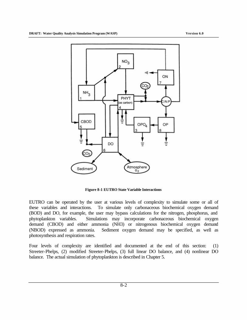
DRAFT: Water Quality Analysis Simulation Program (WASP) Version 6.0
8-2
Figure 8-1 EUTRO State Variable Interactions
EUTRO can be operated by the user at various levels of complexity to simulate some or all of these variables and interactions. To simulate only carbonaceous biochemical oxygen demand (BOD) and DO, for example, the user may bypass calculations for the nitrogen, phosphorus, and phytoplankton variables. Simulations may incorporate carbonaceous biochemical oxygen demand (CBOD) and either ammonia (NH3) or nitrogenous biochemical oxygen demand (NBOD) expressed as ammonia. Sediment oxygen demand may be specified, as well as photosynthesis and respiration rates.
Four levels of complexity are identified and documented at the end of this section: (1) Streeter-Phelps, (2) modified Streeter-Phelps, (3) full linear DO balance, and (4) nonlinear DO balance. The actual simulation of phytoplankton is described in Chapter 5.

DRAFT: Water Quality Analysis Simulation Program (WASP) Version 6.0
8-3
8.2. Dissolved Oxygen Processes
Five EUTRO state variables can participate directly in the DO balance: phytoplankton carbon, ammonia, nitrate, carbonaceous biochemical oxygen demand, and dissolved oxygen. The reduction of dissolved oxygen is a consequence of the aerobic respiratory processes in the water column and the anaerobic processes in the underlying sediments. Because both these sets of processes can contribute significantly, it is necessary to formulate their kinetics explicitly.
Figure 8-2 Oxygen balance equations
The methodology for the analysis of dissolved oxygen dynamics in natural waters, particularly in streams, rivers, and estuaries is reasonably well-developed (O'Connor and Thomann, 1972). The major and minor processes incorporated into EUTRO are discussed below. The reader should refer to the kinetic equations summarized in Figure 8-2, and the reaction parameters and coefficients in Table 8-1.
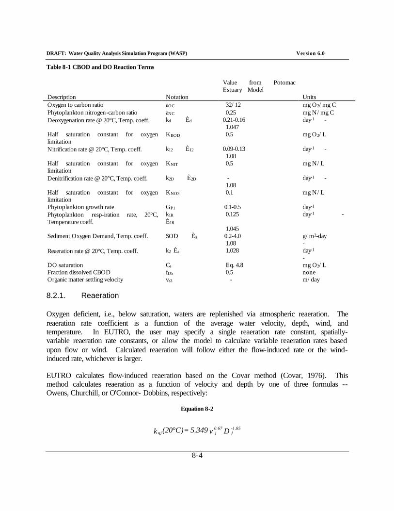
DRAFT: Water Quality Analysis Simulation Program (WASP) Version 6.0
8-4
Table 8-1 CBOD and DO Reaction Terms
Value from Potomac Estuary Model
Description Notation Units Oxygen to carbon ratio aOC 32/12 mg O2/mg C Phytoplankton nitrogen-carbon ratio aNC 0.25 mg N/mg C Deoxygenation rate @ 20°C, Temp. coeff. kd Èd 0.21-0.16
1.047 day-1 -
Half saturation constant for oxygen limitation
KBOD 0.5 mg O2/L
Nitrification rate @ 20°C, Temp. coeff. k12 È12 0.09-0.13 1.08
day-1 -
Half saturation constant for oxygen limitation
KNIT 0.5 mg N/L
Denitrification rate @ 20°C, Temp. coeff. k2D È2D - 1.08
day-1 -
Half saturation constant for oxygen limitation
KNO3 0.1 mg N/L
Phytoplankton growth rate GP1 0.1-0.5 day-1 Phytoplankton resp-iration rate, 20°C, Temperature coeff.
k1R È1R
0.125 1.045
day-1 -
Sediment Oxygen Demand, Temp. coeff. SOD Ès 0.2-4.0 1.08
g/m2-day -
Reaeration rate @ 20°C, Temp. coeff. k2 Èa 1.028 day-1 -
DO saturation Cs Eq. 4.8 mg O2/L Fraction dissolved CBOD fD5 0.5 none Organic matter settling velocity vs3 - m/day
8.2.1. Reaeration
Oxygen deficient, i.e., below saturation, waters are replenished via atmospheric reaeration. The reaeration rate coefficient is a function of the average water velocity, depth, wind, and temperature. In EUTRO, the user may specify a single reaeration rate constant, spatially-variable reaeration rate constants, or allow the model to calculate variable reaeration rates based upon flow or wind. Calculated reaeration will follow either the flow-induced rate or the wind-induced rate, whichever is larger.
EUTRO calculates flow-induced reaeration based on the Covar method (Covar, 1976). This method calculates reaeration as a function of velocity and depth by one of three formulas -- Owens, Churchill, or O'Connor- Dobbins, respectively:
Equation 8-2
D v 5.349 = C)(20k 1.85- j
0.67 j qj °
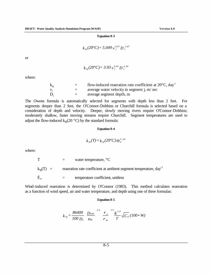
DRAFT: Water Quality Analysis Simulation Program (WASP) Version 6.0
8-5
Equation 8-3
D v 5.049 = C)(20k 1.67- j
0.97 j qj °
or
D v 3.93 = C)(20k 1.50- j
0.50 j qj °
where:
kqj = flow-induced reaeration rate coefficient at 20°C, day-1 vj = average water velocity in segment j, m/sec Dj = average segment depth, m
The Owens formula is automatically selected for segments with depth less than 2 feet. For segments deeper than 2 feet, the O'Connor-Dobbins or Churchill formula is selected based on a consideration of depth and velocity. Deeper, slowly moving rivers require O'Connor-Dobbins; moderately shallow, faster moving streams require Churchill. Segment temperatures are used to adjust the flow-induced kqj(20 °C) by the standard formula:
Equation 8-4
Θ° 20-T a qjqj C)(20k = (T)k
where:
T = water temperature, °C
kqj(T) = reaeration rate coefficient at ambient segment temperature, day-1
Èa = temperature coefficient, unitless
Wind-induced reaeration is determined by O'Connor (1983). This method calculates reaeration as a function of wind speed, air and water temperature, and depth using one of three formulas:
Equation 8-5
W) (100 C D D 100
86400 = k d
1/3
W
a
1/2
W
OW
2/3
jwj •
Γ
κρρ
ν
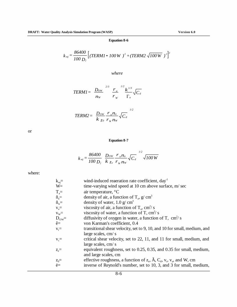
DRAFT: Water Quality Analysis Simulation Program (WASP) Version 6.0
8-6
Equation 8-6
[ ]
C
z
D = TERM2
C D = TERM1
where
)W 100 (TERM2 + )W 100 (TERM1 D 100
86400 = k
dWW
aa
0
OW
1/2
du
1/3
W
a
1/2
W
OW
2/3
1-1- 1-
jwj
Γ
•
νρνρ
κ
κρρ
ν
or
Equation 8-7
W 100 C
z
D D 100
86400 = k d
WW
aa
e
OW
1/2
jwj
νρνρ
κ
where:
kwj= wind-induced reaeration rate coefficient, day-1 W= time-varying wind speed at 10 cm above surface, m/sec Ta= air temperature, °C ña= density of air, a function of Ta, g/cm3 ñw= density of water, 1.0 g/cm3 va= viscosity of air, a function of Ta, cm2/s vW= viscosity of water, a function of T, cm2/s DOW= diffusivity of oxygen in water, a function of T, cm2/s ê= von Karman's coefficient, 0.4 vt= transitional shear velocity, set to 9, 10, and 10 for small, medium, and
large scales, cm/s vc= critical shear velocity, set to 22, 11, and 11 for small, medium, and
large scales, cm/s ze= equivalent roughness, set to 0.25, 0.35, and 0.35 for small, medium,
and large scales, cm z0= effective roughness, a function of ze, Ã, Cd, vt, va, and W, cm ë= inverse of Reynold's number, set to 10, 3, and 3 for small, medium,
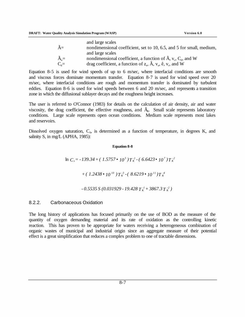
DRAFT: Water Quality Analysis Simulation Program (WASP) Version 6.0
8-7
and large scales Ã= nondimensional coefficient, set to 10, 6.5, and 5 for small, medium,
and large scales Ãu= nondimensional coefficient, a function of Ã, vc, Cd, and W Cd= drag coefficient, a function of ze, Ã, va, ê, vt, and W
Equation 8-5 is used for wind speeds of up to 6 m/sec, where interfacial conditions are smooth and viscous forces dominate momentum transfer. Equation 8-7 is used for wind speed over 20 m/sec, where interfacial conditions are rough and momentum transfer is dominated by turbulent eddies. Equation 8-6 is used for wind speeds between 6 and 20 m/sec, and represents a transition zone in which the diffusional sublayer decays and the roughness height increases.
The user is referred to O'Connor (1983) for details on the calculation of air density, air and water viscosity, the drag coefficient, the effective roughness, and Ãu. Small scale represents laboratory conditions. Large scale represents open ocean conditions. Medium scale represents most lakes and reservoirs.
Dissolved oxygen saturation, Cs, is determined as a function of temperature, in degrees K, and salinity S, in mg/L (APHA, 1985):
Equation 8-8
)T 3867.3 + T 19.428 - (0.031929 S0.5535 -
T )10 8.6219 ( - T ) 10 1.2438 ( +
T )10 6.6423 ( - T )10 1.5757 ( + 139.34- = C
2- K
1- K
4- K
11 3- K
10
2- K
7 1- K
5 s
••
••ln
8.2.2. Carbonaceous Oxidation
The long history of applications has focused primarily on the use of BOD as the measure of the quantity of oxygen demanding material and its rate of oxidation as the controlling kinetic reaction. This has proven to be appropriate for waters receiving a heterogeneous combination of organic wastes of municipal and industrial origin since an aggregate measure of their potential effect is a great simplification that reduces a complex problem to one of tractable dimensions.
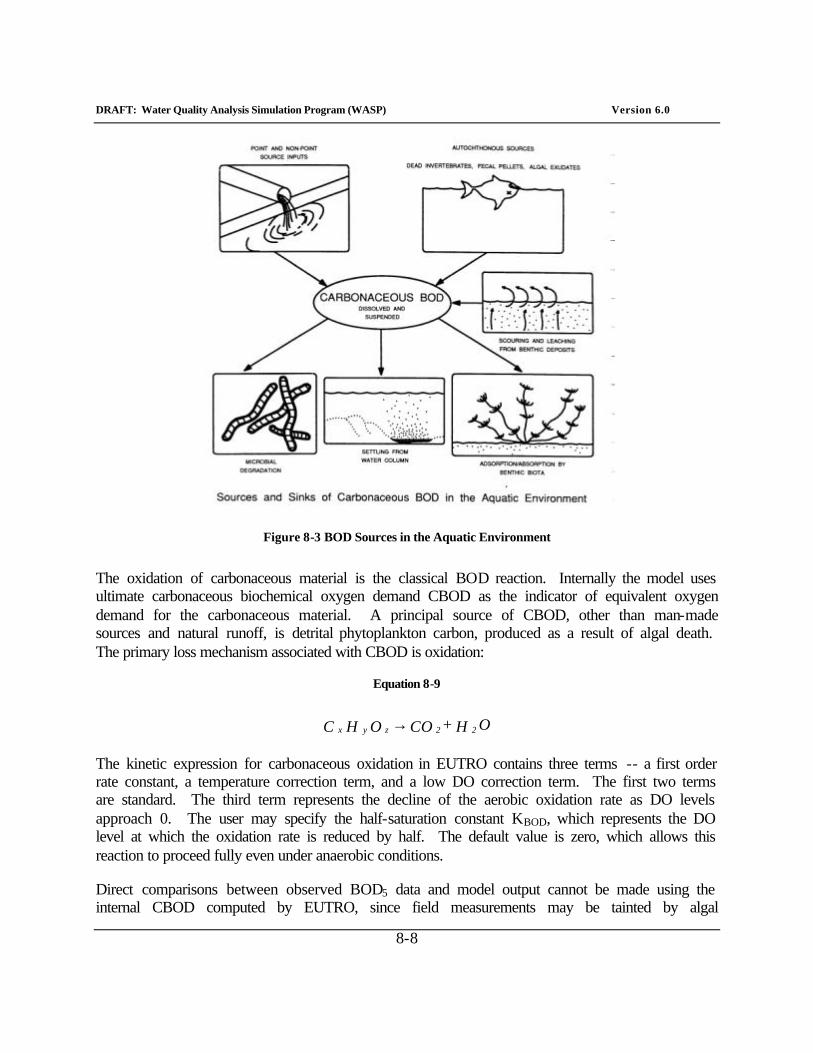
DRAFT: Water Quality Analysis Simulation Program (WASP) Version 6.0
8-8
Figure 8-3 BOD Sources in the Aquatic Environment
The oxidation of carbonaceous material is the classical BOD reaction. Internally the model uses ultimate carbonaceous biochemical oxygen demand CBOD as the indicator of equivalent oxygen demand for the carbonaceous material. A principal source of CBOD, other than man-made sources and natural runoff, is detrital phytoplankton carbon, produced as a result of algal death. The primary loss mechanism associated with CBOD is oxidation:
Equation 8-9
OH + CO O H C 2 2 z y x →
The kinetic expression for carbonaceous oxidation in EUTRO contains three terms -- a first order rate constant, a temperature correction term, and a low DO correction term. The first two terms are standard. The third term represents the decline of the aerobic oxidation rate as DO levels approach 0. The user may specify the half-saturation constant KBOD, which represents the DO level at which the oxidation rate is reduced by half. The default value is zero, which allows this reaction to proceed fully even under anaerobic conditions.
Direct comparisons between observed BOD5 data and model output cannot be made using the internal CBOD computed by EUTRO, since field measurements may be tainted by algal
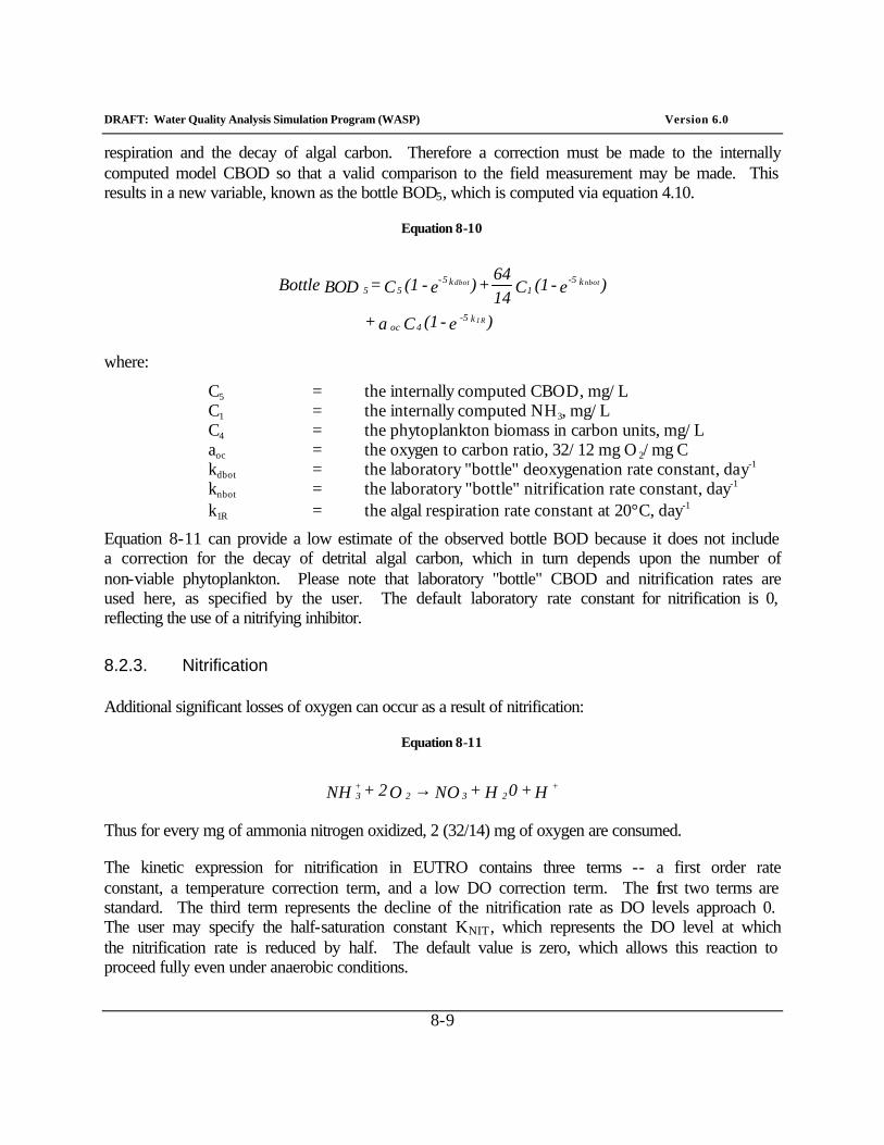
DRAFT: Water Quality Analysis Simulation Program (WASP) Version 6.0
8-9
respiration and the decay of algal carbon. Therefore a correction must be made to the internally computed model CBOD so that a valid comparison to the field measurement may be made. This results in a new variable, known as the bottle BOD5, which is computed via equation 4.10.
Equation 8-10
)e - (1 C a +
)e - (1 C 1464
+ )e - (1 C = BOD Bottle
k 5- 4oc
k 5-1
k 5-55
1R
nbotdbot
where:
C5 = the internally computed CBOD, mg/L C1 = the internally computed NH3, mg/L C4 = the phytoplankton biomass in carbon units, mg/L aoc = the oxygen to carbon ratio, 32/12 mg O2/mg C kdbot = the laboratory "bottle" deoxygenation rate constant, day-1 knbot = the laboratory "bottle" nitrification rate constant, day-1 k1R = the algal respiration rate constant at 20°C, day-1
Equation 8-11 can provide a low estimate of the observed bottle BOD because it does not include a correction for the decay of detrital algal carbon, which in turn depends upon the number of non-viable phytoplankton. Please note that laboratory "bottle" CBOD and nitrification rates are used here, as specified by the user. The default laboratory rate constant for nitrification is 0, reflecting the use of a nitrifying inhibitor.
8.2.3. Nitrification
Additional significant losses of oxygen can occur as a result of nitrification:
Equation 8-11
H + 0H + NO O 2 + NH + 2 3 2
+ 3 →
Thus for every mg of ammonia nitrogen oxidized, 2 (32/14) mg of oxygen are consumed.
The kinetic expression for nitrification in EUTRO contains three terms -- a first order rate constant, a temperature correction term, and a low DO correction term. The first two terms are standard. The third term represents the decline of the nitrification rate as DO levels approach 0. The user may specify the half-saturation constant KNIT , which represents the DO level at which the nitrification rate is reduced by half. The default value is zero, which allows this reaction to proceed fully even under anaerobic conditions.
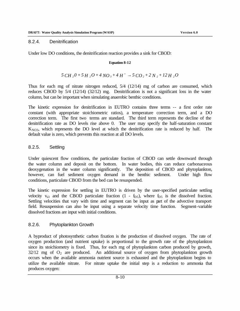
DRAFT: Water Quality Analysis Simulation Program (WASP) Version 6.0
8-10
8.2.4. Denitrification
Under low DO conditions, the denitrification reaction provides a sink for CBOD:
Equation 8-12
OH 12 + N 2 + CO 5 H 4 + NO 4 + OH 5 + 0CH 5 2 2 2 +
3 2 2 →
Thus for each mg of nitrate nitrogen reduced, 5/4 (12/14) mg of carbon are consumed, which reduces CBOD by 5/4 (12/14) (32/12) mg. Denitrification is not a significant loss in the water column, but can be important when simulating anaerobic benthic conditions.
The kinetic expression for denitrification in EUTRO contains three terms -- a first order rate constant (with appropriate stoichiometric ratios), a temperature correction term, and a DO correction term. The first two terms are standard. The third term represents the decline of the denitrification rate as DO levels rise above 0. The user may specify the half-saturation constant KNO3, which represents the DO level at which the denitrification rate is reduced by half. The default value is zero, which prevents this reaction at all DO levels.
8.2.5. Settling
Under quiescent flow conditions, the particulate fraction of CBOD can settle downward through the water column and deposit on the bottom. In water bodies, this can reduce carbonaceous deoxygenation in the water column significantly. The deposition of CBOD and phytoplankton, however, can fuel sediment oxygen demand in the benthic sediment. Under high flow conditions, particulate CBOD from the bed can be resuspended.
The kinetic expression for settling in EUTRO is driven by the user-specified particulate settling velocity vs3 and the CBOD particulate fraction (1 - fD5), where fD5 is the dissolved fraction. Settling velocities that vary with time and segment can be input as part of the advective transport field. Resuspension can also be input using a separate velocity time function. Segment-variable dissolved fractions are input with initial conditions.
8.2.6. Phytoplankton Growth
A byproduct of photosynthetic carbon fixation is the production of dissolved oxygen. The rate of oxygen production (and nutrient uptake) is proportional to the growth rate of the phytoplankton since its stoichiometry is fixed. Thus, for each mg of phytoplankton carbon produced by growth, 32/12 mg of O2 are produced. An additional source of oxygen from phytoplankton growth occurs when the available ammonia nutrient source is exhausted and the phytoplankton begins to utilize the available nitrate. For nitrate uptake the initial step is a reduction to ammonia that produces oxygen:
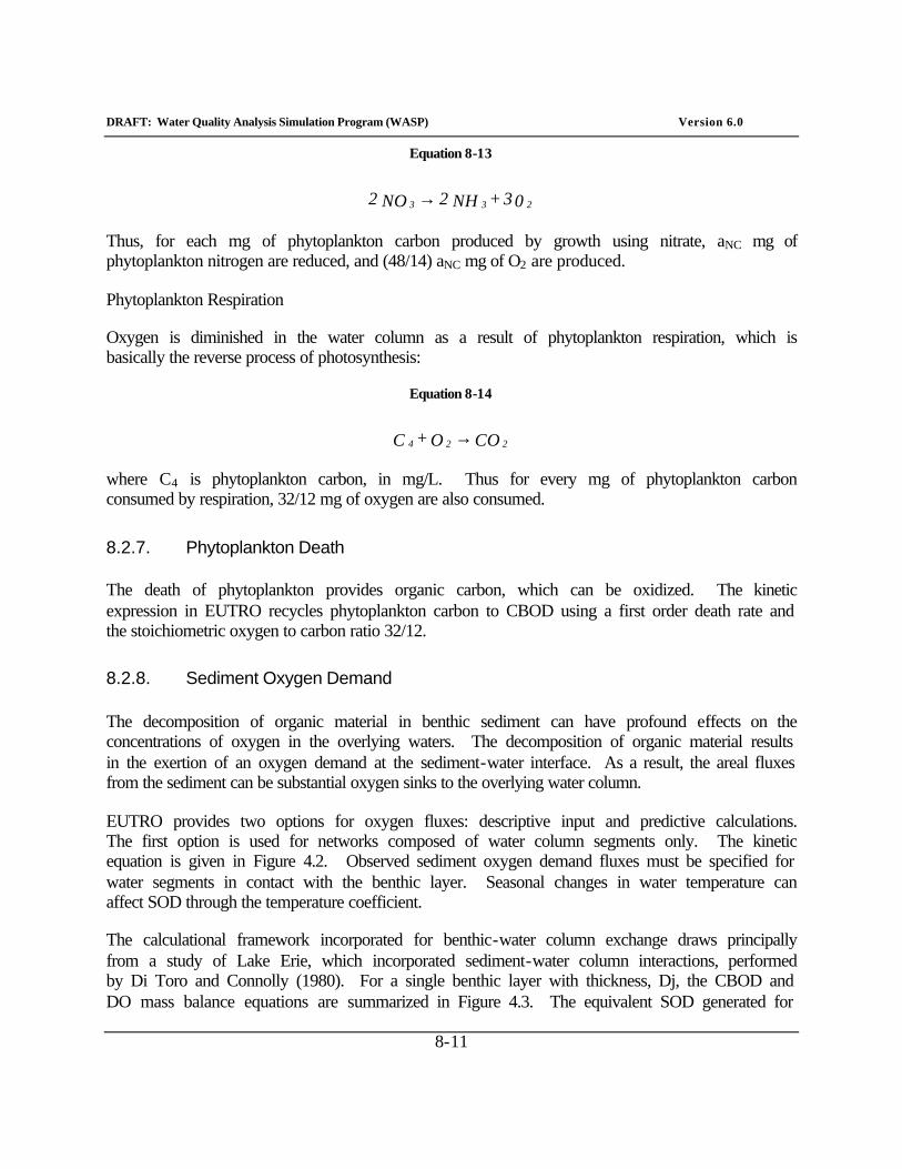
DRAFT: Water Quality Analysis Simulation Program (WASP) Version 6.0
8-11
Equation 8-13
0 3 + NH 2 NO 2 2 3 3 →
Thus, for each mg of phytoplankton carbon produced by growth using nitrate, aNC mg of phytoplankton nitrogen are reduced, and (48/14) aNC mg of O2 are produced.
Phytoplankton Respiration
Oxygen is diminished in the water column as a result of phytoplankton respiration, which is basically the reverse process of photosynthesis:
Equation 8-14
CO O + C 2 2 4 →
where C4 is phytoplankton carbon, in mg/L. Thus for every mg of phytoplankton carbon consumed by respiration, 32/12 mg of oxygen are also consumed.
8.2.7. Phytoplankton Death
The death of phytoplankton provides organic carbon, which can be oxidized. The kinetic expression in EUTRO recycles phytoplankton carbon to CBOD using a first order death rate and the stoichiometric oxygen to carbon ratio 32/12.
8.2.8. Sediment Oxygen Demand
The decomposition of organic material in benthic sediment can have profound effects on the concentrations of oxygen in the overlying waters. The decomposition of organic material results in the exertion of an oxygen demand at the sediment-water interface. As a result, the areal fluxes from the sediment can be substantial oxygen sinks to the overlying water column.
EUTRO provides two options for oxygen fluxes: descriptive input and predictive calculations. The first option is used for networks composed of water column segments only. The kinetic equation is given in Figure 4.2. Observed sediment oxygen demand fluxes must be specified for water segments in contact with the benthic layer. Seasonal changes in water temperature can affect SOD through the temperature coefficient.
The calculational framework incorporated for benthic-water column exchange draws principally from a study of Lake Erie, which incorporated sediment-water column interactions, performed by Di Toro and Connolly (1980). For a single benthic layer with thickness, Dj, the CBOD and DO mass balance equations are summarized in Figure 4.3. The equivalent SOD generated for
DRAFT: Water Quality Analysis Simulation Program (WASP) Version 6.0
8-12
the overlying water column segment is also given. Subscripts "j" and "i" refer to a benthic segment and the overlying water column segment, respectively.
WASP6 allows a more detailed parameterization of settling into the benthos that includes not only a downward settling velocity but an upward resuspension velocity as well. In this context, then, the net particulate flux to the sediment is due to the difference between the downward settling flux and the upward resuspension flux.
One of the first decisions to be made regarding the benthic layer is to determine its depth. Two factors influence this decision. The first is to adequately reflect the thickness of the active layer, the depth to which the sediment is influenced by exchange with the overlying water column. Secondly one wishes the model to reflect a reasonable time history or "memory" in the sediment layer. Too thin a layer and the benthos will "remember" or be influenced by deposition of material that would have occurred only within the last year or two of the period being analyzed; too thick a layer and the model will "average" too long a history, not reflecting substantial reductions resulting from reduced discharges from sewage treatment plants. The choice of sediment thickness is further complicated by spatially variable sedimentation rates. The benthic layer depths, together with the assigned sedimentation velocities, provide for a multi-year detention time or "memory', providing a reasonable approximation of the active layer in light of the observed pore water gradients.
The decomposition reactions that drive the component mass balance equations are the anaerobic decomposition of the phytoplankton carbon, and the anaerobic breakdown of the benthic organic carbon. Both reactions are sinks of oxygen and rapidly drive its concentration negative, indicating that the sediment is reduced rather than oxidized. The negative concentrations computed can be considered the oxygen equivalents of the reduced end products produced by the chains of redox reactions occurring in the sediment (Figure 8-4).

DRAFT: Water Quality Analysis Simulation Program (WASP) Version 6.0
8-13
Figure 8-4 Benthic layer oxygen balance equations
Because the calculated concentration of oxygen is positive in the overlying water, it is assumed that the reduced carbon species (negative oxygen equivalents) that are transported across the benthic water interface combine with the available oxygen and are oxidized to CO2 and H2O with a consequent reduction of oxygen in the overlying water column.
Table 8-2 summarize the benthic CBOD and DO reactions and parameters. Illustrative parameter values from an early Potomac Estuary modeling study are provided.
Table 8-2 Benthic Layer CBOD and DO Reaction Terms
Description Notation Value Units Organic carbon (as CBOD) decomposition rate kDS 0.0004 day-1 Temperature coefficient ÈDS 1.08 none Denitrification rate k2D day-1 Temperature coefficient È2D none Phytoplankton decomposition rate kPzD day-1
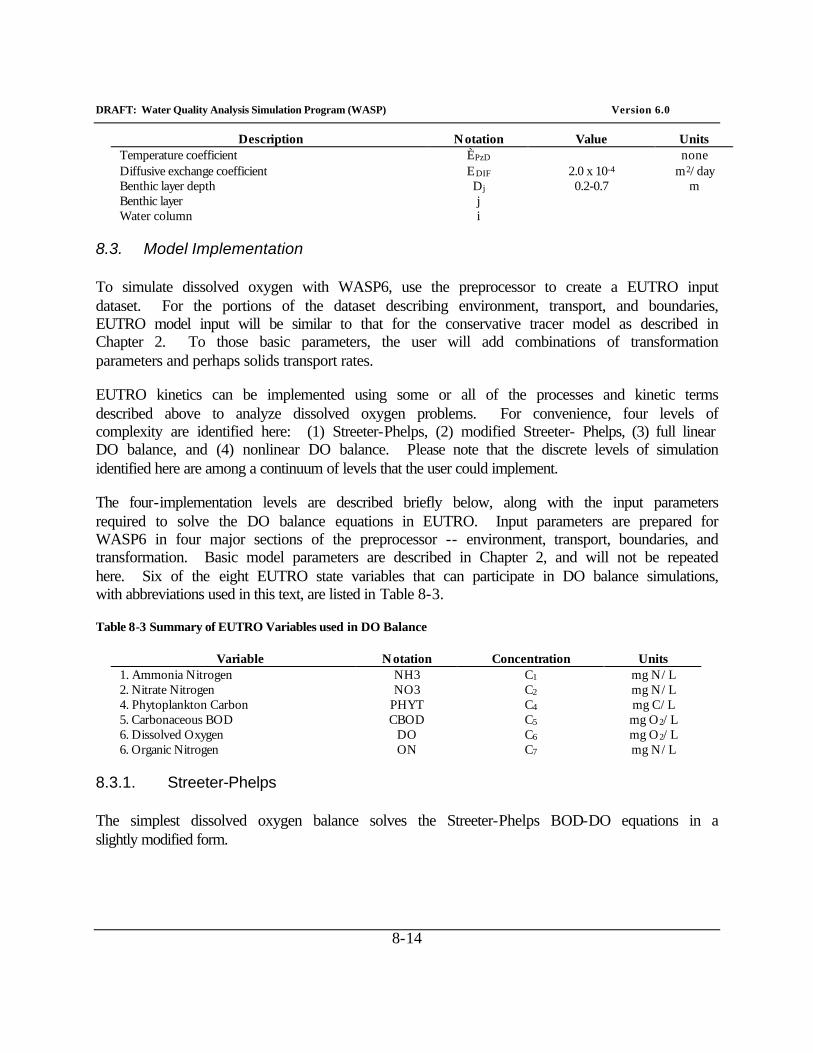
DRAFT: Water Quality Analysis Simulation Program (WASP) Version 6.0
8-14
Description Notation Value Units Temperature coefficient ÈPzD none Diffusive exchange coefficient EDIF 2.0 x 10⁻⁴ m2/day Benthic layer depth Dj 0.2-0.7 m Benthic layer j Water column i
8.3. Model Implementation
To simulate dissolved oxygen with WASP6, use the preprocessor to create a EUTRO input dataset. For the portions of the dataset describing environment, transport, and boundaries, EUTRO model input will be similar to that for the conservative tracer model as described in Chapter 2. To those basic parameters, the user will add combinations of transformation parameters and perhaps solids transport rates.
EUTRO kinetics can be implemented using some or all of the processes and kinetic terms described above to analyze dissolved oxygen problems. For convenience, four levels of complexity are identified here: (1) Streeter-Phelps, (2) modified Streeter- Phelps, (3) full linear DO balance, and (4) nonlinear DO balance. Please note that the discrete levels of simulation identified here are among a continuum of levels that the user could implement.
The four-implementation levels are described briefly below, along with the input parameters required to solve the DO balance equations in EUTRO. Input parameters are prepared for WASP6 in four major sections of the preprocessor -- environment, transport, boundaries, and transformation. Basic model parameters are described in Chapter 2, and will not be repeated here. Six of the eight EUTRO state variables that can participate in DO balance simulations, with abbreviations used in this text, are listed in Table 8-3.
Table 8-3 Summary of EUTRO Variables used in DO Balance
Variable Notation Concentration Units 1. Ammonia Nitrogen NH3 C1 mg N/L 2. Nitrate Nitrogen NO3 C2 mg N/L 4. Phytoplankton Carbon PHYT C4 mg C/L 5. Carbonaceous BOD CBOD C5 mg O2/L 6. Dissolved Oxygen DO C6 mg O2/L 6. Organic Nitrogen ON C7 mg N/L
8.3.1. Streeter-Phelps
The simplest dissolved oxygen balance solves the Streeter-Phelps BOD-DO equations in a slightly modified form.
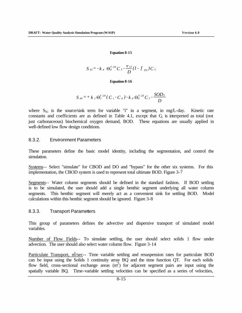
DRAFT: Water Quality Analysis Simulation Program (WASP) Version 6.0
8-15
Equation 8-15
C )f - (1 Dv - C k - = S 5 D5
s35
20-Tdd k5 Θ
Equation 8-16
DSOD - C k - )C - C( k + = S T
5 20-T
dd 6 s20-T
22 k6 ΘΘ
where Ski is the source/sink term for variable "i" in a segment, in mg/L-day. Kinetic rate constants and coefficients are as defined in Table 4.1, except that C5 is interpreted as total (not just carbonaceous) biochemical oxygen demand, BOD. These equations are usually applied in well-defined low flow design conditions.
8.3.2. Environment Parameters
These parameters define the basic model identity, including the segmentation, and control the simulation.
Systems-- Select "simulate" for CBOD and DO and "bypass" for the other six systems. For this implementation, the CBOD system is used to represent total ultimate BOD. Figure 3-7
Segments-- Water column segments should be defined in the standard fashion. If BOD settling is to be simulated, the user should add a single benthic segment underlying all water column segments. This benthic segment will merely act as a convenient sink for settling BOD. Model calculations within this benthic segment should be ignored. Figure 3-8
8.3.3. Transport Parameters
This group of parameters defines the advective and dispersive transport of simulated model variables.
Number of Flow Fields-- To simulate settling, the user should select solids 1 flow under advection. The user should also select water column flow. Figure 3-14
Particulate Transport, m3/sec-- Time variable settling and resuspension rates for particulate BOD can be input using the Solids 1 continuity array BQ and the time function QT. For each solids flow field, cross-sectional exchange areas (m2) for adjacent segment pairs are input using the spatially variable BQ. Time-variable settling velocities can be specified as a series of velocities,
DRAFT: Water Quality Analysis Simulation Program (WASP) Version 6.0
8-16
in m/sec, versus time. If the units conversion factor is set to 1.157e-5, then these velocities are input in units of m/day. These velocities are multiplied internally by cross-sectional areas and treated as flows that carry particulate organic matter out of the water column. Figure 3-14
8.3.4. Boundary Parameters
This group of parameters includes boundary concentrations, waste loads, and initial conditions. Boundary concentrations must be specified for any segment receiving flow inputs, outputs, or exchanges. Initial conditions include not only initial concentrations, but also the density and solids transport field for each solid, and the dissolved fraction in each segment.
Boundary Concentrations, mg/L-- At each segment boundary, time variable concentrations must be specified for BOD and DO. A boundary segment is characterized by water exchanges from outside the network, including tributary inflows, downstream outflows, and open water dispersive exchanges. Figure 3-15
Waste Loads, kg/day-- For each point source discharge, time variable BOD and DO loads can be specified. These loads can represent municipal and industrial wastewater discharges, or urban and agricultural runoff. (Figure 3-16)
Solids Transport Field-- The transport field associated with particulate BOD settling must be specified under initial conditions. Field 3 is recommended. (Figure 3-14)
Solid Density, g/cm3-- A value of 0 can be entered for the nominal density of BOD and DO. This information is not used in EUTRO. (Figure 3-10)
Initial Concentrations, mg/L-- Concentrations of BOD and DO in each segment must be specified for the time at which the simulation begins. Concentrations of zero for nonsimulated variables -- NH3, NO3, PO4, PHYT, ON, and OP -- will be entered by the preprocessor. ((Figure 3-10)
Dissolved Fraction-- The dissolved fraction of BOD and DO in each segment must be specified. Values for DO should be 1.0. Only the particulate fraction of BOD will be subject to settling. (Figure 3-11Figure 3-11)
8.3.5. Transformation Parameters
This group of parameters includes spatially variable parameters, constants, and kinetic time functions for the water quality constituents being simulated. Parameter values are entered for each segment. Specified values for constants apply over the entire network for the whole simulation. Kinetic time functions are composed of a series of values versus time, in days.
DRAFT: Water Quality Analysis Simulation Program (WASP) Version 6.0
8-17
Water Temperature, °C-- Segment variable water temperatures can be specified using the parameter TMPSG (parameter TMPFN and time functions TEMP(1-4) should be omitted). Temperatures will remain constant in time.
Sediment Oxygen Demand, g/m2-day-- Segment variable sediment oxygen demand fluxes can be specified using the parameter SOD1D. Values should be entered for water column segments that are in contact with the bottom of the water body.
BOD Deoxygenation Rate, day-1-- The BOD deoxygenation rate constant and temperature coefficient can be specified using constants KDC and KDT, respectively.
Reaeration Rate, day-1-- There are three options for specifying reaeration rate constants in EUTRO. In the first option, a single reaeration rate constant can be specified using constant K2. An internal temperature coefficient of 1.028 is used with this option.
If K2 is not entered (or is set to 0), the second option is attempted by EUTRO. In this option, variable reaeration rate constants can be input using parameter REARSG and time function REAR. The product of spatially variable REARSG and time-variable REAR gives the segment and time specific reaeration rate constants used by EUTRO. These reaeration values are not modified by a temperature function.
The third option is invoked if neither K2 nor REARSG is entered. In this option, reaeration rates will be calculated from water velocity, depth, wind velocity, and water and air temperature. The actual reaeration rate used by EUTRO will be either the flow or wind-induced value whichever is largest.
For rivers, segment water velocities and depths are calculated as a function of flow using the hydraulic coefficients entered under the topic "environment". For lakes and estuaries, ambient velocities in m/sec can be input using parameter VELFN and time functions VEL(1-4). The parameter VELFN indicates which velocity function will be used by the model for each segment. Values of 1.0, 2.0, 3.0, or 4.0 will call time functions VELN(1), VELN(2), VELN(3), and VELN(4), respectively. Water velocities should then be entered via these time functions as a series of velocity versus time values.
For open bodies of water, wind-driven reaeration can be significant. The user should input ambient wind speed, in m/sec, and air temperature, in °C, using time functions WIND and AIRTMP. The default values for wind speed and air temperature are 0.6 m/sec and 15 C. The scale of the water body should be input using constant WTYPE. Values of 1.0, 2.0, and 3.0 indicate laboratory scale, lake and reservoir scale, and open ocean scale, respectively. The default value is 2.
For estuaries, where salinity affects DO saturation significantly, salinity values in g/L can be input using parameter SAL and time function SALFN. The product of spatially-variable SAL
DRAFT: Water Quality Analysis Simulation Program (WASP) Version 6.0
8-18
and time-variable SALFN gives the segment and time specific salinity values used by EUTRO. Average segment salinity values can be input to SAL, while relative variations in time, if significant, can be input to SALFN.
For northern climates, where ice cover can affect reaeration during winter months, the user may input the fraction of water surface available for reaeration using time function XICECVR. A value of 1.0 indicates that the entire surface area is available for reaeration. The time variable value of XICECVR will be multiplied by the reaeration rate constants for options 1 and 3. For option 2, it is assumed that ice cover is built into the time function REAR.
WTYPE and K2 are identified in EUTRO as constants.. VELFN, SAL, and REARSG are identified in EUTRO as parameters. WIND, VELN(1-4), SALFN, AIRTMP, XICECVR, and REAR are identified in EUTRO as time functions.
8.4. Modified Streeter-Phelps
The modified Streeter-Phelps equations divide biochemical oxygen demand into carbonaceous and nitrogenous fractions, and allow time-variable temperatures to be specified. This allows for more realistic calibration to observed data. Waste load allocations, however, are usually projected for design low-flow conditions (Figure 8-5).
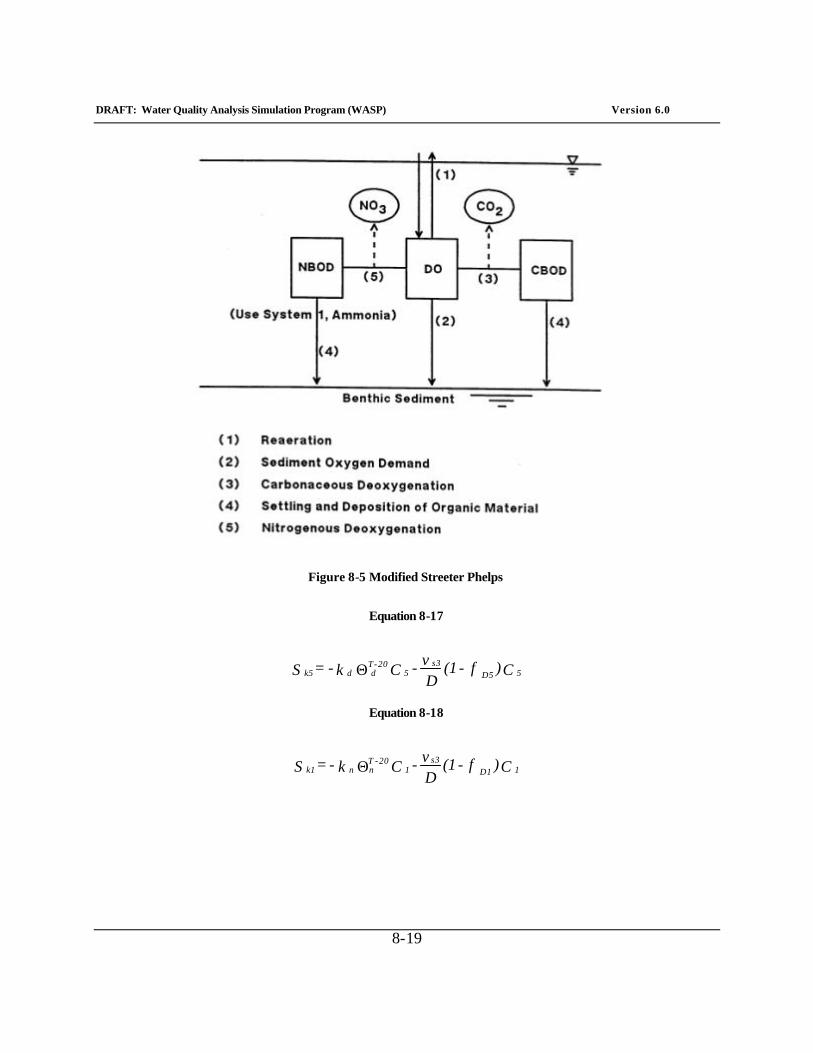
DRAFT: Water Quality Analysis Simulation Program (WASP) Version 6.0
8-19
Figure 8-5 Modified Streeter Phelps
Equation 8-17
C )f - (1 Dv - C k - = S 5 D5
s35
20-Td d k5 Θ
Equation 8-18
C )f - (1Dv - C k - = S 1 D1
s31
20-Tnn k1 Θ
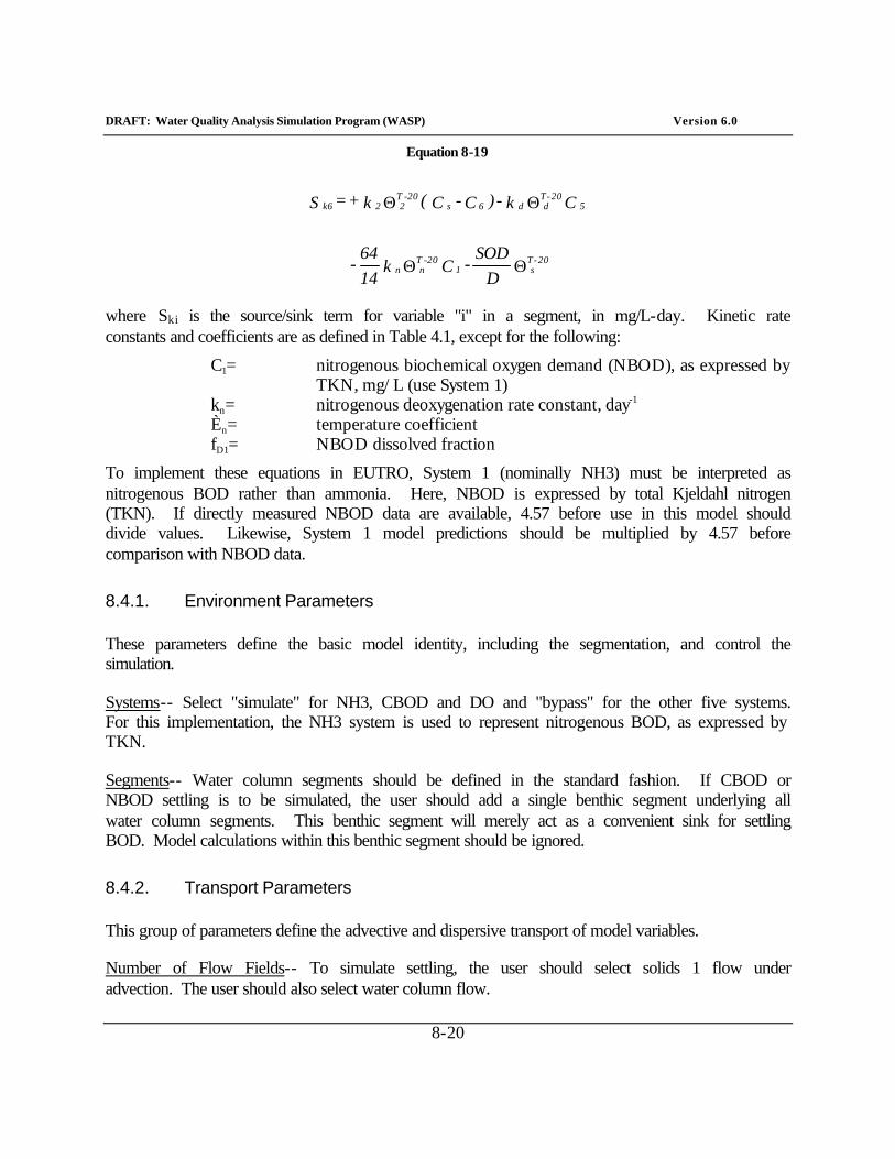
DRAFT: Water Quality Analysis Simulation Program (WASP) Version 6.0
8-20
Equation 8-19
ΘΘ
ΘΘ
20-T s1
20-Tn n
5 20-T
d d 6 s20-T
2 2 k6
D
SOD - C k
1464 -
C k - )C - C ( k + = S
where Ski is the source/sink term for variable "i" in a segment, in mg/L-day. Kinetic rate constants and coefficients are as defined in Table 4.1, except for the following:
C1= nitrogenous biochemical oxygen demand (NBOD), as expressed by TKN, mg/L (use System 1)
kn= nitrogenous deoxygenation rate constant, day-1 Èn= temperature coefficient fD1= NBOD dissolved fraction
To implement these equations in EUTRO, System 1 (nominally NH3) must be interpreted as nitrogenous BOD rather than ammonia. Here, NBOD is expressed by total Kjeldahl nitrogen (TKN). If directly measured NBOD data are available, 4.57 before use in this model should divide values. Likewise, System 1 model predictions should be multiplied by 4.57 before comparison with NBOD data.
8.4.1. Environment Parameters
These parameters define the basic model identity, including the segmentation, and control the simulation.
Systems-- Select "simulate" for NH3, CBOD and DO and "bypass" for the other five systems. For this implementation, the NH3 system is used to represent nitrogenous BOD, as expressed by TKN.
Segments-- Water column segments should be defined in the standard fashion. If CBOD or NBOD settling is to be simulated, the user should add a single benthic segment underlying all water column segments. This benthic segment will merely act as a convenient sink for settling BOD. Model calculations within this benthic segment should be ignored.
8.4.2. Transport Parameters
This group of parameters define the advective and dispersive transport of model variables.
Number of Flow Fields-- To simulate settling, the user should select solids 1 flow under advection. The user should also select water column flow.
DRAFT: Water Quality Analysis Simulation Program (WASP) Version 6.0
8-21
Particulate Transport, m3/sec-- Time variable settling and resuspension rates for particulate CBOD and NBOD can be input using the Solids 1 continuity array BQ and the time function QT. For each solids flow field, cross-sectional exchange areas (m2) for adjacent segment pairs are input using the spatially-variable BQ. Time-variable settling velocities can be specified as a series of velocities, in m/sec, versus time. If the units conversion factor is set to 1.157e-5, then these velocities are input in units of m/day. These velocities are multiplied internally by cross-sectional areas and treated as flows that carry particulate organic matter out of the water column.
8.4.3. Boundary Parameters
This group of parameters includes boundary concentrations, waste loads, and initial conditions. Boundary concentrations must be specified for any segment receiving flow inputs, outputs, or exchanges. Initial conditions include not only initial concentrations, but also the density and solids transport field for each solid, and the dissolved fraction in each segment.
Boundary Concentrations, mg/L-- At each segment boundary, time variable concentrations must be specified for CBOD, NBOD, and DO. The NH3 system is used to represent NBOD, which is expressed as TKN. A boundary segment is characterized by water exchanges from outside the network, including tributary inflows, downstream outflows, and open water dispersive exchanges.
Waste Loads, kg/day-- For each point source discharge, time variable CBOD, NBOD, and DO loads can be specified. These loads can represent municipal and industrial wastewater discharges, or urban and agricultural runoff. The NH3 system is used to represent NBOD, which is expressed as TKN.
Solids Transport Field-- The transport field associated with particulate CBOD and NBOD settling must be specified under initial conditions. Field 3 is recommended for both.
Solid Density, g/cm3-- A value of 0 can be entered for the nominal density of CBOD, NBOD, and DO. This information is not used in EUTRO.
Initial Concentrations, mg/L-- Concentrations of CBOD, NBOD, and DO in each segment must be specified for the time at which the simulation begins. The NH3 system is used to represent NBOD, which is expressed as TKN. Concentrations of zero for non-simulated variables -- NO3, PO4, PHYT, ON, and OP -- will be entered by the preprocessor.
Dissolved Fraction-- The dissolved fraction of CBOD, NBOD, and DO in each segment must be specified. Values for DO should be 1.0. Only the particulate fraction of CBOD and NBOD will be subject to settling.
DRAFT: Water Quality Analysis Simulation Program (WASP) Version 6.0
8-22
8.4.4. Transformation Parameters
This group of parameters includes spatially variable parameters, constants, and kinetic time functions for the water quality constituents being simulated. Parameter values are entered for each segment. Specified values for constants apply over the entire network for the whole simulation. Kinetic time functions are composed of a series of values versus time, in days.
Water Temperature, °C-- Time and segment variable water temperatures can be specified using the parameters TMPSG and TMPFN, and the time functions TEMP(1-4). If temperatures are to remain constant in time, then the user should enter segment temperatures using the parameter TMPSG. TMPFN and TEMP(1-4) should be omitted.
If the user wants to enter time-variable temperatures, then values for the parameter TMPSG should be set to 1.0. The parameter TMPFN indicates which temperature function will be used by the model for each segment. Values of 1.0, 2.0, 3.0, or 4.0 will call time functions TEMP(1), TEMP(2), TEMP(3), and TEMP(4), respectively. Water temperatures should then be entered via these time functions as a series of temperature versus time values. The product of TMPSG and the selected TEMP function will give the segment and time specific water temperatures used by EUTRO.
TMPSG and TMPFN are identified in EUTRO as parameters 3 and 4, respectively. TEMP(1-4) are identified in EUTRO as time functions 1-4.
Sediment Oxygen Demand, g/m2-day-- Segment variable sediment oxygen demand fluxes and temperature coefficients can be specified using the parameters SOD1D and SODTA, respectively. Values should be entered for water column segments that are in contact with the bottom of the water body. If temperatures remain constant in time, then SODTA can be omitted.
CBOD Deoxygenation Rate, day-1-- The CBOD deoxygenation rate constant and temperature coefficient can be specified using constants KDC and KDT, respectively.
NBOD Deoxygenation Rate, day-1-- The NBOD deoxygenation rate constant and temperature coefficient can be specified using constants K12C and K12T, respectively.
Reaeration Rate, day-1-- There are three basic options for specifying reaeration -- a single rate constant, segment and time variable rate constants, and flow and wind calculated rate constants. These options are described in the Streeter-Phelps section.
8.5. Full Linear DO Balance
The full DO balance equations divide the NBOD process into mineralization and nitrification, and add the effects of photosynthesis and respiration from given phytoplankton levels (Figure 8-6):

DRAFT: Water Quality Analysis Simulation Program (WASP) Version 6.0
8-23
Figure 8-6 Full Linear DO
Equation 8-20
C )f - (1 Dv - C k - = s 7 D7
s37
20-T71 71 k7 Θ
Equation 8-21
C k - C k + = S 1 20-T
12 12 7 20-T
71 71 k1 ΘΘ
Equation 8-22
C k + = S 1 20-T
12 12 k2 Θ
Equation 8-23
C )f - (1 Dv - C k - = S 5 D5
s35
20-Td d k5 Θ
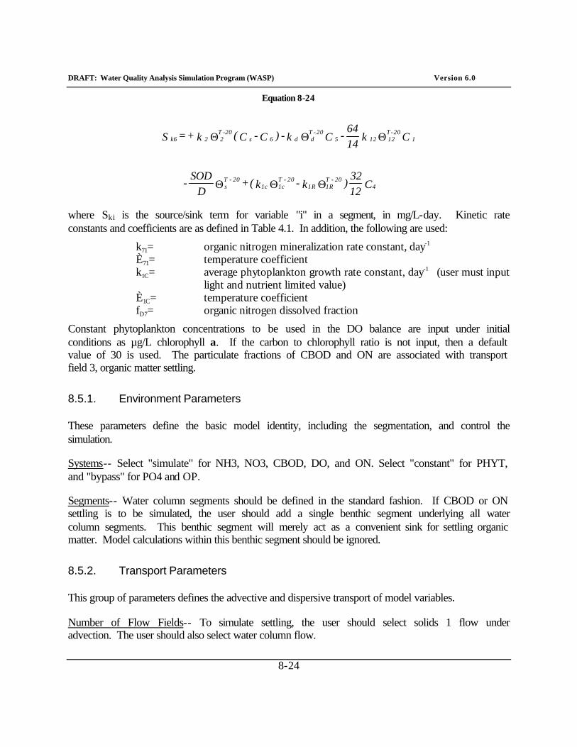
DRAFT: Water Quality Analysis Simulation Program (WASP) Version 6.0
8-24
Equation 8-24
C 1232
) k - k( + D
SOD-
C k 1464 - C k - )C - C( k + = S
420 - T
1R1R20 - T
1c1c20 - T
s
1 20-T
12 12 5 20-T
d d 6 s20-T
2 2 k6
ΘΘΘ
ΘΘΘ
where Ski is the source/sink term for variable "i" in a segment, in mg/L-day. Kinetic rate constants and coefficients are as defined in Table 4.1. In addition, the following are used:
k71= organic nitrogen mineralization rate constant, day-1 È71= temperature coefficient k1C= average phytoplankton growth rate constant, day-1 (user must input
light and nutrient limited value) È1C= temperature coefficient fD7= organic nitrogen dissolved fraction
Constant phytoplankton concentrations to be used in the DO balance are input under initial conditions as µg/L chlorophyll a. If the carbon to chlorophyll ratio is not input, then a default value of 30 is used. The particulate fractions of CBOD and ON are associated with transport field 3, organic matter settling.
8.5.1. Environment Parameters
These parameters define the basic model identity, including the segmentation, and control the simulation.
Systems-- Select "simulate" for NH3, NO3, CBOD, DO, and ON. Select "constant" for PHYT, and "bypass" for PO4 and OP.
Segments-- Water column segments should be defined in the standard fashion. If CBOD or ON settling is to be simulated, the user should add a single benthic segment underlying all water column segments. This benthic segment will merely act as a convenient sink for settling organic matter. Model calculations within this benthic segment should be ignored.
8.5.2. Transport Parameters
This group of parameters defines the advective and dispersive transport of model variables.
Number of Flow Fields-- To simulate settling, the user should select solids 1 flow under advection. The user should also select water column flow.
DRAFT: Water Quality Analysis Simulation Program (WASP) Version 6.0
8-25
Particulate Transport, m3/sec-- Time variable settling and resuspension rates for particulate CBOD and ON can be input using the Solids 1 continuity array BQ and the time function QT. For each solids flow field, cross-sectional exchange areas (m2) for adjacent segment pairs are input using the spatially-variable BQ. Time-variable settling velocities can be specified as a series of velocities, in m/sec, versus time. If the units conversion factor is set to 1.157e-5, then these velocities are input in units of m/day. These velocities are multiplied internally by cross-sectional areas and treated as flows that carry particulate organic matter out of the water column.
8.5.3. Boundary Parameters
This group of parameters includes boundary concentrations, waste loads, and initial conditions. Boundary concentrations must be specified for any segment receiving flow inputs, outputs, or exchanges. Initial conditions include not only initial concentrations, but also the density and solids transport field for each solid, and the dissolved fraction in each segment.
Boundary Concentrations, mg/L-- At each segment boundary, time variable concentrations must be specified for NH3, NO3, ON, CBOD, and DO. A boundary segment is characterized by water exchanges from outside the network, including tributary inflows, downstream outflows, and open water dispersive exchanges.
Waste Loads, kg/day-- For each point source discharge, time variable NH3, NO3, ON, CBOD, and DO loads can be specified. These loads can represent municipal and industrial wastewater discharges, or urban and agricultural runoff.
Solids Transport Field-- The transport field associated with particulate CBOD and ON settling must be specified under initial conditions. Field 3 is recommended for both.
Solid Density, g/cm3-- A value of 0 can be entered for the nominal density of NH3, NO3, ON, CBOD, and DO. This information is not used in EUTRO.
Initial Concentrations, mg/L-- Concentrations of NH3, NO3, ON, CBOD, and DO in each segment must be specified for the time at which the simulation begins. Average concentrations of PHYT, expressed as µg/L chlorophyll a, must be specified as well. These are converted to mg/L phytoplankton carbon in EUTRO using a default carbon to chlorophyll ration of 30. Phytoplankton concentrations will remain constant throughout the simulation and affect DO through photosynthesis and respiration. Concentrations of zero for non-simulated variables -- PO4 and OP -- will be entered by the preprocessor.
Dissolved Fraction-- The dissolved fraction of NH3, NO3, ON, CBOD, and DO in each segment must be specified. Values for DO should be 1.0. Only the particulate fraction of CBOD and ON will be subject to settling.

DRAFT: Water Quality Analysis Simulation Program (WASP) Version 6.0
8-26
8.5.4. Transformation Parameters
This group of parameters includes spatially variable parameters, constants, and kinetic time functions for the water quality constituents being simulated. Parameter values are entered for each segment. Specified values for constants apply over the entire network for the whole simulation. Kinetic time functions are composed of a series of values versus time, in days.
Water Temperature, °C-- Time and segment variable water temperatures can be specified using the parameters TMPSG and TMPFN, and the time functions TEMP(1-4), as described in the modified Streeter-Phelps section.
Sediment Oxygen Demand, g/m2-day-- Segment variable sediment oxygen demand fluxes and temperature coefficients can be specified using the parameters SOD1D and SODTA, respectively. Values should be entered for water column segments that are in contact with the bottom of the water body.
Nitrogen Mineralization Rate, day-1-- The mineralization rate constant and temperature coefficient for dissolved organic nitrogen can be specified using constants K71C and K71T, respectively.
Nitrification Rate, day-1-- The nitrification rate constant and temperature coefficient for dissolved ammonia nitrogen can be specified using constants K12C and K12T, respectively.
CBOD Deoxygenation Rate, day-1-- The CBOD deoxygenation rate constant and temperature coefficient can be specified using constants KDC and KDT, respectively.
Reaeration Rate, day-1-- There are three basic options for specifying reaeration -- a single rate constant, segment and time variable rate constants, and flow and wind calculated rate constants. These options are described in the Streeter-Phelps section.
Photosynthesis Rate, day-1-- The average phytoplankton growth rate constant and temperature coefficient can be input using constants K1C and K1T, respectively. For DO balance simulations where phytoplankton dynamics are bypassed, the growth rate constant must reflect average light and nutrient limitations in the water body.
Respiration Rate, day-1-- The average phytoplankton respiration rate constant and temperature coefficient can be input-using constants K1RC and K1RT, respectively.
8.6. Nonlinear DO Balance
The nonlinear DO balance equations add feedback from DO concentrations to terms in the linear DO balance equations presented above. This feedback can become important in inhibiting
DRAFT: Water Quality Analysis Simulation Program (WASP) Version 6.0
8-27
nitrification and carbonaceous oxidation and in promoting denitrification where low DO concentrations occur.
For this level of analysis, the linear DO balance equations presented above are supplemented with nonlinear terms for carbonaceous oxidation, nitrification, and denitrification. These terms are presented in Table 8-1. The environment, transport, and boundary parameters required to implement the nonlinear DO balance are the same as those in the linear DO balance presented above. The user should supplement the transformation parameters presented above with the following.
Nitrification Rate, day-1-- The nitrification rate constant and temperature coefficient for dissolved ammonia nitrogen can be specified using constants K12C and K12T, respectively. The half-saturation constant for oxygen limitation of nitrification can be specified using constant KNIT. The default value for KNIT is 0.0, indicating no oxygen limitation.
Denitrification Rate, day-1-- The denitrification rate constant and temperature coefficient for dissolved nitrate nitrogen can be specified using constants K20C and K20T, respectively. The half-saturation constant for oxygen limitation of denitrification can be specified using constant KNO3. The default value for KNO3 is 0.0, indicating no denitrification at oxygen concentrations above 0.0.
CBOD Deoxygenation Rate, day-1-- The CBOD deoxygenation rate constant and temperature coefficient can be specified using constants KDC and KDT, respectively. The half-saturation constant for oxygen limitation of carbonaceous deoxygenation can be specified using constant KBOD. The default value for KBOD is 0.0, indicating no oxygen limitation.
DRAFT: Water Quality Analysis Simulation Program (WASP) Version 6.0
9-1
9. Eutrophication
Nutrient enrichment and eutrophication are continuing concerns in many water bodies. High concentrations of nitrogen and phosphorus can lead to periodic phytoplankton blooms and an alteration of the natural trophic balance. Dissolved oxygen levels can fluctuate widely, and low DO concentrations in bottom waters can result.
Eutrophication has been modeled for approximately 30 years. The equations implemented here were derived from the Potomac Eutrophication Model, PEM (Thomann and Fitzpatrick, 1982), and are fairly standard. Sections of this text are modified from the PEM documentation report.
9.1. Overview of WASP6 Eutrophication
The nutrient enrichment, eutrophication, and DO depletion processes are simulated using the EUTRO program. Several physical-chemical processes can affect the transport and interaction among the nutrients, phytoplankton, carbonaceous material, and dissolved oxygen in the aquatic environment. Figure 9-1 presents the principal kinetic interactions for the nutrient cycles and dissolved oxygen.
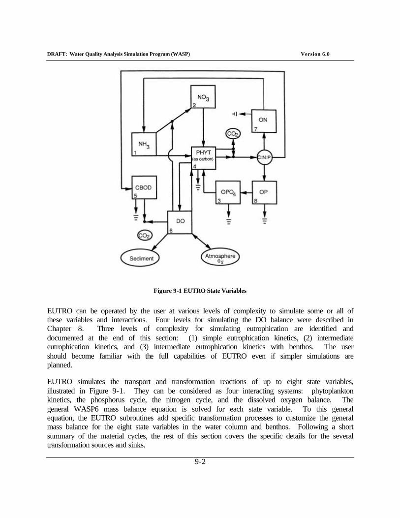
DRAFT: Water Quality Analysis Simulation Program (WASP) Version 6.0
9-2
Figure 9-1 EUTRO State Variables
EUTRO can be operated by the user at various levels of complexity to simulate some or all of these variables and interactions. Four levels for simulating the DO balance were described in Chapter 8. Three levels of complexity for simulating eutrophication are identified and documented at the end of this section: (1) simple eutrophication kinetics, (2) intermediate eutrophication kinetics, and (3) intermediate eutrophication kinetics with benthos. The user should become familiar with the full capabilities of EUTRO even if simpler simulations are planned.
EUTRO simulates the transport and transformation reactions of up to eight state variables, illustrated in Figure 9-1. They can be considered as four interacting systems: phytoplankton kinetics, the phosphorus cycle, the nitrogen cycle, and the dissolved oxygen balance. The general WASP6 mass balance equation is solved for each state variable. To this general equation, the EUTRO subroutines add specific transformation processes to customize the general mass balance for the eight state variables in the water column and benthos. Following a short summary of the material cycles, the rest of this section covers the specific details for the several transformation sources and sinks.
DRAFT: Water Quality Analysis Simulation Program (WASP) Version 6.0
9-3
9.1.1. Phosphorus Cycle
Dissolved or available inorganic phosphorus (DIP) interacts with particulate inorganic phosphorus via a sorption-desorption mechanism. DIP is taken up by phytoplankton for growth, and is incorporated into phytoplankton biomass. Phosphorus is returned from the phytoplankton biomass pool to dissolved and particulate organic phosphorus and to dissolved inorganic phosphorus through endogenous respiration and nonpredatory mortality. Organic phosphorus is converted to dissolved inorganic phosphorus at a temperature-dependent mineralization rate.
9.1.2. Nitrogen Cycle
The kinetics of the nitrogen species are fundamentally the same as the phosphorus system. Ammonia and nitrate are taken up by phytoplankton for growth, and incorporated into phytoplankton biomass. The rate at which each is taken up is a function of its concentration relative to the total inorganic nitrogen (ammonia plus nitrate) available. Nitrogen is returned from the phytoplankton biomass pool to dissolved and particulate organic nitrogen and to ammonia through endogenous respiration and nonpredatory mortality. Organic nitrogen is converted to ammonia at a temperature dependent mineralization rate, and ammonia is then converted to nitrate at a temperature- and oxygen-dependent nitrification rate. Nitrate may be converted to nitrogen gas in the absence of oxygen at a temperature- and oxygen-dependent denitrification rate.
9.1.3. Dissolved Oxygen
Dissolved oxygen is coupled to the other state variables. The sources of oxygen considered are reaeration and evolution by phytoplankton during growth. The sinks of oxygen are algal respiration, oxidation of detrital carbon and carbonaceous material from waste effluents and nonpoint discharges, and nitrification. These processes are discussed in Chapter 8.
9.1.4. Phytoplankton Kinetics
Phytoplankton kinetics assumes a central role in eutrophication, affecting all other systems. An overview of this system is given in Figure 5.2.
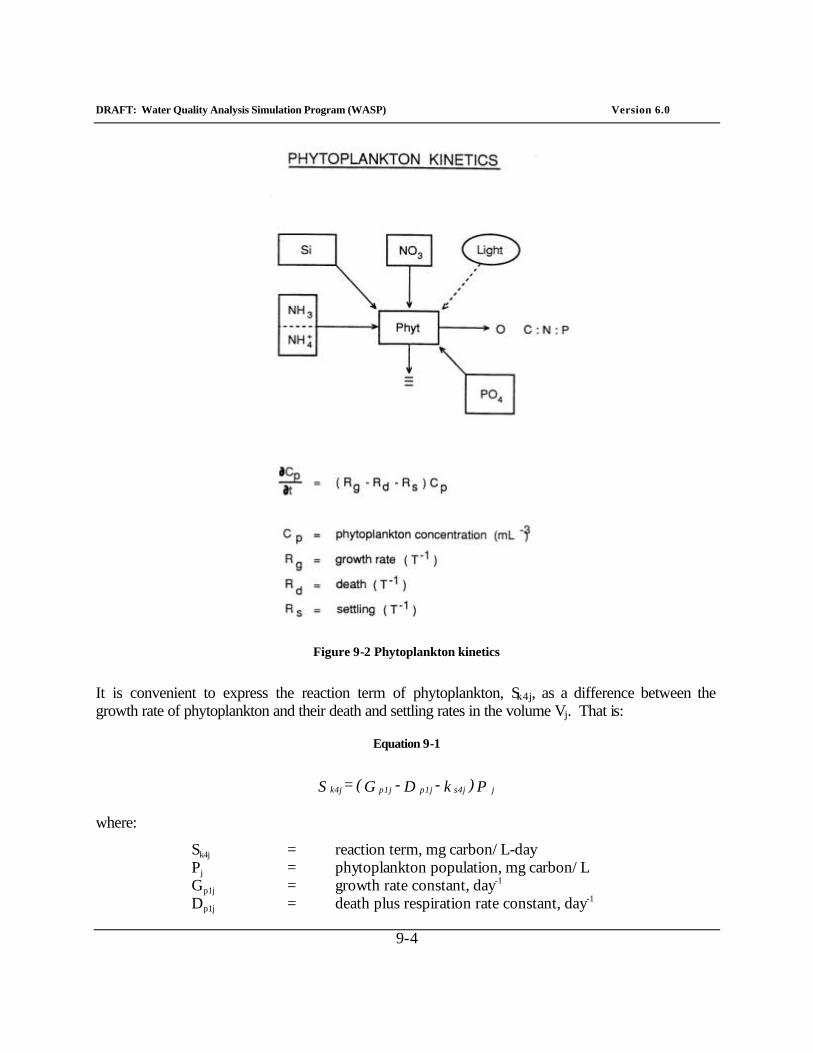
DRAFT: Water Quality Analysis Simulation Program (WASP) Version 6.0
9-4
Figure 9-2 Phytoplankton kinetics
It is convenient to express the reaction term of phytoplankton, Sk4j, as a difference between the growth rate of phytoplankton and their death and settling rates in the volume Vj. That is:
Equation 9-1
P )k - D - G( = S j s4jp1j p1j k4j
where:
Sk4j = reaction term, mg carbon/L-day Pj = phytoplankton population, mg carbon/L Gp1j = growth rate constant, day-1 Dp1j = death plus respiration rate constant, day-1

DRAFT: Water Quality Analysis Simulation Program (WASP) Version 6.0
9-5
ks4j = settling rate constant, day-1 j = segment number, unitless
The subscript 1 identifies the quantities as referring to phytoplankton type 1, (only one type is considered in this particular model); the subscript j refers to the volume element being considered. The balance between the magnitude of the growth rate and death rate (together with the transport, settling, and mixing) determines the rate at which phytoplankton mass is created in the volume element Vj. In subsequent text and in figures, subscripts i and j will be omitted unless needed for clarity.
9.1.5. Phytoplankton Growth
The growth rate of a population of phytoplankton in a natural environment is a complicated function of the species of phytoplankton present and their differing reactions to solar radiation, temperature, and the balance between nutrient availability and phytoplankton requirements. The available information is not sufficiently detailed to specify the growth kinetics for individual algal species in a natural environment. Rather than considering the problem of different species and their associated environmental and nutrient requirements, this model characterizes the population as a whole by the total biomass of the phytoplankton present.
A simple measure of total biomass that is characteristic of all phytoplankton, chlorophyll a, is used as the aggregated variable. The principal advantages are that the measurement is direct; it integrates cell types and ages, and it accounts for cell viability. The principal disadvantage is that it is a community measurement with no differentiation of functional groups (e.g., diatoms, blue-greens); also, it is not necessarily a good measurement of standing crop in dry weight or carbon units because the chlorophyll-to-dry-weight and carbon ratios are variable and non-active chlorophyll (phaeopigments) must be measured to determine viable chlorophyll concentrations.
As can be seen from the above discussion, no simple aggregate measurement is entirely satisfactory. From a practical point of view, the availability of extensive chlorophyll data essentially dictates its use as the aggregate measure of the phytoplankton population or biomass for calibration and verification purposes. For internal computational purposes, however, EUTRO uses phytoplankton carbon as a measure of algal biomass. Using either a fixed or variable carbon to chlorophyll mechanism (discussed subsequently), phytoplankton chlorophyll a may be computed and used as the calibration and verification variable to be compared against observed chlorophyll a field data.
With a choice of biomass units established, a growth rate that expresses the rate of production of biomass as a function of the important environmental variables (temperature, light, and nutrients) may be developed. The specific growth rate, GPlj, in segment j is related to k1c, the maximum 20°C growth rate at optimum light and nutrients, via the following equation.
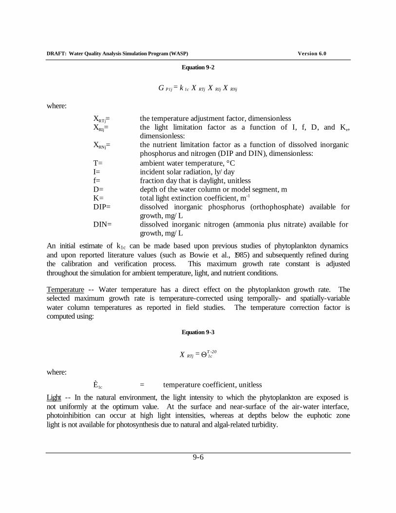
DRAFT: Water Quality Analysis Simulation Program (WASP) Version 6.0
9-6
Equation 9-2
X X X k = G RNj RIj RTj 1c P1j
where:
XRTj= the temperature adjustment factor, dimensionless XRIj= the light limitation factor as a function of I, f, D, and Ke,
dimensionless: XRNj= the nutrient limitation factor as a function of dissolved inorganic
phosphorus and nitrogen (DIP and DIN), dimensionless: T= ambient water temperature, °C I= incident solar radiation, ly/day f= fraction day that is daylight, unitless D= depth of the water column or model segment, m K= total light extinction coefficient, m-1 DIP= dissolved inorganic phosphorus (orthophosphate) available for
growth, mg/L DIN= dissolved inorganic nitrogen (ammonia plus nitrate) available for
growth, mg/L
An initial estimate of k1c can be made based upon previous studies of phytoplankton dynamics and upon reported literature values (such as Bowie et al., 1985) and subsequently refined during the calibration and verification process. This maximum growth rate constant is adjusted throughout the simulation for ambient temperature, light, and nutrient conditions.
Temperature -- Water temperature has a direct effect on the phytoplankton growth rate. The selected maximum growth rate is temperature-corrected using temporally- and spatially-variable water column temperatures as reported in field studies. The temperature correction factor is computed using:
Equation 9-3
Θ 20-T1c RTj = X
where:
È1c = temperature coefficient, unitless
Light -- In the natural environment, the light intensity to which the phytoplankton are exposed is not uniformly at the optimum value. At the surface and near-surface of the air-water interface, photoinhibition can occur at high light intensities, whereas at depths below the euphotic zone light is not available for photosynthesis due to natural and algal-related turbidity.
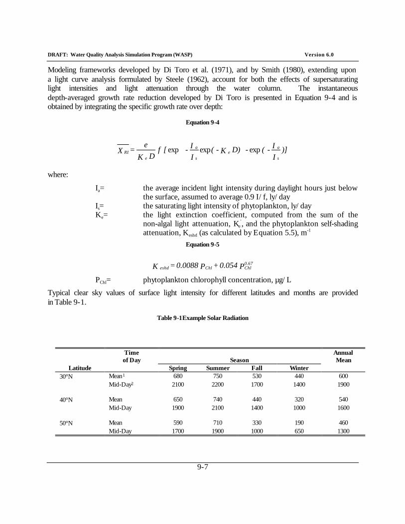
DRAFT: Water Quality Analysis Simulation Program (WASP) Version 6.0
9-7
Modeling frameworks developed by Di Toro et al. (1971), and by Smith (1980), extending upon a light curve analysis formulated by Steele (1962), account for both the effects of supersaturating light intensities and light attenuation through the water column. The instantaneous depth-averaged growth rate reduction developed by Di Toro is presented in Equation 9-4 and is obtained by integrating the specific growth rate over depth:
Equation 9-4
)]II - ( - D) K - (
II - [ f
D K
e = X
s
a e
s
a
e RI expexpexp
where:
Ia= the average incident light intensity during daylight hours just below the surface, assumed to average 0.9 I/f, ly/day
Is= the saturating light intensity of phytoplankton, ly/day Ke= the light extinction coefficient, computed from the sum of the
non-algal light attenuation, Ke', and the phytoplankton self-shading
attenuation, Keshd (as calculated by Equation 5.5), m-1
Equation 9-5
P 0.054 + P 0.0088 = K 0.67ChlChleshd
PChl= phytoplankton chlorophyll concentration, µg/L
Typical clear sky values of surface light intensity for different latitudes and months are provided in Table 9-1.
Table 9-1Example Solar Radiation
Time of Day Season
Annual Mean
Latitude Spring Summer Fall Winter 30°N Mean1 680 750 530 440 600 Mid-Day2 2100 2200 1700 1400 1900 40°N Mean 650 740 440 320 540 Mid-Day 1900 2100 1400 1000 1600 50°N Mean 590 710 330 190 460 Mid-Day 1700 1900 1000 650 1300
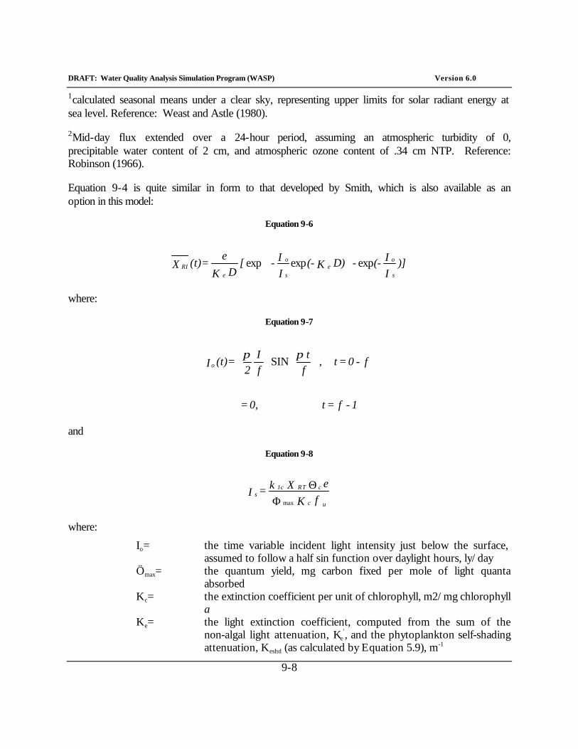
DRAFT: Water Quality Analysis Simulation Program (WASP) Version 6.0
9-8
1calculated seasonal means under a clear sky, representing upper limits for solar radiant energy at sea level. Reference: Weast and Astle (1980).
2Mid-day flux extended over a 24-hour period, assuming an atmospheric turbidity of 0, precipitable water content of 2 cm, and atmospheric ozone content of .34 cm NTP. Reference: Robinson (1966).
Equation 9-4 is quite similar in form to that developed by Smith, which is also available as an option in this model:
Equation 9-6
)]II (- - D) K (-
II - [
D K
e = (t) X
s
o e
s
o
e RI expexpexp
where:
Equation 9-7
1 - f = t 0, =
f - 0 = t ,ft
fI
2
= (t) I o
ππSIN
and
Equation 9-8
f K e X k = Iu c
c RT 1c s
ΦΘ
max
where:
Io= the time variable incident light intensity just below the surface, assumed to follow a half sin function over daylight hours, ly/day
Ömax= the quantum yield, mg carbon fixed per mole of light quanta absorbed
Kc= the extinction coefficient per unit of chlorophyll, m2/mg chlorophyll a
Ke= the light extinction coefficient, computed from the sum of the non-algal light attenuation, Ke
', and the phytoplankton self-shading attenuation, Keshd (as calculated by Equation 5.9), m-1

DRAFT: Water Quality Analysis Simulation Program (WASP) Version 6.0
9-9
Equation 9-9
P K = K Chlceshd
fu= units conversion factor (0.083, assuming 43% incident light is visible and 1 mole photons is equivalent to 52,000 cal), mole photons/m2-ly
Èc= the ratio of carbon to chlorophyll in the phytoplankton, (mg carbon/mg chlorophyll a)
e= the base of natural logarithms (2.71828), unitless
Equations 9.6 - 9.9 give a light limitation coefficient that varies over the day with incident light. This term is numerically integrated over the day within the computer program to obtain daily average light limitation:
Equation 9-10
(t)dt X = X RI
1
o
RI ∫
The term Is, the temperature-dependent light saturation parameter is an unknown in the Di Toro light formulation, and must be determined via the calibration-verification process. In the Smith formulation, this term is calculated from parameters that are reasonably well documented in the literature. As Smith (1980) points out, since the early experiments of Warburg and Negelein (1923), maximum photosynthetic quantum yield (Ömax) has been measured for a wide range of conditions (reviewed by Kok, 1960), and a nearly temperature-independent value of 0.08 to 0.1 mole O2 per mole of photons absorbed is now widely accepted for photosynthesizing plants in general in the laboratory. Bannister (1974a) gives good arguments for adopting 0.06 mole carbon (0.07 mole O2) per mole of photons as the maximum yield for plankton in nature. Reported values for Kc generally fall in the range 0.01 to 0.02 m2mg-1, and 0.016 m2mg-1 has been suggested as the approximate average (Bannister, 1974b).
A second feature incorporated in the modeling framework derived from Smith's work is the calculation of a variable carbon to chlorophyll ratio based on the assumption that adaptive changes in carbon to chlorophyll occur so as to maximize the specific growth rate for ambient conditions of light and temperature. Smith found that phytoplankton adjusts chlorophyll composition so that Is roughly equals 30% of the average available light. The expression used to calculate the carbon to chlorophyll ratio is presented in Equation 9-11 :
Equation 9-11
•
•Φ•ΘD K
e - 1 I e X k
f K 0.3 = e
DK-
aRT 1c
uc c
emax
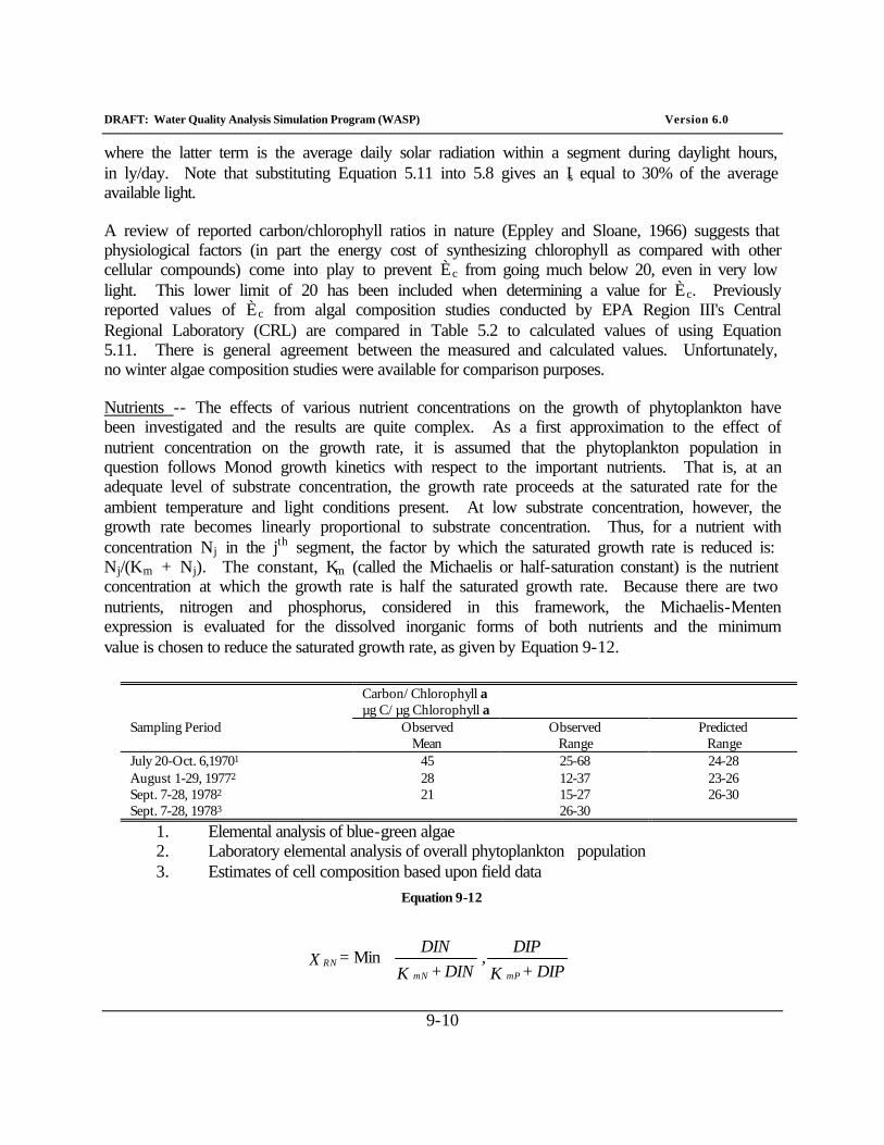
DRAFT: Water Quality Analysis Simulation Program (WASP) Version 6.0
9-10
where the latter term is the average daily solar radiation within a segment during daylight hours, in ly/day. Note that substituting Equation 5.11 into 5.8 gives an Is equal to 30% of the average available light.
A review of reported carbon/chlorophyll ratios in nature (Eppley and Sloane, 1966) suggests that physiological factors (in part the energy cost of synthesizing chlorophyll as compared with other cellular compounds) come into play to prevent Èc from going much below 20, even in very low light. This lower limit of 20 has been included when determining a value for Èc. Previously reported values of Èc from algal composition studies conducted by EPA Region III's Central Regional Laboratory (CRL) are compared in Table 5.2 to calculated values of using Equation 5.11. There is general agreement between the measured and calculated values. Unfortunately, no winter algae composition studies were available for comparison purposes.
Nutrients -- The effects of various nutrient concentrations on the growth of phytoplankton have been investigated and the results are quite complex. As a first approximation to the effect of nutrient concentration on the growth rate, it is assumed that the phytoplankton population in question follows Monod growth kinetics with respect to the important nutrients. That is, at an adequate level of substrate concentration, the growth rate proceeds at the saturated rate for the ambient temperature and light conditions present. At low substrate concentration, however, the growth rate becomes linearly proportional to substrate concentration. Thus, for a nutrient with concentration Nj in the jth segment, the factor by which the saturated growth rate is reduced is: Nj/(Km + Nj). The constant, Km (called the Michaelis or half-saturation constant) is the nutrient concentration at which the growth rate is half the saturated growth rate. Because there are two nutrients, nitrogen and phosphorus, considered in this framework, the Michaelis-Menten expression is evaluated for the dissolved inorganic forms of both nutrients and the minimum value is chosen to reduce the saturated growth rate, as given by Equation 9-12.
Carbon/Chlorophyll a
µg C/µg Chlorophyll a Sampling Period Observed
Mean Observed
Range Predicted
Range July 20-Oct. 6,19701 45 25-68 24-28 August 1-29, 19772 28 12-37 23-26 Sept. 7-28, 19782 21 15-27 26-30 Sept. 7-28, 19783 26-30
1. Elemental analysis of blue-green algae 2. Laboratory elemental analysis of overall phytoplankton population 3. Estimates of cell composition based upon field data
Equation 9-12
DIP + K
DIP ,
DIN + K
DIN = X
mP mN RN Min

DRAFT: Water Quality Analysis Simulation Program (WASP) Version 6.0
9-11
At the user's discretion, the multiplicative formulation for nutrient limitation may be selected. This formulation multiplies the two terms in 5.12. It is not generally recommended.
Figure 9-3 presents plots of G(N) versus DIN and DIP with KmN = 25 µg-N/L and KmP = 1 µg-P/L, respectively. The upper plot shows the standard Michaelis-Menten response curve to various concentrations of the inorganic nutrients. As can be seen, no significant reduction in growth rate is achieved until DIN is less than 200 µg/L (0.2 mg/l) or until DIP is less than 8 µg/L (0.008 mg/l).
The lower plot on Figure 9-3 uses an expanded nutrient scale and shows the Michaelis-Menten formulation in a slightly different format. Here the impact of the function may be evaluated quite readily. For example, a particular reach of the water body may have concentrations of DIN equal to 100 µg/L. This corresponds to a 20% reduction in the growth rate (XRN = 0.8). In order for phosphorus to become the limiting nutrient in the same reach, dissolved inorganic phosphorus must reach a level of 4 µg/L or less. It should also be noted that if upstream nitrogen controls were instituted such that DIN was reduced to 60 µg/L for that same reach, then a further reduction in DIP to 2.5 µg/L would be required to keep phosphorus as the limiting nutrient. In other words, as water column concentrations of DIP begin to approach growth limiting levels due to continued reduction in point source phosphorus effluents, any nitrogen control strategies that might be instituted would require additional levels of phosphorus removal in order to keep phosphorus as the limiting nutrient.
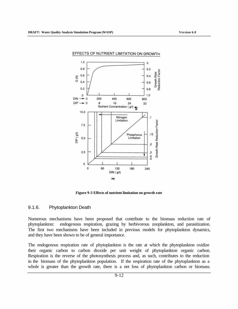
DRAFT: Water Quality Analysis Simulation Program (WASP) Version 6.0
9-12
Figure 9-3 Effects of nutrient limitation on growth rate
9.1.6. Phytoplankton Death
Numerous mechanisms have been proposed that contribute to the biomass reduction rate of phytoplankton: endogenous respiration, grazing by herbivorous zooplankton, and parasitization. The first two mechanisms have been included in previous models for phytoplankton dynamics, and they have been shown to be of general importance.
The endogenous respiration rate of phytoplankton is the rate at which the phytoplankton oxidize their organic carbon to carbon dioxide per unit weight of phytoplankton organic carbon. Respiration is the reverse of the photosynthesis process and, as such, contributes to the reduction in the biomass of the phytoplankton population. If the respiration rate of the phytoplankton as a whole is greater than the growth rate, there is a net loss of phytoplankton carbon or biomass.
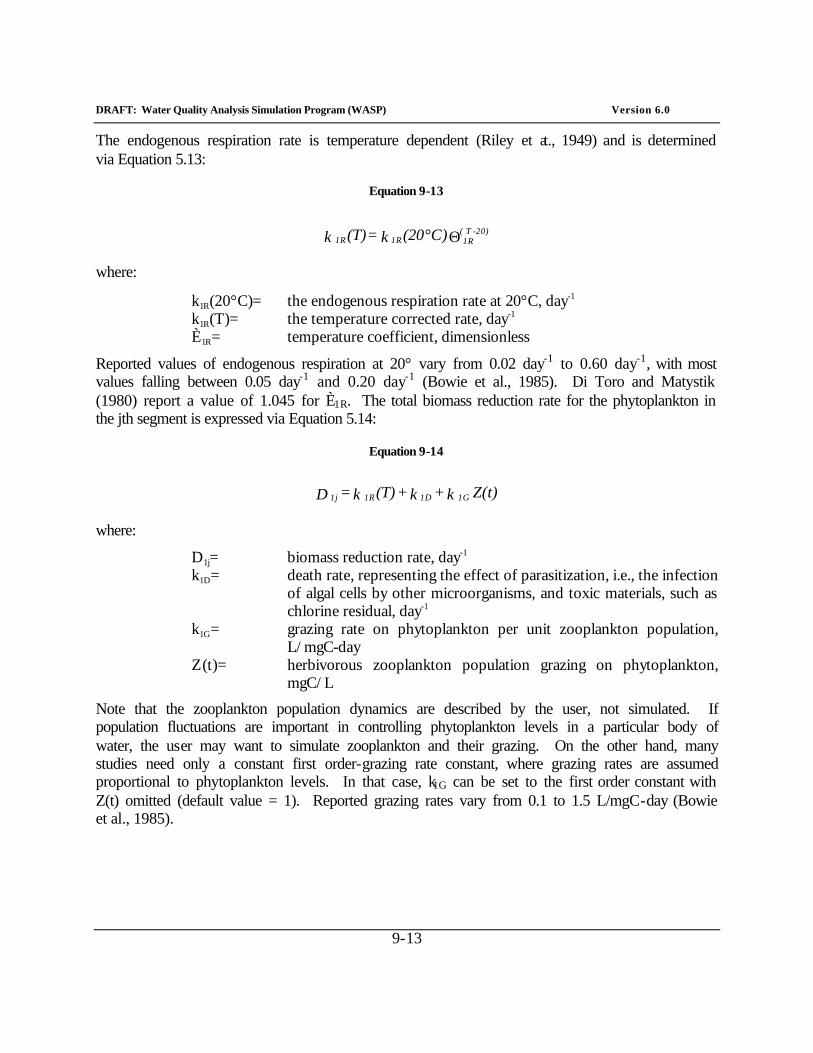
DRAFT: Water Quality Analysis Simulation Program (WASP) Version 6.0
9-13
The endogenous respiration rate is temperature dependent (Riley et at., 1949) and is determined via Equation 5.13:
Equation 9-13
Θ° 20)-T (1R 1R 1R C)(20k = (T)k
where:
k1R(20°C)= the endogenous respiration rate at 20°C, day-1 k1R(T)= the temperature corrected rate, day-1 È1R= temperature coefficient, dimensionless
Reported values of endogenous respiration at 20° vary from 0.02 day-1 to 0.60 day-1, with most values falling between 0.05 day-1 and 0.20 day-1 (Bowie et al., 1985). Di Toro and Matystik (1980) report a value of 1.045 for È1R. The total biomass reduction rate for the phytoplankton in the jth segment is expressed via Equation 5.14:
Equation 9-14
Z(t)k + k + (T)k = D 1G 1D 1R 1j
where:
D1j= biomass reduction rate, day-1 k1D= death rate, representing the effect of parasitization, i.e., the infection
of algal cells by other microorganisms, and toxic materials, such as chlorine residual, day-1
k1G= grazing rate on phytoplankton per unit zooplankton population, L/mgC-day
Z(t)= herbivorous zooplankton population grazing on phytoplankton, mgC/L
Note that the zooplankton population dynamics are described by the user, not simulated. If population fluctuations are important in controlling phytoplankton levels in a particular body of water, the user may want to simulate zooplankton and their grazing. On the other hand, many studies need only a constant first order-grazing rate constant, where grazing rates are assumed proportional to phytoplankton levels. In that case, k1G can be set to the first order constant with Z(t) omitted (default value = 1). Reported grazing rates vary from 0.1 to 1.5 L/mgC-day (Bowie et al., 1985).
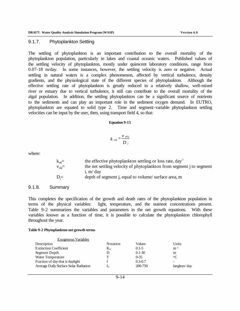
DRAFT: Water Quality Analysis Simulation Program (WASP) Version 6.0
9-14
9.1.7. Phytoplankton Settling
The settling of phytoplankton is an important contribution to the overall mortality of the phytoplankton population, particularly in lakes and coastal oceanic waters. Published values of the settling velocity of phytoplankton, mostly under quiescent laboratory conditions, range from 0.07-18 m/day. In some instances, however, the settling velocity is zero or negative. Actual settling in natural waters is a complex phenomenon, affected by vertical turbulence, density gradients, and the physiological state of the different species of phytoplankton. Although the effective settling rate of phytoplankton is greatly reduced in a relatively shallow, well-mixed river or estuary due to vertical turbulence, it still can contribute to the overall mortality of the algal population. In addition, the settling phytoplankton can be a significant source of nutrients to the sediments and can play an important role in the sediment oxygen demand. In EUTRO, phytoplankton are equated to solid type 2. Time and segment-variable phytoplankton settling velocities can be input by the user, then, using transport field 4, so that:
Equation 9-15
Dv = k
j
s4ij s4j
where:
ks4j= the effective phytoplankton settling or loss rate, day-1 vs4ij= the net settling velocity of phytoplankton from segment j to segment
i, m/day Dj= depth of segment j, equal to volume/surface area, m
9.1.8. Summary
This completes the specification of the growth and death rates of the phytoplankton population in terms of the physical variables: light, temperature, and the nutrient concentrations present. Table 9-2 summarizes the variables and parameters in the net growth equations. With these variables known as a function of time, it is possible to calculate the phytoplankton chlorophyll throughout the year.
Table 9-2 Phytoplankton net growth terms
Exogenous Variables Description Notation Values Units Extinction Coefficient Ke 0.1-5 m -1 Segment Depth D 0.1-30 m Water Temperature T 0-35 oC Fraction of day that is daylight f 0.3-0.7 - Average Daily Surface Solar Radiation Ia 200-750 langleys/day
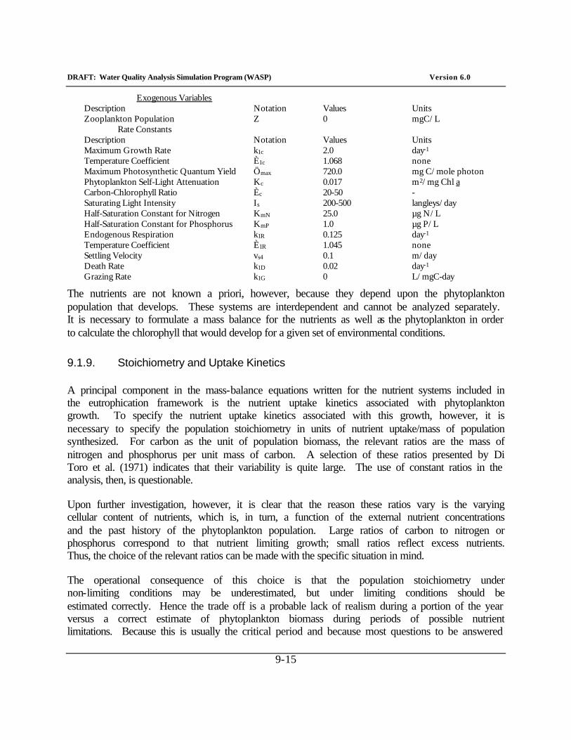
DRAFT: Water Quality Analysis Simulation Program (WASP) Version 6.0
9-15
Exogenous Variables Description Notation Values Units Zooplankton Population Z 0 mgC/L Rate Constants Description Notation Values Units Maximum Growth Rate k1c 2.0 day-1 Temperature Coefficient È1c 1.068 none Maximum Photosynthetic Quantum Yield Ömax 720.0 mg C/mole photon Phytoplankton Self-Light Attenuation Kc 0.017 m2/mg Chl a Carbon-Chlorophyll Ratio Èc 20-50 - Saturating Light Intensity Is 200-500 langleys/day Half-Saturation Constant for Nitrogen KmN 25.0 µg N/L Half-Saturation Constant for Phosphorus KmP 1.0 µg P/L Endogenous Respiration k1R 0.125 day-1 Temperature Coefficient È1R 1.045 none Settling Velocity vs4 0.1 m/day Death Rate k1D 0.02 day-1 Grazing Rate k1G 0 L/mgC-day
The nutrients are not known a priori, however, because they depend upon the phytoplankton population that develops. These systems are interdependent and cannot be analyzed separately. It is necessary to formulate a mass balance for the nutrients as well as the phytoplankton in order to calculate the chlorophyll that would develop for a given set of environmental conditions.
9.1.9. Stoichiometry and Uptake Kinetics
A principal component in the mass-balance equations written for the nutrient systems included in the eutrophication framework is the nutrient uptake kinetics associated with phytoplankton growth. To specify the nutrient uptake kinetics associated with this growth, however, it is necessary to specify the population stoichiometry in units of nutrient uptake/mass of population synthesized. For carbon as the unit of population biomass, the relevant ratios are the mass of nitrogen and phosphorus per unit mass of carbon. A selection of these ratios presented by Di Toro et al. (1971) indicates that their variability is quite large. The use of constant ratios in the analysis, then, is questionable.
Upon further investigation, however, it is clear that the reason these ratios vary is the varying cellular content of nutrients, which is, in turn, a function of the external nutrient concentrations and the past history of the phytoplankton population. Large ratios of carbon to nitrogen or phosphorus correspond to that nutrient limiting growth; small ratios reflect excess nutrients. Thus, the choice of the relevant ratios can be made with the specific situation in mind.
The operational consequence of this choice is that the population stoichiometry under non-limiting conditions may be underestimated, but under limiting conditions should be estimated correctly. Hence the trade off is a probable lack of realism during a portion of the year versus a correct estimate of phytoplankton biomass during periods of possible nutrient limitations. Because this is usually the critical period and because most questions to be answered
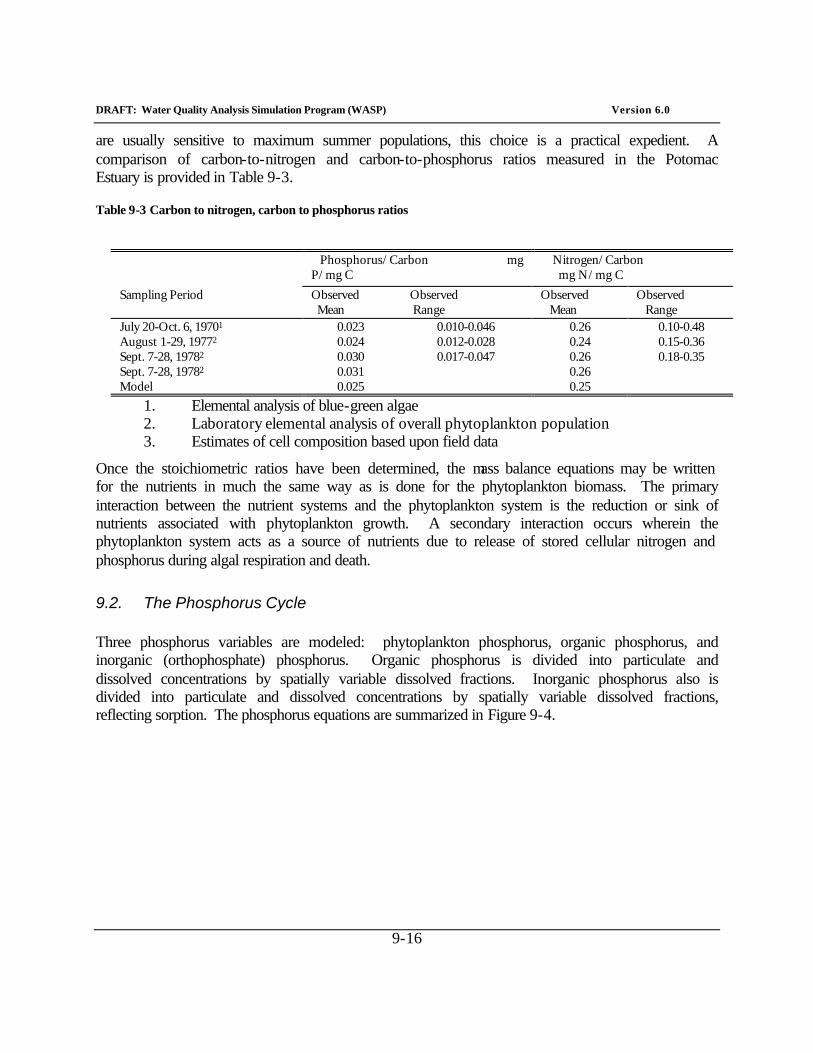
DRAFT: Water Quality Analysis Simulation Program (WASP) Version 6.0
9-16
are usually sensitive to maximum summer populations, this choice is a practical expedient. A comparison of carbon-to-nitrogen and carbon-to-phosphorus ratios measured in the Potomac Estuary is provided in Table 9-3.
Table 9-3 Carbon to nitrogen, carbon to phosphorus ratios
Phosphorus/Carbon mg P/mg C
Nitrogen/Carbon mg N/mg C
Sampling Period Observed Mean
Observed Range
Observed Mean
Observed Range
July 20-Oct. 6, 19701 0.023 0.010-0.046 0.26 0.10-0.48 August 1-29, 19772 0.024 0.012-0.028 0.24 0.15-0.36 Sept. 7-28, 19782 0.030 0.017-0.047 0.26 0.18-0.35 Sept. 7-28, 19782 0.031 0.26 Model 0.025 0.25
1. Elemental analysis of blue-green algae 2. Laboratory elemental analysis of overall phytoplankton population 3. Estimates of cell composition based upon field data
Once the stoichiometric ratios have been determined, the mass balance equations may be written for the nutrients in much the same way as is done for the phytoplankton biomass. The primary interaction between the nutrient systems and the phytoplankton system is the reduction or sink of nutrients associated with phytoplankton growth. A secondary interaction occurs wherein the phytoplankton system acts as a source of nutrients due to release of stored cellular nitrogen and phosphorus during algal respiration and death.
9.2. The Phosphorus Cycle
Three phosphorus variables are modeled: phytoplankton phosphorus, organic phosphorus, and inorganic (orthophosphate) phosphorus. Organic phosphorus is divided into particulate and dissolved concentrations by spatially variable dissolved fractions. Inorganic phosphorus also is divided into particulate and dissolved concentrations by spatially variable dissolved fractions, reflecting sorption. The phosphorus equations are summarized in Figure 9-4.
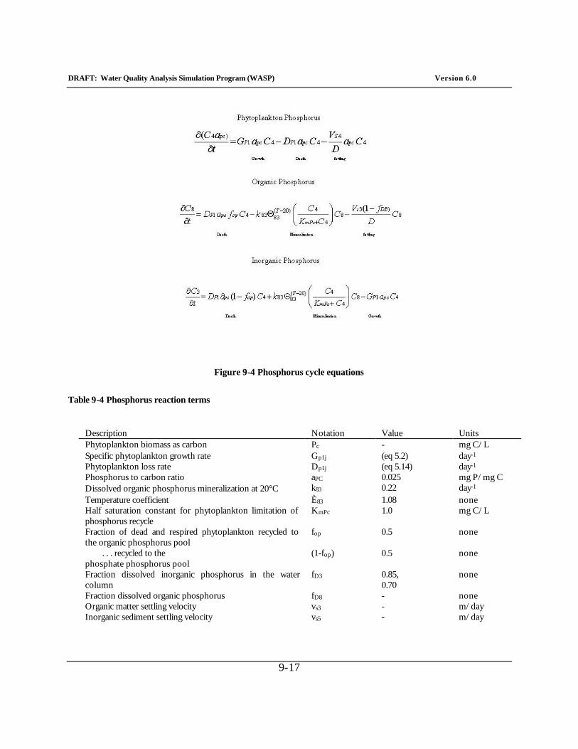
DRAFT: Water Quality Analysis Simulation Program (WASP) Version 6.0
9-17
Figure 9-4 Phosphorus cycle equations
Table 9-4 Phosphorus reaction terms
Description Notation Value Units Phytoplankton biomass as carbon Pc - mg C/L Specific phytoplankton growth rate Gp1j (eq 5.2) day-1 Phytoplankton loss rate Dp1j (eq 5.14) day-1 Phosphorus to carbon ratio aPC 0.025 mg P/mg C Dissolved organic phosphorus mineralization at 20°C k83 0.22 day-1 Temperature coefficient È83 1.08 none Half saturation constant for phytoplankton limitation of phosphorus recycle
KmPc 1.0 mg C/L
Fraction of dead and respired phytoplankton recycled to the organic phosphorus pool
fop 0.5 none
. . . recycled to the phosphate phosphorus pool
(1-fop) 0.5 none
Fraction dissolved inorganic phosphorus in the water column
fD3 0.85, 0.70
none
Fraction dissolved organic phosphorus fD8 - none Organic matter settling velocity vs3 - m/day Inorganic sediment settling velocity vs5 - m/day
DRAFT: Water Quality Analysis Simulation Program (WASP) Version 6.0
9-18
9.2.1. Phytoplankton Growth
As phytoplankton grow, dissolved inorganic phosphorus is taken up, stored and incorporated into biomass. For every mg of phytoplankton carbon produced, aPC mg of inorganic phosphorus is taken up.
9.2.2. Phytoplankton Death
As phytoplankton respire and die, biomass is recycled to nonliving organic and inorganic matter. For every mg of phytoplankton carbon consumed or lost, aPC mg of phosphorus is released. A fraction fop is organic, while (1 - fop) is in the inorganic form and readily available for uptake by other viable algal cells. In work on the Great Lakes, fop was assigned at 50% (Di Toro and Matystik, 1980).
9.2.3. Mineralization
Nonliving organic phosphorus must undergo mineralization or bacterial decomposition into inorganic phosphorus before utilization by phytoplankton. In their work on Lake Huron and Saginaw Bay, Di Toro and Matystik (1980) proposed a nutrient recycle formulation that was a function of the localized phytoplankton population. This proposal was based on both an analysis of available field data and the work of others (Hendry, 1977; Lowe, 1976; Henrici, 1938; Menon, 1972; and Rao, 1976) that indicated bacterial biomass increased as phytoplankton biomass increased. EUTRO uses a saturating recycle mechanism, a compromise between conventional first-order kinetics and a second order recycle mechanism wherein the recycle rate is directly proportional to the phytoplankton biomass present, as had been indicated in pure culture, bacteria-seeded, laboratory studies (Jewell and McCarty, 1971).
Saturating recycle permits second order dependency at low phytoplankton concentrations, when Pc << KmPc, where KmPc is the half-saturation constant for recycle, and permits first order recycle when the phytoplankton greatly exceed the half-saturation constant. Basically, this mechanism slows the recycle rate if the phytoplankton population is small, but does not permit the rate to increase continuously as phytoplankton increase. The assumption is that at higher population levels, recycle kinetics proceed at the maximum first order rate. The default value for KmPc is 0, which causes mineralization to proceed at its first order rate at all phytoplankton levels.
9.2.4. Sorption
There is an adsorption-desorption interaction between dissolved inorganic phosphorus and suspended particulate matter in the water column. The subsequent settling of the suspended solids together with the sorbed inorganic phosphorus can act as a significant loss mechanism in the water column and is a source of phosphorus to the sediment. Because the rates of reaction
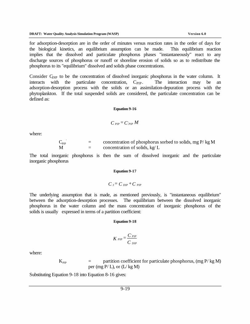
DRAFT: Water Quality Analysis Simulation Program (WASP) Version 6.0
9-19
for adsorption-desorption are in the order of minutes versus reaction rates in the order of days for the biological kinetics, an equilibrium assumption can be made. This equilibrium reaction implies that the dissolved and particulate phosphorus phases "instantaneously" react to any discharge sources of phosphorus or runoff or shoreline erosion of solids so as to redistribute the phosphorus to its "equilibrium" dissolved and solids phase concentrations.
Consider CDIP to be the concentration of dissolved inorganic phosphorus in the water column. It interacts with the particulate concentration, CPIP . The interaction may be an adsorption-desorption process with the solids or an assimilation-depuration process with the phytoplankton. If the total suspended solids are considered, the particulate concentration can be defined as:
Equation 9-16
MC = C ,PIP PIP
where:
CPIP' = concentration of phosphorus sorbed to solids, mg P/kg M
M = concentration of solids, kg/L
The total inorganic phosphorus is then the sum of dissolved inorganic and the particulate inorganic phosphorus
Equation 9-17
C + C = C PIP DIP 3
The underlying assumption that is made, as mentioned previously, is "instantaneous equilibrium" between the adsorption-desorption processes. The equilibrium between the dissolved inorganic phosphorus in the water column and the mass concentration of inorganic phosphorus of the solids is usually expressed in terms of a partition coefficient:
Equation 9-18
CC = K
DIP
,PIP
PIP
where:
KPIP = partition coefficient for particulate phosphorus, (mg P/kg M) per (mg P/L), or (L/kg M)
Substituting Equation 9-18 into Equation 8-16 gives:
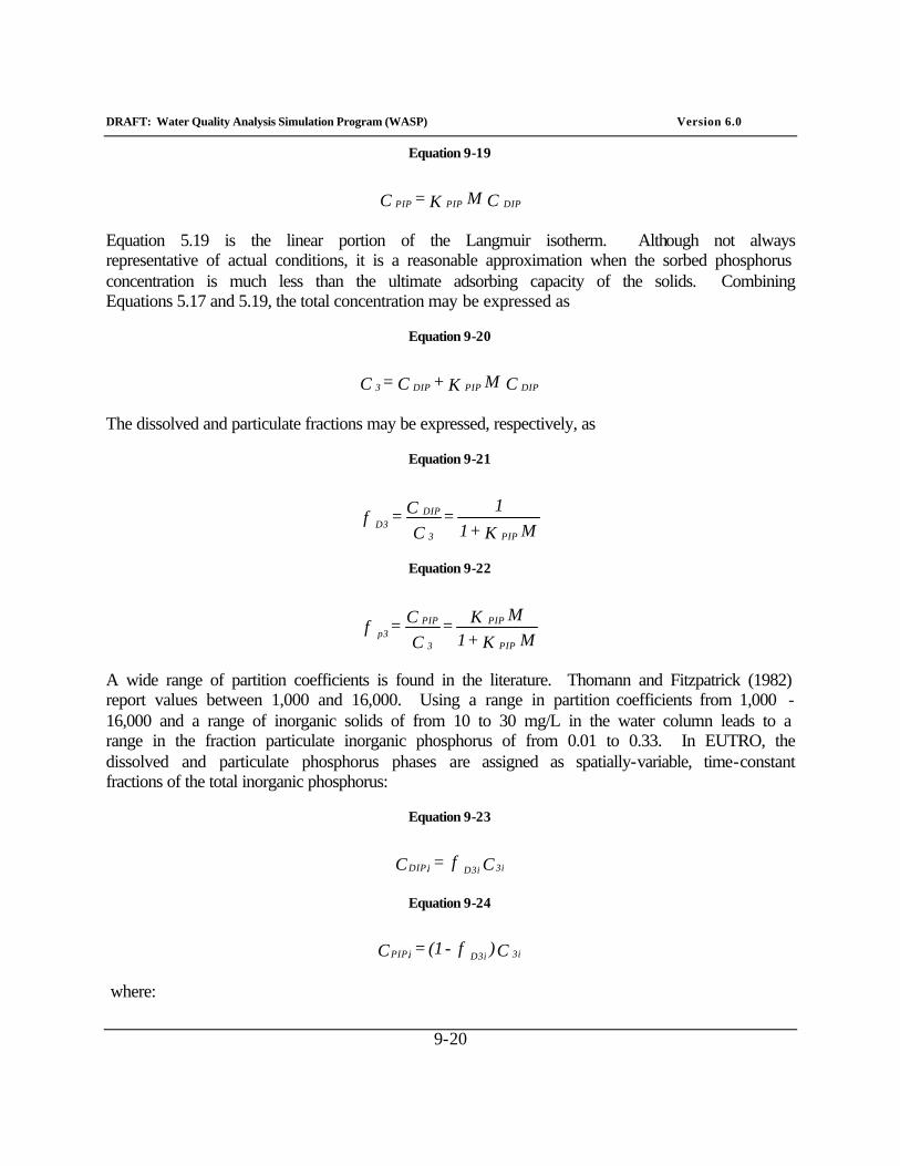
DRAFT: Water Quality Analysis Simulation Program (WASP) Version 6.0
9-20
Equation 9-19
C MK = C DIP PIP PIP
Equation 5.19 is the linear portion of the Langmuir isotherm. Although not always representative of actual conditions, it is a reasonable approximation when the sorbed phosphorus concentration is much less than the ultimate adsorbing capacity of the solids. Combining Equations 5.17 and 5.19, the total concentration may be expressed as
Equation 9-20
C MK + C = C DIP PIP DIP 3
The dissolved and particulate fractions may be expressed, respectively, as
Equation 9-21
MK + 11
= C
C = fPIP 3
DIP D3
Equation 9-22
MK + 1 MK =
CC = f
PIP
PIP
3
PIP p3
A wide range of partition coefficients is found in the literature. Thomann and Fitzpatrick (1982) report values between 1,000 and 16,000. Using a range in partition coefficients from 1,000 - 16,000 and a range of inorganic solids of from 10 to 30 mg/L in the water column leads to a range in the fraction particulate inorganic phosphorus of from 0.01 to 0.33. In EUTRO, the dissolved and particulate phosphorus phases are assigned as spatially-variable, time-constant fractions of the total inorganic phosphorus:
Equation 9-23
C f = C 3iD3i iDIP,
Equation 9-24
C )f - (1 = C 3i D3i iPIP,
where:
DRAFT: Water Quality Analysis Simulation Program (WASP) Version 6.0
9-21
C3i= the total inorganic phosphorus in segment i, mg/L fD3i= the fraction of the total inorganic phosphorus assigned to the
dissolved phase in segment i CDIP,i= the equilibrium dissolved inorganic phosphorus in segment i,
available for algal uptake, mg/L CPIP,i= the equilibrium sorbed inorganic phosphorus in segment i, which
may then settle to the sediment layer from the water column, mg/L.
9.2.5. Settling
Particulate organic and inorganic phosphorus settle according to user-specified velocities and particulate fractions. Particulate organic phosphorus is equated to solid type 1, which represents organic matter. Time and segment-variable organic matter settling velocities, vs3, can be input by the user using transport field 3. Segment-variable organic phosphorus dissolved fractions, fD8j, are input with initial conditions.
Particulate inorganic phosphorus is equated to solid type 3, which represents inorganic sediment. Time and segment variable inorganic phosphorus settling velocities, vs5, can be input by the user using transport field 5. Segment-variable inorganic phosphorus dissolved fractions, fD3, are input with initial conditions.
9.3. The Nitrogen Cycle
Four nitrogen variables are modeled: phytoplankton nitrogen, organic nitrogen, ammonia, and nitrate. A summary is illustrated in Figure 9-5. Table 9-5 summarizes the terms used in the nitrogen system kinetics.
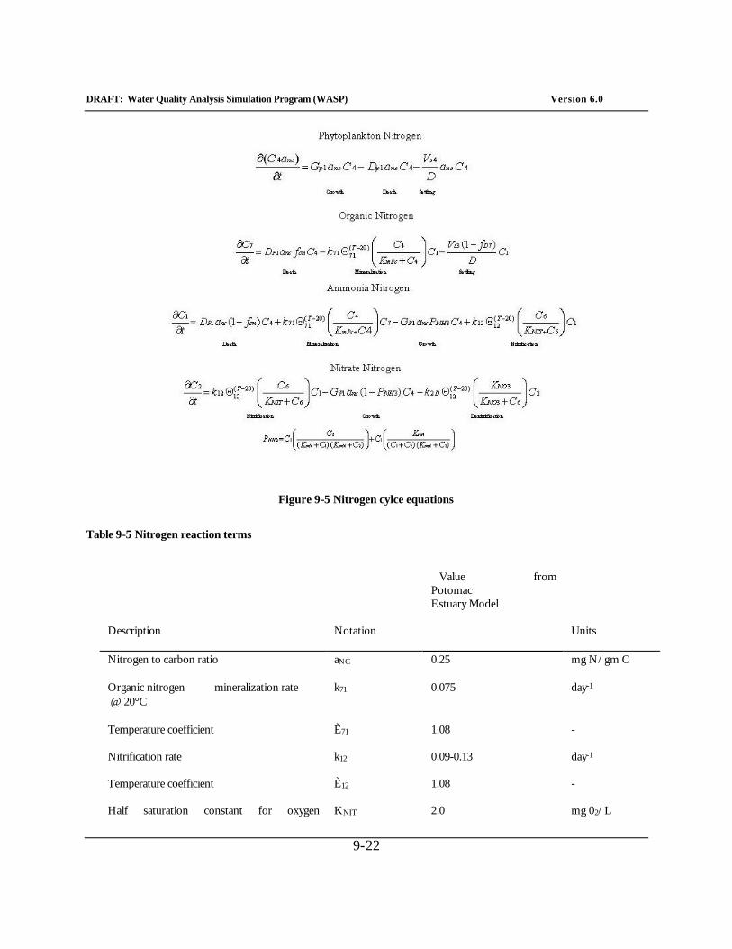
DRAFT: Water Quality Analysis Simulation Program (WASP) Version 6.0
9-22
Figure 9-5 Nitrogen cylce equations
Table 9-5 Nitrogen reaction terms
Value from
Potomac Estuary Model
Description
Notation
Units
Nitrogen to carbon ratio
aNC
0.25
mg N/gm C
Organic nitrogen mineralization rate @ 20°C
k71
0.075
day-1
Temperature coefficient
È71
1.08
-
Nitrification rate
k12
0.09-0.13
day-1
Temperature coefficient
È12
1.08
-
Half saturation constant for oxygen KNIT 2.0 mg 02/L
DRAFT: Water Quality Analysis Simulation Program (WASP) Version 6.0
9-23
limitation of nitrification
Denitrification rate at 20°C
k2D
0.09
day-1
Temperature coefficient
È2D
1.045
-
Michaelis constant for denitrification
KNO3
0.1
mg O2/L
Fraction of dead and respired phytoplankton recycled ...
to the organic nitrogen pool
fON
0.5
-
to the ammonia nitrogen pool
(1-fON)
0.5
-
Preference for ammonia uptake term
PNH3
eq. 5.30
-
Fraction dissolved organic nitrogen
fD7
1.0
-
Organic matter settling velocity
vs3
-
m/day
9.3.1. Phytoplankton Growth
As phytoplankton grow, dissolved inorganic nitrogen is taken up and incorporated into biomass. For every mg of phytoplankton carbon produced, aNC mg of inorganic nitrogen is taken up. Both ammonia and nitrate are available for uptake and use in cell growth by phytoplankton; however, for physiological reasons, the preferred form is ammonia nitrogen. The ammonia preference term PNH3 is given in Figure 9-6.
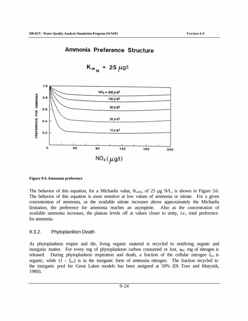
DRAFT: Water Quality Analysis Simulation Program (WASP) Version 6.0
9-24
Figure 9-6 Ammonia preference
The behavior of this equation, for a Michaelis value, KmN, of 25 µg N/L, is shown in Figure 5.6. The behavior of this equation is most sensitive at low values of ammonia or nitrate. For a given concentration of ammonia, as the available nitrate increases above approximately the Michaelis limitation, the preference for ammonia reaches an asymptote. Also as the concentration of available ammonia increases, the plateau levels off at values closer to unity, i.e., total preference for ammonia.
9.3.2. Phytoplankton Death
As phytoplankton respire and die, living organic material is recycled to nonliving organic and inorganic matter. For every mg of phytoplankton carbon consumed or lost, aNC mg of nitrogen is released. During phytoplankton respiration and death, a fraction of the cellular nitrogen fon is organic, while (1 - fon) is in the inorganic form of ammonia nitrogen. The fraction recycled to the inorganic pool for Great Lakes models has been assigned at 50% (Di Toro and Matystik, 1980).
DRAFT: Water Quality Analysis Simulation Program (WASP) Version 6.0
9-25
9.3.3. Mineralization
Nonliving organic nitrogen must undergo mineralization or bacterial decomposition into ammonia nitrogen before utilization by phytoplankton. In EUTRO, the first order, temperature-corrected rate constant is modified by a saturated recycle term, as explained in the phosphorus mineralization section. This mechanism slows the mineralization rate if the phytoplankton population is small, but does not permit the rate to increase continuously as phytoplankton increase. The default value for the half-saturation constant KmPc is 0, which causes mineralization to proceed at its first order rate at all phytoplankton levels.
9.3.4. Settling
Particulate organic nitrogen settles according to user-specified velocities and particulate fractions. Particulate organic nitrogen is equated to solid type 1, which represents organic matter. Time and segment-variable organic matter settling velocities, vs3, can be input by the user using transport field 3. Segment-variable organic nitrogen dissolved fractions, fD7, are input with initial conditions.
9.3.5. Nitrification
Ammonia nitrogen, in the presence of nitrifying bacteria and oxygen, is converted to nitrate nitrogen (nitrification). The process of nitrification in natural waters is carried out by aerobic autotrophs; Nitrosomonas and Nitrobacter predominate in fresh waters. It is a two-step process with Nitrosomonas bacteria responsible for the conversion of ammonia to nitrite and Nitrobacter responsible for the conversion of nitrite to nitrate.
Essential to this reaction process are aerobic conditions. Also this process appears to be affected by high or low values of pH that inhibit Nitrosomonas growth, particularly for pH below 7 and greater than 9. As with phytoplankton, the nitrifying bacterial populations are sensitive to flow. During periods of high flow or storm runoff, upstream bacteria may be advected downstream, with some lag time after a flow transient before they can build up to significant levels again.
The process of nitrification in natural waters, then, is complex, depending on dissolved oxygen, pH, and flow conditions, which in turn leads to spatially and temporally varying rates of nitrification. To properly account for this complex phenomenon in the modeling framework would be difficult and would require a database that is usually unavailable.
The kinetic expression for nitrification in EUTRO contains three terms -- a first order rate constant, a temperature correction term, and a low DO correction term. The first two terms are standard. The third term represents the decline of the nitrification rate as DO levels approach 0. The user may specify the half-saturation constant KNIT , which represents the DO level at which
DRAFT: Water Quality Analysis Simulation Program (WASP) Version 6.0
9-26
the nitrification rate is reduced by half. The default value is zero, which allows this reaction to proceed fully even under anaerobic conditions.
9.3.6. Denitrification
Denitrification refers to the reduction of NO3 (or NO2) to N2 and other gaseous products such as N2O and NO. This process is carried out by a large number of heterotrophic, facultative anaerobes. Under normal aerobic conditions found in the water column, these organisms use oxygen to oxidize organic material. Under the anaerobic conditions found in the sediment bed or during extremely low oxygen conditions in the water column, however, these organisms are able to use NO3 as the electron acceptor.
The process of denitrification is included in the modeling framework simply as a sink of nitrate. The kinetic expression for denitrification in EUTRO contains three terms -- a first order rate constant, a temperature correction term, and a DO correction term. The first two terms are standard. The third term represents the decline of the denitrification rate as DO levels rise above 0. The user may specify the half-saturation constant KNO3, which represents the DO level at which the denitrification rate is reduced by half. The default value is zero, which prevents this reaction at all DO levels. Denitrification is assumed to always occur in the sediment layer where anaerobic conditions always exist.
9.4. The Dissolved Oxygen Balance
Five state variables participate in the DO balance: phytoplankton carbon, ammonia, nitrate, carbonaceous biochemical oxygen demand, and dissolved oxygen. A summary is illustrated in Figure 9-1. The reduction of dissolved oxygen is a consequence of the aerobic respiratory processes in the water column and the anaerobic processes in the underlying sediments. Both these processes contribute significantly and, therefore, it is necessary to formulate their kinetics explicitly.
The dissolved oxygen processes in EUTRO are discussed in Chapter 8. The CBOD and DO reaction terms are summarized in Table 8-1.
9.4.1. Benthic - Water Column Interactions
The decomposition of organic material in benthic sediment can have profound effects on the concentrations of oxygen and nutrients in the overlying waters. The decomposition of organic material releases nutrients to the sediment interstitial waters and also results in the exertion of an oxygen demand at the sediment-water interface. As a result, the areal fluxes from the sediment can be substantial nutrient sources or oxygen sinks to the overlying water column. Additionally, the occurrence of anoxia, due in part to the sediment oxygen demand, may dramatically increase
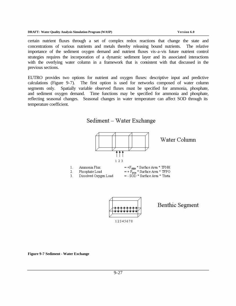
DRAFT: Water Quality Analysis Simulation Program (WASP) Version 6.0
9-27
certain nutrient fluxes through a set of complex redox reactions that change the state and concentrations of various nutrients and metals thereby releasing bound nutrients. The relative importance of the sediment oxygen demand and nutrient fluxes vis-a-vis future nutrient control strategies requires the incorporation of a dynamic sediment layer and its associated interactions with the overlying water column in a framework that is consistent with that discussed in the previous sections.
EUTRO provides two options for nutrient and oxygen fluxes: descriptive input and predictive calculations (Figure 9-7). The first option is used for networks composed of water column segments only. Spatially variable observed fluxes must be specified for ammonia, phosphate, and sediment oxygen demand. Time functions may be specified for ammonia and phosphate, reflecting seasonal changes. Seasonal changes in water temperature can affect SOD through its temperature coefficient.
Figure 9-7 Sediment - Water Exchange
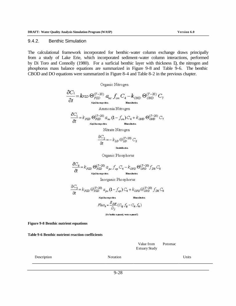
DRAFT: Water Quality Analysis Simulation Program (WASP) Version 6.0
9-28
9.4.2. Benthic Simulation
The calculational framework incorporated for benthic-water column exchange draws principally from a study of Lake Erie, which incorporated sediment-water column interactions, performed by Di Toro and Connolly (1980). For a surficial benthic layer with thickness Dj, the nitrogen and phosphorus mass balance equations are summarized in Figure 9-8 and Table 9-6. The benthic CBOD and DO equations were summarized in Figure 8-4 and Table 8-2 in the previous chapter.
Figure 9-8 Benthic nutrient equations
Table 9-6 Benthic nutrient reaction coefficients
Value from Potomac Estuary Study
Description
Notation
Units
DRAFT: Water Quality Analysis Simulation Program (WASP) Version 6.0
9-29
Value from Potomac Estuary Study
Anaerobic algal decomposition rate
kPZD
0.02
day-1
Temperature coefficient
ÈPZD
1.08
none
Organic nitrogen decomposition rate
kOND
0.0004
day-1
Temperature coefficient
ÈOND
1.08
none
Organic phosphorus decomposition rate
kOPD
0.0004
day-1
Temperature coefficient
ÈOPD
1.08
none
Fraction inorganic phosphorus dissolved in benthic layer
fD3j
0.045-0.001
none
Diffusive exchange coefficient
EDIF
2-2.5 x 10⁻⁴
m2/day
Benthic layer depth
Dj
0.1-0.3
m
Benthic layer
j
Water column
i
WASP6 allows a more detailed parameterization of settling into the benthos that includes not only a downward settling velocity but an upward resuspension velocity as well. In this context, then, the net particulate flux to the sediment is due to the difference between the downward settling flux and the upward resuspension flux.
Benthic Depth -- One of the first decisions to be made regarding the benthic layer is to determine its depth. Two factors influence this decision. The first is to adequately reflect the thickness of the active layer, the depth to which the sediment is influenced by exchange with the overlying water column. Secondly one wishes the model to reflect a reasonable time history or "memory" in the sediment layer. Too thin a layer and the benthos will "remember" or be influenced by deposition of material that would have occurred only within the last year or two of the period being analyzed; too thick a layer and the model will "average" too long a history, not reflecting, as in the case of phosphorus, substantial reductions in sedimentary phosphorus resulting from reduced phosphorus discharges from sewage treatment plants. The choice of sediment thickness is further complicated by spatially variable sedimentation rates. The benthic layer depths, together with the assigned sedimentation velocities, provide for a multi-year detention time or "memory", providing a reasonable approximation of the active layer in light of the observed pore water gradients.
Benthic Nitrogen -- The next consideration is the application of these mass balance equations to the nitrogen species in a reducing sediment (Berner, 1974). Particulate organic nitrogen is
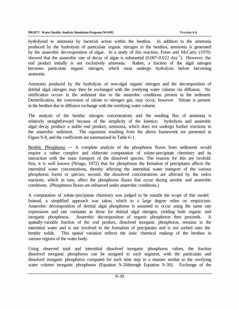
DRAFT: Water Quality Analysis Simulation Program (WASP) Version 6.0
9-30
hydrolyzed to ammonia by bacterial action within the benthos. In addition to the ammonia produced by the hydrolysis of particulate organic nitrogen in the benthos, ammonia is generated by the anaerobic decomposition of algae. In a study of this reaction, Foree and McCarty (1970) showed that the anaerobic rate of decay of algae is substantial (0.007-0.022 day-1). However, the end product initially is not exclusively ammonia. Rather, a fraction of the algal nitrogen becomes particulate organic nitrogen, which must undergo hydrolysis before becoming ammonia.
Ammonia produced by the hydrolysis of non-algal organic nitrogen and the decomposition of detrital algal nitrogen may then be exchanged with the overlying water column via diffusion. No nitrification occurs in the sediment due to the anaerobic conditions present in the sediment. Denitrification, the conversion of nitrate to nitrogen gas, may occur, however. Nitrate is present in the benthos due to diffusive exchange with the overlying water column.
The analysis of the benthic nitrogen concentrations and the resulting flux of ammonia is relatively straightforward because of the simplicity of the kinetics: hydrolysis and anaerobic algal decay produce a stable end product, ammonia, which does not undergo further reactions in the anaerobic sediment. The equations resulting from the above framework are presented in Figure 9-8, and the coefficients are summarized in Table 6-1.
Benthic Phosphorus -- A complete analysis of the phosphorus fluxes from sediments would require a rather complex and elaborate computation of solute-precipitate chemistry and its interaction with the mass transport of the dissolved species. The reasons for this are twofold: first, it is well known (Nriagu, 1972) that for phosphorus the formation of precipitates affects the interstitial water concentrations, thereby affecting the interstitial water transport of the various phosphorus forms or species; second, the dissolved concentrations are affected by the redox reactions, which in turn, affect the phosphorus fluxes that occur during aerobic and anaerobic conditions. (Phosphorus fluxes are enhanced under anaerobic conditions.)
A computation of solute-precipitate chemistry was judged to be outside the scope of this model. Instead, a simplified approach was taken, which to a large degree relies on empiricism. Anaerobic decomposition of detrital algal phosphorus is assumed to occur using the same rate expressions and rate constants as those for detrital algal nitrogen, yielding both organic and inorganic phosphorus. Anaerobic decomposition of organic phosphorus then proceeds. A spatially-variable fraction of the end product, dissolved inorganic phosphorus, remains in the interstitial water and is not involved in the formation of precipitates and is not sorbed onto the benthic solids. This spatial variation reflects the ionic chemical makeup of the benthos in various regions of the water body.
Using observed total and interstitial dissolved inorganic phosphorus values, the fraction dissolved inorganic phosphorus can be assigned to each segment, with the particulate and dissolved inorganic phosphorus computed for each time step in a manner similar to the overlying water column inorganic phosphorus (Equation 9-26through Equation 9-30). Exchange of the
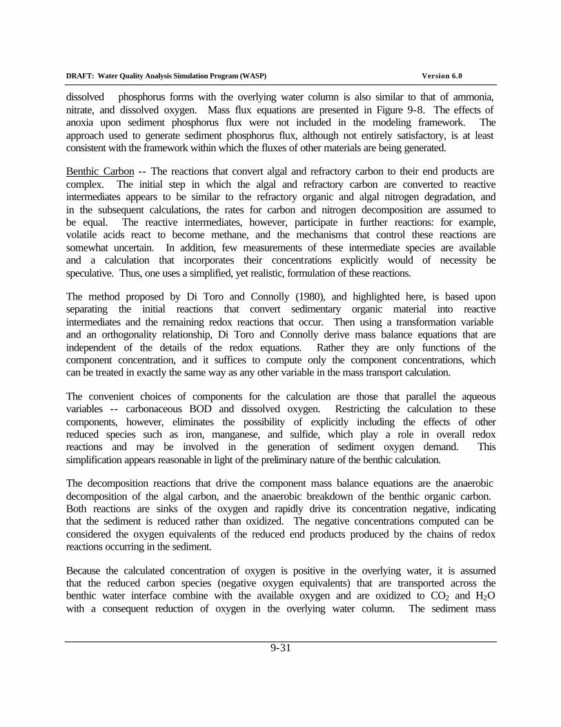
DRAFT: Water Quality Analysis Simulation Program (WASP) Version 6.0
9-31
dissolved phosphorus forms with the overlying water column is also similar to that of ammonia, nitrate, and dissolved oxygen. Mass flux equations are presented in Figure 9-8. The effects of anoxia upon sediment phosphorus flux were not included in the modeling framework. The approach used to generate sediment phosphorus flux, although not entirely satisfactory, is at least consistent with the framework within which the fluxes of other materials are being generated.
Benthic Carbon -- The reactions that convert algal and refractory carbon to their end products are complex. The initial step in which the algal and refractory carbon are converted to reactive intermediates appears to be similar to the refractory organic and algal nitrogen degradation, and in the subsequent calculations, the rates for carbon and nitrogen decomposition are assumed to be equal. The reactive intermediates, however, participate in further reactions: for example, volatile acids react to become methane, and the mechanisms that control these reactions are somewhat uncertain. In addition, few measurements of these intermediate species are available and a calculation that incorporates their concentrations explicitly would of necessity be speculative. Thus, one uses a simplified, yet realistic, formulation of these reactions.
The method proposed by Di Toro and Connolly (1980), and highlighted here, is based upon separating the initial reactions that convert sedimentary organic material into reactive intermediates and the remaining redox reactions that occur. Then using a transformation variable and an orthogonality relationship, Di Toro and Connolly derive mass balance equations that are independent of the details of the redox equations. Rather they are only functions of the component concentration, and it suffices to compute only the component concentrations, which can be treated in exactly the same way as any other variable in the mass transport calculation.
The convenient choices of components for the calculation are those that parallel the aqueous variables -- carbonaceous BOD and dissolved oxygen. Restricting the calculation to these components, however, eliminates the possibility of explicitly including the effects of other reduced species such as iron, manganese, and sulfide, which play a role in overall redox reactions and may be involved in the generation of sediment oxygen demand. This simplification appears reasonable in light of the preliminary nature of the benthic calculation.
The decomposition reactions that drive the component mass balance equations are the anaerobic decomposition of the algal carbon, and the anaerobic breakdown of the benthic organic carbon. Both reactions are sinks of the oxygen and rapidly drive its concentration negative, indicating that the sediment is reduced rather than oxidized. The negative concentrations computed can be considered the oxygen equivalents of the reduced end products produced by the chains of redox reactions occurring in the sediment.
Because the calculated concentration of oxygen is positive in the overlying water, it is assumed that the reduced carbon species (negative oxygen equivalents) that are transported across the benthic water interface combine with the available oxygen and are oxidized to CO2 and H2O with a consequent reduction of oxygen in the overlying water column. The sediment mass
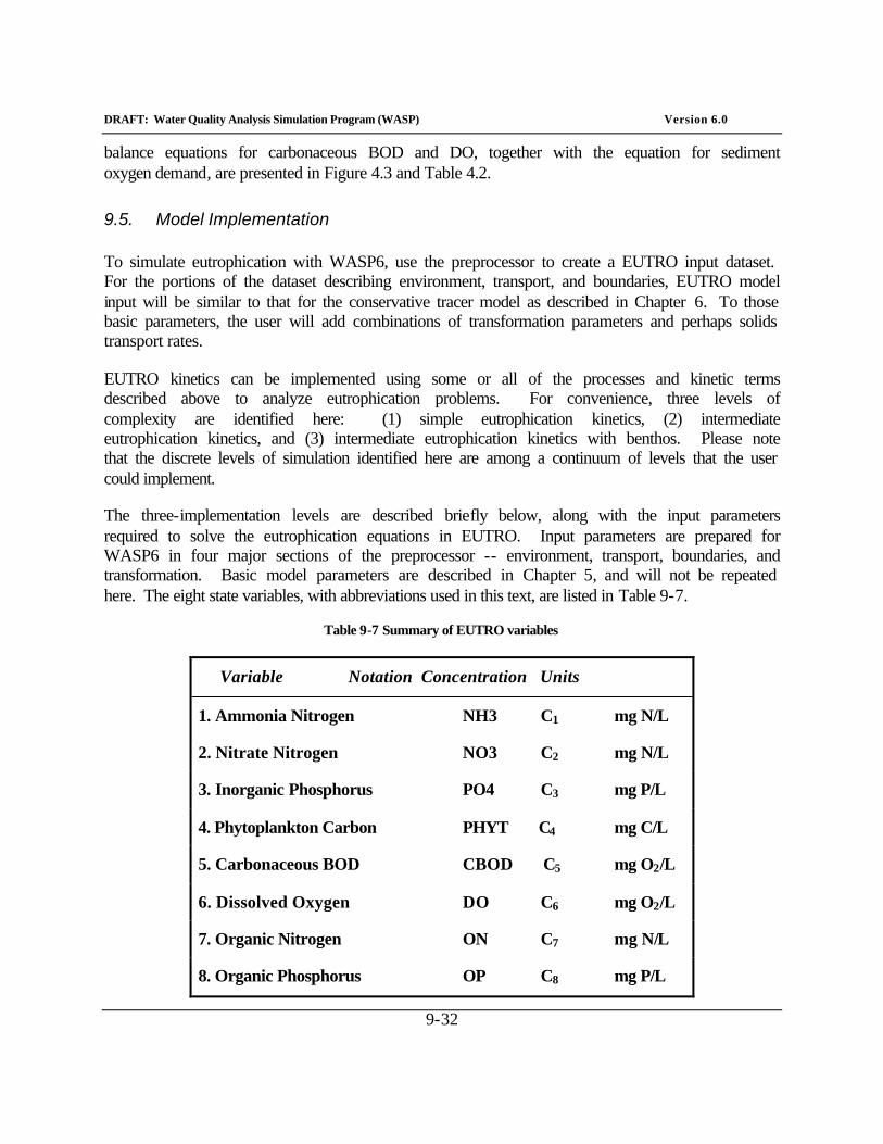
DRAFT: Water Quality Analysis Simulation Program (WASP) Version 6.0
9-32
balance equations for carbonaceous BOD and DO, together with the equation for sediment oxygen demand, are presented in Figure 4.3 and Table 4.2.
9.5. Model Implementation
To simulate eutrophication with WASP6, use the preprocessor to create a EUTRO input dataset. For the portions of the dataset describing environment, transport, and boundaries, EUTRO model input will be similar to that for the conservative tracer model as described in Chapter 6. To those basic parameters, the user will add combinations of transformation parameters and perhaps solids transport rates.
EUTRO kinetics can be implemented using some or all of the processes and kinetic terms described above to analyze eutrophication problems. For convenience, three levels of complexity are identified here: (1) simple eutrophication kinetics, (2) intermediate eutrophication kinetics, and (3) intermediate eutrophication kinetics with benthos. Please note that the discrete levels of simulation identified here are among a continuum of levels that the user could implement.
The three-implementation levels are described briefly below, along with the input parameters required to solve the eutrophication equations in EUTRO. Input parameters are prepared for WASP6 in four major sections of the preprocessor -- environment, transport, boundaries, and transformation. Basic model parameters are described in Chapter 5, and will not be repeated here. The eight state variables, with abbreviations used in this text, are listed in Table 9-7.
Table 9-7 Summary of EUTRO variables
Variable Notation Concentration Units
1. Ammonia Nitrogen NH3 C1 mg N/L
2. Nitrate Nitrogen NO3 C2 mg N/L
3. Inorganic Phosphorus PO4 C3 mg P/L
4. Phytoplankton Carbon PHYT C4 mg C/L
5. Carbonaceous BOD CBOD C5 mg O2/L
6. Dissolved Oxygen DO C6 mg O2/L
7. Organic Nitrogen ON C7 mg N/L
8. Organic Phosphorus OP C8 mg P/L
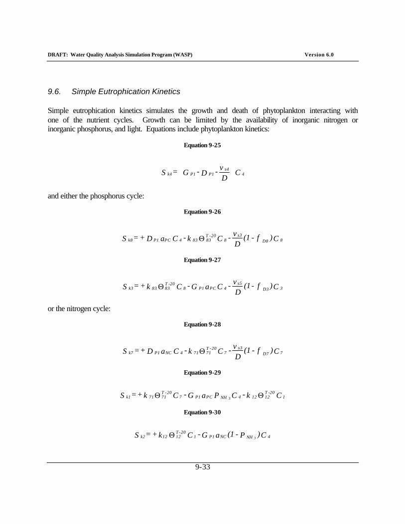
DRAFT: Water Quality Analysis Simulation Program (WASP) Version 6.0
9-33
9.6. Simple Eutrophication Kinetics
Simple eutrophication kinetics simulates the growth and death of phytoplankton interacting with one of the nutrient cycles. Growth can be limited by the availability of inorganic nitrogen or inorganic phosphorus, and light. Equations include phytoplankton kinetics:
Equation 9-25
C Dv - D - G = S 4
s4P1 P1 k4
and either the phosphorus cycle:
Equation 9-26
C )f - (1 Dv - C k - C a D + = S 8 D8
s38
20-T 83 83 4 PCP1 k8 Θ
Equation 9-27
C )f - (1 Dv - C a G - C k + = S 3 D3
s54 PCP1 8
20-T 83 83 k3 Θ
or the nitrogen cycle:
Equation 9-28
C )f - (1 Dv - C k - C a D + = S 7 D7
s37
20-T 71 71 4 NCP1 k7 Θ
Equation 9-29
C k -C P a G - C k + = S 1 20-T
12 12 4 NH PCP1 7 20-T
71 71 k1 3 ΘΘ
Equation 9-30
C )P - (1 a G - C k + = S 4 NH NCP1 1 20-T
12 12k2 3 Θ
DRAFT: Water Quality Analysis Simulation Program (WASP) Version 6.0
9-34
where Ski is the source/sink term for variable "i" in a segment, in mg/L-day. Kinetic rate constants and coefficients are as defined in Table 9-5, Table 9-4 and Table 9-3.
Phytoplankton plus either three nitrogen variables or two phosphorus variables are used in simple eutrophication simulations. While phytoplankton is simulated internally as mg/L carbon, initial concentrations and boundary concentrations are input by the user as µg/L chlorophyll a. EUTRO converts these input concentrations to internal concentrations using a user-specified carbon to chlorophyll ratio. If the carbon to chlorophyll ratio is not input, then a default value of 30 is used. Internal concentrations of phytoplankton nitrogen and phytoplankton phosphorus are calculated from user-specified nitrogen to carbon and phosphorus to carbon ratios. If these ratios are not input, then default values of 0.25 and 0.025 are used.
Simple eutrophication kinetics assumes that death returns phytoplankton nitrogen and phosphorus entirely to the organic nitrogen and organic phosphorus pools. Mineralization is a simple first order function that is unaffected by phytoplankton levels, and nitrification is a simple first order function unaffected by dissolved oxygen. Denitrification is not simulated.
Light limitation is described by the Di Toro formulation, Equation 9-4, and the user must calibrate the saturating light intensity Is.
The particulate fractions of ON and OP are associated with transport field 3, organic matter settling. Particulate PHYT is associated with transport field 4. The particulate fraction of PO4 is associated with transport field 5, inorganic settling.
9.6.1. Environment Parameters
These parameters define the basic model identity, including the segmentation, and control the simulation.
Systems-- Select "simulate" for PHYT and either ON, NH3, and NO3, or OP and PO4. Select "constant" for the nonsimulated nutrients and "bypass" for CBOD and DO. During calibration, the user may select "constant" or "bypass" for any selected variables.
Segments-- Water column segments should be defined in the standard fashion. If settling is to be simulated (i.e., for ON, OP, PHYT, or PO4), the user should add a single benthic segment underlying all water column segments. This benthic segment will merely act as a convenient sink for settling organic matter. Model calculations within this benthic segment should be ignored.
9.6.2. Transport Parameters
This group of parameters defines the advective and dispersive transport of model variables.
DRAFT: Water Quality Analysis Simulation Program (WASP) Version 6.0
9-35
Number of Flow Fields-- To simulate settling of ON and OP, the user should select solids 1 flow under advection. To simulate settling of PHYT, the user should select solids 2 flow. To simulate PO4 settling, the user should select solids 3 flow. The user should also select water column flow.
Particulate Transport, m3/sec-- Time variable settling and resuspension rates for solids 1, solids 2, and solids 3 can be input using the continuity array BQ and the time function QT. For each solids flow field, cross-sectional exchange areas (m2) for adjacent segment pairs are input using the spatially-variable BQ. Time-variable settling velocities can be specified as a series of velocities, in m/sec, versus time. If the units conversion factor is set to 1.157e-5, then these velocities are input in units of m/day. These velocities are multiplied internally by cross-sectional areas and treated as flows that carry particulate organic matter out of the water column.
9.6.3. Boundary Parameters
This group of parameters includes boundary concentrations, waste loads, and initial conditions. Boundary concentrations must be specified for any segment receiving flow inputs, outputs, or exchanges. Initial conditions include not only initial concentrations, but also the density and solids transport field for each solid, and the dissolved fraction in each segment.
Boundary Concentrations, mg/L-- At each segment boundary, time variable concentrations must be specified for PHYT, expressed as µg/L chlorophyll a. Time variable concentrations must also be specified for either ON, NH3, and NO3, or OP and PO4. A boundary segment is characterized by water exchanges from outside the network, including tributary inflows, downstream outflows, and open water dispersive exchanges.
Waste Loads, kg/day-- For each point source discharge, time variable PHYT, ON, NH3, NO3, OP, and PO4 loads can be specified. These loads can represent municipal and industrial wastewater discharges, or urban and agricultural runoff. If any phytoplankton loads are specified, they should be in units of kg carbon/day.
Solids Transport Field-- The transport fields associated with particulate settling must be specified under initial conditions. Solids 1 (Field 3) is recommended for ON and OP. Solids 2 (Field 4) is recommended for PHYT. Solids 3 (Field 5) is recommended for PO4.
Solid Density, g/cm3-- A value of 0 can be entered for the nominal density of PHYT, ON, NH3, NO3, OP, and PO4. This information is not used in EUTRO.
Initial Concentrations, mg/L-- Concentrations of PHYT, expressed as µg/L chlorophyll a and either ON, NH3, and NO3, or OP and PO4 in each segment must be specified for the time at which the simulation begins. For the nonsimulated nutrients held constant, average concentrations must be specified. These nutrient concentrations will remain constant throughout the simulation and can affect PHYT through growth rate limitation (although nonsimulated
DRAFT: Water Quality Analysis Simulation Program (WASP) Version 6.0
9-36
nutrients should be in excess and therefore not affect growth). Concentrations of zero for bypassed variables -- CBOD and DO -- will be entered by the preprocessor.
Dissolved Fraction-- The dissolved fraction of PHYT, ON, NH3, NO3, OP, and PO4 in each segment must be specified. The dissolved fraction of PHYT should be set to 0. Only the particulate fractions of the nutrients will be subject to settling.
9.6.4. Transformation Parameters
This group of parameters includes spatially variable parameters, constants, and kinetic time functions for the water quality constituents being simulated. Parameter values are entered for each segment. Specified values for constants apply over the entire network for the whole simulation. Kinetic time functions are composed of a series of values versus time, in days.
Water Temperature, C-- Time and segment variable water temperatures can be specified using the parameters TMPSG and TMPFN, and the time functions TEMP(1-4). If temperatures are to remain constant in time, then the user should enter segment temperatures using the parameter TMPSG. TMPFN and TEMP(1-4) should be omitted.
If the user wants to enter time-variable temperatures, then values for the parameter TMPSG should be set to 1.0. The parameter TMPFN indicates which temperature function will be used by the model for each segment. Values of 1.0, 2.0, 3.0, or 4.0 will call time functions TEMP(1), TEMP(2), TEMP(3), and TEMP(4), respectively. Water temperatures should then be entered via these time functions as a series of temperature versus time values. The product of TMPSG and the selected TEMP function will give the segment and time specific water temperatures used by EUTRO.
TMPSG and TMPFN are identified in EUTRO as parameters 3 and 4, respectively. TEMP(1-4) are identified in EUTRO as time functions 1-4.
Solar Radiation, langleys/day-- Time-variable solar radiation at the water surface can be described using time functions ITOT and FDAY. Seasonally-varying values of solar radiation at the surface can be entered using ITOT with a series of radiation versus time values. FDAY gives the seasonally-varying fraction of day that is daylight, entered as a series of fraction versus time values. Internally, EUTRO uses the quotient ITOT/FDAY for the average radiation intensity during daylight hours.
Light Extinction, m-1-- Time and segment variable light extinction coefficients can be specified using the parameters KESG and KEFN, and the time functions KE(1-5). If extinction coefficients are to remain constant in time, then the user should enter segment coefficients using the parameter KESG. KEFN and KE(1-4) should be omitted.
DRAFT: Water Quality Analysis Simulation Program (WASP) Version 6.0
9-37
If the user wants to enter time-variable extinction coefficients, then values for the parameter KESG should be set to 1.0. The parameter KEFN indicates which light extinction function will be used by the model for each segment. Values of 1.0, 2.0, 3.0, 4.0, or 5.0 will call time functions KE(1), KE(2), KE(3), KE(4), and KE(5), respectively. Light extinction coefficients should then be entered via these time functions as a series of coefficient versus time values. The product of KESG and the selected KE function will give the segment and time specific light extinction coefficients used by EUTRO.
KESG and KEFN are identified in EUTRO as parameters 5 and 6, respectively. KE(1-4) are identified in EUTRO as time functions 8-12.
Growth Rate, day-1-- The maximum phytoplankton growth rate constant and temperature coefficient can be input using constants K1C and K1T, respectively.
Carbon to Chlorophyll Ratio, mg C/mg Chl-- The average carbon to chlorophyll weight ratio in phytoplankton can be specified using constant CCHL. A default value of 30 is provided for in EUTRO.
Light Limitation-- Available light is specified using time functions describing seasonal light at the water surface and segment- and time-variable light extinction coefficients. These are described above.
The Di Toro light limitation option can be specified using a value of 1.0 for LGHTS. The saturating light intensity can then be specified using constant IS1. Default values for LGHTS and IS1 are 1 and 300, respectively.
Respiration Rate, day-1-- The average phytoplankton respiration rate constant and temperature coefficient can be input-using constants K1RC and K1RT, respectively.
Death Rate, day-1-- The non-predatory phytoplankton death rate constant can be input using constant K1D. No temperature dependence is assumed.
Phosphorus to Carbon Ratio, mg P/mg C-- The average phosphorus to carbon weight ratio in phytoplankton can be specified using constant PCRB. The EUTRO default value for PCRB is 0.025.
Phosphorus Mineralization Rate, day-1-- The mineralization rate constant and temperature coefficient for dissolved organic phosphorus can be specified using constants K83C and K83T, respectively.
Phosphorus Half-Saturation Constant, mg P/L-- The phosphorus half-saturation constant for phytoplankton growth can be specified using constant KMPG1. When inorganic phosphorus concentrations are at this level, the phytoplankton growth rate is reduced by half.
DRAFT: Water Quality Analysis Simulation Program (WASP) Version 6.0
9-38
Nitrogen to Carbon Ratio, mg N/mg C-- The average nitrogen to carbon weight ratio in phytoplankton can be specified using constant NCRB. The EUTRO default value for NCRB is 0.25.
Nitrogen Mineralization Rate, day-1-- The mineralization rate constant and temperature coefficient for dissolved organic nitrogen can be specified using constants K71C and K71T, respectively.
Nitrification Rate, day-1-- The nitrification rate constant and temperature coefficient for dissolved ammonia nitrogen can be specified using constants K12C and K12T, respectively.
Nitrogen Half-Saturation Constant, mg N/L-- The nitrogen half-saturation constant for phytoplankton growth can be specified using constant KMNG1. When inorganic nitrogen concentrations are at this level, the phytoplankton growth rate is reduced by half. This parameter also affects ammonia preference PNH3 as outlined in Figures 5.5 and 5.6. When KMNG1 = 0, PNH3 = 1.0. When KMNG1 becomes very large, PNH3 approaches a value of C1/(C1 + C2).
9.7. Intermediate Eutrophication Kinetics
Intermediate eutrophication kinetics simulates the growth and death of phytoplankton interacting with the nitrogen and phosphorus cycles and the dissolved oxygen balance. Growth can be limited by the availability of inorganic nitrogen, inorganic phosphorus, and light.
Intermediate eutrophication kinetics adds CBOD and DO equations as well as certain nonlinear terms and functions to the simple eutrophication kinetics described above. The oxygen balance equations and kinetic parameters are summarized in Figure 8-2 and Table 8-1. The phosphorus cycle equations and kinetic parameters are summarized in Figure 9-4 and Table 9-4. The nitrogen cycle equations and parameters are summarized in Figure 9-5 and Table 9-5. Phytoplankton equations are presented throughout Section 9.1.4, with parameters summarized in Table 9-2.
Either the Di Toro or the Smith formulation can describe light limitation. The Smith formulation implements equations Equation 9-5 through Equation 9-7. These equations predict the carbon to chlorophyll ratio based on the availability of light, and then predict the saturating light intensity based on the carbon to chlorophyll ratio.
Other terms included in the intermediate kinetics equations are the phytoplankton effect on mineralization of organic phosphorus and nitrogen, the dissolved oxygen limitation on nitrification, the denitrification reaction, and zooplankton grazing. The nonlinear DO balance equations can become important in inhibiting nitrification and carbonaceous oxidation and in promoting denitrification where low DO concentrations occur.
DRAFT: Water Quality Analysis Simulation Program (WASP) Version 6.0
9-39
All eight state variables are simulated in intermediate eutrophication simulations. During calibration of the model to observed data, however, the user may want to bypass certain variables or hold them constant. Nutrients can be held at observed concentrations, for instance, while phytoplankton growth and death rates are calibrated.
9.7.1. Environment Parameters
These parameters define the basic model identity, including the segmentation, and control the simulation.
Systems-- Select "simulate" for all variables. During calibration, the user may select "constant" or "bypass" for any selected variables.
Segments-- Water column segments should be defined in the standard fashion. If settling is to be simulated (i.e., for ON, OP, PHYT, PO4, or CBOD), the user should add a single benthic segment underlying all water column segments. This benthic segment will merely act as a convenient sink for settling organic matter. Model calculations within this benthic segment should be ignored.
9.7.2. Transport Parameters
This group of parameters defines the advective and dispersive transport of model variables.
Number of Flow Fields-- To simulate settling of ON, OP, and CBOD, the user should select solids 1 flow under advection. To simulate settling of PHYT, the user should select solids 2 flow. To simulate PO4 settling, the user should select solids 3 flow. The user should also select water column flow.
Particulate Transport, m3/sec-- Time variable settling and resuspension velocities can be specified for particulate ON, OP, CBOD, PHYT, and PO4, as described in the simple eutrophication section above.
9.7.3. Boundary Parameters
This group of parameters includes boundary concentrations, waste loads, and initial conditions. Boundary concentrations must be specified for any segment receiving flow inputs, outputs, or exchanges. Initial conditions include not only initial concentrations, but also the density and solids transport field for each solid, and the dissolved fraction in each segment.
Boundary Concentrations, mg/L-- At each segment boundary, time variable concentrations must be specified for PHYT, expressed as µg/L chlorophyll a. Time variable concentrations must also be specified for either ON, NH3, NO3, OP, PO4, CBOD, and DO. A boundary segment is
DRAFT: Water Quality Analysis Simulation Program (WASP) Version 6.0
9-40
characterized by water exchanges from outside the network, including tributary inflows, downstream outflows, and open water dispersive exchanges.
Waste Loads, kg/day-- For each point source discharge, time variable PHYT, ON, NH3, NO3, OP, PO4, CBOD, and DO loads can be specified. These loads can represent municipal and industrial wastewater discharges, or urban and agricultural runoff. If any phytoplankton loads are specified, they should be in units of kg carbon/day.
Solids Transport Field-- The transport fields associated with particulate settling must be specified under initial conditions. Solids 1 (Field 3) is recommended for ON, OP, and CBOD. Solids 2 (Field 4) is recommended for PHYT. Solids 3 (Field 5) is recommended for PO4.
Solid Density, g/cm3-- A value of 0 can be entered for the nominal density of PHYT, ON, NH3, NO3, OP, PO4, CBOD, and DO. This information is not used in EUTRO.
Initial Concentrations, mg/L-- Concentrations of all variables in each segment must be specified for the time at which the simulation begins. Concentrations of PHYT are expressed as µg/L chlorophyll a.
Dissolved Fraction-- The dissolved fraction of each variable in each segment must be specified. The dissolved fraction of PHYT should be set to 0, and the dissolved fraction of DO should be set to 1. Only the particulate fractions of CBOD and the nutrients will be subject to settling.
9.7.4. Transformation Parameters
This group of parameters includes spatially variable parameters, constants, and kinetic time functions for the water quality constituents being simulated. Parameter values are entered for each segment. Specified values for constants apply over the entire network for the whole simulation. Kinetic time functions are composed of a series of values versus time, in days.
Water Temperature, C-- Time and segment variable water temperatures can be specified using the parameters TMPSG and TMPFN, and the time functions TEMP(1-4), as described in the simple eutrophication section above.
Solar Radiation, langleys/day-- Time-variable solar radiation at the water surface can be described using time functions ITOT and FDAY, as described in the simple eutrophication section above.
Light Extinction, m-1-- Time and segment variable light extinction coefficients can be specified using the parameters KESG and KEFN, and the time functions KE(1-5), as described in the simple eutrophication section above.
DRAFT: Water Quality Analysis Simulation Program (WASP) Version 6.0
9-41
Growth Rate, day-1-- The maximum phytoplankton growth rate constant and temperature coefficient can be input using constants K1C and K1T, respectively.
Carbon to Chlorophyll Ratio, mg C/mg Chl-- The average carbon to chlorophyll weight ratio in phytoplankton can be specified using constant CCHL. A default value of 30 is provided for in EUTRO. If the Smith light limitation option is chosen, then CCHL will be variable, recalculated daily throughout the simulation.
Light Limitation-- Available light is specified using time functions describing seasonal light at the water surface and segment- and time-variable light extinction coefficients. These are described above.
The Di Toro light limitation option can be specified using a value of 1.0 for LGHTS. The saturating light intensity, in langleys/day can then be specified using constant IS1. Default values for LGHTS and IS1 are 1 and 300, respectively.
The Smith light limitation option can be specified using a value of 2.0 for LGHTS. Two other parameters must then be specified. The maximum quantum yield constant, in mg C/mole photons, can be specified using constant PHIMX. The chlorophyll extinction coefficient, in (mg chl a/m3)-1m-1, can be specified using constant XKC. Default values for PHIMX and XKC are 720 and 0.017, respectively.
Nitrogen Half-Saturation Constant, mg N/L-- The nitrogen half-saturation constant for phytoplankton growth can be specified using constant KMNG1. When inorganic nitrogen concentrations are at this level, half reduces the phytoplankton growth rate. This parameter also affects ammonia preference PNH3 as outlined in Figures 5.5 and 5.6. When KMNG1 = 0, PNH3 = 1.0. When KMNG1 becomes very large, PNH3 approaches a value of C1/(C1 + C2).
Phosphorus Half-Saturation Constant, mg P/L-- The phosphorus half-saturation constant for phytoplankton growth can be specified using constant KMPG1. When inorganic phosphorus concentrations are at this level, half reduces the phytoplankton growth rate.
Nutrient Limitation Option-- The nutrient limitation formulation can be specified using constant NUTLIM. A value of 0 selects the minimum formulation, which is recommended. A value of 1.0 selects the multiplicative formulation. The default value is 0.
Respiration Rate, day-1-- The average phytoplankton endogenous respiration rate constant and temperature coefficient can be input-using constants K1RC and K1RT, respectively.
Death Rate, day-1-- The non-predatory phytoplankton death rate constant can be input using constant K1D. No temperature dependance is assumed.
Grazing Rate, day-1-- Zooplankton grazing can be specified using parameter ZOOSG, time function ZOO, and constant K1G. Time- and segment-variable herbivorous zooplankton

DRAFT: Water Quality Analysis Simulation Program (WASP) Version 6.0
9-42
populations are described as the product of the time variable population ZOO, in mg zooplankton C/L, and segment specific ratios ZOOSG. The grazing rate per unit zooplankton population, in L/mg zooplankton C-day, can be input using constant K1G. The resulting grazing rate constant for phytoplankton is the product of the variable zooplankton population and the unit grazing rate. (Note that ZOO can also be expressed as cells/L if K1G is expressed as L/cell-day).
Phosphorus to Carbon Ratio, mg P/mg C-- The average phosphorus to carbon weight ratio in phytoplankton can be specified using constant PCRB. The EUTRO default value for PCRB is 0.025.
Phytoplankton Phosphorus Recycle-- The fraction of dead and respired phytoplankton phosphorus that is recycled to the organic phosphorus pool can be specified using constant FOP. The default value is 1. The fraction of phytoplankton phosphorus recycled directly to inorganic phosphorus is 1 - FOP.
Phosphorus Mineralization Rate, day-1-- The mineralization rate constant and temperature coefficient for dissolved organic phosphorus can be specified using constants K83C and K83T, respectively. Phytoplankton effects on mineralization can be described using constant KMPHY, the half-saturation constant for mineralization dependence on phytoplankton, in mg C/L. This causes mineralization rates to increase as phytoplankton levels increase. If KMPHY is zero, there is no phytoplankton effect on mineralization. If KMPHY is large, then large concentrations of phytoplankton are needed to drive mineralization, and thus relatively low phytoplankton levels can lead to low mineralization rates.
Benthic Phosphorus Flux, mg/m2-day-- The segment- and time-variable benthic phosphorus flux can be specified using parameter FPO4 and time function TFPO4. The product of the spatially- variable FPO4 and time-variable TFPO4 gives the segment and time specific benthic flux for PO4 used by EUTRO. Flux versus time values can be entered using TFPO4, while unitless segment ratios can be entered using FPO4. Values should be entered for water column segments that are in contact with the bottom of the water body.
Nitrogen to Carbon Ratio, mg N/mg C-- The average nitrogen to carbon weight ratio in phytoplankton can be specified using constant NCRB. The EUTRO default value for NCRB is 0.25.
Phytoplankton Nitrogen Recycle-- The fraction of dead and respired phytoplankton nitrogen that is recycled to the organic nitrogen pool can be specified using constant FON. The default value is 1. The fraction of phytoplankton nitrogen recycled directly to ammonia is 1 - FON.
Nitrogen Mineralization Rate, day-1-- The mineralization rate constant and temperature coefficient for dissolved organic nitrogen can be specified using constants K71C and K71T, respectively. Phytoplankton effects on mineralization can be described using constant KMPHY,

DRAFT: Water Quality Analysis Simulation Program (WASP) Version 6.0
9-43
the half-saturation constant for mineralization dependence on phytoplankton, as explained above in the phosphorus mineralization section.
Nitrification Rate, day-1-- The nitrification rate constant and temperature coefficient for dissolved ammonia nitrogen can be specified using constants K12C and K12T, respectively. The half-saturation constant for oxygen limitation of nitrification can be specified using constant KNIT. The default value for KNIT is 0.0, indicating no oxygen limitation.
Denitrification Rate, day-1-- The denitrification rate constant and temperature coefficient for dissolved nitrate nitrogen can be specified using constants K20C and K20T, respectively. The half-saturation constant for oxygen limitation of denitrification can be specified using constant KNO3. The default value for KNO3 is 0.0, indicating no denitrification at oxygen concentrations above 0.0.
Benthic Nitrogen Flux, mg/m2-day-- The segment- and time-variable benthic nitrogen flux can be specified using parameter FNH4 and time function TFNH4. The product of the spatially- variable FNH4 and time-variable TFNH4 gives the segment and time specific benthic flux for NH3 used by EUTRO. Flux versus time values can be entered using TFNH4, while unitless segment ratios can be entered using FNH4. Values should be entered for water column segments that are in contact with the bottom of the water body.
Sediment Oxygen Demand, g/m2-day-- Segment variable sediment oxygen demand fluxes and temperature coefficients can be specified using the parameters SOD1D and SODTA, respectively. Values should be entered for water column segments that are in contact with the bottom of the water body.
Reaeration Rate, day-1-- There are three basic options for specifying reaeration -- a single rate constant, segment and time variable rate constants, and flow and wind calculated rate constants. These options are described in Section 4.2, under the Streeter-Phelps transformation parameters.
CBOD Deoxygenation Rate, day-1-- The CBOD deoxygenation rate constant and temperature coefficient can be specified using constants KDC and KDT, respectively. The half-saturation constant for oxygen limitation of carbonaceous deoxygenation can be specified using constant KBOD. The default value for KBOD is 0.0, indicating no oxygen limitation.
9.8. Intermediate Eutrophication Kinetics with Benthos
Simulating benthic interactions requires the addition of benthic segments to the model network. All state variables are simulated in the benthic segments. Dissolved fractions of NH3, NO3, PO4, CBOD, DO, ON, and OP may exchange with the water column by diffusion. Particulate fractions of PHYT, PO4, CBOD, ON, and OP may deposit to or be scoured from the benthic segments. Benthic layer decomposition rates for OP, ON, PHYT, and CBOD must be specified.
DRAFT: Water Quality Analysis Simulation Program (WASP) Version 6.0
9-44
The equations used are those presented in Figure 8-4 and Figure 9-8. Rate parameters are summarized in Table 8-2 and Table 9-6.
Many of the environment, transport, boundary, and transformation parameters required to implement this option are the same as those in the intermediate eutrophication option presented above. The benthic nitrogen and phosphorus flux functions should be omitted, and the following should be modified or added.
Segments-- Water column segments should be defined in the standard fashion. In addition, the user should add a benthic segment underlying each water column segment (or stack of water column segments). These benthic segments will receive settling organic and inorganic matter from the water column above, and can return material to the water column via resuspension or by pore water diffusion.
Phytoplankton Decomposition, day-1-- The user may specify the rate constant and temperature coefficient for phytoplankton decomposition in benthic segments using constants KPZDC and KPZDT.
Carbonaceous BOD Decomposition, day-1-- The user may specify the rate constant and temperature coefficient for CBOD decomposition in benthic segments using constants KDSC and KDST.
Organic Nitrogen Decomposition, day-1-- The user may specify the rate constant and temperature coefficient for organic nitrogen decomposition in benthic segments using constants KONDC and KONDT.
Organic Phosphorus Decomposition, day-1-- The user may specify the rate constant and temperature coefficient for organic phosphorus decomposition in benthic segments using constants KOPDC and KOPDT.
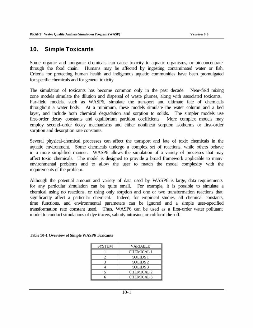
DRAFT: Water Quality Analysis Simulation Program (WASP) Version 6.0
10-1
10. Simple Toxicants
Some organic and inorganic chemicals can cause toxicity to aquatic organisms, or bioconcentrate through the food chain. Humans may be affected by ingesting contaminated water or fish. Criteria for protecting human health and indigenous aquatic communities have been promulgated for specific chemicals and for general toxicity.
The simulation of toxicants has become common only in the past decade. Near-field mixing zone models simulate the dilution and dispersal of waste plumes, along with associated toxicants. Far-field models, such as WASP6, simulate the transport and ultimate fate of chemicals throughout a water body. At a minimum, these models simulate the water column and a bed layer, and include both chemical degradation and sorption to solids. The simpler models use first-order decay constants and equilibrium partition coefficients. More complex models may employ second-order decay mechanisms and either nonlinear sorption isotherms or first-order sorption and desorption rate constants.
Several physical-chemical processes can affect the transport and fate of toxic chemicals in the aquatic environment. Some chemicals undergo a complex set of reactions, while others behave in a more simplified manner. WASP6 allows the simulation of a variety of processes that may affect toxic chemicals. The model is designed to provide a broad framework applicable to many environmental problems and to allow the user to match the model complexity with the requirements of the problem.
Although the potential amount and variety of data used by WASP6 is large, data requirements for any particular simulation can be quite small. For example, it is possible to simulate a chemical using no reactions, or using only sorption and one or two transformation reactions that significantly affect a particular chemical. Indeed, for empirical studies, all chemical constants, time functions, and environmental parameters can be ignored and a simple user-specified transformation rate constant used. Thus, WASP6 can be used as a first-order water pollutant model to conduct simulations of dye tracers, salinity intrusion, or coliform die-off.
Table 10-1 Overview of Simple WASP6 Toxicants
SYSTEM VARIABLE 1 CHEMICAL 1 2 SOLIDS 1 3 SOLIDS 2 4 SOLIDS 3 5 CHEMICAL 2 6 CHEMICAL 3
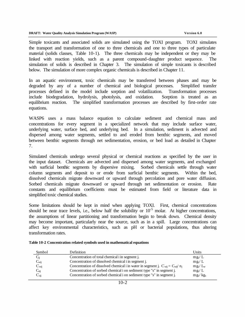
DRAFT: Water Quality Analysis Simulation Program (WASP) Version 6.0
10-2
Simple toxicants and associated solids are simulated using the TOXI program. TOXI simulates the transport and transformation of one to three chemicals and one to three types of particulate material (solids classes, Table 10-1). The three chemicals may be independent or they may be linked with reaction yields, such as a parent compound-daughter product sequence. The simulation of solids is described in Chapter 3. The simulation of simple toxicants is described below. The simulation of more complex organic chemicals is described in Chapter 11.
In an aquatic environment, toxic chemicals may be transferred between phases and may be degraded by any of a number of chemical and biological processes. Simplified transfer processes defined in the model include sorption and volatilization. Transformation processes include biodegradation, hydrolysis, photolysis, and oxidation. Sorption is treated as an equilibrium reaction. The simplified transformation processes are described by first-order rate equations.
WASP6 uses a mass balance equation to calculate sediment and chemical mass and concentrations for every segment in a specialized network that may include surface water, underlying water, surface bed, and underlying bed. In a simulation, sediment is advected and dispersed among water segments, settled to and eroded from benthic segments, and moved between benthic segments through net sedimentation, erosion, or bed load as detailed in Chapter 7.
Simulated chemicals undergo several physical or chemical reactions as specified by the user in the input dataset. Chemicals are advected and dispersed among water segments, and exchanged with surficial benthic segments by dispersive mixing. Sorbed chemicals settle through water column segments and deposit to or erode from surficial benthic segments. Within the bed, dissolved chemicals migrate downward or upward through percolation and pore water diffusion. Sorbed chemicals migrate downward or upward through net sedimentation or erosion. Rate constants and equilibrium coefficients must be estimated from field or literature data in simplified toxic chemical studies.
Some limitations should be kept in mind when applying TOXI. First, chemical concentrations should be near trace levels, i.e., below half the solubility or 10-5 molar. At higher concentrations, the assumptions of linear partitioning and transformation begin to break down. Chemical density may become important, particularly near the source, such as in a spill. Large concentrations can affect key environmental characteristics, such as pH or bacterial populations, thus altering transformation rates.
Table 10-2 Concentration related symbols used in mathematical equations
Symbol Definition Units Cij Concentration of total chemical i in segment j. mgc/L Cwij Concentration of dissolved chemical i in segment j. mgc/L C'wij Concentration of dissolved chemical i in water in segment j. C'wij = Cwij/nj mgc/Lw Csij Concentration of sorbed chemical i on sediment type "s" in segment j. mgc/L C'sij Concentration of sorbed chemical i on sediment type "s" in segment j. mgc/kgs
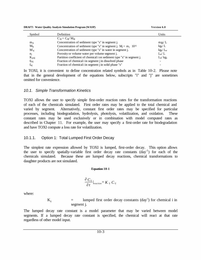
DRAFT: Water Quality Analysis Simulation Program (WASP) Version 6.0
10-3
Symbol Definition Units C'sij = Csij/Msij
msj Concentration of sediment type "s" in segment j. mgs/L Msj Concentration of sediment type "s" in segment j. Mj = m j ⋅ 10-6 kgs/L M'sj Concentration of sediment type "s" in water in segment j. kgs/Lw nj Porosity or volume water per volume segment j. Lw/L Kpsij Partition coefficient of chemical i on sediment type "s" in segment j. Lw/kgs fDij Fraction of chemical i in segment j in dissolved phase - fsij Fraction of chemical i in segment j in solid phase "s" -
In TOXI, it is convenient to define concentration related symbols as in Table 10-2. Please note that in the general development of the equations below, subscripts "i" and "j" are sometimes omitted for convenience.
10.1. Simple Transformation Kinetics
TOXI allows the user to specify simple first-order reaction rates for the transformation reactions of each of the chemicals simulated. First order rates may be applied to the total chemical and varied by segment. Alternatively, constant first order rates may be specified for particular processes, including biodegradation, hydrolysis, photolysis, volatilization, and oxidation. These constant rates may be used exclusively or in combination with model computed rates as described in Chapter 11. For example, the user may specify a first-order rate for biodegradation and have TOXI compute a loss rate for volatilization.
10.1.1. Option 1: Total Lumped First Order Decay
The simplest rate expression allowed by TOXI is lumped, first-order decay. This option allows the user to specify spatially-variable first order decay rate constants (day-1) for each of the chemicals simulated. Because these are lumped decay reactions, chemical transformations to daughter products are not simulated.
Equation 10-1
C K = | t
C ij ij reaction
ij
∂∂
where:
Kij = lumped first order decay constants (day-1) for chemical i in segment j.
The lumped decay rate constant is a model parameter that may be varied between model segments. If a lumped decay rate constant is specified, the chemical will react at that rate regardless of other model input.
DRAFT: Water Quality Analysis Simulation Program (WASP) Version 6.0
10-4
10.1.2. Option 2: Individual First Order Transformation
This option allows the user to input a global first-order reaction rate constant separately for each of the following processes: volatilization, water column biodegradation, benthic biodegradation, alkaline hydrolysis, neutral hydrolysis, acid hydrolysis, oxidation, photolysis, and an extra reaction. The total reaction is then based on the sum of each of the individual reactions as given by
Equation 10-2
C K = | t
C ij ki
N
=1kreaction
ij ∑∂∂
where:
Kki = first order transformation constants for reaction k of chemical i, day-1
The user may input half-lives rather than first-order decay rate constants. If half-lives are provided for the transformation reactions, they will be converted internally to first order rate constants and used as above:
Equation 10-3
T/ 0.693 = K Hki ki
where:
THki = half-life of reaction k for chemical i, days.
10.2. Equilibrium Sorption
Sorption is the bonding of dissolved chemicals onto solid phases, such as benthic and suspended sediment, biological material, and sometime dissolved or colloidal organic material. Sorption can be important in controlling both the environmental fate and the toxicity of chemicals. Sorption may cause the chemical to accumulate in bed sediment or bioconcentrate in fish. Sorption may retard such reactions as volatilization and base hydrolysis, or enhance other reactions including photolysis and acid-catalyzed hydrolysis.
Sorption reactions are usually fast relative to other environmental processes, and equilibrium may be assumed. For environmentally relevant concentrations (less than 10-5 M or one-half water solubility), equilibrium sorption is linear with dissolved chemical concentration (Karickhoff, 1984) or:
DRAFT: Water Quality Analysis Simulation Program (WASP) Version 6.0
10-5
Equation 10-4
C K = C wpss ′′ •
At equilibrium, then, the distribution among the phases is controlled by the partition coefficients Kps. As developed in Chapter 7, the total mass of chemical in each phase is controlled by Kps and the amount of solid phase present (ignoring here any DOC phase), so that
Equation 10-5
M K + nn
= f sps
s
D •∑
and
Equation 10-6
M K + nM K = f
sps s
sps s •
•
∑
These fractions are determined in time and space throughout a simulation from the partition coefficients, internally calculated porosities, and simulated sediment concentrations. Given the total concentration and the phase fractions of chemical i in segment j, the dissolved and sorbed concentrations are uniquely determined:
Equation 10-7
f C = C Dij ij wij •
Equation 10-8
f C = C sijij sij •
In addition to the assumption of instantaneous equilibrium, implicit in the use of these equations is the assumption of reversibility. Laboratory data for very hydrophobic chemicals suggest, however, that a hysteresis exists, with desorption being a much slower process than adsorption. Karickhoff suggests that this effect may be the result of intraparticle kinetics in which the chemical is slowly incorporated into components of the sorbant. This phenomenon is not well understood and no quantitative modeling framework is available to characterize it.
DRAFT: Water Quality Analysis Simulation Program (WASP) Version 6.0
10-6
Values for the partition coefficients can be obtained from laboratory experiments or field data. TOXI allows the input of either a single constant partition coefficient, or a set of spatially-variable partition coefficients. These options are described under "Model Implementation" below. The calculation of partition coefficients for organic chemicals is described in Chapter 7.
10.3. Transformations and Daughter Products
The three chemicals that may be simulated by TOXI may be independent, or they may be linked with reaction yields, such as a parent compound-daughter product sequence. Linked transformations may be implemented by simulating two or three chemicals and by specifying appropriate yield coefficients for each process:
Equation 10-9
3 2, = c ,Y C K = S kc1 c kc kc
kc1 ∑∑
Equation 10-10
3 1, = c ,Y C K = S kc2 c kc kc
kc2 ∑∑
Equation 10-11
2 1, = c ,Y C K = S kc3 c kc kc
kc3 ∑∑
where:
Skci= production of chemical "i" from chemical "c" undergoing reaction "k," mgi/L-day
Kkc = effective rate coefficient for chemical "c," reaction "k," day-1 Ykci = yield coefficients for production of chemical "i" from
chemical "c" undergoing reaction "k," mgi/mgc
8 illustrates some of the linked reactions that can be simulated by specifying appropriate yield coefficients.
Potential reaction products in WASP
DRAFT: Water Quality Analysis Simulation Program (WASP) Version 6.0
10-7
10.4. Model Implementation
To simulate simple toxicants with WASP6, use the preprocessor to create a TOXI input file. The model input dataset and the input parameters will be similar to those for the conservative tracer model as described in Chapter 2. To those basic parameters, the user will add benthic segments; solids transport rates, and transformation parameters. During the simulation, solids and toxicants will be transported both by the water column advection and dispersion rates and by these solids transport rates.
In WASP6, solids transport rates in the water column and the bed are input via up to three solids transport fields, as described in Chapter 3. The transport of the particulate fraction of toxicants follows the solids flows. The user must specify the dissolved fraction (i.e. 0.0) and the solids transport field for each simulated solid under initial conditions. To simulate total solids, solids 1 must be used.
10.4.1. Model Input Parameters
This section summarizes the input parameters that must be specified in order to solve the simple toxicant equations in TOXI. The user is referred to Chapter 3 for a summary of input parameters for the sediment balance equations. Input parameters are prepared for WASP6 in four major sections of the preprocessor -- environment, transport, boundaries, and transformation. Basic model parameters are described in Chapter 2, and will not be repeated here.
10.4.2. Environment Parameters
These parameters define the basic model identity, including the segmentation, and control the simulation.
Systems-- To simulate a toxicant, select "simulate" for chemical 1 and "bypass" for chemical 2 and chemical 3. To simulate total solids along with the toxicant, select "simulate" for solids 1 and "bypass" for solids 2 and solids 3. To simulate two or more toxicants or solids, select "simulate" for the appropriate variable.
Bed Volume Option-- The user must determine whether bed volumes are to be held constant or allowed to vary. Volumes may be held constant by specifying 0, in which case sediment concentrations and porosities in the bed segments will vary. Alternatively, sediment concentrations and porosities may be held constant by specifying 1, in which case surficial bed segment volumes will vary.
Bed Time Step-- While mass transport calculations are repeated every model time step, certain benthic calculations are repeated only at this benthic time step, in days. If the constant bed volume option is chosen, sediment concentrations are updated every model time step, but
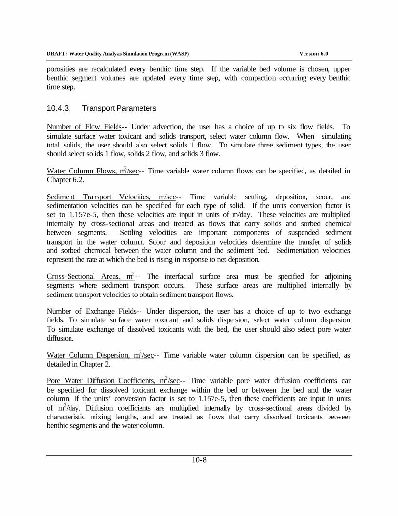
DRAFT: Water Quality Analysis Simulation Program (WASP) Version 6.0
10-8
porosities are recalculated every benthic time step. If the variable bed volume is chosen, upper benthic segment volumes are updated every time step, with compaction occurring every benthic time step.
10.4.3. Transport Parameters
Number of Flow Fields-- Under advection, the user has a choice of up to six flow fields. To simulate surface water toxicant and solids transport, select water column flow. When simulating total solids, the user should also select solids 1 flow. To simulate three sediment types, the user should select solids 1 flow, solids 2 flow, and solids 3 flow.
Water Column Flows, m3/sec-- Time variable water column flows can be specified, as detailed in Chapter 6.2.
Sediment Transport Velocities, m/sec-- Time variable settling, deposition, scour, and sedimentation velocities can be specified for each type of solid. If the units conversion factor is set to 1.157e-5, then these velocities are input in units of m/day. These velocities are multiplied internally by cross-sectional areas and treated as flows that carry solids and sorbed chemical between segments. Settling velocities are important components of suspended sediment transport in the water column. Scour and deposition velocities determine the transfer of solids and sorbed chemical between the water column and the sediment bed. Sedimentation velocities represent the rate at which the bed is rising in response to net deposition.
Cross-Sectional Areas, m2-- The interfacial surface area must be specified for adjoining segments where sediment transport occurs. These surface areas are multiplied internally by sediment transport velocities to obtain sediment transport flows.
Number of Exchange Fields-- Under dispersion, the user has a choice of up to two exchange fields. To simulate surface water toxicant and solids dispersion, select water column dispersion. To simulate exchange of dissolved toxicants with the bed, the user should also select pore water diffusion.
Water Column Dispersion, m3/sec-- Time variable water column dispersion can be specified, as detailed in Chapter 2.
Pore Water Diffusion Coefficients, m2/sec-- Time variable pore water diffusion coefficients can be specified for dissolved toxicant exchange within the bed or between the bed and the water column. If the units’ conversion factor is set to 1.157e-5, then these coefficients are input in units of m2/day. Diffusion coefficients are multiplied internally by cross-sectional areas divided by characteristic mixing lengths, and are treated as flows that carry dissolved toxicants between benthic segments and the water column.
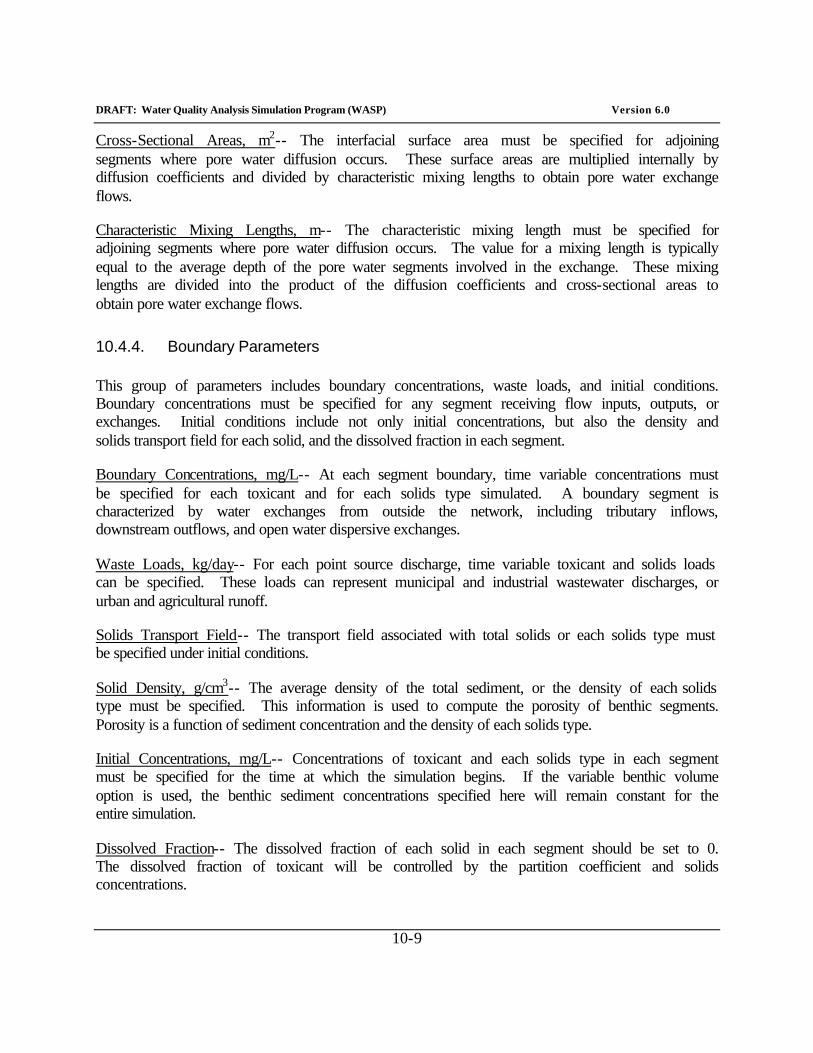
DRAFT: Water Quality Analysis Simulation Program (WASP) Version 6.0
10-9
Cross-Sectional Areas, m2-- The interfacial surface area must be specified for adjoining segments where pore water diffusion occurs. These surface areas are multiplied internally by diffusion coefficients and divided by characteristic mixing lengths to obtain pore water exchange flows.
Characteristic Mixing Lengths, m-- The characteristic mixing length must be specified for adjoining segments where pore water diffusion occurs. The value for a mixing length is typically equal to the average depth of the pore water segments involved in the exchange. These mixing lengths are divided into the product of the diffusion coefficients and cross-sectional areas to obtain pore water exchange flows.
10.4.4. Boundary Parameters
This group of parameters includes boundary concentrations, waste loads, and initial conditions. Boundary concentrations must be specified for any segment receiving flow inputs, outputs, or exchanges. Initial conditions include not only initial concentrations, but also the density and solids transport field for each solid, and the dissolved fraction in each segment.
Boundary Concentrations, mg/L-- At each segment boundary, time variable concentrations must be specified for each toxicant and for each solids type simulated. A boundary segment is characterized by water exchanges from outside the network, including tributary inflows, downstream outflows, and open water dispersive exchanges.
Waste Loads, kg/day-- For each point source discharge, time variable toxicant and solids loads can be specified. These loads can represent municipal and industrial wastewater discharges, or urban and agricultural runoff.
Solids Transport Field-- The transport field associated with total solids or each solids type must be specified under initial conditions.
Solid Density, g/cm3-- The average density of the total sediment, or the density of each solids type must be specified. This information is used to compute the porosity of benthic segments. Porosity is a function of sediment concentration and the density of each solids type.
Initial Concentrations, mg/L-- Concentrations of toxicant and each solids type in each segment must be specified for the time at which the simulation begins. If the variable benthic volume option is used, the benthic sediment concentrations specified here will remain constant for the entire simulation.
Dissolved Fraction-- The dissolved fraction of each solid in each segment should be set to 0. The dissolved fraction of toxicant will be controlled by the partition coefficient and solids concentrations.

DRAFT: Water Quality Analysis Simulation Program (WASP) Version 6.0
10-10
10.4.5. Transformation Parameters
This group of parameters includes spatially variable parameters, constants, and kinetic time functions for the water quality constituents being simulated. None are necessary for sediment transport.
First-Order Degradation-- There are two options to input first-order toxicant degradation:
Option 1: Total Lumped First Order Decay
The use of the simple lumped first-order decay rate requires the user to input a decay rate constant for the chemical for each model segment. If a simple lumped first order rate is specified for a particular chemical, the chemical will decay at that rate regardless of other input. For example, if both a lumped decay rate and either a simple first order or second order transformation rate are specified, the simple first or second order rates will only be used if the lumped rate is zero.
Option 2: Individual First Order Transformation
Constant C1 C2 C3 REACTION KV, day-1 140 740 1340 Volatilization THV, day 145? 745? 1345? KBW, day-1 141 741 1341 Water Column
Biodegradation THBW, day 143 743 1343 KBS, day-1 142 742 1342 Benthic
Biodegradation THBS, day 144 744 1344 KHOH, day-1 181 781 1381 Alkaline
Hydrolysis THHOH, day 252 852 1452 KHN, day-1 182 782 1382 Neutral
Hydrolysis THHN, day 253 853 1453 KHH, day-1 183 783 1383 Acid
Hydrolysis THHH, day 254 854 1454 KO, day-1 256 856 1456 Oxidation THO, day 257 857 1457 KF, day-1 287 887 1482 Photolysis THF, day 289 889 1489 KE, day-1 571 1171 1771 Extra Reaction THE, day 572 1172 1772
The use of the simple first-order transformation rate requires the user to input a global rate constant (day-1) or half-life (day) for each particular processes simulated. If a simple first-order
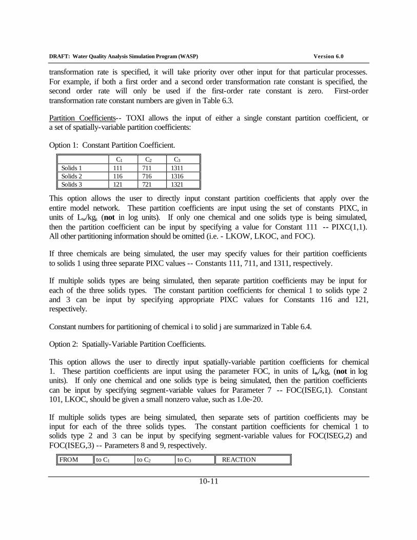
DRAFT: Water Quality Analysis Simulation Program (WASP) Version 6.0
10-11
transformation rate is specified, it will take priority over other input for that particular processes. For example, if both a first order and a second order transformation rate constant is specified, the second order rate will only be used if the first-order rate constant is zero. First-order transformation rate constant numbers are given in Table 6.3.
Partition Coefficients-- TOXI allows the input of either a single constant partition coefficient, or a set of spatially-variable partition coefficients:
Option 1: Constant Partition Coefficient.
C1 C2 C3 Solids 1 111 711 1311 Solids 2 116 716 1316 Solids 3 121 721 1321
This option allows the user to directly input constant partition coefficients that apply over the entire model network. These partition coefficients are input using the set of constants PIXC, in units of Lw/kgs (not in log units). If only one chemical and one solids type is being simulated, then the partition coefficient can be input by specifying a value for Constant 111 -- PIXC(1,1). All other partitioning information should be omitted (i.e. - LKOW, LKOC, and FOC).
If three chemicals are being simulated, the user may specify values for their partition coefficients to solids 1 using three separate PIXC values -- Constants 111, 711, and 1311, respectively.
If multiple solids types are being simulated, then separate partition coefficients may be input for each of the three solids types. The constant partition coefficients for chemical 1 to solids type 2 and 3 can be input by specifying appropriate PIXC values for Constants 116 and 121, respectively.
Constant numbers for partitioning of chemical i to solid j are summarized in Table 6.4.
Option 2: Spatially-Variable Partition Coefficients.
This option allows the user to directly input spatially-variable partition coefficients for chemical 1. These partition coefficients are input using the parameter FOC, in units of Lw/kgs (not in log units). If only one chemical and one solids type is being simulated, then the partition coefficients can be input by specifying segment-variable values for Parameter 7 -- FOC(ISEG,1). Constant 101, LKOC, should be given a small nonzero value, such as 1.0e-20.
If multiple solids types are being simulated, then separate sets of partition coefficients may be input for each of the three solids types. The constant partition coefficients for chemical 1 to solids type 2 and 3 can be input by specifying segment-variable values for FOC(ISEG,2) and FOC(ISEG,3) -- Parameters 8 and 9, respectively.
FROM to C1 to C2 to C3 REACTION
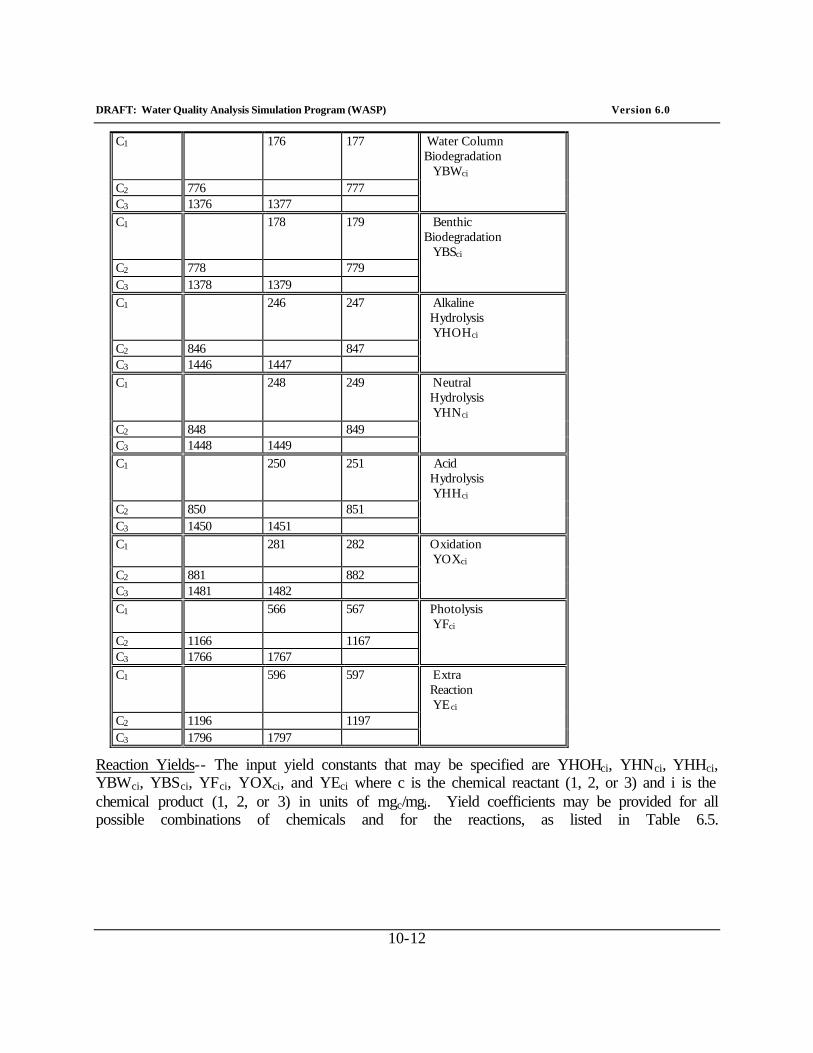
DRAFT: Water Quality Analysis Simulation Program (WASP) Version 6.0
10-12
C1 176 177 Water Column Biodegradation YBWci
C2 776 777 C3 1376 1377 C1 178 179 Benthic
Biodegradation YBSci
C2 778 779 C3 1378 1379 C1 246 247 Alkaline
Hydrolysis YHOHci
C2 846 847 C3 1446 1447 C1 248 249 Neutral
Hydrolysis YHNci
C2 848 849 C3 1448 1449 C1 250 251 Acid
Hydrolysis YHHci
C2 850 851 C3 1450 1451 C1 281 282 Oxidation
YOXci C2 881 882 C3 1481 1482 C1 566 567 Photolysis
YFci C2 1166 1167 C3 1766 1767 C1 596 597 Extra
Reaction YEci
C2 1196 1197 C3 1796 1797
Reaction Yields-- The input yield constants that may be specified are YHOHci, YHNci, YHHci, YBWci, YBSci, YFci, YOXci, and YEci where c is the chemical reactant (1, 2, or 3) and i is the chemical product (1, 2, or 3) in units of mgc/mgi. Yield coefficients may be provided for all possible combinations of chemicals and for the reactions, as listed in Table 6.5.
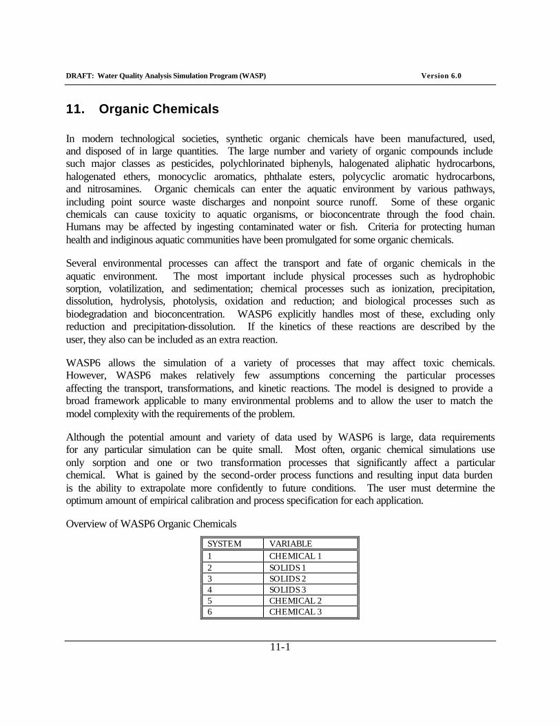
DRAFT: Water Quality Analysis Simulation Program (WASP) Version 6.0
11-1
11. Organic Chemicals
In modern technological societies, synthetic organic chemicals have been manufactured, used, and disposed of in large quantities. The large number and variety of organic compounds include such major classes as pesticides, polychlorinated biphenyls, halogenated aliphatic hydrocarbons, halogenated ethers, monocyclic aromatics, phthalate esters, polycyclic aromatic hydrocarbons, and nitrosamines. Organic chemicals can enter the aquatic environment by various pathways, including point source waste discharges and nonpoint source runoff. Some of these organic chemicals can cause toxicity to aquatic organisms, or bioconcentrate through the food chain. Humans may be affected by ingesting contaminated water or fish. Criteria for protecting human health and indiginous aquatic communities have been promulgated for some organic chemicals.
Several environmental processes can affect the transport and fate of organic chemicals in the aquatic environment. The most important include physical processes such as hydrophobic sorption, volatilization, and sedimentation; chemical processes such as ionization, precipitation, dissolution, hydrolysis, photolysis, oxidation and reduction; and biological processes such as biodegradation and bioconcentration. WASP6 explicitly handles most of these, excluding only reduction and precipitation-dissolution. If the kinetics of these reactions are described by the user, they also can be included as an extra reaction.
WASP6 allows the simulation of a variety of processes that may affect toxic chemicals. However, WASP6 makes relatively few assumptions concerning the particular processes affecting the transport, transformations, and kinetic reactions. The model is designed to provide a broad framework applicable to many environmental problems and to allow the user to match the model complexity with the requirements of the problem.
Although the potential amount and variety of data used by WASP6 is large, data requirements for any particular simulation can be quite small. Most often, organic chemical simulations use only sorption and one or two transformation processes that significantly affect a particular chemical. What is gained by the second-order process functions and resulting input data burden is the ability to extrapolate more confidently to future conditions. The user must determine the optimum amount of empirical calibration and process specification for each application.
Overview of WASP6 Organic Chemicals
SYSTEM VARIABLE 1 CHEMICAL 1 2 SOLIDS 1 3 SOLIDS 2 4 SOLIDS 3 5 CHEMICAL 2 6 CHEMICAL 3
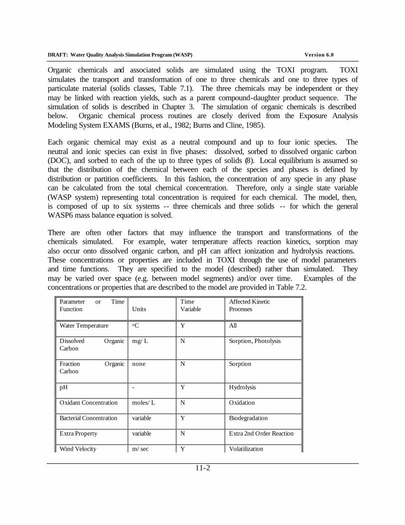
DRAFT: Water Quality Analysis Simulation Program (WASP) Version 6.0
11-2
Organic chemicals and associated solids are simulated using the TOXI program. TOXI simulates the transport and transformation of one to three chemicals and one to three types of particulate material (solids classes, Table 7.1). The three chemicals may be independent or they may be linked with reaction yields, such as a parent compound-daughter product sequence. The simulation of solids is described in Chapter 3. The simulation of organic chemicals is described below. Organic chemical process routines are closely derived from the Exposure Analysis Modeling System EXAMS (Burns, et al., 1982; Burns and Cline, 1985).
Each organic chemical may exist as a neutral compound and up to four ionic species. The neutral and ionic species can exist in five phases: dissolved, sorbed to dissolved organic carbon (DOC), and sorbed to each of the up to three types of solids (8). Local equilibrium is assumed so that the distribution of the chemical between each of the species and phases is defined by distribution or partition coefficients. In this fashion, the concentration of any specie in any phase can be calculated from the total chemical concentration. Therefore, only a single state variable (WASP system) representing total concentration is required for each chemical. The model, then, is composed of up to six systems -- three chemicals and three solids -- for which the general WASP6 mass balance equation is solved.
There are often other factors that may influence the transport and transformations of the chemicals simulated. For example, water temperature affects reaction kinetics, sorption may also occur onto dissolved organic carbon, and pH can affect ionization and hydrolysis reactions. These concentrations or properties are included in TOXI through the use of model parameters and time functions. They are specified to the model (described) rather than simulated. They may be varied over space (e.g. between model segments) and/or over time. Examples of the concentrations or properties that are described to the model are provided in Table 7.2.
Parameter or Time Function
Units
Time Variable
Affected Kinetic Processes
Water Temperature
oC
Y
All
Dissolved Organic Carbon
mg/L
N
Sorption, Photolysis
Fraction Organic Carbon
none
N
Sorption
pH
-
Y
Hydrolysis
Oxidant Concentration
moles/L
N
Oxidation
Bacterial Concentration
variable
Y
Biodegradation
Extra Property
variable
N
Extra 2nd Order Reaction
Wind Velocity m/sec Y Volatilization
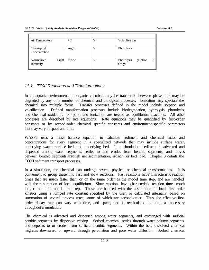
DRAFT: Water Quality Analysis Simulation Program (WASP) Version 6.0
11-3
Air Temperature
oC
Y
Volatilization
Chlorophyll a Concentration
mg/L
Y
Photolysis
Normalized Light Intensity
None
Y
Photolysis (Option 2 Only)
11.1. TOXI Reactions and Transformations
In an aquatic environment, an organic chemical may be transferred between phases and may be degraded by any of a number of chemical and biological processes. Ionization may speciate the chemical into multiple forms. Transfer processes defined in the model include sorption and volatilization. Defined transformation processes include biodegradation, hydrolysis, photolysis, and chemical oxidation. Sorption and ionization are treated as equilibrium reactions. All other processes are described by rate equations. Rate equations may be quantified by first-order constants or by second-order chemical specific constants and environment-specific parameters that may vary in space and time.
WASP6 uses a mass balance equation to calculate sediment and chemical mass and concentrations for every segment in a specialized network that may include surface water, underlying water, surface bed, and underlying bed. In a simulation, sediment is advected and dispersed among water segments, settles to and erodes from benthic segments, and moves between benthic segments through net sedimentation, erosion, or bed load. Chapter 3 details the TOXI sediment transport processes.
In a simulation, the chemical can undergo several physical or chemical transformations. It is convenient to group these into fast and slow reactions. Fast reactions have characteristic reaction times that are much faster than, or on the same order as the model time step, and are handled with the assumption of local equilibrium. Slow reactions have characteristic reaction times much longer than the model time step. These are handled with the assumption of local first order kinetics using a lumped rate constant specified by the user, or calculated internally, based on summation of several process rates, some of which are second-order. Thus, the effective first order decay rate can vary with time, and space, and is recalculated as often as necessary throughout a simulation.
The chemical is advected and dispersed among water segments, and exchanged with surficial benthic segments by dispersive mixing. Sorbed chemical settles through water column segments and deposits to or erodes from surficial benthic segments. Within the bed, dissolved chemical migrates downward or upward through percolation and pore water diffusion. Sorbed chemical
DRAFT: Water Quality Analysis Simulation Program (WASP) Version 6.0
11-4
migrates downward or upward through net sedimentation or erosion. Both rate constants and equilibrium coefficients must be estimated in most toxic chemical studies. Although these can be calculated internally from chemical properties and local environmental characteristics, site-specific calibration or testing is desirable.
Some limitations should be kept in mind when applying TOXI. First, chemical concentrations should be near trace levels, i.e., below half the solubility or 10-5 molar. At higher concentrations, the assumptions of linear partitioning and transformation begin to break down. Chemical density may become important, particularly near the source, such as in a spill. Large concentrations can affect key environmental characteristics, such as pH or bacterial populations, thus altering transformation rates. TOXI does not include such feedback phenomena.
11.2. Model Implementation
To simulate organic chemicals with WASP6, use the preprocessor or text editor to create a TOXI input file. The model input dataset and the input parameters will be similar to those for the conservative tracer model as described in Chapter 2. To those basic parameters, the user will add benthic segments, solids transport rates, and transformation parameters. During the simulation, solids and organic chemicals will be transported both by the water column advection and dispersion rates and by these solids transport rates.
In WASP6, solids transport rates in the water column and the bed are input via up to three solids transport fields, as described in Chapter 3. The transport of the particulate fraction of organic chemicals follows the solids flows. The user must specify the dissolved fraction (i.e. 0.0) and the solids transport field for each simulated solid under initial conditions. To simulate total solids, solids 1 must be used.
11.2.1. Model Input Parameters
Input parameters are prepared for WASP6 in four major sections of the preprocessor -- environment, transport, boundaries, and transformation. The organic chemical input parameters comprising the first three sections are identical to those in the simple toxicant model. The user is referred to Section 6.2 for a summary of these input parameters. This section, and the rest of this chapter, describes the organic chemical reaction parameters.
11.2.2. Transformation Parameters
This group of parameters includes spatially variable parameters, constants, and kinetic time functions for the water quality constituents being simulated. The organic chemical reactions and model input parameters are described in individual sections below. Because water temperature can affect every chemical reaction, it is described here.
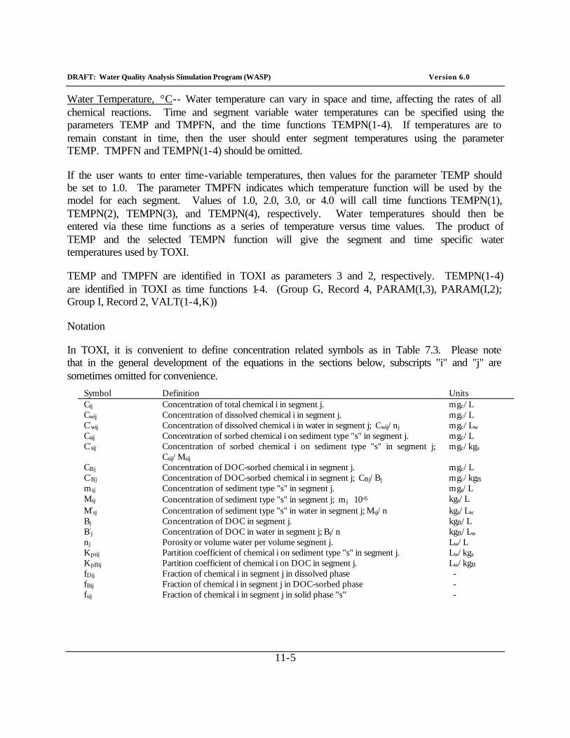
DRAFT: Water Quality Analysis Simulation Program (WASP) Version 6.0
11-5
Water Temperature, °C-- Water temperature can vary in space and time, affecting the rates of all chemical reactions. Time and segment variable water temperatures can be specified using the parameters TEMP and TMPFN, and the time functions TEMPN(1-4). If temperatures are to remain constant in time, then the user should enter segment temperatures using the parameter TEMP. TMPFN and TEMPN(1-4) should be omitted.
If the user wants to enter time-variable temperatures, then values for the parameter TEMP should be set to 1.0. The parameter TMPFN indicates which temperature function will be used by the model for each segment. Values of 1.0, 2.0, 3.0, or 4.0 will call time functions TEMPN(1), TEMPN(2), TEMPN(3), and TEMPN(4), respectively. Water temperatures should then be entered via these time functions as a series of temperature versus time values. The product of TEMP and the selected TEMPN function will give the segment and time specific water temperatures used by TOXI.
TEMP and TMPFN are identified in TOXI as parameters 3 and 2, respectively. TEMPN(1-4) are identified in TOXI as time functions 1-4. (Group G, Record 4, PARAM(I,3), PARAM(I,2); Group I, Record 2, VALT(1-4,K))
Notation
In TOXI, it is convenient to define concentration related symbols as in Table 7.3. Please note that in the general development of the equations in the sections below, subscripts "i" and "j" are sometimes omitted for convenience.
Symbol Definition Units Cij Concentration of total chemical i in segment j. mgc/L Cwij Concentration of dissolved chemical i in segment j. mgc/L C'wij Concentration of dissolved chemical i in water in segment j; Cwij/nj mgc/Lw Csij Concentration of sorbed chemical i on sediment type "s" in segment j. mgc/L C'sij Concentration of sorbed chemical i on sediment type "s" in segment j;
Csij/Msij mgc/kgs
CBj Concentration of DOC-sorbed chemical i in segment j. mgc/L C'Bj Concentration of DOC-sorbed chemical i in segment j; CBj/Bj mgc/kgB msj Concentration of sediment type "s" in segment j. mgs/L Msj Concentration of sediment type "s" in segment j; m j ⋅ 10-6 kgs/L M'sj Concentration of sediment type "s" in water in segment j; Msj/n kgs/Lw Bj Concentration of DOC in segment j. kgB/L B'j Concentration of DOC in water in segment j; Bj/n kgB/Lw nj Porosity or volume water per volume segment j. Lw/L Kpsij Partition coefficient of chemical i on sediment type "s" in segment j. Lw/kgs KpBij Partition coefficient of chemical i on DOC in segment j. Lw/kgB fDij Fraction of chemical i in segment j in dissolved phase - fBij Fraction of chemical i in segment j in DOC-sorbed phase - fsij Fraction of chemical i in segment j in solid phase "s" -
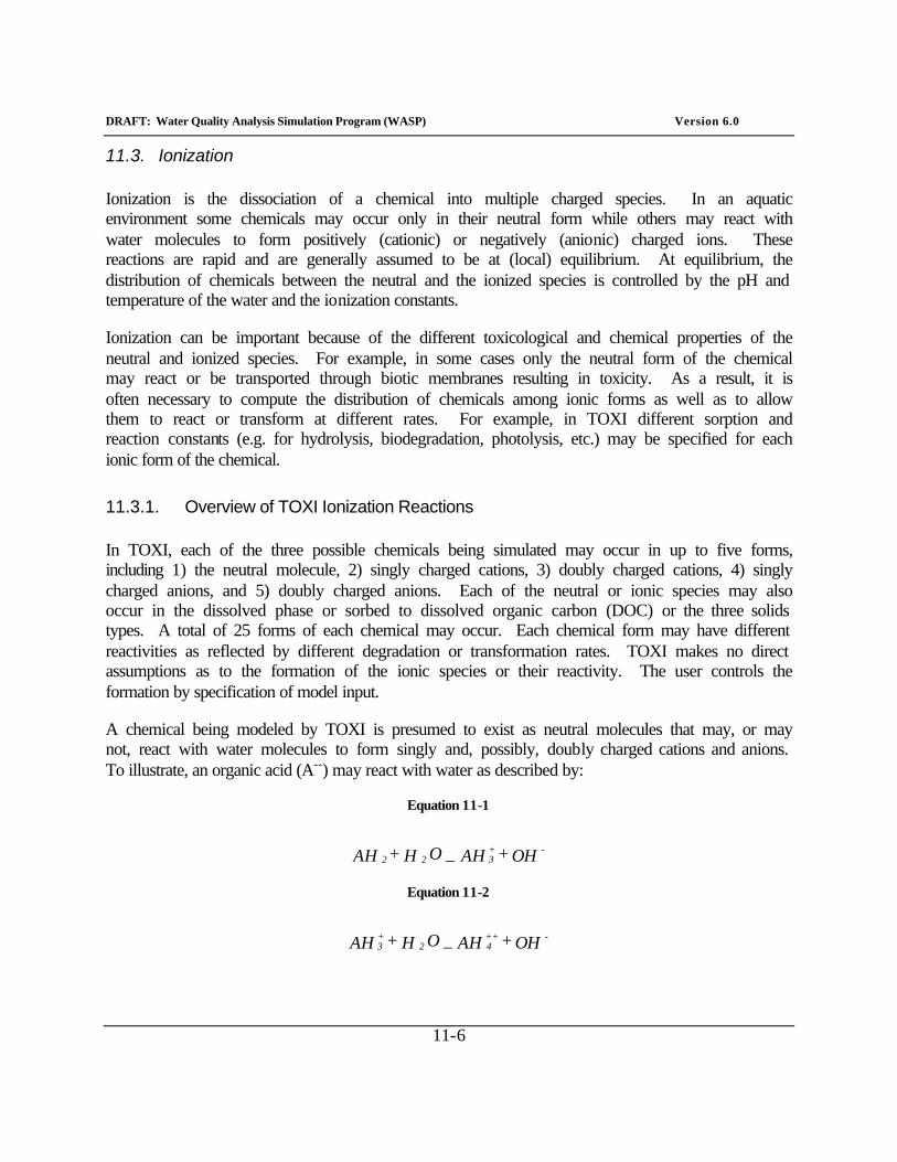
DRAFT: Water Quality Analysis Simulation Program (WASP) Version 6.0
11-6
11.3. Ionization
Ionization is the dissociation of a chemical into multiple charged species. In an aquatic environment some chemicals may occur only in their neutral form while others may react with water molecules to form positively (cationic) or negatively (anionic) charged ions. These reactions are rapid and are generally assumed to be at (local) equilibrium. At equilibrium, the distribution of chemicals between the neutral and the ionized species is controlled by the pH and temperature of the water and the ionization constants.
Ionization can be important because of the different toxicological and chemical properties of the neutral and ionized species. For example, in some cases only the neutral form of the chemical may react or be transported through biotic membranes resulting in toxicity. As a result, it is often necessary to compute the distribution of chemicals among ionic forms as well as to allow them to react or transform at different rates. For example, in TOXI different sorption and reaction constants (e.g. for hydrolysis, biodegradation, photolysis, etc.) may be specified for each ionic form of the chemical.
11.3.1. Overview of TOXI Ionization Reactions
In TOXI, each of the three possible chemicals being simulated may occur in up to five forms, including 1) the neutral molecule, 2) singly charged cations, 3) doubly charged cations, 4) singly charged anions, and 5) doubly charged anions. Each of the neutral or ionic species may also occur in the dissolved phase or sorbed to dissolved organic carbon (DOC) or the three solids types. A total of 25 forms of each chemical may occur. Each chemical form may have different reactivities as reflected by different degradation or transformation rates. TOXI makes no direct assumptions as to the formation of the ionic species or their reactivity. The user controls the formation by specification of model input.
A chemical being modeled by TOXI is presumed to exist as neutral molecules that may, or may not, react with water molecules to form singly and, possibly, doubly charged cations and anions. To illustrate, an organic acid (A--) may react with water as described by:
Equation 11-1
OH + AH OH + AH - + 3 2 2 _
Equation 11-2
OH + AH OH + AH - ++ 4 2
+ 3 _
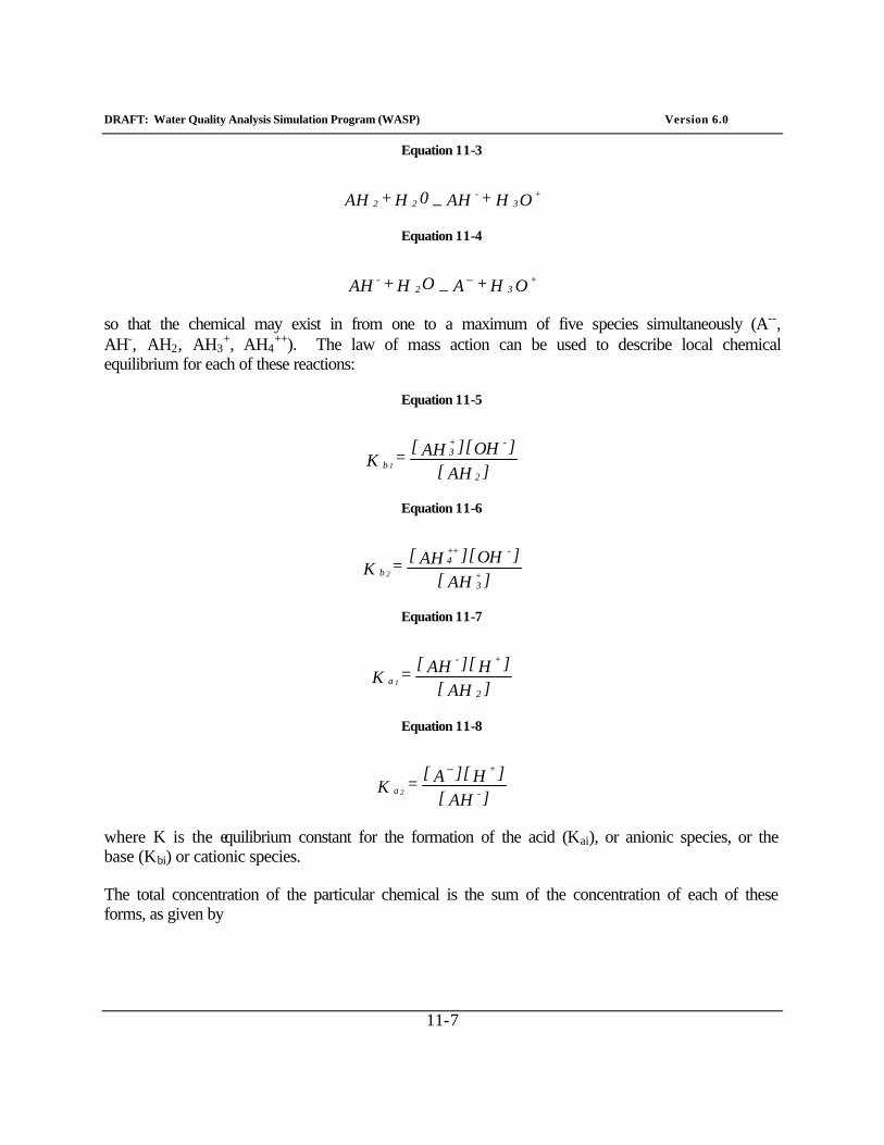
DRAFT: Water Quality Analysis Simulation Program (WASP) Version 6.0
11-7
Equation 11-3
OH + AH 0H + AH + 3
- 2 2 _
Equation 11-4
OH + A OH + AH + 3
-- 2
- _
so that the chemical may exist in from one to a maximum of five species simultaneously (A--, AH-, AH2, AH3
+, AH4++). The law of mass action can be used to describe local chemical
equilibrium for each of these reactions:
Equation 11-5
]AH[]OH][AH[
= K2
- + 3
b 1
Equation 11-6
]AH[]OH][AH[
= K + 3
- ++ 4
b 2
Equation 11-7
]AH[]H][AH[
= K2
+ -
a 1
Equation 11-8
]AH[]H][A[
= K -
+ --
a 2
where K is the equilibrium constant for the formation of the acid (Kai), or anionic species, or the base (Kbi) or cationic species.
The total concentration of the particular chemical is the sum of the concentration of each of these forms, as given by
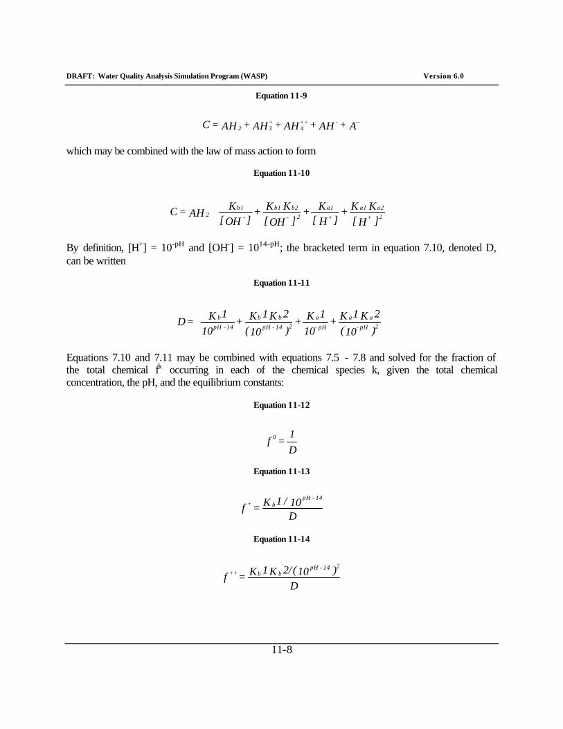
DRAFT: Water Quality Analysis Simulation Program (WASP) Version 6.0
11-8
Equation 11-9
A + AH + AH + AH + AH = C ---++4
+32
which may be combined with the law of mass action to form
Equation 11-10
]H[K K +
]H[K +
]OH[K K +
]OH[K AH = C 2+
a2a1
+
a12-
b2b1
-
b12
By definition, [H+] = 10-pH and [OH-] = 1014-pH; the bracketed term in equation 7.10, denoted D, can be written
Equation 11-11
)10(
2K 1K + 10
1K + )10(
2K 1K + 10
1K = D 2pH-
aa
pH-
a214 - pH
bb
14 - pH
b
Equations 7.10 and 7.11 may be combined with equations 7.5 - 7.8 and solved for the fraction of the total chemical fk occurring in each of the chemical species k, given the total chemical concentration, the pH, and the equilibrium constants:
Equation 11-12
D1
= f 0
Equation 11-13
D10 / 1K = f
14 - pHb+
Equation 11-14
D)10(2/K 1K = f
214 - pHbb++
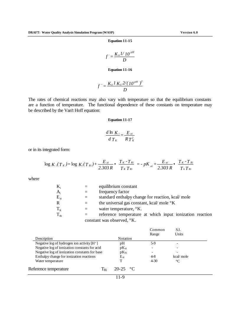
DRAFT: Water Quality Analysis Simulation Program (WASP) Version 6.0
11-9
Equation 11-15
D101/K = f
-pHa-
Equation 11-16
D)10(2/K 1K = f
2-pHaa--
The rates of chemical reactions may also vary with temperature so that the equilibrium constants are a function of temperature. The functional dependence of these constants on temperature may be described by the Van't Hoff equation:
Equation 11-17
T RE =
T dK d
2K
ai
K
i ln
or in its integrated form:
•
•T TT - T
R 2.303E + pK - =
T TT - T
R 2.303E + )T(K = )T(K
Rik
RiKai ai
RiK
RiKai RiiKi loglog
where
Ki = equilibrium constant Ai = frequency factor Eai = standard enthalpy change for reaction, kcal/mole R = the universal gas constant, kcal/mole °K TK = water temperature, °K. TRi = reference temperature at which input ionization reaction
constant was observed, °K.
Common Range
S.I. Units
Description Notation Negative log of hydrogen ion activity [H+] pH 5-9 - Negative log of ionization constants for acid pKai - - Negative log of ionization constants for base pKbi - - Enthalpy change for ionization reactions Eai 4-8 kcal/mole Water temperature T 4-30 °C
Reference temperature TRi 20-25 °C
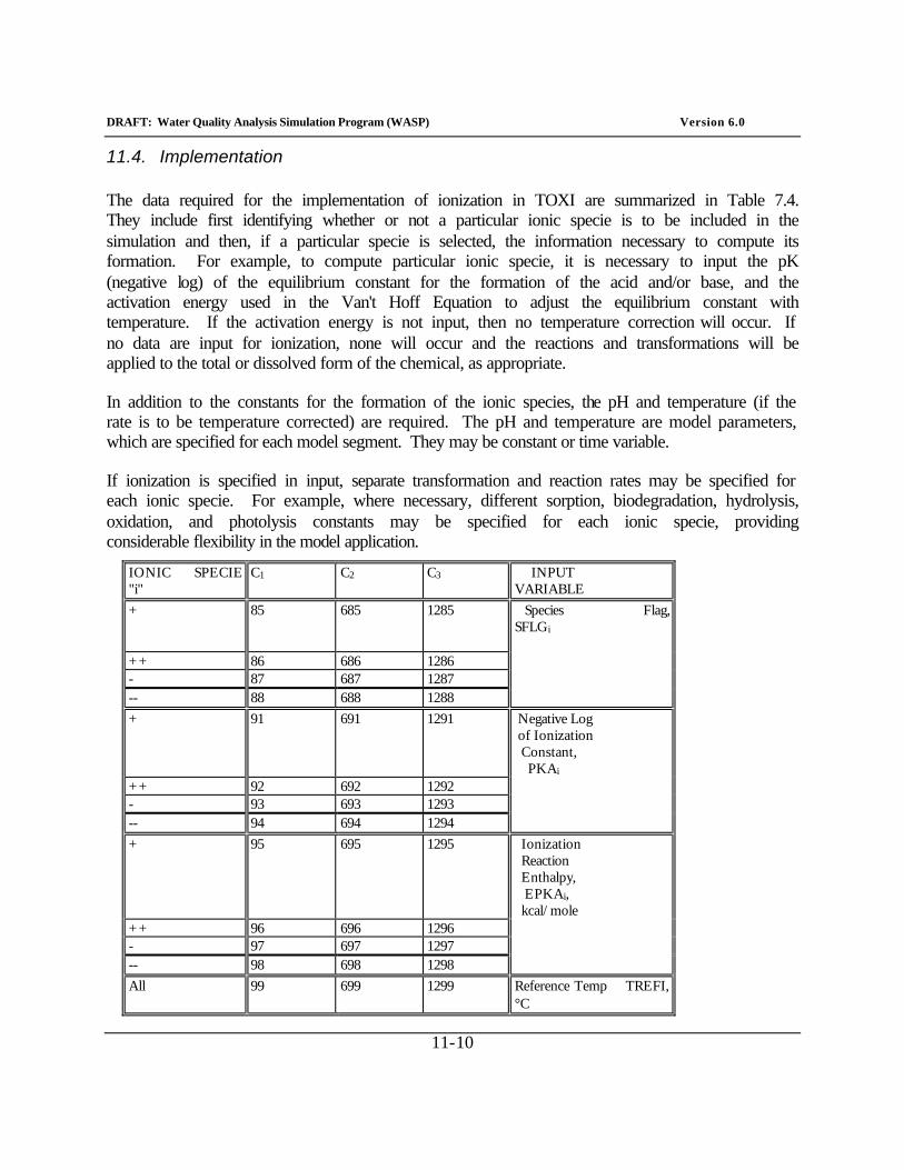
DRAFT: Water Quality Analysis Simulation Program (WASP) Version 6.0
11-10
11.4. Implementation
The data required for the implementation of ionization in TOXI are summarized in Table 7.4. They include first identifying whether or not a particular ionic specie is to be included in the simulation and then, if a particular specie is selected, the information necessary to compute its formation. For example, to compute particular ionic specie, it is necessary to input the pK (negative log) of the equilibrium constant for the formation of the acid and/or base, and the activation energy used in the Van't Hoff Equation to adjust the equilibrium constant with temperature. If the activation energy is not input, then no temperature correction will occur. If no data are input for ionization, none will occur and the reactions and transformations will be applied to the total or dissolved form of the chemical, as appropriate.
In addition to the constants for the formation of the ionic species, the pH and temperature (if the rate is to be temperature corrected) are required. The pH and temperature are model parameters, which are specified for each model segment. They may be constant or time variable.
If ionization is specified in input, separate transformation and reaction rates may be specified for each ionic specie. For example, where necessary, different sorption, biodegradation, hydrolysis, oxidation, and photolysis constants may be specified for each ionic specie, providing considerable flexibility in the model application.
IONIC SPECIE "i"
C1 C2 C3 INPUT VARIABLE
+ 85 685 1285 Species Flag, SFLGi
++ 86 686 1286 - 87 687 1287 -- 88 688 1288
+ 91 691 1291 Negative Log of Ionization Constant, PKAi
++ 92 692 1292 - 93 693 1293 -- 94 694 1294
+ 95 695 1295 Ionization Reaction Enthalpy, EPKAi, kcal/mole
++ 96 696 1296 - 97 697 1297 -- 98 698 1298
All 99 699 1299 Reference Temp TREFI, °C
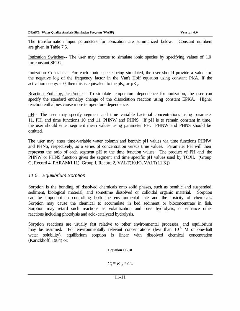
DRAFT: Water Quality Analysis Simulation Program (WASP) Version 6.0
11-11
The transformation input parameters for ionization are summarized below. Constant numbers are given in Table 7.5.
Ionization Switches-- The user may choose to simulate ionic species by specifying values of 1.0 for constant SFLG.
Ionization Constants-- For each ionic specie being simulated, the user should provide a value for the negative log of the frequency factor in the Van't Hoff equation using constant PKA. If the activation energy is 0, then this is equivalent to the pKa or pKb.
Reaction Enthalpy, kcal/mole-- To simulate temperature dependence for ionization, the user can specify the standard enthalpy change of the dissociation reaction using constant EPKA. Higher reaction enthalpies cause more temperature dependence.
pH-- The user may specify segment and time variable bacterial concentrations using parameter 11, PH, and time functions 10 and 11, PHNW and PHNS. If pH is to remain constant in time, the user should enter segment mean values using parameter PH. PHNW and PHNS should be omitted.
The user may enter time-variable water column and benthic pH values via time functions PHNW and PHNS, respectively, as a series of concentration versus time values. Parameter PH will then represent the ratio of each segment pH to the time function values. The product of PH and the PHNW or PHNS function gives the segment and time specific pH values used by TOXI. (Group G, Record 4, PARAM(I,11); Group I, Record 2, VALT(10,K), VALT(11,K))
11.5. Equilibrium Sorption
Sorption is the bonding of dissolved chemicals onto solid phases, such as benthic and suspended sediment, biological material, and sometime dissolved or colloidal organic material. Sorption can be important in controlling both the environmental fate and the toxicity of chemicals. Sorption may cause the chemical to accumulate in bed sediment or bioconcentrate in fish. Sorption may retard such reactions as volatilization and base hydrolysis, or enhance other reactions including photolysis and acid-catalyzed hydrolysis.
Sorption reactions are usually fast relative to other environmental processes, and equilibrium may be assumed. For environmentally relevant concentrations (less than 10-5 M or one-half water solubility), equilibrium sorption is linear with dissolved chemical concentration (Karickhoff, 1984) or:
Equation 11-18
C K = C ,wps
,s •
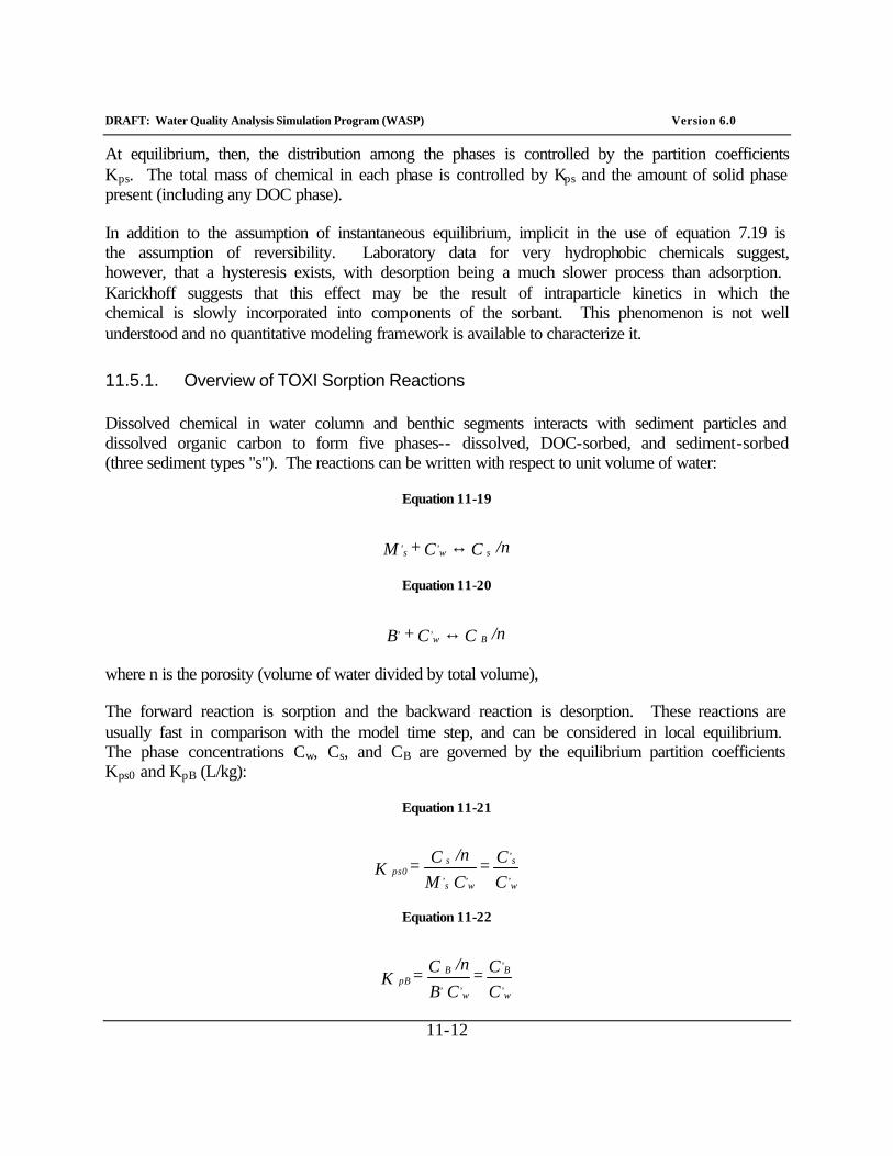
DRAFT: Water Quality Analysis Simulation Program (WASP) Version 6.0
11-12
At equilibrium, then, the distribution among the phases is controlled by the partition coefficients Kps. The total mass of chemical in each phase is controlled by Kps and the amount of solid phase present (including any DOC phase).
In addition to the assumption of instantaneous equilibrium, implicit in the use of equation 7.19 is the assumption of reversibility. Laboratory data for very hydrophobic chemicals suggest, however, that a hysteresis exists, with desorption being a much slower process than adsorption. Karickhoff suggests that this effect may be the result of intraparticle kinetics in which the chemical is slowly incorporated into components of the sorbant. This phenomenon is not well understood and no quantitative modeling framework is available to characterize it.
11.5.1. Overview of TOXI Sorption Reactions
Dissolved chemical in water column and benthic segments interacts with sediment particles and dissolved organic carbon to form five phases-- dissolved, DOC-sorbed, and sediment-sorbed (three sediment types "s"). The reactions can be written with respect to unit volume of water:
Equation 11-19
/n C C + M s, w
, s ↔
Equation 11-20
/n C C + B B , w
, ↔
where n is the porosity (volume of water divided by total volume),
The forward reaction is sorption and the backward reaction is desorption. These reactions are usually fast in comparison with the model time step, and can be considered in local equilibrium. The phase concentrations Cw, Cs, and CB are governed by the equilibrium partition coefficients Kps0 and KpB (L/kg):
Equation 11-21
CC =
C M
/n C = K , w
, s
, w
, s
sps0
Equation 11-22
CC =
C B
/n C = K , w
,B
, w
,
B pB
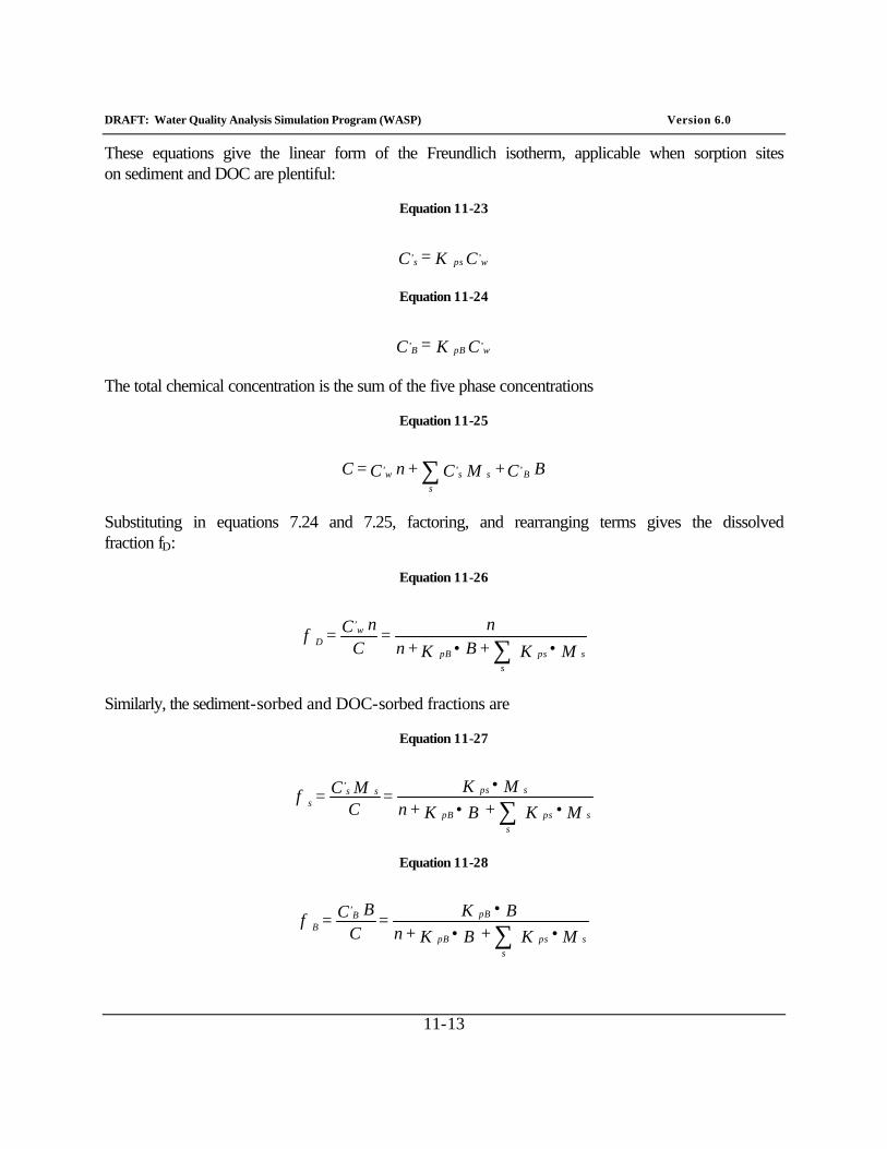
DRAFT: Water Quality Analysis Simulation Program (WASP) Version 6.0
11-13
These equations give the linear form of the Freundlich isotherm, applicable when sorption sites on sediment and DOC are plentiful:
Equation 11-23
C K = C , wps
, s
Equation 11-24
C K = C , wpB
,B
The total chemical concentration is the sum of the five phase concentrations
Equation 11-25
B C + M C + n C = C ,B s
, s
s
, w ∑
Substituting in equations 7.24 and 7.25, factoring, and rearranging terms gives the dissolved fraction fD:
Equation 11-26
M K + B K + nn
= C
n C = f sps
spB
, w
D •• ∑
Similarly, the sediment-sorbed and DOC-sorbed fractions are
Equation 11-27
M K + B K + nM K =
CM C = f
sps s
pB
sps s, s
s •••
∑
Equation 11-28
M K + B K + nB K =
CB C = f
sps s
pB
pB ,B
B •••
∑
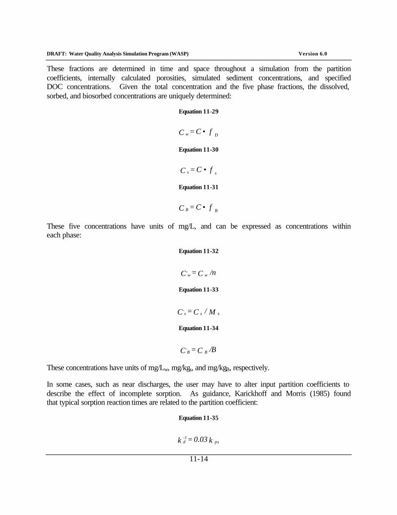
DRAFT: Water Quality Analysis Simulation Program (WASP) Version 6.0
11-14
These fractions are determined in time and space throughout a simulation from the partition coefficients, internally calculated porosities, simulated sediment concentrations, and specified DOC concentrations. Given the total concentration and the five phase fractions, the dissolved, sorbed, and biosorbed concentrations are uniquely determined:
Equation 11-29
f C = C D w •
Equation 11-30
f C = C s s •
Equation 11-31
f C = C B B •
These five concentrations have units of mg/L, and can be expressed as concentrations within each phase:
Equation 11-32
/n C = C w, w
Equation 11-33
M/ C = C s s, s
Equation 11-34
/B C = C B ,B
These concentrations have units of mg/Lw, mg/kgs, and mg/kgB, respectively.
In some cases, such as near discharges, the user may have to alter input partition coefficients to describe the effect of incomplete sorption. As guidance, Karickhoff and Morris (1985) found that typical sorption reaction times are related to the partition coefficient:
Equation 11-35
k 0.03 = k ps 1-
d
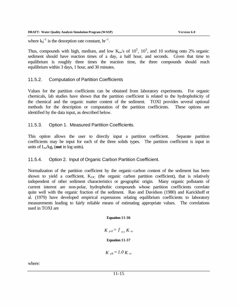
DRAFT: Water Quality Analysis Simulation Program (WASP) Version 6.0
11-15
where kd-1 is the desorption rate constant, hr-1.
Thus, compounds with high, medium, and low Kow's of 105, 103, and 10 sorbing onto 2% organic sediment should have reaction times of a day, a half hour, and seconds. Given that time to equilibrium is roughly three times the reaction time, the three compounds should reach equilibrium within 3 days, 1 hour, and 30 minutes.
11.5.2. Computation of Partition Coefficients
Values for the partition coefficients can be obtained from laboratory experiments. For organic chemicals, lab studies have shown that the partition coefficient is related to the hydrophobicity of the chemical and the organic matter content of the sediment. TOXI provides several optional methods for the description or computation of the partition coefficients. These options are identified by the data input, as described below.
11.5.3. Option 1. Measured Partition Coefficients.
This option allows the user to directly input a partition coefficient. Separate partition coefficients may be input for each of the three solids types. The partition coefficient is input in units of Lw/kgs (not in log units).
11.5.4. Option 2. Input of Organic Carbon Partition Coefficient.
Normalization of the partition coefficient by the organic-carbon content of the sediment has been shown to yield a coefficient, KOC (the organic carbon partition coefficient), that is relatively independent of other sediment characteristics or geographic origin. Many organic pollutants of current interest are non-polar, hydrophobic compounds whose partition coefficients correlate quite well with the organic fraction of the sediment. Rao and Davidson (1980) and Karickhoff et al. (1979) have developed empirical expressions relating equilibrium coefficients to laboratory measurements leading to fairly reliable means of estimating appropriate values. The correlations used in TOXI are
Equation 11-36
K f = K oc ocs ps0
Equation 11-37
K 1.0 = K oc pB
where:
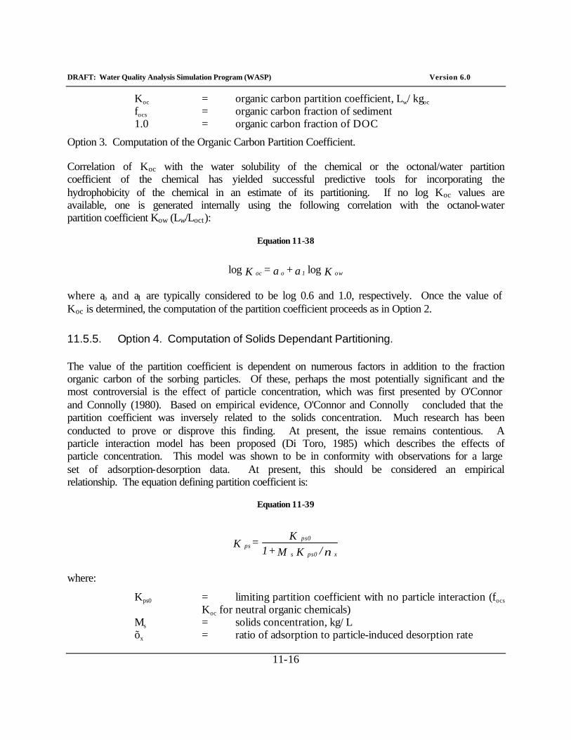
DRAFT: Water Quality Analysis Simulation Program (WASP) Version 6.0
11-16
Koc = organic carbon partition coefficient, Lw/kgoc focs = organic carbon fraction of sediment 1.0 = organic carbon fraction of DOC
Option 3. Computation of the Organic Carbon Partition Coefficient.
Correlation of Koc with the water solubility of the chemical or the octonal/water partition coefficient of the chemical has yielded successful predictive tools for incorporating the hydrophobicity of the chemical in an estimate of its partitioning. If no log Koc values are available, one is generated internally using the following correlation with the octanol-water partition coefficient Kow (Lw/Loct):
Equation 11-38
K a + a = K ow 1 o oc loglog
where ao and a1 are typically considered to be log 0.6 and 1.0, respectively. Once the value of Koc is determined, the computation of the partition coefficient proceeds as in Option 2.
11.5.5. Option 4. Computation of Solids Dependant Partitioning.
The value of the partition coefficient is dependent on numerous factors in addition to the fraction organic carbon of the sorbing particles. Of these, perhaps the most potentially significant and the most controversial is the effect of particle concentration, which was first presented by O'Connor and Connolly (1980). Based on empirical evidence, O'Connor and Connolly concluded that the partition coefficient was inversely related to the solids concentration. Much research has been conducted to prove or disprove this finding. At present, the issue remains contentious. A particle interaction model has been proposed (Di Toro, 1985) which describes the effects of particle concentration. This model was shown to be in conformity with observations for a large set of adsorption-desorption data. At present, this should be considered an empirical relationship. The equation defining partition coefficient is:
Equation 11-39
ν x ps0 s
ps0 ps / K M + 1
K = K
where:
Kps0 = limiting partition coefficient with no particle interaction (focs Koc for neutral organic chemicals)
Ms = solids concentration, kg/L õx = ratio of adsorption to particle-induced desorption rate
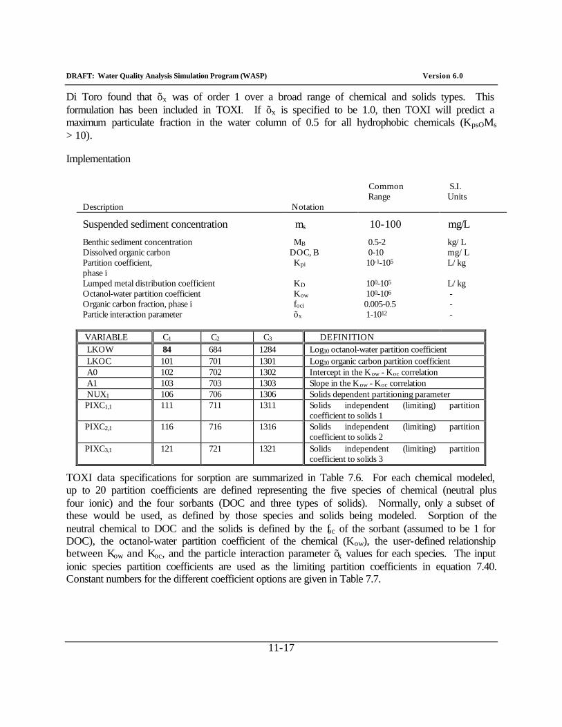
DRAFT: Water Quality Analysis Simulation Program (WASP) Version 6.0
11-17
Di Toro found that õx was of order 1 over a broad range of chemical and solids types. This formulation has been included in TOXI. If õx is specified to be 1.0, then TOXI will predict a maximum particulate fraction in the water column of 0.5 for all hydrophobic chemicals (KpsOMs > 10).
Implementation
Common Range
S.I. Units
Description Notation
Suspended sediment concentration ms 10-100 mg/L
Benthic sediment concentration MB 0.5-2 kg/L Dissolved organic carbon DOC, B 0-10 mg/L Partition coefficient, phase i
Kpi 10-1-105 L/kg
Lumped metal distribution coefficient KD 100-105 L/kg Octanol-water partition coefficient Kow 100-106 - Organic carbon fraction, phase i foci 0.005-0.5 - Particle interaction parameter õx 1-1012 - VARIABLE C1 C2 C3 DEFINITION LKOW 84 684 1284 Log10 octanol-water partition coefficient LKOC 101 701 1301 Log10 organic carbon partition coefficient A0 102 702 1302 Intercept in the Kow - Koc correlation A1 103 703 1303 Slope in the Kow - Koc correlation NUX1 106 706 1306 Solids dependent partitioning parameter PIXC1,1 111 711 1311 Solids independent (limiting) partition
coefficient to solids 1 PIXC2,1 116 716 1316 Solids independent (limiting) partition
coefficient to solids 2 PIXC3,1 121 721 1321 Solids independent (limiting) partition
coefficient to solids 3
TOXI data specifications for sorption are summarized in Table 7.6. For each chemical modeled, up to 20 partition coefficients are defined representing the five species of chemical (neutral plus four ionic) and the four sorbants (DOC and three types of solids). Normally, only a subset of these would be used, as defined by those species and solids being modeled. Sorption of the neutral chemical to DOC and the solids is defined by the foc of the sorbant (assumed to be 1 for DOC), the octanol-water partition coefficient of the chemical (Kow), the user-defined relationship between Kow and Koc, and the particle interaction parameter õx values for each species. The input ionic species partition coefficients are used as the limiting partition coefficients in equation 7.40. Constant numbers for the different coefficient options are given in Table 7.7.
DRAFT: Water Quality Analysis Simulation Program (WASP) Version 6.0
11-18
11.5.6. Option 1: Measured Partition Coefficients.
For each chemical simulated, separate partition coefficients may be entered for sorption of the neutral molecule and up to 4 ionic species onto each of the three possible solids types and DOC. The partition coefficient is input in units of Lw/kgs (not in log units). If a partition coefficient is specified it will be used regardless. The user is referred to Chapter 6 for details on directly specifying partition coefficients.
Solids Partition Coefficient, L/kg-- The user may directly specify partition coefficients to solids using constant PIXC. Constant numbers for sorption of the neutral molecule are given in Table 7.7.
DOC Partition Coefficient-- The user may specify partition coefficients for sorption of ionic species to DOC using constant PIDOC.
11.5.7. Option 2: Input of Organic Carbon Partition Coefficient.
Under this option the user inputs the log (base 10) of the organic carbon partition coefficient (Koc). In addition, the user should also input the fraction organic carbon for each of the solids types simulated. The fraction organic carbon for dissolved organic carbon is assumed to be 1.0. The fraction organic carbon and dissolved organic carbon concentration are model parameters, which may be specified for each model segment. If a value for the partition coefficient (Kp, Option 1) is input, then Koc will not be used.
Organic Carbon Partition Coefficient, L/kg-- The user may specify the log10 of the organic carbon partition coefficient using constant LKOC. Constant numbers are given in Table 7.7.
Fraction Organic Carbon-- The user should specify the segment variable fraction organic carbon for each solids type simulated using parameters FOC(I,1), FOC(I,2), and FOC(I,3). Parameter numbers for solids 1, 2, and 3 are 7, 8, and 9, respectively.
Dissolved Organic Carbon, mg/L-- The user may specify segment variable dissolved organic carbon concentrations using parameter 6, DOC.
11.5.8. Option 3: Computation of the Organic Carbon Partition Coefficient.
Under this option, the user allows the model to compute the Koc from a specified octanol water partition coefficient (Kow). The model then computes the Koc using equation 7.39. This option will not be used if values for the log (Koc) are input.
Octanol-Water Partition Coefficient, Lw/Lo-- The user may specify the log10 of the octanol-water partition coefficient using constant LKOC. Constant numbers are given in Table 7.7.
DRAFT: Water Quality Analysis Simulation Program (WASP) Version 6.0
11-19
Correlation Coefficients-- The user should specify correlation coefficients relating Kow with Koc using constants A0 and A1. A0 and A1 are the intercept and the slope in the correlation described by equation 7.39. Default values are log 0.6 and 1.0, respectively. If these constants are not entered, then, the correlation becomes Koc = 0.6 Kow. Constant numbers are given in Table 7.7.
Fraction Organic Carbon-- The user should specify the segment variable fraction organic carbon for each solids type simulated using parameters FOC(I,1), FOC(I,2), and FOC(I,3). Parameter numbers for solids 1, 2, and 3 are 7, 8, and 9, respectively.
Dissolved Organic Carbon, mg/L-- The user may specify segment variable dissolved organic carbon concentrations using parameter 6, DOC.
11.5.9. Option 4: Solids Dependant Partitioning.
The user may include the effect of solids concentration on adsorption by using a value of õx of order 1 (see Di Toro, 1985 for more detail). If the user does not provide an input value for õx, the default value will eliminate any solids effect on the partition coefficient. Since collision induced desorption is only expected to occur in the water column, solids dependant partitioning is only computed for water column segments (where porosity is greater that 0.99). In addition to the partical interaction parameter, the user must provide for a partition coefficient following option 1, 2, or 3 described above.
Particle Interaction Parameter-- The user may implement solids dependent partitioning by specifying an appropriate value for constant NUX. A value of order 1 will cause the input partition coefficient to decrease with increasing suspended solids, following equation 7.40. Larger values of NUX will reduce the solids effect on partitioning. The default value of 1012 effectively eliminates this behavior. Constant numbers for the solids effect on the neutral molecule are given in Table 7.7.
11.6. Volatilization
Volatilization is the movement of chemical across the air-water interface as the dissolved neutral concentration attempts to equilibrate with the gas phase concentration. Equilibrium occurs when the partial pressure exerted by the chemical in solution equals the partial pressure of the chemical in the overlying atmosphere. The rate of exchange is proportional to the gradient between the dissolved concentration and the concentration in the overlying atmosphere and the conductivity across the interface of the two fluids. The conductivity is influenced by both chemical properties (molecular weight, Henry's Law constant) and environmental conditions at the air-water interface (turbulence-controlled by wind speed, current velocity, and water depth).
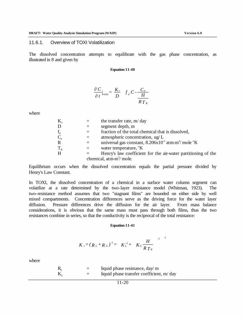
DRAFT: Water Quality Analysis Simulation Program (WASP) Version 6.0
11-20
11.6.1. Overview of TOXI Volatilization
The dissolved concentration attempts to equilibrate with the gas phase concentration, as illustrated in 8 and given by
Equation 11-40
∂∂
T RHC - C f
DK = |
t C
K
ad
vvolat
where
Kv = the transfer rate, m/day D = segment depth, m fd = fraction of the total chemical that is dissolved, Ca = atmospheric concentration, ug/L R = universal gas constant, 8.206x10⁻⁵ atm-m3/mole oK TK = water temperature, oK H = Henry's law coefficient for the air-water partitioning of the
chemical, atm-m3/mole.
Equilibrium occurs when the dissolved concentration equals the partial pressure divided by Henry's Law Constant.
In TOXI, the dissolved concentration of a chemical in a surface water column segment can volatilize at a rate determined by the two-layer resistance model (Whitman, 1923). The two-resistance method assumes that two "stagnant films" are bounded on either side by well mixed compartments. Concentration differences serve as the driving force for the water layer diffusion. Pressure differences drive the diffusion for the air layer. From mass balance considerations, it is obvious that the same mass must pass through both films, thus the two resistances combine in series, so that the conductivity is the reciprocal of the total resistance:
Equation 11-41
T RH
K + K = )R + R( = KK
G
1-
1- L
1-
G L 1-
v
where
RL = liquid phase resistance, day/m KL = liquid phase transfer coefficient, m/day
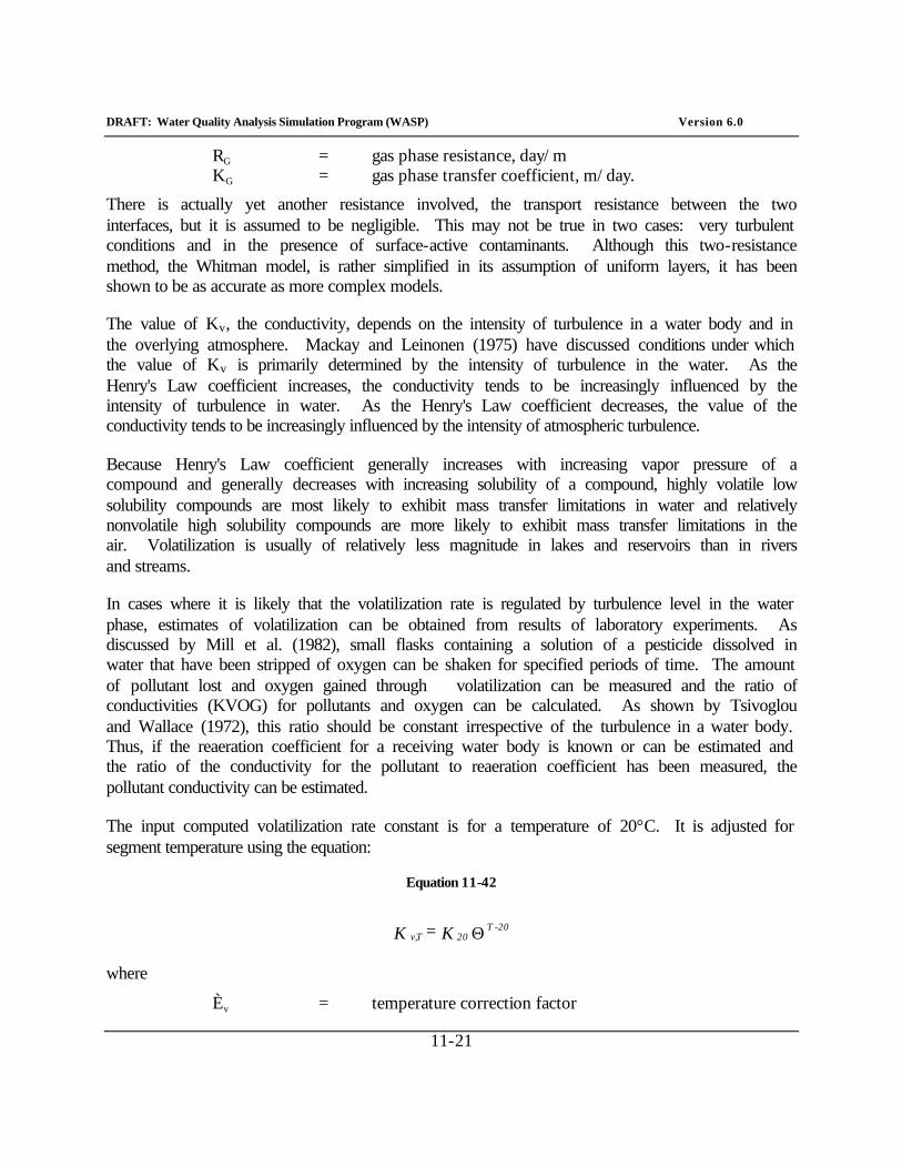
DRAFT: Water Quality Analysis Simulation Program (WASP) Version 6.0
11-21
RG = gas phase resistance, day/m KG = gas phase transfer coefficient, m/day.
There is actually yet another resistance involved, the transport resistance between the two interfaces, but it is assumed to be negligible. This may not be true in two cases: very turbulent conditions and in the presence of surface-active contaminants. Although this two-resistance method, the Whitman model, is rather simplified in its assumption of uniform layers, it has been shown to be as accurate as more complex models.
The value of Kv, the conductivity, depends on the intensity of turbulence in a water body and in the overlying atmosphere. Mackay and Leinonen (1975) have discussed conditions under which the value of Kv is primarily determined by the intensity of turbulence in the water. As the Henry's Law coefficient increases, the conductivity tends to be increasingly influenced by the intensity of turbulence in water. As the Henry's Law coefficient decreases, the value of the conductivity tends to be increasingly influenced by the intensity of atmospheric turbulence.
Because Henry's Law coefficient generally increases with increasing vapor pressure of a compound and generally decreases with increasing solubility of a compound, highly volatile low solubility compounds are most likely to exhibit mass transfer limitations in water and relatively nonvolatile high solubility compounds are more likely to exhibit mass transfer limitations in the air. Volatilization is usually of relatively less magnitude in lakes and reservoirs than in rivers and streams.
In cases where it is likely that the volatilization rate is regulated by turbulence level in the water phase, estimates of volatilization can be obtained from results of laboratory experiments. As discussed by Mill et al. (1982), small flasks containing a solution of a pesticide dissolved in water that have been stripped of oxygen can be shaken for specified periods of time. The amount of pollutant lost and oxygen gained through volatilization can be measured and the ratio of conductivities (KVOG) for pollutants and oxygen can be calculated. As shown by Tsivoglou and Wallace (1972), this ratio should be constant irrespective of the turbulence in a water body. Thus, if the reaeration coefficient for a receiving water body is known or can be estimated and the ratio of the conductivity for the pollutant to reaeration coefficient has been measured, the pollutant conductivity can be estimated.
The input computed volatilization rate constant is for a temperature of 20°C. It is adjusted for segment temperature using the equation:
Equation 11-42
Θ 20-T 20 Tv, K = K
where
Èv = temperature correction factor
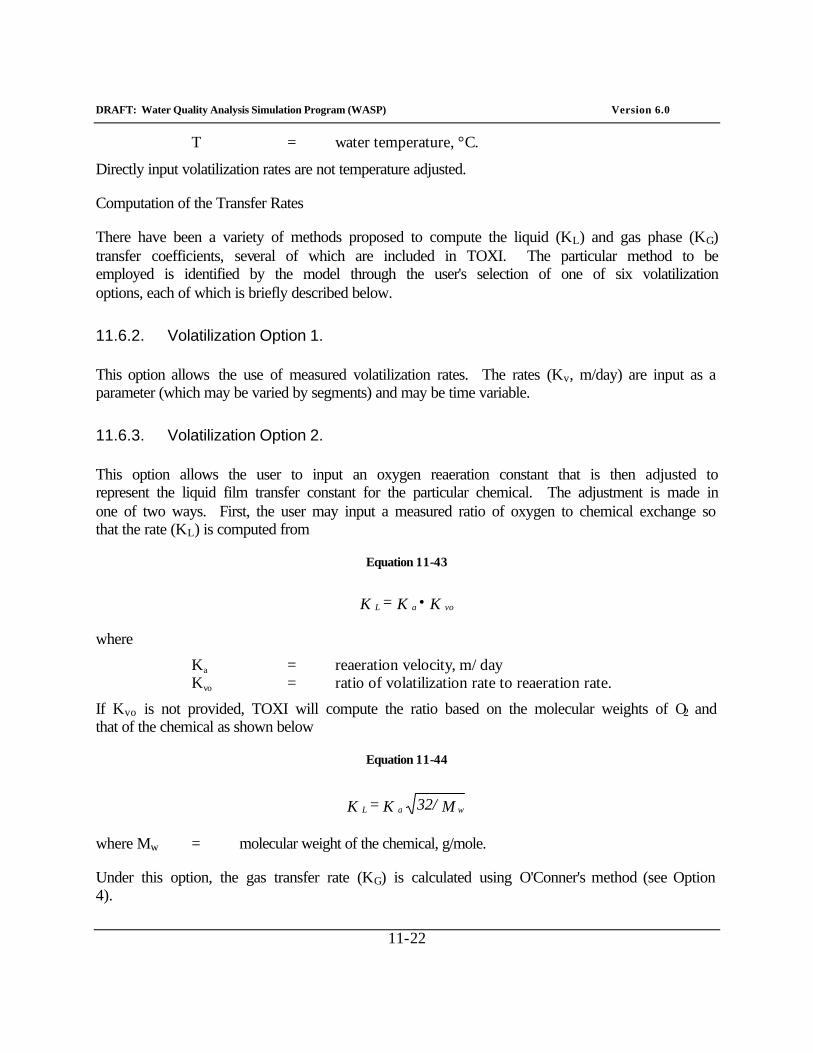
DRAFT: Water Quality Analysis Simulation Program (WASP) Version 6.0
11-22
T = water temperature, °C.
Directly input volatilization rates are not temperature adjusted.
Computation of the Transfer Rates
There have been a variety of methods proposed to compute the liquid (KL) and gas phase (KG) transfer coefficients, several of which are included in TOXI. The particular method to be employed is identified by the model through the user's selection of one of six volatilization options, each of which is briefly described below.
11.6.2. Volatilization Option 1.
This option allows the use of measured volatilization rates. The rates (Kv, m/day) are input as a parameter (which may be varied by segments) and may be time variable.
11.6.3. Volatilization Option 2.
This option allows the user to input an oxygen reaeration constant that is then adjusted to represent the liquid film transfer constant for the particular chemical. The adjustment is made in one of two ways. First, the user may input a measured ratio of oxygen to chemical exchange so that the rate (KL) is computed from
Equation 11-43
K K = K vo a L •
where
Ka = reaeration velocity, m/day Kvo = ratio of volatilization rate to reaeration rate.
If Kvo is not provided, TOXI will compute the ratio based on the molecular weights of O2 and that of the chemical as shown below
Equation 11-44
M32/ K = K wa L
where Mw = molecular weight of the chemical, g/mole.
Under this option, the gas transfer rate (KG) is calculated using O'Conner's method (see Option 4).
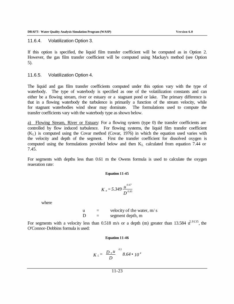
DRAFT: Water Quality Analysis Simulation Program (WASP) Version 6.0
11-23
11.6.4. Volatilization Option 3.
If this option is specified, the liquid film transfer coefficient will be computed as in Option 2. However, the gas film transfer coefficient will be computed using Mackay's method (see Option 5).
11.6.5. Volatilization Option 4.
The liquid and gas film transfer coefficients computed under this option vary with the type of waterbody. The type of waterbody is specified as one of the volatilization constants and can either be a flowing stream, river or estuary or a stagnant pond or lake. The primary difference is that in a flowing waterbody the turbulence is primarily a function of the stream velocity, while for stagnant waterbodies wind shear may dominate. The formulations used to compute the transfer coefficients vary with the waterbody type as shown below.
a) Flowing Stream, River or Estuary: For a flowing system (type 0) the transfer coefficients are controlled by flow induced turbulence. For flowing systems, the liquid film transfer coefficient (KL) is computed using the Covar method (Covar, 1976) in which the equation used varies with the velocity and depth of the segment. First the transfer coefficient for dissolved oxygen is computed using the formulations provided below and then KL calculated from equation 7.44 or 7.45.
For segments with depths less than 0.61 m the Owens formula is used to calculate the oxygen reaeration rate:
Equation 11-45
Du 5.349 = K 0.85
0.67
a
where
u = velocity of the water, m/s D = segment depth, m
For segments with a velocity less than 0.518 m/s or a depth (m) greater than 13.584 u2.9135, the O'Connor-Dobbins formula is used:
Equation 11-46
10 8.64 D
uD = K 4 w0.5
L •
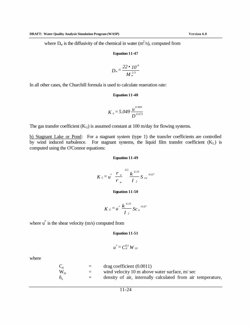
DRAFT: Water Quality Analysis Simulation Program (WASP) Version 6.0
11-24
where Dw is the diffusivity of the chemical in water (m2/s), computed from
Equation 11-47
M10 22
= D 2/3 w
-9
w•
In all other cases, the Churchill formula is used to calculate reaeration rate:
Equation 11-48
Du 5.049 = K 0.673
0.969
a
The gas transfer coefficient (KG) is assumed constant at 100 m/day for flowing systems.
b) Stagnant Lake or Pond: For a stagnant system (type 1) the transfer coefficients are controlled by wind induced turbulence. For stagnant systems, the liquid film transfer coefficient (KL) is computed using the O'Connor equations:
Equation 11-49
S u = K cw 0.67-
2
0.33
w
a
0.5
*L
λκ
ρρ
Equation 11-50
Sc u = K a 0.67-
2
0.33 *
G λ
κ
where u* is the shear velocity (m/s) computed from
Equation 11-51
W C = u 100.5d
*
where
Cd = drag coefficient (0.0011) W10 = wind velocity 10 m above water surface, m/sec ña = density of air, internally calculated from air temperature,
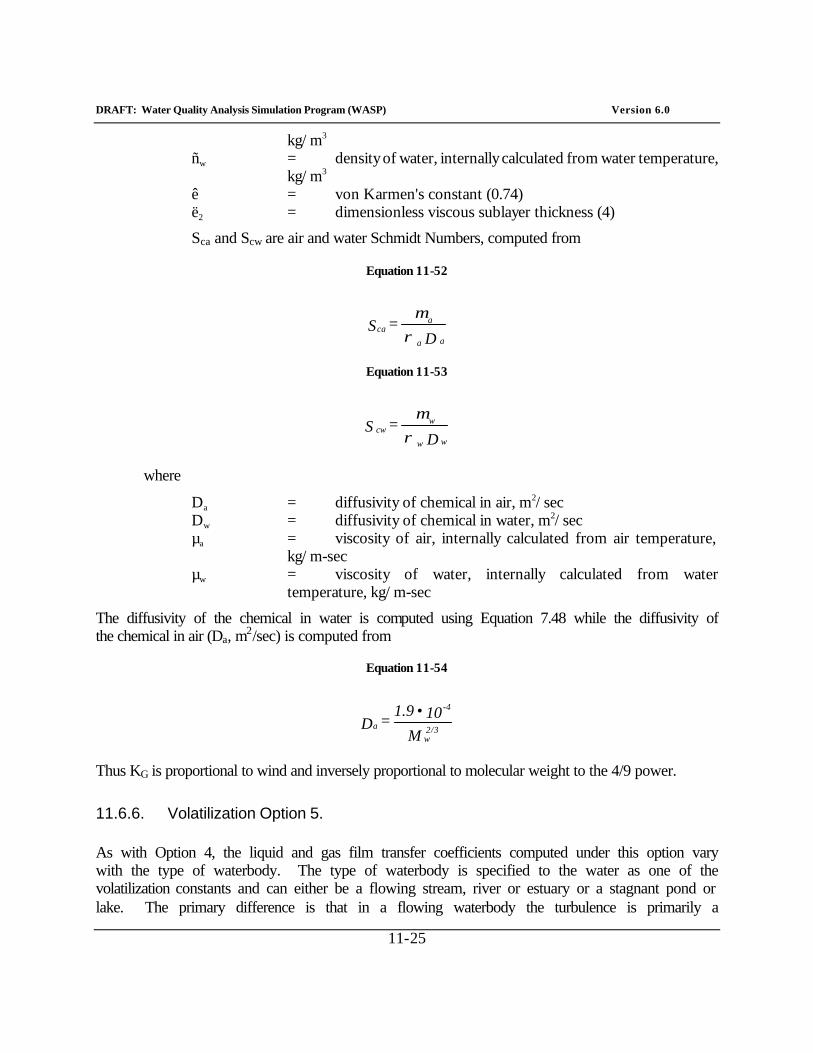
DRAFT: Water Quality Analysis Simulation Program (WASP) Version 6.0
11-25
kg/m3 ñw = density of water, internally calculated from water temperature,
kg/m3 ê = von Karmen's constant (0.74) ë2 = dimensionless viscous sublayer thickness (4)
Sca and Scw are air and water Schmidt Numbers, computed from
Equation 11-52
D = S
a a
a ca ρ
µ
Equation 11-53
D = S
w w
wcw ρ
µ
where
Da = diffusivity of chemical in air, m2/sec Dw = diffusivity of chemical in water, m2/sec µa = viscosity of air, internally calculated from air temperature,
kg/m-sec µw = viscosity of water, internally calculated from water
temperature, kg/m-sec
The diffusivity of the chemical in water is computed using Equation 7.48 while the diffusivity of the chemical in air (Da, m2/sec) is computed from
Equation 11-54
M10 1.9
= D 2/3 w
-4
a•
Thus KG is proportional to wind and inversely proportional to molecular weight to the 4/9 power.
11.6.6. Volatilization Option 5.
As with Option 4, the liquid and gas film transfer coefficients computed under this option vary with the type of waterbody. The type of waterbody is specified to the water as one of the volatilization constants and can either be a flowing stream, river or estuary or a stagnant pond or lake. The primary difference is that in a flowing waterbody the turbulence is primarily a
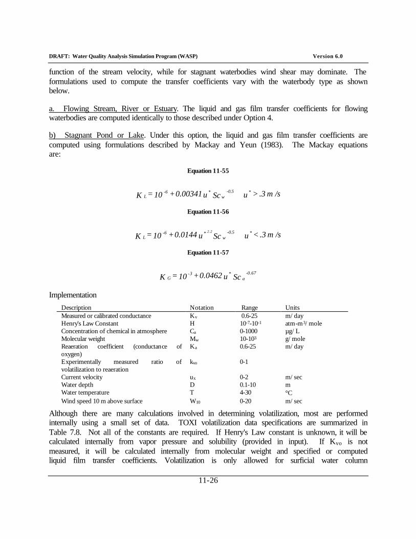
DRAFT: Water Quality Analysis Simulation Program (WASP) Version 6.0
11-26
function of the stream velocity, while for stagnant waterbodies wind shear may dominate. The formulations used to compute the transfer coefficients vary with the waterbody type as shown below.
a. Flowing Stream, River or Estuary. The liquid and gas film transfer coefficients for flowing waterbodies are computed identically to those described under Option 4.
b) Stagnant Pond or Lake. Under this option, the liquid and gas film transfer coefficients are computed using formulations described by Mackay and Yeun (1983). The Mackay equations are:
Equation 11-55
/s m .3 > u Sc u 0.00341 + 10 = K * w
0.5- * 6- L
Equation 11-56
/s m .3 < u Sc u 0.0144 + 10 = K * w
0.5- * 6- L
2.2
Equation 11-57
Sc u 0.0462 + 10 = K a 0.67- * 3-
G
Implementation
Description Notation Range Units Measured or calibrated conductance Kv 0.6-25 m/day Henry's Law Constant H 10-7-10-1 atm-m3/mole Concentration of chemical in atmosphere Ca 0-1000 µg/L Molecular weight Mw 10-103 g/mole Reaeration coefficient (conductance of oxygen)
Ka 0.6-25 m/day
Experimentally measured ratio of volatilization to reaeration
kvo 0-1
Current velocity ux 0-2 m/sec Water depth D 0.1-10 m Water temperature T 4-30 °C Wind speed 10 m above surface W10 0-20 m/sec
Although there are many calculations involved in determining volatilization, most are performed internally using a small set of data. TOXI volatilization data specifications are summarized in Table 7.8. Not all of the constants are required. If Henry's Law constant is unknown, it will be calculated internally from vapor pressure and solubility (provided in input). If Kvo is not measured, it will be calculated internally from molecular weight and specified or computed liquid film transfer coefficients. Volatilization is only allowed for surficial water column
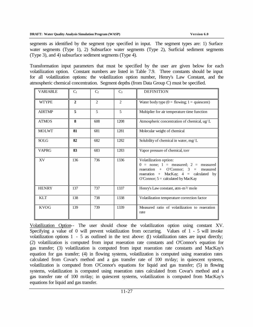
DRAFT: Water Quality Analysis Simulation Program (WASP) Version 6.0
11-27
segments as identified by the segment type specified in input. The segment types are: 1) Surface water segments (Type 1), 2) Subsurface water segments (Type 2), Surficial sediment segments (Type 3), and 4) subsurface sediment segments (Type 4).
Transformation input parameters that must be specified by the user are given below for each volatilization option. Constant numbers are listed in Table 7.9. Three constants should be input for all volatilization options: the volatilization option number, Henry's Law Constant, and the atmospheric chemical concentration. Segment depths (from Data Group C) must be specified.
VARIABLE
C1
C2
C3
DEFINITION
WTYPE
2
2
2
Water body type (0 = flowing; 1 = quiescent)
AIRTMP
5
5
5
Multiplier for air temperature time function
ATMOS
8
608
1208
Atmospheric concentration of chemical, ug/L
MOLWT
81
681
1281
Molecular weight of chemical
SOLG
82
682
1282
Solubility of chemical in water, mg/L
VAPRG
83
683
1283
Vapor pressure of chemical, torr
XV
136
736
1336
Volatilization option: 0 = none; 1 = measured; 2 = measured reaeration + O'Connor; 3 = measured reaeration + MacKay; 4 = calculated by O'Connor; 5 = calculated by MacKay
HENRY
137
737
1337
Henry's Law constant, atm-m3/mole
KLT
138
738
1338
Volatilization temperature correction factor
KVOG
139
739
1339
Measured ratio of volatilization to reaeration rate
Volatilization Option-- The user should chose the volatilization option using constant XV. Specifying a value of 0 will prevent volatilization from occurring. Values of 1 - 5 will invoke volatilization options 1 - 5 as outlined in the text above: (1) volatilization rates are input directly; (2) volatilization is computed from input reaeration rate constants and O'Connor's equation for gas transfer; (3) volatilization is computed from input reaeration rate constants and MacKay's equation for gas transfer; (4) in flowing systems, volatilization is computed using reaeration rates calculated from Covar's method and a gas transfer rate of 100 m/day; in quiescent systems, volatilization is computed from O'Connor's equations for liquid and gas transfer; (5) in flowing systems, volatilization is computed using reaeration rates calculated from Covar's method and a gas transfer rate of 100 m/day; in quiescent systems, volatilization is computed from MacKay's equations for liquid and gas transfer.
DRAFT: Water Quality Analysis Simulation Program (WASP) Version 6.0
11-28
Henry's Law Constant, atm-m3/mole-- The user should specify Henry's Law constant for air-water partitioning of the chemical using constant HENRY.
Atmospheric Concentration, ug/L-- The user should specify the mean atmospheric concentration of chemical using constant ATMOS. If this concentration is 0, then volatilization will always cause a loss of chemical from the water body.
11.6.7. Volatilization Option 1
In this option, variable volatilization rate constants can be input directly.
Volatilization Rates, m/day-- When XV is set to 1, the user may then input segment and time variable volatilization rates using parameter 5, REAR, and time function 12, REARN. The product of spatially-variable REAR and time-variable REARN gives the segment and time specific volatilization rate constants used by TOXI. These volatilization values are not modified by a temperature function.
11.6.8. Volatilization Option 2
In this option, volatilization rates are calculated from user-input reaeration rate constants and O'Connor's method for gas transfer. Input data required for option 2 are listed below. For flowing systems, wind speed and air temperature are not used and may be omitted.
Water Body Type-- The user should specify the water body type using constant WTYPE. A value of 0 indicates a flowing water body, such as a stream, river, or estuary. A value of 1 indicates a quiescent water body, such as a pond, reservoir, or lake.
Reaeration Rates, m/day-- When XV is set to 2, the user may then input segment and time variable reaeration rates using parameter 5, REAR, and time function 12, REARN. The product of spatially-variable REAR and time-variable REARN gives the segment and time specific reaeration rate constants used by TOXI. These reaeration values are not modified by a temperature function.
Ratio of Volatilization to Reaeration-- The user may specify an experimentally-measured ratio of volatilization to reaeration using constant KVOG. If this constant is not given, the ratio will be calculated from molecular weight.
Molecular Weight g/mole-- The user may specify the molecular weight using constant MOLWT. This constant is used to calculate the ratio of volatilization to reaeration if an experimentally-measured value is not provided. It is also used in the calculation of diffusivities.
Wind Speed, m/sec-- The user may specify the segment and time variable wind speed using parameter 4, WVEL, and time function 9, WINDN. The product of spatially-variable WVEL
DRAFT: Water Quality Analysis Simulation Program (WASP) Version 6.0
11-29
and time-variable WINDN gives the segment and time specific reaeration rate constants used by TOXI. Wind speed should be measured at 10 m height above the water surface.
Air Temperature, °C-- The user may specify time-variable air temperature using constant AIRTMP and time function 13, AIRTMPN. The ambient air temperature is calculated as the product of AIRTMP and AIRTMPN. For a constant air temperature, AIRTMPN can be omitted. For variable air temperatures, the user should set AIRTMP to 1.0 and input a series of air temperature versus time values via AIRTMPN.
11.6.9. Volatilization Option 3
In this option, volatilization rates are calculated from user-input reaeration rate constants and MacKay's method for gas transfer. Input data required for the same as for option 2, listed above. For flowing systems, wind speed and air temperature are not used and may be omitted.
11.6.10. Volatilization Option 4
In this option, volatilization rates in flowing systems are calculated using reaeration rates calculated from Covar's method and a gas transfer rate of 100 m/day. In quiescent systems, volatilization is computed from O'Connor's equations for liquid and gas transfer. Input data required for option 4 are listed below. For flowing systems, wind speed and air temperature are not used and may be omitted. For quiescent systems, water velocity may be omitted.
Water Velocity, m/sec-- Variable current velocities are calculated from flow using hydraulic geometry coefficients as described in Chapter 2. For most situations, no further input is required from the user. If an estuary is being simulated under tidal-average conditions, however, the net flows do not provide realistic ambient water velocities for use in volatilization calculations. In this case, the user should enter time and segment variable water velocities using parameter 1, VELFN and time functions 5-8, VELN(1-4).
The parameter VELFN indicates which velocity function will be used by the model for each segment. Values of 1.0, 2.0, 3.0, or 4.0 will call time functions VELN(1), VELN(2), VELN(3), and VELN(4), respectively. Water velocities should then be entered via these time functions as a series of velocity versus time values.
Water Body Type-- see Option 2 above.
Ratio of Volatilization to Reaeration-- see Option 2 above.
Molecular Weight g/mole-- see Option 2 above.
Wind Speed, m/sec-- see Option 2 above.
DRAFT: Water Quality Analysis Simulation Program (WASP) Version 6.0
11-30
Air Temperature, C-- see Option 2 above.
11.6.11. Volatilization Option 5
In this option, volatilization rates in flowing systems are calculated using reaeration rates calculated from Covar's method and a gas transfer rate of 100 m/day. In quiescent systems, volatilization is computed from MacKay's equations for liquid and gas transfer. Input data required for option 5 are the same as for option 4 above. For flowing systems, wind speed and air temperature are not used and may be omitted. For quiescent systems, water velocity may be omitted.
11.7. Hydrolysis
Hydrolysis, or reaction of the chemical with water, is known to be a major pathway for degradation of many toxic organics. Hydrolysis is a reaction in which cleavage of a molecular bond of the chemical and formation of a new bond with either the hydrogen or the hydroxyl component of a water molecule occurs. Hydrolytic reactions are usually catalyzed by acid and/or base and the overriding factor affecting hydrolysis rates at a given temperature is generally hydrogen or hydroxide ion concentration (Wolfe, 1980). An example reaction is shown in 8. The reaction can be catalyzed by hydrogen ions or proceed by consuming hydroxide ions. 8 illustrates the effects of base hydrolysis on carbaryl, neutral hydrolysis on chloromethane, and acid and base hydrolysis on 2,4-D.
11.7.1. Overview of TOXI Hydrolysis Reactions
Hydrolysis may be simulated by TOXI using simple decay. Alternatively, hydrolysis can be simulated using rates that are first order for the neutral chemical and second order for its ionic forms. The second order rates are pH and temperature dependant.
11.7.2. Option 1. First Order Hydrolysis.
Under this option, the user inputs a first order rate constant for either neutral, alkaline, or acid hydrolysis. The first order rate term constant is then applied to the total chemical concentration (see Section 6.3).
11.7.3. Option 2. Second Order Hydrolysis.
Under this option, hydrolysis by specific-acid-catalyzed, neutral, or base pathways is considered for the various species and phases of each chemical. The reactions are first order for the neutral chemical and second order for the acidic or basic forms of the chemical:

DRAFT: Water Quality Analysis Simulation Program (WASP) Version 6.0
11-31
Equation 11-58
f k = K ij nij ji
HN ∑∑
Equation 11-59
f] H[ k = K ij +
aij ji
HH ∑∑
Equation 11-60
f] OH[ k = K ij -
bij ji
HOH ∑∑
where:
KHN = net neutral hydrolysis rate constant, day-1 KHH = net acid catalyzed hydrolysis rate constant, day-1 KHOH = net base catalyzed hydrolysis rate constant, day-1 kaij,kbij = specific acid catalyzed and base rate constants for ionic specie
i in phase j, respectively, molar-1 day-1 knij = neutral rate constant for ionic specie i in phase j, day-1 fij = fraction of chemical as ionic specie i in phase j
The rates are also affected by temperature. TOXI adjusts the rates using the temperature-based Arrhenius function
Equation 11-61
)]T RT/( ) T - T( E [1000 )T( k = )Tk( R k R K aH R k exp
where:
TK = water temperature, °K TR = reference temperature for which reaction rate is reported, °K EaH = Arrhenius activation energy for hydrolysis reaction, kcal/mole
°K R = 1.99 cal/mole °K 1000 = cal/kcal
Implementation
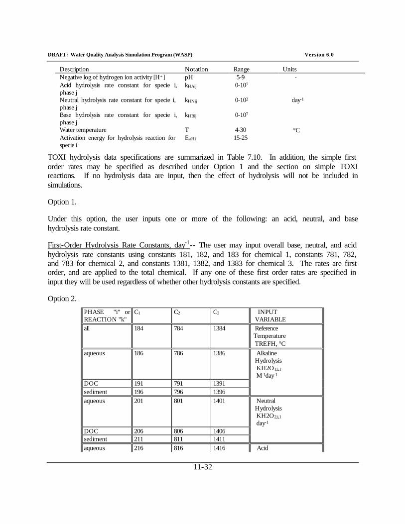
DRAFT: Water Quality Analysis Simulation Program (WASP) Version 6.0
11-32
Description Notation Range Units Negative log of hydrogen ion activity [H+] pH 5-9 - Acid hydrolysis rate constant for specie i, phase j
kHAij 0-107
Neutral hydrolysis rate constant for specie i, phase j
kHNij 0-102 day-1
Base hydrolysis rate constant for specie i, phase j
kHBij 0-107
Water temperature T 4-30 °C Activation energy for hydrolysis reaction for specie i
EaHi 15-25
TOXI hydrolysis data specifications are summarized in Table 7.10. In addition, the simple first order rates may be specified as described under Option 1 and the section on simple TOXI reactions. If no hydrolysis data are input, then the effect of hydrolysis will not be included in simulations.
Option 1.
Under this option, the user inputs one or more of the following: an acid, neutral, and base hydrolysis rate constant.
First-Order Hydrolysis Rate Constants, day-1-- The user may input overall base, neutral, and acid hydrolysis rate constants using constants 181, 182, and 183 for chemical 1, constants 781, 782, and 783 for chemical 2, and constants 1381, 1382, and 1383 for chemical 3. The rates are first order, and are applied to the total chemical. If any one of these first order rates are specified in input they will be used regardless of whether other hydrolysis constants are specified.
Option 2.
PHASE "i" or REACTION "k"
C1 C2 C3 INPUT VARIABLE
all 184 784 1384 Reference Temperature TREFH, °C
aqueous 186 786 1386 Alkaline Hydrolysis KH2O1,i,1 M-1day-1
DOC 191 791 1391 sediment 196 796 1396 aqueous 201 801 1401 Neutral
Hydrolysis KH2O2,i,1 day-1
DOC 206 806 1406 sediment 211 811 1411 aqueous 216 816 1416 Acid
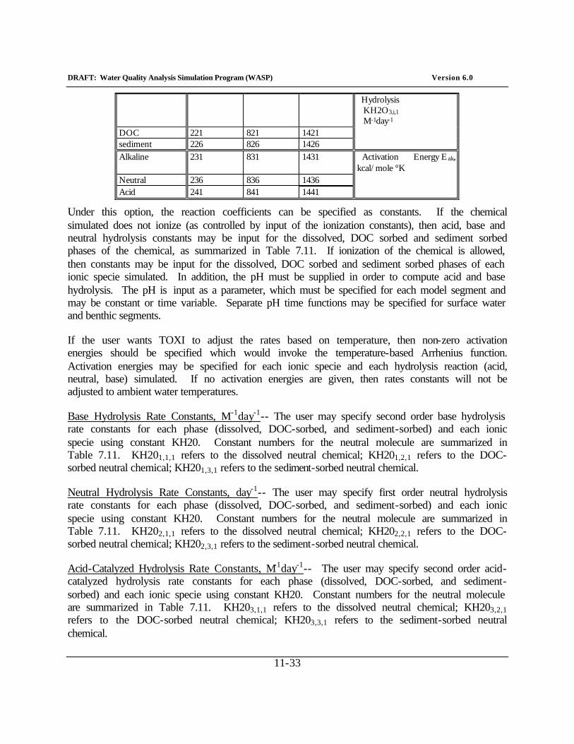
DRAFT: Water Quality Analysis Simulation Program (WASP) Version 6.0
11-33
Hydrolysis KH2O3,i,1 M-1day-1
DOC 221 821 1421 sediment 226 826 1426 Alkaline 231 831 1431 Activation Energy Eak,
kcal/mole °K Neutral 236 836 1436 Acid 241 841 1441
Under this option, the reaction coefficients can be specified as constants. If the chemical simulated does not ionize (as controlled by input of the ionization constants), then acid, base and neutral hydrolysis constants may be input for the dissolved, DOC sorbed and sediment sorbed phases of the chemical, as summarized in Table 7.11. If ionization of the chemical is allowed, then constants may be input for the dissolved, DOC sorbed and sediment sorbed phases of each ionic specie simulated. In addition, the pH must be supplied in order to compute acid and base hydrolysis. The pH is input as a parameter, which must be specified for each model segment and may be constant or time variable. Separate pH time functions may be specified for surface water and benthic segments.
If the user wants TOXI to adjust the rates based on temperature, then non-zero activation energies should be specified which would invoke the temperature-based Arrhenius function. Activation energies may be specified for each ionic specie and each hydrolysis reaction (acid, neutral, base) simulated. If no activation energies are given, then rates constants will not be adjusted to ambient water temperatures.
Base Hydrolysis Rate Constants, M-1day-1-- The user may specify second order base hydrolysis rate constants for each phase (dissolved, DOC-sorbed, and sediment-sorbed) and each ionic specie using constant KH20. Constant numbers for the neutral molecule are summarized in Table 7.11. KH201,1,1 refers to the dissolved neutral chemical; KH201,2,1 refers to the DOC-sorbed neutral chemical; KH201,3,1 refers to the sediment-sorbed neutral chemical.
Neutral Hydrolysis Rate Constants, day-1-- The user may specify first order neutral hydrolysis rate constants for each phase (dissolved, DOC-sorbed, and sediment-sorbed) and each ionic specie using constant KH20. Constant numbers for the neutral molecule are summarized in Table 7.11. KH202,1,1 refers to the dissolved neutral chemical; KH202,2,1 refers to the DOC-sorbed neutral chemical; KH202,3,1 refers to the sediment-sorbed neutral chemical.
Acid-Catalyzed Hydrolysis Rate Constants, M-1day-1-- The user may specify second order acid-catalyzed hydrolysis rate constants for each phase (dissolved, DOC-sorbed, and sediment-sorbed) and each ionic specie using constant KH20. Constant numbers for the neutral molecule are summarized in Table 7.11. KH203,1,1 refers to the dissolved neutral chemical; KH203,2,1 refers to the DOC-sorbed neutral chemical; KH203,3,1 refers to the sediment-sorbed neutral chemical.
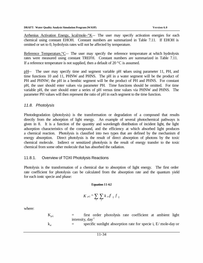
DRAFT: Water Quality Analysis Simulation Program (WASP) Version 6.0
11-34
Arrhenius Activation Energy, kcal/mole-°K-- The user may specify activation energies for each chemical using constant EHOH. Constant numbers are summarized in Table 7.11. If EHOH is omitted or set to 0, hydrolysis rates will not be affected by temperature.
Reference Temperature,°C-- The user may specify the reference temperature at which hydrolysis rates were measured using constant TREFH. Constant numbers are summarized in Table 7.11. If a reference temperature is not supplied, then a default of 20 °C is assumed.
pH-- The user may specify time and segment variable pH values using parameter 11, PH, and time functions 10 and 11, PHNW and PHNS. The pH in a water segment will be the product of PH and PHNW; the pH in a benthic segment will be the product of PH and PHNS. For constant pH, the user should enter values via parameter PH. Time functions should be omitted. For time variable pH, the user should enter a series of pH versus time values via PHNW and PHNS. The parameter PH values will then represent the ratio of pH in each segment to the time function.
11.8. Photolysis
Photodegradation (photolysis) is the transformation or degradation of a compound that results directly from the adsorption of light energy. An example of several photochemical pathways is given in 8. It is a function of the quantity and wavelength distribution of incident light, the light adsorption characteristics of the compound, and the efficiency at which absorbed light produces a chemical reaction. Photolysis is classified into two types that are defined by the mechanism of energy absorption. Direct photolysis is the result of direct absorption of photons by the toxic chemical molecule. Indirect or sensitized photolysis is the result of energy transfer to the toxic chemical from some other molecule that has absorbed the radiation.
11.8.1. Overview of TOXI Photolysis Reactions
Photolysis is the transformation of a chemical due to absorption of light energy. The first order rate coefficient for photolysis can be calculated from the absorption rate and the quantum yield for each ionic specie and phase:
Equation 11-62
f k = K ij ij ai ji
pG φ∑∑
where:
KpG = first order photolysis rate coefficient at ambient light intensity, day-1
kai = specific sunlight absorption rate for specie i, E/mole-day or
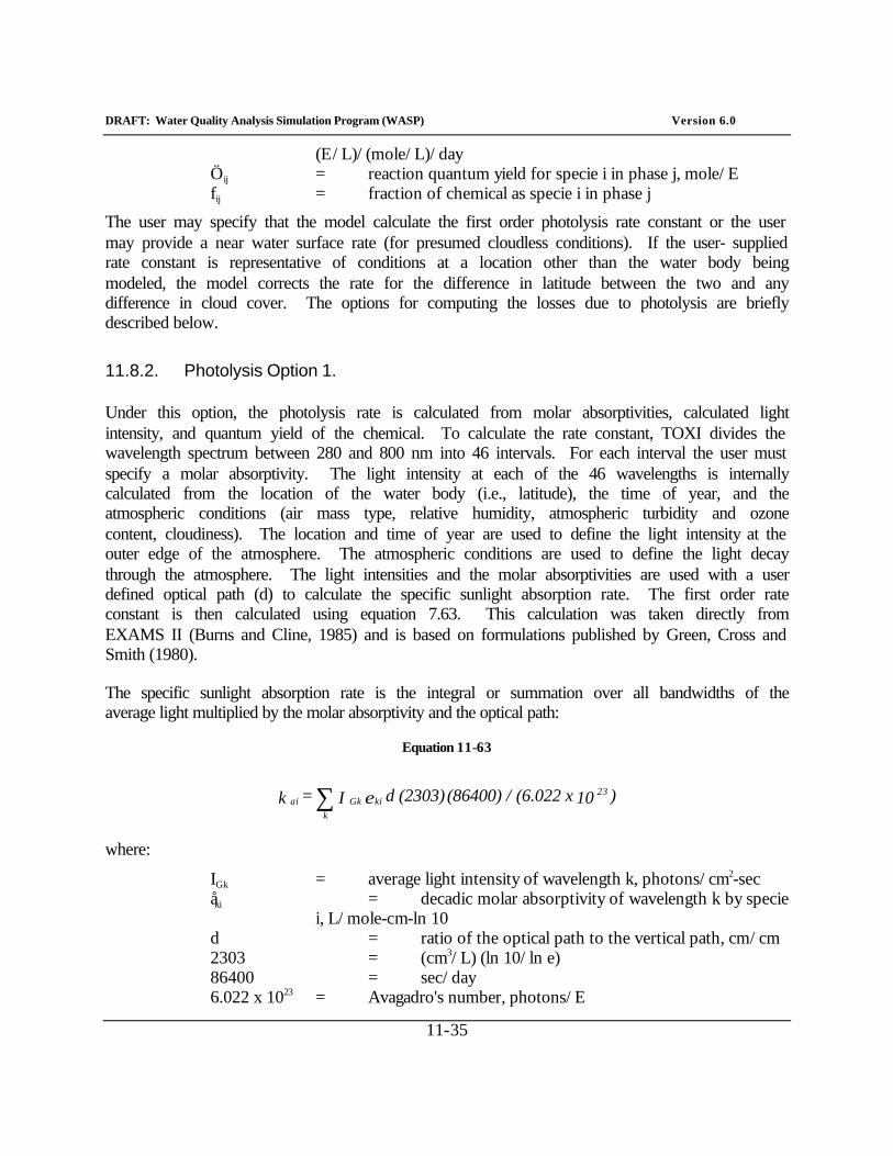
DRAFT: Water Quality Analysis Simulation Program (WASP) Version 6.0
11-35
(E/L)/(mole/L)/day Öij = reaction quantum yield for specie i in phase j, mole/E fij = fraction of chemical as specie i in phase j
The user may specify that the model calculate the first order photolysis rate constant or the user may provide a near water surface rate (for presumed cloudless conditions). If the user- supplied rate constant is representative of conditions at a location other than the water body being modeled, the model corrects the rate for the difference in latitude between the two and any difference in cloud cover. The options for computing the losses due to photolysis are briefly described below.
11.8.2. Photolysis Option 1.
Under this option, the photolysis rate is calculated from molar absorptivities, calculated light intensity, and quantum yield of the chemical. To calculate the rate constant, TOXI divides the wavelength spectrum between 280 and 800 nm into 46 intervals. For each interval the user must specify a molar absorptivity. The light intensity at each of the 46 wavelengths is internally calculated from the location of the water body (i.e., latitude), the time of year, and the atmospheric conditions (air mass type, relative humidity, atmospheric turbidity and ozone content, cloudiness). The location and time of year are used to define the light intensity at the outer edge of the atmosphere. The atmospheric conditions are used to define the light decay through the atmosphere. The light intensities and the molar absorptivities are used with a user defined optical path (d) to calculate the specific sunlight absorption rate. The first order rate constant is then calculated using equation 7.63. This calculation was taken directly from EXAMS II (Burns and Cline, 1985) and is based on formulations published by Green, Cross and Smith (1980).
The specific sunlight absorption rate is the integral or summation over all bandwidths of the average light multiplied by the molar absorptivity and the optical path:
Equation 11-63
)10 x (6.022 / (86400) (2303) d I = k 23 kiGk
kai ε∑
where:
IGk = average light intensity of wavelength k, photons/cm2-sec åki = decadic molar absorptivity of wavelength k by specie
i, L/mole-cm-ln 10 d = ratio of the optical path to the vertical path, cm/cm 2303 = (cm3/L) (ln 10/ln e) 86400 = sec/day 6.022 x 1023 = Avagadro's number, photons/E
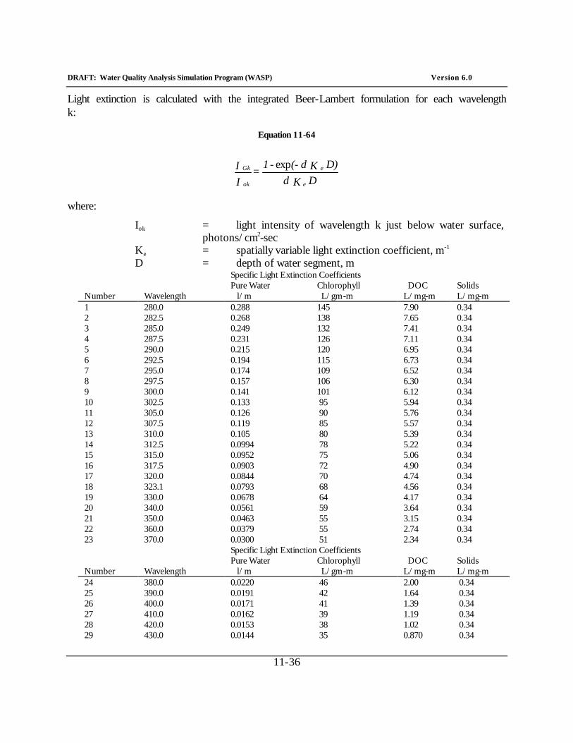
DRAFT: Water Quality Analysis Simulation Program (WASP) Version 6.0
11-36
Light extinction is calculated with the integrated Beer-Lambert formulation for each wavelength k:
Equation 11-64
D K dD) K d (- - 1
= II
e
e
ok
Gk exp
where:
Iok = light intensity of wavelength k just below water surface, photons/cm2-sec
Ke = spatially variable light extinction coefficient, m-1 D = depth of water segment, m
Specific Light Extinction Coefficients Number
Wavelength
Pure Water l/m
Chlorophyll L/gm-m
DOC L/mg-m
Solids L/mg-m
1 280.0 0.288 145 7.90 0.34 2 282.5 0.268 138 7.65 0.34 3 285.0 0.249 132 7.41 0.34 4 287.5 0.231 126 7.11 0.34 5 290.0 0.215 120 6.95 0.34 6 292.5 0.194 115 6.73 0.34 7 295.0 0.174 109 6.52 0.34 8 297.5 0.157 106 6.30 0.34 9 300.0 0.141 101 6.12 0.34 10 302.5 0.133 95 5.94 0.34 11 305.0 0.126 90 5.76 0.34 12 307.5 0.119 85 5.57 0.34 13 310.0 0.105 80 5.39 0.34 14 312.5 0.0994 78 5.22 0.34 15 315.0 0.0952 75 5.06 0.34 16 317.5 0.0903 72 4.90 0.34 17 320.0 0.0844 70 4.74 0.34 18 323.1 0.0793 68 4.56 0.34 19 330.0 0.0678 64 4.17 0.34 20 340.0 0.0561 59 3.64 0.34 21 350.0 0.0463 55 3.15 0.34 22 360.0 0.0379 55 2.74 0.34 23 370.0 0.0300 51 2.34 0.34 Specific Light Extinction Coefficients Number
Wavelength
Pure Water l/m
Chlorophyll L/gm-m
DOC L/mg-m
Solids L/mg-m
24 380.0 0.0220 46 2.00 0.34 25 390.0 0.0191 42 1.64 0.34 26 400.0 0.0171 41 1.39 0.34 27 410.0 0.0162 39 1.19 0.34 28 420.0 0.0153 38 1.02 0.34 29 430.0 0.0144 35 0.870 0.34

DRAFT: Water Quality Analysis Simulation Program (WASP) Version 6.0
11-37
Specific Light Extinction Coefficients Number
Wavelength
Pure Water l/m
Chlorophyll L/gm-m
DOC L/mg-m
Solids L/mg-m
1 280.0 0.288 145 7.90 0.34 30 440.0 0.0145 32 0.753 0.34 31 450.0 0.0145 31 0.654 0.34 32 460.0 0.0156 28 0.573 0.34 33 470.0 0.0156 26 0.504 0.34 34 480.0 0.0176 24 0.444 0.34 35 490.0 0.0196 22 0.396 0.34 36 503.75 0.0295 19 0.357 0.34 37 525.0 0.0492 14 0.282 0.34 38 550.0 0.0638 10 0.228 0.34 39 575.0 0.0940 8 0.188 0.34 40 600.0 0.244 6 0.158 0.34 41 625.0 0.314 5 0.0 0.34 42 650.0 0.349 8 0.0 0.34 43 675.0 0.440 13 0.0 0.34 44 706.25 0.768 3 0.0 0.34 45 750.0 2.47 2 0.0 0.34 46 800.0 2.07 0 0.0 0.34
Iok is calculated for each wavelength based upon the time of year, latitude, ground elevation, cloud cover, air mass type, relative humidity, atmospheric turbidity, and ozone content. The atmospheric characteristics can vary monthly, or be specified as an annual average. The value of d, the ratio of the optical path to the vertical depth is difficult to compute, but a probable best value is 1.19 (Hutchinson, 1967). However, in the presence of a large concentration of scattering particles, it may approach 2.0. In order to ensure that an improper value is not loaded and used in computations, the input value is checked and set to 1.19 if the input is invalid.
The photolysis rate constants for each water column segment are determined from the calculated near-surface rate constant and the rate of light decay in the water column (Ke). The value of Ke is calculated for each wavelength based on a formulation taken from EXAMS II:
Equation 11-65
m + DOC + CHL + K = K 3 2 1 ew e ηηη
where
Kew = pure water extinction coefficient, 1/m CHL = phytoplankton chlorophyll concentration, mg/L DOC = dissolved organic carbon concentration, mg/L m = solids concentration, mg/L ç1,ç2,ç3 = specific extinction coefficients, L/mg-m
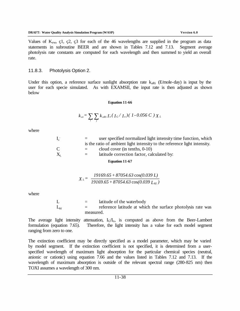
DRAFT: Water Quality Analysis Simulation Program (WASP) Version 6.0
11-38
Values of Kew, ç1, ç2, ç3 for each of the 46 wavelengths are supplied in the program as data statements in subroutine BEER and are shown in Tables 7.12 and 7.13. Segment average photolysis rate constants are computed for each wavelength and then summed to yield an overall rate.
11.8.3. Photolysis Option 2.
Under this option, a reference surface sunlight absorption rate kaRi (E/mole-day) is input by the user for each specie simulated. As with EXAMSII, the input rate is then adjusted as shown below
Equation 11-66
X ) C 0.056 - 1 ( )I/I( I k = k LoG,oaRi
jiai ∑∑
where
Io, = user specified normalized light intensity time function, which
is the ratio of ambient light intensity to the reference light intensity. C = cloud cover (in tenths, 0-10) XL = latitude correction factor, calculated by:
Equation 11-67
)L (0.039 87054.63 + 19169.65
L) (0.039 87054.63 + 19169.65 = X
RfL
coscos
where
L = latitude of the waterbody LRf = reference latitude at which the surface photolysis rate was
measured.
The average light intensity attenuation, IG/Io, is computed as above from the Beer-Lambert formulation (equation 7.65). Therefore, the light intensity has a value for each model segment ranging from zero to one.
The extinction coefficient may be directly specified as a model parameter, which may be varied by model segment. If the extinction coefficient is not specified, it is determined from a user-specified wavelength of maximum light absorption for the particular chemical species (neutral, anionic or cationic) using equation 7.66 and the values listed in Tables 7.12 and 7.13. If the wavelength of maximum absorption is outside of the relevant spectral range (280-825 nm) then TOXI assumes a wavelength of 300 nm.
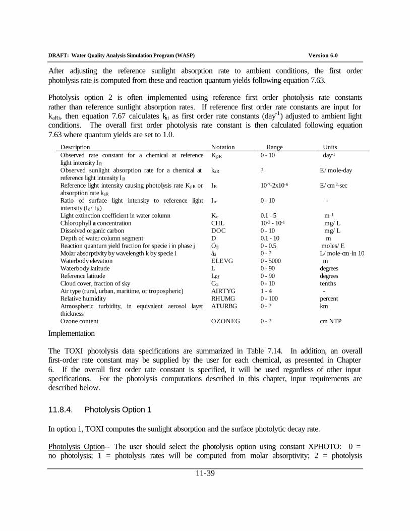
DRAFT: Water Quality Analysis Simulation Program (WASP) Version 6.0
11-39
After adjusting the reference sunlight absorption rate to ambient conditions, the first order photolysis rate is computed from these and reaction quantum yields following equation 7.63.
Photolysis option 2 is often implemented using reference first order photolysis rate constants rather than reference sunlight absorption rates. If reference first order rate constants are input for kaRi, then equation 7.67 calculates kai as first order rate constants (day-1) adjusted to ambient light conditions. The overall first order photolysis rate constant is then calculated following equation 7.63 where quantum yields are set to 1.0.
Description Notation Range Units Observed rate constant for a chemical at reference light intensity IR
KpR 0 - 10 day-1
Observed sunlight absorption rate for a chemical at reference light intensity IR
kaR ? E/mole-day
Reference light intensity causing photolysis rate KpR or absorption rate kaR
IR 10-7-2x10⁻⁶ E/cm 2-sec
Ratio of surface light intensity to reference light intensity (Io/IR)
Io, 0 - 10 -
Light extinction coefficient in water column Ke 0.1 - 5 m -1 Chlorophyll a concentration CHL 10-3 - 10-1 mg/L Dissolved organic carbon DOC 0 - 10 mg/L Depth of water column segment D 0.1 - 10 m Reaction quantum yield fraction for specie i in phase j Öij 0 - 0.5 moles/E Molar absorptivity by wavelength k by specie i åki 0 - ? L/mole-cm-ln 10 Waterbody elevation ELEVG 0 - 5000 m Waterbody latitude L 0 - 90 degrees Reference latitude LRf 0 - 90 degrees Cloud cover, fraction of sky CG 0 - 10 tenths Air type (rural, urban, maritime, or tropospheric) AIRTYG 1 - 4 - Relative humidity RHUMG 0 - 100 percent Atmospheric turbidity, in equivalent aerosol layer thickness
ATURBG 0 - ? km
Ozone content OZONEG 0 - ? cm NTP
Implementation
The TOXI photolysis data specifications are summarized in Table 7.14. In addition, an overall first-order rate constant may be supplied by the user for each chemical, as presented in Chapter 6. If the overall first order rate constant is specified, it will be used regardless of other input specifications. For the photolysis computations described in this chapter, input requirements are described below.
11.8.4. Photolysis Option 1
In option 1, TOXI computes the sunlight absorption and the surface photolytic decay rate.
Photolysis Option-- The user should select the photolysis option using constant XPHOTO: 0 = no photolysis; 1 = photolysis rates will be computed from molar absorptivity; 2 = photolysis
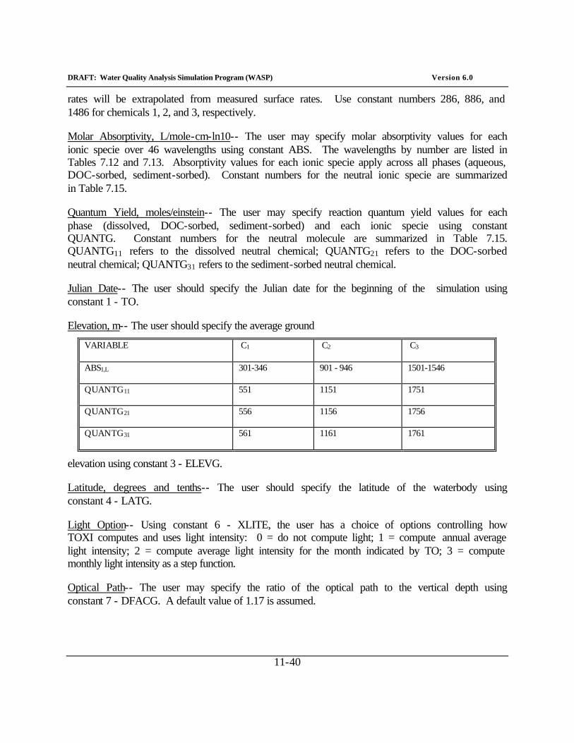
DRAFT: Water Quality Analysis Simulation Program (WASP) Version 6.0
11-40
rates will be extrapolated from measured surface rates. Use constant numbers 286, 886, and 1486 for chemicals 1, 2, and 3, respectively.
Molar Absorptivity, L/mole-cm-ln10-- The user may specify molar absorptivity values for each ionic specie over 46 wavelengths using constant ABS. The wavelengths by number are listed in Tables 7.12 and 7.13. Absorptivity values for each ionic specie apply across all phases (aqueous, DOC-sorbed, sediment-sorbed). Constant numbers for the neutral ionic specie are summarized in Table 7.15.
Quantum Yield, moles/einstein-- The user may specify reaction quantum yield values for each phase (dissolved, DOC-sorbed, sediment-sorbed) and each ionic specie using constant QUANTG. Constant numbers for the neutral molecule are summarized in Table 7.15. QUANTG11 refers to the dissolved neutral chemical; QUANTG21 refers to the DOC-sorbed neutral chemical; QUANTG31 refers to the sediment-sorbed neutral chemical.
Julian Date-- The user should specify the Julian date for the beginning of the simulation using constant 1 - TO.
Elevation, m-- The user should specify the average ground
VARIABLE
C1
C2
C3
ABS1,L
301-346
901 - 946
1501-1546
QUANTG11
551
1151
1751
QUANTG21
556
1156
1756
QUANTG31
561
1161
1761
elevation using constant 3 - ELEVG.
Latitude, degrees and tenths-- The user should specify the latitude of the waterbody using constant 4 - LATG.
Light Option-- Using constant 6 - XLITE, the user has a choice of options controlling how TOXI computes and uses light intensity: 0 = do not compute light; 1 = compute annual average light intensity; 2 = compute average light intensity for the month indicated by TO; 3 = compute monthly light intensity as a step function.
Optical Path-- The user may specify the ratio of the optical path to the vertical depth using constant 7 - DFACG. A default value of 1.17 is assumed.
DRAFT: Water Quality Analysis Simulation Program (WASP) Version 6.0
11-41
Cloud Cover, tenths-- The user should specify the mean monthly or annual average cloud cover using constant CLOUDG. Monthly values can be entered using constant numbers 11-22; the annual average can be entered using number 23.
Air Type-- The user should specify the mean air mass type using constant AIRTYG. Values of 1, 2, 3, or 4 will select rural, urban, maritime, or tropospheric, respectively. Monthly values can be entered using constant numbers 24-35; the annual average can be entered using number 36.
Relative Humidity, percent-- The user should specify the mean monthly daylight relative humidity using constant RHUMG. Monthly values can be entered using constant numbers 37-48; the annual average can be entered using number 49.
Atmospheric Turbidity, km-- The user should specify the mean atmospheric turbidity (in equivalent aerosol layer thickness, km) using constant ATURBG. Monthly values can be entered using constant numbers 50-61; the annual average can be entered using number 62.
Ozone Content, cm NTP-- The user should specify the mean ozone content (cm NTP) using constant OZONEG. Monthly values can be entered using constant numbers 63-74; the annual average can be entered using number 75.
Dissolved Organic Carbon, mg/L-- The user may specify segment variable dissolved organic carbon concentrations using parameter 6 - DOC. (Group G, Record 4, PARAM(I,6))
Chlorophyll a, mg/L-- Time and segment variable phytoplankton chlorophyll a concentrations can be specified using parameter 10, CHPHL and time function 14, CHLN. If chlorophyll concentrations are to remain constant in time, the user should enter segment mean concentrations using parameter CHPHL. CHLN should be omitted.
The user may enter time-variable chlorophyll a concentrations via time function CHLN as a series of concentration versus time values. Parameter CHPHL will then represent the ratio of each segment concentration to the time function values. The product of CHPHL and the CHLN function gives the segment and time specific chlorophyll concentrations used by TOXI. (Group G, Record 4, PARAM(I,10); Group I, Record 2, VALT(14,K)
11.8.5. Photolysis Option 2
In option 2, TOXI extrapolates either observed sunlight absorption rates or photolytic decay rates under "reference" conditions to ambient conditions. Required input data are described below.
Photolysis Option-- The user should select the photolysis option using constant XPHOTO: 0 = no photolysis; 1 = photolysis rates will be computed from molar absorptivity; 2 = photolysis rates will be extrapolated from measured surface rates. Use constant numbers 286, 886, and 1486 for chemicals 1, 2, and 3, respectively.
DRAFT: Water Quality Analysis Simulation Program (WASP) Version 6.0
11-42
Measured Photolysis Rate, day-1-- The user may specify the measured photolysis rate constant under reference conditions using constant KDPG. Values for the neutral molecule of chemicals 1, 2, and 3 can be entered using constants 291, 891, and 1491, respectively. Separate values can be entered for each ionic specie. If a reference first order rate constant is input, the quantum yield should be set to 1.0.
Measured Sunlight Absorption Rate, einstein/mole-day-- The user may specify measured sunlight absorption rates under reference conditions using constant KDPG. Values for the neutral molecule of chemicals 1, 2, and 3 can be entered using constants 291, 891, and 1491, respectively. Separate values can be entered for each ionic specie. If a reference sunlight absorption rate is input, the corresponding quantum yield must be specified.
Quantum Yield, moles/einstein-- The user may specify reaction quantum yield values for each phase (dissolved, DOC-sorbed, sediment-sorbed) and each ionic specie using constant QUANTG. Constant numbers for the neutral molecule are summarized in Table 7.15. QUANTG11 refers to the dissolved neutral chemical; QUANTG21 refers to the DOC-sorbed neutral chemical; QUANTG31 refers to the sediment-sorbed neutral chemical. Separate values can be entered for each ionic specie.
Reference Latitude, degree and tenths-- The user may specify the latitude at which the reference surface water photolytic rates were measured using constant RFLATG. Values for chemicals 1, 2, and 3 can be entered using constant numbers 288, 888, and 1488, respectively.
Maximum Absorption Wavelength, nm-- The user should specify the wavelength of maximum absorption using constant LAMAXG. Values for the neutral specie of chemicals 1, 2, and 3 can be entered using constants 296, 896, and 1496, respectively. Separate values can be entered for each ionic specie.
Latitude, degrees and tenths-- The user should specify the latitude of the waterbody using constant 4 - LATG.
Cloud Cover, tenths-- The user should specify the mean monthly or annual average cloud cover using constant CLOUDG. Monthly values can be entered using constant numbers 11-22; the annual average can be entered using number 23.
Light Intensity-- The user can specify time-variable normalized light intensity (dimensionless) using time function 15, PHTON. This function is used to adjust the measured rate constant under controlled reference light intensity to a predicted rate constant under ambient light intensity. The default value for this function is 1.0.
Light Extinction Coefficient, m-1-- The user can specify segment light extinction coefficients for the photochemically active light using parameter 12, XKE2. When this number is zero, the extinction coefficients are calculated from solids, DOC and chlorophyll a concentrations for the wavelength of maximum absorption. DOC and chlorophyll a are specified as model parameters
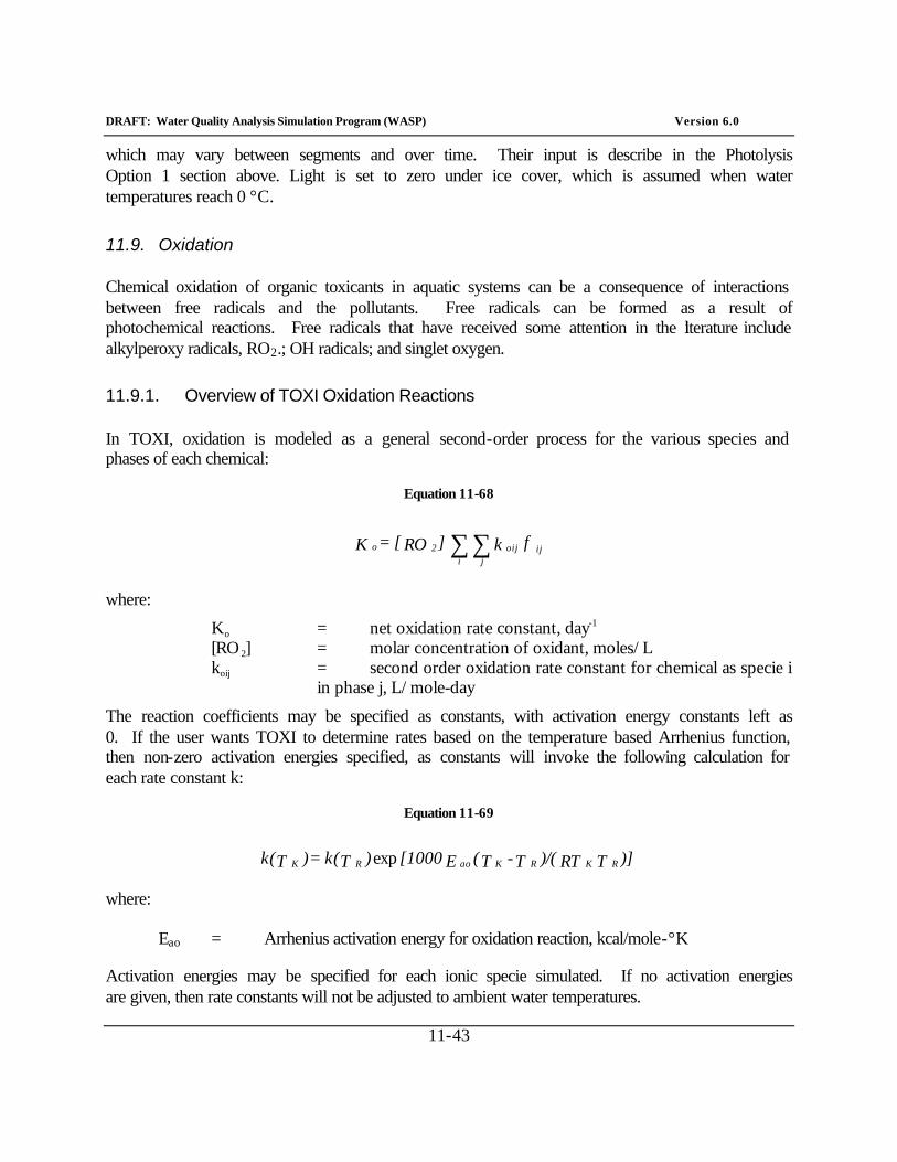
DRAFT: Water Quality Analysis Simulation Program (WASP) Version 6.0
11-43
which may vary between segments and over time. Their input is describe in the Photolysis Option 1 section above. Light is set to zero under ice cover, which is assumed when water temperatures reach 0 °C.
11.9. Oxidation
Chemical oxidation of organic toxicants in aquatic systems can be a consequence of interactions between free radicals and the pollutants. Free radicals can be formed as a result of photochemical reactions. Free radicals that have received some attention in the literature include alkylperoxy radicals, RO2.; OH radicals; and singlet oxygen.
11.9.1. Overview of TOXI Oxidation Reactions
In TOXI, oxidation is modeled as a general second-order process for the various species and phases of each chemical:
Equation 11-68
f k ] RO[ = K ij oij ji
2 o ∑∑
where:
Ko = net oxidation rate constant, day-1 [RO2] = molar concentration of oxidant, moles/L koij = second order oxidation rate constant for chemical as specie i
in phase j, L/mole-day
The reaction coefficients may be specified as constants, with activation energy constants left as 0. If the user wants TOXI to determine rates based on the temperature based Arrhenius function, then non-zero activation energies specified, as constants will invoke the following calculation for each rate constant k:
Equation 11-69
)]T RT)/(T - T( E [1000 )Tk( = )Tk( R K R K ao R K exp
where:
Eao = Arrhenius activation energy for oxidation reaction, kcal/mole-°K
Activation energies may be specified for each ionic specie simulated. If no activation energies are given, then rate constants will not be adjusted to ambient water temperatures.
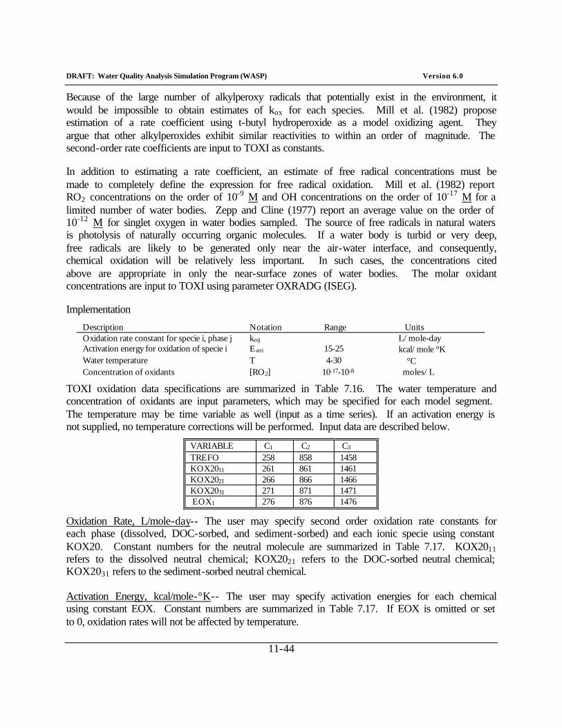
DRAFT: Water Quality Analysis Simulation Program (WASP) Version 6.0
11-44
Because of the large number of alkylperoxy radicals that potentially exist in the environment, it would be impossible to obtain estimates of kox for each species. Mill et al. (1982) propose estimation of a rate coefficient using t-butyl hydroperoxide as a model oxidizing agent. They argue that other alkylperoxides exhibit similar reactivities to within an order of magnitude. The second-order rate coefficients are input to TOXI as constants.
In addition to estimating a rate coefficient, an estimate of free radical concentrations must be made to completely define the expression for free radical oxidation. Mill et al. (1982) report RO2 concentrations on the order of 10-9 M and OH concentrations on the order of 10-17 M for a limited number of water bodies. Zepp and Cline (1977) report an average value on the order of 10-12 M for singlet oxygen in water bodies sampled. The source of free radicals in natural waters is photolysis of naturally occurring organic molecules. If a water body is turbid or very deep, free radicals are likely to be generated only near the air-water interface, and consequently, chemical oxidation will be relatively less important. In such cases, the concentrations cited above are appropriate in only the near-surface zones of water bodies. The molar oxidant concentrations are input to TOXI using parameter OXRADG (ISEG).
Implementation
Description Notation Range Units Oxidation rate constant for specie i, phase j koij L/mole-day Activation energy for oxidation of specie i Eaoi 15-25 kcal/mole °K Water temperature T 4-30 °C Concentration of oxidants [RO2] 10-17-10-8 moles/L
TOXI oxidation data specifications are summarized in Table 7.16. The water temperature and concentration of oxidants are input parameters, which may be specified for each model segment. The temperature may be time variable as well (input as a time series). If an activation energy is not supplied, no temperature corrections will be performed. Input data are described below.
VARIABLE C1 C2 C3 TREFO 258 858 1458 KOX2011 261 861 1461 KOX2021 266 866 1466 KOX2031 271 871 1471 EOX1 276 876 1476
Oxidation Rate, L/mole-day-- The user may specify second order oxidation rate constants for each phase (dissolved, DOC-sorbed, and sediment-sorbed) and each ionic specie using constant KOX20. Constant numbers for the neutral molecule are summarized in Table 7.17. KOX2011 refers to the dissolved neutral chemical; KOX2021 refers to the DOC-sorbed neutral chemical; KOX2031 refers to the sediment-sorbed neutral chemical.
Activation Energy, kcal/mole-°K-- The user may specify activation energies for each chemical using constant EOX. Constant numbers are summarized in Table 7.17. If EOX is omitted or set to 0, oxidation rates will not be affected by temperature.
DRAFT: Water Quality Analysis Simulation Program (WASP) Version 6.0
11-45
Reference Temperature,°C-- The user may specify the reference temperature at which oxidation rates were measured using constant TREFO. Constant numbers are summarized in Table 7.17. If a reference temperature is not supplied, then a default of 20 °C is assumed.
Oxidant Concentration, mole/L-- The user should specify segment variable oxidant concentrations using parameter 13, OXRAD. (Group G, Record 4, PARAM(I,13)
11.10. Biodegradation
Bacterial degradation, sometimes referred to as microbial transformation, biodegradation or biolysis, is the breakdown of a compound by the enzyme systems in bacteria. Examples are given in 8. Although these transformations can detoxify and mineralize toxins and defuse potential toxins, they can also activate potential toxins.
Biodegradation encompasses the broad and complex processes of enzymatic attack by organisms on organic chemicals. Bacteria, and to a lesser extent fungi, are the mediators of biological degradation in surface water systems. Dehalogenation, dealkylation, hydrolysis, oxidation, reduction, ring cleavage, and condensation reactions are all known to occur either metabolically or via organisms that are not capable of utilizing the chemical as a substrate for growth.
Two general types of biodegradation are recognized--growth metabolism and cometabolism. Growth metabolism occurs when the organic compound serves as a food source for the bacteria. Adaptation times from 2 to 20 days were suggested in Mills et al., 1985. Adaptation may not be required for some chemicals or in chronically exposed environments. Adaptation times may be lengthy in environments with a low initial density of degraders (Mills et al., 1985). For cases where biodegradation is limited by the degrader population size, adaptation is faster for high initial microbial populations and slower for low initial populations. Following adaptation, biodegradation proceeds at fast first-order rates. Cometabolism occurs when the organic compound is not a food source for the bacteria. Adaptation is seldom necessary, and the transformation rates are slow compared with growth metabolism.
The growth kinetics of the bacterial population degrading a toxic chemical are not well understood. The presence of competing substrates and of other bacteria, the toxicity of the chemical to the degrading bacteria, and the possibilities of adaptation to the chemical or co-metabolism make quantification of changes in the population difficult. As a result, toxic chemical models assume a constant biological activity rather than modeling the bacteria directly. Often, measured first order biodegradation rate constants from other aquatic systems are used directly.

DRAFT: Water Quality Analysis Simulation Program (WASP) Version 6.0
11-46
11.10.1. Overview of TOXI Biodegradation Reactions
In TOXI, first order biodegradation rate constants or half lives for the water column and the benthos may be specified. If these rate constants have been measured under similar conditions, this first order approach is likely to be as accurate as more complicated approaches. If first order rates are unavailable, or if they must be extrapolated to different bacterial conditions, then the second-order approach may be used. It is assumed that bacterial populations are unaffected by the presence of the compound at low concentrations. Second-order kinetics for dissolved, DOC-sorbed, and sediment-sorbed chemical are considered:
Equation 11-70
1,2 =j f k (t) P = K ij Bij ji
bac Bw ∑∑
Equation 11-71
3 =j f k (t) P = K ij Bij ji
bac Bs ∑∑
where:
KBw = net biodegradation rate constant in water, day-1 KBs = net biodegradation rate constant on sediment, day-1
kBij = second order biodegradation rate constant for specie i, phase j, ml/cell-day
Pbac(t) = active bacterial population density in segment, cell/ml fij = fraction of chemical as specie i in phase j
In TOXI, the biodegradation rate may be adjusted by temperature as shown below
Equation 11-72
Q k = (T) k20)/10-(T
Tij Bij Bij
where:
QTij = "Q-10" temperature correction factor for biodegradation of specie i, phase j
T = ambient temperature in segment, °C
The temperature correction factors represent the increase in the biodegradation rate constants resulting from a 10°C temperature increase. Values in the range of 1.5 to 2 are common.
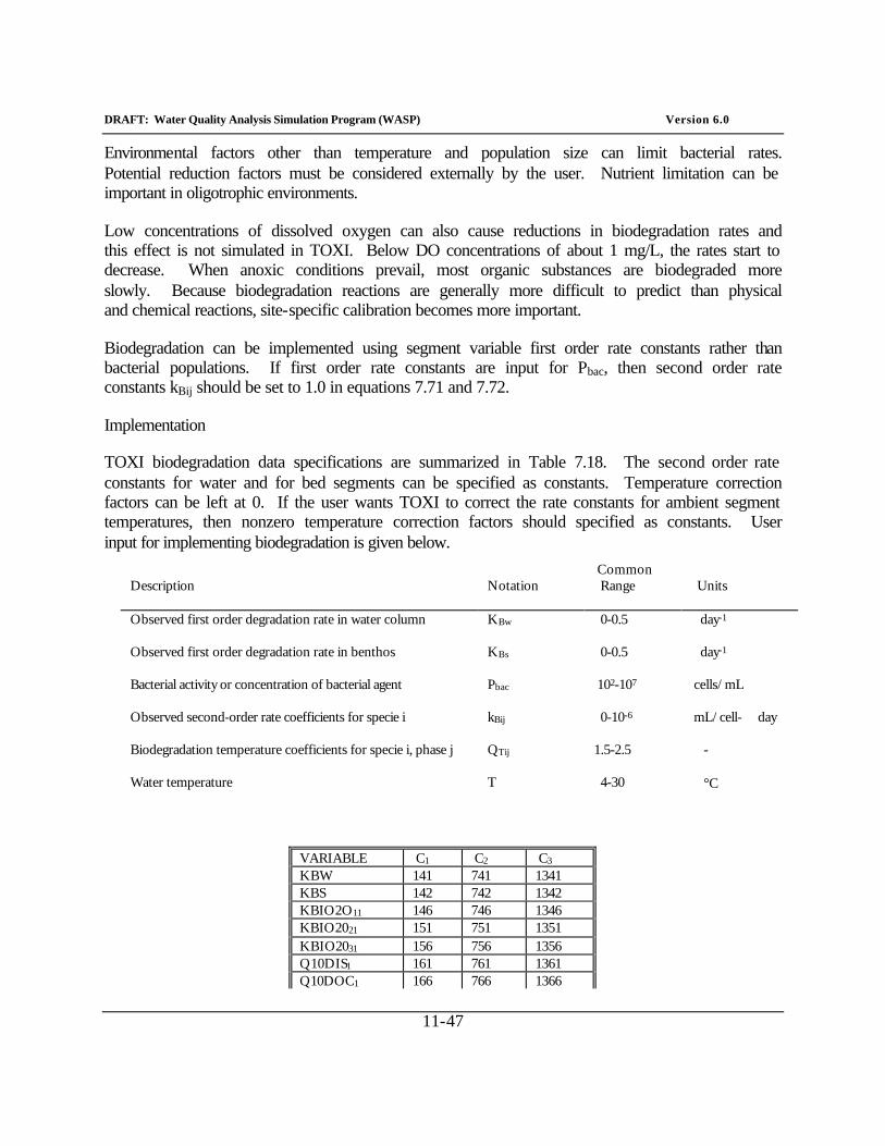
DRAFT: Water Quality Analysis Simulation Program (WASP) Version 6.0
11-47
Environmental factors other than temperature and population size can limit bacterial rates. Potential reduction factors must be considered externally by the user. Nutrient limitation can be important in oligotrophic environments.
Low concentrations of dissolved oxygen can also cause reductions in biodegradation rates and this effect is not simulated in TOXI. Below DO concentrations of about 1 mg/L, the rates start to decrease. When anoxic conditions prevail, most organic substances are biodegraded more slowly. Because biodegradation reactions are generally more difficult to predict than physical and chemical reactions, site-specific calibration becomes more important.
Biodegradation can be implemented using segment variable first order rate constants rather than bacterial populations. If first order rate constants are input for Pbac, then second order rate constants kBij should be set to 1.0 in equations 7.71 and 7.72.
Implementation
TOXI biodegradation data specifications are summarized in Table 7.18. The second order rate constants for water and for bed segments can be specified as constants. Temperature correction factors can be left at 0. If the user wants TOXI to correct the rate constants for ambient segment temperatures, then nonzero temperature correction factors should specified as constants. User input for implementing biodegradation is given below.
Description
Notation
Common Range
Units
Observed first order degradation rate in water column
KBw
0-0.5
day-1
Observed first order degradation rate in benthos
KBs
0-0.5
day-1
Bacterial activity or concentration of bacterial agent
Pbac
102-107
cells/mL
Observed second-order rate coefficients for specie i
kBij
0-10-6
mL/cell- day
Biodegradation temperature coefficients for specie i, phase j
QTij
1.5-2.5
-
Water temperature
T
4-30
°C
VARIABLE C1 C2 C3 KBW 141 741 1341 KBS 142 742 1342 KBIO2O11 146 746 1346 KBIO2021 151 751 1351 KBIO2031 156 756 1356 Q10DIS1 161 761 1361 Q10DOC1 166 766 1366
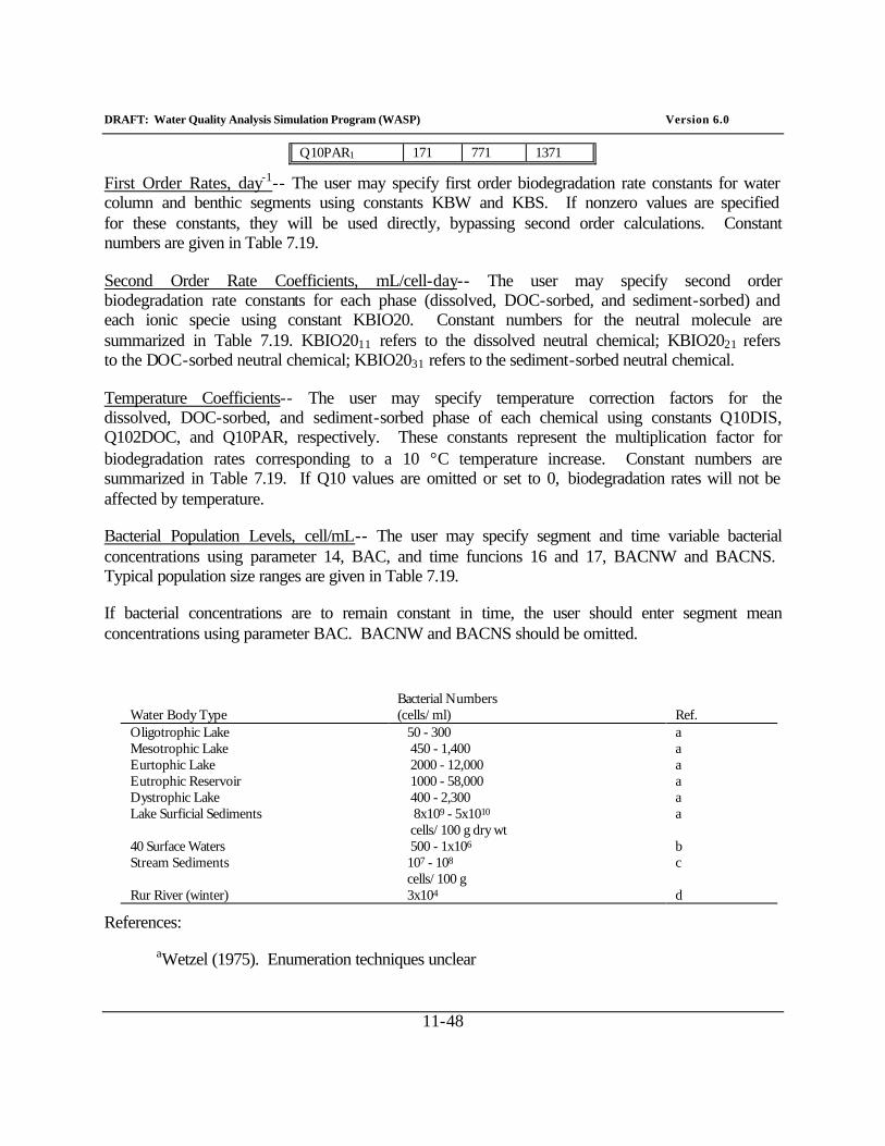
DRAFT: Water Quality Analysis Simulation Program (WASP) Version 6.0
11-48
Q10PAR1 171 771 1371
First Order Rates, day-1-- The user may specify first order biodegradation rate constants for water column and benthic segments using constants KBW and KBS. If nonzero values are specified for these constants, they will be used directly, bypassing second order calculations. Constant numbers are given in Table 7.19.
Second Order Rate Coefficients, mL/cell-day-- The user may specify second order biodegradation rate constants for each phase (dissolved, DOC-sorbed, and sediment-sorbed) and each ionic specie using constant KBIO20. Constant numbers for the neutral molecule are summarized in Table 7.19. KBIO2011 refers to the dissolved neutral chemical; KBIO2021 refers to the DOC-sorbed neutral chemical; KBIO2031 refers to the sediment-sorbed neutral chemical.
Temperature Coefficients-- The user may specify temperature correction factors for the dissolved, DOC-sorbed, and sediment-sorbed phase of each chemical using constants Q10DIS, Q102DOC, and Q10PAR, respectively. These constants represent the multiplication factor for biodegradation rates corresponding to a 10 °C temperature increase. Constant numbers are summarized in Table 7.19. If Q10 values are omitted or set to 0, biodegradation rates will not be affected by temperature.
Bacterial Population Levels, cell/mL-- The user may specify segment and time variable bacterial concentrations using parameter 14, BAC, and time funcions 16 and 17, BACNW and BACNS. Typical population size ranges are given in Table 7.19.
If bacterial concentrations are to remain constant in time, the user should enter segment mean concentrations using parameter BAC. BACNW and BACNS should be omitted.
Water Body Type
Bacterial Numbers (cells/ml)
Ref.
Oligotrophic Lake 50 - 300 a Mesotrophic Lake 450 - 1,400 a Eurtophic Lake 2000 - 12,000 a Eutrophic Reservoir 1000 - 58,000 a Dystrophic Lake 400 - 2,300 a Lake Surficial Sediments 8x10⁹ - 5x10¹⁰
cells/100 g dry wt a
40 Surface Waters 500 - 1x10⁶ b Stream Sediments 107 - 108
cells/100 g c
Rur River (winter) 3x10⁴ d
References:
aWetzel (1975). Enumeration techniques unclear

DRAFT: Water Quality Analysis Simulation Program (WASP) Version 6.0
11-49
bParis et al (1981). Bacterial enumeration using plate counts.
cHerbes & Schwall (1978). Bacterial enumeration using plate counts.
dLarson et al. (1981). Bacterial enumeration using plate counts.
The user may enter time-variable water column and benthic bacterial concentrations via time functions BACNW and BACNS, respectively, as a series of concentration versus time values. Parameter BAC will then represent the ratio of each segment concentration to the time function values. The product of BAC and the BACNW or BACNS function gives the segment and time specific bacterial concentrations used by TOXI. (Group G, Record 4, PARAM(I,14); Group I, Record 2, VALT(16,K), VALT(17,K))
11.11. Extra Reaction
An extra second-order reaction is included in TOXI. The second order reaction allows the user to simulate the effect of processes not considered by TOXI. The reaction depends upon a rate constant and a environmental parameter which may be taken to represent, for example, some reducing or oxidizing agent. The rate of reaction may also vary with temperature.
11.11.1. Overview of TOXI Extra Reaction
TOXI allows the user to specify an additional second order reaction for the various species and phases of each chemical:
Equation 11-73
f k [E] = K ij eij ji
E ∑∑
where:
KE = net extra reaction rate constant, day-1 [E] = intensity of environmental property driving this reaction keij = second order rate constant for chemical as specie in phase j,
in [E]-1 day-1 fij = fraction of chemical as specie i in phase j
The reaction coefficients may be specified as constants, with activation energy constants left as 0. If the user wants TOXI to determine rates based on the temperature based Arrhenius function, then non-zero activation energies specified, as constants will invoke the following calculation for each rate constant k:
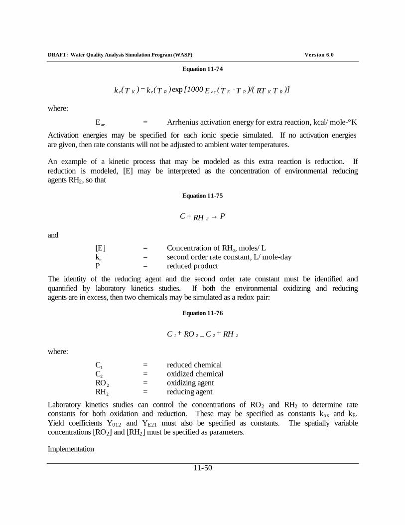
DRAFT: Water Quality Analysis Simulation Program (WASP) Version 6.0
11-50
Equation 11-74
)]T RT)/(T - T( E [1000 )T(k = )T(k R K R K ae R eK e exp
where:
Eae = Arrhenius activation energy for extra reaction, kcal/mole-°K
Activation energies may be specified for each ionic specie simulated. If no activation energies are given, then rate constants will not be adjusted to ambient water temperatures.
An example of a kinetic process that may be modeled as this extra reaction is reduction. If reduction is modeled, [E] may be interpreted as the concentration of environmental reducing agents RH2, so that
Equation 11-75
P RH + C 2 →
and
[E] = Concentration of RH2, moles/L ke = second order rate constant, L/mole-day P = reduced product
The identity of the reducing agent and the second order rate constant must be identified and quantified by laboratory kinetics studies. If both the environmental oxidizing and reducing agents are in excess, then two chemicals may be simulated as a redox pair:
Equation 11-76
RH + C RO + C 2 2 2 1 _
where:
C1 = reduced chemical C2 = oxidized chemical RO2 = oxidizing agent RH2 = reducing agent
Laboratory kinetics studies can control the concentrations of RO2 and RH2 to determine rate constants for both oxidation and reduction. These may be specified as constants kox and kE. Yield coefficients Y012 and YE21 must also be specified as constants. The spatially variable concentrations [RO2] and [RH2] must be specified as parameters.
Implementation
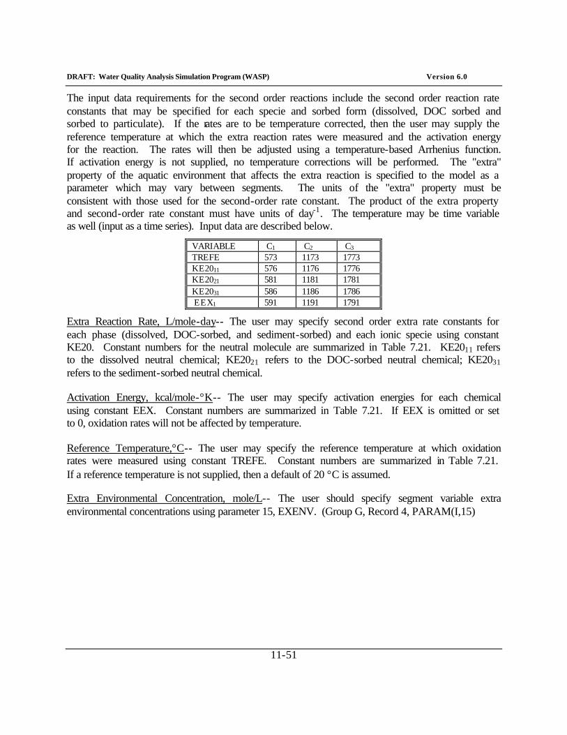
DRAFT: Water Quality Analysis Simulation Program (WASP) Version 6.0
11-51
The input data requirements for the second order reactions include the second order reaction rate constants that may be specified for each specie and sorbed form (dissolved, DOC sorbed and sorbed to particulate). If the rates are to be temperature corrected, then the user may supply the reference temperature at which the extra reaction rates were measured and the activation energy for the reaction. The rates will then be adjusted using a temperature-based Arrhenius function. If activation energy is not supplied, no temperature corrections will be performed. The "extra" property of the aquatic environment that affects the extra reaction is specified to the model as a parameter which may vary between segments. The units of the "extra" property must be consistent with those used for the second-order rate constant. The product of the extra property and second-order rate constant must have units of day-1. The temperature may be time variable as well (input as a time series). Input data are described below.
VARIABLE C1 C2 C3 TREFE 573 1173 1773 KE2011 576 1176 1776 KE2021 581 1181 1781 KE2031 586 1186 1786 EEX1 591 1191 1791
Extra Reaction Rate, L/mole-day-- The user may specify second order extra rate constants for each phase (dissolved, DOC-sorbed, and sediment-sorbed) and each ionic specie using constant KE20. Constant numbers for the neutral molecule are summarized in Table 7.21. KE2011 refers to the dissolved neutral chemical; KE2021 refers to the DOC-sorbed neutral chemical; KE2031 refers to the sediment-sorbed neutral chemical.
Activation Energy, kcal/mole-°K-- The user may specify activation energies for each chemical using constant EEX. Constant numbers are summarized in Table 7.21. If EEX is omitted or set to 0, oxidation rates will not be affected by temperature.
Reference Temperature,°C-- The user may specify the reference temperature at which oxidation rates were measured using constant TREFE. Constant numbers are summarized in Table 7.21. If a reference temperature is not supplied, then a default of 20 °C is assumed.
Extra Environmental Concentration, mole/L-- The user should specify segment variable extra environmental concentrations using parameter 15, EXENV. (Group G, Record 4, PARAM(I,15)
DRAFT: Water Quality Analysis Simulation Program (WASP) Version 6.0
12-1
12. REFERENCES
Alexander, M. 1980. Biodegradation of Toxic Chemicals in Water and Soil. In: Dynamics, Exposure, and Hazard Assessment of Toxic Chemicals, R. Haque, editor. Ann Arbor Science, Ann Arbor, MI.
Ambrose, R.B. 1987. Modeling Volatile Organics in the Delaware Estuary. American Society of Civil Engineers. Journal of Environmental Engineering, V. 113, No. 4, pp 703-721.
Ambrose, R.B. et al. 1988. WASP4, A Hydrodynamic and Water Quality Model--Model Theory, User's Manual, and Programmer's Guide. U.S. Environmental Protection Agency, Athens, GA. EPA/600/3-87-039.
APHA (American Public Health Association). 1985. Standard Methods for the Examination of Water and Wastewater, 15th Edition. APHA. Washington, DC.
Bannister, T.T. 1974a. Production Equations in Terms of Chlorophyll Concentration, Quantum Yield, and Upper Limit to Production. Limnol. Oceanogr. 19:1-12.
Bannister, T.T. 1974b. A General Theory of Steady State Phytoplankton Growth in a Nutrient Saturated Mixed Layer. Limnol. Oceanogr. 19:13-30.
Barber, M.C., L.A. Suarez, and R.R. Lassiter. 1991. Modelling Bioaccumulation of Organic Pollutants in Fish with an Application to PCBs in Lake Ontario Salmonids. Canadian J. Fisheries and Aquatic Sciences. Vol. 48, pp. 318-337.
Bella, D.A. and W.J. Grenney. 1970. Finite-Difference Convection Errors. Journal of the Sanitary Engineering Division, ASCE, Vol. 96, No. SA6, pp. 1361-1375.
Berner, R.A. 1974. Kinetic Models for the Early Digenesis of Nitrogen Sulfur, Phosphorus, and Silicon in Anoxic Marine Sediments. In: The Sea, Vol. 5, ed. E.D. Goldberg. J. Wiley and Sons. New York.
Bowie, G.L., W.B. Mills, D.B. Porcella, C.L. Campbell, J.R. Pagenkopf, G.L. Rupp, K.M. Johnson, P.W.H. Chan, S.A. Gherini and C.E. Chamberlin. 1985. Rates, Constants, and Kinetics Formulations in Surface Water Quality Modeling. Second Edition. U.S. Environmental Protection Agency Athens, GA. EPA-600/3-85-040.
Brown, L.C. and T.O. Barnwell. 1987. The Enhanced Stream Water Quality Models QUAL2E and QUAL2E-UNCAS: Documentation and User Manual. U.S. Environmental Protection Agency, Athens, GA. EPA/600/3-87-007.
Burns, L.A., D.M. Cline, and R.R. Lassiter. 1982. Exposure Analysis Modeling System (EXAMS): User Manual and System Documentation, U.S. Environmental Protection Agency, Athens, GA. EPA-600/3-82-023.
DRAFT: Water Quality Analysis Simulation Program (WASP) Version 6.0
12-2
Burns, L.A. and D.M. Cline. 1985. Exposure Analysis Modeling System, Reference Manual for EXAMS II. U.S. Environmental Protection Agency, Athens, GA. EPA-600/3-85-038.
Connolly, J.P. and R. Winfield. 1984. A User's Guide for WASTOX, a Framework for Modeling the Fate of Toxic Chemicals in Aquatic Environments. Part 1: Exposure Concentration. U.S. Environmental Protection Agency, Gulf Breeze, FL. EPA-600/3-84-077.
Connolly, J.P. and R.V. Thomann. 1985. WASTOX, A Framework for Modeling the Fate of Toxic Chemicals in Aquatic Environments. Part 2: Food Chain. U.S. Environmental Protection Agency, Gulf Breeze, FL and Duluth, MN. Covar, A.P. 1976. Selecting the Proper Reaeration Coefficient for Use in Water Quality Models. Presented at the U.S. EPA Conference on Env. Simulation and Modelling.
Covar, A.P. 1976. Selecting the Proper Reaeration Coefficient for Use in Water Quality Models. Presented at the U.S. EPA Conference on Environmental Simulation Modeling, April 19-22, 1976. Cincinnati, Ohio.
Di Toro, D.M., D.J. O'Connor, and R.V. Thomann. 1971. A Dynamic Model of the Phytoplankton Population in the Sacramento San Joaquin Delta. Adv. Chem. Ser. 106, Am. Chem. Soc., Washington, DC., pp. 131-180.
Di Toro, D.M. and J.P. Connolly. 1980. Mathematical Models of Water Quality in Large Lakes, Part 2: Lake Erie. EPA-600/3-80-065. pp. 90-101.
Di Toro, D.M. and W.F. Matystik. 1980. Mathematical Models of Water Quality in Large Lakes, Part 1: Lake Huron and Saginaw Bay. EPA-600/3-80-056. pp. 28-30.
Di Toro, D.M., J.J. Fitzpatrick, and R.V. Thomann. 1981, rev. 1983. Water Quality Analysis Simulation Program (WASP) and Model Verification Program (MVP) - Documentation. Hydroscience, Inc., Westwood, NY, for U.S. EPA, Duluth, MN, Contract No. 68-01-3872.
Di Toro, D.M. 1985. A Particle Interaction Model of Reversible Organic Chemical Sorption, Chemosphere 14(10):1503-1538.
Eppley, R.W. and P.R. Sloane. 1966. Growth Rates of Marine Phytoplankton: Correlation with Light Absorption by Cell Chlorophyll a. Physiol. Plant. 19:47-59.
Foree, E.C. and P.L. McCarty. 1970. Anaerobic Decomposition of Algae. Environ. Sci. & Technol. 4(10), pp. 842-849.
Graf, W.H. 1971. Hydraulics of Sediment Transport. McGraw-Hill, New York.
DRAFT: Water Quality Analysis Simulation Program (WASP) Version 6.0
12-3
Green, A.E.S., K.R. Cross, and L.A. Smith. 1980. Improved Analytical Characterization of Ultraviolet Skylight, Photochem. and Photobio. 31:59-65.
Hendry, G.S. 1977. Relationships Between Bacterial Levels and Other Characteristics of Recreational Lakes in the District of Muskoka. Interim Microbiology Report, Laboratory Services Branch, Ontario Ministry of the Environment.
Henrici, Arthur T., 1938. Seasonal Fluctuation of Lake Bacteria in Relation to Plankton Production. J. Bacteriol., 35:129-139.
Herbes, S.E. and L.R. Schwall. 1978. Microbial Transformation of Polycyclic Aromatic Hydrocarbons in Pristine and Petroleum-Contaminated Sediments. Appl. and Environ. Microbiology, Volume 35, No. 2. pp. 306-316.
Hutchinson, G.E. 1967. A Treatise on Limnology. Vol. II. Introduction to Lake Biology and Limnoplankton. Wiley. New York. pp. 306-354.
Jewell, W.J. And P.L. McCarty. 1971. Aerobic Decomposition of Algae. Environ. Sci. Technol. 1971. 5(10). p. 1023.
JRB, Inc. 1984. Development of Heavy Metal Waste Load Allocations for the Deep River, North Carolina. JRB Associates, McLean, VA, for U.S. EPA Office of Water Enforcement and Permits, Washington, DC.
Karickhoff, S.W., D.S. Brown, and T.A. Scott. 1979. Sorption of Hydrophobic Pollutants on Natural Sediments. Water Res. 13:241-248.
Karickhoff, S.W. 1984. Organic Pollutant Sorption in Aquatic Systems. J. Hydraul. Eng. Div. ASCE. Vol. 110, p. 707.
Karickhoff, S.W. and K.R. Morris. 1985. Sorption Dynamics of Hydrophobic Pollutants in Sediment Suspensions. Environ. Toxicology and Chem. 4:469-479.
Kok, B. 1960. Efficiency of Photosynthesis. In: W. Ruhland
(Edison), Hanbuch der Pfanzenphysiologie. Vol 5, Part 1. Springer, Berlin. pp. 563-633.
Larson, R.J. G.G. Clinckemaillie, and L. VanBelle. 1981. Effect of Temperature and Dissolved Oxygen on Biodegradation of Nitrilotriacetate. Water Research, Volume 15. pp. 615-620.
Leopold, L.B. and T. Maddox. 1953. The Hydraulic Geometry of Stream Channels and Some Physiographic Implications, Professional Paper 252, U.S. Geological Survey, Washington, DC.
Leopold, L.B., M.B. Wolman and J.P. Miller. 1964. Fluvial Processes in Geomorphology, W. H. Freeman and Co., San Francisco, CA.
DRAFT: Water Quality Analysis Simulation Program (WASP) Version 6.0
12-4
Lowe, W.E. 1976. Canada Centre for Inland Waters 867 Lakeshore Road, Burlington, Canada L7R 4A6. Personal communication.
Mackay, D. and P.J. Leinonen. 1975. Rate of Evaporation of Low-Solubility Contaminants from Water Bodies to Atmospheres. Environ. Sci. Technology. 7:611-614.
Mackay, D. and W.Y. Shiu. 1984. Physical-Chemical Phenomena and Molecular Properties, in Gas Transfer at Water Surfaces. Brutsaert, W. and G.H. Jirka, Eds. D. Reidel, Boston.
Menon, A.S., W.A. Gloschenko, and N.M. Burns. 1972. Bacteria-Phytoplankton Relationships in Lake Erie. Proc. 15th Conf. Great Lakes Res. 1972:94:101. Inter. Assoc. Great Lakes Res.
Mill, T., W.R. Mabey, P.C. Bomberger, T.W. Chou, D.G. Herdry, and J.H. Smith. 1982. Laboratory Protocols for Evaluating the Fate of Organic Chemicals in Air and Water. U.S. Environmental Protection Agency, Athens, GA. EPA-600/3-82-0220.
Mills, W.B., D.B. Porcella, M.J. Ungs, S.A. Gherini, K.V. Summers, Lingfung Mok, G.L. Rupp, G.L. Bowie, and D.A. Haith. 1985. Water Quality Assessment: A Screening Procedure for Toxic and Conventional Pollutants, Parts 1 and 2. U.S. Environmental Protection Agency, Athens, GA. EPA-600/6-85-002a and b.
Nriagu, J.O. 1972. Stability of Vivianite and Ion-Pair Formation in the System Fe3(PO4)2-H3PO4H20. Geochim. Cosmochim Acta. 36. p. 459.
O'Connor. D.J. and R.V. Thomann. 1972. Water Quality Models: Chemical, Physical and Biological Constituents. In: Estuarine Modeling: An Assessment. EPA Water Pollution Control Research Series 16070 DZV, Section 702/71. pp. 102-169.
O'Connor, D.J., J.A. Mueller, and K.J. Farley. 1983. Distribution of Kepone in the James River Estuary. Journal of the Environmental Engineering Division, ASCE. 109(EE2):396-413.
O'Connor, D.J. 1983. Wind Effects on Gas-Liquid Transfer Coefficients. Journal of Environmental Engineering, Volume 109, Number 9, pp. 731-752.
Paris, D.F., W.C. Steen, G.L. Baughman and J.T. Barnett, Jr. 1981. Second-Order Model to Predict Microbial Degradation of Organic Compounds in Natural Waters. Applied and Environmental Microbiology. 4(3):603-609.
Rao, S.S. 1976. Observations on Bacteriological Conditions in the Upper Great Lakes. 1968-1974. Scientific Series. No. 64. Inland Waters Directorate CCIW Branch, Burlington, Ontario.
DRAFT: Water Quality Analysis Simulation Program (WASP) Version 6.0
12-5
Rao, P.S.C. and J.M. Davidson. 1980. Estimation of Pesticide Retention and Transformation Parameters Required in Nonpoint Source Pollution Models. Environmental Impact of Nonpoint Source Pollution. Ann Arbor Science, Ann Arbor, MI. pp. 23-67.
Riley, G.A., H. Stommel and D.F. Bumpus. 1949. Quantitative Ecology of the Plankton of the Western North Atlantic. Bull. Bingham Oceanog. Coll. 12(3):1-169.
Robinson, N., ed. 1966. Solar Radiation. Elsevier Publishing, Amsterdam, London, and New York. 347 pp.
Smith, R.A. 1980. The Theoretical Basis for Estimating Phytoplankton Production and Specific Growth Rate from Chlorophyll, Light and Temperature Data. Ecological Modeling. 10. pp. 243-264.
Steele, J.H. 1962. Environmental Control of Photosynthesis in the Sea. Limnol. Oceanogr. 7:137-150.
Streeter, H.W. and E.B. Phelps. 1925. A Study of the Pollution and Natural Purification of the Ohio River, III, Factors Concerned in the Phenomena of Oxidation and Reaeration. U.S. Public Health Service, Public Health Bulletin No. 146, 75 pp. Reprinted by U.S. DHEW, PHA, 1958.
Thomann, R.V. 1975. Mathematical Modeling of Phytoplankton in Lake Ontario, 1. Model Development and Verification. U.S. Environmental Protection Agency, Corvallis, OR. EPA-600/3-75-005.
Thomann, R.V., R.P. Winfield, D.M. Di Toro, and D.J. O'Connor. 1976. Mathematical Modeling of Phytoplankton in Lake Ontario, 2. Simulations Using LAKE 1 Model. U.S. Environmental Protection Agency, Grosse Ile, MI, EPA-600/3-76-065.
Thomann, R.V., R.P. Winfield, and J.J. Segna. 1979. Verification Analysis of Lake Ontario and Rochester Embayment Three Dimensional Eutrophication Models. U.S. Environmental Protection Agency, Grosse Ile, MI, EPA-600/3-79-094.
Thomann, R.V. and J.J. Fitzpatrick. 1982. Calibration and Verification of a Mathematical Model of the Eutrophication of the Potomac Estuary. Prepared for Department of Environmental Services, Government of the District of Columbia, Washington, D.C.
Tsivoglou, E.E. and J.R. Wallace. 1972. Characterization of Stream Reaeration Capacity. U.S. Environmental Protection Agency, Washington, DC EPA-R3-72-012.
Warburg, O. and E. Negelein. 1923. Uber den einfluss der Wellenlange auf den Energieumsatz bei der Kohlensaureassimilation. A. Phys. Chem. 106:191-218.
DRAFT: Water Quality Analysis Simulation Program (WASP) Version 6.0
12-6
Weast, R.C., and M.J. Astle, ed. 1980. CRC Handbook of Chemistry and Physics. CRC Press, Boca Raton, FL.
Wetzel, R.G. 1975. Limnology. W.B. Saunders Co. Philadelphia. 743 pp.
Whitman, R.G. 1923. A Preliminary Experimental Confirmation of the Two-Film Theory of Gas Absorption. Chem. Metallurg. Eng. 29:146-148.
Wischmeier, W.H. and D.D. Smith. 1978. Predicting Rainfall Erosion Losses - A Guide to Conservation Planning. Agriculture Handbook No. 537. U.S. Dept. of Agriculture, Washington, DC.
Wolfe, N.L. 1980. Determining the Role of Hydrolysis in the Fate of Organics in Natural Waters. pp. 163-178 in R. Haque (Ed.) Dynamics, Exposure, and Hazard Assessment of Toxic Substances. Ann Arbor Science Publisheres, Ann Arbor.
Zepp, R.G. and D.M. Cline. 1977. Rates of Direct Photolysis in Aquatic Environment. Environ. Sci. Technol. 11:359-366.


![Apply with WASP Water Quality Model · WASP6 development is under Window of procedure[5].Developing in 2005 can under the Windows2000 and the XP system the WASP7 editionses of movement](https://img.pdfslide.us/doc/110x75/60be479cb7205709e47c0964/apply-with-wasp-water-quality-model-wasp6-development-is-under-window-of-procedure5developing.jpg)