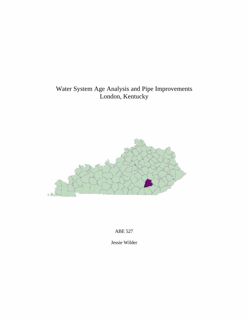
Water System Age Analysis and Pipe Improvements London, Kentucky

ABE 527

Jessie Wilder

1

Table of Contents

Section Page Abstract ...................................................................................................................................................2 Introduction

• Project Objectives and Significance ..............................................................................................2 • Background Information on London .............................................................................................3 • Literary Review..............................................................................................................................3

Methods • Modeling ........................................................................................................................................3 • Sensitivity.......................................................................................................................................4 • Calibration......................................................................................................................................5

Results and Discussion • Sensitivity Analysis .......................................................................................................................5 • Locating Problematic Pipes ...........................................................................................................6

Conclusion ..............................................................................................................................................8 Appendix A: Figures

2

Abstract: Within the old portion to downtown London, Kentucky, there is a system of very old pipes. The age of these pipes has caused the pipes to become rougher, causing flow problems in several areas of the system. This project created a model of the water system in this elder portion of town, performed a sensitivity analysis on this model, and found the pipes that contributed to the areas of low flow. The sensitivity analysis found the model to be sensitive to both pipe diameter and the roughness coefficient. However, the roughness coefficient was found to be the parameter with the highest sensitivity. The pipes within the system that contributed the greatest to the areas with low flow were pipes 7, 42, 44, and 52. By changing the roughness coefficients on these pipes until the flow at the problematic points in the model matched the flow a those point in the field, it was found that all four pipes need to be replaced in order for the flow at these problematic areas to increase. Introduction: Project Objectives and Significance: While performing a summer internship at Quest Engineers in Lexington, Kentucky, I was introduced to the City of London. During my first summer of work, Quest took on duties as town engineers for London. This means that Quest was put in charge of all water and wastewater system improvements and maintenances that the city requires. Over the past two years, Quest has begun work on some additions to London's current water system. In doing so, the city has asked that Quest also look at the old system and fix any problem areas that they come across. This is where my project comes into play. The objective of my project is to create a model, using the WaterCAD system, of the older portion of London's water system. Once the model is created, I aim to look at four problematic areas and determine the pipes within the system that contribute to the flow at those points. This would lead to the iteration of the most sensitive parameter of these contributing pipes, until the pressure at the nodes in question matches the pressure recorded in the field. The pipes in the worst condition will then be replaced with new pipes, and the model will be run again. Any effects that the new pipes have on the system will be recorded. Once the project has been successfully completed, my results will be presented to the water and wastewater department at Quest. While they are not relying on my data to complete improvements, they are interested to see if my conclusions match theirs, and to learn more about the capabilities of the WaterCAD modeling system.

3

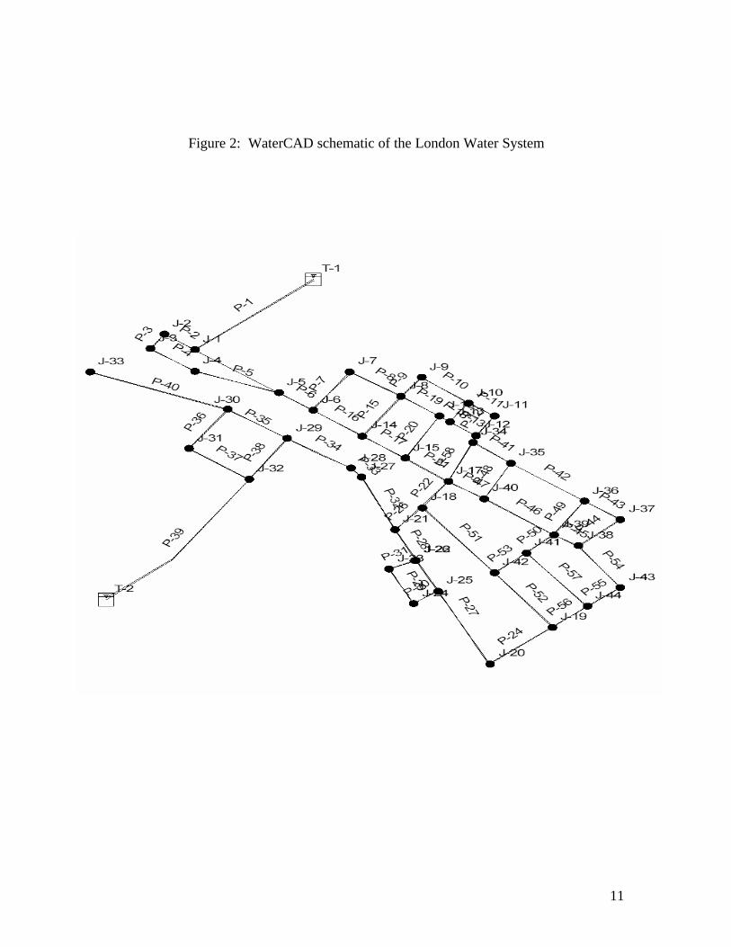
Background Information on London: The City of London is located in the southeast portion of Kentucky. London is the county seat of Laurel County, and according to the US Census Bureau, London has a population of 5,754 residents. Due to the extreme elevation changes that occur in London (elevation ranging from 700 to 1,700 feet above sea level), there are a total of 37 water towers within the city's system. While much of London's water system is relatively new, there is a small portion of the downtown area that dates well over 30 years old. This area is only fed by two water tanks, and is the area of interest for this report. A topographic map of the London area can be found in Appendix A, as Figure 1. Literature Review: Reference literature used to assist this project was exclusive to the Haestad Methods Water Modeling Manual. This reference was used when initially creating the WaterCAD model of the London system. It assisted in the acquisition of information for each node, pipe, and tank that allowed for the system to run properly. Methods: Modeling: The methods for modeling the London water system in WaterCAD were a multi-step process. The initial system layout was based off of system maps that were provided by the City of London and Quest Engineers. The maps provided were topographic maps of the city, with the pipes drawn in the correct locations. Exact lengths were not provided, so the lengths of the pipes drawn were converted by using the scale on the topographic maps. This was done with the assistance of the AutoCAD system. Topographic maps were loaded into AutoCAD, and the pipes were drawn in the correct locations in accordance with the maps provided by the City. AutoCAD was then able to calculate the lengths of portions of the piping system. The system was then re-drawn into WaterCAD, and the lengths of each pipe were entered into the pipe information tables. The WaterCAD system layout can be seen in Appendix A, Figure 2. The elevations at each junction node were found in the same manner as the pipe lengths. With the topographic map in the background, I was able to look at the pipe system drawn in AutoCAD and determine, to the best of my ability, the elevation at each node. These values were then entered into the WaterCAD system through the junction information tables. The elevation, size, and holding capacity of each tank were provided by the City of London. The flows at several nodes within the system were known and provided by Quest Engineers. The demands at other nodes were assumed based upon the number of houses connected to each particular node. A demand of 50 gal/day was assumed for each

4

household. This number came from assumed demands used in the Haestad Methods Textbook, in reference to a WaterCAD application. Sensitivity: Once the system model was running, a sensitivity analysis was performed on key parameters. A sensitivity analysis is run to determine which, if any parameters can be considered to be well determined, as apposed to poorly determined. Changes in a well-determined parameter will result in changes to the output of the model. In other words, the model will be sensitive to changes in that parameter. The two parameters that I chose to vary for my sensitivity analysis were the pipe diameter and the roughness coefficient. I chose these two parameters since my pipe system was old, and an old system is likely to have pipe diameters that have changed a bit due to build up or cavitation, as well as rougher pipes due to wear and tear. During the sensitivity analysis process, one node was chosen to monitor. Each pipe in the system was then selected, and the parameter that was being tested for was then changed. For instance, if the sensitivity was being run for the pipe diameter, each pipe diameter was changed and the system was run again. While changing the pipe diameter, the coefficient of roughness was held constant. Likewise, while changing the coefficient of roughness, the pipe diameter was held constant. After each run, the pressure at the chosen node was recorded. The system was run for the highest and lowest pipe diameters as well as the highest and lowest possible roughness coefficients. This amount of data was adequate for the calculation of sensitivity for each parameter. The sensitivity of each parameter is calculated from this information by using the following equation

S

b 2 b 1−

b 2 b 1+

2

p 2 p 1−

p 2 p 1+

2

:=

Where S is the relative sensitivity index, p1 is the lowest parameter, p2 is the highest parameter, b1 is the model result for the lowest parameter, and b2 is the model result for the highest parameter. Calibration: Unfortunately, I was unable to model the entire London water system due to a lack of available information. Thus, my model was only representative of the old portion of

5

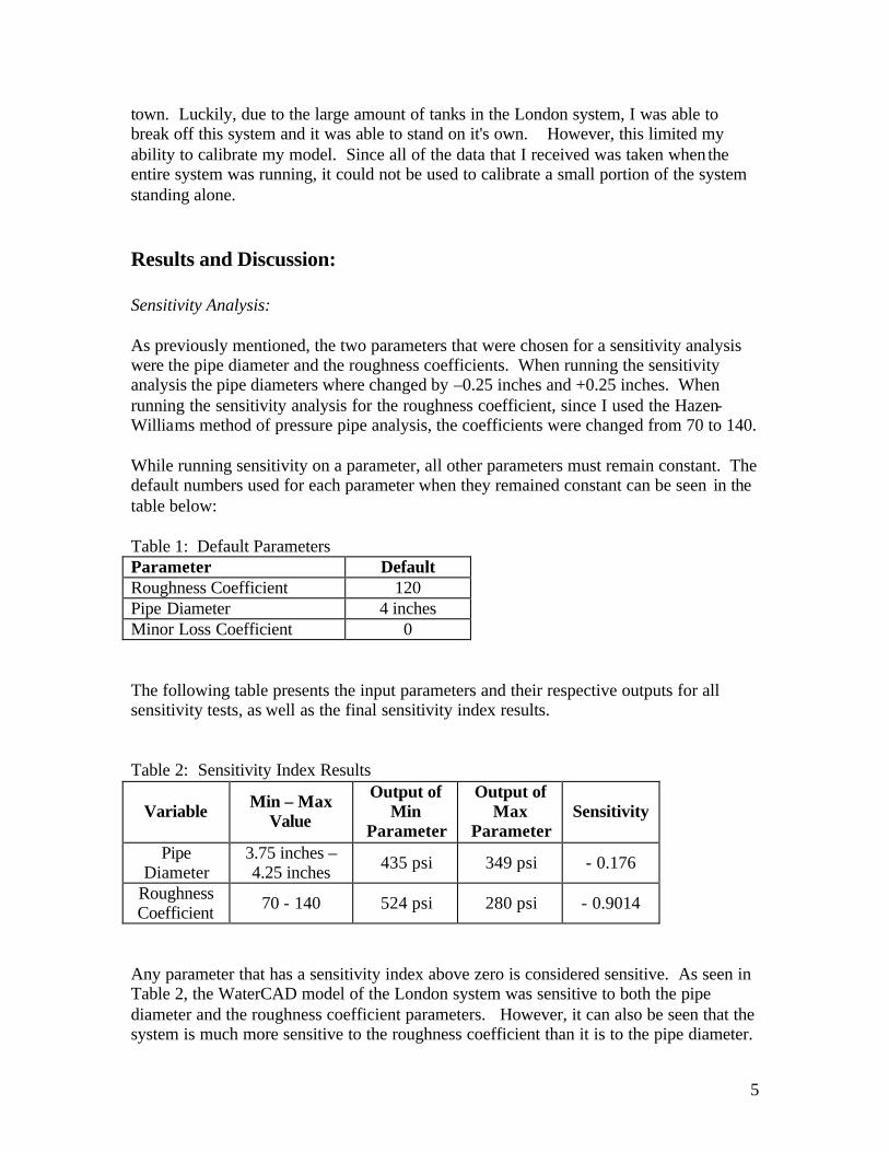
town. Luckily, due to the large amount of tanks in the London system, I was able to break off this system and it was able to stand on it's own. However, this limited my ability to calibrate my model. Since all of the data that I received was taken when the entire system was running, it could not be used to calibrate a small portion of the system standing alone. Results and Discussion: Sensitivity Analysis: As previously mentioned, the two parameters that were chosen for a sensitivity analysis were the pipe diameter and the roughness coefficients. When running the sensitivity analysis the pipe diameters where changed by –0.25 inches and +0.25 inches. When running the sensitivity analysis for the roughness coefficient, since I used the Hazen-Williams method of pressure pipe analysis, the coefficients were changed from 70 to 140. While running sensitivity on a parameter, all other parameters must remain constant. The default numbers used for each parameter when they remained constant can be seen in the table below: Table 1: Default Parameters Parameter Default Roughness Coefficient 120 Pipe Diameter 4 inches Minor Loss Coefficient 0

The following table presents the input parameters and their respective outputs for all sensitivity tests, as well as the final sensitivity index results. Table 2: Sensitivity Index Results

Variable Min – Max Value

Output of Min

Parameter

Output of Max

Parameter Sensitivity

Pipe Diameter

3.75 inches – 4.25 inches 435 psi 349 psi - 0.176

Roughness Coefficient 70 - 140 524 psi 280 psi - 0.9014

Any parameter that has a sensitivity index above zero is considered sensitive. As seen in Table 2, the WaterCAD model of the London system was sensitive to both the pipe diameter and the roughness coefficient parameters. However, it can also be seen that the system is much more sensitive to the roughness coefficient than it is to the pipe diameter.

6

This means that small changes in the roughness coefficient will have a much greater impact on the system then will small changes in the pipe diameter. Locating the Problematic Pipes: The process of locating the problematic pipes, proved to be quite tough. The problematic points of the system can be seen as the highlighted nodes in the WaterCAD figure below. Figure 1: Areas Receiving Low Flow

Each contributing pipe to each of these points was then labeled as a possible "problematic" pipe. Since the roughness coefficient was the most sensitive parameter, it would be the parameter that would need to be changed to simulate each old pipe. Since a lower roughness coefficient is representative of a rougher pipe, the coefficient was decreased slightly for each pipe to simulate the added roughness of old age, and then the system was run again. The figure below shows the pipes that were found to be the ones with the greatest impact on the problematic areas. These were pipes 7, 42, 44, and 52.

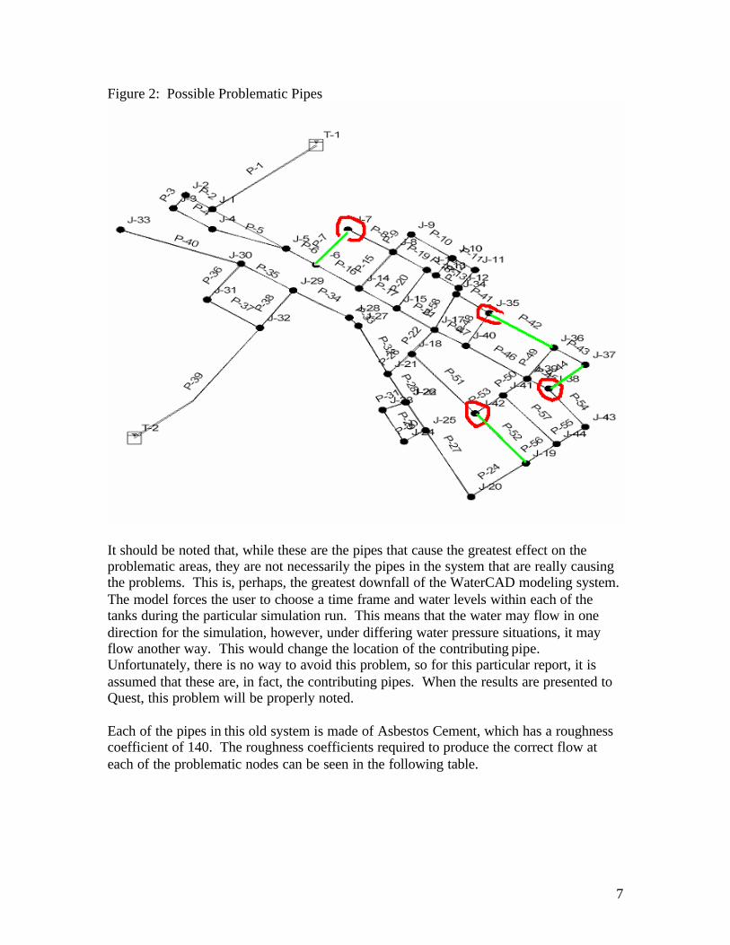
7

Figure 2: Possible Problematic Pipes

It should be noted that, while these are the pipes that cause the greatest effect on the problematic areas, they are not necessarily the pipes in the system that are really causing the problems. This is, perhaps, the greatest downfall of the WaterCAD modeling system. The model forces the user to choose a time frame and water levels within each of the tanks during the particular simulation run. This means that the water may flow in one direction for the simulation, however, under differing water pressure situations, it may flow another way. This would change the location of the contributing pipe. Unfortunately, there is no way to avoid this problem, so for this particular report, it is assumed that these are, in fact, the contributing pipes. When the results are presented to Quest, this problem will be properly noted. Each of the pipes in this old system is made of Asbestos Cement, which has a roughness coefficient of 140. The roughness coefficients required to produce the correct flow at each of the problematic nodes can be seen in the following table.

8

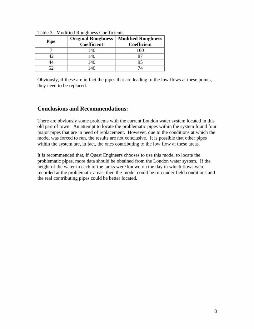
Table 3: Modified Roughness Coefficients

Pipe Original Roughness Coefficient

Modified Roughness Coefficient

7 140 100 42 140 87 44 140 95 52 140 74

Obviously, if these are in fact the pipes that are leading to the low flows at these points, they need to be replaced. Conclusions and Recommendations: There are obviously some problems with the current London water system located in this old part of town. An attempt to locate the problematic pipes within the system found four major pipes that are in need of replacement. However, due to the conditions at which the model was forced to run, the results are not conclusive. It is possible that other pipes within the system are, in fact, the ones contributing to the low flow at these areas. It is recommended that, if Quest Engineers chooses to use this model to locate the problematic pipes, more data should be obtained from the London water system. If the height of the water in each of the tanks were known on the day in which flows were recorded at the problematic areas, then the model could be run under field conditions and the real contributing pipes could be better located.

9

Appendix A

10

Figure 1: Topographic Map of the London Area

11

Figure 2: WaterCAD schematic of the London Water System