Chap 12-1 Statistics for Business and Economics, 6e © 2007 Pearson Education, Inc. Chapter 12 Simple Regression Statistics for Business and Economics 6

Chap 12-1Statistics for Business and Economics, 6e © 2007 Pearson Education, Inc.

Chapter 12

Simple Regression

Statistics for Business and Economics

6th Edition

Statistics for Business and Economics, 6e © 2007 Pearson Education, Inc. Chap 12-2

Chapter Goals

After completing this chapter, you should be able to:

Explain the correlation coefficient and perform a hypothesis test for zero population correlation

Explain the simple linear regression model Obtain and interpret the simple linear regression

equation for a set of data Describe R2 as a measure of explanatory power of the

regression model Understand the assumptions behind regression

analysis


Chapter Goals

After completing this chapter, you should be able to:

Explain measures of variation and determine whether the independent variable is significant

Calculate and interpret confidence intervals for the regression coefficients

Use a regression equation for prediction Form forecast intervals around an estimated Y value

for a given X Use graphical analysis to recognize potential problems

in regression analysis

(continued)


Correlation Analysis

Correlation analysis is used to measure strength of the association (linear relationship) between two variables Correlation is only concerned with strength of the

relationship

No causal effect is implied with correlation

Correlation was first presented in Chapter 3


Correlation Analysis

The population correlation coefficient is denoted ρ (the Greek letter rho)

The sample correlation coefficient is

yx

xy

ss

sr

1n

)y)(yx(xs ii

xy

where


To test the null hypothesis of no linear association,

the test statistic follows the Student’s t distribution with (n – 2 ) degrees of freedom:

Hypothesis Test for Correlation

0ρ:H0

)r(1

2)(nrt

2


Lower-tail test:

H0: ρ 0H1: ρ < 0

Upper-tail test:

H0: ρ ≤ 0H1: ρ > 0

Two-tail test:

H0: ρ = 0H1: ρ ≠ 0

Hypothesis Test for Correlation

Decision Rules

/2 /2

-t -t/2t t/2

Reject H0 if t < -tn-2, Reject H0 if t > tn-2, Reject H0 if t < -tn-2,

or t > tn-2,

Where has n - 2 d.f.)r(1

2)(nrt

2


Introduction to Regression Analysis

Regression analysis is used to: Predict the value of a dependent variable based on

the value of at least one independent variable

Explain the impact of changes in an independent variable on the dependent variable

Dependent variable: the variable we wish to explain (also called the endogenous variable)

Independent variable: the variable used to explain the dependent variable (also called the exogenous variable)


Linear Regression Model

The relationship between X and Y is described by a linear function

Changes in Y are assumed to be caused by changes in X

Linear regression population equation model

Where 0 and 1 are the population model coefficients and is a random error term.

ii10i εxββY


ii10i εXββY Linear component

Simple Linear Regression Model

The population regression model:

Population Y intercept

Population SlopeCoefficient

Random Error term

Dependent Variable

Independent Variable

Random Error component


(continued)

Random Error for this Xi value

Y

X

Observed Value of Y for Xi

Predicted Value of Y for Xi

ii10i εXββY

Xi

Slope = β1

Intercept = β0

εi

Simple Linear Regression Model


i10i xbby ˆ

The simple linear regression equation provides an estimate of the population regression line

Simple Linear Regression Equation

Estimate of the regression

intercept

Estimate of the regression slope

Estimated (or predicted) y value for observation i

Value of x for observation i

The individual random error terms ei have a mean of zero

))ˆ( i10iiii xb(b-yy-ye


Least Squares Estimators

b0 and b1 are obtained by finding the values

of b0 and b1 that minimize the sum of the

squared differences between y and :

2i10i

2ii

2i

)]xb(b[y min

)y(y min

e minSSE min

ˆ

y

Differential calculus is used to obtain the coefficient estimators b0 and b1 that minimize SSE


The slope coefficient estimator is

And the constant or y-intercept is

The regression line always goes through the mean x, y

X

Yxyn

1i

2i

n

1iii

1 s

sr

)x(x

)y)(yx(xb

xbyb 10

xx

Least Squares Estimators(continued)


Finding the Least Squares Equation

The coefficients b0 and b1 , and other regression results in this chapter, will be found using a computer Hand calculations are tedious

Statistical routines are built into Excel

Other statistical analysis software can be used


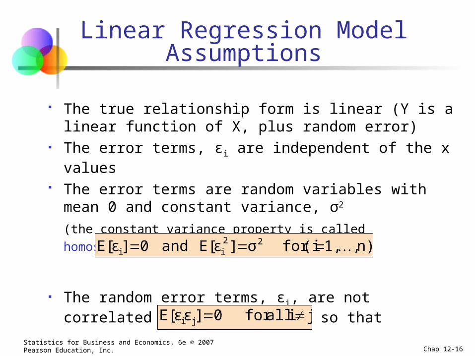
Linear Regression Model Assumptions

The true relationship form is linear (Y is a linear function of X, plus random error)

The error terms, εi are independent of the x values The error terms are random variables with mean 0 and

constant variance, σ2

(the constant variance property is called homoscedasticity)

The random error terms, εi, are not correlated with one another, so that

n), 1,(i for σ]E[εand0]E[ε 22ii

ji all for 0]εE[ε ji


b0 is the estimated average value of y

when the value of x is zero (if x = 0 is in the range of observed x values)

b1 is the estimated change in the

average value of y as a result of a one-unit change in x

Interpretation of the Slope and the Intercept


Simple Linear Regression Example

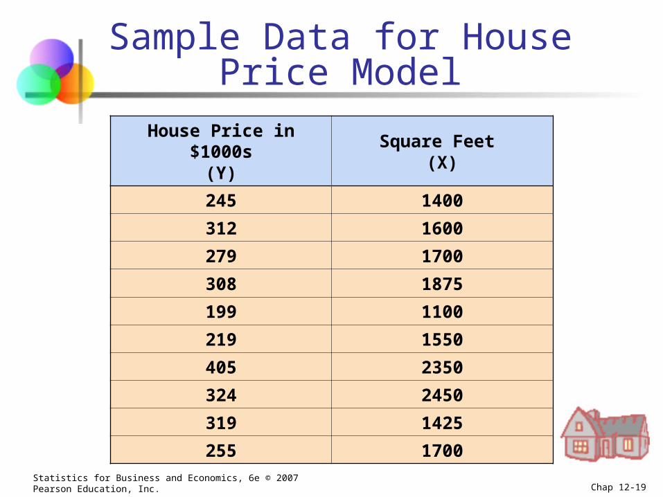
A real estate agent wishes to examine the relationship between the selling price of a home and its size (measured in square feet)

A random sample of 10 houses is selected Dependent variable (Y) = house price in $1000s Independent variable (X) = square feet


Sample Data for House Price Model

House Price in $1000s(Y)

Square Feet (X)

245 1400

312 1600

279 1700

308 1875

199 1100

219 1550

405 2350

324 2450

319 1425

255 1700


0

50

100

150

200

250

300

350

400

450

0 500 1000 1500 2000 2500 3000

Square Feet

Ho

use

Pri

ce (

$100

0s)

Graphical Presentation

House price model: scatter plot


Regression Using Excel

Tools / Data Analysis / Regression


Excel Output

Regression Statistics

Multiple R 0.76211

R Square 0.58082

Adjusted R Square 0.52842

Standard Error 41.33032

Observations 10

ANOVA df SS MS F Significance F

Regression 1 18934.9348 18934.9348 11.0848 0.01039

Residual 8 13665.5652 1708.1957

Total 9 32600.5000

Coefficients Standard Error t Stat P-value Lower 95% Upper 95%

Intercept 98.24833 58.03348 1.69296 0.12892 -35.57720 232.07386

Square Feet 0.10977 0.03297 3.32938 0.01039 0.03374 0.18580

The regression equation is:

feet) (square 0.10977 98.24833 price house


0

50

100

150

200

250

300

350

400

450

0 500 1000 1500 2000 2500 3000

Square Feet

Ho

use

Pri

ce (

$100

0s)

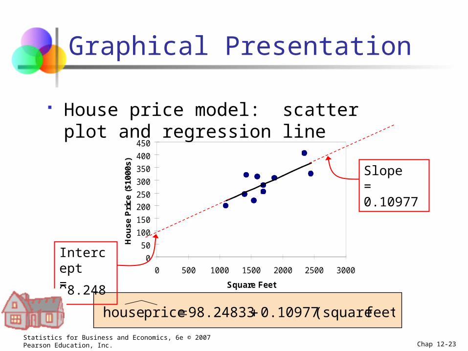
Graphical Presentation

House price model: scatter plot and regression line


Slope = 0.10977

Intercept = 98.248


Interpretation of the Intercept, b0

b0 is the estimated average value of Y when the

value of X is zero (if X = 0 is in the range of observed X values)

Here, no houses had 0 square feet, so b0 = 98.24833

just indicates that, for houses within the range of sizes observed, $98,248.33 is the portion of the house price not explained by square feet



Interpretation of the Slope Coefficient, b1

b1 measures the estimated change in the

average value of Y as a result of a one-unit change in X Here, b1 = .10977 tells us that the average value of a

house increases by .10977($1000) = $109.77, on average, for each additional one square foot of size



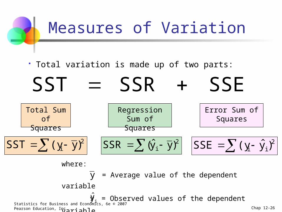
Measures of Variation

Total variation is made up of two parts:

SSE SSR SST Total Sum of

SquaresRegression Sum

of SquaresError Sum of

Squares

2i )y(ySST 2

ii )y(ySSE ˆ 2i )yy(SSR ˆ

where:

= Average value of the dependent variable

yi = Observed values of the dependent variable

i = Predicted value of y for the given xi valuey

y


SST = total sum of squares

Measures the variation of the yi values around their mean, y

SSR = regression sum of squares

Explained variation attributable to the linear relationship between x and y

SSE = error sum of squares

Variation attributable to factors other than the linear relationship between x and y

(continued)



(continued)

xi

y

X

yi

SST = (yi - y)2

SSE = (yi - yi )2

SSR = (yi - y)2

_

_

_

y

Y

y_y



The coefficient of determination is the portion of the total variation in the dependent variable that is explained by variation in the independent variable

The coefficient of determination is also called R-squared and is denoted as R2

Coefficient of Determination, R2

1R0 2 note:

squares of sum total

squares of sum regression

SST

SSRR2


r2 = 1

Examples of Approximate r2 Values

Y

X

Y

X

r2 = 1

r2 = 1

Perfect linear relationship between X and Y:

100% of the variation in Y is explained by variation in X



Y

X

Y

X

0 < r2 < 1

Weaker linear relationships between X and Y:

Some but not all of the variation in Y is explained by variation in X



r2 = 0

No linear relationship between X and Y:

The value of Y does not depend on X. (None of the variation in Y is explained by variation in X)

Y

Xr2 = 0


Excel Output


Multiple R 0.76211

R Square 0.58082



Observations 10


Regression 1 18934.9348 18934.9348 11.0848 0.01039

Residual 8 13665.5652 1708.1957

Total 9 32600.5000


Intercept 98.24833 58.03348 1.69296 0.12892 -35.57720 232.07386

Square Feet 0.10977 0.03297 3.32938 0.01039 0.03374 0.18580

58.08% of the variation in house prices is explained by

variation in square feet

0.5808232600.5000

18934.9348

SST

SSRR2


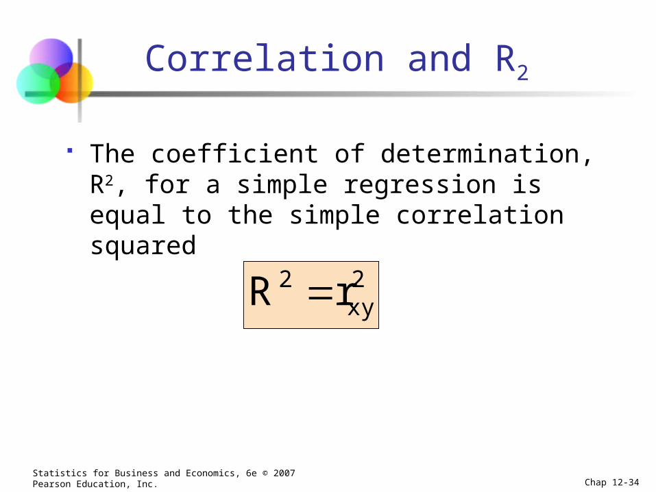
Correlation and R2

The coefficient of determination, R2, for a simple regression is equal to the simple correlation squared

2xy

2 rR


Estimation of Model Error Variance

An estimator for the variance of the population model error is

Division by n – 2 instead of n – 1 is because the simple regression model uses two estimated parameters, b0 and b1, instead of one

is called the standard error of the estimate

2n

SSE

2n

esσ

n

1i

2i

2e

2

ˆ

2ee ss


Excel Output


Multiple R 0.76211

R Square 0.58082



Observations 10


Regression 1 18934.9348 18934.9348 11.0848 0.01039

Residual 8 13665.5652 1708.1957

Total 9 32600.5000


Intercept 98.24833 58.03348 1.69296 0.12892 -35.57720 232.07386

Square Feet 0.10977 0.03297 3.32938 0.01039 0.03374 0.18580

41.33032se


Comparing Standard Errors

YY

X Xes small es large

se is a measure of the variation of observed y values from the regression line

The magnitude of se should always be judged relative to the size of the y values in the sample data

i.e., se = $41.33K is moderately small relative to house prices in

the $200 - $300K range


Inferences About the Regression Model

The variance of the regression slope coefficient (b1) is estimated by

2x

2e

2i

2e2

1)s(n

s

)x(x

ss

1b

where:

= Estimate of the standard error of the least squares slope

= Standard error of the estimate

1bs

2n

SSEse


Excel Output


Multiple R 0.76211

R Square 0.58082



Observations 10


Regression 1 18934.9348 18934.9348 11.0848 0.01039

Residual 8 13665.5652 1708.1957

Total 9 32600.5000


Intercept 98.24833 58.03348 1.69296 0.12892 -35.57720 232.07386

Square Feet 0.10977 0.03297 3.32938 0.01039 0.03374 0.18580

0.03297s1b


Comparing Standard Errors of the Slope

Y

X

Y

X1bS small

1bS large

is a measure of the variation in the slope of regression lines from different possible samples

1bS


Inference about the Slope: t Test

t test for a population slope Is there a linear relationship between X and Y?

Null and alternative hypotheses H0: β1 = 0 (no linear relationship)

H1: β1 0 (linear relationship does exist)

Test statistic

1b

11

s

βbt

2nd.f.

where:

b1 = regression slope coefficient

β1 = hypothesized slope

sb1 = standard error of the slope


House Price in $1000s

(y)

Square Feet (x)

245 1400

312 1600

279 1700

308 1875

199 1100

219 1550

405 2350

324 2450

319 1425

255 1700

(sq.ft.) 0.1098 98.25 price house

Estimated Regression Equation:

The slope of this model is 0.1098

Does square footage of the house affect its sales price?

Inference about the Slope: t Test

(continued)


Inferences about the Slope: t Test Example

H0: β1 = 0

H1: β1 0

From Excel output: Coefficients Standard Error t Stat P-value

Intercept 98.24833 58.03348 1.69296 0.12892

Square Feet 0.10977 0.03297 3.32938 0.01039

1bs

t

b1

3.329380.03297

00.10977

s

βbt

1b

11



H0: β1 = 0

H1: β1 0

Test Statistic: t = 3.329

There is sufficient evidence that square footage affects house price

From Excel output:

Reject H0

Coefficients Standard Error t Stat P-value

Intercept 98.24833 58.03348 1.69296 0.12892

Square Feet 0.10977 0.03297 3.32938 0.01039

1bs tb1

Decision:

Conclusion:

Reject H0Reject H0

/2=.025

-tn-2,α/2

Do not reject H0

0

/2=.025

-2.3060 2.3060 3.329

d.f. = 10-2 = 8

t8,.025 = 2.3060

(continued)

tn-2,α/2



H0: β1 = 0

H1: β1 0

P-value = 0.01039

There is sufficient evidence that square footage affects house price

From Excel output:

Reject H0

Coefficients Standard Error t Stat P-value

Intercept 98.24833 58.03348 1.69296 0.12892

Square Feet 0.10977 0.03297 3.32938 0.01039

P-value

Decision: P-value < α so

Conclusion:

(continued)

This is a two-tail test, so the p-value is

P(t > 3.329)+P(t < -3.329) = 0.01039

(for 8 d.f.)


Confidence Interval Estimate for the Slope

Confidence Interval Estimate of the Slope:

Excel Printout for House Prices:

At 95% level of confidence, the confidence interval for the slope is (0.0337, 0.1858)

11 bα/22,n11bα/22,n1 stbβstb


Intercept 98.24833 58.03348 1.69296 0.12892 -35.57720 232.07386

Square Feet 0.10977 0.03297 3.32938 0.01039 0.03374 0.18580

d.f. = n - 2


Since the units of the house price variable is $1000s, we are 95% confident that the average impact on sales price is between $33.70 and $185.80 per square foot of house size


Intercept 98.24833 58.03348 1.69296 0.12892 -35.57720 232.07386

Square Feet 0.10977 0.03297 3.32938 0.01039 0.03374 0.18580

This 95% confidence interval does not include 0.

Conclusion: There is a significant relationship between house price and square feet at the .05 level of significance

Confidence Interval Estimate for the Slope

(continued)


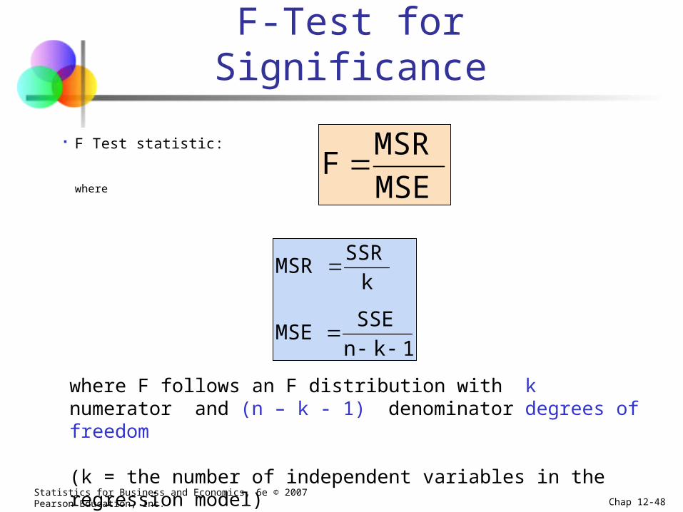
F-Test for Significance

F Test statistic:

where

MSE

MSRF

1kn

SSEMSE

k

SSRMSR

where F follows an F distribution with k numerator and (n – k - 1) denominator degrees of freedom

(k = the number of independent variables in the regression model)


Excel Output


Multiple R 0.76211

R Square 0.58082



Observations 10


Regression 1 18934.9348 18934.9348 11.0848 0.01039

Residual 8 13665.5652 1708.1957

Total 9 32600.5000


Intercept 98.24833 58.03348 1.69296 0.12892 -35.57720 232.07386

Square Feet 0.10977 0.03297 3.32938 0.01039 0.03374 0.18580

11.08481708.1957

18934.9348

MSE

MSRF

With 1 and 8 degrees of freedom

P-value for the F-Test


H0: β1 = 0

H1: β1 ≠ 0

= .05

df1= 1 df2 = 8

Test Statistic:

Decision:

Conclusion:

Reject H0 at = 0.05

There is sufficient evidence that house size affects selling price0

= .05

F.05 = 5.32Reject H0Do not

reject H0

11.08MSE

MSRF

Critical Value:

F = 5.32

F-Test for Significance(continued)

F


Prediction

The regression equation can be used to predict a value for y, given a particular x

For a specified value, xn+1 , the predicted value is

1n101n xbby ˆ


317.85

0)0.1098(200 98.25

(sq.ft.) 0.1098 98.25 price house

Predict the price for a house with 2000 square feet:

The predicted price for a house with 2000 square feet is 317.85($1,000s) = $317,850

Predictions Using Regression Analysis


0

50

100

150

200

250

300

350

400

450

0 500 1000 1500 2000 2500 3000

Square Feet

Ho

use

Pri

ce (

$100

0s)

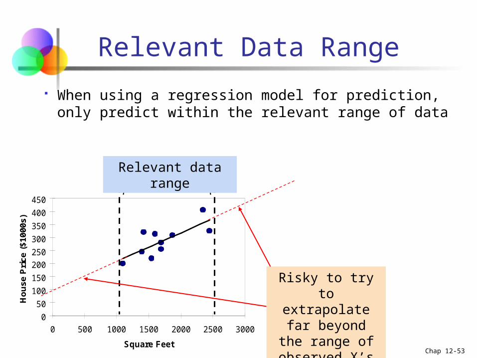
Relevant Data Range

When using a regression model for prediction, only predict within the relevant range of data

Relevant data range

Risky to try to extrapolate far

beyond the range of observed X’s


Estimating Mean Values and Predicting Individual Values

Y

X xi

y = b0+b1xi

Confidence Interval for the expected value of y,

given xi

Prediction Interval for an single

observed y, given xi

Goal: Form intervals around y to express uncertainty about the value of y for a given xi

y


Confidence Interval for the Average Y, Given X

Confidence interval estimate for the expected value of y given a particular xi

Notice that the formula involves the term

so the size of interval varies according to the distance

xn+1 is from the mean, x

2i

21n

eα/22,n1n

1n1n

)x(x

)x(x

n

1sty

:)X|E(Y for interval Confidence

ˆ

21n )x(x


Prediction Interval for an Individual Y, Given X

Confidence interval estimate for an actual observed value of y given a particular xi

This extra term adds to the interval width to reflect the added uncertainty for an individual case

2i

21n

eα/22,n1n

1n

)x(x

)x(x

n

11sty

:y for interval Confidence

ˆ

ˆ


Estimation of Mean Values: Example

Find the 95% confidence interval for the mean price of 2,000 square-foot houses

Predicted Price yi = 317.85 ($1,000s)

Confidence Interval Estimate for E(Yn+1|Xn+1)

37.12317.85)x(x

)x(x

n

1sty

2i

2i

eα/22,-n1n

ˆ

The confidence interval endpoints are 280.66 and 354.90, or from $280,660 to $354,900


Estimation of Individual Values: Example

Find the 95% confidence interval for an individual house with 2,000 square feet

Predicted Price yi = 317.85 ($1,000s)

Confidence Interval Estimate for yn+1

102.28317.85)X(X

)X(X

n

11sty

2i

2i

eα/21,-n1n

ˆ

The confidence interval endpoints are 215.50 and 420.07, or from $215,500 to $420,070


Finding Confidence and Prediction Intervals in Excel

In Excel, use

PHStat | regression | simple linear regression …

Check the

“confidence and prediction interval for x=”

box and enter the x-value and confidence level desired


Input values

Finding Confidence and Prediction Intervals in Excel

(continued)

Confidence Interval Estimate for E(Yn+1|Xn+1)

Confidence Interval Estimate for individual yn+1

y


Graphical Analysis

The linear regression model is based on minimizing the sum of squared errors

If outliers exist, their potentially large squared errors may have a strong influence on the fitted regression line

Be sure to examine your data graphically for outliers and extreme points

Decide, based on your model and logic, whether the extreme points should remain or be removed


Chapter Summary

Introduced the linear regression model Reviewed correlation and the assumptions of

linear regression Discussed estimating the simple linear

regression coefficients Described measures of variation Described inference about the slope Addressed estimation of mean values and

prediction of individual values

Documents

Chap 12-1 Statistics for Business and Economics, 6e © 2007 Pearson Education, Inc. Chapter 12 Simple Regression Statistics for Business and Economics 6