Embed Size (px)
Citation preview
Chap 15-1Statistics for Business and Economics, 6e © 2007 Pearson Education, Inc.
Chapter 15
Nonparametric Statistics
Statistics for Business and Economics
6th Edition
Statistics for Business and Economics, 6e © 2007 Pearson Education, Inc. Chap 15-2
Chapter Goals
After completing this chapter, you should be able to: Use the sign test for paired or matched samples Use a sign test for a single population median Recognize when and how to use the Wilcoxon signed
rank test for a population median Apply a normal approximation for the Wilcoxon signed
rank test Know when and how to perform a Mann-Whitney U-test Explain Spearman rank correlation and perform a test
for association
Statistics for Business and Economics, 6e © 2007 Pearson Education, Inc. Chap 15-3
Nonparametric Statistics
Nonparametric Statistics Fewer restrictive assumptions about data
levels and underlying probability distributions Population distributions may be skewed The level of data measurement may only be
ordinal or nominal
Statistics for Business and Economics, 6e © 2007 Pearson Education, Inc. Chap 15-4
Sign Test and Confidence Interval
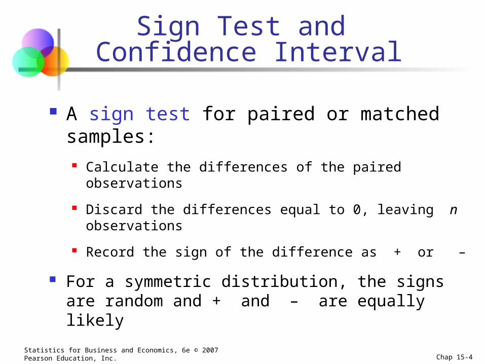
A sign test for paired or matched samples: Calculate the differences of the paired observations
Discard the differences equal to 0, leaving n observations
Record the sign of the difference as + or –
For a symmetric distribution, the signs are random and + and – are equally likely
Statistics for Business and Economics, 6e © 2007 Pearson Education, Inc. Chap 15-5
Sign Test
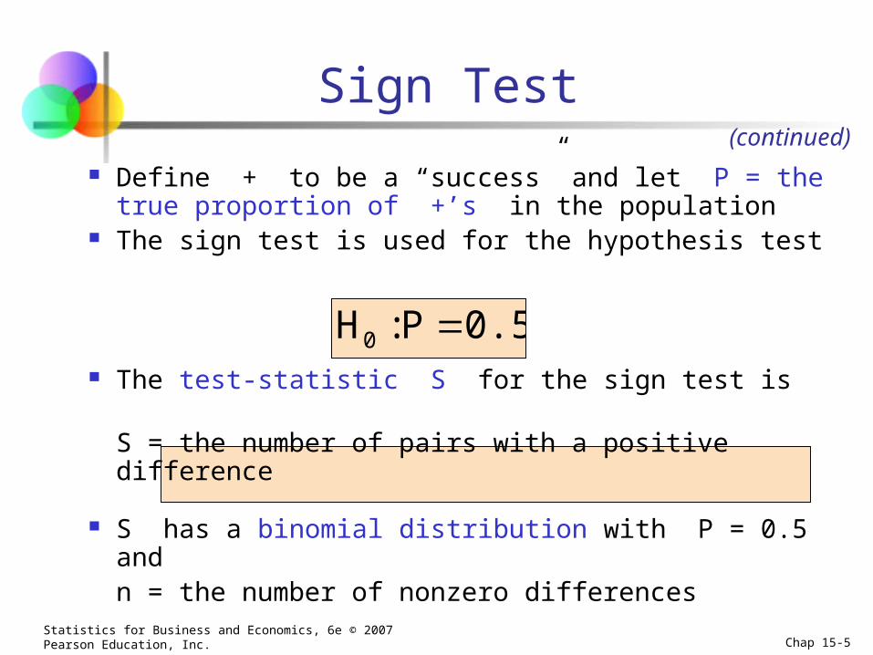
Define + to be a “success” and let P = the true proportion of +’s in the population
The sign test is used for the hypothesis test
The test-statistic S for the sign test is
S = the number of pairs with a positive difference
S has a binomial distribution with P = 0.5 and n = the number of nonzero differences
(continued)
0.5P:H0
Statistics for Business and Economics, 6e © 2007 Pearson Education, Inc. Chap 15-6
Determining the p-value
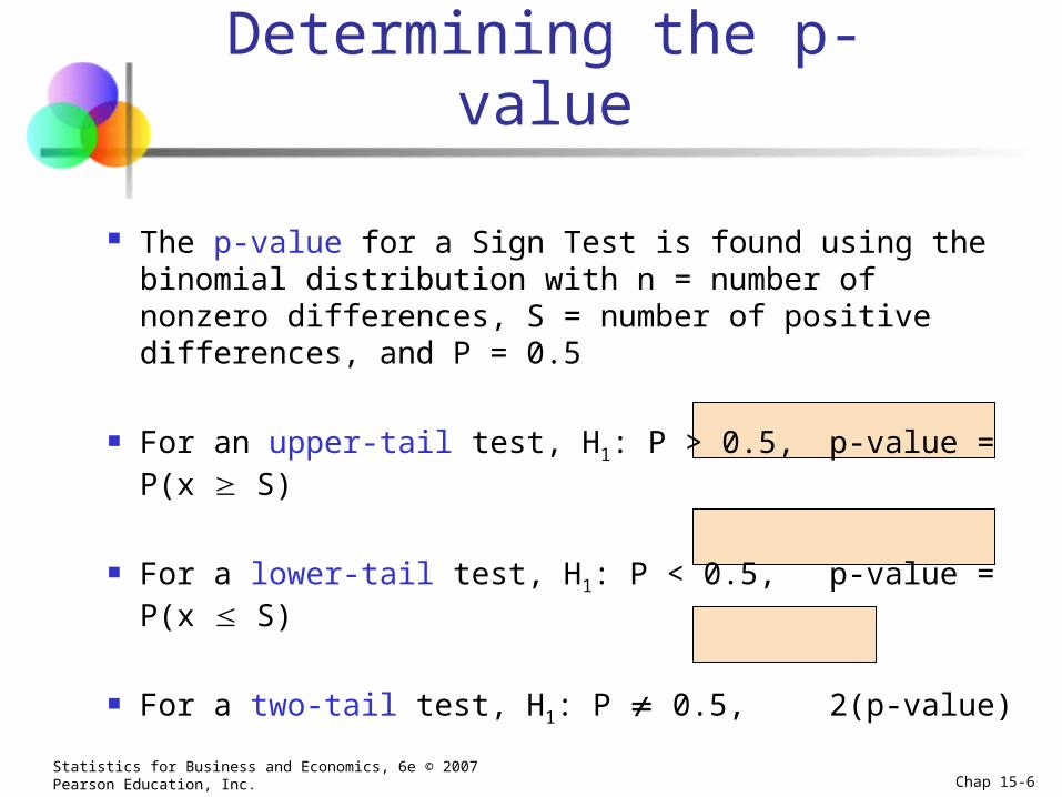
The p-value for a Sign Test is found using the binomial distribution with n = number of nonzero differences, S = number of positive differences, and P = 0.5
For an upper-tail test, H1: P > 0.5, p-value = P(x S)
For a lower-tail test, H1: P < 0.5, p-value = P(x S)
For a two-tail test, H1: P 0.5, 2(p-value)
Statistics for Business and Economics, 6e © 2007 Pearson Education, Inc. Chap 15-7
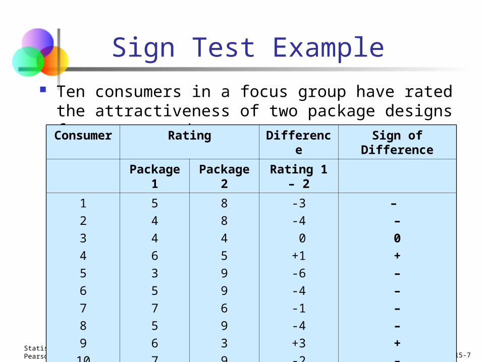
Sign Test Example Ten consumers in a focus group have rated the
attractiveness of two package designs for a new product
Consumer Rating Difference Sign of Difference
Package 1 Package 2 Rating 1 – 2
1
2
3
4
5
6
7
8
9
10
5
4
4
6
3
5
7
5
6
7
8
8
4
5
9
9
6
9
3
9
-3
-4
0
+1
-6
-4
-1
-4
+3
-2
–
–
0
+
–
–
–
–
+
–
Statistics for Business and Economics, 6e © 2007 Pearson Education, Inc. Chap 15-8
Sign Test Example(continued)
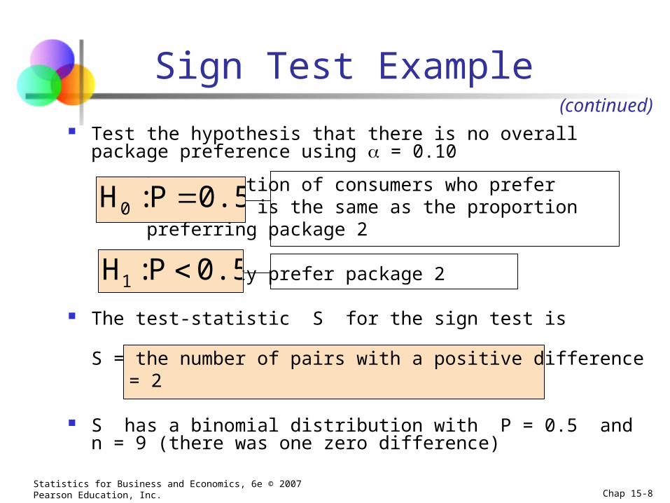
Test the hypothesis that there is no overall package preference using = 0.10
The proportion of consumers who prefer package 1 is the same as the proportion preferring package 2
A majority prefer package 2
The test-statistic S for the sign test is
S = the number of pairs with a positive difference = 2
S has a binomial distribution with P = 0.5 and n = 9 (there was one zero difference)
0.5P:H0
0.5P:H1
Statistics for Business and Economics, 6e © 2007 Pearson Education, Inc. Chap 15-9
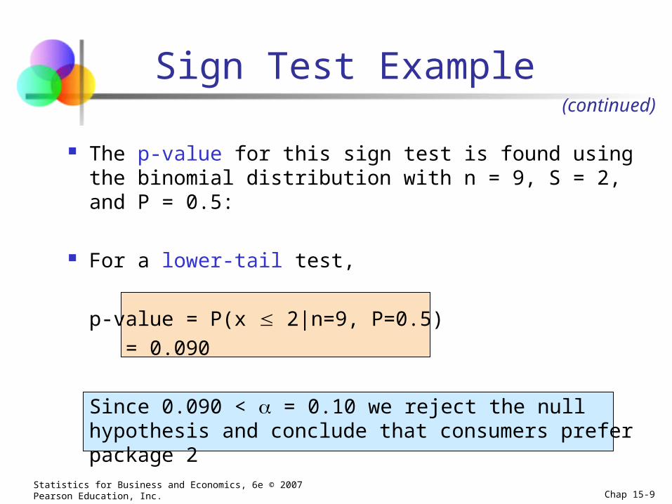
The p-value for this sign test is found using the binomial distribution with n = 9, S = 2, and P = 0.5:
For a lower-tail test,
p-value = P(x 2|n=9, P=0.5)
= 0.090
Since 0.090 < = 0.10 we reject the null hypothesis and conclude that consumers prefer package 2
Sign Test Example(continued)
Statistics for Business and Economics, 6e © 2007 Pearson Education, Inc. Chap 15-10
Sign Test: Normal Approximation
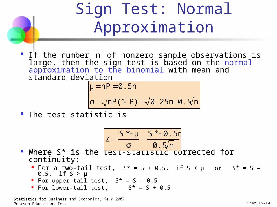
If the number n of nonzero sample observations is large, then the sign test is based on the normal approximation to the binomial with mean and standard deviation
The test statistic is
Where S* is the test-statistic corrected for continuity: For a two-tail test, S* = S + 0.5, if S < μ or S* = S – 0.5, if S > μ For upper-tail test, S* = S – 0.5 For lower-tail test, S* = S + 0.5
n0.50.25nP)nP(1σ
0.5nnPμ
n0.5
0.5n*S
σ
μ*SZ
Statistics for Business and Economics, 6e © 2007 Pearson Education, Inc. Chap 15-11
Sign Test for Single Population Median
The sign test can be used to test that a single population median is equal to a specified value
For small samples, use the binomial distribution
For large samples, use the normal approximation
Statistics for Business and Economics, 6e © 2007 Pearson Education, Inc. Chap 15-12
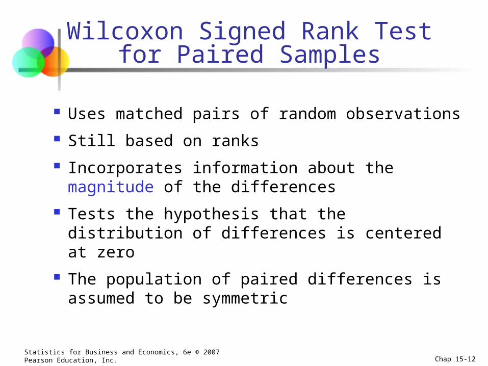
Wilcoxon Signed Rank Test for Paired Samples
Uses matched pairs of random observations
Still based on ranks
Incorporates information about the magnitude of the differences
Tests the hypothesis that the distribution of differences is centered at zero
The population of paired differences is assumed to be symmetric
Statistics for Business and Economics, 6e © 2007 Pearson Education, Inc. Chap 15-13
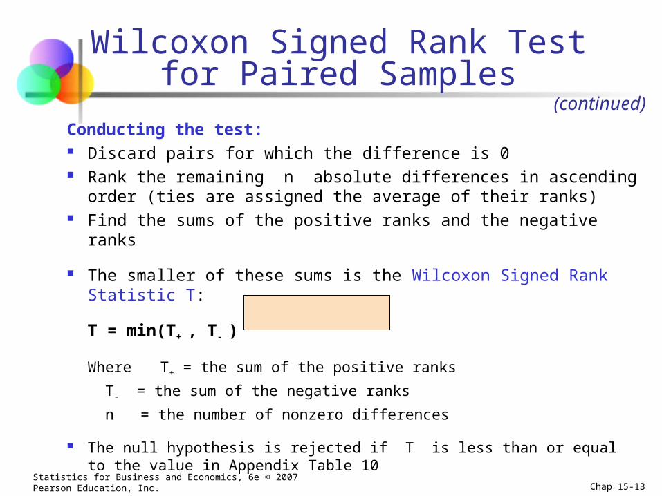
Conducting the test: Discard pairs for which the difference is 0 Rank the remaining n absolute differences in ascending order
(ties are assigned the average of their ranks) Find the sums of the positive ranks and the negative ranks
The smaller of these sums is the Wilcoxon Signed Rank Statistic T:
T = min(T+ , T- )
Where T+ = the sum of the positive ranks
T- = the sum of the negative ranks
n = the number of nonzero differences
The null hypothesis is rejected if T is less than or equal to the value in Appendix Table 10
Wilcoxon Signed Rank Test for Paired Samples
(continued)
Statistics for Business and Economics, 6e © 2007 Pearson Education, Inc. Chap 15-14
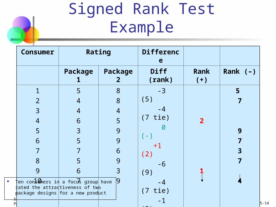
Signed Rank Test Example
T+ = 3 T– = 42
Consumer Rating Difference
Package 1 Package 2 Diff (rank) Rank (+) Rank (–)
1
2
3
4
5
6
7
8
9
10
5
4
4
6
3
5
7
5
6
7
8
8
4
5
9
9
6
9
3
9
-3 (5)
-4 (7 tie)
0 (-)
+1 (2)
-6 (9)
-4 (7 tie)
-1 (3)
-4 (7 tie)
+3 (1)
-2 (4)
2
1
5
7
9
7
3
7
4
Ten consumers in a focus group have rated the attractiveness of two package designs for a new product
Statistics for Business and Economics, 6e © 2007 Pearson Education, Inc. Chap 15-15
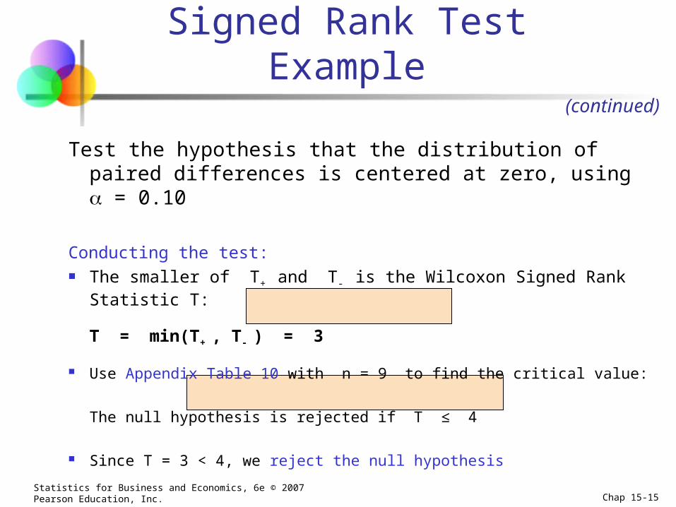
Test the hypothesis that the distribution of paired differences is centered at zero, using = 0.10
Conducting the test: The smaller of T+ and T- is the Wilcoxon Signed Rank Statistic T:
T = min(T+ , T- ) = 3
Use Appendix Table 10 with n = 9 to find the critical value:
The null hypothesis is rejected if T ≤ 4
Since T = 3 < 4, we reject the null hypothesis
(continued)
Signed Rank Test Example
Statistics for Business and Economics, 6e © 2007 Pearson Education, Inc. Chap 15-16
Wilcoxon Signed Rank Test Normal Approximation
A normal approximation can be used when
Paired samples are observed
The sample size is large
The hypothesis test is that the population distribution of differences is centered at zero
Statistics for Business and Economics, 6e © 2007 Pearson Education, Inc. Chap 15-17
The table in Appendix 10 includes T values
only for sample sizes from 4 to 20
The T statistic approaches a normal distribution as sample size increases
If the number of paired values is larger than 20, a normal approximation can be used
Wilcoxon Signed Rank Test Normal Approximation
(continued)
Statistics for Business and Economics, 6e © 2007 Pearson Education, Inc. Chap 15-18
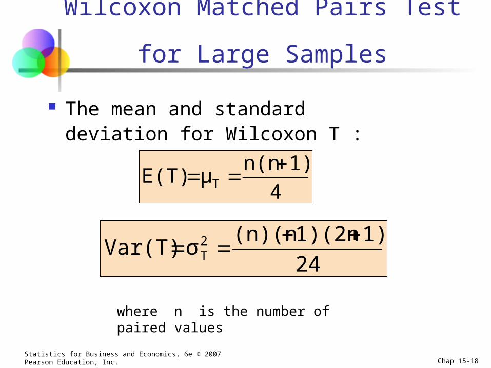
The mean and standard deviation for Wilcoxon T :
4
1)n(nμE(T) T
24
1)1)(2n(n)(nσVar(T) 2
T
where n is the number of paired values
Wilcoxon Matched Pairs Test for Large Samples
Statistics for Business and Economics, 6e © 2007 Pearson Education, Inc. Chap 15-19
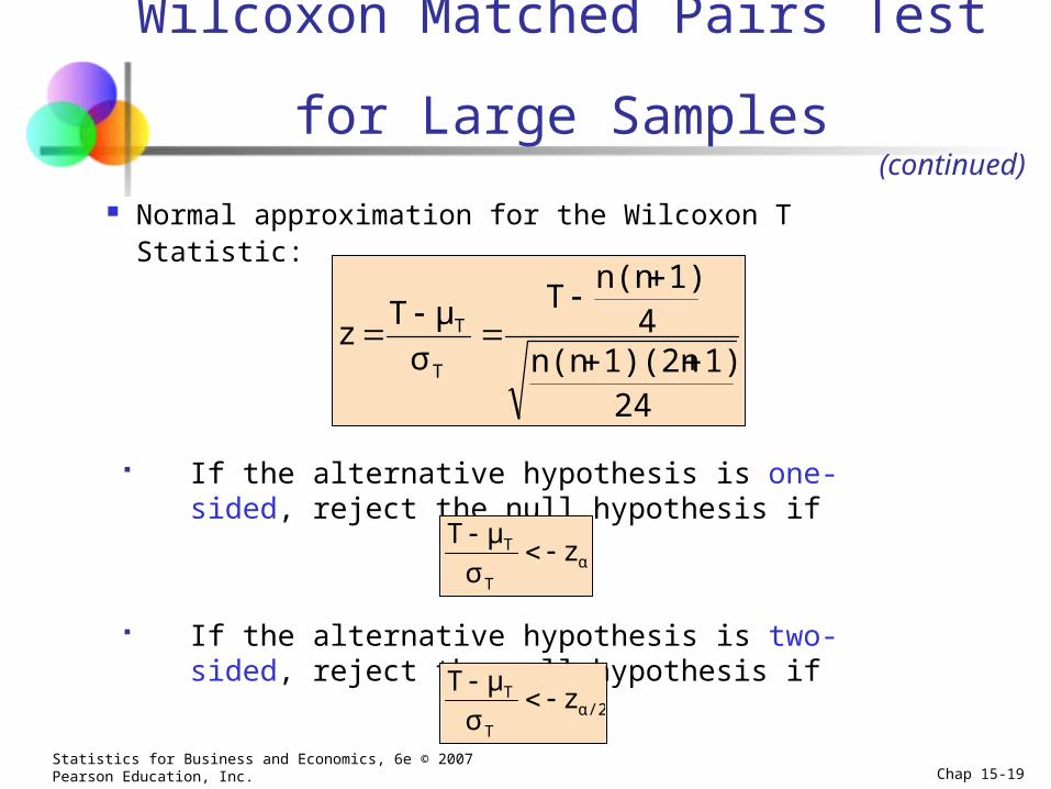
Normal approximation for the Wilcoxon T Statistic:
(continued)
241)1)(2nn(n
41)n(n
T
σ
μTz
T
T
If the alternative hypothesis is one-sided, reject the null hypothesis if
If the alternative hypothesis is two-sided, reject the null hypothesis if
αT
T zσ
μT
α/2T
T zσ
μT
Wilcoxon Matched Pairs Test for Large Samples
Statistics for Business and Economics, 6e © 2007 Pearson Education, Inc. Chap 15-20
Mann-Whitney U-Test
Used to compare two samples from two populations
Assumptions: The two samples are independent and random The value measured is a continuous variable The two distributions are identical except for a possible
difference in the central location The sample size from each population is at least 10
Statistics for Business and Economics, 6e © 2007 Pearson Education, Inc. Chap 15-21
Consider two samples Pool the two samples (combine into a singe list) but
keep track of which sample each value came from rank the values in the combined list in ascending
order For ties, assign each the average rank of the tied values
sum the resulting rankings separately for each sample
If the sum of rankings from one sample differs enough from the sum of rankings from the other sample, we conclude there is a difference in the population medians
Mann-Whitney U-Test(continued)
Statistics for Business and Economics, 6e © 2007 Pearson Education, Inc. Chap 15-22
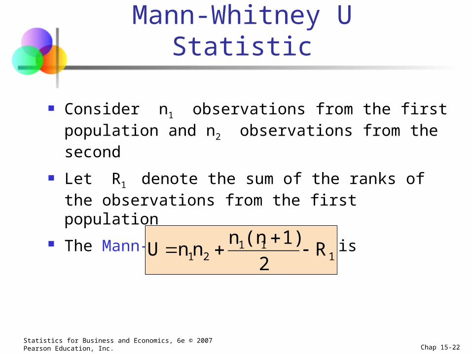
Mann-Whitney U Statistic
Consider n1 observations from the first population and n2 observations from the second
Let R1 denote the sum of the ranks of the observations from the first population
The Mann-Whitney U statistic is
111
21 R2
1)(nnnnU
Statistics for Business and Economics, 6e © 2007 Pearson Education, Inc. Chap 15-23
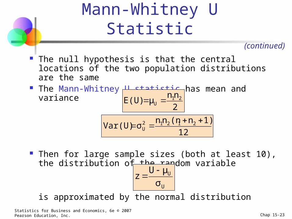
Mann-Whitney U Statistic
The null hypothesis is that the central locations of the two population distributions are the same
The Mann-Whitney U statistic has mean and variance
Then for large sample sizes (both at least 10), the distribution of the random variable
is approximated by the normal distribution
(continued)
2
nnμE(U) 21
U
12
1)n(nnnσVar(U) 21212
U
U
U
σ
μUz
Statistics for Business and Economics, 6e © 2007 Pearson Education, Inc. Chap 15-24
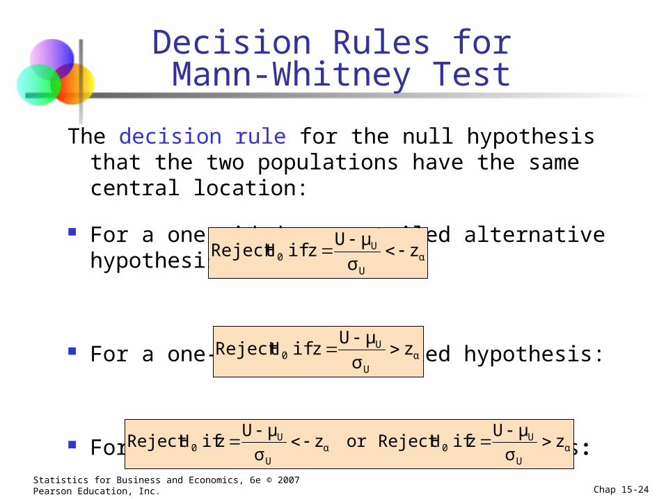
Decision Rules for Mann-Whitney Test
The decision rule for the null hypothesis that the two populations have the same central location:
For a one-sided upper-tailed alternative hypothesis:
For a one-sided lower-tailed hypothesis:
For a two-sided alternative hypothesis:
αU
U0 z
σ
μUz if H Reject
αU
U0 z
σ
μUz if H Reject
αU
U0α
U
U0 z
σ
μUz if H Rejectorz
σ
μUz if H Reject
Statistics for Business and Economics, 6e © 2007 Pearson Education, Inc. Chap 15-25
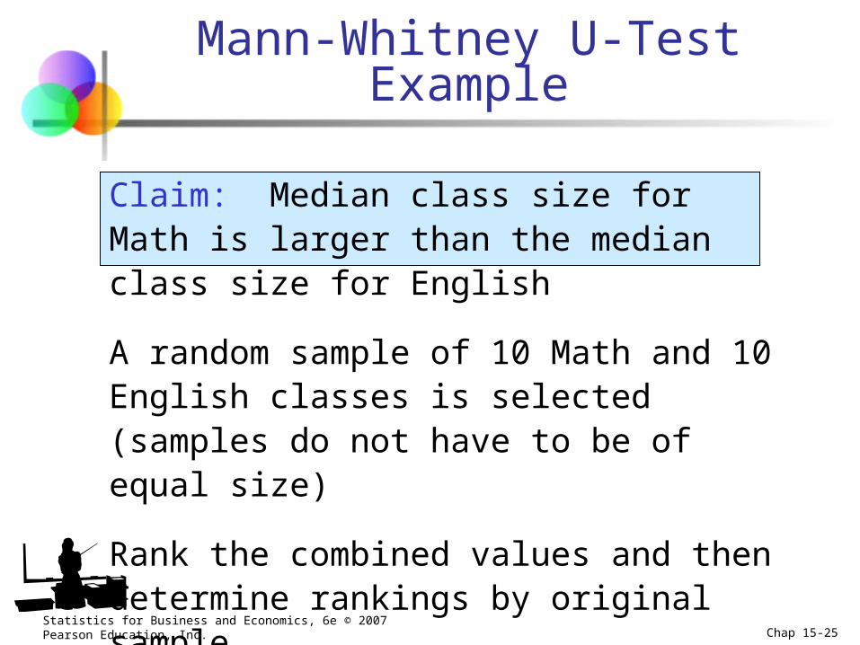
Mann-Whitney U-Test Example
Claim: Median class size for Math is larger than the median class size for English
A random sample of 10 Math and 10 English classes is selected (samples do not have to be of equal size)
Rank the combined values and then determine rankings by original sample
Statistics for Business and Economics, 6e © 2007 Pearson Education, Inc. Chap 15-26
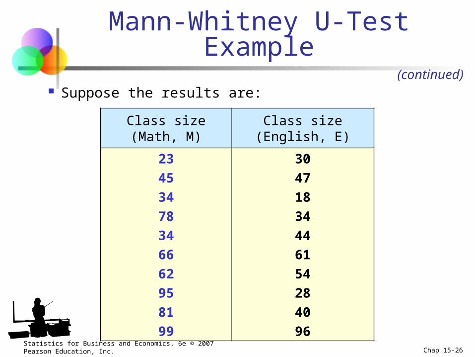
Suppose the results are:
Class size (Math, M) Class size (English, E)
23
45
34
78
34
66
62
95
81
99
30
47
18
34
44
61
54
28
40
96
(continued)
Mann-Whitney U-Test Example
Statistics for Business and Economics, 6e © 2007 Pearson Education, Inc. Chap 15-27
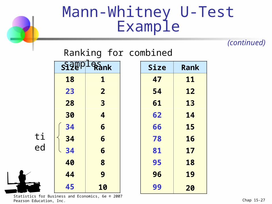
Size Rank
18 1
23 2
28 3
30 4
34 6
34 6
34 6
40 8
44 9
45 10
Size Rank
47 11
54 12
61 13
62 14
66 15
78 16
81 17
95 18
96 19
99 20
Ranking for combined samples
tied
(continued)
Mann-Whitney U-Test Example
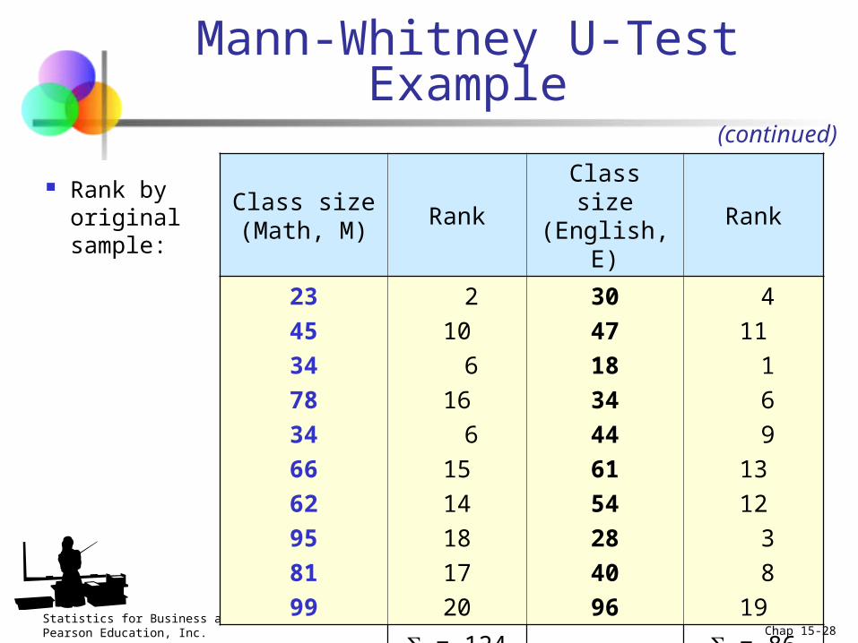
Statistics for Business and Economics, 6e © 2007 Pearson Education, Inc. Chap 15-28
Rank by original sample:
Class size (Math, M)
RankClass size
(English, E)Rank
23
45
34
78
34
66
62
95
81
99
2
10
6
16
6
15
14
18
17
20
30
47
18
34
44
61
54
28
40
96
4
11
1
6
9
13
12
3
8
19
= 124 = 86
(continued)
Mann-Whitney U-Test Example
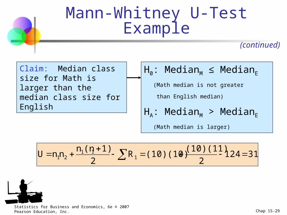
Statistics for Business and Economics, 6e © 2007 Pearson Education, Inc. Chap 15-29
H0: MedianM ≤ MedianE
(Math median is not greater
than English median)
HA: MedianM > MedianE
(Math median is larger)
Claim: Median class size for Math is larger than the median class size for English
311242
(10)(11)(10)(10)R
2
1)(nnnnU 1
1121
(continued)
Mann-Whitney U-Test Example
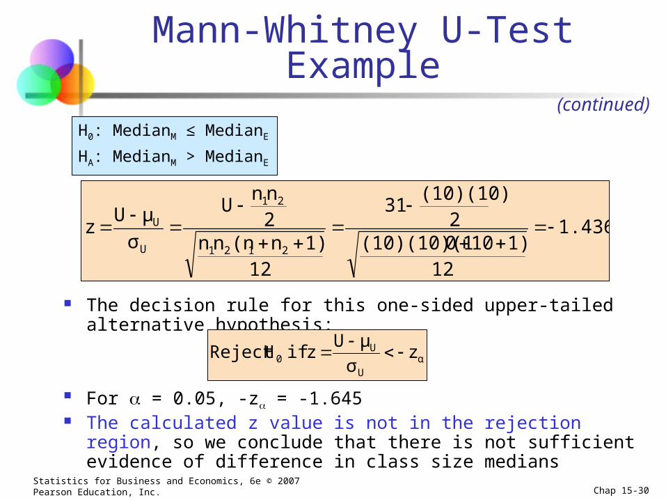
Statistics for Business and Economics, 6e © 2007 Pearson Education, Inc. Chap 15-30
(continued)
1.436
121)100(10)(10)(1
2(10)(10)
31
121)n(nnn
2nn
U
σ
μUz
2121
21
U
U
Mann-Whitney U-Test Example
H0: MedianM ≤ MedianE
HA: MedianM > MedianE
The decision rule for this one-sided upper-tailed alternative hypothesis:
For = 0.05, -z = -1.645 The calculated z value is not in the rejection region, so we
conclude that there is not sufficient evidence of difference in class size medians
αU
U0 z
σ
μUz if H Reject
Statistics for Business and Economics, 6e © 2007 Pearson Education, Inc. Chap 15-31
Wilcoxon Rank Sum Test
Similar to Mann-Whitney U test
Results will be the same for both tests
Statistics for Business and Economics, 6e © 2007 Pearson Education, Inc. Chap 15-32
Wilcoxon Rank Sum Test
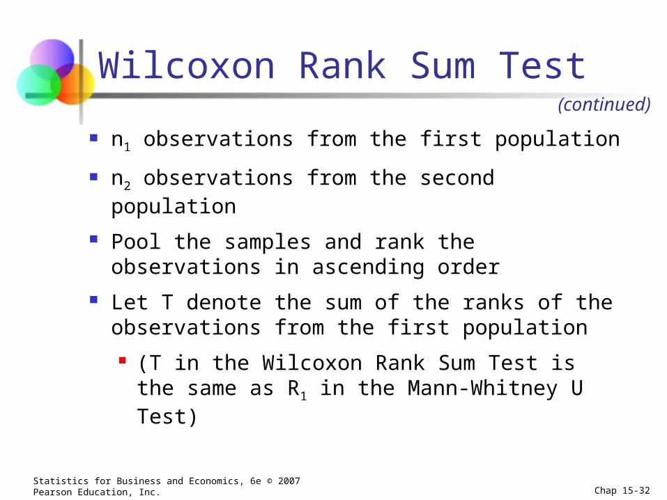
n1 observations from the first population
n2 observations from the second population
Pool the samples and rank the observations in ascending order
Let T denote the sum of the ranks of the observations from the first population
(T in the Wilcoxon Rank Sum Test is the same as R1 in the Mann-Whitney U Test)
(continued)
Statistics for Business and Economics, 6e © 2007 Pearson Education, Inc. Chap 15-33
Wilcoxon Rank Sum Test
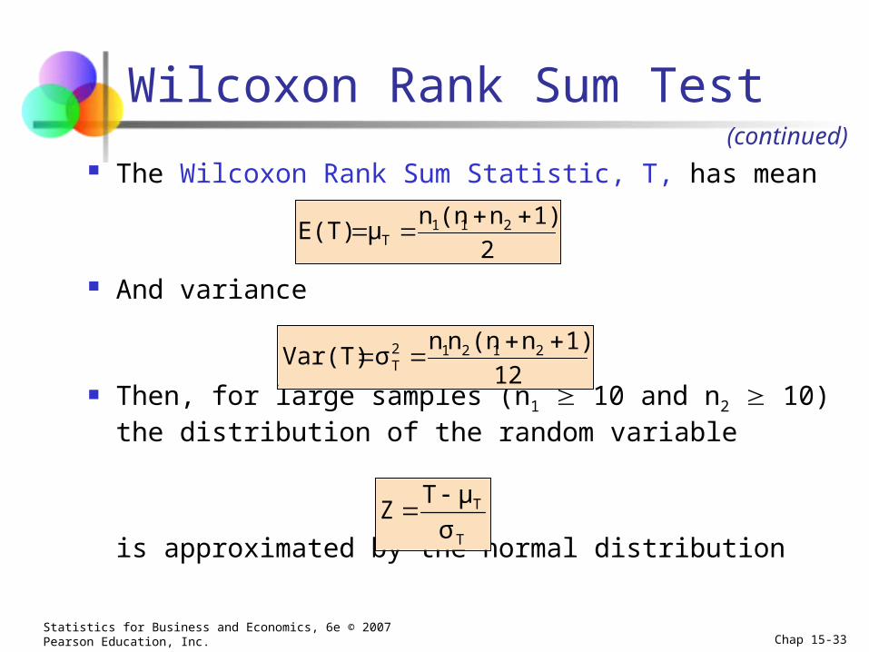
The Wilcoxon Rank Sum Statistic, T, has mean
And variance
Then, for large samples (n1 10 and n2 10) the distribution of the random variable
is approximated by the normal distribution
(continued)
2
1)n(nnμE(T) 211
T
12
1)n(nnnσVar(T) 21212
T
T
T
σ
μTZ
Statistics for Business and Economics, 6e © 2007 Pearson Education, Inc. Chap 15-34
Wilcoxon Rank Sum Example
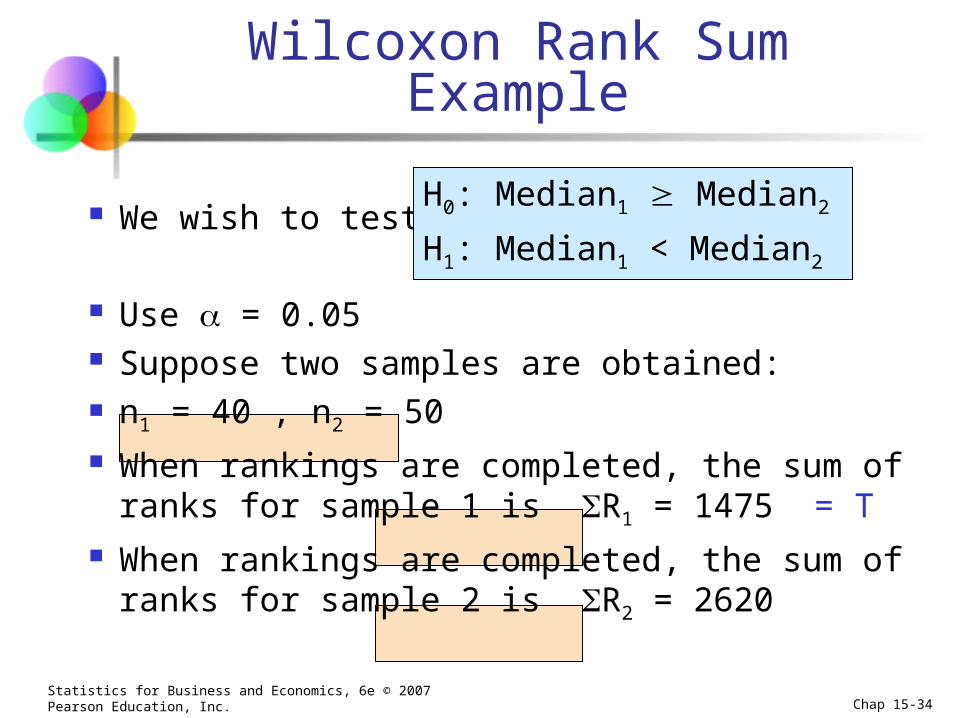
We wish to test
Use = 0.05 Suppose two samples are obtained: n1 = 40 , n2 = 50 When rankings are completed, the sum of ranks
for sample 1 is R1 = 1475 = T When rankings are completed, the sum of ranks
for sample 2 is R2 = 2620
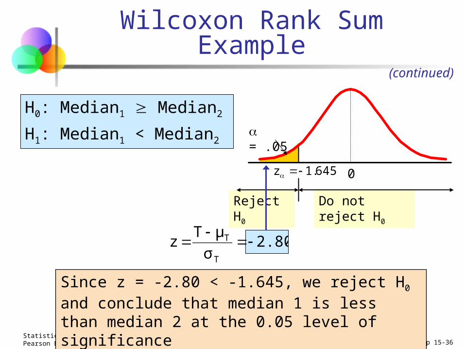
H0: Median1 Median2
H1: Median1 < Median2
Statistics for Business and Economics, 6e © 2007 Pearson Education, Inc. Chap 15-35
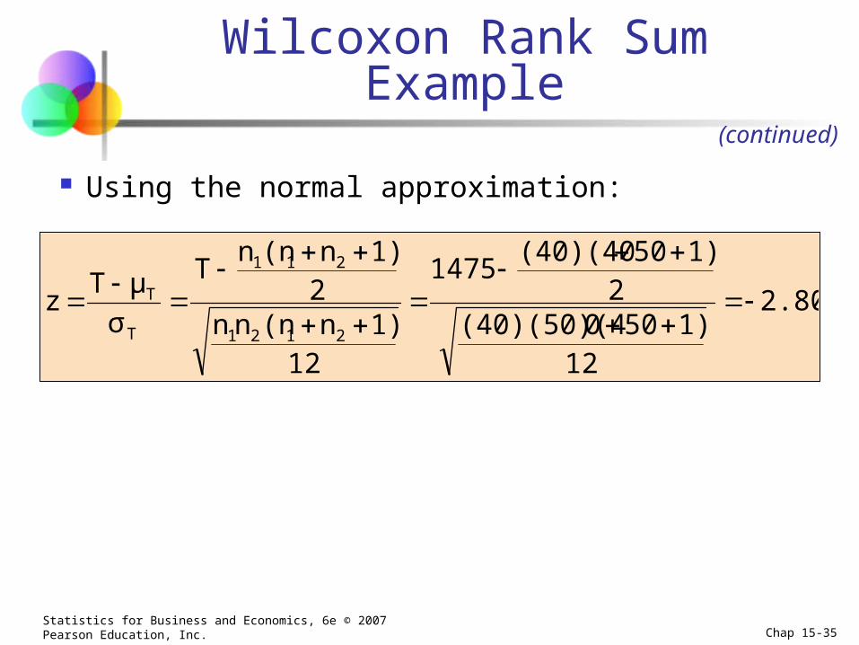
Using the normal approximation:
(continued)
Wilcoxon Rank Sum Example
2.80
121)500(40)(50)(4
21)50(40)(40
1475
121)n(nnn
21)n(nn
T
σ
μT z
2121
211
T
T
Statistics for Business and Economics, 6e © 2007 Pearson Education, Inc. Chap 15-36
Since z = -2.80 < -1.645, we reject H0 and conclude that median 1 is less than median 2 at the 0.05 level of significance
645.1z
Reject H0
= .05
Do not reject H0
0
(continued)
Wilcoxon Rank Sum Example
2.80σ
μT z
T
T
H0: Median1 Median2
H1: Median1 < Median2
Statistics for Business and Economics, 6e © 2007 Pearson Education, Inc. Chap 15-37
Spearman Rank Correlation
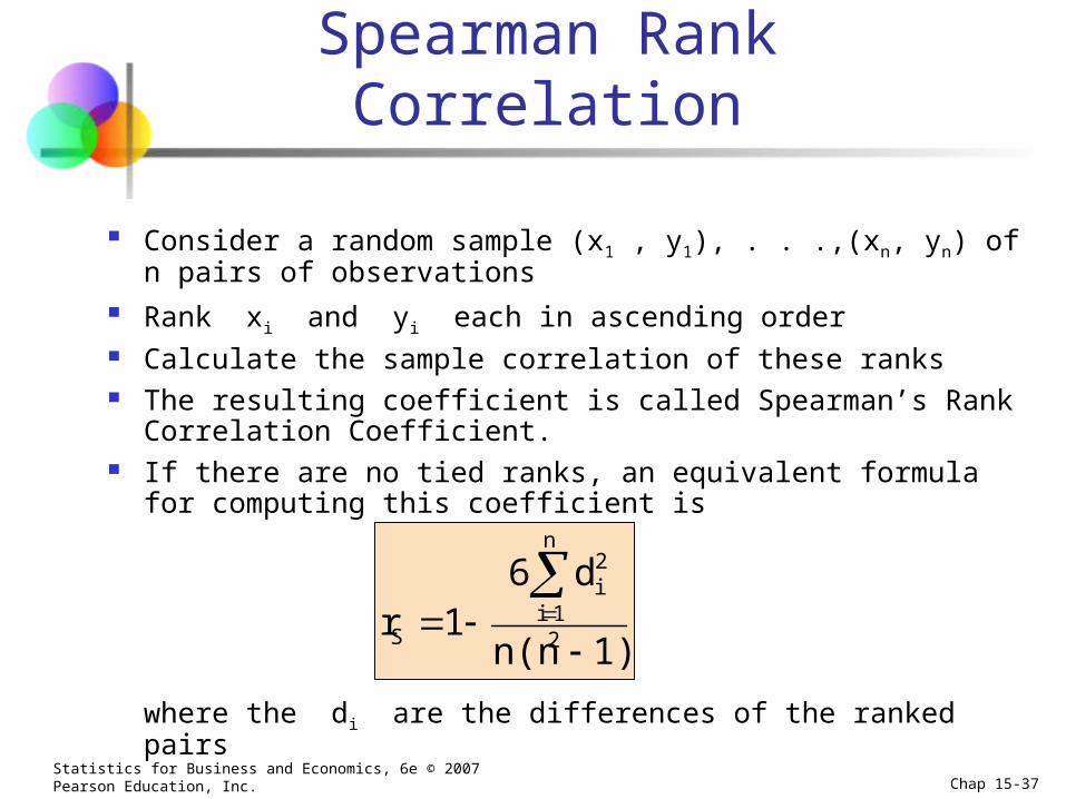
Consider a random sample (x1 , y1), . . .,(xn, yn) of n pairs of observations
Rank xi and yi each in ascending order Calculate the sample correlation of these ranks The resulting coefficient is called Spearman’s Rank Correlation
Coefficient. If there are no tied ranks, an equivalent formula for computing this
coefficient is
where the di are the differences of the ranked pairs
1)n(n
d61r
2
n
1i
2i
S
Statistics for Business and Economics, 6e © 2007 Pearson Education, Inc. Chap 15-38
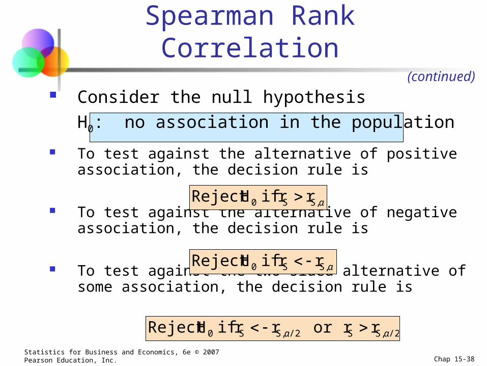
Consider the null hypothesis
H0: no association in the population
To test against the alternative of positive association, the decision rule is
To test against the alternative of negative association, the decision rule is
To test against the two-sided alternative of some association, the decision rule is
Spearman Rank Correlation(continued)
αS,S0 rr if H Reject
αS,S0 rr if H Reject
/2S,S/2S,S0 rrorrr if H Reject αα
Statistics for Business and Economics, 6e © 2007 Pearson Education, Inc. Chap 15-39
Chapter Summary
Used the sign test for paired or matched samples, and the normal approximation for the sign test
Developed and applied the Wilcoxon signed rank test, and the large sample normal approximation
Developed and applied the Mann-Whitney U-test for two population medians
Used the Wilcoxon rank-sum test
Examined Spearman rank correlation for tests of association