HAL Id: hal-00813015https://hal.archives-ouvertes.fr/hal-00813015

Submitted on 31 May 2013

HAL is a multi-disciplinary open accessarchive for the deposit and dissemination of sci-entific research documents, whether they are pub-lished or not. The documents may come fromteaching and research institutions in France orabroad, or from public or private research centers.

L’archive ouverte pluridisciplinaire HAL, estdestinée au dépôt et à la diffusion de documentsscientifiques de niveau recherche, publiés ou non,émanant des établissements d’enseignement et derecherche français ou étrangers, des laboratoirespublics ou privés.

Cerebrospinal fluid volume analysis for hydrocephalusdiagnosis and clinical research

Alain Lebret, Jérôme Hodel, Alain Rahmouni, Philippe Decq, Eric Petit

To cite this version:Alain Lebret, Jérôme Hodel, Alain Rahmouni, Philippe Decq, Eric Petit. Cerebrospinal fluid volumeanalysis for hydrocephalus diagnosis and clinical research. Computerized Medical Imaging and Graph-ics, Elsevier, 2013, 37 (3), pp.224-233. <10.1016/j.compmedimag.2013.03.005>. <hal-00813015>

Cerebrospinal fluid volume analysis for hydrocephalus diagnosis

and clinical research

Alain Lebreta, Jerome Hodelb, Alain Rahmounic, Philippe Decqc, Eric Petita

aUniversite Paris-Est, LISSI (EA 3956), UPEC, F-94010, Creteil, FrancebHopital Saint-Joseph, 185 Rue Raymond Losserand, F-75014, Paris, France

cHopital Henri Mondor, 51 Av du Marechal de Lattre de Tassigny, F-94010, Creteil, France

Abstract

In this paper we analyze volumes of the cerebrospinal fluid spaces for the diagnosis of hy-drocephalus, which are served as reference values for future studies. We first present anautomatic method to estimate those volumes from a new three-dimensional whole bodymagnetic resonance imaging sequence. This enables us to statistically analyze the fluidvolumes, and to show that the ratio of subarachnoid volume to ventricular one is a propor-tionality constant for healthy adults (= 10.73), while in range [0.63, 4.61] for hydrocephaluspatients. This indicates that a robust distinction between pathological and healthy casescan be achieved by using this ratio as an index.

Keywords: cerebrospinal fluid, hydrocephalus, volume assessment, three-dimensionalimage analysis, computer-aided diagnosis

1. Introduction

Hydrocephalus is a neurological disorder involving an abnormal accumulation of thecerebrospinal fluid in the cavities of the brain known as cerebral ventricles. The centralnervous system is completely surrounded by the fluid contained within these ventricles andthe subarachnoid space. A ventricle enlargement will increase pressure on the brain, whichcan result in damage to brain tissues and several brain malfunctions. The fluid circulatesfrom ventricles where it is produced to the subarachnoid space where it is resorbed intothe circulatory system [1]. Figure 1 shows descriptive representations of the fluid pathwayfrom ventricles to the subarachnoid space in a sagittal plane (left) and through the variousencountered spaces as proposed in [2] (right). Hydrocephalus can be classified into non-communicating and communicating depending on whether the fluid pathway is obstructedor not [2]. The common test to diagnose hydrocephalus is requiring imaging techniques, suchas computed tomography, magnetic resonance imaging, or pressure monitoring techniques inorder to identify the enlarged ventricles and any obstruction in the fluid pathway. In routineclinical practice, those techniques are mainly limited to the intracranial region and may need

Email address: Alain-Rene.Lebret@ac-paris.fr (Alain Lebret)

1

BRAIN

Lateral ventricle

3rd ventricle

4th ventricle

Subarachnoid space

Lateralventricles

3rd ventricle

Cerebral aqueduct

4th ventricle

Ventricularspace

Cortical + Spinalsubarachnoidspace

CSF

Figure 1: The cerebrospinal fluid circulates from ventricles where it is produced to the subarachnoidspace where it is resorbed (left). The fluid flows through the various encountered spaces from theventricles to the cortical subarachnoid space as proposed in [2] (right).

different sequences to identify the enlargement and highlight an obstruction. For instance,a ventricle enlargement can be identified by a magnetic resonance imaging sequence, whiledetecting a fluid flow malfunction may require an additional cine phase-contrast magneticresonance imaging sequence.

Several papers have suggested a cerebrospinal fluid volume assessment to characterizehydrocephalus. For instance, a quantification is performed for healthy volunteers and pa-tients with various types of hydrocephalus in [3, 4], whereas it is limited to normal pressurehydrocephalus, i.e. a specific case of communicating hydrocephalus in [5]. Nevertheless, allof them are restricted to the intracranial region, while it is assumed that the spinal sub-arachnoid space volume may also provide some information in hydrocephalus analysis [6].Images reveal most cerebral structures, which do not facilitate segmentation of the fluiditself in a routine way. Thus, there is not yet any whole body method that is routinely used.

The aim of this work is to provide both a method to assess volumes of the entire cere-brospinal fluid in order to diagnose hydrocephalus and reference values for future studies.We have recently developed a new magnetic resonance imaging sequence that significantlyhighlights the cerebrospinal fluid [7] and proposed an automatic segmentation of its entirevolume in [8]. To quantify the fluid volumes from those whole body images, we propose inthis paper to improve the method described in [8] by automatically separating the entirefluid volume into its spinal subarachnoid, cortical subarachnoid and ventricular spaces. Wealso show the ability of our volume assessment to be exploited to perform statistical analy-ses, which lead to a functional parameter calculated by the ratio of the entire subarachnoidspace volume to the ventricular one. We assume this parameter could be efficient to dis-

2

criminate healthy adults from patients affected by communicating and non-communicatinghydrocephalus. Furthermore, our approach only requires a single imaging sequence and anautomatic image processing for each patient.

Concerning our segmentation method, we should consider the complex geometry of thecerebrospinal shape and its human variability, the presence of noise and artifacts, especiallymotion artifacts, and the possible obstructed fluid pathway, which results in a disconnec-tion of the fluid spaces in non-communicating hydrocephalus cases. To overcome theseproblems, we introduce a topological assumption on the entire cerebrospinal fluid shape.This property, used as a refinement constraint, brings both accuracy and robustness to oursegmentation method, particularly for pathological cases. The separation method of thepreviously segmented total fluid volume involves a region of interest defined from eyeballs.Spinal and intracranial spaces are separated by detecting a topological change of the fluidin the bottom part of the region of interest. Then, the ventricular space is separated fromthe intracranial space by reconstructing the ventricles from a specific tubular structure. Allthese steps are configured with default values that we specified, and can be chained withoutrequiring any user interaction. Some steps may be even parallelized (e.g. the two separationmethods).

This paper is organized as follows. Section 2 describes the segmentation method forthe entire cerebrospinal fluid volume assessment. The separation of the entire volume intoits ventricular and subarachnoid volumes is presented in Section 3. In Section 4, we firstevaluate our volume assessment and then make statistical analyses on our clinical dataset,such as linear regression and linear discriminant analysis. Concluding remarks are given inSection 5.

2. Segmentation of the entire cerebrospinal fluid

Our input whole body images appear to be binary due to the poor dynamic of theluminance perception of the human visual system but in fact they are not (see Fig. 2-a).Furthermore, images are disturbed by noise and artifacts. We thus use image properties anda topological assumption on the fluid shape for segmenting the entire cerebrospinal fluidvolume.

2.1. Topological model of the cerebrospinal fluid

Topology is the mathematical study of spatial objects that are preserved through de-formations such as twistings and stretchings, without regarding to their size and position.Properties of objects are considered by abstracting their inherent connectivities while ig-noring their detailed shapes. More details on topology for digital images may be found inChapter 6 of [9].

Numerous studies have demonstrated the effectiveness to integrate such topological con-straints in medical image processing (see [10] for an overview). For instance, most brainstructures have the topology of a filled or hollow sphere while their geometry is complex.We consider the entire fluid to be topologically equivalent to a filled sphere that is compliantwith the fluid flow as shown in Fig. 1, while many people use rather a hollow sphere (or

3

a more complex object) as its topological model [11, 12, 13]. Models closest to the reality[11, 13] are well adapted to address problems such as surface correction. However, our as-sumption significantly simplifies and also speeds up the initialization step compared to thatof a hollow sphere, while the difference between the two resulting volumes is negligible. Fur-thermore, it introduces neither unexpected cavity nor handle despite of noise and artifacts,and is also more efficient and consistent for hydrocephalus patients for whom the fluid donot fit a hollow sphere anymore.

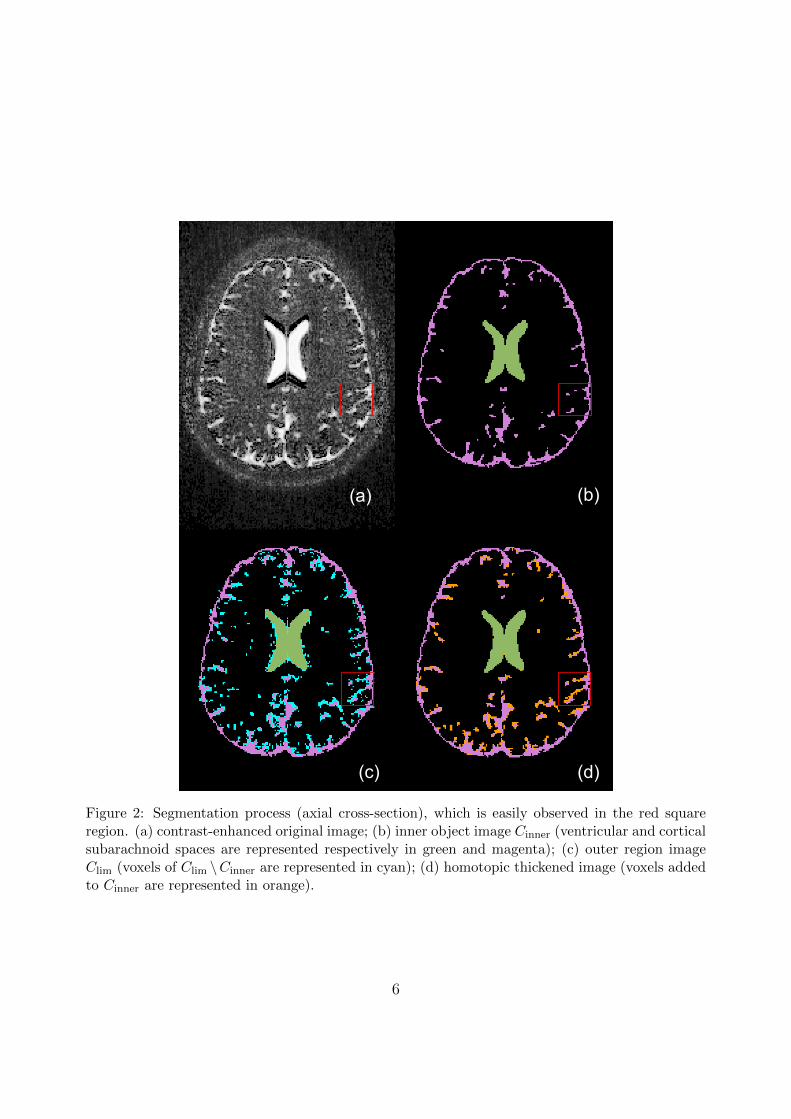
2.2. Segmentation of the entire cerebrospinal fluid volumeSegmentation consists in homotopically thicken an inner object (Cinner), which is within

the entire cerebrospinal fluid and is topologically equivalent to a filled sphere. This trans-formation, which preserves the topology of the inner object, is guided by a priority functionbased on a distance criterion. The inner object can be interactively or automatically defined,as long as it has the correct topology.

To significantly speed up the processing time, we propose to automatically initialize theinner object as close as possible to the border of the cerebrospinal fluid. We also initializean outer object of the cerebrospinal fluid (Clim), which includes the entire fluid but do notnecessarily have the same topology. Thus, guiding the thickening by the priority function islimited to the region between Cinner and Clim.

2.2.1. Initialization of inner and outer objects

An inner object Cinner is initialized by applying the moment-preserving thresholding de-scribed in [14] on the initial image, followed by a larger connected component extraction(Fig. 2b). The moment-preserving thresholding is suited to “binary nature” images withlow contrast. The moment preservation assumes that statistical moments on initial andthresholded images are identical. This method becomes more efficient than conventionalclustering-based or entropy-based methods when the histogram presents an excessive over-lapping between classes. Since the thresholded image contains several objects, a connectedcomponent labeling [15] is performed to extract the three largest connected components,which generally correspond to the inner object Cinner and both eyeballs E1 and E2. E1 andE2 are retained to determine a region of interest in Section 3.1. By extracting the largestcomponents, residual noise as well as other small objects such as salivary ducts are alsoremoved. If Cinner has holes, (see [9, Section 5.3.3] for a hole characterization) then thethreshold is automatically adjusted by increasing its value until the topological assumptionon Cinner is satisfied; E1 and E2 are not affected by this operation due to their intensity.

To initialize an outer object Clim, another histogram-based thresholding method is carriedout on the initial image as described in [16]. The triangle thresholding algorithm in [16] issuitable for bimodal images for which the object to extract has a small amplitude and alarge variance relatively to the background. It is followed by a largest connected componentextraction to retrieve an outer object of the fluid (Clim) as shown in Fig. 2c.

2.2.2. Priority function

The priority function Ψ = {ψx} controls the order in which voxels are processed andeventually added to Cinner. This function uses an Euclidean distance map denoted by D =

4

{dx}, which is defined for each voxel x ∈ C inner as the distance to the nearest voxel of Cinner;it is calculated by the linear algorithm proposed in [17]. The value ψx of each voxel x in theouter object Clim is then given by:

ψx =

{dx if x ∈ Clim,

+∞ otherwise.(1)

Euclidean distance transform was preferred to others because it improves selection of pointsthat should be tested while the thickening process.

2.2.3. Guided homotopic thickening

Guided by the previous priority function Ψ, an homotopic thickening is applied to theinner object Cinner by adding simple points.

A point is simple if its addition to or its removal from a binary object C does not changethe topology of the object and of the background. Therefore, removing simple points doesnot change the number of connected components and holes (cavities and/or handles) of Cand its complement C. It is shown in [18] that a simple point x is locally characterized bytwo local topological numbers. An efficient computation of these numbers that only involvesthe 26-neighborhood is also described in [18].

Let ∂C inner denote the boundary of Cinner such that ∂C inner = {x ∈ C inner ∩ Clim |N6(x) ∩Cinner 6= ∅}, where N6(x) is the 6–neighborhood of x. The thickening process consists inadding to Cinner simple points from ∂C inner as presented in Algorithm 1. It shows thatboundary points (i.e. voxels) of ∂C inner are chosen iteratively, according to their priorities,and are incorporated into Cinner if they are simple.

Algorithm 1: Guided homotopic thickening

Input: Cinner, ΨOutput: Cinner

Initialize ∂C inner ;Make a priority queue Q of all x ∈ ∂C inner using ψx in the ascending order ;while Q 6= ∅ do

Poll x from Q ;if x is simple for Cinner thenCinner ← Cinner ∪ {x} ;Modify ∂C inner ;Insert new points of ∂C inner around x to Q ;

end ifend while

The resulting thickened object has the same topology as Cinner. It is illustrated in Fig. 2d.

5

(b)(a)

(c) (d)

Figure 2: Segmentation process (axial cross-section), which is easily observed in the red squareregion. (a) contrast-enhanced original image; (b) inner object image Cinner (ventricular and corticalsubarachnoid spaces are represented respectively in green and magenta); (c) outer region imageClim (voxels of Clim \Cinner are represented in cyan); (d) homotopic thickened image (voxels addedto Cinner are represented in orange).

6

3. Separation into cerebrospinal fluid volumes

Separation of the cerebrospinal fluid spaces is required to analyze the relationship be-tween the entire subarachnoid and ventricular volumes. First, the spinal and intracranialregions are separated using a topological property of the cerebrospinal fluid at their interface.Second, to retrieve the volume of the ventricular space from that of the cortical subarach-noid one, the cerebral aqueduct must be detected because we use it as a morphologicalreconstruction marker.

3.1. Separation of spinal and intracranial spaces

Expert physicians usually perform the disconnection of the spinal and intracranial spacesby tracking the foramen magnum (the hole in the bottom of the skull through which thespinal cord passes in order to be connected to the brain), which is, even for an expert,difficult to detect on this type of image. The separation into spinal and intracranial spacesrequires to locate the closest axial cross-section plane to that of the foramen magnum. Thus,the disconnection is achieved by browsing the planar connected component on each axialplane from the spinal part, and by detecting any change in its topology (see the axial cross-section in Fig. 3). A region of interest is first determined to reduce the processing time aswell as to improve the robustness.

3.1.1. Determination of the region of interest

A region of interest R is used to retrieve the cerebral aqueduct in order to separatethe intracranial space into its ventricular and subarachnoid spaces (Section 3.2). Apartfrom pathological cases, eyeballs typically face the cerebral aqueduct in the axial plane. Weconsider the region forming a rectangular cuboid, each of whose edge is parallel to one ofthe i-, j-, k-axes of the image, such that:

• the region is located in the i-axis direction between the coronal plane that passesthrough the maximum posterior boundary of eyeballs, and the last coronal plane thatstill contains non-zero voxels;

• setting D as the larger diameter of both eyeballs, the height of the region is set em-pirically to be 8D, such that the top face of the region is located with the distance2D above the eyeballs and the bottom face is located with the distance 5D below theeyeballs. The height is chosen in agreement with an expert so as to contain all thenecessary structures for the separation step. It may also be interactively resized to fithuman variations;

• the depth is determined by the two sagittal planes between the medial boundaries ofeyeballs.

3.1.2. Determination of the cut-off plane

Planar connected components are counted on each axial plane from the bottom to thetop of the region of interest R. The first axial plane that shows a change in the number ofconnected components is the plane just above that of the searched cut-off (Fig. 3).

7

cut-off plane

FM plane

z = 173 z = 172 z = 171

z = 170 z = 169 z = 168

z = 167 z = 166 z = 165

R

Figure 3: Separation of intracranial and spinal regions in the region of interest R. The resultingcut-off plane (z = 166) is close to that goes through the foramen magnum (FM plane). The axialcross-sections around the cut-off plane are also illustrated (right).

1

infundibular recess

2

Figure 4: Proximity of the interpeduncular cistern (1) to the infundibular recess of the thirdventricle (2). The small rectangular part in the left figure is zoomed in the right figure.

3.2. Intracranial volume separation

The process to extract the ventricular space may fail because of some subarachnoidregions that are very close to the third and fourth ventricles. Figure 4 shows, for instance,the proximity between the interpeduncular cistern and the infundibular recess of the thirdventricle.

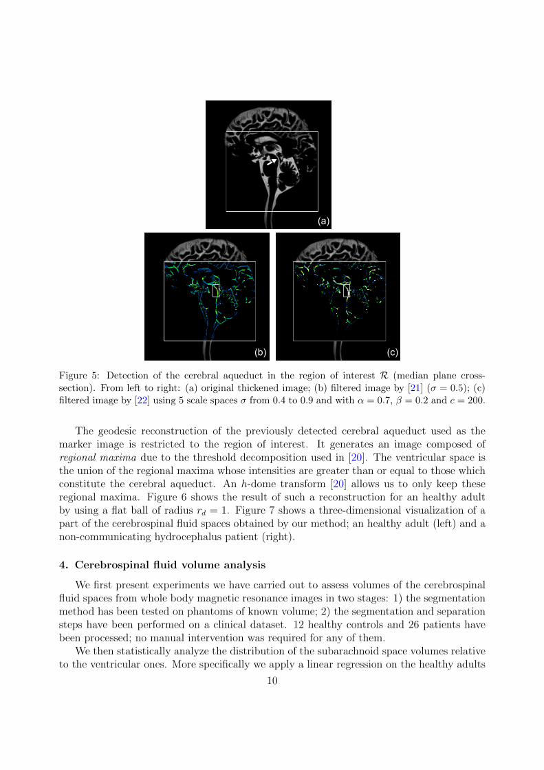
To overcome this problem we first detect the cerebral aqueduct that is a thin tubularstructure (diameter: 1 to 3 mm; length: around 14 mm) located in the median sagittal plane,which connects the third and fourth ventricles. It is also the longest tubular structure withthe highest intensity range in the most median sagittal planes of the region of interest R. Itsenhancement is performed by a vessel segmentation method (see [19]). Finally, ventricles arerecovered by a morphological reconstruction [20] using the cerebral aqueduct as a marker.

3.2.1. Detection of the cerebral aqueduct

Several methods to enhance vessel like structures in grayscale images are reviewed in[19]. Several efficient methods are based on properties of eigenvalues of the Hessian matrix

8

H [21, 22]. These multi-scale methods operate in a Gaussian scale space on which theycalculate second-order derivatives, build the Hessian matrix H, and decompose it dependingon its eigenvalues λ1, λ2 and λ3 such that |λ1| < |λ2| < |λ3|. The eigenvalues are analyzed todetermine the likelihood for each voxel x to belong to a curvilinear structure. This analysisis based on the following assumptions: (1) λ1 ≈ 0; (2) λ2 ≈ λ3 < 0; and (3) |λ1| � |λ2|.

The tubular structure filter implemented in [22] allows to dissociate strict tubular struc-tures from others. We use it here to enhance the cerebral aqueduct. Let Fσ = {fσx } thefilter in [22] such that:

fσx =

{0 if λ2 > 0 or λ3 > 0,

(1− e−R2A

2α2 )e−R2

B2β2 (1− e−

S2

2c2 ) otherwise,(2)

where RA = |λ2| / |λ3|, RB = |λ1| /√|λ2λ3|, S =

√λ21 + λ22 + λ23, with some weights α ∈

[0, 1], β ∈]0, 1] and c ∈ [0, 500]. Figure 5 compares extracted curvilinear structures in theregion of interest R using methods from [21] (Fig. 5b) and [22] (Fig. 5c). It shows thatin contrast with [21], the filter in [22] allows to dissociate strict tubular structures fromothers. The cerebral aqueduct part has more highlighted values in Fig. 5c by adjusting thefilter with a higher weight to detect lines (α = 0.7). The aqueduct is the longest connectedcomponent found in the most median sagittal planes.

3.2.2. Ventricles reconstruction

Considering the cerebral aqueduct part as the marker, we aim to reconstruct the ven-tricular space. For this problem, methods such as fast marching [23], level set [23] or activecontour models [24] are well known. However, the following two problems may hinder thereconstruction by the above methods: 1) the cerebral aqueduct part is too small as a markerto initialize a model; 2) motion artifacts can generate significant intensity inhomogeneitieseven in the ventricular space.

Geodesic reconstruction [20] is a very useful operator from mathematical morphologythat provides quite satisfactory results here.

Let δ(1)f,Bd

(g) be the elementary geodesic dilation of a grayscale image g inside f (g is

called the marker image and f is the mask) such that δ(1)f,Bd

(g) = (g ⊕ Bd) ∧ f , where ∧stands for the point-wise minimum and g ⊕ Bd is the geodesic dilation of g by an isotropicstructuring element Bd chosen as a flat ball of radius rd = 1. The geodesic dilation of sizen ≥ 0 is obtained by:

δ(n)f,Bd

(g) = δ(1)f,Bd◦ δ(1)f,Bd

◦ · · · ◦ δ(1)f,Bd(g)︸ ︷︷ ︸

n times

. (3)

The grayscale reconstruction by dilation ρf,Bd(g) of f from g is calculated by iterating

geodesic dilations of g inside f until idempotence such that:

ρf,Bd(g) = ∨

n≥1δ(n)f,Bd

(g) , (4)

where ∨ stands for the point-wise maximum.

9

(a)

(b) (c)

Figure 5: Detection of the cerebral aqueduct in the region of interest R (median plane cross-section). From left to right: (a) original thickened image; (b) filtered image by [21] (σ = 0.5); (c)filtered image by [22] using 5 scale spaces σ from 0.4 to 0.9 and with α = 0.7, β = 0.2 and c = 200.

The geodesic reconstruction of the previously detected cerebral aqueduct used as themarker image is restricted to the region of interest. It generates an image composed ofregional maxima due to the threshold decomposition used in [20]. The ventricular space isthe union of the regional maxima whose intensities are greater than or equal to those whichconstitute the cerebral aqueduct. An h-dome transform [20] allows us to only keep theseregional maxima. Figure 6 shows the result of such a reconstruction for an healthy adultby using a flat ball of radius rd = 1. Figure 7 shows a three-dimensional visualization of apart of the cerebrospinal fluid spaces obtained by our method; an healthy adult (left) and anon-communicating hydrocephalus patient (right).

4. Cerebrospinal fluid volume analysis

We first present experiments we have carried out to assess volumes of the cerebrospinalfluid spaces from whole body magnetic resonance images in two stages: 1) the segmentationmethod has been tested on phantoms of known volume; 2) the segmentation and separationsteps have been performed on a clinical dataset. 12 healthy controls and 26 patients havebeen processed; no manual intervention was required for any of them.

We then statistically analyze the distribution of the subarachnoid space volumes relativeto the ventricular ones. More specifically we apply a linear regression on the healthy adults

10

(a) (b)

(c)

Figure 6: Ventricular space retrieving using a grayscale reconstruction by dilation of the cerebralaqueduct inside the original image: (a) the initial image (the mask) and the cerebral aqueduct (themarker) colored in red; (b) result of the grayscale reconstruction with regional maxima coloredin different tons of green; (c) frontal (left) and sagittal (right) views of the ventricular space foran healthy adult using a grayscale reconstruction by dilation of the cerebral aqueduct inside theregion of interest R.

subset, as well as a linear discriminant analysis on the clinical dataset distribution to classifyhealthy and pathological cases.

4.1. Volume assessment

Experiments for volume assessment were carried out on 5 phantoms of known volume(image size: 128 slices of 250× 250 in the sagittal plane) and 38 clinical images (image size:160 slices of around 260×790 in the sagittal plane). Processing took place on a conventionalPC (Intel Pentium Dual Core 1.60 GHz / 4 GB main memory, Linux 2.6 operating system).The overall time to assess volumes is 20 min or less for each patient: 12 min or less for theimage acquisition and approximately 6 min for its processing. Obviously, this computationtime could be dramatically reduced by using a computer with an architecture dedicated tothree-dimensional image processing.

4.1.1. Images acquisition

Magnetic resonance images were acquired in the sagittal plane on a 1.5 T system (Mag-netom Avanto; Siemens Medical Solutions, Erlangen, Germany). The magnetic resonance

11

Figure 7: Partial three-dimensional surface rendering (the cortical subarachnoid space was cutalong the sagittal plane). Ventricular, cortical subarachnoid and spinal subarachnoid spaces are re-spectively colored in green, magenta and cyan. Left: an healthy adult; right: a non-communicatinghydrocephalus patient.

sequence in [7], called SPACE (Sampling Perfection with Application optimized Contrastusing different flip-angle Evolution), is a variant of the T2-weighted turbo spin echo sequencewith variable flip-angles. The sequence for clinical images was taken as follows: repetitiontime TR (ms)/echo time TE (ms), 2400/762; turbo factor of 141; 250 × 250 mm field ofview; 256×256 acquisition matrix; 1 mm isotropic resolution; number of excitations 1.41; 160slices for head station that may be reduced to 70 slices for each spinal station to accelerateacquisition; acquisition time, 9 to 12 min according the heart rate.

4.1.2. Entire volume assessment validation

The segmentation method for the entire volume assessment was first validated on phan-tom images using the same sequence. Images were acquired from synthetic resin phantomsmimicking the intracranial brain sulci with various shapes and volumes as shown in Fig. 8.Our segmentation method on phantoms has resulted in an accuracy of 98.5%± 1.8 against94.6% ± 4.0 for the semi-manual segmentation by an expert using the method proposed in[7].

Clinical dataset images were evaluated by a physician expert. First the expert ensuredthat anatomical structures except for cerebrospinal fluid were correctly removed. Second,the accuracy of the segmentation process was assessed by comparing the fluid boundariesusing the segmented images and the original images.

1Only central region of the 3D k-space was resampled for the second time. This second acquisition onlycovered 40% of the entire k-space.

12

Figure 8: Photography of a synthetic resin phantom mimicking the brain sulci used to validatethe entire cerebrospinal fluid volume segmentation method. Right: cross-section of the magneticresonance image.

4.1.3. Spaces volume assessment

The obtained volumes of the cerebrospinal fluid spaces are summarized in Table 1 wherethey are matched with previous results from the literature [3, 4, 5, 6, 7] for healthy adults,communicating and non-communicating hydrocephalus classes. In Table 1, results varyslightly depending on the articles. The reason is not only due to the difference of themethods, but also because of different data and image resolutions. Results on the spinalsubarachnoid space confirms the assumption in [6] that the spinal subarachnoid volumeassessment is important to discriminate between hydrocephalus patients, i.e. communicatingand non-communicating hydrocephalus classes.

The expert ensured that the accuracy of the separation process was assessed by comparingthe fluid boundaries using the segmented images and the native clinical images.

4.2. Statistical analysis of volumes

Clinical images were acquired from different subjects between 23 and 91 years old: 12healthy volunteers and 26 patients among which 20 communicating hydrocephalus and 6non-communicating hydrocephalus. The software package R [25] for Linux workstationswas used for statistical analysis.

4.2.1. Linear regression for healthy adults

Observing the distribution of the subarachnoid volume relative to the ventricular one hasprovided us the idea of applying a linear regression analysis to the healthy people subset. LetVV and VS the respective volumes of the ventricular and entire subarachnoid spaces. We usethe linear model for fitting to our healthy people volume pair (VV, VS) set: VS = β0+β1VV+ε,and optimize the intercept β0 and the slope β1 by minimizing the residual error ε. We obtainβ0 = 0 and β1 = 10.73, namely:

VS = 10.73VV (5)

13

Table 1: Comparison of our cerebrospinal fluid volumes with the previous results for healthy adultpeople, communicating (CH) and non-communicating hydrocephalus patients (NCH). Each valueis represented by a mean ± standard deviation.

Cerebrospinal fluid volumes (cm3)

Method Class Ventricles Cortical sub. Spinal sub.

Matsumae [3]Controls 17± 9 89± 27 –

CH 116± 42 133± 42 –NCH 253± 96 172± 63 –

Tsunoda [4]Controls 24± 10 177± 57 –

CH 76± 19 203± 56 –

Palm [5] CH 156± 46 201± 37 –

Hodel [7]Controls 34± 19 261± 129 –

CH 199± 56 374± 110 –NCH 397± 165 234± 133 –

Edsbagge [6] Controls – – 81± 13

The proposed methodControls 28± 10 222± 84 76± 23

CH 154± 58 269± 62 65± 18NCH 340± 127 154± 59 99± 27

Table 2: Optimal linear regression model on the healthy adult subset from the clinical data set.

Model R2 σ2 Standard Error F p-value

VS = 10.73VV 0.8883 10.24 0.0088 87.51 1.43e-06

Table 2 includes some statistics about the model: 1) the coefficient of determinationR2 (= 88.83%) indicates that the predictor explains rather well the answer with 95% ofsignificance; 2) the Fischer’s F -statistic (= 87.51) and the p-value (= 1.43e-06� 0.05) showfurther that the null hypothesis (β1 = 0) can be rejected with a strong presumption, andthat our model is significant. In addition, the graphical residuals analysis reinforces thelinear regression assumptions (Fig. 9). Figure 10 shows the distribution of volumes of theentire subarachnoid and ventricular spaces with the model obtained from (5).

This linear regression analysis indicates that the ratio of the entire subarachnoid spacevolume to the ventricular space volume is a proportionality constant equal to 10.73 forhealthy adults. This proportionality constant ensures a steady-state intracranial pressure.

4.2.2. Classification of clinical data

A linear discriminant analysis [26] was performed on the clinical dataset using vol-umes of the entire subarachnoid and ventricular spaces as the input variables. We con-sider three classes: “healthy adults, communicating hydrocephalus and non-communicatinghydrocephalus”. Let TP, FP, TN and FN the respective numbers of true positives, falsepositives, true negatives and false negatives. The sensitivity Se and the specificity (or recall)Sp are respectively defined as Se = TP/(TP+FN) and Sp = TN/(TN+FP). The additional

14

20 25 30 35 40

−10

010

20

Fitted values

Res

idua

ls

●

●

●

●

●

●

●

●

●

●

●

●

Residuals vs Fitted

13

119

●

●

●

●

●

●

●

●

●

●

●

●

−1.5 −1.0 −0.5 0.0 0.5 1.0 1.5

−1

01

2

Theoretical Quantiles

Sta

ndar

dize

d re

sidu

als

Normal Q−Q

13

119

20 25 30 35 40

0.0

0.5

1.0

1.5

Fitted values

Sta

ndar

dize

d re

sidu

als

●

●

●

●

●

●

●

●

●

●

●

●

Scale−Location13

119

0.00 0.05 0.10 0.15 0.20

−1

01

2

Leverage

Sta

ndar

dize

d re

sidu

als

●

●

●

●

●

●

●

●

●

●

●

●

Cook's distance 0.5

0.5

1

Residuals vs Leverage

11

13

9

Figure 9: Residual plots from the linear regression on clinical data.

●

●

●

●

●

●

●

●

●

●

●

●

0 100 200 300 400 500

200

250

300

350

400

450

500

VV (cm3)

VS (

cm3 )

● Healthy

CH

NCH

VS=10.73VV

Figure 10: Distribution of the entire subarachnoid space volume VS relative to the ventricularvolume VV of the clinical dataset. Note the resulting linear regression between volumes of theentire subarachnoid and ventricular spaces for the healthy adults subset such that: VS = 10.73VV.

15

100 200 300 400 500

200

250

300

350

400

450

500

VV (cm3)

V S(c

m3 )

HH

HC

H

H

C

HH

H

H

H

H

H

NC

C

C

N

C

C

C

N

C

C

CNC

C

C

N

C

C

N

C

C

C

C

app. error rate: 0.079

N: NCHC: CHH: Healthy

Figure 11: Resulting partition plot on clinical data by using a linear discriminant analysis con-sidering three classes: “healthy (H), communicating hydrocephalus (C) and non-communicatinghydrocephalus (N)”.

F1-score metric is also used to validate the classifier. It is defined as F1 = 2pSe/(p + Se)where p stands for the precision, defined by p = TP/(TP + FP).

The predicted classification between healthy adults and pathological cases results ina sensitivity Se of 100%, a specificity Sp of 100% and a F1-score of 100%, which is effi-cient to discriminate between classes, especially to distinguish elderly healthy adults fromelderly patients with communicating hydrocephalus. The predicted classification of non-communicating hydrocephalus results in a sensitivity Se of 83.33%, a specificity Sp of 91.66%and a F1-score of 76.92%, which is a suitable result to suspect a non-communicating hy-drocephalus (Fig. 11). By considering the spinal subarachnoid volume only, the predictedclassification of non-communicating hydrocephalus results in a sensitivity Se of 83.33%,a specificity Sp of 95.24% and a F1-score of 90.90%, which may show some interest of thespinal subarachnoid volume assessment to suspect a non-communicating hydrocephalus; thisremains to be confirmed with a larger number of data.

5. Conclusion and perspectives

This work uses a new whole body magnetic resonance imaging sequence that significantlyhighlights the cerebrospinal fluid, and succeeds in providing a volume assessment of the fluidspaces. Volumes are automatically retrieved through segmentation and separation steps,which use image properties, anatomical and geometrical features, as well as a topologicalassumption on the entire fluid shape. We made statistical analyses on entire subarachnoidand ventricular volumes. Our results show that the ratio of the entire subarachnoid spacevolume to the ventricular space volume is a proportionality constant (= 10.73) for healthyadults in order to maintain a stable intracranial pressure. Indeed, communicating hydro-

16

cephalus patients have ratios in the range [0.93, 4.61] and non-communicating hydrocephaluspatients have ratios in the range [0.63, 0.93]. This result may confirm that this ratio canbe an efficient functional index to distinguish healthy adult people from pathological cases,especially to distinguish elderly healthy adults from elderly patients with communicatinghydrocephalus.

As the database is currently in expansion, our tool facilitates the refinement of theseresults in future work. In addition, it allows to study the variation of cerebrospinal fluidvolumes before and after surgery on a patient suffering from hydrocephalus, and the evolutionof these volumes as a function of age.

This new ability to assess volumes of the cerebrospinal fluid spaces, which is a mainparameter for the diagnosis, for the treatment decisions, for the monitoring of patients,and finally for clinical research, may represent an important breakthrough in the field ofcomputer-aided neuro-imaging.

Conflict of interest statement

The authors have no actual or potential conflict of interest including any financial, per-sonal, or other relationships with other people or organizations to disclose.

References

[1] Sakka, L., Coll, G., Chazal, J.. Anatomy and physiology of cerebrospinal fluid. European Annals ofOtorhinolaryngology, Head and Neck Diseases 2011;128(6):309–316.

[2] Rekate, H.L.. A consensus on the classification of hydrocephalus: its utility in the assessment ofabnormalities of cerebrospinal fluid dynamics. Child’s Nervous System 2011;27(10):1535–1541.

[3] Matsumae, M., Kikinis, R., Morocz, I., Lorenzo, A.V., Albert, M.S., Black, P.M., et al. Intracranialcompartment volumes in patients with enlarged ventricles assessed by magnetic resonance-based imageprocessing. Journal of Neurosurgery 1996;84(6):972–981.

[4] Tsunoda, A., Mitsuoka, H., Sato, K., Kanayama, S.. A quantitative index of intracranial cere-brospinal fluid distribution in normal pressure hydrocephalus using an MRI-based processing technique.Neuroradiology 2000;42(6):424–429.

[5] Palm, W., Walchenbach, R., Bruinsma, B., Admiraal-Behloul, F., Middelkoop, H., Launer, L.,et al. Intracranial compartment volumes in normal pressure hydrocephalus: Volumetric assessmentversus outcome. AJNR American Journal of Neuroradiology 2006;27(1):76–79.

[6] Edsbagge, M., Starck, G., Zetterberg, H., Ziegelitz, D., Wikkelso, C.. Spinal cerebrospinal fluidvolume in healthy elderly individuals. Clinical Anatomy 2011;24(6):733–740.

[7] Hodel, J., Silvera, J., Bekaert, O., Rahmouni, A., Bastuji-Garin, S., Vignaud, A., et al. Intracra-nial cerebrospinal fluid spaces imaging using a pulse-triggered three-dimensional turbo spin echo MRsequence with variable flip-angle distribution. European Radiology 2011;21(2):402–410.

[8] Lebret, A., Petit, E., Durning, B., Hodel, J., Rahmouni, A., Decq, P.. Quantification of thecerebrospinal fluid from a new whole body MRI sequence. In: van Ginneken, B., Novak, C.L., editors.SPIE Medical Imaging 2012: Computer-Aided Diagnosis; vol. 8315. 2012, p. 83153H–83153H–7.

[9] Klette, R., Rosenfeld, A.. Digital Geometry: Geometric Methods for Digital Picture Analysis. SanFrancisco: Morgan Kaufmann; 2004.

[10] Segonne, F.. Segmentation of medical images under topological constraints. Ph.D. thesis; Mas-sachusetts Institute of Technology; Cambridge MA, USA; 2005.

[11] Bazin, P.L., Pham, D.L.. Topology-preserving tissue classification of magnetic resonance brain images.IEEE Transactions on Medical Imaging 2007;26(4):487–496.

17

[12] Miri, S., Passat, N., Armspach, J.P.. Topology-preserving discrete deformable model: Applicationto multi-segmentation of brain MRI. In: 3rd International Conference on Image and Signal Processing(ICISP 2008); vol. 5099 of Lecture Notes in Computer Science. Berlin, Heidelberg: Springer-Verlag;2008, p. 67–75.

[13] Rueda, A., Acosta, O., Couprie, M., Bourgeat, P., Fripp, J., Dowson, N., et al. Topology-correctedsegmentation and local intensity estimates for improved partial volume classification of brain cortex inMRI. Journal of Neuroscience Methods 2010;188(2):305–315.

[14] Tsai, W.H.. Moment-preserving thresholding: a new approach. Computer Vision, Graphics, and ImageProcessing 1985;29(3):377–393.

[15] Shapiro, L.G., Stockman, G.C.. Computer Vision. Prentice-Hall; 2001.[16] Zack, G.W., Rogers, W.E., Latt, S.A.. Automatic measurement of sister chromatid exchange

frequency. Journal of Histochemistry and Cytochemistry 1977;25(7):741–753.[17] Saito, T., Toriwaki, J.I.. New algorithms for euclidean distance transformation on an N-dimensional

digitized picture with applications. Pattern Recognition 1994;27(11):1551–1565.[18] Bertrand, G., Malandain, G.. A new characterization of 3-dimensional simple points. Pattern

Recognition Letters 1994;15:169–175.[19] Lesage, D., Angelini, E.D., Bloch, I., Funka-Lea, G.. A review of 3D vessel lumen segmentation

techniques: Models, features and extraction schemes. Medical Image Analysis 2009;13(6):819–845.[20] Vincent, L.. Morphological grayscale reconstruction in image analysis: Applications and efficient

algorithms. IEEE Transactions on Image Processing 1993;2(2):176–201.[21] Sato, Y., Nakajima, S., Atsumi, H., Koller, T., Gerig, G., Yoshida, S.. Three-dimensional multi-

scale line filter for segmentation and visualization of curvilinear structures in medical images. MedicalImage Analysis 1998;2(2):143–168.

[22] Frangi, A.F., Niessen, W.J., Vincken, K.L., Viergever, M.A.. Multiscale vessel enhancement filtering.In: W.M. Wells, A.C., Delp, S., editors. 1st international conference on Medical Image Computingand Computer-Assisted Intervention (MICCAI ’98); vol. 1496 of Lecture Notes in Computer Science.Berlin, Heidelberg: Springer-Verlag; 1998, p. 130–137.

[23] Sethian, J.A.. Level Set Methods and Fast Marching Methods: Evolving Interfaces in ComputationalGeometry, Fluid Mechanics, Computer Vision, and Materials Science. Cambridge University Press;1999.

[24] Cohen, L.D.. On active contours models and balloons. Computer Vision, Graphics, and ImageProcessing: Image Understanding 1991;53(2):211–218.

[25] R Development Core Team, . R: A Language and Environment for Statistical Computing. R Foundationfor Statistical Computing; Vienna, Austria; 2011.

[26] Duda, R.O., Hart, P.E., Stork, D.G.. Pattern Classification. Wiley Interscience; 2nd ed.; 2000.

18