Word Embeddings through Hellinger PCA

Rémi Lebret and Ronan Collobert

Idiap Research Institute / EPFL

EACL, 29 April 2014

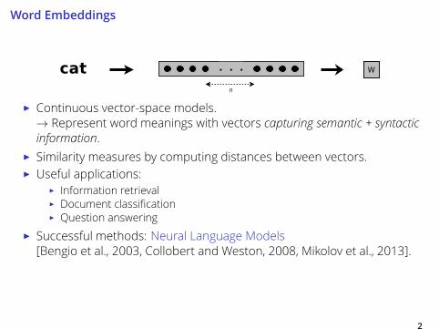
Word Embeddings

I Continuous vector-space models.

→ Represent word meanings with vectors capturing semantic + syntacticinformation.

I Similarity measures by computing distances between vectors.

I Useful applications:

I Information retrieval

I Document classification

I Question answering

I Successful methods: Neural Language Models

[Bengio et al., 2003, Collobert and Weston, 2008, Mikolov et al., 2013].

2

Neural Language Model Understanding

3

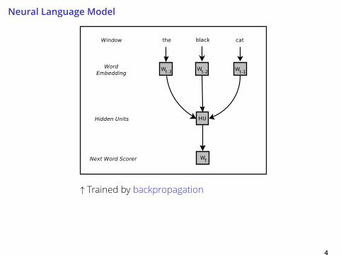
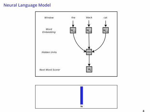
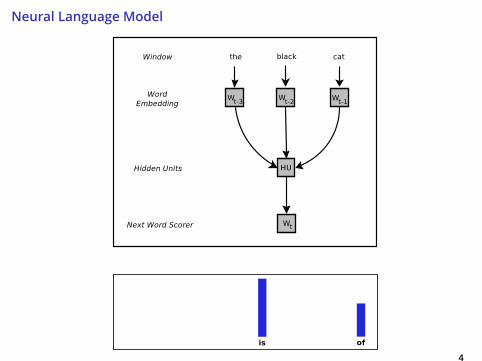
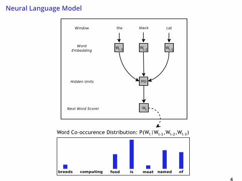
Neural Language Model

4

↑ Trained by backpropagation

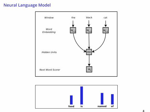
Neural Language Model

4

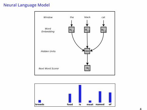
Neural Language Model

4

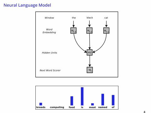
Neural Language Model

4

Neural Language Model

4

Neural Language Model

4

Neural Language Model

4

Use of Context

“You shall know a word by the company it keeps”

[Firth, 1957]

5

Use of Context

5

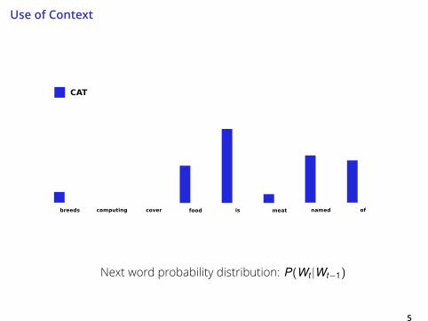
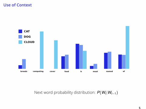
Next word probability distribution: P(Wt |Wt−1)

Use of Context

5

Next word probability distribution: P(Wt |Wt−1)

Use of Context

5

Next word probability distribution: P(Wt |Wt−1)

Neural Language Model

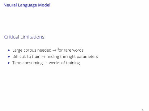
Critical Limitations:

I Large corpus needed→ for rare wordsI Difficult to train→ finding the right parameters

I Time-consuming→ weeks of training

6

Neural Language Model

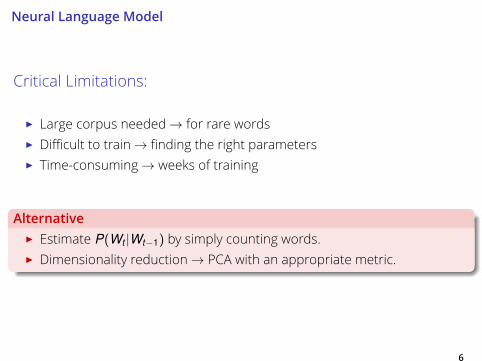
Critical Limitations:

I Large corpus needed→ for rare wordsI Difficult to train→ finding the right parameters

I Time-consuming→ weeks of training

AlternativeI Estimate P(Wt |Wt−1) by simply counting words.

I Dimensionality reduction→ PCA with an appropriate metric.

6

Hellinger PCA of the Word Co-occurence MatrixA simpler and faster method for word embeddings

7

A Spectral Method

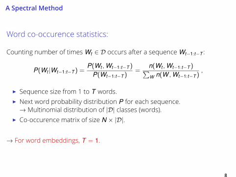
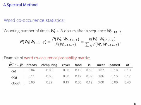
Word co-occurence statistics:

Counting number of timesWt ∈ D occurs after a sequenceWt−1:t−T :

P(Wt |Wt−1:t−T ) =P(Wt ,Wt−1:t−T )

P(Wt−1:t−T )=

n(Wt ,Wt−1:t−T )∑W n(W ,Wt−1:t−T )

,

I Sequence size from 1 to T words.I Next word probability distribution P for each sequence.→ Multinomial distribution of |D| classes (words).

I Co-occurence matrix of size N × |D|.

→ For word embeddings, T = 1.

8

A Spectral Method

Word co-occurence statistics:

Counting number of timesWt ∈ D occurs after a sequenceWt−1:t−T :

P(Wt |Wt−1:t−T ) =P(Wt ,Wt−1:t−T )

P(Wt−1:t−T )=

n(Wt ,Wt−1:t−T )∑W n(W ,Wt−1:t−T )

,

Example of word co-occurence probability matrix:

Wt−1 Wt breeds computing cover food is meat named ofcat 0.04 0.00 0.00 0.13 0.53 0.02 0.18 0.10

dog 0.11 0.00 0.00 0.12 0.39 0.06 0.15 0.17

cloud 0.00 0.29 0.19 0.00 0.12 0.00 0.00 0.40

8

A Spectral Method

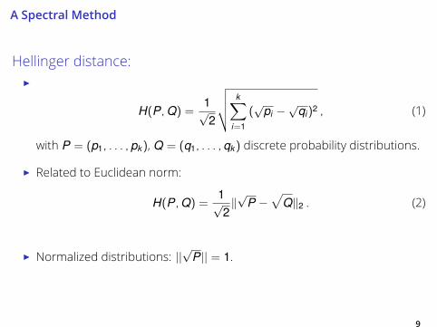
Hellinger distance:

I

H(P,Q) =1√2

√√√√ k∑i=1

(√

pi −√

qi)2 , (1)

with P = (p1, . . . ,pk ), Q = (q1, . . . ,qk ) discrete probability distributions.

I Related to Euclidean norm:

H(P,Q) =1√2‖√

P −√

Q‖2 . (2)

I Normalized distributions: ||√

P|| = 1.

9

A Spectral Method

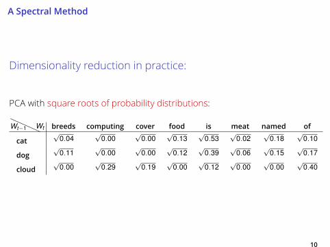
Dimensionality reduction in practice:

PCA with square roots of probability distributions:

Wt−1 Wt breeds computing cover food is meat named ofcat

√0.04

√0.00

√0.00

√0.13

√0.53

√0.02

√0.18

√0.10

dog√

0.11√

0.00√

0.00√

0.12√

0.39√

0.06√

0.15√

0.17

cloud√

0.00√

0.29√

0.19√

0.00√

0.12√

0.00√

0.00√

0.40

10

Word Embeddings Evaluation

11

Word Embeddings Evaluation

Supervised NLP tasks:

I Syntactic: Named Entity RecognitionI Semantic: Movie Review

12

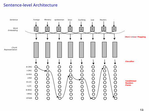
Sentence-level Architecture

13

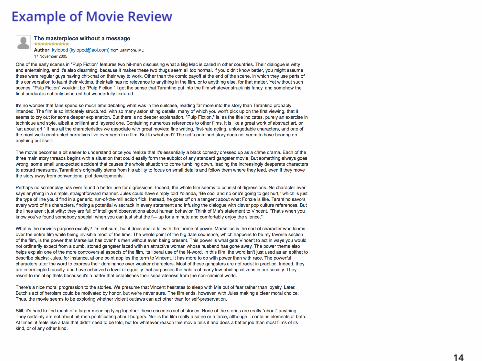
Example of Movie Review

14

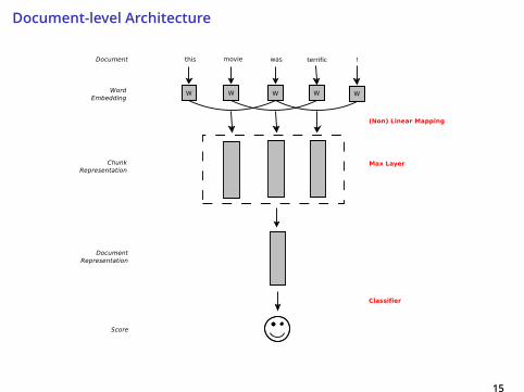
Document-level Architecture

15

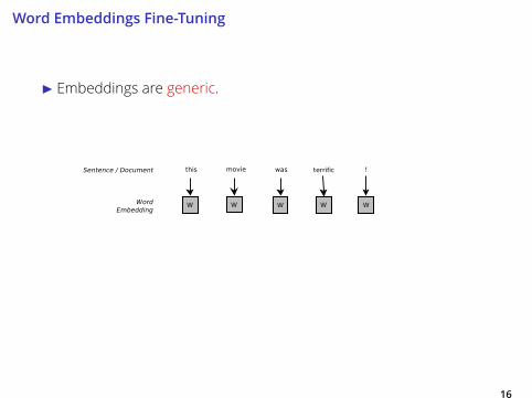
Word Embeddings Fine-Tuning

16

I Embeddings are generic.

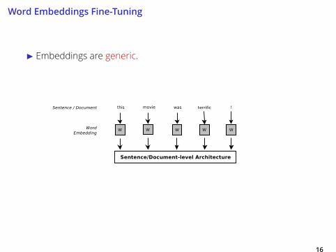
Word Embeddings Fine-Tuning

16

I Embeddings are generic.

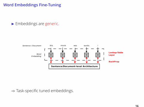
Word Embeddings Fine-Tuning

16

I Embeddings are generic.

⇒ Task-specific tuned embeddings.

Experimental Setup

17

Experimental Setup

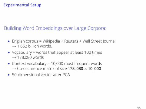
Building Word Embeddings over Large Corpora:

I English corpus = Wikipedia + Reuters + Wall Street Journal

→ 1.652 billion words.I Vocabulary = words that appear at least 100 times

→ 178,080 wordsI Context vocabulary = 10,000 most frequent words

→ Co-occurence matrix of size 178,080× 10,000I 50-dimensional vector after PCA

18

Experimental Setup

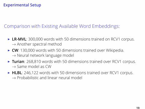
Comparison with Existing Available Word Embeddings:

I LR-MVL: 300,000 words with 50 dimensions trained on RCV1 corpus.→ Another spectral method

I CW: 130,000 words with 50 dimensions trained over Wikipedia.→ Neural network language model

I Turian: 268,810 words with 50 dimensions trained over RCV1 corpus.→ Same model as CW

I HLBL: 246,122 words with 50 dimensions trained over RCV1 corpus.→ Probabilistic and linear neural model

19

Experimental Setup

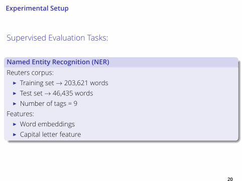
Supervised Evaluation Tasks:

Named Entity Recognition (NER)Reuters corpus:

I Training set→ 203,621 wordsI Test set→ 46,435 wordsI Number of tags = 9

Features:

I Word embeddings

I Capital letter feature

20

Experimental Setup

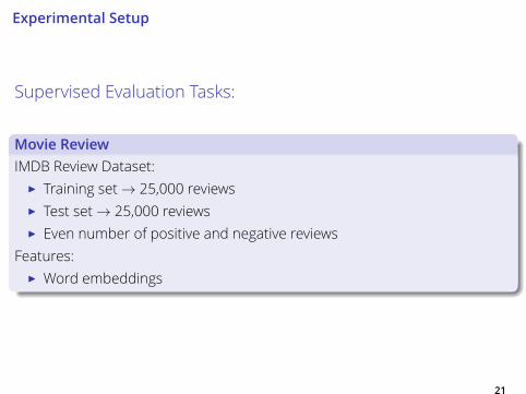
Supervised Evaluation Tasks:

Movie ReviewIMDB Review Dataset:

I Training set→ 25,000 reviewsI Test set→ 25,000 reviewsI Even number of positive and negative reviews

Features:

I Word embeddings

21

Results

22

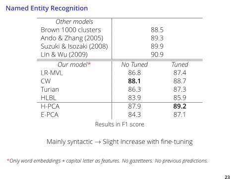
Named Entity RecognitionOther models

Brown 1000 clusters 88.5

Ando & Zhang (2005) 89.3

Suzuki & Isozaki (2008) 89.9

Lin & Wu (2009) 90.9

Our model* No Tuned TunedLR-MVL 86.8 87.4

CW 88.1 88.7

Turian 86.3 87.3

HLBL 83.9 85.9

H-PCA 87.9 89.2E-PCA 84.3 87.1

Results in F1 score

Mainly syntactic→ Slight increase with fine-tuning

*Only word embeddings + capital letter as features. No gazetteers. No previous predictions.

23

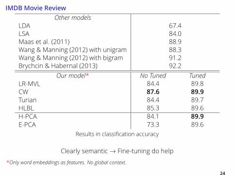
IMDB Movie ReviewOther models

LDA 67.4

LSA 84.0

Maas et al. (2011) 88.9

Wang & Manning (2012) with unigram 88.3

Wang & Manning (2012) with bigram 91.2

Brychcin & Habernal (2013) 92.2

Our model* No Tuned TunedLR-MVL 84.4 89.8

CW 87.6 89.9Turian 84.4 89.7

HLBL 85.3 89.6

H-PCA 84.1 89.9E-PCA 73.3 89.6

Results in classification accuracy

Clearly semantic→ Fine-tuning do help

*Only word embeddings as features. No global context.24

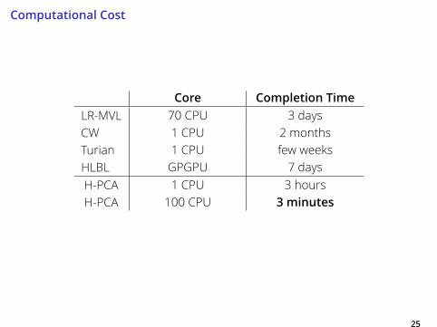
Computational Cost

Core Completion TimeLR-MVL 70 CPU 3 days

CW 1 CPU 2 months

Turian 1 CPU few weeks

HLBL GPGPU 7 days

H-PCA 1 CPU 3 hours

H-PCA 100 CPU 3 minutes

25

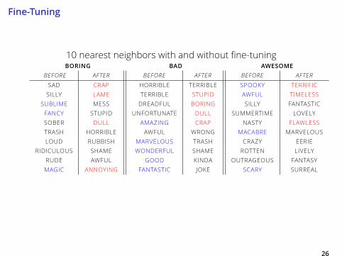
Fine-Tuning

10 nearest neighbors with and without fine-tuning

BORING BAD AWESOMEBEFORE AFTER BEFORE AFTER BEFORE AFTERSAD CRAP HORRIBLE TERRIBLE SPOOKY TERRIFIC

SILLY LAME TERRIBLE STUPID AWFUL TIMELESS

SUBLIME MESS DREADFUL BORING SILLY FANTASTIC

FANCY STUPID UNFORTUNATE DULL SUMMERTIME LOVELY

SOBER DULL AMAZING CRAP NASTY FLAWLESS

TRASH HORRIBLE AWFUL WRONG MACABRE MARVELOUS

LOUD RUBBISH MARVELOUS TRASH CRAZY EERIE

RIDICULOUS SHAME WONDERFUL SHAME ROTTEN LIVELY

RUDE AWFUL GOOD KINDA OUTRAGEOUS FANTASY

MAGIC ANNOYING FANTASTIC JOKE SCARY SURREAL

26

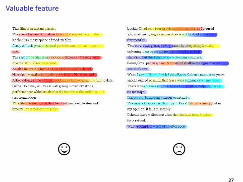
Valuable feature

© §

27

Conclusion

I Appealing word embeddings from Hellinger PCA of the wordco-occurence matrix.

→ Simply counting words over a large corpus.

I PCA of a N × 10,000matrix→ fast and not memory consuming.→ Practical alternative to neural language models.

I H-PCA’s embeddings available online:

→ 50, 100 and 200 dimensions→ Demo→ http://www.lebret.ch/words

Thank you !

28

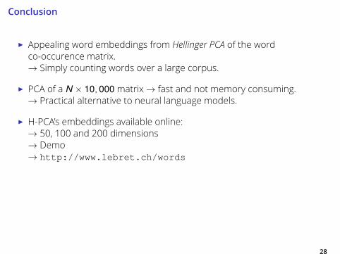
Conclusion

I Appealing word embeddings from Hellinger PCA of the wordco-occurence matrix.

→ Simply counting words over a large corpus.

I PCA of a N × 10,000matrix→ fast and not memory consuming.→ Practical alternative to neural language models.

I H-PCA’s embeddings available online:

→ 50, 100 and 200 dimensions→ Demo→ http://www.lebret.ch/words

Thank you !

28

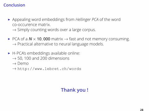
References I

Bengio, Y., Ducharme, R., Vincent, P., and Janvin, C. (2003).

A neural probabilistic language model.

J. Mach. Learn. Res., 3:1137–1155.Collobert, R. and Weston, J. (2008).

A unified architecture for natural language processing: Deep neural networks

with multitask learning.

In International Conference on Machine Learning, ICML.Collobert, R., Weston, J., Bottou, L., Karlen, M., Kavukcuoglu, K., and Kuksa, P.

(2011).

Natural language processing (almost) from scratch.

Journal of Machine Learning Research, 12:2493–2537.Firth, J. R. (1957).

A synopsis of linguistic theory 1930-55.

1952-59:1–32.

29

References II

Mikolov, T., Sutskever, I., Chen, K., Corrado, G., and Dean, J. (2013).

Distributed representations of words and phrases and their compositionality.

In Burges, C., Bottou, L., Welling, M., Ghahramani, Z., and Weinberger, K., editors,

Advances in Neural Information Processing Systems 26, pages 3111–3119. CurranAssociates, Inc.

30

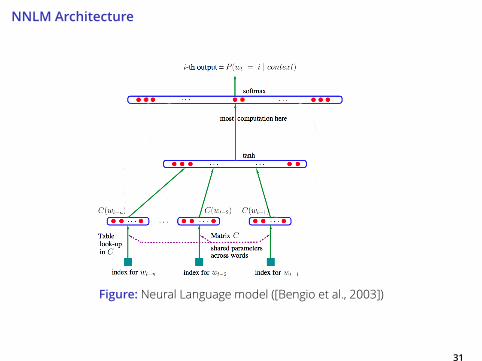
NNLM Architecture

Figure: Neural Language model ([Bengio et al., 2003])

31

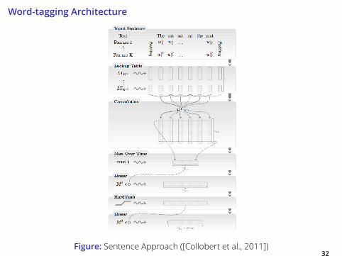
Word-tagging Architecture

Figure: Sentence Approach ([Collobert et al., 2011])32