CEREAL MARKET PERFORMANCE IN ETHIOPIAdocuments.worldbank.org/curated/en/... · CEREAL MARKET PERFORMANCE IN ETHIOPIA: Policy Implications for Improving Investments in Maize and Wheat

CEREAL MARKET PERFORMANCE IN ETHIOPIA:

Policy Implications for Improving Investments in Maize and Wheat Value Chains

May 30, 2018

Agriculture Global Practice GFA13

Pub

lic D

iscl

osur

e A

utho

rized

Pub

lic D

iscl

osur

e A

utho

rized

Pub

lic D

iscl

osur

e A

utho

rized

Pub

lic D

iscl

osur

e A

utho

rized

1

Table of Contents

Acronyms and Abbreviations ................................................................................................................. 3

List of Figures ........................................................................................................................................ 6

List of Tables ......................................................................................................................................... 6

Executive Summary ............................................................................................................................... 8

I. Background and Justification ........................................................................................................ 8

II. Methodology and Data .................................................................................................................. 9

III. Main Findings ............................................................................................................................... 10

1. Introduction .................................................................................................................................. 18

2. The Maize and Wheat Sub-sectors .............................................................................................. 20

2.1. The Role of maize and wheat in Ethiopia ....................................................................................... 20

2.2. The maize and wheat value chains ..................................................................................................................... 22

2.2.1. Production of maize and wheat .................................................................................................................. 22

2.2.2 Grain storage ......................................................................................................................................... 23

2.2.3. Maize and wheat marketing ................................................................................................................. 24

Figure 1: Wheat Value Chain Map ...................................................................................................... 25

Figure 2: Maize Value Chain Map ...................................................................................................... 26

3. Conceptual Framework and Empirical Strategy.......................................................................... 33

3.1 A conceptual framework for cereal market performance analysis ................................................ 33

3.2. Measuring the levels and variability of maize and wheat prices .................................................... 35

3.2.1 Analyzing maize and wheat price levels and variability .................................................................. 35

3.2.1.1 Overall maize and wheat price fluctuations ...................................................................................... 35

3.2.1.2 Measuring seasonal price movements and temporal arbitrage opportunities ............................ 36

3.2.1.3 Measuring the volatilities of maize and wheat prices........................................................................ 40

3.2.1.4. Measuring maize and wheat markets integration: A spatial price analysis .................................. 42

4. Data sources and limitations ....................................................................................................... 46

4.1 Sources of data ...................................................................................................................................... 46

4.2 Data limitations .................................................................................................................................... 47

5. Empirical results on the performance of maize and wheat markets ........................................... 48

5.1 Trends in maize and wheat price levels ............................................................................................. 48

5.2 Fluctuations in maize and wheat prices ............................................................................................. 50

5.2.1. Results of variance decomposition ................................................................................................... 50

5.2.2. Time series decomposition of maize and wheat prices .................................................................. 52

5.2.3. Descriptive statistics of monthly price changes and returns for maize and wheat crops ................. 56

5.2.4. How volatile are maize and wheat prices? ................................................................................................. 61

2

5.3. The relationship between producer and wholesale prices .............................................................. 64

5.3.1. Descriptive analysis of maize and wheat wholesale price margins ............................................... 64

5.4. Are maize and wheat markets integrated?......................................................................................... 65

5.4.1. Descriptive analysis of maize and wheat spatial differentials ........................................................ 65

5.4.2. Econometric tests results..................................................................................................................... 68

5.4.2.1. Unit root tests ........................................................................................................................................ 68

5.4.2.2. Long-run spatial equilibrium relationship in maize markets .......................................................... 69

5.4.2.3. The short-run dynamic relationship between selected wholesale maize markets ....................... 71

5.4.2.4. The long-run spatial equilibrium relationship in wheat markets ................................................... 73

5.4.2.5. The short-run dynamic relationship between selected wholesale wheat markets ....................... 73

6. Conclusions and policy implications ................................................................................................................... 77

6.1 Conclusions............................................................................................................................................ 77

6.2 Policy implications ................................................................................................................................ 78

Implications for policy options and actions ............................................................................................................. 78

References ........................................................................................................................................................................ 82

Annex 1: Evolution of nominal and real maize prices (December 2011=100) for selected markets in Ethiopia,

2001 to 2017……………………………………………………………………………………………….85

Annex 2: Evolution of nominal and real wheat prices (December 2011=100) for selected markets in

Ethiopia, 2001 to 2017………………………………………………………………………….………… 86

Annex 3: Historical volatiltity of real producer maize prices, Ethiopia 2001-2016…….…………..……… 87

Annex 4: Historical volatiltity of real producer wheat prices, Ethiopia 2001-2016………………………… 88

3

Acknowledgements

This report was prepared by a team including: Hikuepi B. Katjiuongua, Task Team Leader and Senior

Agricultural Economist, Global Food Agriculture Practice (GFA), Asfaw Muleta, Consultant GFA and John

Nash, Consultant GFA. The task team is grateful for excellent input at the conceptualization stage of this

study provided by Andrew Goodland, Program Leader, SACSL, and Sarah Coll-Black, Senior Social

Protection Specialist. The team is also grateful to Manex Bole Yonis, World Bank Consultant, and Mekdim

Dereje for their excellent input related to data collection and input during fieldwork.

Overall guidance was provided by Mark Cackler, Practice Manager, GFA13. The following peer reviewers

provided excellent feedback at different stages of the study: Samuel Taffesse, Senior Agriculture Economist,

GFAGE; Holger Kray, Lead Agriculture Economist, GFA13; Blessings Botha, Agricultural Economist,

GFA13; Panos Varangis, Head, GFCLT – IFC, and Ijeoma Emenanjo, Sr Agricultural Specialist, GFA13.

The team also benefitted from both written and verbal comments provided by many individuals, including

Richard Spencer, Program Leader, AFCE3; Vikas Choudhary, Senior Agricultural Specialist, GFA13; Lucian

Bucur Pop, Sr Social Protection Specialist, GSP01; Abu Yadetta Hateu, Sr Social Protection Specialist, GSP01

and anonymous reviewers. In addition, Assaye Legesse, Senior Agricultural Economist, GFA, Teklu Toli,

Senior Agricultural Specialist, GFA and Welela Ketema, Sr Agricultural Specialist, GFA, provided great

support during the study results validation workshop. The task team benefited from excellent administrative

support at various stages from Adiam Berhane, Team Assistant (AFCE3), Azeb Afework, Program Assistant

(AFCE3) and Tesfahiwot Dillnessa, Program Assistant (GSU07).

The team is grateful to various Government institutions and agencies that provided data, information and

consultations including: Ministry of Finance and Economic Cooperation, Ministry of Agriculture and

Livestock Resources, Ministry of Trade and Industry; Ethiopian Trading Business Corporation; Central

Statistics Agency, Agricultural Transformation Agency, Federal Cooperative Agency and Cooperative

Agencies at regional level, Ethiopian Commodity Exchange, and private sector key informants including

farmers, traders and millers.

We gratefully acknowledge generous financial support from the Agricultural Growth Project and various

Trust Funds of the Second Agricultural Growth Project and the Productive Safety Net Project 4.

4

Acronyms and Abbreviations

ATA Agricultural Transformation Agency

ADF Augmented Dickey-Full

AGP Agricultural Growth Project

AGP2 Second Agriculture Growth Project

AIC Akaike information criterion

AMC Agricultural Marketing Corporation

ANOVA Analysis of Variance

ARCH Autoregressive Heteroscedasticity

CSA Central Statistics Agency

ECX Ethiopian Commodity Exchange

ECM Error Correction Model

EDRI Ethiopia Development Research Institute

EFSRA Ethiopian Emergency Food Security Reserve Administration

EGTE Ethiopian Grain Trade Enterprise

ETB Ethiopian Birr

ETBC Ethiopian Trading Business Corporation

ECX Ethiopian Commodity Exchange

FCA Federal Cooperative Agency

FGD Focus group discussions

GARCH Generalized Autoregressive Heteroscedasticity

GoE Government of Ethiopia

GSR Gross storage return

HL Half-Life

IDA International Development Association

IFPRI International Food Policy Research Institute

JEOP Joint Emergency Operations Partners

LB Lijung-Box

LM Lagrange Multiplier

NDRMC National Disaster Risk Management Commission

OLS Ordinary least squares

PAC Partial autocorrelation

PBM Parity Bound Modeling

PP Philipps-Perron

5

PSNP Productive Safety Net Program

SBIC Schwarz’s Bayesian Information Criterion

SNNP Southern Nations and Nationalities People

TAR Threshold Auto Regressive

TVECM Threshold Vector Error Correction Model

USAID United States Agency for International Development

VC Value Chain

WFP World Food Program

6

List of Figures

Figure 1: Wheat value chain map .................................................................................................................................. 25 Figure 2: Maize value chain map ................................................................................................................................... 26

List of Tables

Table 1: Summary Statistics of Monthly Real Producer Prices for Maize in Selected Markets in Ethiopia,

(Birr/100kg, 2002-2016) ................................................................................................................................... 48 Table 2: Summary Statistics of Monthly Real Wholesale Prices of Maize in Selected Markets in Ethiopia, ..... 48 Table 3: Summary Statistics of Monthly Real Retail Prices of Maize in Selected Markets in Ethiopia,

(Birr/100kg, 2002-2016) ................................................................................................................................... 49 Table 4: Summary Statistics of Monthly Real Producer Prices for Wheat in Selected Markets in Ethiopia,

(Birr/100kg, 2000-2016) ................................................................................................................................... 49 Table 5: Summary Statistics of Monthly Real Wholesale Prices for Wheat in Selected Markets in Ethiopia,

(Birr/100kg, 2002-2016) ................................................................................................................................... 49 Table 6: Summary Statistics of Monthly Real Retail Prices for Wheat in Selected Markets in Ethiopia,

(Birr/100kg, 2002-2016) ................................................................................................................................... 50 Table 7: Variance Decomposition of Fluctuations in Real Prices of Maize in Selected Markets in Ethiopia,

2002-2016 ............................................................................................................................................................ 51 Table 8: Variance Decomposition of Fluctuations in Real Prices of Wheat in Selected Markets in Ethiopia,

2002-2016 ............................................................................................................................................................ 52 Table 9: Grand Seasonal Producer Price Indices for Maize in Selected Markets in Ethiopia, 2002-2016 ......... 53 Table 10: Grand Seasonal Wholesale Price Indices for Maize in Selected Markets in Ethiopia, 2002-2016 ..... 53 Table 11: Grand Seasonal Retail Price Indexes for Maize in Selected Markets in Ethiopia, 2002-2016 ............ 54 Table 12: Grand Seasonal Producer Price Indices for Wheat in Selected Markets in Ethiopia, 2002-2016 ...... 55 Table 13: Grand Seasonal Wholesale Price Indices for Wheat in Selected Markets in Ethiopia, 2002-2016 .... 55 Table 14: Grand Seasonal Retail Price Indices for Wheat in Selected Markets in Ethiopia, 2002-2016 ............ 56 Table 15: Summary Statistics of Monthly Nominal Producer Price Changes for Maize in Selected Markets in

Ethiopia, (Birr/100 kg, 2002-2016) ................................................................................................................. 57 Table 16: Summary Statistics of Monthly Nominal Wholesale Price Changes for Maize in Selected Markets in

Ethiopia, Birr/100 kg, 2002-2016 ................................................................................................................... 57 Table 17: Summary Statistics of Monthly Nominal Producer Price Changes for Wheat in Selected Markets in

Ethiopia, (Birr/100 kg, 2002-2016) ................................................................................................................. 58 Table 18: Summary Statistics of Monthly Nominal Wholesale Price Changes for Wheat in Selected Markets in

Ethiopia, (Birr/100 kg, 2002-2016) ................................................................................................................. 58 Table 19: Summary Statistics of Monthly Real Producer Price Returns: Percentage for Maize in Selected

Markets in Ethiopia, 2002-2016 ...................................................................................................................... 58 Table 20: Summary Statistics of Monthly Real Wholesale Price Returns: Percentage for Maize in Selected

Markets in Ethiopia, 2002-2016 ...................................................................................................................... 59 Table 21: Summary Statistics of Monthly Real Retail Price Returns: Percentage for Maize in Selected Markets

in Ethiopia, 2002-2016 ...................................................................................................................................... 59 Table 22: Summary Statistics of Monthly Wheat Producer Price Returns: Percentage of Wheat in Selected

Markets in Ethiopia, 2002-2016 ...................................................................................................................... 59 Table 23: Summary Statistics of Monthly Real Wholesale Price Returns: Percentage of Wheat in Selected

Markets in Ethiopia, 2002-2016 ...................................................................................................................... 60

7

Table 24: Summary Statistics of Monthly Real Retail Price Returns: Percentage of Wheat in Selected Markets

in Ethiopia, 2002-2016 ...................................................................................................................................... 60 Table 25: Summary Statistics of Unconditional Volatilities of Real Producer Prices of Maize in Selected

Markets in Ethiopia, 2002-2016 ...................................................................................................................... 61 Table 26: Summary Statistics of Unconditional Volatilities of Real Wholesale Prices of Maize in Selected

Markets in Ethiopia, 2002-2016 ...................................................................................................................... 62 Table 27: Summary Statistics of Unconditional Volatilities of Real Retail Prices of Maize in Selected Markets

in Ethiopia, 2002-2016 ...................................................................................................................................... 62 Table 28: Summary Statistics of Unconditional Volatilities of Real Producer Prices of Wheat in Selected

Markets in Ethiopia, 2002-2016 ...................................................................................................................... 62 Table 29: Summary Statistics of Unconditional Volatilities of Real Wholesale Prices of Wheat in Selected

Markets in Ethiopia, 2002-2016 ...................................................................................................................... 63 Table 30: Summary Statistics of Unconditional Volatilities of Real Retail Prices of Wheat in Selected Markets

in Ethiopia, 2002-2016 ...................................................................................................................................... 63 Table 31: Results of GARCH Parameter Estimates of Monthly Real Producer and Wholesale Maize Prices for

Selected Markets in Ethiopia, 2002-2016 ....................................................................................................... 63 Table 32: Results of GARCH Parameter Estimates of Monthly Real Producer and Wholesale Wheat Prices

for Selected Markets in Ethiopia, 2002-2016 ................................................................................................ 64 Table 33: Summary Statistics of Nominal Wholesale Price Margins for Maize in Selected Markets in Ethiopia,

(Birr/100 kg, 2002-2016) .................................................................................................................................. 65 Table 34: Summary Statistics of Monthly Nominal Wholesale Price Margins for Wheat in Selected Markets in

Ethiopia, (Birr/100 kg, 2002-2016) ................................................................................................................. 65 Table 35: Summary Statistics of Monthly Spatial Real Price Differentials for Maize in Selected Maize Market

Pairs in Ethiopia, (prices deflated by consumer price index (CPI) (Dec 2011=100), 2002- 2016) ...... 66 Table 36: Summary Statistics of Monthly Inter-regional Price Returns to Maize Trade between Selected

Markets in Ethiopia, (price deflated by CPI (Dec 2011=100), 2002-2016 ............................................... 66 Table 37: Summary Statistics of Monthly Nominal Spatial Wheat Price Differentials for Selected Market Pairs

in Ethiopia, (prices deflated by CPI (Dec 2011=100), 2002-2016) ........................................................... 67 Table 38: Summary Statistics of Annualized Inter-regional Price Returns to Wheat Trade between Selected

Markets in Ethiopia, (price deflated by CPI (Dec 2011=100), 2002-2016 ............................................... 68 Table 39: The Results of Tests for the Long-run Equilibrium Relationship between Selected Wholesale Maize

Market Pairs in Ethiopia, 2002-2016 .............................................................................................................. 69 Table 40: The Results of Threshold Co-integration Tests for Selected Maize Wholesale Market Pairs in

Ethiopia, 2002-2016 .......................................................................................................................................... 70 Table 41: Short-run Dynamic Relationships between Selected Wholesale Maize Markets in Ethiopia,

2002-2016 ............................................................................................................................................................ 72 Table 42: Results of the Tests for Long-run Equilibrium Relationships between Selected Wholesale Wheat

Market Pairs in Ethiopia, 2002-2016 .............................................................................................................. 74 Table 43: The Results of Threshold Co-integration Tests for Selected Wheat Wholesale Market Pairs in

Ethiopia, 2002-2016 .......................................................................................................................................... 75 Table 44: Short-run dynamic relationships between selected wholesale wheat markets in Ethiopia,

2002-2016 ............................................................................................................................................................ 75

8

Executive Summary

I. Background and Justification

The efficient functioning of cereal markets is important given the significant share of cereals in food

expenditures of households in low-income countries. Cereals comprise half of consumer food

expenditures in Ethiopia, and about 75 percent of the land area under cultivation (Central Statistics

Agency 2012). With the recent food price inflation and concerns regarding the impact of the 2015/26

drought related to El Nino, understanding the performance of food markets has found renewed

interest among governments, development banks, and local and international organizations.

For Ethiopia, this is particularly relevant given the disastrous implications that poorly functioning food

markets have had in the past on food security (Minten et al, 2014). Due to these concerns, price

stabilization and food security have emerged as the two key objectives behind the government’s policy

on grain marketing. To stabilize grain prices and reduce the risk of high price volatility in the food

sector, the government maintains a strategic stock reserve, and has banned grain exports in response

to rising prices (2006-2008). In the case of wheat, it imports wheat and sells it at subsidized prices to

selected mills that eventually sell to retailers at a fixed price. The retailers then sell the subsidized bread

to consumers. In addition, relief agencies provide food aid to assist food insecure households. The

Productive Safety Nets Program (PSNP) also assists through cash and food transfers.

How well cereal markets are integrated across time and space matters. This has implications for the

efficiency of cereal markets and the effectiveness with which they can respond to food emergencies

in the country. Further, post-harvest handling and storage investments are critical to ensuring the

availability of grains, especially in enabling the government to respond to food emergencies. However,

the level of price volatility affects marketing and storage decisions at all levels of the value chain.

Volatile food prices would also affect the procurement decisions of agri-businesses involved in food

distribution, processing, and retailing such that farmers would be faced with lower and more variable

demand in selling markets. The aggregate effect is reduced economic activity in the food sector. This

leads to a decreased and variable supply of food commodities and food products, which in turn further

exacerbates price volatility. It also generates upward pressure on food prices for consumers (World

Bank 2016). Hence, assessing the performance of cereal markets requires in-depth analysis regarding

price volatility as it is a good indicator of the level of risk in the market, which in turn affects the

behavior of the value chain actors.

Currently, there is little private sector investment in grain storage facilities. Most storage warehouses

at the primary cooperative and farmers’ union levels are funded by the public sector. About $32.7

million of International Development Association (IDA) funds under the Agriculture Growth Project

(AGP) were allocated for market infrastructure development, including piloting the construction of

forty-four storage warehouses with the objective of further scaling up. Under AGP 2, the government

requested $11 million toward the construction of more storage warehouses for unions and primary

cooperatives.

9

Before constructing more warehouses, though, it is important to shed light on why the private sector

is not investing in grain storage. Is public sector investment in grain storage facilities crowding out

private investment or are the incentives for the private sector to invest in storage low and, if so, why?

Although the government regards cooperatives as private entities, public resources subsidize most of

their marketing infrastructure investments.

The objective of this study is to provide an updated overview about the performance of cereal markets.

Specifically, it aims to inform and guide project operations for the Government of Ethiopia (GoE)

and the World Bank. First, it seeks to inform the government about incentives regarding grain storage

before it makes more public investments in such facilities at the cooperative and union levels. Second,

both the GoE and the World Bank need a better understanding about the performance of cereal

markets, including the constraints on private sector investment in storage facilities. Further, to respond

to increasing demand from the government for more food-based (non-market) interventions to

provide access to food to the poor (instead of market-based (cash or voucher transfers) interventions),

the PSNP program will need to be better informed about the level and extent of cereal market

integration. Finally, the results from this study will also inform proposed IFC operations pertaining

to the Ethiopia Commodity Collateralized Financing (CCF) project.

Wheat and maize are the most important cereals in Ethiopia. Maize provides the highest share of

caloric intake for consumers, accounting for 17-20 percent of the total (Abate and others 2015; United

States Agency for International Development [USAID], 2017). It is particularly important for poor

households, as they mix maize flour with teff to make the national staple injera and the cost of maize

is half that of wheat and teff. Maize represents 30 percent of total cereal production, with

approximately 17 percent of the total cereal area characterized by a low level of productivity. As part

of the government’s policy to stabilize staple food prices for food security, the exporting of maize is

banned. Wheat and wheat products represent 14 percent of total caloric intake for consumers. Unlike

maize, demand for wheat increases as incomes rise, and the demand for wheat has grown significantly

over the last decade. It is imported in large volumes (approximately 1.8 million MT per year). Indeed,

the government has continuously imported wheat for the last several years and distributed it to

contracted large millers to sell flour. It is argued that subsidized wheat has been creating disincentives

related to domestic wheat marketing and production.

Thus, given the significant importance of maize and wheat, the analysis in this study focuses on these

two commodities. Although some of the analysis and results provide insights on the general marketing

conditions for other important cereals such as teff and sorghum, more time and resources are needed

to extend the price analysis to these other cereals.

II. Methodology and Data

The research method combines market-level temporal and spatial price analysis with a detailed analysis

at the producer, wholesale and retail levels for maize and wheat value chains. The goal is to shed light

on market performance, and to identify factors affecting the capacity of value chain (VC) actors to

10

expand and invest in grain marketing opportunities. Some of the key features modeled include: (1)

maize and wheat price volatilities to gauge the level of risk in their respective markets; (2) seasonal

price movements to assess the level of temporal arbitrage opportunities and efficiencies; and (3) spatial

price linkages to assess the level of spatial arbitrage opportunities, efficiencies and market integration.

The spatial price analysis models were considered at the different stages, but the key questions they

answer relate to the elasticity of price transmission between different markets and/or stages of

marketing, and the size and the persistence of price shocks. Seasonal patterns of cereal prices were

analyzed using seasonal decomposition methods. The method decomposed the time-series price data

into four components: the seasonal, the random component, and the trend and cyclical components.

The aim is to isolate and develop seasonal price indices (for both wheat and maize), which are

important in storage decisions, as well as to shed light on the potential for temporal arbitrage.

The study is based on a review of literature, a rapid appraisal of maize and wheat production and

marketing systems, and statistical and econometric analyses of time-series price data obtained from

secondary sources. The time-series monthly nominal prices of maize and wheat were collected at

different market levels (producer, wholesale and retail) for selected markets from both grain surplus

producing and grain deficit regions. The wholesale price data for maize and wheat is reported in

Ethiopian Birr per quintal (100 kilograms) and is obtained from the Ethiopian Trade and Business

Corporation (ETBC1).

III. Main Findings

Maize and wheat markets are integrated in the long run, but price transmission is incomplete

and asymmetric. The econometric results indicate that there is a long-run relationship between

spatially separated maize and wheat markets. This is indicative of the improvements in road

infrastructure, and the availability of trucks and mobile communications. However, the long-run price

transmission between the deficient and surplus markets is less than complete, and the adjustments to

price changes in different markets are asymmetric. A higher level of long-run price transmission is

observed for maize. However, the long-run elasticity of price transmission is less than 50 percent in

seven of the 21 wheat markets considered. This could be due to asymmetric market information,

transaction costs, and government interventions. Overall, the results point to a need to provide, among

other things, regular market intelligence and analytical support to the value chain actors.

There is a significant degree of unpredictability in wheat and maize prices, implying a high

risk for the value chain actors. The results show that there has been a slight upward movement in

nominal and real prices of maize and wheat in different markets and at all market levels (producer,

wholesale and retail). However, there is significant unpredictability in maize and wheat prices, thus

making spot market temporal and spatial arbitrage a risky business for value chain actors. For example,

in the case of maize markets, about 6 to 33 percent (at the producer level), 0 to 72 percent (at the

1 Formerly known as the Ethiopian Grain Trade Enterprise (EGTE) for the period from January 2001 to December 2016.

11

wholesale level) and 2 to 45 percent (at the retail level) of the overall maize price fluctuations are

explained by unpredictable random price movements. The corresponding figures in the case of wheat

are 0 to 27 percent (at the producer level), 1 to 27 percent (at the wholesale level) and 0 to 46 (at the

retail level).

The consequence of increased volatility would be limited maize and wheat market transactions as

market actors avoid risks. This also decreases the availability of maize and wheat both temporally and

spatially. Furthermore, given the non-existence of efficient mechanisms for price risk management,

such as a futures market, high risks would discourage necessary investments in maize and wheat

production, marketing, distribution and logistics — which are all necessary to increasing the

competitiveness of the maize and wheat value chains. This presents significant bottlenecks to the

government’s agricultural transformation agenda, which seeks to improve smallholder’s adoption of

modern agricultural inputs and increase their commercialization.

To address the risk of high price volatility would require changes at the policy level related to grain

procurement and distribution, and investments in the institutions and infrastructure which would

increase the transparency and stability of the maize and marketing systems. For example, investments

could be made in agricultural market information systems, a strengthening of food safety and quality

standards and grades, and development of a commodity exchange.

Although there is significant seasonality in maize and wheat prices, the returns are low with

high volatility. There is significant seasonality for maize and wheat prices in different markets and at

different value chain nodes. However, the implied storage periods for wheat and maize required

between the seasonal low and high prices appear to be very long (5 to 10 months). The empirical

results indicate that holding wheat and maize stock for such a lengthy period does not provide

sufficient incentives, given the very low but highly volatile monthly price returns for maize and wheat

stocks. The analysis shows excessive downward and upward movements in actual maize and wheat

prices and returns at the producer and wholesale levels, which cannot be explained by the costs of

storage alone. The field observations also indicate limited commercial maize and wheat storage at the

wholesale level, which could be due to the perceived risk of very high price volatility. Overall, there

are limited temporal arbitrage (storage) opportunities in the maize and wheat markets for producers

and wholesalers.

With such high unpredictability and volatility in maize and wheat prices, it is risky for the

private sector to invest in storage. The results imply low commercial incentives to invest in wheat

and maize storage. This may partially explain the current low level of investment by the private sector

in storage facilities. However, given the observed need for good quality storage to minimize post-

harvest losses, the results imply that there is a role for the public sector in making investments in

storage, but it is critical to debate how, at what level, and under what conditions such investments

should be made. The government is currently making these investments at the cooperative level, but

very little grain is sold through cooperatives. Thousands of individual farmers are members of primary

12

cooperatives. This indicates that cooperatives are a useful organizational platform. In this regard,

interventions related to effective and professional management are required to achieve effective staple

food bulking and marketing through cooperatives. Further, results imply an urgent need to address

various issues to improve transparency related to stock and price information, as well as grain

marketing policy.

At the wholesale level, returns to maize and wheat aggregation (wholesale-to-produce price

margin) are better than holding grain. For grain traders, the monthly returns from holding maize

or wheat stock and the regional wholesale traders’ margin2 and the inter-regional grain trader’s margin3

indicate that grain traders in the surplus markets are more interested in buying grain from the farmers

and selling it quickly to the inter-regional wholesale traders. The monthly spatial differential is higher

than the monthly return on holding maize and wheat stock.

There are high levels of post-harvest losses and most farmers sell most of their marketable

grain right after the harvest. Most farmers sell immediately after the harvest to meet different

financial obligations, which are usually due right after the harvest. They also seek to minimize post-

harvest losses, which are approximately more than 10 percent for maize and wheat. In areas where

microfinance service providers are available, the timing of the loan provision is not designed in a way

to prevent the farmers from selling their crops after harvest and debt collection. Furthermore,

producers mostly sell to the traders on credit in advance of harvest time, with the agreement to pay in

kind at cheap rates immediately after harvest when the price is the lowest of the season. Consequently,

most producers do not benefit from better prices because of untimely sales and weak bargaining

power. Although paradoxical, given the observed storage losses combined with results from temporal

and spatial price analyses showing high volatility and unpredictability, and incomplete and asymmetric

price adjustments, it seems that famers may currently be better off selling at harvest time rather than

waiting for higher prices.

Producers sell a negligible amount of grain through primary cooperatives. Field data and

information show that producers sell only a small fraction of their output through cooperatives. The

2016 AGP 2 baseline survey4 of 10,924 randomly selected households reveals that farmers only sell

2.6 percent of their crops through cooperatives. The data further reveal that households sell 1.9

percent (wheat) and 3.8 percent (maize) of their output through cooperatives, whereas 66 percent

(wheat) and 64 percent (maize) is sold through private traders. There are several reasons why so little

grain is marketed through cooperatives by producers, including: (1)cooperatives buy immediately after

2 The difference between the wholesale and producer prices in a market. 3 The price difference between deficit and surplus grain market wholesale prices. 4 Agricultural Growth Project (AGP) II Baseline Draft Survey Report (EDRI, 2017). The data covers four regions including high-surplus grain areas.

13

harvest during a short window of time when prices are low; (2) many producers view the cooperatives as an

unreliable marketing outlet for the farmers in terms of the amount they purchase, their consistency in

purchasing, the length of purchase and the price they offer; (3) most primary cooperatives have

financial constraints and poor market linkages to purchase the desired quantity from their members,

thereby making their purchasing pattern and quantities limited and unpredictable; and (4) other buyers

such as traders pay immediately upon purchase

Storage warehouses, especially at the producer and trader levels, are of low quality and

capacity. Producers, cooperatives, traders and wholesalers noted that there is a shortage of storage,

especially modern storage facilities. One reason cited by farmers for selling a large proportion of their

grain right after the harvest is to minimize post- harvest losses due to lack of proper storage facilities.

In addition, losses during storage due to weevils, rodents and fungus discourage farmers from storing

grain for long periods of time. Some cooperative unions are not able to buy all the grain from the

cooperatives due to limited storage and working capital, which creates problems with primary

cooperatives and their members. As a result, primary cooperatives sometimes sell grain at reduced

prices to the unions due to limited cooperative storage. However, through field observations and

interviews, it was found that most cooperatives primarily store inputs, such as fertilizers and seeds, to

distribute to farmers. Furthermore, most of the existing one-structured storage facilities do not meet

the multi-purpose storage needs at the farm, cooperative and union levels. Ideally, what the farmers

want is separate storage facilities for grains, fertilizers and improved seeds. Currently, due to the shortage of

proper storage facilities, the farmers use the same facility to store farm inputs and outputs

simultaneously or alternatively. This creates potential food safety and health problems, as well as

logistical issues due to small storage capacity.

There is a lack of coordination and planning among grain importing entities, leading to sub-

optimal utilization of the existing public storage system. The lack of coordination and planning

among the key entities involved in importation, including the ETBC — and among the Joint

Emergency Operations Partners (JEOP), the World Food Program (WFP) and the National Disaster

Risk Management Commission (NDRMC) — results in little swapping of warehouses within the

public storage system. Consequently, at times, some public storage warehouses would be empty for

months, while others are overfilled and not able to store any more grain. Each entity imports grains

for their own program, with little synchronization with other importers. This sometimes results in

large grain shipments arriving at the same time at the port in Djibouti, leading to congestion and delays

in shipment deliveries. In this context, the simultaneous arrival of imported wheat in the country

affects local prices.

Maize and wheat transactions are primarily volume-based; there are no market incentives to

ensure the quality of the grain due to lack of regulations on quality and standards. Although

14

many buyers assign grades, there are no formal maize and wheat grain standards. Furthermore, there

are no formal and consistent quality enforcement mechanisms at the different nodes in either value

chain. The grain is examined physically for breakage and obvious physical impurities. There are no

quality checks for moisture content or to store the grain at the appropriate moisture and temperature

levels. Indeed, many cooperatives do not provide important preconditioning services, such as sorting,

drying, and grading before storing the grain. Traders handle low-quality wheat and mix wheat of

different quality, thereby reducing the average quality of wheat flowing through the value chain.

Farmers in Ethiopia can produce good quality bread, pasta wheat, and maize for maize flour, but the

weak market linkages and the lack of quality enforcement do not encourage farmers to invest more in

quality. The lack of third-party inspection of quality standards and grades — and different weighing

scales used by various VC actors — contributes to mistrust and cheating in the cereal marketing

system.

There is a lack of transparency on price discovery, and asymmetric cereal price information

contributes to uncertainties in the marketing system. Many actors in the maize and wheat value

chain reveal that there is a lack of transparency regarding how wheat and maize prices are determined.

Prices are not announced to the grain value chain actors. Farmers noted that they do not have clear

market information in the distant wholesale markets. Also, farmer-traders influence the price of wheat

by spreading untruthful rumors that the supply of wheat is going to increase due to food aid wheat,

so that they pay lower or constant prices to farmers. Some farmers obtain market information from

brokers. However, because of conflict of interest, it is hard to expect complete disclosure of market

information by brokers to the farmers. Furthermore, government officials reveal that cereal prices

are determined internally and are not announced to VC actors. Government officials also noted that

the data on expected supply is poor and not reliable. Also, the cost of production is not clearly factored

into cereal price determination. In addition, information on the prices at which the processors are

buying is not available and communicated to all stakeholders. Overall, there is a need for a more open

and transparent grain marketing information system.

There are now more direct shipments of maize from the production areas to the consumption

areas, bypassing the traditional transshipment wholesale market in Addis Ababa. This is

indicative of the improvements in road infrastructure, the availability of trucks at competitive prices,

and improvement in cereal traders’ networking capacity due to increased access to mobile phones. In

deficit areas (Wallale-Jijiga) of the Harar and Somali regions, big wholesale traders import maize

directly from other areas, especially Wolega. There is also an emerging trend regarding importing hubs.

Private investors are building modern warehouses and importing maize directly from Wollega. They

then stock it for local distribution and exports to places further afield in the zone and to other regions

such as Jijiga. However, in Tigray, millers noted that wheat from other regions is not coming there

due to very high transportation costs.

15

Lack of trust is pervasive and discourages the use of cooperative and private storage facilities

by producers. An issue consistently raised by farmers related to storing grain with private warehouses

and cooperatives is lack of trust. There is a lack of trust in the capacity of cooperatives to keep the grain

in good condition, given the existing infrastructure standards. Although producers are aware of the

storage losses on the farms, they are reluctant to store grain elsewhere with private storage owners.

Farmers do not trust their grain with anyone else. Some warehouse owners do not want to take the

responsibility for storing grain for several individual farmers. Also, rent-seeking behavior (including

favoritism, unfair handling of customers, and misuse of cooperative resources) by some cooperatives

discourages them from selling and storing their grain with the primary cooperatives. Finally, there is

mistrust between the primary and union cooperatives, primarily due to the lack of storage space when

there is an oversupply of grain following bumper harvests.

Producers are frustrated that subsidized wheat is weakening their market potential to supply

local processors, retailers and other buyers. Some medium-to-large processors do not source

locally and rely primarily on imported subsidized wheat. In low wheat-producing regions like Tigray,

large millers revealed that they largely depend on government-subsidized, imported wheat as a raw

material for milling. Since the local wheat is more expensive, some processors are not interested in

procuring raw wheat locally. Furthermore, some retailers and traders revealed that they buy

subsidized wheat grain from rural PSNP households, and grain from other rural food aid household

recipients who sell to wholesalers in their local areas, as well as directly to retailers (who perform

both retail and wholesale functions). A key assumption of the wheat subsidy is that the subsidized

wheat flour is not sold into the open market. However, there is a strong incentive as the open

market price of wheat flour is significantly higher than the subsidized wheat flour price. Also, local

processors prefer the uniformity of quality of imported grain compared to the local grain that has

more variability in quality. Overall, local producers are frustrated that subsidized wheat is weakening

their market. There is a need for careful inspection and regulation of subsidized wheat distribution

and targeting. Further assessment is also required to determine how much subsidized wheat is sold

into the open market.

Unpredictable public grain procurement related to the quantity and timing of distribution of

wheat and maize presents a significant risk for the value chain actors. Farmers in high producing

areas like Arsi revealed that the government distributes wheat to wheat flour mills at lower prices when

there is no shortage of wheat in the market. This sends the wrong market signals, adversely affecting

the smooth function of the wheat market — even under normal production conditions. Farmers

expressed frustration that the government is urging producers to increase their production, while the

(untimely) distribution of cheaper subsidized wheat negatively affects local markets. The lack of

information on the planned volume of government procurement, stock of grain, release of stock to

the market, and price contributes to market system unpredictability/instability. Government officials

also acknowledged that data regarding the expectations about cereal supply are not reliable.

16

IV. Policy Recommendations

• More transparent information and a clearer policy direction related to grain procurement and

distribution can help to reduce price unpredictability in Ethiopia’s maize and wheat markets.

Key components of this effort entail the improvement of the spatial efficiency of cereal

marketing, as well as an increase private sector engagement and investment in grain storage.

This would help to reduce both price unpredictability and volatility. Greater transparency

would also help the government key value-chain actors, specifically in the areas of:

government domestic grain procurement; pricing and distribution; grain imports; prices; the

timing/release of imported grains on the markets; and information about the overall level of

grain stocks in the country.

• An agricultural market information system should be established. Asymmetric price and

production information, as well as a lack of clarity about price discovery, significantly

contributes to price and market uncertainties. The introduction of an agricultural market

information system would help to improve the reliability and accuracy of all relevant data for

the government and for key value-chain stakeholders. Decisions need to be taken regarding

which institution would be responsible for such a market information system. A detailed

assessment is required to determine the willingness to fund and sustain such a system.

• The Government’s tax policy needs to be reformed to deal with grain market issues.

Arbitrary tax enforcement based on grain stocks held by traders and wholesale distributors at

a given time — and not considering their turnover — creates huge disincentives for traders

and wholesalers to engage in temporal arbitrage. The tax should not be based on output

alone and it should be clearly enforced in a consistent manner.

• The Government and relevant stakeholders need to reassess the different needs for storage,

as well as the different types of storage technologies/facilities required by various market

levels. This includes clearly identifying the objective of storage at the farm, cooperative,

union, processor, wholesaler and retailer levels. The objective for storage facilities could be

for aggregation or arbitrage, or simply to minimize post-harvest losses. Each cause would

have different implications regarding the required capacity and investments.

• The Government and stakeholders should encourage and support efforts to provide for

independent verification of grain quality, as well as the enforcement of uniform grain

standards. This would solve a host of problems plaguing the current system. Specifically, it

would help to encourage producers to increase the quality of the grain that they sell to

millers and other buyers. It would also minimize cheating in the grain marketing process.

Importantly, it would reward the adoption of and investments in quality enhancing

technologies and best practices. Finally, it would help to strengthen food safety.

17

• The capacity of primary cooperatives needs to be improved so that they can become

effective aggregators for the cooperative unions. Cooperatives remain a key vehicle to

linking smallholder farmers to processors and other market buyers. Turning primary

cooperatives into effective aggregators for cooperative unions and increasing their marketing

potential would require a strengthening of managerial capacity by the cooperatives —

including building agribusiness leadership skills, hiring professional managers, and so on.

• The Government and relevant stakeholders should reconsider the timing and the scaling-up

process of public investments in the cooperative warehouse facilities. Building more

warehouses will not guarantee a substantial increase in farmers’ sales and/or the storing of

grain through primary cooperatives.

• Cash-based transfers by the PSNP and other organizations responding to food emergency

situations should be taken cautiously, with due consideration for specific local conditions.

Results indicate that maize and wheat markets are spatially integrated in the long-run, which

supports the movement of grain from surplus to deficit areas. This result generally supports

increasing cash transfers by the PSNP program, but the long-run elasticity of price

transmission estimates indicate that the long-run price transmissions are less than complete

for some markets, and that price transmission is asymmetric. Furthermore, there are

inefficiencies in wheat and maize price transmission — despite the wheat and maize markets

being integrated. Second, maize and wheat wholesale and retail prices are highly volatile.

The price analyses indicate that there is limited incentive for the private sector to engage in

grain storage. The implication is that the complete reliance on markets and the private sector

to respond effectively under emergency situations is not advisable. There needs to a targeted

approach, accompanied by careful and close monitoring. In the short-run it is advisable to

maintain a reasonable mix of in-kind transfers and cash transfers in the PSNP. When cash is

used in deficit areas, one would need a reliable trade network, storage capability, a market

information system, and infrastructure based on regular market and price monitoring.

Further price and market analysis at the local level would be required for the PSNP and

other humanitarian entities to inform them about where and when to use cash or food

transfers.

18

1. Introduction

The efficient functioning of cereal markets is important given the significant share of cereals in food

expenditures by households in low-income countries. Cereals comprise half of consumer food

expenditures in Ethiopia, and about 75 percent of land area under cultivation (Central Statistics

Agency 2012). With the recent food price inflation and concerns regarding the impact of the latest

drought related to El Nino, understanding the performance of food markets has stimulated renewed

interest by governments, development banks, and local and international organizations. For Ethiopia,

this is particularly relevant given the disastrous implications that poorly functioning food markets had

in the past on food security (Minten et al, 2014). Due to these concerns, price stabilization and food

security are two key objectives motivating the government’s policy on grain marketing. To stabilize

grain prices and reduce the risk of high price volatility in the food sector, the government maintains a

strategic stock reserve. It has also banned grain exports in response to rising prices in 2006-2008. In

the case of wheat, it imports wheat and sells it at subsidized prices to selected mills that then sell to

bakers. The bakers eventually sell bread at a fixed/subsidized price to consumers. In addition, relief

agencies provide food aid to assist food insecure households. through other relief agencies. The

Productive Safety Nets Program (PSNP) also assists through cash and food transfers.

How well cereal markets are integrated across time and space matters. This has implications for the

efficiency of cereal markets and the effectiveness with which they can response to food emergency

situations in the country. Further, post-harvest handling and storage investments are critical for the

efficient aggregation of grains, especially in enabling producer access to markets. Volatile food prices

would affect the procurement decisions of agri-businesses involved in food distribution, storage,

processing, and retailing such that farmers would be faced with lower and more variable demand in

selling markets. The aggregate effect is reduced economic activity in the food sector. This in turn leads

to the decreased and variable supply of food commodities and food products, further exacerbating

price volatility. It also generates upward pressure on food prices for consumers (World Bank, 2016).

In addition, price fluctuations are a common feature of well-functioning agricultural commodities

markets. However, the efficiency of the price system breaks down when price movements are

increasingly uncertain and have extreme swings. This can have a negative impact on the food security

of consumers and farmers and entire countries (FAO, 2011). Hence, assessing the performance of

cereal markets requires an in-depth analysis of price volatility because it is a good indicator of the level

of risk in the market, which in turn affects the behavior of the value chain actors.

Storage is a key component of cereal marketing. For the government, maintaining grain reserves is a

strategic food security measure which enables it to respond to food emergencies, as well as support

safety net programs. Maintaining grain reserves can be expensive. It can also have price-depressing

effects depending, among other things, on size of stock and timing of distribution. When there is

uncertainty about when the government will release stocks, it can crowd out private investment in

storage because it destroys the arbitrage and storage incentives of private traders (Rashid et al, 2011).

Government agencies, international relief agencies, cooperatives, private traders and farmers are all

involved in carrying out the role of grain storage keepers. Overall, though, the government appears to

19

discourage traders from holding stock. Rather, it supports on-farm storage in various ways (Minot et

al, 2015).

Farmers need storage to minimize post-harvest losses, and to avoid selling most of the marketable

surplus right after harvest when prices are low. Providing grain storage is important to smoothing the

income disparities of farmers. Farmers often sell their grain immediately after harvesting due to lack

of storage capacity, among other reasons. During off-season, limited grain availability contributes to

increases in grain prices. In response, the government is encouraging cooperatives to play an

increasingly larger role in grain storage. More importantly, there is limited analysis using price data to

evaluate the incentives to store grain. Such an analysis is important to gauging the implications for

private and public-sector investments in storage facilities.

Previous work on the functioning of cereal markets in Ethiopia looked primarily at the extent of

market integration. It did so by investigating the degree to which regional cereal markets are integrated,

as well as the level and speed of price transmission. Compared to a decade ago, most price integration

analytical studies [Getnet et al (2005); Negassa et al (2007); Rashid et al (2011); Tamru (2013); Minten

et al (2014)] show that most cereal markets in Ethiopia are generally more spatially integrated. Further,

prices co-vary among more markets, and price adjustments take less time. However, most of the

previous work examined market integration considering Addis Ababa as a reference market, whereby

the pairing of markets for testing market integration was mostly between Addis Ababa and other

markets (surplus and deficit) — rather than between surplus and deficit markets. This study evaluates

the extent of market integration between surplus producing areas and other cereal deficit areas beyond

Addis Ababa. It also provides updates on the previous results using more recent data.

The objective of this study is to provide an updated overview on the performance of cereal markets

in Ethiopia. Specifically, the study seeks to inform and guide project operations for the Government

of Ethiopia (GoE) and the World Bank. First, it aims to inform the government about incentives

concerning grain storage before the GoE makes more public investments in storage facilities at the

cooperative and union levels. Second, both the GoE and the World Bank need a better understanding

of cereal market performance, including the constraints for private sector investment in storage

facilities. Further, to respond to increasing demand from the government for more food-based (non-

market) interventions to provide access to food to the poor instead of market-based (cash or voucher

transfers), the PSNP program will need to be better informed about the level and extent of cereal

market integration.

The report is organized as follows: Section 2 provides an overview of the maize and wheat sub-

sectors. It also summarizes key observations about maize and wheat value chain performance based

on a field survey. Section 3 details the conceptual framework and the empirical strategy to assess the

maize and wheat markets performance. Section 3 presents the empirical model. Section 4 discusses

data and section 5 presents the empirical results. Finally, the conclusions and policy implications are

discussed in section 6.

20

2. The Maize and Wheat Sub-sectors

2.1. The Role of maize and wheat in Ethiopia

Wheat and maize are the most important cereals in Ethiopia. Maize provides the highest share of

caloric intake for consumers, accounting for 17-20 percent of the total (Abate et al, 2015; USAID

2017). It is particularly important for poor households as they mix maize flour with teff to make the

national staple injera, and the cost of maize is half that of wheat and teff. Maize represents 30 percent

of total cereal production, with approximately 17 percent of the total cereal area. In the 2016/17

meher planting season, maize production was 7.8 million tons, of which 95 percent is produced by

smallholder producers. Oromiya accounts for approximately 58 percent of total production. It is

followed by Amhara, which accounts for about 25 percent of total production. Total maize production

has been growing over the past decade due to a higher annual growth rate in yields of about 5 percent.

This increase in production yield corresponds to the adoption of improved seeds and extension

services delivery. With only 13 percent of total production being marketed, maize remains

predominantly a subsistence crop.

Although globally, Ethiopia’s maize production lags high producing countries such as the US, it is the

leading producer in Eastern Africa. As part of the government’s policy to stabilize staple food prices

for food security, the exporting of maize is banned. Maize exports are allowed occasionally when there

is a bumper harvest, or in case of drought in neighboring countries. For example, with the recent

drought in Kenya, limited maize exports were allowed in 2017 following bilateral discussions between

the two governments.

Wheat and wheat products represent 14 percent of the total caloric intake of consumers. Unlike maize,

the demand for wheat increases as incomes rise. As such, the demand for wheat has grown significantly

over the last decade. It is imported in large volumes, and the government has continuously imported

wheat for the last several years. The government subsidizes wheat imports. It sells subsidized wheat

to contracted large millers who sell flour to bakeries at fixed prices. The primary goal is to make bread

more affordable for the poor (Minot 2015). Approximately 25-35 percent of domestic consumption

is satisfied by imported wheat with Oromiya accounting for over 50 percent of total production. The

Southern Nations and Nationalities People (SNNP) and Tigray account for 13 percent and 8 percent

of production, respectively. Given the importance of wheat for food security — as well as its

increasing import burden — the government of Ethiopia gives high priority to increased wheat

productivity (Minot 2015). Yet, subsidized wheat is creating disincentives related to domestic wheat

marketing and production. Minot et al (2015) estimated the wheat import subsidy to be US$66 million

per year. Furthermore, the subsidy is not targeted. Therefore, both the poor and high-income

consumers benefit from it.

21

Overview of Cereal Marketing Policies

This section provides a brief overview of past and recent policies and key institutions involved in grain

marketing in Ethiopia.

During the Derg regime (1975-1990), the government controlled agricultural markets and trade. It set

annual production quotas, and private trade and the interregional grain movement were restricted. In

this context, the state-owned Agricultural Marketing Corporation (AMC) had a monopoly on grain

imports. Rashid and Negassa (2011) summarized a body of literature, noting the negative

consequences of these policies. Small farmers were badly affected by the delivery of the quotas set by

the peasant associations because these quotas did not consider the capacity constraints and

consumption requirements of the farmers. Furthermore, the forced delivery of a quota at a fixed price

negatively affected farmers’ production and incomes, and there was decreased regional market

integration. In 1990, the government undertook major grain marketing policy reforms, including the

removal of movement restrictions, the abolition of quota deliveries, and the elimination of the

monopoly power of the AMC.

After the fall of the Derg regime, the government made additional reforms. The AMC was reorganized

as a public enterprise, the Ethiopian Grain Trade Enterprise (EGTE), with the mandate to: stabilize

prices by encouraging production and protecting consumers from price shocks; maintaining a strategic

reserve for disaster and emergency response; and earning foreign exchange through grain exports.

During this time, private sector trading was allowed and traders competed with the EGTE. However,

the EGTE faced a constant tension regarding fulfilling its mandate of price stabilization while ensuring

competitiveness and profitability (Bekele, 2002). Due to limited purchasing power of the grain and

sales network, the EGTE was not effective in stabilizing prices. Farmers’ confidence in the EGTE

declined as it often could not guarantee purchases at the pre-announced prices. As a result, EGTE

diminished its role in price stabilization in the early 2000s, and focused on export promotion.

With the sharp rise in prices of major cereals starting in 2005-2008, price stabilization and maintaining

a strategic national reserve became a priority for the GoE as it sought to ensure food security. Again,

because of rising food prices (2008-2009), the government imposed a ban on grain exports. It also

began direct government imports of wheat for sale, which the ETBC then sold to selected commercial

millers to provide subsidized bread to consumers.

Detailed analysis of the effects of subsidized wheat on the development of domestic production and

marketing is not available. However, the fact that the production and productivity of wheat remains

very low might also be explained by the disincentive effect of subsidized wheat distribution. A report

by the International Food Policy Research Institute (IFPRI) and the Ethiopia Development Research

Institute (EDRI) (2014) concluded that domestic wheat prices would not have exceeded import parity

in the absence of ETBC’s imports in any year except 2008 and 2009, implying that local procurement

of wheat would have been justified. The report further notes that the government could have saved

US$124-330 million by procuring wheat locally.

In 2008, the Ethiopian Commodity Exchange (ECX) was launched. It was designed to handle staple

grains and to play a key role in aggregation, market information and help smooth the functioning of

22

commodity trading. However, the ECX failed to attract large volumes of grain, and shifted its focus

to coffee, sesame and pulses. Currently, the ECX does not play a role in wheat and maize marketing.

However, given its experience in commodity trading thus far, it has a potential role to play in the

establishment of an agricultural marketing information system with other relevant institutions

The key mandate of the Ethiopian Emergency Food Security Reserve Administration (EFSRA) is to

serve as a custodian of grain to relevant governmental and non-governmental agencies (Rashid and

Lemma 2011). It imports, and buys and holds grain stocks locally. Its main activities include the stock

release to the NDRMC in response to drought or other disasters. It also lends grain to other food aid

agencies such as the World Food Program (WFP), and engages in stock rotation. It plays an active

role in price stabilization through its grain reserve mandate and buys from farmers when prices fall.

The NDRMC holds food relief for people who need help due to displacement or other disasters. It

releases stocks to other food aid agencies, such as the WFP. It imports wheat and buys other grains

locally. Some key informants note that there is some duplication in terms of the roles that key

institutions involved in grain marketing and distribution play. For example, the NDRMC is supposed

to have a distribution role only; it is not expected to buy cereals. Both the EFSRA and the ETBC have

price stabilization roles in grain marketing.

Overall, the grain marketing system in Ethiopia is characterized by the presence of both government

and the private sector — but with unequal power and resources to participate in the marketing system.

The policies are ad hoc at best, with the government following discretionary policies in domestic

procurement, storage, distribution and trade, thereby creating a lot uncertainty for the private sector.

2.2. The maize and wheat value chains

There is a plethora of research describing maize and wheat marketing in Ethiopia. Recent reports

(AACCSA, 2017; Abate et al, 2015; Gurmu et al 2016; IFC 2017; Minot et al, 2015; and USAID, 2017)

provide detailed descriptions of the maize and wheat value chains. Hence, to avoid duplication but

still provide the reader with contextual information on maize and wheat marketing, this section

provides a brief description of the two value chains followed by a summary of field findings and

observations at the various VC nodes.

2.2.1. Production of maize and wheat

There are approximately 4.7 million wheat farmers in Ethiopia, with approximately 78 percent farming

in Oromia and Amhara. Small-scale farmers dominate, and large-scale commercial farms account for

only 5 percent of wheat production. Likewise, small-scale producers dominate maize production,

producing 95 percent of nearly 9 million tons of maize in 2015/16 (USAID,2017). The key maize-

producing zones include East Wollega, West Gojjam, and West and South Eastern Shoa. Together,

they produce over half of the total maize production in Ethiopia. Six zones account for over half of

Ethiopian wheat production: Arsi, Bale, East Gojjam, East Shewa, South Wello and West Arsi (Minot

et al, 2015). The key deficit areas include Addis Ababa, East and West Harege (Oromia), Fafan

(Somali), Jimma, Sidama (SNNP), South Gonder (Amhara), and Western and Central Tigray. Both

23

maize and wheat production have increased significantly over the past decade because of increased

use of improved seeds and fertilizers; increased areas of cultivation; and improved extension service

delivery. According to the Central Statistics Agency (CSA, 2015), wheat production has grown by 9.3

percent over the past decade. Despite these productivity gains, there is potential for more growth to

meet domestic demand and to increase producers’ incomes.

Although there has been an increase in the use of improved seeds, the use of modern inputs is still

limited. Related issues include poor timing in the distribution of government-provided fertilizers, and

high fertilizer prices as viewed by farmers. According to USAID (2017), many farmers prefer the

Limu5 seeds for maize production. However, cooperatives through which the farmers obtain the seeds,

are not authorized to procure them. Rather, they are obliged to use the government provided seeds

first. Likewise, the shortage of certified seeds is a problem. In this context, a key priority for wheat

producers is to have better access to improved seed quality. This would help to increase production

and address crop diseases, including yellow and stem rust and Fall Army worm. Access to finance is

also a major constraint faced by producers.

2.2.2 Grain storage

Storage is a key aspect of grain marketing. It is profitable when the expected increase in price over

time exceeds the cost of storage over the same period (Minot et al, 2015). Hence, uncertainties related

to expected prices make the storage business risky. Grain storage in Ethiopia is carried out by farmers,

cooperatives, private traders, government organizations and food aid relief agencies. Precise grain

storage estimates are difficult to obtain. As the main grain importer, the ETBC plays a significant role

in grain storage and it has over 700,000 tons of storage capacity. The storage estimates for the

Ethiopian Food Security Reserve Administration are 322,000 tons (Rashid et al ,2011), with 460,000

tons in storage capacity (World Bulletin, 2014). The EFSRA plans to increase its storage capacity to

1.5 million tons. As such, it has budgeted for the construction of warehouses which are expected to

be completed in the next two years. Cooperatives are the other key players in storage. IFPRI (2012)

estimated cooperative union storage capacity to be 187,000 tons, and primary cooperatives to be

1,705,000 tons. Further, the government, working through the Agricultural Transformation Agency

(ATA), piloted 44 cooperative storage warehouses facilities under the Agriculture Growth Project.

The government plans to scale up more warehouses for primary and cooperative unions. However,

little grain is marketed through cooperatives, and the main activity at the cooperative level is input

distribution, especially fertilizers and seeds. The Federal Cooperative Agency (FCA) notes that the

lack of good quality warehouses is one reason for the low share of farmers’ output being marketed

through cooperatives. However, farmers note that lack of trust in cooperatives, higher prices and

immediate payments by other buyers are key factors for selling less of their output to cooperatives.

The WFP (2013) estimated traders and wholesalers to have 300,000 tons of grain storage capacity. See

table I.

5 A DuPont Pioneer hybrid maize variety.

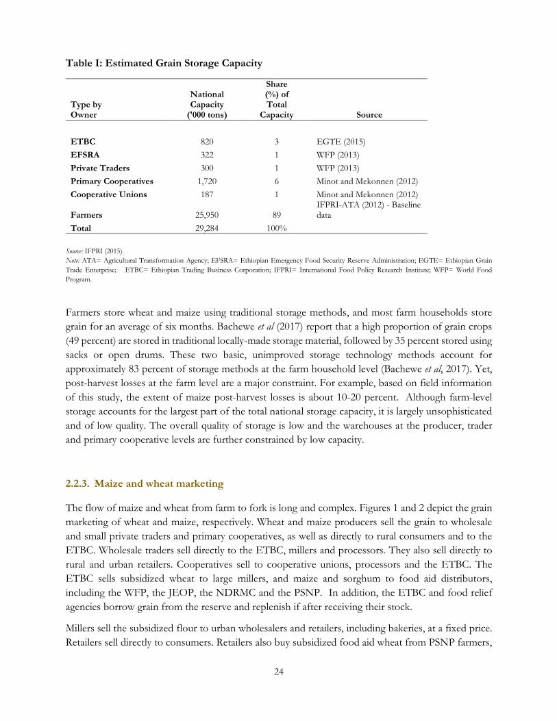
24

Table I: Estimated Grain Storage Capacity

Type by Owner

National Capacity

('000 tons)

Share (%) of Total

Capacity Source

ETBC 820 3 EGTE (2015)

EFSRA 322 1 WFP (2013)

Private Traders 300 1 WFP (2013)

Primary Cooperatives 1,720 6 Minot and Mekonnen (2012)

Cooperative Unions 187 1 Minot and Mekonnen (2012)

Farmers 25,950 89

IFPRI-ATA (2012) - Baseline data

Total 29,284 100%

Source: IFPRI (2015).

Note: ATA= Agricultural Transformation Agency; EFSRA= Ethiopian Emergency Food Security Reserve Administration; EGTE= Ethiopian Grain

Trade Enterprise; ETBC= Ethiopian Trading Business Corporation; IFPRI= International Food Policy Research Institute; WFP= World Food

Program.

Farmers store wheat and maize using traditional storage methods, and most farm households store

grain for an average of six months. Bachewe et al (2017) report that a high proportion of grain crops

(49 percent) are stored in traditional locally-made storage material, followed by 35 percent stored using

sacks or open drums. These two basic, unimproved storage technology methods account for

approximately 83 percent of storage methods at the farm household level (Bachewe et al, 2017). Yet,

post-harvest losses at the farm level are a major constraint. For example, based on field information

of this study, the extent of maize post-harvest losses is about 10-20 percent. Although farm-level

storage accounts for the largest part of the total national storage capacity, it is largely unsophisticated

and of low quality. The overall quality of storage is low and the warehouses at the producer, trader

and primary cooperative levels are further constrained by low capacity.

2.2.3. Maize and wheat marketing

The flow of maize and wheat from farm to fork is long and complex. Figures 1 and 2 depict the grain

marketing of wheat and maize, respectively. Wheat and maize producers sell the grain to wholesale

and small private traders and primary cooperatives, as well as directly to rural consumers and to the

ETBC. Wholesale traders sell directly to the ETBC, millers and processors. They also sell directly to

rural and urban retailers. Cooperatives sell to cooperative unions, processors and the ETBC. The

ETBC sells subsidized wheat to large millers, and maize and sorghum to food aid distributors,

including the WFP, the JEOP, the NDRMC and the PSNP. In addition, the ETBC and food relief

agencies borrow grain from the reserve and replenish if after receiving their stock.

Millers sell the subsidized flour to urban wholesalers and retailers, including bakeries, at a fixed price.

Retailers sell directly to consumers. Retailers also buy subsidized food aid wheat from PSNP farmers,

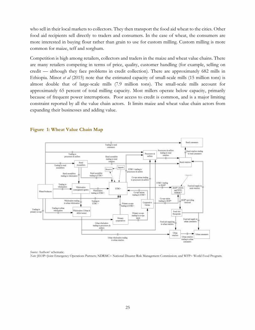
25

who sell in their local markets to collectors. They then transport the food aid wheat to the cities. Other

food aid recipients sell directly to traders and consumers. In the case of wheat, the consumers are

more interested in buying flour rather than grain to use for custom milling. Custom milling is more

common for maize, teff and sorghum.

Competition is high among retailers, collectors and traders in the maize and wheat value chains. There

are many retailers competing in terms of price, quality, customer handling (for example, selling on

credit — although they face problems in credit collection). There are approximately 682 mills in

Ethiopia. Minot et al (2015) note that the estimated capacity of small-scale mills (15 million tons) is

almost double that of large-scale mills (7.9 million tons). The small-scale mills account for

approximately 65 percent of total milling capacity. Most millers operate below capacity, primarily

because of frequent power interruptions. Poor access to credit is common, and is a major limiting

constraint reported by all the value chain actors. It limits maize and wheat value chain actors from

expanding their businesses and adding value.

Figure 1: Wheat Value Chain Map

Source: Authors’ schematic. Note: JEOP=Joint Emergency Operations Partners; NDRMC= National Disaster Risk Management Commission; and WFP= World Food Program.

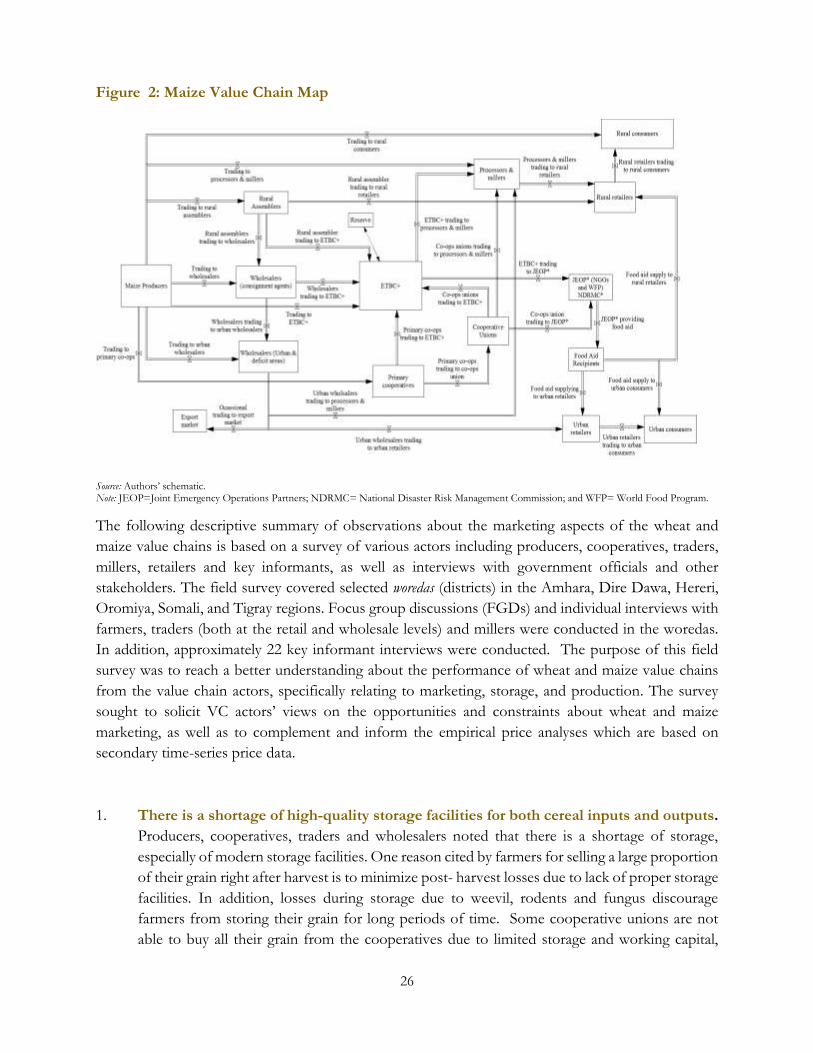
26

Figure 2: Maize Value Chain Map

Source: Authors’ schematic. Note: JEOP=Joint Emergency Operations Partners; NDRMC= National Disaster Risk Management Commission; and WFP= World Food Program.

The following descriptive summary of observations about the marketing aspects of the wheat and

maize value chains is based on a survey of various actors including producers, cooperatives, traders,

millers, retailers and key informants, as well as interviews with government officials and other

stakeholders. The field survey covered selected woredas (districts) in the Amhara, Dire Dawa, Hereri,

Oromiya, Somali, and Tigray regions. Focus group discussions (FGDs) and individual interviews with

farmers, traders (both at the retail and wholesale levels) and millers were conducted in the woredas.

In addition, approximately 22 key informant interviews were conducted. The purpose of this field

survey was to reach a better understanding about the performance of wheat and maize value chains

from the value chain actors, specifically relating to marketing, storage, and production. The survey

sought to solicit VC actors’ views on the opportunities and constraints about wheat and maize

marketing, as well as to complement and inform the empirical price analyses which are based on

secondary time-series price data.

1. There is a shortage of high-quality storage facilities for both cereal inputs and outputs.

Producers, cooperatives, traders and wholesalers noted that there is a shortage of storage,

especially of modern storage facilities. One reason cited by farmers for selling a large proportion

of their grain right after harvest is to minimize post- harvest losses due to lack of proper storage

facilities. In addition, losses during storage due to weevil, rodents and fungus discourage

farmers from storing their grain for long periods of time. Some cooperative unions are not

able to buy all their grain from the cooperatives due to limited storage and working capital,

27

which creates problems with primary cooperatives and their members. To meet demand, some

cooperative unions rent storage space from the private sector. Sometimes, primary

cooperatives sell grain at reduced prices to the unions due to limited cooperative storage.

However, field observations also reveal that primary cooperatives primarily store inputs, such

as fertilizers and seeds, to distribute to farmers.

2. The lack of coordination and planning among grain importing entities leads to sub-

optimal utilization of the existing public storage system. Discussions with key informants

reveal that there is a lack of coordination and planning among the key entities involved in the

importation of wheat, including the ETBC, as well as among the JEOP, the WFP and the

NDRMC. Interviews with the NDRMC indicate that the swapping of warehouses within the

public storage system is weak. Consequently, at times some public storage warehouses are

empty for months, while others are overfilled and not able to store more grain. In addition,

each entity imports grain for its own program, with little synchronization with the other

importers. This sometimes results in large grain shipments arriving at the same time at the port

in Djibouti, leading to congestion and delays in delivering the shipment. Furthermore, the

simultaneous arrival of the imported wheat in the country affects local prices.

3. Most of the existing single-structured storage facilities do not meet the multi-purpose

storage needs at the farm, cooperative and union levels. Ideally, what the farmers want is

separate storage facilities for grain, fertilizers and improved seeds. Currently, due to the shortage, the

farmers use the same facility to store farm inputs and outputs simultaneously or alternatively.

This can create potential food safety and health problems, as well as logistical issues due to the

small storage capacity. In addition to grains, farmers grow different crops requiring storage.

However, mostly one storage structures are built with no capacity to manage the storage of

several crops. The storage structures are primarily used for storing dry grain, and there are no

storage structures for fruits and vegetables. At the union level, there are different needs for

storage including storing grains, fertilizers, chemicals and seeds. However, most unions only

have one storage structure, and this creates a challenging situation when they mix grains with

other things.

4. Lack of trust in the maize and wheat value chains is pervasive; it discourages the use

of cooperative and private storage facilities by producers. A consistent issue raised by

farmers in most of the regions related to storing grain with private warehouses and cooperatives

is lack of trust. There is a lack of trust in the capacity of cooperatives to keep their grain in good

condition, given the quality standards of the existing infrastructure. Although producers are

aware of the storage losses on farms, they are reluctant to store grain elsewhere with private

storage owners. Farmers do not trust their grain with anyone else. In other cases, the warehouse

owners do not want to take the responsibility for storing grain for several individual farmers

due to potential theft and storage losses. Although many farmers are aware of and appreciate

the benefits of cooperatives, many noted corruption by some cooperatives. This discourages

them from selling and storing their grain with the primary cooperatives. There is also mistrust

between the primary and union cooperatives, mainly due to the lack of storage space when

28

there is oversupply after bumper harvests. When unions cannot buy all the grains from the

primary cooperatives, the primary cooperatives then dispose of it in the local markets by selling

it to traders at lower prices or by reselling the grain to members at the prices procured from

the producers.

5. Most farmers cannot use primary cooperatives’ storage facilities for temporal arbitrage.

Due to cooperative by-laws, most farmers cannot use cooperative storage to store grain and

then sell it later when prices are expected to rise. Most cooperatives do not provide storage

services for individual farmers. Only a few cooperatives provide storage services to members.

For example, in Galama, the primary cooperative stores grain for members by marking the

grain sacks with the name of the cooperative member. The focus of most cooperatives is service

provision (especially related to inputs, such fertilizers and seeds), with limited profit orientation.

6. Producers sell a negligible amount of wheat and maize through the primary

cooperatives. Field data and information show that producers sell a small fraction of their

marketable output through cooperatives. Consistent with this observation, a recent AGP 2

baseline survey6 of 10,924 randomly selected households reveals that farmers only sell 2.6

percent of their crops through cooperatives. The data further reveal that households sell 1.9

percent (wheat) and 3.8 percent (maize) of their output through cooperatives, as compared with

66 percent (wheat) and 64 percent (maize) sold through private traders. This observation is

consistent with previous research (Abate et al, 2015; EDRI 2017; and Minot et al, 2015) into

wheat and maize marketing in Ethiopia. The FCA estimates are higher noting that producers

sell approximately 10-11 percent of their agricultural output through cooperatives.

There are several reasons why producers sell less of their marketable output through

cooperatives. First, most farmers noted that the cooperatives buy immediately after harvest over a short

window of time when prices are low. In addition, the primary cooperatives’ management lacks

flexibility in setting prices because the price is decided by the board. In this regard, there is a

time lag in price setting, which means that the cooperatives could lose business opportunities.

Second, and more importantly, many producers view the cooperatives as an unreliable marketing

outlet for the farmers in terms of the price they offer, the amount they purchase, the consistency

of purchasing, and the time length of purchasing. Third, most primary cooperatives have

financial constraints and poor market linkages to purchase the desired quantity from their

members. As such, their purchasing pattern and quantities are limited and unpredictable. In

addition, because some cooperatives decisions about purchasing are influenced by external

buyers’ like the WFP, the ad hoc market participation of these external buyers results in

inconsistent buying patterns of cooperatives from their members. Consequently, most

cooperatives do not satisfy the farmers’ needs in terms of the quantity they buy, the continuity

of the market outlet and the price they offer. This further contributes to high levels of side-selling

6 Agricultural Growth Project/AGP II Baseline Draft Survey Report (EDRI, 2017). The data covers four regions including high surplus grain areas

29

by cooperative members because they prefer to sell directly to traders who offer better prices,

sustainable purchases and cash advances. Increasing marketing through cooperatives is an

important ingredient to achieving agricultural commercialization and transformation in

Ethiopia. However, field data and interviews reveal that most producers do not sell much

marketable output through cooperatives. Thus, cooperatives provide an important service on

the input side, but their output marketing function is weak.

7. Most farmers sell immediately after the harvest to meet their financial obligations,

which are usually due then. Field observations and interviews reveal that most farmers sell at

harvest time at lower prices due to cash shortages. For example, in Shashemene in West Arsi,

about 60 percent of the farmers sell immediately after the harvest — not because of storage

problems — but more because of the need for cash to meet financial obligations which are due

right after the harvest. Although there are microfinance service providers in some areas, there

are several problems with their use. First, the timing of the loan provision is not designed in

such a way as to prevent the farmers from selling their crops after the harvest. Second, debt

collection is undertaken right after the harvest, which compels the farmers to sell assets. Third,

producers mostly use the loans from microfinance institutions for consumption purposes, and

not for productive investments. Furthermore, producers mostly sell to the traders on credit in

advance of harvest time. They then pay in kind at cheap rates immediately after the harvest

when the price is the lowest of the season. Consequently, most producers do not benefit from

better prices because of untimely sales and weak bargaining power.

8. The lack of transparency in price discovery and asymmetric price information in cereal

marketing contributes to many uncertainties in the maize and wheat value chain. Many

actors in the maize and wheat value chain emphasize that there is a lack of transparency

regarding how wheat and maize prices are determined. In addition, prices are not announced

to the grain value chain actors. Farmers noted that they do not have clear market information

in the distant wholesale markets. They also noted that farmers-traders influence the price of

wheat by spreading untruthful rumors that the supply of wheat is going to increase due to food

aid wheat, so they pay lower/constant prices to the farmers. For example, farmers in the high

producing area of Arsi indicated that the food aid wheat is depressing the market prices for

wheat because traders spread the news of the food aid wheat to keep the prices low. Focal

group discussion with farmers in Eteya Town (Arsi zone) reveal that farmers are not informed

about cereal market prices for important destination markets, such as Adama and Addis Ababa.

They obtain market information from brokers. However, because of a conflict of interest, it is

hard to expect complete disclosure of market information by the brokers to the farmers.

Furthermore, interviews with government officials reveal that cereal prices are determined

internally and are not announced to VC actors. Key factors considered in determining the grain

prices are the prevailing open market cereal prices and the expected supply. The cost of

production is not clearly factored into cereal price determination. The ETBC makes the final

price decision at its head office, and announces prices in localities during purchasing, and when

prices are volatile. As such, it gives the mandate to its agents to determine the price. In addition,

30

information on the prices at which the processors are buying is not available and communicated

to all stakeholders. Thus, there is a clear need to establish a grain marketing information system

which includes price information, and forecasting on expected grain supplies based on reliable

data and methods.

9. Uncertainties about the quantity and the timing of distribution of subsidized wheat and

maize negatively affects local prices. Farmers in high producing areas like Arsi revealed

that the government distributes subsidized wheat to wheat flour mills at lower prices when

there is no shortage of wheat in the market. Consequently, this sends the wrong market signals,

adversely affecting the smooth functioning of the wheat market. This is consistent with

sentiment by government officials that the data about the expectations regarding the cereal

supply are not reliable. Furthermore, many farmers, especially in grain deficit regions, noted

that flour mills prefer to buy the subsidized imported wheat before they buy the local product

because it is cheaper and more uniform in quality. Wheat retailers in Tigray and other regions

buy subsidized wheat flour from food aid recipients at cheaper prices. Farmers revealed a

frustration that the government is urging producers to increase their production, whereas the

(untimely) distribution of cheaper subsidized wheat negatively affects their local markets. Thus,

there is a need to clearly and reliably determine the marketable surplus for maize and wheat to

plan investments in storage, processing and other logistical functions necessary for a well-

functioning cereal marketing system.

10. Unclear and arbitrary tax practices are turning cereal wholesale traders into retailers in

some regions. Field information based on focus group discussions with wholesale traders in

the Amhara region reveal an emerging trend of tax practices, resulting in disincentives in the

wholesale trading business. The tax is based on the amount of stock held at the time of a visit

by the tax official. It is not based on the business turnover. Since the stock might be held for a

very long time and the price can go up or down, the wholesalers reported price fluctuations

resulting in high variability in the traders’ income. In this context, there is a strong probability

for over-taxing when the tax is based solely on the stock level. Hence, holding large stocks at

the traders or wholesalers shed is a condition for imposing higher taxes by the tax authorities.

Consequently, traders avoid holding large stocks or unloading from trucks in public. However,

tax authorities have agents working for them who provide immediate reports of the location

whenever they see the unloading of cereals from trucks outside the premises of the traders.

Because of this tax system, wholesalers are not receiving the bulk transport of cereals from

other regions. Indeed, they are now more interested in holding small stocks, and in retailing

rather than wholesaling. Wholesale trading is an important function for commodity flows

between surplus producing and cereal deficit regions. Unclear tax policies can weaken this link,

restrict spatial arbitrage and hinder the effective functioning of cereal markets. They also reduce

incentives for the private sector to invest in storage facilities.

11. Cheating is a common phenomenon in the maize and wheat marketing chain. Producers

in Tigray and other deficit areas noted that due to the influx of cheaper subsidized wheat from

the government, the millers are not honoring their contracts with the unions and subsequently

31

break them. Contractual defaults were also reported at the cooperative level, leading to a

decrease in farmers’ interest in working with cooperatives. At the same time, cooperative

members engage in side-selling, as they prefer to sell to traders because they receive better

prices and can rely on more consistent purchasing. A farmers group interview in West Arsi

reveals that farmers prefer to sell to the farmer-trader in their area because the traders in town

cheat on the weight. The traders adjust the weight downward by decreasing the weight of the

grain by 5 to 10 kilograms (kg) per 100 kg weight of grain delivered by the farmers. It is almost

a common practice that the farmers mix grain with impurities to increase the weight of the

grain because they know that the traders will cheat on the weight. Further, some cooperatives

are strict in terms of quality and weight of the grain. For example, the cooperative in Bako Tibe

is strict about quality and does not buy if there is any weevil infestation. As such, it only pays

for 95 kg of maize to account for some losses. However, the traders would buy even the weevil-

infested maize and pay for 100 kg maize. They would then mix low quality maize with the

higher quality maize. With the way that the business is conducted between traders and

producers, the overall consistency of the average quality of grain delivered to the retailers and

processors is poor. The retailers need to clean the grains more before they sell to their

customers; otherwise, the consumers will not be willing to buy from the retailers.

In a focus group survey, producers in a high wheat producing zone (Bale) indicated that, in

some cases, the procurement and marketing practices of the ETBC are prone to bribes. Some

ETBC agents receive about 20 Birr/quintal to accept deliveries from the producers or traders,

and return the truck load if the payment is not made. One consequence of this conduct is that

ETBC agents do not pay careful attention to quality, and will accept any wheat delivered by the

traders. Since ETBC agents do not prefer to buy from the farmers with small plots, the small

farmers sell to traders who then aggregate the grains and sell them to the ETBC. However, the

traders mix different qualities and sell it to ETBC agents. The traders are reported to pay up to

300 Birr per truck load in bribes to ETBC staff for their delivery to be accepted.

Overall, these adverse selection problems reduce the consistency of the average quality of

locally procured wheat, leading processors to also prefer imported wheat. Thus, there is a need

for regular third-party oversight of the weight and quality inspection process.

12. Poor regulation and enforcement of quality and standards prevail in the marketing of

maize and wheat. Although many buyers assign grades, there are no formal maize and wheat

grain standards. So too, there is no formal and consistent quality enforcement at the different

nodes of both value chains. The quality requirements by cooperatives are higher, but the quality

of the grain is examined only physically for breakage and obvious physical impurities. There are

no quality checks for moisture content or for storing the grain at the appropriate moisture and

temperature levels. In this context, many cooperatives do not provide important

preconditioning services, such as sorting, drying, and grading before storing the grain. Traders

handle low quality wheat and maize and mix grain of different qualities, reducing the average

quality flowing through the value chain. Processors noted that the unions do not provide a

continuous supply of good quality grain. In East Wolega, for example, some unions are proving

32

training to members regarding the quality management of maize. Many millers noted that the

imported wheat flour is of high quality, especially in terms consistency. As a result, apart from

the imported wheat being cheaper, many millers and retailers note that the subsidized wheat

has more uniform quality.

Overall, although farmers can produce good quality bread, pasta wheat and maize flour, the

weak market linkages and quality enforcement do not encourage farmers to invest more in

quality. However, ATA’s work in the wheat value chain and market linkages with factories was

successful for the Gololcha Union (Arsi Zone). More effort will be needed to create such

market linkages. Producers need to be convinced that they will obtain a better price through

such linkages than in the open market. As such, they would be motivated to invest more in the

production of high quality grain.

13. Some medium-to-large processors do not source locally and rely on imported

subsidized wheat. In low wheat producing regions like Tigray, some large millers noted that

they largely depend on the government-subsidized imported wheat as a raw material for their

milling. Since the local wheat is more expensive (when buying and selling flour), the company

is not interested in obtaining the raw wheat locally. Thus, the raw wheat used for processing is

entirely imported or supplied by the government through the ETBC. A large industrial miller

used to import wheat from Addis Ababa, but with the subsidy, the miller stopped the importation of wheat as

it could not compete with subsidized wheat flour or bread. Other small-to-medium millers in Mekele

noted that the demand for wheat from Amhara and other regions to Tigray is insignificant.

Therefore, they only procure wheat occasionally from within the region. The demand for wheat

in Mekele is for industrial milling, which is mostly satisfied by imported, subsidized wheat.

Traders in Dessie noted that subsidized wheat is of good quality and cheaper. Hence, sourcing

wheat from a distant or local market is not profitable. Flour mills buy food-aid wheat as much

as possible to meet their requirements. They then buy from the cooperatives as a last resort if

they cannot obtain sufficient supplies of food aid wheat. Overall, local producers are frustrated

that subsidized wheat is weakening their market potential to supply to local processors, retailers

and other buyers.

A key assumption of the wheat subsidy is that the subsidized wheat flour does not leak into the

open market if well targeted. However, there is a strong incentive to do just that because the

open market price of wheat flour is significantly higher than the subsidized wheat flour. For

example, at the time of field work, the price of wheat flour was 1,200 Birr per quintal in the

open market, which is significantly higher than the subsidized wheat flour price of 726 Birr per

quintal. Field interviews with retailers and traders reveal that many retailers and traders buy

subsidized wheat from food aid household recipients. Hence, there is a need for careful

inspection and regulation of the distribution of subsidized wheat. In addition, careful

consideration is also required regarding the right mix and appropriateness of food versus cash

transfers to food insecure households in some locations where recipients are selling their cereals

to other consumers, retailers and traders.

33

There are now more direct shipments of maize from the production areas to the

consumption areas, bypassing the traditional transshipment wholesale market in Addis

Ababa. This is indicative of the improvements in road infrastructure, the availability of trucks

at competitive prices, and improvements in cereal traders’ networking capacity due to increased

access to mobile phones. In deficit areas (Wallale-Jijiga) of the Harar and Somali regions, large

wholesale traders import maize directly from other areas, especially Wollega. There is also an

emerging trend of importing hubs, where some private investors are building modern

warehouses and importing maize directly from Wollega. They then stock it for local distribution

and exports to more distant places in the zone and other regions like Jijiga.

3. Conceptual Framework and Empirical Strategy

3.1 A conceptual framework for cereal market performance analysis

In Ethiopia, grain production is dominated by geographically-dispersed smallholder farmers. There

are clear regional variations in the volume of different grains produced in the country. Some of the

major consumption markets are in grain deficit regions, relying on grain imports from the surplus-

producing regions or imports — giving rise to both temporal and inter-regional grain trading

opportunities. Since liberalization in 1991, the grain marketing system in Ethiopia has been

characterized by the coexistence of the state-owned marketing agency, cooperative marketing and

private sector grain trade, each with different resources and capacities to engage in the market. Given

this general context, in this study, the performances of maize and wheat markets are evaluated based

on statistical and econometric models using historical time series price data collected in different

markets and at different marketing levels (producer, wholesale and retail). This section provides a brief

discussion of the conceptual framework guiding the statistical and econometric analyses and

interpretation of cereal market performance in Ethiopia.

Grain marketing involves several different functions such as storage, transportation, processing and

arbitrage. The evaluation of marketing system performance is essential to identifying the defects in the

marketing system, as well as to suggesting possible ways of improvement. Pricing efficiency is one of

the measures of the performance of agricultural marketing systems based on the economic model of

perfectly competitive markets. It is concerned with how the market allocates resources to their best

use, and coordinates production and marketing process to obtain the maximum output. It is indicated

that “pricing efficiency is less than perfect when prices fail to (1) fully represent consumer preferences;

(2) direct resources from lower to higher values uses; or (3) coordinate the buying and selling activities

of farmers, marketing firms and consumers” (Kohls and Uhl, 1993). The efficiency of a given

agricultural marketing system is influenced by several factors such as competition, government

marketing policy, and marketing infrastructure development.

Some of the key variables used in evaluating the pricing efficiency of agricultural marketing systems

are based on a perfectly competitive market model. These include: price levels, price variability,

marketing margins, and the degree of market integration. It is possible to classify marketing margins

into three categories: spatial, temporal, and form change, that is, the marketing margin for the product.

34

In terms of spatial marketing margins, when there are no impediments to trading between two regions,

with trade, the price difference will equal transfer costs; with no trade, it will be less than or equal to

transfer costs (Tomek and Robinson, 1993). This is based on the concept of the spatially-competitive

equilibrium model; deviations from these outcomes are assumed to indicate inefficiencies.

In the case of temporal price margins, the increase in the prices of physical commodities from one-

time period to the next is assumed to be equal to the costs of storage from one period to the next,

plus “normal profits” for the traders (Delgado, 1986). This is based on the concept of inter-temporal

competitive market equilibrium. Delgado (1986) suggests that the implication of high inter-temporal

price variabilities (seasonal price spreads) — independent of storage and transaction costs — are

indications of inefficiencies in the marketing system. The marketing margin for the product form

changes must also be reflected in the processing costs for an efficient market.

Small farmers in most developing countries are responsive to prices. Consequently, agricultural prices

play an important role in achieving the efficient allocation of resources (Ahmed and Mellor, 1990;

Timmer, 1987). In this context, Timmer (1987) indicates that market performance and its welfare

impact depend on the efficiency with which markets generate and transmit price signals.

The level of prices determines the profitability of farmers’ investments. Hence, their incentive to invest

is also important to the improvement of the national economy. The level of prices also determines

what proportion of the product must be sold in the market by the farm households to meet their

financial obligations, as well as for the purchase of farm inputs. In the case of food shortages in the

family, price levels affect farmers’ capacity to buy in the market, thereby influencing farmers’ food

security. Price level also affects urban consumers’ purchasing power, and their food security situation

as well.

Price variability or stability is related to the pattern of price level changes over time, which might be

predictable or unpredictable. In the case of prices varying in an unpredictable pattern, the means and

variance of prices will change from time to time. However, in the case of stable or less variable prices,

there is no significant change in the means and variance over time. As such, the price will vary around

known trends or it may vary around mean values with constant variances. However, it is argued that

in the efficient market, the prices should vary to account for the changes in the costs of marketing

services, such as transportation and storage costs (Delgado, 1986).

Price stability can be an important efficiency indicator of agricultural market performance. Unstable

and unpredictable prices will result in insecure farm incomes, and this complicates the farmers

planning process (Kohls and Uhl,1990). Thus, under the condition of highly variable or unstable prices

which are unpredictable, the role of prices in allocating resources to their best use is minimized. The

accuracy by which price changes can be predicted is important for both food producing and

consuming households to adjust their sale and storage strategies to achieve food consumption

objectives (Sahn and Delgado,1989). It is also found that the risk of price instability tends to decrease

aggregate supply and increase marketing margins (Brorsen et al, 1987).

The variability of price can be analyzed at different levels, including the producer, wholesale and retail

levels. These analyses on price responsiveness at different levels in the marketing channel can provide

35

an indicator of market performance (Pick et al, 1990). If the market is efficient, it is expected that there

would be a very fast and symmetric transmission of price changes from one level to another. The same

also applies for efficiently linked spatial markets. Different market levels are expected to have similar

levels of variability measures.

Market integration as a test of market performance is based on the concept that markets are integrated

only if their prices do not behave independently — and that changes in prices at one marketing level

are reflected at all other levels (Ahmed, 1998; Faminow and Benson, 1990). Heytens (1986) also

indicates that in an “efficiently integrated” marketing system, there will be positive price correlation

over time among prices at different market locations. Specifically, there is no price divergence among

integrated markets. If two markets are integrated, the price difference between the two markets equals

the transfer costs (Ravallion, 1986).

Market integration through infrastructure development is expected to reduce temporal price variability

and spatial price disparities (Fafchamps, 1992). However, markets that are not well integrated may

convey inaccurate price information that might also distort producer marketing decisions and

contribute to inefficient product movements (Goodwin and Schreder, 1991). The other factors

affecting market integration include: market information and knowledge; the ability to respond to

market opportunities; and the resources and ease with which produce can be moved from one market

to another (Southworth et al, 1979). Thus, the spatial market efficiency also has implications for food

security.

Given this conceptual framework, this section presents the various statistical econometric methods

used to analyze the fluctuations of maize and wheat prices over time and space. Some of the key

features modeled include: (1) maize and wheat price volatilities to gauge the level of risk in their

respective markets; (2) seasonal price movements to assess the level of temporal arbitrage

opportunities and efficiencies; and (3) spatial price linkages to assess the level of spatial arbitrage

opportunities, efficiencies and extent of market integration.

3.2. Measuring the levels and variability of maize and wheat prices

3.2.1 Analyzing maize and wheat price levels and variability

3.2.1.1 Overall maize and wheat price fluctuations

In general, the cereal price fluctuation over time can be disaggregated into two major components —

predictable and unpredictable components. The important question then becomes: Which component

plays an important role in the overall price fluctuation? The level of uncertainty or unpredictability is

usually associated with the riskiness of cereal markets. The risks present in the marketing system

prevent the realization or occurrence of advantageous spatial and temporal arbitrage opportunities.

However, it can also prevent optimal investments in production, and distribution marketing activities.

Therefore, it is important to discern the level of unpredictability or uncertainty present in the cereal

price fluctuations. This data will help to inform strategies and polices to prevent, mitigate or reduce

such price risks.

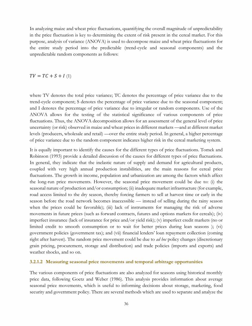
36

In analyzing maize and wheat price fluctuations, quantifying the overall magnitude of unpredictability

in the price fluctuation is key to determining the extent of risk present in the cereal market. For this

purpose, analysis of variance (ANOVA) is used to decompose maize and wheat price fluctuations for

the entire study period into the predictable (trend-cycle and seasonal components) and the

unpredictable random components as follows:

𝑇𝑉 = 𝑇𝐶 + 𝑆 + 𝐼 (1)

where TV denotes the total price variance; TC denotes the percentage of price variance due to the

trend-cycle component; S denotes the percentage of price variance due to the seasonal component;

and I denotes the percentage of price variance due to irregular or random components. Use of the

ANOVA allows for the testing of the statistical significance of various components of price

fluctuations. Thus, the ANOVA decomposition allows for an assessment of the general level of price

uncertainty (or risk) observed in maize and wheat prices in different markets —and at different market

levels (producers, wholesale and retail) —over the entire study period. In general, a higher percentage

of price variance due to the random component indicates higher risk in the cereal marketing system.

It is equally important to identify the causes for the different types of price fluctuations. Tomek and

Robinson (1993) provide a detailed discussion of the causes for different types of price fluctuations.

In general, they indicate that the inelastic nature of supply and demand for agricultural products,

coupled with very high annual production instabilities, are the main reasons for cereal price

fluctuations. The growth in income, population and urbanization are among the factors which affect

the long-run price movements. However, the seasonal price movement could be due to: (i) the

seasonal nature of production and/or consumption; (ii) inadequate market infrastructure (for example,

road access limited to the dry season, thereby forcing farmers to sell at harvest time or early in the

season before the road network becomes inaccessible — instead of selling during the rainy season

when the prices could be favorable); (iii) lack of instruments for managing the risk of adverse

movements in future prices (such as forward contracts, futures and options markets for cereals); (iv)

imperfect insurance (lack of insurance for price and/or yield risk); (v) imperfect credit markets (no or

limited credit to smooth consumption or to wait for better prices during lean seasons ); (vi)

government policies (government tax); and (vii) financial lenders’ loan repayment collection (coming

right after harvest). The random price movement could be due to ad hoc policy changes (discretionary

grain pricing, procurement, storage and distribution) and trade policies (imports and exports) and

weather shocks, and so on.

3.2.1.2 Measuring seasonal price movements and temporal arbitrage opportunities

The various components of price fluctuations are also analyzed for seasons using historical monthly

price data, following Goetz and Weber (1986). This analysis provides information about average

seasonal price movements, which is useful to informing decisions about storage, marketing, food

security and government policy. There are several methods which are used to separate and analyze the

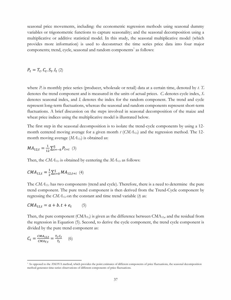
37

seasonal price movements, including: the econometric regression methods using seasonal dummy

variables or trigonometric functions to capture seasonality; and the seasonal decomposition using a

multiplicative or additive statistical model. In this study, the seasonal multiplicative model (which

provides more information) is used to deconstruct the time series price data into four major

components; trend, cycle, seasonal and random components7 as follows:

𝑃𝑡 = 𝑇𝑡. 𝐶𝑡. 𝑆𝑡. 𝐼𝑡 (2)

where Pt is monthly price series (producer, wholesale or retail) data at a certain time, denoted by t. Tt

denotes the trend component and is measured in the units of actual prices. Ct denotes cycle index, St

denotes seasonal index, and It denotes the index for the random component. The trend and cycle

represent long-term fluctuations, whereas the seasonal and random components represent short-term

fluctuations. A brief discussion on the steps involved in seasonal decomposition of the maize and

wheat price indices using the multiplicative model is illustrated below.

The first step in the seasonal decomposition is to isolate the trend-cycle components by using a 12-

month centered moving average for a given month t (CMA12,t) and the regression method. The 12-

month moving average (MA12,t) is obtained as:

𝑀𝐴12,𝑡 =1

12∑ 𝑃𝑡+𝑖

5𝑖=−6 (3)

Then, the CMA12,t is obtained by centering the MA12,t as follows:

𝐶𝑀𝐴12,𝑡 =1

2∑ 𝑀𝐴12,𝑡+𝑖

1𝑖=0 (4)

The CMA12,t has two components (trend and cycle). Therefore, there is a need to determine the pure

trend component. The pure trend component is then derived from the Trend-Cycle component by

regressing the CMA12,t on the constant and time trend variable (t) as:

𝐶𝑀𝐴12,𝑡 = 𝑎 + 𝑏. 𝑡 + 𝑒𝑡 (5)

Then, the pure component (CMAT,t) is given as the difference between CMA12,t and the residual from

the regression in Equation (5). Second, to derive the cycle component, the trend cycle component is

divided by the pure trend component as:

𝐶𝑡 =𝐶𝑀𝐴12,𝑡

𝐶𝑀𝐴𝑇,𝑡=

𝑇𝑡.𝐶𝑡

𝑇𝑡 (6)

7 As opposed to the ANOVA method, which provides the point estimates of different components of price fluctuations, the seasonal decomposition

method generates time-series observations of different components of price fluctuations.

38

The seasonal index is obtained as follows. First, the seasonality factor is computed by dividing the

actual price series by the centered moving average; hence, the name ratio-to-moving average method:

𝑆𝑡𝐼𝑡 =𝑃𝑡

𝐶𝑀𝐴12,𝑡=

𝑇𝑡.𝐶𝑡.𝑆𝑡.𝐼𝑡

𝑇𝑡.𝐶𝑡 (7)

Then, to calculate the pure seasonal component for each month, we simply sum and average the

indices of the same month over all years (N). For example, the average of all jth month indices is

computed as follows:

𝑆�̅� =1

𝑁∑ 𝑆𝑗𝑡

𝑁𝑡=1 ; 𝑗 = 1,2,3, … ,12; 𝑡 = 1,2,3, … , 𝑁 (8)

where j denotes the month (1=January, 2=February, 3=March, etc.); t denotes the year. The

summation of a given month is over the entire study period. The final step is to calculate the random

component as:

𝐼𝑡 =𝑆𝑡.𝐼𝑡

𝑆𝑡 (9)

Finally, the purely seasonal component is obtained as:

𝑆𝑡 =𝑆𝑡.𝐼𝑡

𝐼𝑡 (10)

The stability of the pattern of seasonal price movement is analyzed by fitting the time trend regression

to the pure seasonal index. The significant coefficient on the time trend variable indicates the change

in pattern of seasonal price movement over the time. The standard deviation of the seasonal index

also shows the variability of the seasonal index.

Finally, the Grand Seasonal index (GSIj) for jth month utilizes the entire historical price dataset and

satisfies the condition that all indices add up to 12. This is given as:

𝐺𝑆𝐼𝑗 = 𝑆�̅�.12

∑ 𝑆𝑗 (11)

In relation to grain storage, the key parameter which can be derived from the seasonal decomposition

of cereal prices is the seasonal price spread. The seasonal price spread is given as the difference

between the highest and the lowest seasonal index. This spread can also be expressed as the ratio to

the lowest seasonal index:

𝐺𝑆𝑅 =𝐻𝑖𝑔ℎ𝑒𝑠𝑡 𝐺𝑆𝐼−𝐿𝑜𝑤𝑒𝑠𝑡 𝐺𝑆𝐼

𝐿𝑜𝑤𝑒𝑠𝑡 𝐺𝑆𝐼∗ 100 (12)

This ratio is also called gross storage return (GSR) and measures the average seasonal price movement

based on historical price data, which shows the potential for temporal arbitrage (Tshirely 1995).

However, the seasonal price spread alone cannot be used to assess storage profitability in making

storage decisions. It needs to be compared with the costs of storage. Under the competitive market

39

conditions, the profit maximization rule by different economic agents gives rise to the temporal

arbitrage condition given as (Wright 2011):

1−𝜋

1+𝑟𝐸𝑡𝑃𝑡+1 ≤ 𝑃𝑡 + 𝐶𝑡 ; 𝑆𝑡𝑜𝑐𝑘 ≥ 0 (13)

where 𝜋 denotes the assumed storage loss or grain product depreciation over the storage period; r

denotes the interest on capital used to buy the grain (Pt) and to pay for the storage rent (Ct); and EtPt+1

denotes the expected price of grain at the end of storage period (t+1). The temporal arbitrage

condition states that for storage to occur, the discounted future price must be less than or equal to the

current price —plus the costs of storage. With competition, the equality constraint holds. It is

important to note that in the absence of historical data on storage costs, the efficiency of existing

storage can be evaluated by computing the return (𝜑) required to break even given the current assessed

grain storage loss and the market interest rate by solving for 𝜑 in the following equation:

1−𝜋

1+𝑟=

1

1+𝜑 (14)

Then, accounting for the appropriate storage period, the breakeven return can be compared with the

average return to storage for a given period. This can be done by utilizing the monthly return

computed from the historical price data and assessing whether the realized returns are below or above

the breakeven return — indicating whether the realized returns are small, excessive or reasonable. For

example, if the storage period is for six months and the computed average monthly return is 2 percent,

then the return for the six-month storage period is given as 12 percent (6*2 percent). Then this return

is compared with the breakeven return rate for six months (𝜑 ∗ 6). It should also be noted that

reducing storage losses increases the profitability of storage.

The constructed seasonal price indices can be used to inform storage or marketing decisions at harvest

time by enabling forecasts about the future price based on the harvest time price. For example, the

forecast for a given month (at the end of the planned storage period) in the future can be determined

as follows. First, the seasonal average price is obtained by dividing the harvest month price by its

index. Second, the forecasted price for a given month in the future is obtained by multiplying the

seasonal average price by the index of the forecast month. This procedure allows the producers or

private traders to estimate the expected price increase in the lean season. Thus, the computed expected

price increase can be compared to the costs of on-farm storage. These include grain depreciation and

other costs to determine whether undertaking grain storage would be profitable, assuming other

factors affecting prices during the storage period remain constant. The forecast information can also

be used by governmental and non-governmental organizations involved in productive safety net

programs (PSNP). Specifically, it can be used to predict the expected future prices required for

determining proper intervention prices, as well as for budgeting purposes.

In analyzing storage decisions by famers, especially smallholder farmers, it is important to note that

they may have different objectives for holding grain stocks — other than waiting for better prices. For

example, farmers hold (or have the incentive to hold stocks of grain) to avoid the risk of selling low

and buying high for own consumption later in the season. Therefore, it is important to critically assess

40

what the advantage of grain storage is as opposed to selling at harvest and assessing the efficiency of

rural credit and insurance markets.

3.2.1.3 Measuring the volatilities of maize and wheat prices

In the literature, the volatility of cereal prices is measured by using the variance of monthly price

returns (for example, see Minot, 2014; and Tadesse, 2001). The monthly price return is given as the

changes in the monthly logarithm of prices (continuously compounded percentage changes of prices)

as:

𝑅𝑖𝑡 = 𝑙𝑛𝑃𝑖𝑡 − 𝑙𝑛𝑃𝑖𝑡−1 (15)

where Rit denotes the price return for ith cereal crop for month t; and lnPit is the natural logarithm of

the monthly real price (producer, wholesale or retail) for ith cereal crop for month t; and lnPit-1 is the

natural logarithm of the ith cereal crop price, lagged by one month8.

Simply stated, the volatility is measured by point estimates of variance, standard deviation and a

coefficient of variations using the entire time series dataset. However, it is argued that the problem

with such point estimates of volatility is that these estimates do not allow for the assessment of the

evolution of price volatility over time. To assess the evolution of maize and wheat price volatility over

time, then monthly estimates of volatilities are computed in two ways. First, the rolling method with

a 12-month window is used. Second, the one-step ahead variance forecast using the generalized

autoregressive heteroscedasticity (GARCH) model is utilized.

There are two steps involved in the rolling method of computing price volatility. First, the rolling

method with the n-month window converts the entire T monthly price data observations into T-n+1

sub-samples of monthly price data observations. Then, the rolling descriptive statistics (for example,

mean, variance, standard deviation, and so on) are obtained for each sub-sample of T-n+1. Thus, the

rolling method generates time series data of monthly point estimates of measures of price volatilities.

This then allows for a picture of the evolution of price volatility over time. However, the problem

with the rolling method is that the variance is assumed to be constant over time, whereas several

empirical analyses indicate the changing nature of variance of cereal prices over time. Therefore, there

is a need to test whether the variance is constant over time for the proper modeling of cereal price

volatility.

The more advanced modeling of price volatility involves the isolation of the predictable and the

unpredictable components in the time series price movements, whereby the unpredictable component

is used in measuring price volatility. In general, the GARCH model of volatility in monthly price

returns involves two steps. First, the conditional mean equation of the monthly price return is given

as a function of the predictable component (a constant, own lagged monthly price return, seasonal

dummy variables, other exogenous variables, and so on), which explain the price returns) and the

unpredictable (random) component. It is estimated using the ordinary least squares (OLS) regression:

8 The monthly return can be annualized by multiplying the monthly return by 12.

41

𝑅𝑖𝑡 = 𝜃0 + ∑ 𝜃𝑖𝑅𝑡−𝑖𝑃𝑖=1 + ∑ 𝑑𝑗𝐷𝑖

11𝑗=1 + 휀𝑖𝑡; 휀𝑖𝑡|𝛺𝑡−1 ≅ 𝑁(0, 𝜎𝑡

2) (16)

where θi and dj are parameters to be estimated; Di is the seasonal dummy variable for ith month; and εt

is the random error term, which is normally distributed with mean zero and variance of 𝜎𝑡2. The

appropriate specification of the conditional mean equation is ensured by determining the proper lag

(P) structure, using the Schwarz’s Bayesian information criterion (SBIC), or the Akaike information

criterion (AIC), as well as by examining the plots of autocorrelation (AC) and partial autocorrelation

(PAC) functions of the residuals from the mean return Equation (16). Formally, the statistics of the

Lijung-Box (LB) Q-test is also used to test for the presence of any remaining serial correlation in the

residuals from the regression. Although slightly different lag structures are suggested from the SBIC

and AIC for different price series and examination of plots, in order to keep uniformity, AR (6) is

selected in all conditional mean equations.

After proper specification of the conditional mean equation and its estimation, the Engel’s Lagrange

multiplier (LM) test is used to assess the null hypothesis of the autoregressive heteroscedasticity

(ARCH) effect in the error term from the conditional mean equation of price return. The presence of

the ARCH effect indicates what is known as volatility clustering, or the tendency that if the volatility

is small, there is a tendency to remain small; if large, the tendency is to remain large. The smaller the

volatility, the better. The test of ARCH effect by LM is conducted by running the following OLS

regression of the residual from the conditional mean Equation (17):

𝜎𝑡2 = 𝑎0 + ∑ 𝑎𝑖

𝑚𝑖=1 휀𝑡−𝑖

2 + 𝑢𝑡 (17)

where ais are the parameters to be estimated and ut is the random error. The null hypothesis of ARCH

(m) effect is given as: H0: ai=0 for all i=1,…,m. If the null hypothesis is accepted, the volatility of the

price return is measured using unconditional variance. However, in the second stage, if the presence

of the ARCH effect is confirmed, the GARCH (1, 1) which is considered adequate in most empirical

applications (.) is used and given as follows:

𝜎𝑡2 = 𝜔 + 𝛼휀𝑡−1

2 + 𝛽𝜎𝑡−12 (18)

A similar method used in the specification of the conditional mean equation. It is also used here to

determine the appropriate lag structure for the ARCH (m) model. Several measures of the conditional

volatility of the monthly price return are derived from the conditional variance equation (18). First,

the long-term conditional variance (unconditional variance of returns) to which the volatility

converges in the long-run is given as:

𝜎𝐿𝑅2 =

𝜔

1−𝛼− 𝛽 (19)

The coefficient α measures the persistence of the shock in return innovation, and β measures the

persistence of the past conditional variance. The sum of both coefficients gives the magnitude of the

persistence of volatility; the closer the sum is to unity, the more persistent is the volatility. If the sum

is greater than unity, it indicates overshooting of the volatility. The condition characterized by the

42

volatility is always getting higher. The existence of positive, long-run unconditional variance requires

the covariance stationarity process which implies that ω>0; α > 0;𝛽 > 0; and (α + 𝛽) < 1. The size

of volatility and its persistence measure the risk that exists in the marketing system. The monthly

conditional volatility can also be annualized by taking the square root of the product of the conditional

variance and 12 multiplied by 100, as follows:

𝜎𝑎 = √12 ∗ 𝜎𝑡2 ∗ 100 (20)

where σa is the annual standard deviation of price returns. The half-life of shock is another important

measurement of cereal price volatility, which measures the speed of the decay of cereal price volatility.

The half-life of shock in the price volatility, that is, the time taken for the half of the shock in volatility

to adjust back to the long-run conditional variance, is given as: HL=ln (0.5)/ln (α+β).

3.2.1.4. Measuring maize and wheat markets integration: A spatial price analysis

This section presents the econometric models used to analyze spatial price linkages and spatial market

efficiency. The standard co-integration methodology9 developed by Engel and Granger (1987) starts

by identifying the long-run equilibrium relationship between the prices of two markets. It is given by

the following ordinary least squares (OLS) regression:

𝑝𝑖𝑡 = 𝛼0 + 𝛼1𝑃𝑗𝑡 + 𝑢𝑡 (21)

where α0 is a constant term; α1 is the so-called a co-integrating parameter; ut is a random error term;

and Pit and Pjt are the log of prices of a given commodity (for example, maize or wheat) for the ith and

jth markets, respectively. It is important to note that the coefficient α1 gives the long-run elasticity of

price transmission from the jth to ith market, ,. The closer this coefficient is to one, the more complete

(or one-to-one) is the transmission of price changes from the jth market to the ith market in the long-

run. The Johansen maximum likelihood method is also used to determine the number of the unique

long-run relationship (co-integrating vector) among the time series economic variables. Similar results

from the different methods build confidence in the existence or lack of long-run equilibrium

relationships among economic variables.

In general, the co-integration relationship stipulates two conditions. First, the two time series variables

have the same order of integration, or require the same number of differencing to become stationary

(having constant mean and variance). Second, the residual from the co-integration relationship given

in Equation (21) is stationary. Taken together, these conditions imply the use of the two-step Engel-

Granger econometric estimation procedure to test the cointegration relationship between two-time

series variables. First, the time series properties (such as the presence of unit root and stationarity) of

the individual time series variables is investigated. The stationarity is investigated using different

methods, such as the Augmented Dickey-Fuller (ADF) (Dickey and Fuller 1979) and Philipps-Perron

9 Fackler and Goodwin (2011) provide a recent, detailed review of empirical methods used in spatial price analyses.

43

(PP) (Phillips and Perron, 1980). If the price series are non-stationary, the unit root analysis determines

the level of differencing required for the various time series variables to become stationary. The

number of unit roots present in the price series indicates the number of differencing required to make

the series stationary. The tests of stationarity are required to avoid spurious relationships in the

implementation of econometric models used in the price analysis. The spurious regression occurs

when the coefficients of regression are due to some common trends influencing both variables, rather

than due to the true underlying economic relationship between the two variables — hence, giving

wrong results leading to erroneous recommendations.

Second, the ordinary least square regression is run between the two-time series variables found to have

the same level of integration. If the two series have a different order of integration, it is already

considered that the two variables are not co-integrated and any such regression is spurious. For the

variables to be co-integrated, the residual from the OLS regression needs to be stationary. The

stationarity of the residual from the linear co-integrating relationship is tested by running the following

OLS regression:

𝛥𝑢𝑡 = 𝜌𝑢𝑡−1 + ∑ 𝛿𝑗∆𝑢𝑡−𝑗𝑝𝑗=1 + 𝑒𝑡 (22)

where ρ and δj are parameters to be estimated and et is the white noise error term. In this residual-

based regression, the inclusion of an appropriate number of lagged ut-1 terms in the regression, as

indicated by P, ensures that et is the white noise error term — and that there is no remaining serial

correlation. As noted, the optimal lag length is determined based on the AIC, as well as by examining

the plots of the AC and PAC functions for the residual term et. The null hypothesis of co-integration

between the two variables is given by the coefficient on lagged equilibrium error equal to zero (H0:

ρ=0). Similar to the unit root tests for the individual time series data, the critical values used for the t-

test statistic in this case are also non-standard, and the well-known ADF and PP test statistics are used.

The rejection of the null hypothesis indicates the ut is stationary, and that there is a long-run

equilibrium relationship between the two variables. Furthermore, it is indicated that if the two variables

are co-integrated, then the short-run dynamic relationship between the two variables can be analyzed

by using the error correction model (ECM) and Granger causality tests. The key idea in the co-

integration relationship is that even though the two variables diverge in the short run, in the long run

they move together. Here, it is important to note the speed at which the price movements adjust

toward their equilibrium relationships.

In the ECM and Granger causality test, the short-run price dynamics are analyzed by regressing the

current price changes on the constant, lagged equilibrium error, lagged own and other price changes

as follows:

𝛥𝑃1𝑡 = 𝜌10 + 𝜌11𝑢𝑡−1 + ∑ 𝛿11,𝑗∆𝑃1𝑡−𝑗𝑃𝑗=1 + ∑ 𝛿12,𝑗∆𝑃2𝑡−𝑗

𝑃𝑗=1 + 𝑒1𝑡 (23)

𝛥𝑃2𝑡 = 𝜌20 + 𝜌22𝑢𝑡−1 + ∑ 𝛿21,𝑗∆𝑃1𝑡−𝑗𝑃𝐽=1 + ∑ 𝛿22,𝑗∆𝑃2𝑡−𝑗

𝑃𝐽=1 + 𝑒2𝑡 (24)

where ρ10, ρ20, ρ11, ρ22, 𝛿11,𝑗, 𝛿12,𝑗 , 𝛿21,𝑗, 𝑎𝑛𝑑 𝛿22,𝑗 are parameters to be estimated and e1t and e2t are

error terms for the P1t and P2t equations, respectively. The coefficients ρ11 and ρ22 are the speed of

44

adjustment parameters, which show the extent, speed and direction in which the variables adjust to a

given period deviation from the equilibrium relationship. The parameters 𝛿11,𝑗, 𝛿12,𝑗 , 𝛿21,𝑗,

𝑎𝑛𝑑 𝛿22,𝑗 represent short run effects.

However, the major criticism leveled against the standard Engle and Granger (1987) method concerns

its linearity assumption in the analysis of the long-run relationship and short-run price dynamics. It is

argued that the linearity assumption can be violated due to several reasons: the existence of transaction

costs; information asymmetry; market power; adjustment costs in the marketing system; discretionary

policy measures; or irregularities, and so on. Therefore, the analysis based on the assumption of

linearity —when there are, in fact, non-linear long-run and short-run relationships — is a kind of

model misspecification. As such, it might lead to an incorrect assessment and understanding of the

operation of these markets, including erroneous conclusions and policy recommendations.

In response to the observed weaknesses in the standard co-integration analysis using Engel and

Granger (1987), the threshold co-integration method has been developed and applied (Balcombe,

Enders and Siklos, 2001). If there is no threshold effect, the standard linear cointegration method is

used. However, if there is threshold effect, then the threshold co-integration method developed by

Enders and Siklos (2001) is used. The Enders and Siklos (2001) extends the Engel and Granger (1987)

two-step, co-integration method by introducing non-linearity in the test of the long-run equilibrium

relationship by modifying Equation (22). The simple threshold autoregressive regressive (TAR)

cointegration model is given as follows:

𝛥𝑢𝑡 = 𝜌1𝐼𝑡𝑢𝑡−1 + 𝜌2(1 − 𝐼𝑡)𝑢𝑡−1 + ∑ 𝛿𝑗∆𝑢𝑡−𝑗𝑃𝑗=1 + 𝑒𝑡 (25)

where ρ1, ρ2 and δj are parameters to be estimated; P is the number of appropriate lags to ensure correct

model specification; et is assumed to be a white noise error term; and It is an indicator function defined

as:

𝐼𝑡 = {1 𝑖𝑓 𝑢𝑡−1 ≥ 00 𝑖𝑓 𝑢𝑡−1 < 0

(26)

The ut-1, the lagged equilibrium error term, is used as the threshold variable with the threshold value

of zero. In the current set-up a ut-1 greater than zero indicates a situation in which there is positive

deviation from the long-run spatial marketing margin between the markets. The ut-1 less than zero

indicates a negative deviation. In a simple TAR case, the threshold value is determined exogenously

as zero, and it can also be determined endogenously from the data10. As in Engel and Granger (1987),

the appropriate lag length for P is determined by examining the plots of AC and PAC functions, and

using AIC and SBIC so that the model selected is well specified, which results in the white noise error

term et.

10 The combination of the choice of threshold variable and the method of determining the threshold value gives rise to four possible classes of

threshold autoregressive models (TAR). Among the four classes of TAR models, the best model is to be selected based on the Akaike information

criteria (AIC) and Bayesian information criteria (BIC). In this case, due to time constraints, and to deal with several market pairs, we have limited

ourselves to the use of a simple TAR model, whereby one-period lagged error term is used as the threshold variable and the threshold parameter is

exogenously determined. We leave the selection of best TAR models for each market pairs for future research.

45

Based on the coefficients estimated from Equation (25), two main tests are conducted. First, the null

hypothesis of threshold co-integration is given as: H0: ρ1=ρ2=0. The test statistic for this hypothesis is

the F-statistics, but there are separate critical values developed and tabulated by Enders and Siklos

(2001). The rejection of the null hypothesis indicates the existence of a cointegration relationship of

either a symmetric or asymmetric nature. It is important to note that the acceptance of the null

hypothesis corresponds to the Engel and Granger (1987) specification. Second, once the null

hypothesis of threshold cointegration is rejected, the null hypothesis of symmetric adjustment can be

tested as follows: H0: ρ1=ρ2. In this case, the null hypothesis is tested using the standard F-test statistic.

The rejection of the null hypothesis indicates the existence of an asymmetric adjustment. The ρ1 and

ρ2 are used to measure the extent and direction of adjustment of shocks toward equilibrium conditions

under different trade regimes. In this regard, the speed of adjustment toward equilibrium is obtained

based on these parameters by computing the half-life (HL) of the shock. Therefore, HL=ln (0.5)/ln

(1+ ρ) and gives the number of months required for half of the shock to adjust toward the equilibrium.

If the presence of asymmetric adjustment is rejected, the standard linear ECM is used to analyze short-

term price dynamics. However, if the presence of an asymmetric adjustment is confirmed, then the

short-run price dynamics are investigated by estimating the threshold vector error correction models

(TVECM) of the following form:

𝛥𝑃1𝑡 = 𝜌10 + 𝜌11𝐼𝑡𝑢𝑡−1 + 𝜌12(1 − 𝐼𝑡)𝑢𝑡−1 + ∑ 𝛿11,𝑗∆𝑃1𝑡−𝑗𝑃𝑗=1 + ∑ 𝛿12,𝑗∆𝑃2𝑡−𝑗

𝑃𝑗=1 + 𝑒1𝑡 (27)

𝛥𝑃2𝑡 = 𝜌20 + 𝜌21𝐼𝑡𝑢𝑡−1 + 𝜌22(1 − 𝐼𝑡)𝑢𝑡−1 + ∑ 𝛿21,𝑗∆𝑃1𝑡−𝑗1𝑗=1 + ∑ 𝛿22,𝑗∆𝑃2𝑡−𝑗

𝑃𝑗=1 + 𝑒2𝑡 (28)

Where ρ10, ρ20, ρ11, ρ12, ρ21, ρ22, 𝛿11,𝑗, 𝛿12,𝑗 , 𝛿21,𝑗, 𝑎𝑛𝑑 𝛿22,𝑗 are parameters to be estimated, and e1t and

e2t are the error terms for P1t and P2t equations, respectively. The coefficients ρ11, ρ12, ρ21, and ρ22 are the

speed of adjustment parameters for different prices and regimes. They show how fast and in what

direction the prices adjust to deviations from the equilibrium relationship.11

Regardless of the introduction of the non-linearity as a factor, the long-run equilibrium relationship

analysis based on price data alone has also been criticized for not incorporating trade flow data (Barret

and Li 2002). By combining trade flow and price data, Barret and Li (2002) provide a very rich

interpretation of market performance. However, it is difficult to obtain historical flow and transaction

cost data matching the historical price data.

The parity bound modeling (PBM) is another modeling technique that tries to explicitly or implicitly

incorporate the idea of trade flow and transaction costs in the spatial price analysis (for example,

Baulch, 1999; Barret and Li, 2002; Negassa and Myers, 2007; and Park et al, 2007). Recently, Myers

(2013) used trade flow data within the framework of the TAR model specification. In general, in view

of these data difficulties, the choice of threshold models grounded on a solid understanding of the

institutions and structure of markets investigated is the better way forward, at least in the short run.

11 In the above TVECM specification, it is important to note that the non-linearity or asymmetric effect is considered only for the error correction

terms. The lagged dynamic price effects are assumed to be symmetric under different regimes — which needs to be tested in future research.

46

One of the questions to be answered from the analysis of the short-run dynamic is: Which market

plays an important role in price formation? In this regard, the Granger causality test is used to examine

the lead-lag relationship between changes in prices in the two markets. Two types of causality tests are

conducted: one for short-run causality and another for long-run causality. For example, in the case of

short-run causality, Equation (27) is used to test the null hypothesis, that is, that changes in P2t do not

Granger cause changes in P1t , and is given as:

𝐻0: 𝛿12,𝑗 = 0 𝑓𝑜𝑟 𝑗 = 1, … , 𝑃 (29)

Similarly, the null hypothesis that the changes in P1t do not Granger cause changes in P2t, and is given

as:

𝐻0 ∶ 𝛿21,𝑗 = 0 𝑓𝑜𝑟 𝑗 = 1, … , 𝑃 (30)

There are four possible causal relationships between the two price variables: (1) only P1t causes P2t; (2)

only P2t causes P1t; (3) there is bi-directional causality, such that P2t causes P1t and P1t causes P2t and; (4)

there is no causal relationship between the two variables. -run causality is determined by testing the

null hypothesis that the coefficients of adjustments are jointly zero in the respective threshold error

correction models, as given in Equations (27) and (28).

4. Data Sources and Limitations

4.1 Sources of Data

Maize and wheat are the two cereal crops considered in this study. The study is based on a review of

the literature; a rapid appraisal of maize and wheat production and marketing systems; and statistical

and econometric analyses of time-series price data obtained from secondary sources. The time-series

monthly nominal prices of maize and wheat are collected at different market levels (producer,

wholesale and retail) for selected markets from both the grain surplus producing and grain deficit

regions. The wholesale price data for maize and wheat is reported in Ethiopian Birr per quintal (100

kilograms) and is obtained from the Ethiopian Trading and Business Corporation (ETBC), formerly

known as the Ethiopian Grain Trade Enterprise (EGTE), for the period from January 2001 to

December 2016.

The producer and retail prices are reported in Ethiopian Birr per kilogram are obtained from the

Central Statistical Authority for the period from April 2000 to December 2016. To facilitate data

comparison and analyses, the producer and retail prices are converted to Ethiopian Birr per 100 kg

unit. Relatively few missing data points were observed for wholesale price datasets as compared to the

producer and retail price datasets. The few missing data points for wholesale prices are imputed using

linear interpolations. Regarding producer and retail prices, the missing data points are imputed using

the multiple imputation method. In all cases, where the price analysis is desired in real terms, the

nominal prices are converted into real prices by deflating the nominal prices by the general consumer

price index (December 2011=100) as obtained from the CSA. Finally, all the prices are expressed in

47

log form to easily derive the percentage price changes, as well as to obtain measures of elasticities of

price transmissions from econometric estimations.

Naturally, the markets selected fall into either major grain producer (or surplus) or grain deficit regions.

The regions selected include: Amhara, Oromiya, Southern Nations and Nationalities People (SNNP),

Tigray and the Dire Dawa special administrative region. A total of 18 markets each are considered for

maize and wheat price analyses.

In terms of the selection of market pairs for the spatial market integration study, many of the past

cereal market integration analyses in Ethiopia used Addis Ababa as a reference market, following the

Ravallion radial market structure. The selection of Addis Ababa as a reference market assumed that it

played an important role both as the center of consumption and grain aggregation for transshipment

to other markets. However, during the rapid appraisal assessment of the market, it was observed that

there has been an increasing trend toward direct shipment of maize and wheat between surplus and

deficit markets, bypassing the Addis Ababa market. This assessment also revealed that the shipments

made to Addis Ababa have been mainly for distribution and use within the Addis Ababa market, rather

than for transshipment to other deficit markets.

Further, shipments to Addis Ababa are made using trucks of smaller capacity as compared to the

shipments made directly to the deficit markets from surplus regions. These shipments were made

using trucks with larger capacity trailers. This might be due to improvements in the marketing

infrastructure (road networks and communications, such as mobile phones), which provide

opportunities for the direct links between the markets in the surplus and deficit regions. Also, the

traffic congestion in Addis Ababa has made some of the past grain trading practices more difficult.

For example, truck-to-truck grain transfers for shipment to other regions — as well as the use of

trucks as a temporary storage until the grain is unloaded or transferred — are difficult. Therefore, in

this study, the trading routes for the spatial price analysis are determined based on the information

gathered about the grain shipment patterns during the rapid market appraisal survey. Recently, with

the improvements in market information, road networks, and mobile phone uses, the concept of the

reference market is relaxed in grain market integration analysis because the grain can be shipped

directly where it is most needed. This means the inclusion of more direct cereal trade routes between

grain surplus and deficit markets in the spatial price analysis.

Due to time constraints, however, not all of the possible market pairs (or trade routes) could be

considered in the spatial price analysis. Only a few representative market pairs were selected for

detailed spatial price analysis. The focus is on relatively representative routes, with the assumption

that the results can be generalizable to other market pairs not included in this analysis as well.

4.2 Data Limitations

The evaluation of the spatial and temporal grain market performance of the maize or wheat markets

is based mainly on price data. Such data is used to examine how the observed temporal and spatial

price behaviors are similar, or how they deviate from what would be expected under the competitive

market model discussed under the conceptual framework. For example, it was not possible to obtain

time-series data on grain flows, stocks, and transfer costs to match the time-series price data. This

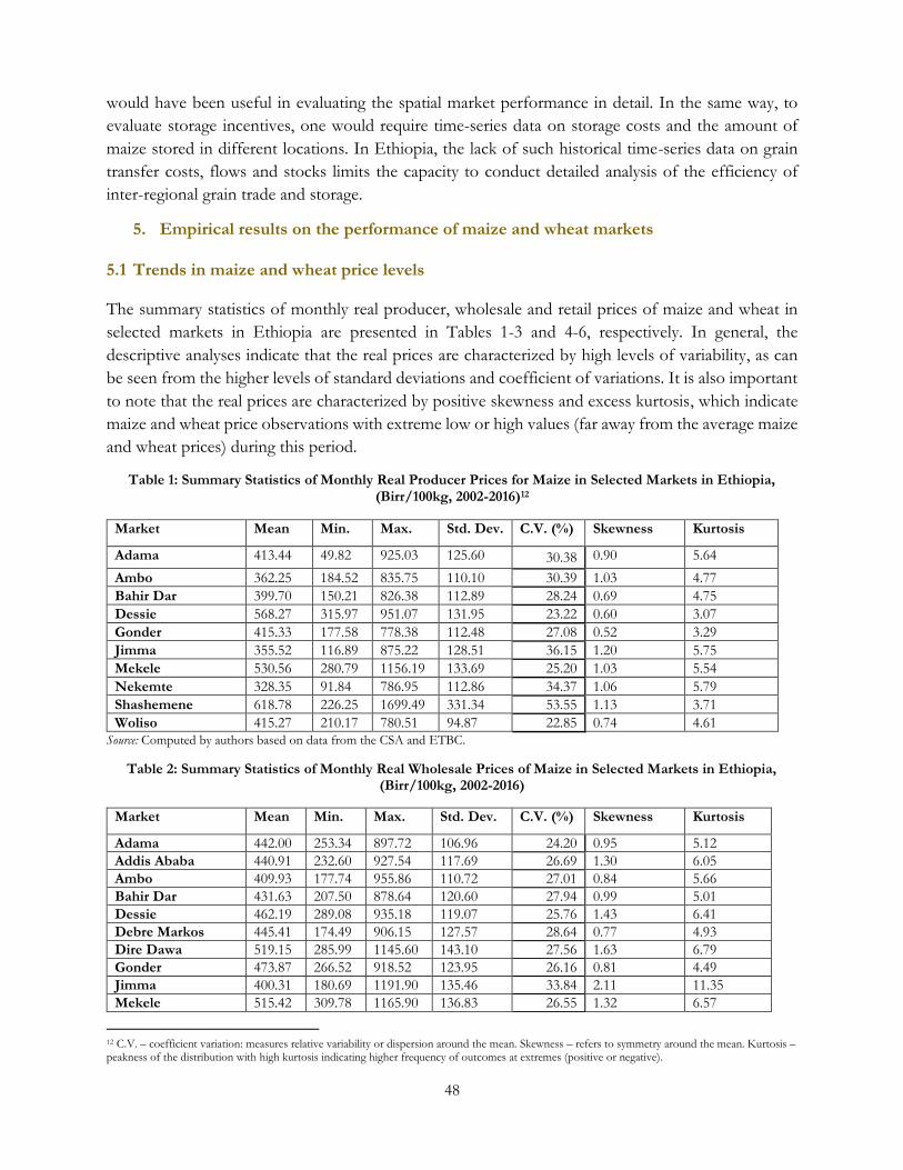
48

would have been useful in evaluating the spatial market performance in detail. In the same way, to

evaluate storage incentives, one would require time-series data on storage costs and the amount of

maize stored in different locations. In Ethiopia, the lack of such historical time-series data on grain

transfer costs, flows and stocks limits the capacity to conduct detailed analysis of the efficiency of

inter-regional grain trade and storage.

5. Empirical results on the performance of maize and wheat markets

5.1 Trends in maize and wheat price levels

The summary statistics of monthly real producer, wholesale and retail prices of maize and wheat in

selected markets in Ethiopia are presented in Tables 1-3 and 4-6, respectively. In general, the

descriptive analyses indicate that the real prices are characterized by high levels of variability, as can

be seen from the higher levels of standard deviations and coefficient of variations. It is also important

to note that the real prices are characterized by positive skewness and excess kurtosis, which indicate

maize and wheat price observations with extreme low or high values (far away from the average maize

and wheat prices) during this period.

Table 1: Summary Statistics of Monthly Real Producer Prices for Maize in Selected Markets in Ethiopia, (Birr/100kg, 2002-2016)12

Market Mean Min. Max. Std. Dev. C.V. (%) Skewness Kurtosis

Adama 413.44 49.82 925.03 125.60 30.38 0.90 5.64

Ambo 362.25 184.52 835.75 110.10 30.39 1.03 4.77

Bahir Dar 399.70 150.21 826.38 112.89 28.24 0.69 4.75

Dessie 568.27 315.97 951.07 131.95 23.22 0.60 3.07

Gonder 415.33 177.58 778.38 112.48 27.08 0.52 3.29

Jimma 355.52 116.89 875.22 128.51 36.15 1.20 5.75

Mekele 530.56 280.79 1156.19 133.69 25.20 1.03 5.54

Nekemte 328.35 91.84 786.95 112.86 34.37 1.06 5.79

Shashemene 618.78 226.25 1699.49 331.34 53.55 1.13 3.71

Woliso 415.27 210.17 780.51 94.87 22.85 0.74 4.61 Source: Computed by authors based on data from the CSA and ETBC.

Table 2: Summary Statistics of Monthly Real Wholesale Prices of Maize in Selected Markets in Ethiopia, (Birr/100kg, 2002-2016)


Adama 442.00 253.34 897.72 106.96 24.20 0.95 5.12

Addis Ababa 440.91 232.60 927.54 117.69 26.69 1.30 6.05

Ambo 409.93 177.74 955.86 110.72 27.01 0.84 5.66

Bahir Dar 431.63 207.50 878.64 120.60 27.94 0.99 5.01

Dessie 462.19 289.08 935.18 119.07 25.76 1.43 6.41

Debre Markos 445.41 174.49 906.15 127.57 28.64 0.77 4.93

Dire Dawa 519.15 285.99 1145.60 143.10 27.56 1.63 6.79

Gonder 473.87 266.52 918.52 123.95 26.16 0.81 4.49

Jimma 400.31 180.69 1191.90 135.46 33.84 2.11 11.35

Mekele 515.42 309.78 1165.90 136.83 26.55 1.32 6.57

12 C.V. – coefficient variation: measures relative variability or dispersion around the mean. Skewness – refers to symmetry around the mean. Kurtosis – peakness of the distribution with high kurtosis indicating higher frequency of outcomes at extremes (positive or negative).

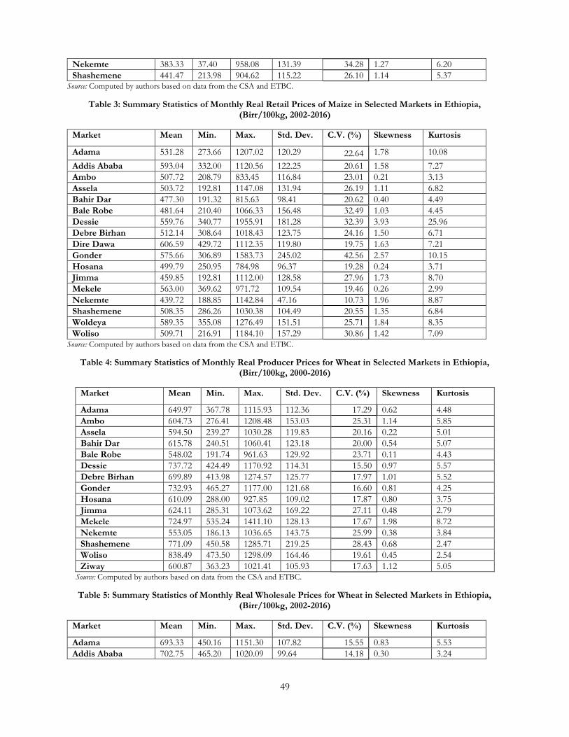
49

Nekemte 383.33 37.40 958.08 131.39 34.28 1.27 6.20

Shashemene 441.47 213.98 904.62 115.22 26.10 1.14 5.37 Source: Computed by authors based on data from the CSA and ETBC.

Table 3: Summary Statistics of Monthly Real Retail Prices of Maize in Selected Markets in Ethiopia, (Birr/100kg, 2002-2016)


Adama 531.28 273.66 1207.02 120.29 22.64 1.78 10.08

Addis Ababa 593.04 332.00 1120.56 122.25 20.61 1.58 7.27

Ambo 507.72 208.79 833.45 116.84 23.01 0.21 3.13

Assela 503.72 192.81 1147.08 131.94 26.19 1.11 6.82

Bahir Dar 477.30 191.32 815.63 98.41 20.62 0.40 4.49

Bale Robe 481.64 210.40 1066.33 156.48 32.49 1.03 4.45

Dessie 559.76 340.77 1955.91 181.28 32.39 3.93 25.96

Debre Birhan 512.14 308.64 1018.43 123.75 24.16 1.50 6.71

Dire Dawa 606.59 429.72 1112.35 119.80 19.75 1.63 7.21

Gonder 575.66 306.89 1583.73 245.02 42.56 2.57 10.15

Hosana 499.79 250.95 784.98 96.37 19.28 0.24 3.71

Jimma 459.85 192.81 1112.00 128.58 27.96 1.73 8.70

Mekele 563.00 369.62 971.72 109.54 19.46 0.26 2.99

Nekemte 439.72 188.85 1142.84 47.16 10.73 1.96 8.87

Shashemene 508.35 286.26 1030.38 104.49 20.55 1.35 6.84

Woldeya 589.35 355.08 1276.49 151.51 25.71 1.84 8.35


Table 4: Summary Statistics of Monthly Real Producer Prices for Wheat in Selected Markets in Ethiopia, (Birr/100kg, 2000-2016)


Adama 649.97 367.78 1115.93 112.36 17.29 0.62 4.48

Ambo 604.73 276.41 1208.48 153.03 25.31 1.14 5.85

Assela 594.50 239.27 1030.28 119.83 20.16 0.22 5.01

Bahir Dar 615.78 240.51 1060.41 123.18 20.00 0.54 5.07

Bale Robe 548.02 191.74 961.63 129.92 23.71 0.11 4.43

Dessie 737.72 424.49 1170.92 114.31 15.50 0.97 5.57

Debre Birhan 699.89 413.98 1274.57 125.77 17.97 1.01 5.52

Gonder 732.93 465.27 1177.00 121.68 16.60 0.81 4.25

Hosana 610.09 288.00 927.85 109.02 17.87 0.80 3.75

Jimma 624.11 285.31 1073.62 169.22 27.11 0.48 2.79

Mekele 724.97 535.24 1411.10 128.13 17.67 1.98 8.72

Nekemte 553.05 186.13 1036.65 143.75 25.99 0.38 3.84

Shashemene 771.09 450.58 1285.71 219.25 28.43 0.68 2.47

Woliso 838.49 473.50 1298.09 164.46 19.61 0.45 2.54

Ziway 600.87 363.23 1021.41 105.93 17.63 1.12 5.05 Source: Computed by authors based on data from the CSA and ETBC.

Table 5: Summary Statistics of Monthly Real Wholesale Prices for Wheat in Selected Markets in Ethiopia, (Birr/100kg, 2002-2016)


Adama 693.33 450.16 1151.30 107.82 15.55 0.83 5.53

Addis Ababa 702.75 465.20 1020.09 99.64 14.18 0.30 3.24

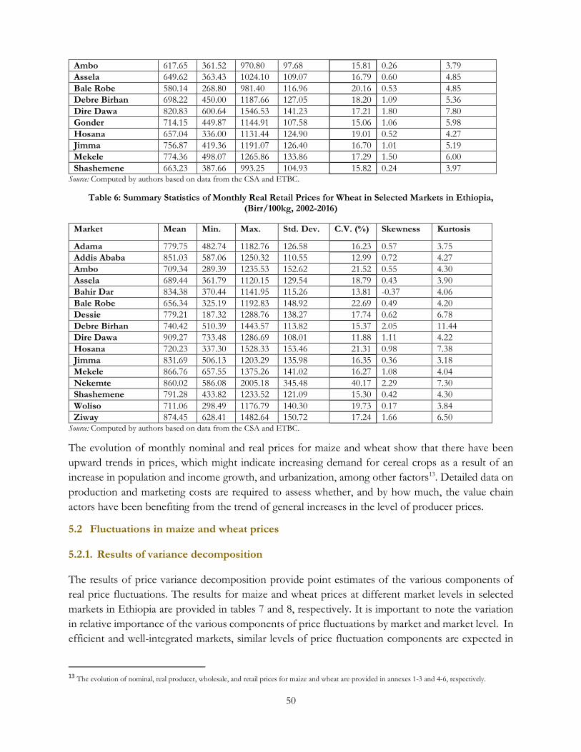
50

Ambo 617.65 361.52 970.80 97.68 15.81 0.26 3.79

Assela 649.62 363.43 1024.10 109.07 16.79 0.60 4.85

Bale Robe 580.14 268.80 981.40 116.96 20.16 0.53 4.85

Debre Birhan 698.22 450.00 1187.66 127.05 18.20 1.09 5.36

Dire Dawa 820.83 600.64 1546.53 141.23 17.21 1.80 7.80

Gonder 714.15 449.87 1144.91 107.58 15.06 1.06 5.98

Hosana 657.04 336.00 1131.44 124.90 19.01 0.52 4.27

Jimma 756.87 419.36 1191.07 126.40 16.70 1.01 5.19

Mekele 774.36 498.07 1265.86 133.86 17.29 1.50 6.00


Table 6: Summary Statistics of Monthly Real Retail Prices for Wheat in Selected Markets in Ethiopia, (Birr/100kg, 2002-2016)


Adama 779.75 482.74 1182.76 126.58 16.23 0.57 3.75

Addis Ababa 851.03 587.06 1250.32 110.55 12.99 0.72 4.27

Ambo 709.34 289.39 1235.53 152.62 21.52 0.55 4.30

Assela 689.44 361.79 1120.15 129.54 18.79 0.43 3.90

Bahir Dar 834.38 370.44 1141.95 115.26 13.81 -0.37 4.06

Bale Robe 656.34 325.19 1192.83 148.92 22.69 0.49 4.20

Dessie 779.21 187.32 1288.76 138.27 17.74 0.62 6.78

Debre Birhan 740.42 510.39 1443.57 113.82 15.37 2.05 11.44

Dire Dawa 909.27 733.48 1286.69 108.01 11.88 1.11 4.22

Hosana 720.23 337.30 1528.33 153.46 21.31 0.98 7.38

Jimma 831.69 506.13 1203.29 135.98 16.35 0.36 3.18

Mekele 866.76 657.55 1375.26 141.02 16.27 1.08 4.04

Nekemte 860.02 586.08 2005.18 345.48 40.17 2.29 7.30

Shashemene 791.28 433.82 1233.52 121.09 15.30 0.42 4.30

Woliso 711.06 298.49 1176.79 140.30 19.73 0.17 3.84

Ziway 874.45 628.41 1482.64 150.72 17.24 1.66 6.50 Source: Computed by authors based on data from the CSA and ETBC.

The evolution of monthly nominal and real prices for maize and wheat show that there have been

upward trends in prices, which might indicate increasing demand for cereal crops as a result of an

increase in population and income growth, and urbanization, among other factors13. Detailed data on

production and marketing costs are required to assess whether, and by how much, the value chain

actors have been benefiting from the trend of general increases in the level of producer prices.

5.2 Fluctuations in maize and wheat prices

5.2.1. Results of variance decomposition

The results of price variance decomposition provide point estimates of the various components of

real price fluctuations. The results for maize and wheat prices at different market levels in selected

markets in Ethiopia are provided in tables 7 and 8, respectively. It is important to note the variation

in relative importance of the various components of price fluctuations by market and market level. In

efficient and well-integrated markets, similar levels of price fluctuation components are expected in

13 The evolution of nominal, real producer, wholesale, and retail prices for maize and wheat are provided in annexes 1-3 and 4-6, respectively.

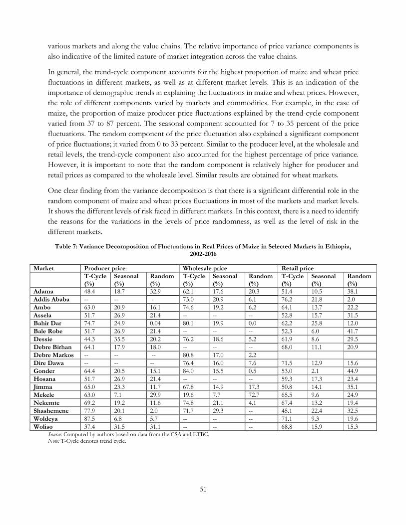
51

various markets and along the value chains. The relative importance of price variance components is

also indicative of the limited nature of market integration across the value chains.

In general, the trend-cycle component accounts for the highest proportion of maize and wheat price

fluctuations in different markets, as well as at different market levels. This is an indication of the

importance of demographic trends in explaining the fluctuations in maize and wheat prices. However,

the role of different components varied by markets and commodities. For example, in the case of

maize, the proportion of maize producer price fluctuations explained by the trend-cycle component

varied from 37 to 87 percent. The seasonal component accounted for 7 to 35 percent of the price

fluctuations. The random component of the price fluctuation also explained a significant component

of price fluctuations; it varied from 0 to 33 percent. Similar to the producer level, at the wholesale and

retail levels, the trend-cycle component also accounted for the highest percentage of price variance.

However, it is important to note that the random component is relatively higher for producer and

retail prices as compared to the wholesale level. Similar results are obtained for wheat markets.

One clear finding from the variance decomposition is that there is a significant differential role in the

random component of maize and wheat prices fluctuations in most of the markets and market levels.

It shows the different levels of risk faced in different markets. In this context, there is a need to identify

the reasons for the variations in the levels of price randomness, as well as the level of risk in the

different markets.

Table 7: Variance Decomposition of Fluctuations in Real Prices of Maize in Selected Markets in Ethiopia, 2002-2016

Market Producer price Wholesale price Retail price

T-Cycle (%)

Seasonal (%)

Random (%)

T-Cycle (%)

Seasonal (%)

Random (%)

T-Cycle (%)

Seasonal (%)

Random (%)

Adama 48.4 18.7 32.9 62.1 17.6 20.3 51.4 10.5 38.1

Addis Ababa -- -- - 73.0 20.9 6.1 76.2 21.8 2.0

Ambo 63.0 20.9 16.1 74.6 19.2 6.2 64.1 13.7 22.2

Assela 51.7 26.9 21.4 -- -- -- 52.8 15.7 31.5

Bahir Dar 74.7 24.9 0.04 80.1 19.9 0.0 62.2 25.8 12.0

Bale Robe 51.7 26.9 21.4 -- -- -- 52.3 6.0 41.7

Dessie 44.3 35.5 20.2 76.2 18.6 5.2 61.9 8.6 29.5

Debre Birhan 64.1 17.9 18.0 -- -- -- 68.0 11.1 20.9

Debre Markos -- -- -- 80.8 17.0 2.2

Dire Dawa -- -- -- 76.4 16.0 7.6 71.5 12.9 15.6

Gonder 64.4 20.5 15.1 84.0 15.5 0.5 53.0 2.1 44.9

Hosana 51.7 26.9 21.4 -- -- -- 59.3 17.3 23.4

Jimma 65.0 23.3 11.7 67.8 14.9 17.3 50.8 14.1 35.1

Mekele 63.0 7.1 29.9 19.6 7.7 72.7 65.5 9.6 24.9

Nekemte 69.2 19.2 11.6 74.8 21.1 4.1 67.4 13.2 19.4

Shashemene 77.9 20.1 2.0 71.7 29.3 -- 45.1 22.4 32.5

Woldeya 87.5 6.8 5.7 -- -- -- 71.1 9.3 19.6

Woliso 37.4 31.5 31.1 -- -- -- 68.8 15.9 15.3 Source: Computed by authors based on data from the CSA and ETBC. Note: T-Cycle denotes trend cycle.

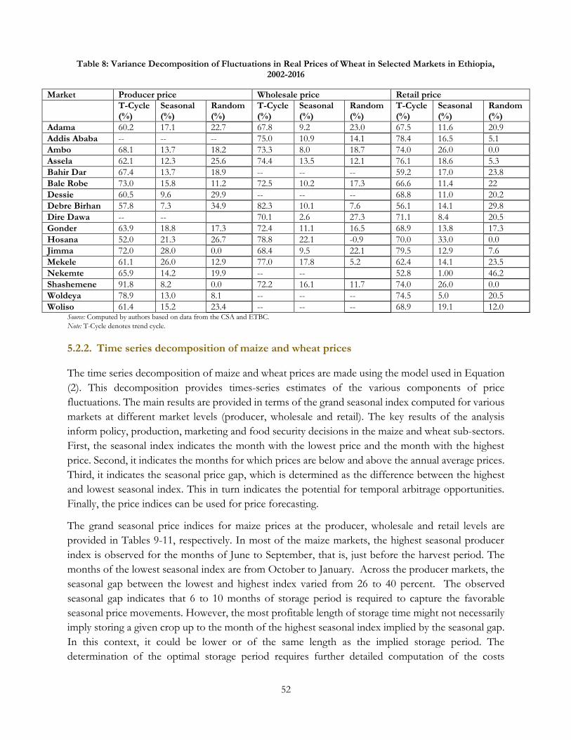
52

Table 8: Variance Decomposition of Fluctuations in Real Prices of Wheat in Selected Markets in Ethiopia, 2002-2016

Market Producer price Wholesale price Retail price

T-Cycle (%)

Seasonal (%)

Random (%)

T-Cycle (%)

Seasonal (%)

Random (%)

T-Cycle (%)

Seasonal (%)

Random (%)

Adama 60.2 17.1 22.7 67.8 9.2 23.0 67.5 11.6 20.9

Addis Ababa -- -- -- 75.0 10.9 14.1 78.4 16.5 5.1

Ambo 68.1 13.7 18.2 73.3 8.0 18.7 74.0 26.0 0.0

Assela 62.1 12.3 25.6 74.4 13.5 12.1 76.1 18.6 5.3

Bahir Dar 67.4 13.7 18.9 -- -- -- 59.2 17.0 23.8

Bale Robe 73.0 15.8 11.2 72.5 10.2 17.3 66.6 11.4 22

Dessie 60.5 9.6 29.9 -- -- -- 68.8 11.0 20.2

Debre Birhan 57.8 7.3 34.9 82.3 10.1 7.6 56.1 14.1 29.8

Dire Dawa -- -- 70.1 2.6 27.3 71.1 8.4 20.5

Gonder 63.9 18.8 17.3 72.4 11.1 16.5 68.9 13.8 17.3

Hosana 52.0 21.3 26.7 78.8 22.1 -0.9 70.0 33.0 0.0

Jimma 72.0 28.0 0.0 68.4 9.5 22.1 79.5 12.9 7.6

Mekele 61.1 26.0 12.9 77.0 17.8 5.2 62.4 14.1 23.5

Nekemte 65.9 14.2 19.9 -- -- 52.8 1.00 46.2

Shashemene 91.8 8.2 0.0 72.2 16.1 11.7 74.0 26.0 0.0

Woldeya 78.9 13.0 8.1 -- -- -- 74.5 5.0 20.5

Woliso 61.4 15.2 23.4 -- -- -- 68.9 19.1 12.0 Source: Computed by authors based on data from the CSA and ETBC.

Note: T-Cycle denotes trend cycle.

5.2.2. Time series decomposition of maize and wheat prices

The time series decomposition of maize and wheat prices are made using the model used in Equation

(2). This decomposition provides times-series estimates of the various components of price

fluctuations. The main results are provided in terms of the grand seasonal index computed for various

markets at different market levels (producer, wholesale and retail). The key results of the analysis

inform policy, production, marketing and food security decisions in the maize and wheat sub-sectors.

First, the seasonal index indicates the month with the lowest price and the month with the highest

price. Second, it indicates the months for which prices are below and above the annual average prices.

Third, it indicates the seasonal price gap, which is determined as the difference between the highest

and lowest seasonal index. This in turn indicates the potential for temporal arbitrage opportunities.

Finally, the price indices can be used for price forecasting.

The grand seasonal price indices for maize prices at the producer, wholesale and retail levels are

provided in Tables 9-11, respectively. In most of the maize markets, the highest seasonal producer

index is observed for the months of June to September, that is, just before the harvest period. The

months of the lowest seasonal index are from October to January. Across the producer markets, the

seasonal gap between the lowest and highest index varied from 26 to 40 percent. The observed

seasonal gap indicates that 6 to 10 months of storage period is required to capture the favorable

seasonal price movements. However, the most profitable length of storage time might not necessarily

imply storing a given crop up to the month of the highest seasonal index implied by the seasonal gap.

In this context, it could be lower or of the same length as the implied storage period. The

determination of the optimal storage period requires further detailed computation of the costs

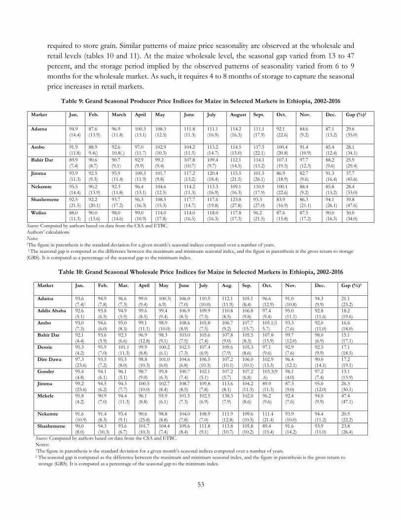
53

required to store grain. Similar patterns of maize price seasonality are observed at the wholesale and

retail levels (tables 10 and 11). At the maize wholesale level, the seasonal gap varied from 13 to 47

percent, and the storage period implied by the observed patterns of seasonality varied from 6 to 9

months for the wholesale market. As such, it requires 4 to 8 months of storage to capture the seasonal

price increases in retail markets.

Table 9: Grand Seasonal Producer Price Indices for Maize in Selected Markets in Ethiopia, 2002-2016

Market Jan. Feb. March April May June July August Sept. Oct. Nov. Dec. Gap (%)2

Adama 94.9 (14.4)1

87.6 (13.9)

96.9 (11.8)

100.3 (13.1)

108.3 (12.5)

111.8 (11.3)

111.1 (16.9)

114.2 (16.3)

111.1 (17.9)

92.1 (22.6)

84.6 (9.2)

87.1 (13.2)

29.6 (35.0)

Ambo 91.9 (11.8)

88.9 9.4()

92.6 10.8(.)

97.0 (11.7)

102.9 (10.3)

104.2 (11.5)

113.2 (14.7)

114.5 (15.0)

117.5 (22.1)

100.4 (20.8)

91.4 (10.9)

85.4 (12.4)

28.1 (34.1)

Bahir Dar 89.9 (7.4)

90.6 (8.7)

90.7 (9.1)

92.9 (9.9)

99.2 (9.4)

107.8 (10.7)

109.4 (9.7)

112.1 (14.5)

114.1 (13.2)

107.1 (19.5)

97.7 (12.3)

88.2 (9.6)

25.9 (29.4)

Jimma 93.9 (11.3)

92.5 (9.3)

95.9 (11.4)

100.3 (11.9)

101.7 (9.8)

117.2 (13.2)

120.4 (18.4)

115.5 (21.5)

101.5 (26.1)

86.9 (18.9)

82.7 (9.6)

91.3 (16.4)

37.7 (45.6)

Nekemte 95.5 (14.4)

90.2 (13.9)

92.3 (11.8)

96.4 (13.1)

104.6 (12.5)

114.2 (11.3)

113.3 (16.9)

109.1 (16.3)

110.9 (17.9)

100.1 (22.6)

88.4 (9.2)

85.8 (13.2)

28.4 (33.0)

Shashemene 92.5 (21.5)

92.2 (20.1)

93.7 (17.2)

96.3 (16.3)

108.5 (15.3)

117.7 (14.7)

117.6 (19.8)

123.8 (27.8)

93.3 (27.0)

83.9 (16.9)

86.3 (21.1)

94.1 (26.1)

39.8 (47.6)

Woliso 88.0 (11.3)

90.0 (13.6)

98.0 (14.6)

99.0 (10.9)

114.0 (17.8)

114.0 (16.5)

118.0 (16.3)

117.8 (17.3)

96.2 (21.5)

87.6 (15.8)

87.5 (17.2)

90.0 (16.3)

30.0 (34.0)

Source: Computed by authors based on data from the CSA and ETBC.

Authors’ calculations

Notes: 1The figure in parenthesis is the standard deviation for a given month’s seasonal indices computed over a number of years.

2 The seasonal gap is computed as the difference between the maximum and minimum seasonal index, and the figure in parenthesis is the gross return to storage

(GRS). It is computed as a percentage of the seasonal gap to the minimum index.

Table 10: Grand Seasonal Wholesale Price Indices for Maize in Selected Markets in Ethiopia, 2002-2016

Market Jan. Feb. Mar. April May June July Aug. Sep. Oct. Nov. Dec. Gap (%)2

Adama 93.6 (7.4)1

94.9 (7.8)

96.6 (7.3)

99.0 (9.4)

100.3(6.9)

106.0 (7.0)

110.5 (10.0)

112.1 (11.9)

105.1 (8.4)

96.6 (12.9)

91.0 (10.8)

94.3 (9.9)

21.1 (23.2)

Addis Ababa 92.6 (5.1)

93.8 (6.5)

94.9 (5.5)

99.6 (8.5)

99.4 (9.4)

106.9 (8.3)

109.9 (7.5)

110.8 (8.5)

106.8 (9.8)

97.4 (9.4)

95.0 (11.1)

92.8 (11.6)

18.2 (19.6)

Ambo 93.0 (7.3)

94.6 (6.0)

95.0 (8.3)

99.1 (11.1)

98.9 (10.0)

108.6 (8.9)

105.8 (7.5)

106.7 (9.2)

107.7 (15.7)

105.1(15.7)

93.3 (7.6)

92.0 (11.0)

16.6 (18.0)


93.6 (5.9)

92.3 (6.6)

96.9 (12.8)

98.3 (9.1)

103.0 (7.5)

105.6 (7.4)

107.8 (9.0)

105.5 (8.3)

107.8 (15.9)

99.7 (12.0)

98.0 (6.9)

15.1 (17.1)

Dessie 95.3 (4.2)

95.9 (7.0)

101.1 (11.3)

99.9 (8.8)

100.2 (6.1)

102.5 (7.3)

107.4 (6.9)

109.6 (7.9)

105.3 (8.6)

97.1 (9.6)

92.9 (7.6)

92.5 (9.9)

17.1 (18.5)

Dire Dawa 97.3 (23.6)

93.5 (7.2)

95.5 (8.0)

98.8 (10.3)

101.0 (6.0)

104.6 (6.8)

106.5 (10.3)

107.2 (10.1)

106.0 (10.1)

102.9 (13.3)

96.4 (12.1)

90.0 (14.1)

17.2 (19.1)

Gonder 95.4 (4.8)

94.1 (6.1)

96.1 (5.1)

98.7 (9.0)

99.8 (6.3)

100.7 (7.4)

102.1 (5.1)

107.2 (5.7)

107.2 (6.8)

103.3(9.6)

98.1 (4.0)

97.2 (7.4)

13.1 (13.9)

Jimma 99.2 (23.6)

94.5 (6.2)

94.3 (7.7)

100.5 (10.0)

102.7 (8.4)

108.7 (8.5)

109.8 (7.8)

113.6 (8.1)

104.2 (11.5)

89.9 (11.3)

87.3 (9.0)

95.0 (12.0)

26.3 (30.1)

Mekele 95.8 (4.2)

90.9 (7.0)

94.4 (11.3)

96.1 (8.8)

95.9 (6.1)

101.5 (7.3)

102.5 (6.9)

138.3 (7.9)

102.0 (8.6)

96.2 (9.6)

92.4 (7.6)

94.0 (9.9)

47.4 (47.1)

Nekemte 91.6 (10.9)

91.4 (8.3)

93.4 (9.1)

90.6 (25.8)

98.8 (8.8)

104.0 (7.8)

108.9 (7.0)

111.9 (12.8)

109.6 (10.5)

111.4 (21.4)

93.9 (10.0)

94.4 (11.2)

20.5 (22.2)


94.3 (10.3)

93.6 (6.7)

101.7 (10.3)

104.4 (7.4)

109.6 (8.4)

111.8 (9.1)

113.8 (10.7)

105.8 (10.2)

89.4 (15.4)

91.6 (14.2)

93.9 (11.0)

23.8 (26.4)


Notes: 1The figure in parenthesis is the standard deviation for a given month’s seasonal indices computed over a number of years. 2 The seasonal gap is computed as the difference between the maximum and minimum seasonal index, and the figure in parenthesis is the gross return to

storage (GRS). It is computed as a percentage of the seasonal gap to the minimum index.

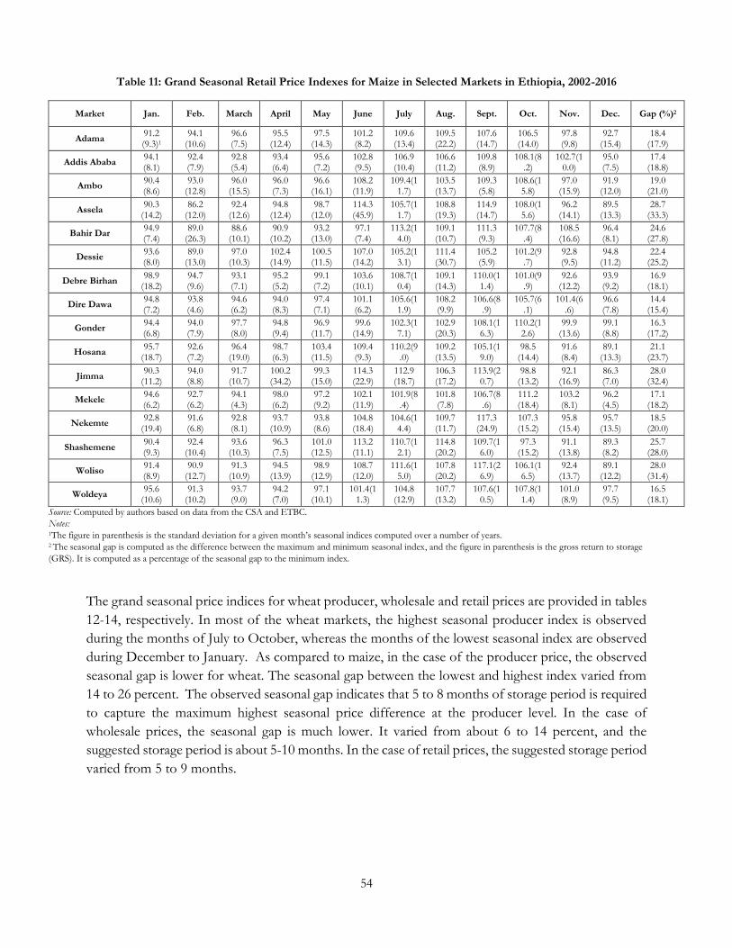
54

Table 11: Grand Seasonal Retail Price Indexes for Maize in Selected Markets in Ethiopia, 2002-2016

Market Jan. Feb. March April May June July Aug. Sept. Oct. Nov. Dec. Gap (%)2

Adama 91.2 (9.3)1

94.1 (10.6)

96.6 (7.5)

95.5 (12.4)

97.5 (14.3)

101.2 (8.2)

109.6 (13.4)

109.5 (22.2)

107.6 (14.7)

106.5 (14.0)

97.8 (9.8)

92.7 (15.4)

18.4 (17.9)


92.4 (7.9)

92.8 (5.4)

93.4 (6.4)

95.6 (7.2)

102.8 (9.5)

106.9 (10.4)

106.6 (11.2)

109.8 (8.9)

108.1(8.2)

102.7(10.0)

95.0 (7.5)

17.4 (18.8)

Ambo 90.4 (8.6)

93.0 (12.8)

96.0 (15.5)

96.0 (7.3)

96.6 (16.1)

108.2 (11.9)

109.4(11.7)

103.5 (13.7)

109.3 (5.8)

108.6(15.8)

97.0 (15.9)

91.9 (12.0)

19.0 (21.0)

Assela 90.3

(14.2) 86.2

(12.0) 92.4

(12.6) 94.8

(12.4) 98.7

(12.0) 114.3 (45.9)

105.7(11.7)

108.8 (19.3)

114.9 (14.7)

108.0(15.6)

96.2 (14.1)

89.5 (13.3)

28.7 (33.3)


89.0 (26.3)

88.6 (10.1)

90.9 (10.2)

93.2 (13.0)

97.1 (7.4)

113.2(14.0)

109.1 (10.7)

111.3 (9.3)

107.7(8.4)

108.5 (16.6)

96.4 (8.1)

24.6 (27.8)

Dessie 93.6 (8.0)

89.0 (13.0)

97.0 (10.3)

102.4 (14.9)

100.5 (11.5)

107.0 (14.2)

105.2(13.1)

111.4 (30.7)

105.2 (5.9)

101.2(9.7)

92.8 (9.5)

94.8 (11.2)

22.4 (25.2)

Debre Birhan 98.9

(18.2) 94.7 (9.6)

93.1 (7.1)

95.2 (5.2)

99.1 (7.2)

103.6 (10.1)

108.7(10.4)

109.1 (14.3)

110.0(11.4)

101.0(9.9)

92.6 (12.2)

93.9 (9.2)

16.9 (18.1)

Dire Dawa 94.8 (7.2)

93.8 (4.6)

94.6 (6.2)

94.0 (8.3)

97.4 (7.1)

101.1 (6.2)

105.6(11.9)

108.2 (9.9)

106.6(8.9)

105.7(6.1)

101.4(6.6)

96.6 (7.8)

14.4 (15.4)

Gonder 94.4 (6.8)

94.0 (7.9)

97.7 (8.0)

94.8 (9.4)

96.9 (11.7)

99.6 (14.9)

102.3(17.1)

102.9 (20.3)

108.1(16.3)

110.2(12.6)

99.9 (13.6)

99.1 (8.8)

16.3 (17.2)

Hosana 95.7

(18.7) 92.6 (7.2)

96.4 (19.0)

98.7 (6.3)

103.4 (11.5)

109.4 (9.3)

110.2(9.0)

109.2 (13.5)

105.1(19.0)

98.5 (14.4)

91.6 (8.4)

89.1 (13.3)

21.1 (23.7)

Jimma 90.3

(11.2) 94.0 (8.8)

91.7 (10.7)

100.2 (34.2)

99.3 (15.0)

114.3 (22.9)

112.9 (18.7)

106.3 (17.2)

113.9(20.7)

98.8 (13.2)

92.1 (16.9)

86.3 (7.0)

28.0 (32.4)

Mekele 94.6 (6.2)

92.7 (6.2)

94.1 (4.3)

98.0 (6.2)

97.2 (9.2)

102.1 (11.9)

101.9(8.4)

101.8 (7.8)

106.7(8.6)

111.2 (18.4)

103.2 (8.1)

96.2 (4.5)

17.1 (18.2)

Nekemte 92.8

(19.4) 91.6 (6.8)

92.8 (8.1)

93.7 (10.9)

93.8 (8.6)

104.8 (18.4)

104.6(14.4)

109.7 (11.7)

117.3 (24.9)

107.3 (15.2)

95.8 (15.4)

95.7 (13.5)

18.5 (20.0)


92.4 (10.4)

93.6 (10.3)

96.3 (7.5)

101.0 (12.5)

113.2 (11.1)

110.7(12.1)

114.8 (20.2)

109.7(16.0)

97.3 (15.2)

91.1 (13.8)

89.3 (8.2)

25.7 (28.0)

Woliso 91.4 (8.9)

90.9 (12.7)

91.3 (10.9)

94.5 (13.9)

98.9 (12.9)

108.7 (12.0)

111.6(15.0)

107.8 (20.2)

117.1(26.9)

106.1(16.5)

92.4 (13.7)

89.1 (12.2)

28.0 (31.4)

Woldeya 95.6

(10.6) 91.3

(10.2) 93.7 (9.0)

94.2 (7.0)

97.1 (10.1)

101.4(11.3)

104.8 (12.9)

107.7 (13.2)

107.6(10.5)

107.8(11.4)

101.0 (8.9)

97.7 (9.5)

16.5 (18.1)


Notes:

1The figure in parenthesis is the standard deviation for a given month’s seasonal indices computed over a number of years. 2 The seasonal gap is computed as the difference between the maximum and minimum seasonal index, and the figure in parenthesis is the gross return to storage


The grand seasonal price indices for wheat producer, wholesale and retail prices are provided in tables

12-14, respectively. In most of the wheat markets, the highest seasonal producer index is observed

during the months of July to October, whereas the months of the lowest seasonal index are observed

during December to January. As compared to maize, in the case of the producer price, the observed

seasonal gap is lower for wheat. The seasonal gap between the lowest and highest index varied from

14 to 26 percent. The observed seasonal gap indicates that 5 to 8 months of storage period is required

to capture the maximum highest seasonal price difference at the producer level. In the case of

wholesale prices, the seasonal gap is much lower. It varied from about 6 to 14 percent, and the

suggested storage period is about 5-10 months. In the case of retail prices, the suggested storage period

varied from 5 to 9 months.

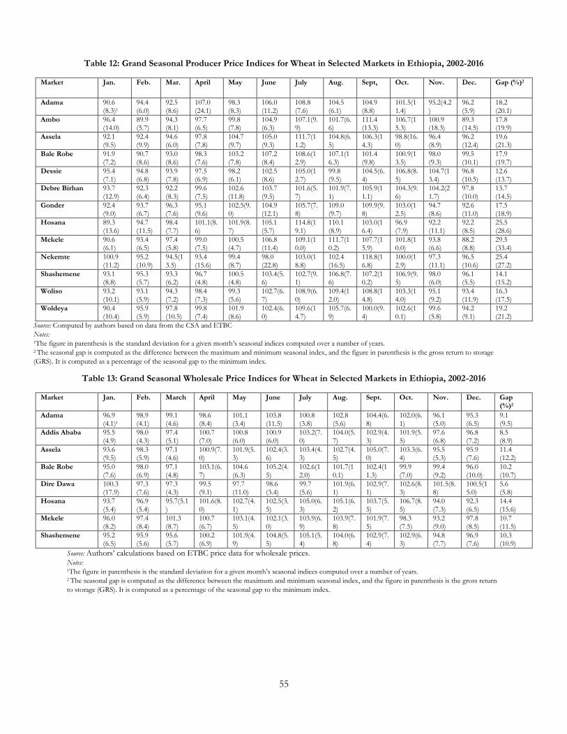
55

Table 12: Grand Seasonal Producer Price Indices for Wheat in Selected Markets in Ethiopia, 2002-2016

Market Jan. Feb. Mar. April May June July Aug. Sept, Oct. Nov. Dec. Gap (%)2

Adama 90.6 (8.3)1

94.4 (6.0)

92.5 (8.6)

107.0 (24.1)

98.3 (8.3)

106.0 (11.2)

108.8 (7.6)

104.5 (6.1)

104.9 (8.8)

101.5(11.4)

95.2(4.2)

96.2 (5.9)

18.2 (20.1)

Ambo 96.4 (14.0)

89.9 (5.7)

94.3 (8.1)

97.7 (6.5)

99.8 (7.8)

104.9 (6.3)

107.1(9.9)

101.7(6.6)

111.4 (13.3)

106.7(15.3)

100.9 (18.3)

89.3 (14.5)

17.8 (19.9)

Assela 92.1 (9.5)

92.4 (9.9)

94.6 (6.0)

97.8 (7.8)

104.7 (9.7)

105.0 (9.3)

111.7(11.2)

104.8(6.5)

106.3(14.3)

98.8(16.0)

96.4 (8.9)

96.2 (12.4)

19.6 (21.3)

Bale Robe 91.9 (7.2)

90.7 (8.6)

93.0 (8.6)

98.3 (7.6)

103.2 (7.8)

107.2 (8.4)

108.6(12.9)

107.1(16.3)

101.4 (9.8)

100.9(13.5)

98.0 (9.3)

99.5 (10.1)

17.9 (19.7)

Dessie 95.4 (7.1)

94.8 (6.8)

93.9 (7.8)

97.5 (6.9)

98.2 (6.1)

102.5 (8.6)

105.0(12.7)

99.8 (9.5)

104.5(6.4)

106.8(8.5)

104.7(13.4)

96.8 (10.5)

12.6 (13.7)

Debre Birhan 93.7 (12.9)

92.3 (6.4)

92.2 (8.3)

99.6 (7.5)

102.6 (11.8)

103.7 (9.5)

101.6(5.7)

101.9(7.1)

105.9(11.1)

104.3(9.6)

104.2(21.7)

97.8 (10.0)

13.7 (14.5)

Gonder 92.4 (9.0)

93.7 (6.7)

96.3 (7.6)

95.1 (9.6)

102.5(9.0)

104.9 (12.1)

105.7(7.8)

109.0 (9.7)

109.9(9.8)

103.0(12.5)

94.7 (8.6)

92.6 (11.0)

17.5 (18.9)

Hosana 89.3 (13.6)

94.7 (11.5)

98.4 (7.7)

101.1(8.6)

101.9(8.7)

105.1 (5.7)

114.8(19.1)

110.1 (8.9)

103.0(16.4)

96.9 (7.9)

92.2 (11.1)

92.2 (8.5)

25.5 (28.6)

Mekele 90.6 (6.1)

93.4 (6.5)

97.4 (5.8)

99.0 (7.5)

100.5 (4.7)

106.8 (11.4)

109.1(10.0)

111.7(10.2)

107.7(15.9)

101.8(10.0)

93.8 (6.6)

88.2 (8.8)

29.5 (33.4)

Nekemte 100.9 (11.2)

95.2 (10.9)

94.5(13.5)

93.4 (15.6)

99.4 (8.7)

98.0 (22.8)

103.0(18.8)

102.4 (16.5)

118.8(16.8)

100.0(12.9)

97.3 (11.1)

96.5 (10.6)

25.4 (27.2)


95.3 (5.7)

93.3 (6.2)

96.7 (4.8)

100.5 (4.8)

103.4(5.6)

102.7(9.1)

106.8(7.6)

107.2(10.2)

106.9(9.5)

98.0 (6.0)

96.1 (5.5)

14.1 (15.2)

Woliso 93.2 (10.1)

93.1 (5.9)

94.3 (7.2)

98.4 (7.3)

99.3 (5.6)

102.7(6.7)

108.9(6.0)

109.4(12.0)

108.8(14.8)

103.3(14.0)

95.1 (9.2)

93.4 (11.9)

16.3 (17.5)

Woldeya 90.4 (10.4)

95.9 (5.9)

97.8 (10.5)

99.8 (7.4)

101.9 (8.6)

102.4(6.0)

109.6(14.7)

105.7(6.9)

100.0(9.4)

102.6(10.1)

99.6 (5.8)

94.2 (9.1)

19.2 (21.2)

Source: Computed by authors based on data from the CSA and ETBC

Notes: 1The figure in parenthesis is the standard deviation for a given month’s seasonal indices computed over a number of years. 2 The seasonal gap is computed as the difference between the maximum and minimum seasonal index, and the figure in parenthesis is the gross return to storage


Table 13: Grand Seasonal Wholesale Price Indices for Wheat in Selected Markets in Ethiopia, 2002-2016


Adama 96.9 (4.1)1

98.9 (4.1)

99.1 (4.6)

98.6 (8.4)

101.1 (3.4)

103.8 (11.5)

100.8 (3.8)

102.8 (5.6)

104.4(6.8)

102.0(6.1)

96.1 (5.0)

95.3 (6.5)

9.1 (9.5)


98.0 (4.3)

97.4 (5.1)

100.7 (7.0)

100.8 (6.0)

100.9 (6.0)

103.2(7.0)

104.0(5.7)

102.9(4.3)

101.9(5.5)

97.6 (6.8)

96.8 (7.2)

8.5 (8.9)

Assela 93.6 (9.5)

98.3 (5.9)

97.1 (4.6)

100.9(7.0)

101.9(5.3)

102.4(3.6)

103.4(4.3)

102.7(4.5)

105.0(7.0)

103.3(6.4)

95.5 (5.3)

95.9 (7.6)

11.4 (12.2)


98.0 (6.9)

97.1 (4.8)

103.1(6.7)

104.6 (6.3)

105.2(4.5)

102.6(12.0)

101.7(10.1)

102.4(11.3)

99.9 (7.0)

99.4 (9.2)

96.0 (10.0)

10.2 (10.7)

Dire Dawa 100.3 (17.9)

97.3 (7.6)

97.3 (4.3)

99.5 (9.1)

97.7 (11.0)

98.6 (3.4)

99.7 (5.6)

101.9(6.1)

102.9(7.1)

102.6(8.3)

101.5(8.8)

100.5(15.0)

5.6 (5.8)

Hosana 93.7 (5.4)

96.9 (5.4)

95.7(5.1)

101.6(8.0)

102.7(4.1)

102.5(3.5)

105.0(6.3)

105.1(6.2)

103.7(5.5)

106.7(8.5)

94.0 (7.3)

92.3 (6.5)

14.4 (15.6)

Mekele 96.0 (8.2)

97.4 (8.4)

101.3 (8.7)

100.7 (6.7)

103.1(4.5)

102.1(3.0)

103.9(6.9)

103.9(7.8)

101.9(7.5)

98.3 (7.5)

93.2 (9.0)

97.8 (8.5)

10.7 (11.5)


95.9 (5.6)

95.6 (5.7)

100.2 (6.9)

101.9(4.9)

104.8(5.5)

105.1(5.4)

104.0(6.8)

102.9(7.4)

102.9(6.3)

94.8 (7.7)

96.9 (7.6)

10.3 (10.9)

Source: Authors’ calculations based on ETBC price data for wholesale prices. Notes: 1The figure in parenthesis is the standard deviation for a given month’s seasonal indices computed over a number of years. 2 The seasonal gap is computed as the difference between the maximum and minimum seasonal index, and the figure in parenthesis is the gross return

to storage (GRS). It is computed as a percentage of the seasonal gap to the minimum index.

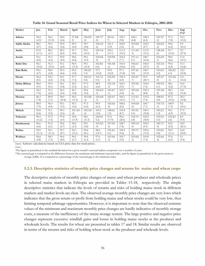
56

Table 14: Grand Seasonal Retail Price Indices for Wheat in Selected Markets in Ethiopia, 2002-2016


Adama 94.4 (6.5)1

96.6 (11.9)

94.0 (4.6)

97.4(8.5)

100.0(9.0)

100.7(7.0)

98.1(6.7)

105.1 (9.8)

106.1 (6.8)

108.3 (6.2)

101.9(7.2)

97.3 (7.8)

14.3 (15.2)


93.5 (4.6)

95.9 (3.6)

99.3 (4.4)

99.7 (4.8)

102.3(5.6)

101.3 (3.9)

102.9 (3.4)

103.0(4.5)

102.3 (4.7)

102.6(5.2)

99.0 (6.2)

9.4 (10.1)

Ambo 87.8 (11.1)

88.3 (6.7)

89.5 (8.2)

91.7 (9.0)

99.1 (10.5)

102.1(6.9)

105.1 (11.7)

111.5 (10.3)

111.4(9.5)

113.5 (12.1)

108.2(8.0)

91.7 (15.0)

23.7 (27.0)

Assela 93.1 (8.5)

91.3 (4.3)

93.9 (4.9)

94.6 (8.4)

99.1 (9.3)

102.0(6.9)

102.9(8.9)

105.4 (7.7)

107.1(10.7)

108.7 (10.4)

103.6(9.1)

98.4 (8.6)

17.4 (19.1)

Bahir Dar 96.1 (10.2)

91.3 (15.5)

93.1 (6.0)

96.0 (11.0)

99.1 (10.3)

102.8(10.6)

106.3(8.4)

101.0 (10.6)

106.6(10.9)

106.0 (10.7)

102.1(6.9)

99.6 (6.9)

15.3 (16.8)


98.0 (6.8)

95.3 (4.6)

95.2 (5.8)

100.2(13.3)

97.1 (10.2)

93.9 (12.2)

97.3 (13.8)

107.4(13.0)

106.7 (12.3)

103.0(15.2)

106.2(16.3)

12.2 (12.8)

Dessie 96.4 (8.1)

92.2 (6.0)

94.1 (5.4)

97.7 (7.2)

100.1(10.0)

103.7(10.5)

102.5(9.0)

105.3 (6.9)

105.2(7.7)

95.9 (20.7)

105.3(7.0)

101.5(6.5)

13.1 (14.2)

Debre Birhan 98.0 (9.1)

93.9 (8.1)

94.1 (3.8)

94.3 (5.2)

97.5 (6.1)

98.9 (6.0)

102.1(8.3)

105.1 (9.3)

103.9(6.7)

104.0 (7.6)

109.9(26.1)

98.1 (5.2)

16.0 (17.0)

Gonder 94.3 (7.0)

91.3 (6.2)

96.5 (5.6)

96.7 (5.8)

99.4 (5.2)

100.6(9.3)

105.4(7.1)

103.7 (5.0)

105.0(4.6)

105.2 (8.8)

103.3(8.9)

98.3 (5.8)

14.1 (15.4)

Hosana 86.3 (7.8)

89.8 (7.1)

94.0 (10.4)

94.5 (11.2)

103.2(8.4)

102.6(8.3)

102.5(7.7)

106.1 (10.1)

115.5(17.7)

110.2 (7.4)

108.0(12.0)

87.2 (10.2)

29.2 (33.8)

Jimma 98.9 (7.9)

96.3 (8.4)

95.1 (5.5)

95.3 (5.6)

97.3 (6.4)

99.9 (6.3)

102.6(6.8)

100.6 (8.2)

104.6(8.0)

104.7 (7.1)

103.7(5.3)

100.9 (7.3)

9.6 (10.1)

Mekele 93.8 (6.6)

91.1 (9.2)

99.3 (5.6)

101.3(4.8)

102.1(8.0)

103.3 (3.6)

108.6(11.5)

103.8 (8.7)

101.9(10.3)

100.3 (10.8)

100.2(11.2)

94.1 (6.9)

17.5 (19.2)

Nekemte 99.4 (11.2)

97.2 (7.6)

97.8 (4.5)

95.8 (11.9)

98.1 (11.5)

100.9(15.2)

97.6 (17.9)

99.6 (20.6)

104.7(16.8)

102.2 (18.0)

103.9(14.3)

102.4(12.6)

8.9 (9.3)


91.2 (6.1)

92.6 (6.7)

94.6 (5.3)

99.1 (5.8)

103.9(5.9)

107.0(5.5)

108.7 (7.8)

109.1(4.9)

109.5 (9.3)

100.7(7.9)

92.9 (6.9)

18.9 (20.1)

Woliso 92.9 (11.3)

95.1 (11.3)

95.7 (8.7)

92.3 (15.1)

95.4 (8.1)

98.0 (12.7)

105.4(10.1)

109.2 (9.6)

109.7(7.2)

109.4 (13.9)

103.8(10.8)

92.9 (11.1)

16.8 (18.0)

Woldeya 96.8 (4.8)

98.3 (7.4)

96.6 (8.6)

96.9 (6.7)

99.4 (6.3)

97.6 (5.1)

101.0(6.3)

105.7 (5.2)

103.6(6.2)

103.8 (7.2)

102.6(6.4)

97.6 (6.5)

9.1 (9.4)

Source: Authors’ calculations based on CSA price data for retail prices. Notes: 1The figure in parenthesis is the standard deviation for a given month’s seasonal indices computed over a number of years. 2 The seasonal gap is computed as the difference between the maximum and minimum seasonal index, and the figure in parenthesis is the gross return to

storage (GRS). It is computed as a percentage of the seasonal gap to the minimum index.

5.2.3. Descriptive statistics of monthly price changes and returns for maize and wheat crops

The descriptive analysis of monthly price changes of maize and wheat producer and wholesale prices

in selected maize markets in Ethiopia are provided in Tables 15-18, respectively. The simple

descriptive statistics that indicate the levels of returns and risks of holding maize stock in different

markets and market levels are clear. The observed average monthly price changes are very lows which

indicates that the gross return or profit from holding maize and wheat stocks could be very low, thus

limiting temporal arbitrage opportunities. However, it is important to note that the observed extreme

values of the minimum and maximum monthly price changes are hardly indicative of monthly storage

costs, a measure of the inefficiency of the maize storage system. The large positive and negative price

changes represent excessive windfall gains and losses in holding maize stocks at the producer and

wholesale levels. The results for wheat are presented in tables 17 and 18. Similar results are observed

in terms of the returns and risks of holding wheat stock at the producer and wholesale levels.

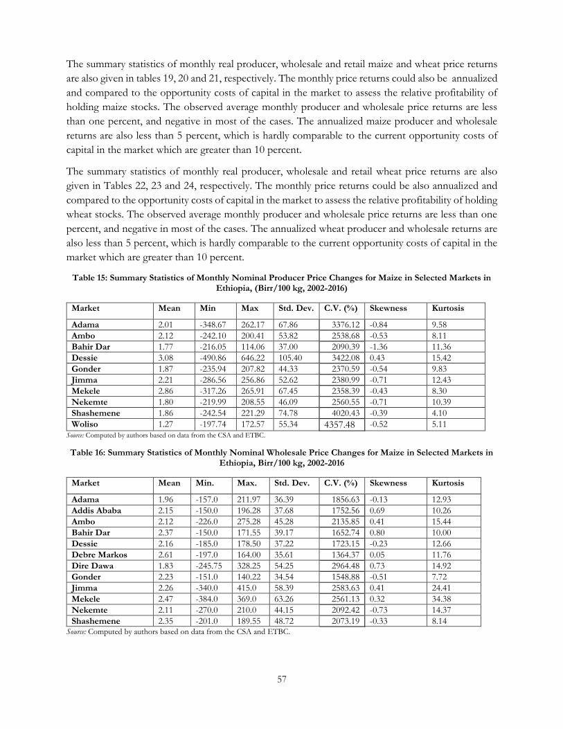
57

The summary statistics of monthly real producer, wholesale and retail maize and wheat price returns

are also given in tables 19, 20 and 21, respectively. The monthly price returns could also be annualized

and compared to the opportunity costs of capital in the market to assess the relative profitability of

holding maize stocks. The observed average monthly producer and wholesale price returns are less

than one percent, and negative in most of the cases. The annualized maize producer and wholesale

returns are also less than 5 percent, which is hardly comparable to the current opportunity costs of

capital in the market which are greater than 10 percent.

The summary statistics of monthly real producer, wholesale and retail wheat price returns are also

given in Tables 22, 23 and 24, respectively. The monthly price returns could be also annualized and

compared to the opportunity costs of capital in the market to assess the relative profitability of holding

wheat stocks. The observed average monthly producer and wholesale price returns are less than one

percent, and negative in most of the cases. The annualized wheat producer and wholesale returns are

also less than 5 percent, which is hardly comparable to the current opportunity costs of capital in the

market which are greater than 10 percent.

Table 15: Summary Statistics of Monthly Nominal Producer Price Changes for Maize in Selected Markets in Ethiopia, (Birr/100 kg, 2002-2016)

Market Mean Min Max Std. Dev. C.V. (%) Skewness Kurtosis

Adama 2.01 -348.67 262.17 67.86 3376.12 -0.84 9.58

Ambo 2.12 -242.10 200.41 53.82 2538.68 -0.53 8.11

Bahir Dar 1.77 -216.05 114.06 37.00 2090.39 -1.36 11.36

Dessie 3.08 -490.86 646.22 105.40 3422.08 0.43 15.42

Gonder 1.87 -235.94 207.82 44.33 2370.59 -0.54 9.83

Jimma 2.21 -286.56 256.86 52.62 2380.99 -0.71 12.43

Mekele 2.86 -317.26 265.91 67.45 2358.39 -0.43 8.30

Nekemte 1.80 -219.99 208.55 46.09 2560.55 -0.71 10.39

Shashemene 1.86 -242.54 221.29 74.78 4020.43 -0.39 4.10

Woliso 1.27 -197.74 172.57 55.34 4357.48 -0.52 5.11 Source: Computed by authors based on data from the CSA and ETBC.

Table 16: Summary Statistics of Monthly Nominal Wholesale Price Changes for Maize in Selected Markets in Ethiopia, Birr/100 kg, 2002-2016


Adama 1.96 -157.0 211.97 36.39 1856.63 -0.13 12.93

Addis Ababa 2.15 -150.0 196.28 37.68 1752.56 0.69 10.26

Ambo 2.12 -226.0 275.28 45.28 2135.85 0.41 15.44

Bahir Dar 2.37 -150.0 171.55 39.17 1652.74 0.80 10.00

Dessie 2.16 -185.0 178.50 37.22 1723.15 -0.23 12.66

Debre Markos 2.61 -197.0 164.00 35.61 1364.37 0.05 11.76

Dire Dawa 1.83 -245.75 328.25 54.25 2964.48 0.73 14.92

Gonder 2.23 -151.0 140.22 34.54 1548.88 -0.51 7.72

Jimma 2.26 -340.0 415.0 58.39 2583.63 0.41 24.41

Mekele 2.47 -384.0 369.0 63.26 2561.13 0.32 34.38

Nekemte 2.11 -270.0 210.0 44.15 2092.42 -0.73 14.37

Shashemene 2.35 -201.0 189.55 48.72 2073.19 -0.33 8.14 Source: Computed by authors based on data from the CSA and ETBC.

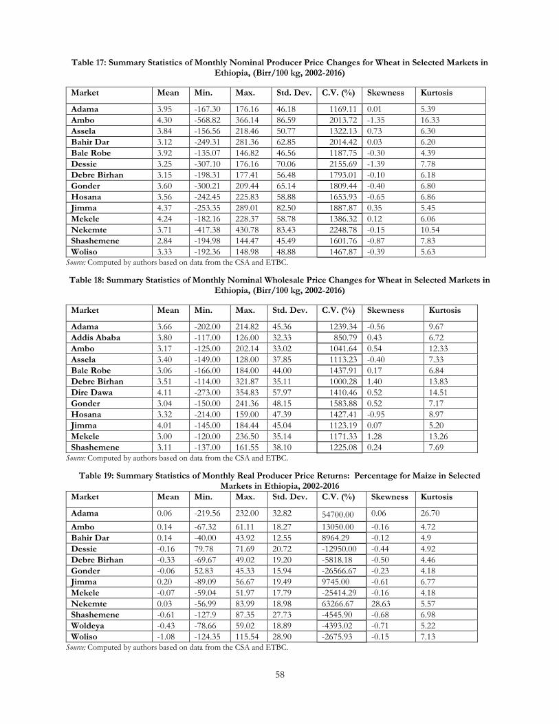
58

Table 17: Summary Statistics of Monthly Nominal Producer Price Changes for Wheat in Selected Markets in Ethiopia, (Birr/100 kg, 2002-2016)


Adama 3.95 -167.30 176.16 46.18 1169.11 0.01 5.39

Ambo 4.30 -568.82 366.14 86.59 2013.72 -1.35 16.33

Assela 3.84 -156.56 218.46 50.77 1322.13 0.73 6.30

Bahir Dar 3.12 -249.31 281.36 62.85 2014.42 0.03 6.20

Bale Robe 3.92 -135.07 146.82 46.56 1187.75 -0.30 4.39

Dessie 3.25 -307.10 176.16 70.06 2155.69 -1.39 7.78

Debre Birhan 3.15 -198.31 177.41 56.48 1793.01 -0.10 6.18

Gonder 3.60 -300.21 209.44 65.14 1809.44 -0.40 6.80

Hosana 3.56 -242.45 225.83 58.88 1653.93 -0.65 6.86

Jimma 4.37 -253.35 289.01 82.50 1887.87 0.35 5.45

Mekele 4.24 -182.16 228.37 58.78 1386.32 0.12 6.06

Nekemte 3.71 -417.38 430.78 83.43 2248.78 -0.15 10.54

Shashemene 2.84 -194.98 144.47 45.49 1601.76 -0.87 7.83

Woliso 3.33 -192.36 148.98 48.88 1467.87 -0.39 5.63 Source: Computed by authors based on data from the CSA and ETBC.

Table 18: Summary Statistics of Monthly Nominal Wholesale Price Changes for Wheat in Selected Markets in Ethiopia, (Birr/100 kg, 2002-2016)


Adama 3.66 -202.00 214.82 45.36 1239.34 -0.56 9.67

Addis Ababa 3.80 -117.00 126.00 32.33 850.79 0.43 6.72

Ambo 3.17 -125.00 202.14 33.02 1041.64 0.54 12.33

Assela 3.40 -149.00 128.00 37.85 1113.23 -0.40 7.33

Bale Robe 3.06 -166.00 184.00 44.00 1437.91 0.17 6.84

Debre Birhan 3.51 -114.00 321.87 35.11 1000.28 1.40 13.83

Dire Dawa 4.11 -273.00 354.83 57.97 1410.46 0.52 14.51

Gonder 3.04 -150.00 241.36 48.15 1583.88 0.52 7.17

Hosana 3.32 -214.00 159.00 47.39 1427.41 -0.95 8.97

Jimma 4.01 -145.00 184.44 45.04 1123.19 0.07 5.20

Mekele 3.00 -120.00 236.50 35.14 1171.33 1.28 13.26

Shashemene 3.11 -137.00 161.55 38.10 1225.08 0.24 7.69 Source: Computed by authors based on data from the CSA and ETBC.

Table 19: Summary Statistics of Monthly Real Producer Price Returns: Percentage for Maize in Selected Markets in Ethiopia, 2002-2016


Adama 0.06 -219.56 232.00 32.82 54700.00 0.06 26.70

Ambo 0.14 -67.32 61.11 18.27 13050.00 -0.16 4.72

Bahir Dar 0.14 -40.00 43.92 12.55 8964.29 -0.12 4.9

Dessie -0.16 79.78 71.69 20.72 -12950.00 -0.44 4.92

Debre Birhan -0.33 -69.67 49.02 19.20 -5818.18 -0.50 4.46

Gonder -0.06 52.83 45.33 15.94 -26566.67 -0.23 4.18

Jimma 0.20 -89.09 56.67 19.49 9745.00 -0.61 6.77

Mekele -0.07 -59.04 51.97 17.79 -25414.29 -0.16 4.18

Nekemte 0.03 -56.99 83.99 18.98 63266.67 28.63 5.57

Shashemene -0.61 -127.9 87.35 27.73 -4545.90 -0.68 6.98

Woldeya -0.43 -78.66 59.02 18.89 -4393.02 -0.71 5.22

Woliso -1.08 -124.35 115.54 28.90 -2675.93 -0.15 7.13 Source: Computed by authors based on data from the CSA and ETBC.

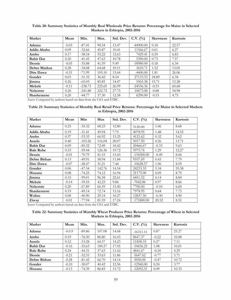
59

Table 20: Summary Statistics of Monthly Real Wholesale Price Returns: Percentage for Maize in Selected Markets in Ethiopia, 2002-2016


Adama -0.03 -87.41 90.54 13.47 -44900.00 0.18 22.57

Addis Ababa 0.09 -32.66 45.87 10.41 11566.67 0.61 6.27

Ambo 0.17 -38.54 55.22 12.63 7429.41 0.59 6.83

Bahir Dar 0.20 -41.45 47.63 10.78 5390.00 0.73 7.57

Dessie -0.05 -35.88 41.59 9.49 -18980.00 0.18 6.34

Debre Markos 0.28 -34.08 64.68 10.11 3610.71 1.52 13.05

Dire Dawa -0.31 -71.99 105.10 13.64 -4400.00 1.81 26.06

Gonder 0.03 -31.35 36.42 8.14 27133.33 24.89 6.34

Jimma 0.26 -65.03 85.85 14.47 5565.38 15.71 12.28

Mekele -0.11 -238.73 225.65 26.99 -24536.36 -0.53 60.68

Nekemte 0.26 -241.88 222.72 27.75 10673.08 -0.88 54.98

Shashemene 0.20 -44.77 37.30 12.58 6290.00 -0.53 4.75 Source: Computed by authors based on data from the CSA and ETBC.

Table 21: Summary Statistics of Monthly Real Retail Price Returns: Percentage for Maize in Selected Markets in Ethiopia, 2002-2016

Market Mean Min Max Std. Dev. C.V. (%) Skewness Kurtosis

Adama 0.25 -35.32 68.23 12.80 5120.00 1.06 8.68

Addis Ababa 0.19 -31.41 49.94 7.75 4078.95 1.48 14.52

Ambo 0.37 -53.33 66.92 15.25 4121.62 0.32 5.62

Assela 0.40 -103.26 116.04 20.07 5017.50 0.26 13.71

Bahir Dar 0.09 -85.32 72.49 18.42 20466.67 -0.33 9.63

Bale Robe 0.33 -59.44 126.36 19.72 5975.76 1.29 12.27

Dessie -0.01 -70.79 41.53 13.43 -134300.00 -0.49 8.06

Debre Birhan 0.13 -49.91 58.94 11.84 9107.69 0.43 7.79

Dire Dawa -0.07 -28.47 31.21 7.44 -10628.57 1.06 8.59

Gonder 0.06 -47.54 142.76 14.54 24233.33 5.34 55.38

Hosana 0.08 -74.25 74.12 16.94 21175.00 0.09 8.79

Jimma 0.33 -99.01 96.58 22.61 6851.52 0.14 8.84

Mekele -0.14 -39.55 42.23 9.86 -7042.86 0.97 8.66

Nekemte 0.20 -67.89 66.59 15.40 7700.00 -0.10 6.60

Shashemene 0.19 -49.14 72.74 15.16 7978.95 0.64 7.73

Woliso 0.08 -40.90 29.14 10.27 12837.50 -0.30 4.90

Ziway -0.01 -77.94 81.59 17.24 -172400.00 20.52 8.55 Source: Computed by authors based on data from the CSA and ETBC.

Table 22: Summary Statistics of Monthly Wheat Producer Price Returns: Percentage of Wheat in Selected Markets in Ethiopia, 2002-2016


Adama -0.0.9 -89.86 107.08 14.68 -16311.11 0.87 25.27

Ambo 0.19 -76.50 86.80 16.43 8647.37 -0.22 10.08

Assela 0.12 -53.28 64.57 14.23 11858.33 0.27 7.11

Bahir Dar -0.16 -55.63 100.57 17.05 -10656.25 1.08 10.01

Bale Robe 0.24 -44.31 37.63 11.62 4841.67 -0.24 4.29

Dessie -0.21 -52.55 33.63 11.86 -5647.62 -0.77 5.71

Debre Birhan -0.28 -81.42 66.70 14.14 -5050.00 -0.47 10.72

Gonder -0.10 -30.07 40.42 12.56 -12560.00 0.24 3.77

Hosana -0.13 -74.39 86.83 15.72 -12092.31 0.09 10.33

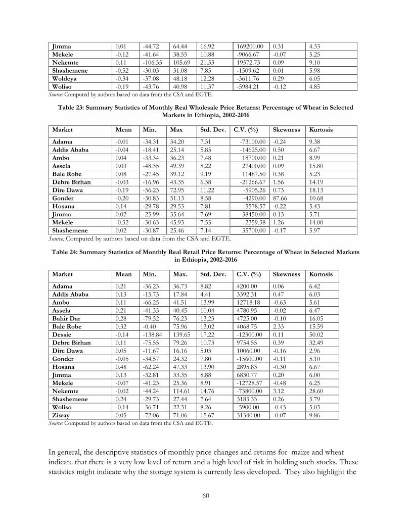
60

Jimma 0.01 -44.72 64.44 16.92 169200.00 0.31 4.33

Mekele -0.12 -41.64 38.55 10.88 -9066.67 -0.07 5.25

Nekemte 0.11 -106.35 105.69 21.53 19572.73 0.09 9.10

Shashemene -0.52 -30.03 31.08 7.85 -1509.62 0.01 5.98

Woldeya -0.34 -37.08 48.18 12.28 -3611.76 0.29 6.05

Woliso -0.19 -43.76 40.98 11.37 -5984.21 -0.12 4.85 Source: Computed by authors based on data from the CSA and EGTE.

Table 23: Summary Statistics of Monthly Real Wholesale Price Returns: Percentage of Wheat in Selected Markets in Ethiopia, 2002-2016

Market Mean Min. Max Std. Dev. C.V. (%) Skewness Kurtosis

Adama -0.01 -34.31 34.20 7.31 -73100.00 -0.24 9.38

Addis Ababa -0.04 -18.41 25.14 5.85 -14625.00 0.50 6.67

Ambo 0.04 -33.34 36.23 7.48 18700.00 0.21 8.99

Assela 0.03 -48.35 49.39 8.22 27400.00 0.09 15.80

Bale Robe 0.08 -27.45 39.12 9.19 11487.50 0.38 5.23

Debre Birhan -0.03 -16.96 43.35 6.38 -21266.67 1.56 14.19

Dire Dawa -0.19 -56.23 72.95 11.22 -5905.26 0.73 18.13

Gonder -0.20 -30.83 51.13 8.58 -4290.00 87.66 10.68

Hosana 0.14 -29.78 29.53 7.81 5578.57 -0.22 5.43

Jimma 0.02 -25.99 35.64 7.69 38450.00 0.13 5.71

Mekele -0.32 -30.63 45.93 7.55 -2359.38 1.26 14.00

Shashemene 0.02 -30.87 25.46 7.14 35700.00 -0.17 5.97

Source: Computed by authors based on data from the CSA and EGTE.

Table 24: Summary Statistics of Monthly Real Retail Price Returns: Percentage of Wheat in Selected Markets in Ethiopia, 2002-2016


Adama 0.21 -36.23 36.73 8.82 4200.00 0.06 6.42

Addis Ababa 0.13 -15.73 17.84 4.41 3392.31 0.47 6.03

Ambo 0.11 -66.25 41.51 13.99 12718.18 -0.63 5.61

Assela 0.21 -41.33 40.45 10.04 4780.95 -0.02 6.47

Bahir Dar 0.28 -79.52 76.23 13.23 4725.00 -0.10 16.05

Bale Robe 0.32 -0.40 75.96 13.02 4068.75 2.33 15.59

Dessie -0.14 -138.84 139.65 17.22 -12300.00 0.11 50.02

Debre Birhan 0.11 -75.55 79.26 10.73 9754.55 0.39 32.49

Dire Dawa 0.05 -11.67 16.16 5.03 10060.00 -0.16 2.96

Gonder -0.05 -34.57 24.32 7.80 -15600.00 -0.11 5.10

Hosana 0.48 -62.24 47.33 13.90 2895.83 -0.30 6.67

Jimma 0.13 -32.81 33.35 8.88 6830.77 0.20 6.00

Mekele -0.07 -41.23 25.36 8.91 -12728.57 -0.48 6.25

Nekemte -0.02 -44.24 114.61 14.76 -73800.00 3.12 28.60

Shashemene 0.24 -29.73 27.44 7.64 3183.33 0.26 5.79

Woliso -0.14 -36.71 22.31 8.26 -5900.00 -0.45 5.03

Ziway 0.05 -72.06 71.06 15.67 31340.00 -0.07 9.86 Source: Computed by authors based on data from the CSA and EGTE.

In general, the descriptive statistics of monthly price changes and returns for maize and wheat

indicate that there is a very low level of return and a high level of risk in holding such stocks. These

statistics might indicate why the storage system is currently less developed. They also highlight the

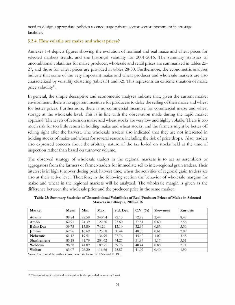
61

need to design appropriate policies to encourage private sector sector investment in strorage

facilities.

5.2.4. How volatile are maize and wheat prices?

Annexes 1-4 depicts figures showing the evolution of nominal and real maize and wheat prices for

selected markets trends, and the historical volatility for 2001-2016. The summary statistics of

unconditional volatilities for maize producer, wholesale and retail prices are summarized in tables 25-

27, and those for wheat prices are provided in tables 28-30. Furthermore, the econometric analyses

indicate that some of the very important maize and wheat producer and wholesale markets are also

characterized by volatility clustering (tables 31 and 32). This represents an extreme situation of maize

price volatility14.

In general, the simple descriptive and econometric analyses indicate that, given the current market

environment, there is no apparent incentive for producers to delay the selling of their maize and wheat

for better prices. Furthermore, there is no commercial incentive for commercial maize and wheat

storage at the wholesale level. This is in line with the observation made during the rapid market

appraisal. The levels of return on maize and wheat stocks are very low and highly volatile. There is too

much risk for too little return in holding maize and wheat stocks, and the farmers might be better off

selling right after the harvest. The wholesale traders also indicated that they are not interested in

holding stocks of maize and wheat for several reasons, including the risk of price drops. Also, traders

also expressed concern about the arbitrary nature of the tax levied on stocks held at the time of

inspection rather than based on turnover volume.

The observed strategy of wholesale traders in the regional markets is to act as assemblers or

aggregators from the farmers or farmer-traders for immediate sell to inter-regional grain traders. Their

interest is in high turnover during peak harvest time, when the activities of regional grain traders are

also at their active level. Therefore, in the following section the behavior of wholesale margins for

maize and wheat in the regional markets will be analyzed. The wholesale margin is given as the

difference between the wholesale price and the producer price in the same market.

Table 25: Summary Statistics of Unconditional Volatilities of Real Producer Prices of Maize in Selected Markets in Ethiopia, 2002-2016


Adama 98.84 28.58 340.94 72.13 72.98 2.44 8.47

Ambo 62.91 24.39 122.50 23.60 37.51 0.60 2.56

Bahir Dar 39.75 15.80 74.29 13.10 32.96 0.83 3.36

Jimma 62.96 16.69 125.58 30.44 48.35 0.61 2.09

Nekemte 61.12 19.51 136.99 27.76 45.42 1.07 3.45

Shashemene 85.18 31.79 204.62 44.27 51.97 1.17 3.51

Woldeya 98.38 41.89 189.75 39.78 40.44 0.88 2.71


14 The evolution of maize and wheat prices is also provided in annexes 1 to 4.

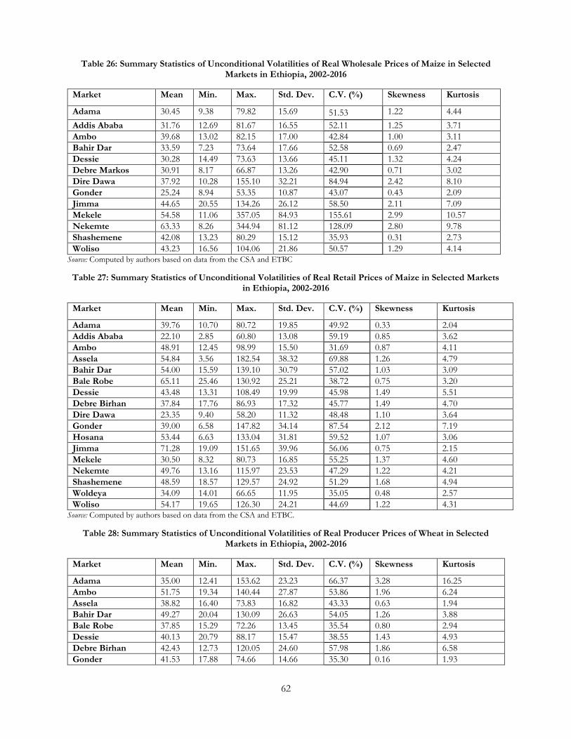
62

Table 26: Summary Statistics of Unconditional Volatilities of Real Wholesale Prices of Maize in Selected Markets in Ethiopia, 2002-2016


Adama 30.45 9.38 79.82 15.69 51.53 1.22 4.44

Addis Ababa 31.76 12.69 81.67 16.55 52.11 1.25 3.71

Ambo 39.68 13.02 82.15 17.00 42.84 1.00 3.11

Bahir Dar 33.59 7.23 73.64 17.66 52.58 0.69 2.47

Dessie 30.28 14.49 73.63 13.66 45.11 1.32 4.24

Debre Markos 30.91 8.17 66.87 13.26 42.90 0.71 3.02

Dire Dawa 37.92 10.28 155.10 32.21 84.94 2.42 8.10

Gonder 25.24 8.94 53.35 10.87 43.07 0.43 2.09

Jimma 44.65 20.55 134.26 26.12 58.50 2.11 7.09

Mekele 54.58 11.06 357.05 84.93 155.61 2.99 10.57

Nekemte 63.33 8.26 344.94 81.12 128.09 2.80 9.78

Shashemene 42.08 13.23 80.29 15.12 35.93 0.31 2.73

Woliso 43.23 16.56 104.06 21.86 50.57 1.29 4.14 Source: Computed by authors based on data from the CSA and ETBC

Table 27: Summary Statistics of Unconditional Volatilities of Real Retail Prices of Maize in Selected Markets in Ethiopia, 2002-2016


Adama 39.76 10.70 80.72 19.85 49.92 0.33 2.04

Addis Ababa 22.10 2.85 60.80 13.08 59.19 0.85 3.62

Ambo 48.91 12.45 98.99 15.50 31.69 0.87 4.11

Assela 54.84 3.56 182.54 38.32 69.88 1.26 4.79

Bahir Dar 54.00 15.59 139.10 30.79 57.02 1.03 3.09

Bale Robe 65.11 25.46 130.92 25.21 38.72 0.75 3.20

Dessie 43.48 13.31 108.49 19.99 45.98 1.49 5.51

Debre Birhan 37.84 17.76 86.93 17.32 45.77 1.49 4.70

Dire Dawa 23.35 9.40 58.20 11.32 48.48 1.10 3.64

Gonder 39.00 6.58 147.82 34.14 87.54 2.12 7.19

Hosana 53.44 6.63 133.04 31.81 59.52 1.07 3.06

Jimma 71.28 19.09 151.65 39.96 56.06 0.75 2.15

Mekele 30.50 8.32 80.73 16.85 55.25 1.37 4.60

Nekemte 49.76 13.16 115.97 23.53 47.29 1.22 4.21

Shashemene 48.59 18.57 129.57 24.92 51.29 1.68 4.94

Woldeya 34.09 14.01 66.65 11.95 35.05 0.48 2.57


Table 28: Summary Statistics of Unconditional Volatilities of Real Producer Prices of Wheat in Selected Markets in Ethiopia, 2002-2016


Adama 35.00 12.41 153.62 23.23 66.37 3.28 16.25

Ambo 51.75 19.34 140.44 27.87 53.86 1.96 6.24

Assela 38.82 16.40 73.83 16.82 43.33 0.63 1.94

Bahir Dar 49.27 20.04 130.09 26.63 54.05 1.26 3.88

Bale Robe 37.85 15.29 72.26 13.45 35.54 0.80 2.94

Dessie 40.13 20.79 88.17 15.47 38.55 1.43 4.93

Debre Birhan 42.43 12.73 120.05 24.60 57.98 1.86 6.58

Gonder 41.53 17.88 74.66 14.66 35.30 0.16 1.93

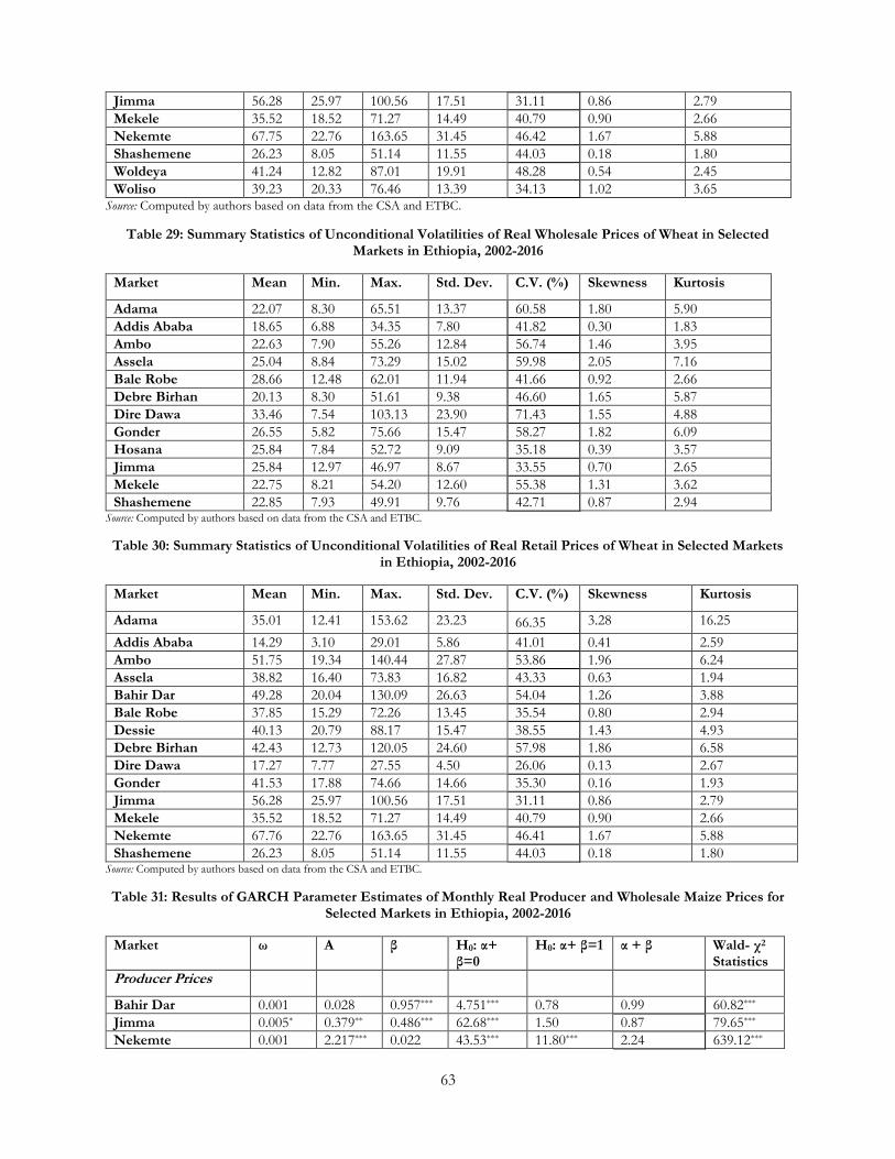
63

Jimma 56.28 25.97 100.56 17.51 31.11 0.86 2.79

Mekele 35.52 18.52 71.27 14.49 40.79 0.90 2.66

Nekemte 67.75 22.76 163.65 31.45 46.42 1.67 5.88

Shashemene 26.23 8.05 51.14 11.55 44.03 0.18 1.80

Woldeya 41.24 12.82 87.01 19.91 48.28 0.54 2.45


Table 29: Summary Statistics of Unconditional Volatilities of Real Wholesale Prices of Wheat in Selected Markets in Ethiopia, 2002-2016


Adama 22.07 8.30 65.51 13.37 60.58 1.80 5.90

Addis Ababa 18.65 6.88 34.35 7.80 41.82 0.30 1.83

Ambo 22.63 7.90 55.26 12.84 56.74 1.46 3.95

Assela 25.04 8.84 73.29 15.02 59.98 2.05 7.16

Bale Robe 28.66 12.48 62.01 11.94 41.66 0.92 2.66

Debre Birhan 20.13 8.30 51.61 9.38 46.60 1.65 5.87

Dire Dawa 33.46 7.54 103.13 23.90 71.43 1.55 4.88

Gonder 26.55 5.82 75.66 15.47 58.27 1.82 6.09

Hosana 25.84 7.84 52.72 9.09 35.18 0.39 3.57

Jimma 25.84 12.97 46.97 8.67 33.55 0.70 2.65

Mekele 22.75 8.21 54.20 12.60 55.38 1.31 3.62


Table 30: Summary Statistics of Unconditional Volatilities of Real Retail Prices of Wheat in Selected Markets in Ethiopia, 2002-2016


Adama 35.01 12.41 153.62 23.23 66.35 3.28 16.25

Addis Ababa 14.29 3.10 29.01 5.86 41.01 0.41 2.59

Ambo 51.75 19.34 140.44 27.87 53.86 1.96 6.24

Assela 38.82 16.40 73.83 16.82 43.33 0.63 1.94

Bahir Dar 49.28 20.04 130.09 26.63 54.04 1.26 3.88

Bale Robe 37.85 15.29 72.26 13.45 35.54 0.80 2.94

Dessie 40.13 20.79 88.17 15.47 38.55 1.43 4.93

Debre Birhan 42.43 12.73 120.05 24.60 57.98 1.86 6.58

Dire Dawa 17.27 7.77 27.55 4.50 26.06 0.13 2.67

Gonder 41.53 17.88 74.66 14.66 35.30 0.16 1.93

Jimma 56.28 25.97 100.56 17.51 31.11 0.86 2.79

Mekele 35.52 18.52 71.27 14.49 40.79 0.90 2.66

Nekemte 67.76 22.76 163.65 31.45 46.41 1.67 5.88


Table 31: Results of GARCH Parameter Estimates of Monthly Real Producer and Wholesale Maize Prices for Selected Markets in Ethiopia, 2002-2016

Market ω Α β H0: α+ β=0

H0: α+ β=1 α + β Wald- χ2 Statistics

Producer Prices

Bahir Dar 0.001 0.028 0.957*** 4.751*** 0.78 0.99 60.82***

Jimma 0.005* 0.379** 0.486*** 62.68*** 1.50 0.87 79.65***

Nekemte 0.001 2.217*** 0.022 43.53*** 11.80*** 2.24 639.12***

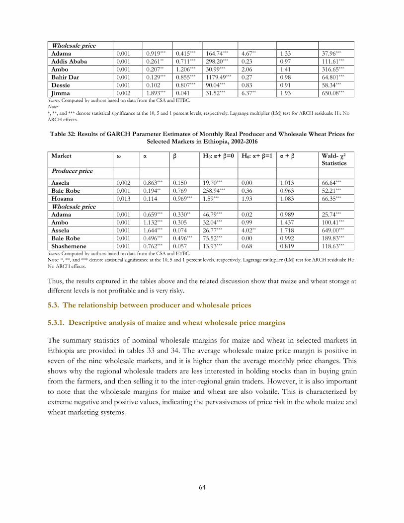
64

Wholesale price

Adama 0.001 0.919*** 0.415*** 164.74*** 4.67** 1.33 37.96***

Addis Ababa 0.001 0.261** 0.711*** 298.20*** 0.23 0.97 111.61***

Ambo 0.001 0.207** 1.206*** 30.99*** 2.06 1.41 316.65***

Bahir Dar 0.001 0.129*** 0.855*** 1179.49*** 0.27 0.98 64.801***

Dessie 0.001 0.102 0.807*** 90.04*** 0.83 0.91 58.34***

Jimma 0.002 1.893*** 0.041 31.52*** 6.37** 1.93 650.08*** Source: Computed by authors based on data from the CSA and ETBC.

Note:

*, **, and *** denote statistical significance at the 10, 5 and 1 percent levels, respectively. Lagrange multiplier (LM) test for ARCH residuals: H0: No

ARCH effects.

Table 32: Results of GARCH Parameter Estimates of Monthly Real Producer and Wholesale Wheat Prices for Selected Markets in Ethiopia, 2002-2016

Market ω α β H0: α+ β=0 H0: α+ β=1 α + β Wald- χ2 Statistics

Producer price

Assela 0.002 0.863*** 0.150 19.70*** 0.00 1.013 66.64***

Bale Robe 0.001 0.194** 0.769 258.94*** 0.36 0.963 52.21***

Hosana 0.013 0.114 0.969*** 1.59*** 1.93 1.083 66.35***

Wholesale price

Adama 0.001 0.659*** 0.330** 46.79*** 0.02 0.989 25.74***

Ambo 0.001 1.132*** 0.305 32.04*** 0.99 1.437 100.41***

Assela 0.001 1.644*** 0.074 26.77*** 4.02** 1.718 649.00***

Bale Robe 0.001 0.496*** 0.496*** 75.52*** 0.00 0.992 189.83***

Shashemene 0.001 0.762*** 0.057 13.93*** 0.68 0.819 118.63*** Source: Computed by authors based on data from the CSA and ETBC.

Note: *, **, and *** denote statistical significance at the 10, 5 and 1 percent levels, respectively. Lagrange multiplier (LM) test for ARCH residuals: H0:

No ARCH effects.

Thus, the results captured in the tables above and the related discussion show that maize and wheat storage at

different levels is not profitable and is very risky.

5.3. The relationship between producer and wholesale prices

5.3.1. Descriptive analysis of maize and wheat wholesale price margins

The summary statistics of nominal wholesale margins for maize and wheat in selected markets in

Ethiopia are provided in tables 33 and 34. The average wholesale maize price margin is positive in

seven of the nine wholesale markets, and it is higher than the average monthly price changes. This

shows why the regional wholesale traders are less interested in holding stocks than in buying grain

from the farmers, and then selling it to the inter-regional grain traders. However, it is also important

to note that the wholesale margins for maize and wheat are also volatile. This is characterized by

extreme negative and positive values, indicating the pervasiveness of price risk in the whole maize and

wheat marketing systems.

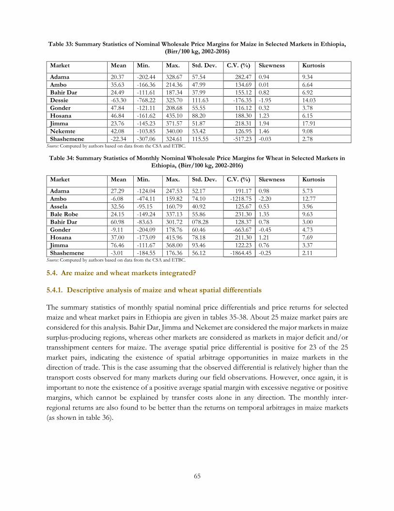
65

Table 33: Summary Statistics of Nominal Wholesale Price Margins for Maize in Selected Markets in Ethiopia, (Birr/100 kg, 2002-2016)


Adama 20.37 -202.44 328.67 57.54 282.47 0.94 9.34

Ambo 35.63 -166.36 214.36 47.99 134.69 0.01 6.64

Bahir Dar 24.49 -111.61 187.34 37.99 155.12 0.82 6.92

Dessie -63.30 -768.22 325.70 111.63 -176.35 -1.95 14.03

Gonder 47.84 -121.11 208.68 55.55 116.12 0.32 3.78

Hosana 46.84 -161.62 435.10 88.20 188.30 1.23 6.15

Jimma 23.76 -145.23 371.57 51.87 218.31 1.94 17.91

Nekemte 42.08 -103.85 340.00 53.42 126.95 1.46 9.08

Shashemene -22.34 -307.06 324.61 115.55 -517.23 -0.03 2.78 Source: Computed by authors based on data from the CSA and ETBC.

Table 34: Summary Statistics of Monthly Nominal Wholesale Price Margins for Wheat in Selected Markets in Ethiopia, (Birr/100 kg, 2002-2016)


Adama 27.29 -124.04 247.53 52.17 191.17 0.98 5.73

Ambo -6.08 -474.11 159.82 74.10 -1218.75 -2.20 12.77

Assela 32.56 -95.15 160.79 40.92 125.67 0.53 3.96

Bale Robe 24.15 -149.24 337.13 55.86 231.30 1.35 9.63

Bahir Dar 60.98 -83.63 301.72 078.28 128.37 0.78 3.00

Gonder -9.11 -204.09 178.76 60.46 -663.67 -0.45 4.73

Hosana 37.00 -173.09 415.96 78.18 211.30 1.21 7.69

Jimma 76.46 -111.67 368.00 93.46 122.23 0.76 3.37

Shashemene -3.01 -184.55 176.36 56.12 -1864.45 -0.25 2.11 Source: Computed by authors based on data from the CSA and ETBC.

5.4. Are maize and wheat markets integrated?

5.4.1. Descriptive analysis of maize and wheat spatial differentials

The summary statistics of monthly spatial nominal price differentials and price returns for selected

maize and wheat market pairs in Ethiopia are given in tables 35-38. About 25 maize market pairs are

considered for this analysis. Bahir Dar, Jimma and Nekemet are considered the major markets in maize

surplus-producing regions, whereas other markets are considered as markets in major deficit and/or

transshipment centers for maize. The average spatial price differential is positive for 23 of the 25

market pairs, indicating the existence of spatial arbitrage opportunities in maize markets in the

direction of trade. This is the case assuming that the observed differential is relatively higher than the

transport costs observed for many markets during our field observations. However, once again, it is

important to note the existence of a positive average spatial margin with excessive negative or positive

margins, which cannot be explained by transfer costs alone in any direction. The monthly inter-

regional returns are also found to be better than the returns on temporal arbitrages in maize markets

(as shown in table 36).

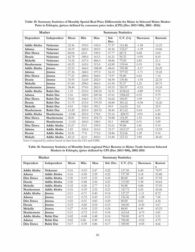
66

Table 35: Summary Statistics of Monthly Spatial Real Price Differentials for Maize in Selected Maize Market Pairs in Ethiopia, (prices deflated by consumer price index (CPI) (Dec 2011=100), 2002- 2016)

Market Summary Statistics

Dependent Independent Mean Min Max Std. Dev.

C.V. (%) Skewness Kurtosis

Addis Ababa Nekemet 32.36 -195.0 145.0 37.37 115.48 -1.38 11.23

Adama Nekemet 34.19 -202.0 202.0 45.36 132.67 -1.39 10.06

Dire Dawa Nekemet 84.04 -65.0 330.0 57.77 68.74 0.68 5.02

Dessie Nekemet 42.78 -180.0 163.5 41.21 96.33 -0.95 8.10

Mekelle Nekemet 74.32 -107.0 486.0 58.86 79.20 2.85 21.1

Shashemene Nekemet 45.23 -165.0 315.0 62.89 139.04 0.33 5.56

Addis Ababa Jimma 25.53 -366.0 188.00 48.63 190.48 -2.17 26.29

Adama Jimma 27.36 -368.0 197.0 54.15 197.92 -1.71 19.22

Dire Dawa Jimma 77.21 -288.0 368.0 73.97 95.80 0.43 7.14

Dessie Jimma 35.95 -32.60 202.0 46.90 130.46 -1.95 22.35

Mekelle Jimma 67.60 -298.0 466.0 61.90 91.57 1.25 20.75

Shashemene Jimma 38.40 -370.0 282.0 69.53 181.07 -0.15 10.24

Addis Ababa Bahir Dar 1.33 -253.0 240.55 55.31 4158.65 -0.89 9.92

Adama Bahir Dar 3.16 -182.0 249.56 47.61 1506.65 0.35 9.79

Dire Dawa Bahir Dar 53.01 -146.0 311.55 56.62 106.81 1.09 7.27

Dessie Bahir Dar 11.75 -215.0 199.55 44.84 381.62 -0.38 10.26

Mekelle Bahir Dar 43.0 -158.0 392.1 49.9 116.05 3.0 25.9

Shashemene Bahir Dar 14.20 -203.0 269.55 58.45 411.62 0.54 6.91

Addis Ababa Shashemene -12.86 -253.0 178.0 55.16 -428.93 -0.91 6.40

Dire Dawa Shashemene 38.81 -101.0 294.75 59.88 154.29 1.55 8.01

Adama Shashemene -11.03 -160.0 148.0 45.1 -408.88 0.31 5.09

Dire Dawa Addis Ababa 51.67 -53.5 339.0 51.61 99.88 1.81 9.19

Adama Addis Ababa 1.83 -182.0 163.0 33.17 1812.57 -0.32 12.55

Dessie Addis Ababa 10.41 -77.0 173.0 32.86 315.66 1.29 9.16

Mekele Addis Ababa 42.12 -61.0 445.0 51.86 123.12 3.85 26.45 Source: Computed by authors based on data from the CSA and ETBC.

Table 36: Summary Statistics of Monthly Inter-regional Price Returns to Maize Trade between Selected Markets in Ethiopia, (price deflated by CPI (Dec 2011=100), 2002-2016


Dependent Independent Mean Min. Max. Std. Dev. C.V. (%) Skewness Kurtosis

Addis Ababa Nekemet 0.16 -0.53 2.47 0.22 137.50 6.40 70.97

Adama Addis Ababa 0.16 -0.50 2.39 0.22 137.50 5.18 55.88



Mekelle Addis Ababa 0.32 -0.26 2.77 0.31 96.88 4.88 37.05

Shashemene Addis Ababa 0.16 -0.39 2.32 0.23 143.75 4.25 42.46

Addis Ababa Jimma 0.11 -0.71 0.40 0.14 127.27 -1.11 8.72

Adama Jimma 0.11 -0.72 0.43 0.15 136.36 -1.28 7.56

Dire Dawa Jimma 0.25 -0.51 0.83 0.20 80.00 0.02 4.24

Dessie Jimma 0.15 -0.60 0.54 0.15 100.00 -0.30 5.67

Mekelle Jimma 0.27 -0.54 2.53 0.24 88.89 4.49 43.23

Shashemene Jimma 0.11 -0.72 0.53 0.18 163.64 -0.75 5.81

Addis Ababa Bahir Dar 0.02 -0.48 0.48 0.14 700.00 -0.71 5.51

Adama Bahir Dar 0.02 0.46 0.49 0.14 700.00 -0.52 4.79

Dire Dawa Bahir Dar 0.17 -0.39 0.86 0.17 100.00 -0.05 4.66

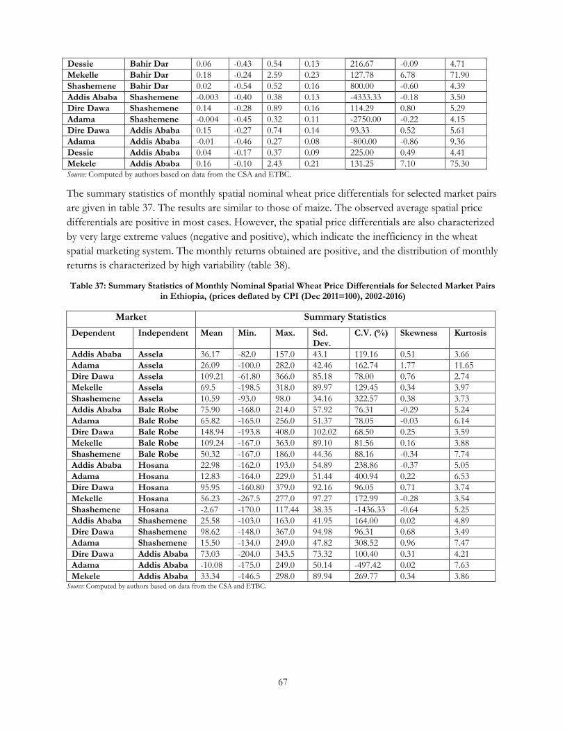
67

Dessie Bahir Dar 0.06 -0.43 0.54 0.13 216.67 -0.09 4.71

Mekelle Bahir Dar 0.18 -0.24 2.59 0.23 127.78 6.78 71.90

Shashemene Bahir Dar 0.02 -0.54 0.52 0.16 800.00 -0.60 4.39

Addis Ababa Shashemene -0.003 -0.40 0.38 0.13 -4333.33 -0.18 3.50


Adama Shashemene -0.004 -0.45 0.32 0.11 -2750.00 -0.22 4.15


Adama Addis Ababa -0.01 -0.46 0.27 0.08 -800.00 -0.86 9.36



The summary statistics of monthly spatial nominal wheat price differentials for selected market pairs

are given in table 37. The results are similar to those of maize. The observed average spatial price

differentials are positive in most cases. However, the spatial price differentials are also characterized

by very large extreme values (negative and positive), which indicate the inefficiency in the wheat

spatial marketing system. The monthly returns obtained are positive, and the distribution of monthly

returns is characterized by high variability (table 38).

Table 37: Summary Statistics of Monthly Nominal Spatial Wheat Price Differentials for Selected Market Pairs in Ethiopia, (prices deflated by CPI (Dec 2011=100), 2002-2016)


Dependent Independent Mean Min. Max. Std. Dev.

C.V. (%) Skewness Kurtosis

Addis Ababa Assela 36.17 -82.0 157.0 43.1 119.16 0.51 3.66

Adama Assela 26.09 -100.0 282.0 42.46 162.74 1.77 11.65

Dire Dawa Assela 109.21 -61.80 366.0 85.18 78.00 0.76 2.74

Mekelle Assela 69.5 -198.5 318.0 89.97 129.45 0.34 3.97

Shashemene Assela 10.59 -93.0 98.0 34.16 322.57 0.38 3.73

Addis Ababa Bale Robe 75.90 -168.0 214.0 57.92 76.31 -0.29 5.24

Adama Bale Robe 65.82 -165.0 256.0 51.37 78.05 -0.03 6.14

Dire Dawa Bale Robe 148.94 -193.8 408.0 102.02 68.50 0.25 3.59

Mekelle Bale Robe 109.24 -167.0 363.0 89.10 81.56 0.16 3.88

Shashemene Bale Robe 50.32 -167.0 186.0 44.36 88.16 -0.34 7.74

Addis Ababa Hosana 22.98 -162.0 193.0 54.89 238.86 -0.37 5.05

Adama Hosana 12.83 -164.0 229.0 51.44 400.94 0.22 6.53

Dire Dawa Hosana 95.95 -160.80 379.0 92.16 96.05 0.71 3.74

Mekelle Hosana 56.23 -267.5 277.0 97.27 172.99 -0.28 3.54

Shashemene Hosana -2.67 -170.0 117.44 38.35 -1436.33 -0.64 5.25

Addis Ababa Shashemene 25.58 -103.0 163.0 41.95 164.00 0.02 4.89


Adama Shashemene 15.50 -134.0 249.0 47.82 308.52 0.96 7.47


Adama Addis Ababa -10.08 -175.0 249.0 50.14 -497.42 0.02 7.63


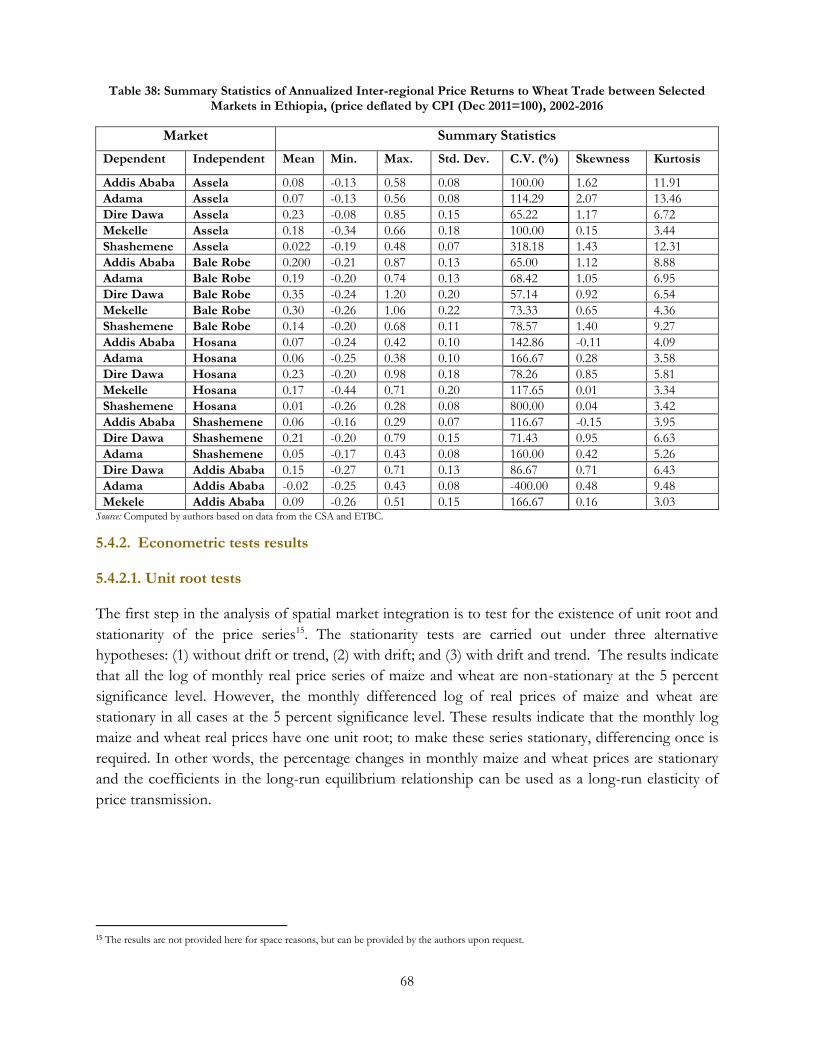
68

Table 38: Summary Statistics of Annualized Inter-regional Price Returns to Wheat Trade between Selected Markets in Ethiopia, (price deflated by CPI (Dec 2011=100), 2002-2016


Dependent Independent Mean Min. Max. Std. Dev. C.V. (%) Skewness Kurtosis

Addis Ababa Assela 0.08 -0.13 0.58 0.08 100.00 1.62 11.91

Adama Assela 0.07 -0.13 0.56 0.08 114.29 2.07 13.46

Dire Dawa Assela 0.23 -0.08 0.85 0.15 65.22 1.17 6.72

Mekelle Assela 0.18 -0.34 0.66 0.18 100.00 0.15 3.44

Shashemene Assela 0.022 -0.19 0.48 0.07 318.18 1.43 12.31

Addis Ababa Bale Robe 0.200 -0.21 0.87 0.13 65.00 1.12 8.88

Adama Bale Robe 0.19 -0.20 0.74 0.13 68.42 1.05 6.95

Dire Dawa Bale Robe 0.35 -0.24 1.20 0.20 57.14 0.92 6.54

Mekelle Bale Robe 0.30 -0.26 1.06 0.22 73.33 0.65 4.36

Shashemene Bale Robe 0.14 -0.20 0.68 0.11 78.57 1.40 9.27

Addis Ababa Hosana 0.07 -0.24 0.42 0.10 142.86 -0.11 4.09

Adama Hosana 0.06 -0.25 0.38 0.10 166.67 0.28 3.58

Dire Dawa Hosana 0.23 -0.20 0.98 0.18 78.26 0.85 5.81

Mekelle Hosana 0.17 -0.44 0.71 0.20 117.65 0.01 3.34

Shashemene Hosana 0.01 -0.26 0.28 0.08 800.00 0.04 3.42

Addis Ababa Shashemene 0.06 -0.16 0.29 0.07 116.67 -0.15 3.95


Adama Shashemene 0.05 -0.17 0.43 0.08 160.00 0.42 5.26


Adama Addis Ababa -0.02 -0.25 0.43 0.08 -400.00 0.48 9.48


5.4.2. Econometric tests results

5.4.2.1. Unit root tests

The first step in the analysis of spatial market integration is to test for the existence of unit root and

stationarity of the price series15. The stationarity tests are carried out under three alternative

hypotheses: (1) without drift or trend, (2) with drift; and (3) with drift and trend. The results indicate

that all the log of monthly real price series of maize and wheat are non-stationary at the 5 percent

significance level. However, the monthly differenced log of real prices of maize and wheat are

stationary in all cases at the 5 percent significance level. These results indicate that the monthly log

maize and wheat real prices have one unit root; to make these series stationary, differencing once is

required. In other words, the percentage changes in monthly maize and wheat prices are stationary

and the coefficients in the long-run equilibrium relationship can be used as a long-run elasticity of

price transmission.

15 The results are not provided here for space reasons, but can be provided by the authors upon request.

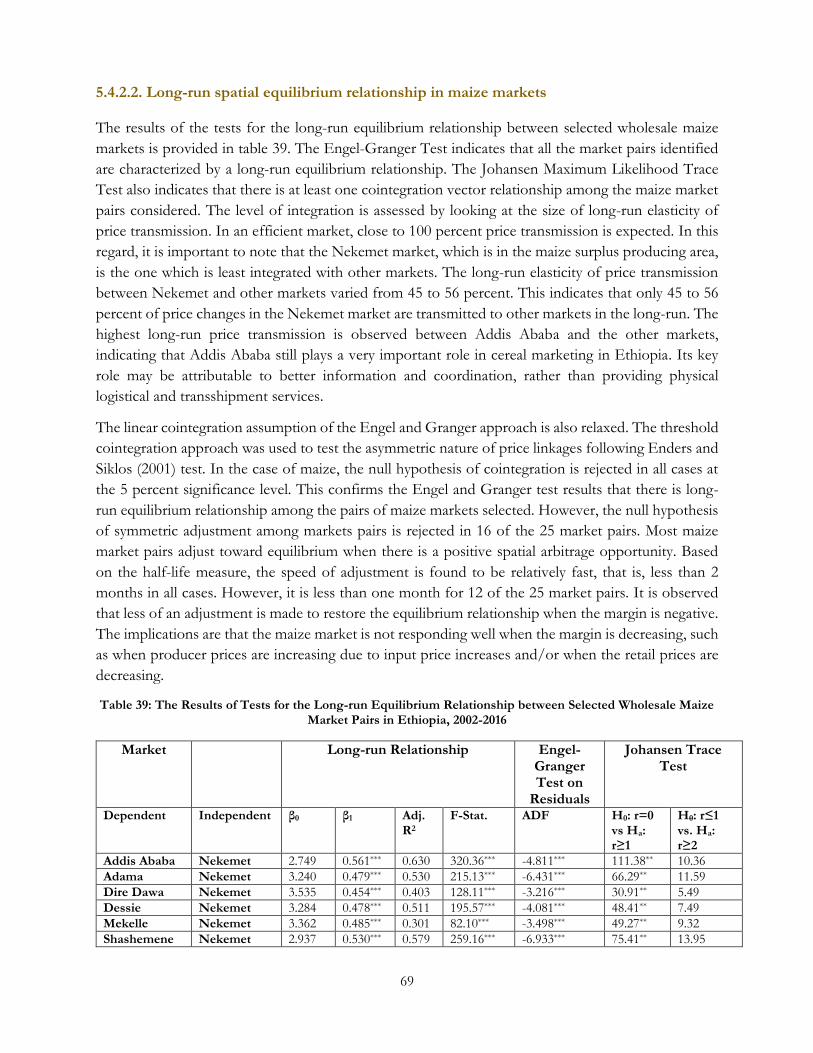
69

5.4.2.2. Long-run spatial equilibrium relationship in maize markets

The results of the tests for the long-run equilibrium relationship between selected wholesale maize

markets is provided in table 39. The Engel-Granger Test indicates that all the market pairs identified

are characterized by a long-run equilibrium relationship. The Johansen Maximum Likelihood Trace

Test also indicates that there is at least one cointegration vector relationship among the maize market

pairs considered. The level of integration is assessed by looking at the size of long-run elasticity of

price transmission. In an efficient market, close to 100 percent price transmission is expected. In this

regard, it is important to note that the Nekemet market, which is in the maize surplus producing area,

is the one which is least integrated with other markets. The long-run elasticity of price transmission

between Nekemet and other markets varied from 45 to 56 percent. This indicates that only 45 to 56

percent of price changes in the Nekemet market are transmitted to other markets in the long-run. The

highest long-run price transmission is observed between Addis Ababa and the other markets,

indicating that Addis Ababa still plays a very important role in cereal marketing in Ethiopia. Its key

role may be attributable to better information and coordination, rather than providing physical

logistical and transshipment services.

The linear cointegration assumption of the Engel and Granger approach is also relaxed. The threshold

cointegration approach was used to test the asymmetric nature of price linkages following Enders and

Siklos (2001) test. In the case of maize, the null hypothesis of cointegration is rejected in all cases at

the 5 percent significance level. This confirms the Engel and Granger test results that there is long-

run equilibrium relationship among the pairs of maize markets selected. However, the null hypothesis

of symmetric adjustment among markets pairs is rejected in 16 of the 25 market pairs. Most maize

market pairs adjust toward equilibrium when there is a positive spatial arbitrage opportunity. Based

on the half-life measure, the speed of adjustment is found to be relatively fast, that is, less than 2

months in all cases. However, it is less than one month for 12 of the 25 market pairs. It is observed

that less of an adjustment is made to restore the equilibrium relationship when the margin is negative.

The implications are that the maize market is not responding well when the margin is decreasing, such

as when producer prices are increasing due to input price increases and/or when the retail prices are

decreasing.

Table 39: The Results of Tests for the Long-run Equilibrium Relationship between Selected Wholesale Maize Market Pairs in Ethiopia, 2002-2016

Market Long-run Relationship Engel-Granger Test on

Residuals

Johansen Trace Test

Dependent Independent β0 β1 Adj. R2

F-Stat. ADF H0: r=0 vs Ha: r≥1

H0: r≤1 vs. Ha: r≥2

Addis Ababa Nekemet 2.749 0.561*** 0.630 320.36*** -4.811*** 111.38** 10.36

Adama Nekemet 3.240 0.479*** 0.530 215.13*** -6.431*** 66.29** 11.59

Dire Dawa Nekemet 3.535 0.454*** 0.403 128.11*** -3.216*** 30.91** 5.49

Dessie Nekemet 3.284 0.478*** 0.511 195.57*** -4.081*** 48.41** 7.49

Mekelle Nekemet 3.362 0.485*** 0.301 82.10*** -3.498*** 49.27** 9.32

Shashemene Nekemet 2.937 0.530*** 0.579 259.16*** -6.933*** 75.41** 13.95

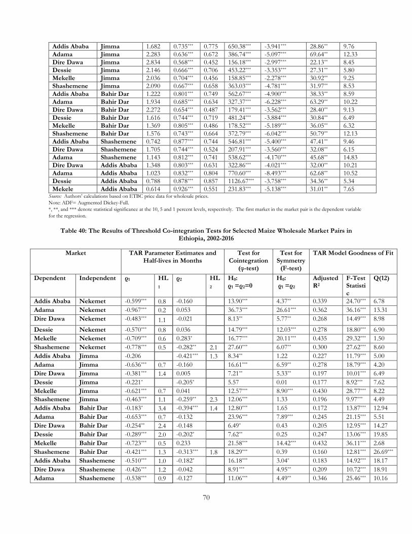
70

Addis Ababa Jimma 1.682 0.735*** 0.775 650.38*** -3.941*** 28.86** 9.76

Adama Jimma 2.283 0.636*** 0.672 386.74*** -5.097*** 69.64** 12.33

Dire Dawa Jimma 2.834 0.568*** 0.452 156.18*** -2.997*** 22.13** 8.45

Dessie Jimma 2.146 0.666*** 0.706 453.22*** -3.353*** 27.31** 5.80

Mekelle Jimma 2.036 0.704*** 0.456 158.85*** -2.278*** 30.92** 9.25

Shashemene Jimma 2.090 0.667*** 0.658 363.03*** -4.781*** 31.97** 8.53

Addis Ababa Bahir Dar 1.222 0.801*** 0.749 562.67*** -4.900*** 38.33** 8.59

Adama Bahir Dar 1.934 0.685*** 0.634 327.37*** -6.228*** 63.29** 10.22

Dire Dawa Bahir Dar 2.272 0.654*** 0.487 179.41*** -3.562*** 28.40** 9.13

Dessie Bahir Dar 1.616 0.744*** 0.719 481.24*** -3.884*** 30.84** 6.49

Mekelle Bahir Dar 1.369 0.805*** 0.486 178.52*** -5.189*** 36.05** 6.32

Shashemene Bahir Dar 1.576 0.743*** 0.664 372.79*** -6.042*** 50.79** 12.13

Addis Ababa Shashemene 0.742 0.877*** 0.744 546.81*** -5.400*** 47.41** 9.46

Dire Dawa Shashemene 1.705 0.744*** 0.524 207.91*** -3.560*** 32.08** 6.15

Adama Shashemene 1.143 0.812*** 0.741 538.62*** -4.170*** 45.68** 14.83

Dire Dawa Addis Ababa 1.348 0.803*** 0.631 322.86*** -4.021*** 32.00** 10.21

Adama Addis Ababa 1.023 0.832*** 0.804 770.60*** -8.493*** 62.68** 10.52

Dessie Addis Ababa 0.788 0.878*** 0.857 1126.67*** -3.758*** 34.36** 5.34

Mekele Addis Ababa 0.614 0.926*** 0.551 231.83*** -5.138*** 31.01** 7.65 Source: Authors’ calculations based on ETBC price data for wholesale prices.

Note: ADF= Augmented Dickey-Full.

*, **, and *** denote statistical significance at the 10, 5 and 1 percent levels, respectively. The first market in the market pair is the dependent variable

for the regression.

Table 40: The Results of Threshold Co-integration Tests for Selected Maize Wholesale Market Pairs in Ethiopia, 2002-2016

Market TAR Parameter Estimates and Half-lives in Months

Test for Cointegration

(φ-test)

Test for Symmetry

(F-test)

TAR Model Goodness of Fit

Dependent Independent ρ1 HL

1 ρ2 HL

2 H0: ρ1 =ρ2=0

H0: ρ1 =ρ2

Adjusted R2

F-Test Statistic

Q(12)

Addis Ababa Nekemet -0.599*** 0.8 -0.160 13.90*** 4.37** 0.339 24.70*** 6.78

Adama Nekemet -0.967*** 0.2 0.053 36.73*** 26.61*** 0.362 36.16*** 13.31

Dire Dawa Nekemet -0.483*** 1.1 -0.021 8.13** 5.77** 0.268 14.49*** 8.98

Dessie Nekemet -0.570*** 0.8 0.036 14.79*** 12.03*** 0.278 18.80*** 6.90

Mekelle Nekemet -0.709*** 0.6 0.283* 16.77*** 20.11*** 0.435 29.32*** 1.50

Shashemene Nekemet -0.778*** 0.5 -0.282** 2.1 27.60*** 6.07** 0.300 27.62*** 8.60

Addis Ababa Jimma -0.206 -0.421*** 1.3 8.34** 1.22 0.227 11.79*** 5.00

Adama Jimma -0.636*** 0.7 -0.160 16.61*** 6.59** 0.278 18.79*** 4.20

Dire Dawa Jimma -0.381*** 1.4 0.005 7.21** 5.33** 0.197 10.01*** 6.49

Dessie Jimma -0.221* -0.205* 5.57 0.01 0.177 8.92*** 7.62

Mekelle Jimma -0.621*** 0.7 0.041 12.57*** 8.90*** 0.430 28.77*** 8.22

Shashemene Jimma -0.463*** 1.1 -0.259** 2.3 12.06*** 1.33 0.196 9.97*** 4.49

Addis Ababa Bahir Dar -0.183* 3.4 -0.394*** 1.4 12.80*** 1.65 0.172 13.87*** 12.94

Adama Bahir Dar -0.653*** 0.7 -0.132 23.96*** 7.89*** 0.245 21.15*** 5.51

Dire Dawa Bahir Dar -0.254** 2.4 -0.148 6.49* 0.43 0.205 12.95*** 14.27

Dessie Bahir Dar -0.289*** 2.0 -0.202* 7.62** 0.25 0.247 13.06*** 19.85

Mekelle Bahir Dar -0.723*** 0.5 0.233 21.58*** 14.42*** 0.432 36.11*** 2.68

Shashemene Bahir Dar -0.421*** 1.3 -0.313*** 1.8 18.29*** 0.39 0.160 12.81*** 26.69***

Addis Ababa Shashemene -0.510*** 1.0 -0.182* 16.18*** 3.04* 0.183 14.92*** 18.17

Dire Dawa Shashemene -0.426*** 1.2 -0.042 8.91*** 4.95** 0.209 10.72*** 18.91

Adama Shashemene -0.538*** 0.9 -0.127 11.06*** 4.49** 0.346 25.46*** 10.16

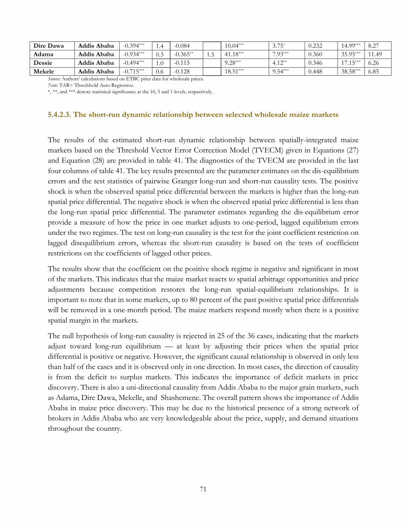
71

Dire Dawa Addis Ababa -0.394*** 1.4 -0.084 10.04*** 3.75* 0.232 14.99*** 8.27

Adama Addis Ababa -0.934*** 0.3 -0.365** 1.5 41.18*** 7.93*** 0.360 35.95*** 11.49

Dessie Addis Ababa -0.494*** 1.0 -0.115 9.28*** 4.12** 0.346 17.15*** 6.26

Mekele Addis Ababa -0.715*** 0.6 -0.128 18.51*** 9.54*** 0.448 38.58*** 6.85 Source: Authors’ calculations based on ETBC price data for wholesale prices.

Note: TAR= Threshhold Auto Regressive.

*, **, and *** denote statistical significance at the 10, 5 and 1 levels, respectively.

5.4.2.3. The short-run dynamic relationship between selected wholesale maize markets

The results of the estimated short-run dynamic relationship between spatially-integrated maize

markets based on the Threshold Vector Error Correction Model (TVECM) given in Equations (27)

and Equation (28) are provided in table 41. The diagnostics of the TVECM are provided in the last

four columns of table 41. The key results presented are the parameter estimates on the dis-equilibrium

errors and the test statistics of pairwise Granger long-run and short-run causality tests. The positive

shock is when the observed spatial price differential between the markets is higher than the long-run

spatial price differential. The negative shock is when the observed spatial price differential is less than

the long-run spatial price differential. The parameter estimates regarding the dis-equilibrium error

provide a measure of how the price in one market adjusts to one-period, lagged equilibrium errors

under the two regimes. The test on long-run causality is the test for the joint coefficient restriction on

lagged disequilibrium errors, whereas the short-run causality is based on the tests of coefficient

restrictions on the coefficients of lagged other prices.

The results show that the coefficient on the positive shock regime is negative and significant in most

of the markets. This indicates that the maize market reacts to spatial arbitrage opportunities and price

adjustments because competition restores the long-run spatial-equilibrium relationships. It is

important to note that in some markets, up to 80 percent of the past positive spatial price differentials

will be removed in a one-month period. The maize markets respond mostly when there is a positive

spatial margin in the markets.

The null hypothesis of long-run causality is rejected in 25 of the 36 cases, indicating that the markets

adjust toward long-run equilibrium — at least by adjusting their prices when the spatial price

differential is positive or negative. However, the significant causal relationship is observed in only less

than half of the cases and it is observed only in one direction. In most cases, the direction of causality

is from the deficit to surplus markets. This indicates the importance of deficit markets in price

discovery. There is also a uni-directional causality from Addis Ababa to the major grain markets, such

as Adama, Dire Dawa, Mekelle, and Shashemene. The overall pattern shows the importance of Addis

Ababa in maize price discovery. This may be due to the historical presence of a strong network of

brokers in Addis Ababa who are very knowledgeable about the price, supply, and demand situations

throughout the country.

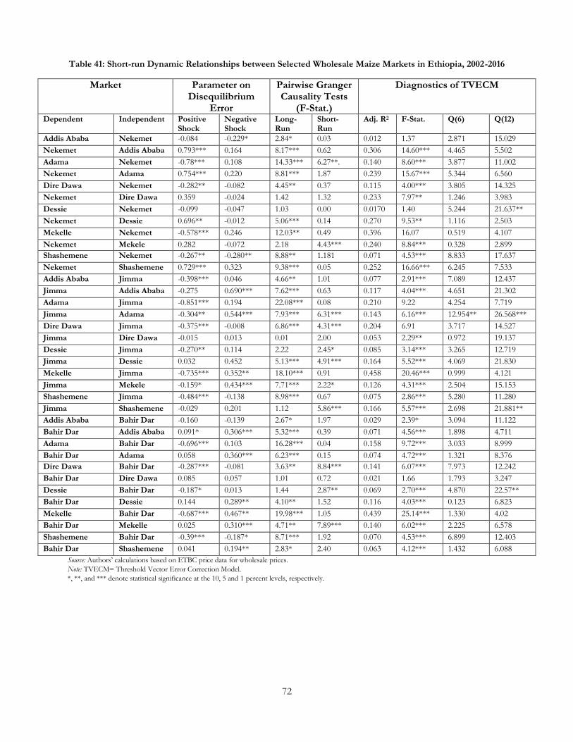
72

Table 41: Short-run Dynamic Relationships between Selected Wholesale Maize Markets in Ethiopia, 2002-2016

Market Parameter on Disequilibrium

Error

Pairwise Granger Causality Tests

(F-Stat.)

Diagnostics of TVECM

Dependent Independent Positive Shock

Negative Shock

Long-Run

Short-Run

Adj. R2 F-Stat. Q(6) Q(12)

Addis Ababa Nekemet -0.084 -0.229* 2.84* 0.03 0.012 1.37 2.871 15.029

Nekemet Addis Ababa 0.793*** 0.164 8.17*** 0.62 0.306 14.60*** 4.465 5.502

Adama Nekemet -0.78*** 0.108 14.33*** 6.27**. 0.140 8.60*** 3.877 11.002

Nekemet Adama 0.754*** 0.220 8.81*** 1.87 0.239 15.67*** 5.344 6.560

Dire Dawa Nekemet -0.282** -0.082 4.45** 0.37 0.115 4.00*** 3.805 14.325

Nekemet Dire Dawa 0.359 -0.024 1.42 1.32 0.233 7.97** 1.246 3.983

Dessie Nekemet -0.099 -0.047 1.03 0.00 0.0170 1.40 5.244 21.637**

Nekemet Dessie 0.696** -0.012 5.06*** 0.14 0.270 9.53** 1.116 2.503

Mekelle Nekemet -0.578*** 0.246 12.03** 0.49 0.396 16.07 0.519 4.107

Nekemet Mekele 0.282 -0.072 2.18 4.43*** 0.240 8.84*** 0.328 2.899

Shashemene Nekemet -0.267** -0.280** 8.88** 1.181 0.071 4.53*** 8.833 17.637

Nekemet Shashemene 0.729*** 0.323 9.38*** 0.05 0.252 16.66*** 6.245 7.533

Addis Ababa Jimma -0.398*** 0.046 4.66** 1.01 0.077 2.91*** 7.089 12.437

Jimma Addis Ababa -0.275 0.690*** 7.62*** 0.63 0.117 4.04*** 4.651 21.302

Adama Jimma -0.851*** 0.194 22.08*** 0.08 0.210 9.22 4.254 7.719

Jimma Adama -0.304** 0.544*** 7.93*** 6.31*** 0.143 6.16*** 12.954** 26.568***

Dire Dawa Jimma -0.375*** -0.008 6.86*** 4.31*** 0.204 6.91 3.717 14.527

Jimma Dire Dawa -0.015 0.013 0.01 2.00 0.053 2.29** 0.972 19.137

Dessie Jimma -0.270** 0.114 2.22 2.45* 0.085 3.14*** 3.265 12.719

Jimma Dessie 0.032 0.452 5.13*** 4.91*** 0.164 5.52*** 4.069 21.830

Mekelle Jimma -0.735*** 0.352** 18.10*** 0.91 0.458 20.46*** 0.999 4.121

Jimma Mekele -0.159* 0.434*** 7.71*** 2.22* 0.126 4.31*** 2.504 15.153

Shashemene Jimma -0.484*** -0.138 8.98*** 0.67 0.075 2.86*** 5.280 11.280

Jimma Shashemene -0.029 0.201 1.12 5.86*** 0.166 5.57*** 2.698 21.881**

Addis Ababa Bahir Dar -0.160 -0.139 2.67* 1.97 0.029 2.39* 3.094 11.122

Bahir Dar Addis Ababa 0.091* 0.306*** 5.32*** 0.39 0.071 4.56*** 1.898 4.711

Adama Bahir Dar -0.696*** 0.103 16.28*** 0.04 0.158 9.72*** 3.033 8.999

Bahir Dar Adama 0.058 0.360*** 6.23*** 0.15 0.074 4.72*** 1.321 8.376

Dire Dawa Bahir Dar -0.287*** -0.081 3.63** 8.84*** 0.141 6.07*** 7.973 12.242

Bahir Dar Dire Dawa 0.085 0.057 1.01 0.72 0.021 1.66 1.793 3.247

Dessie Bahir Dar -0.187* 0.013 1.44 2.87** 0.069 2.70*** 4.870 22.57**

Bahir Dar Dessie 0.144 0.289** 4.10** 1.52 0.116 4.03*** 0.123 6.823

Mekelle Bahir Dar -0.687*** 0.467** 19.98*** 1.05 0.439 25.14*** 1.330 4.02

Bahir Dar Mekelle 0.025 0.310*** 4.71** 7.89*** 0.140 6.02*** 2.225 6.578

Shashemene Bahir Dar -0.39*** -0.187* 8.71*** 1.92 0.070 4.53*** 6.899 12.403

Bahir Dar Shashemene 0.041 0.194** 2.83* 2.40 0.063 4.12*** 1.432 6.088

Source: Authors’ calculations based on ETBC price data for wholesale prices.

Note: TVECM= Threshold Vector Error Correction Model.

*, **, and *** denote statistical significance at the 10, 5 and 1 percent levels, respectively.

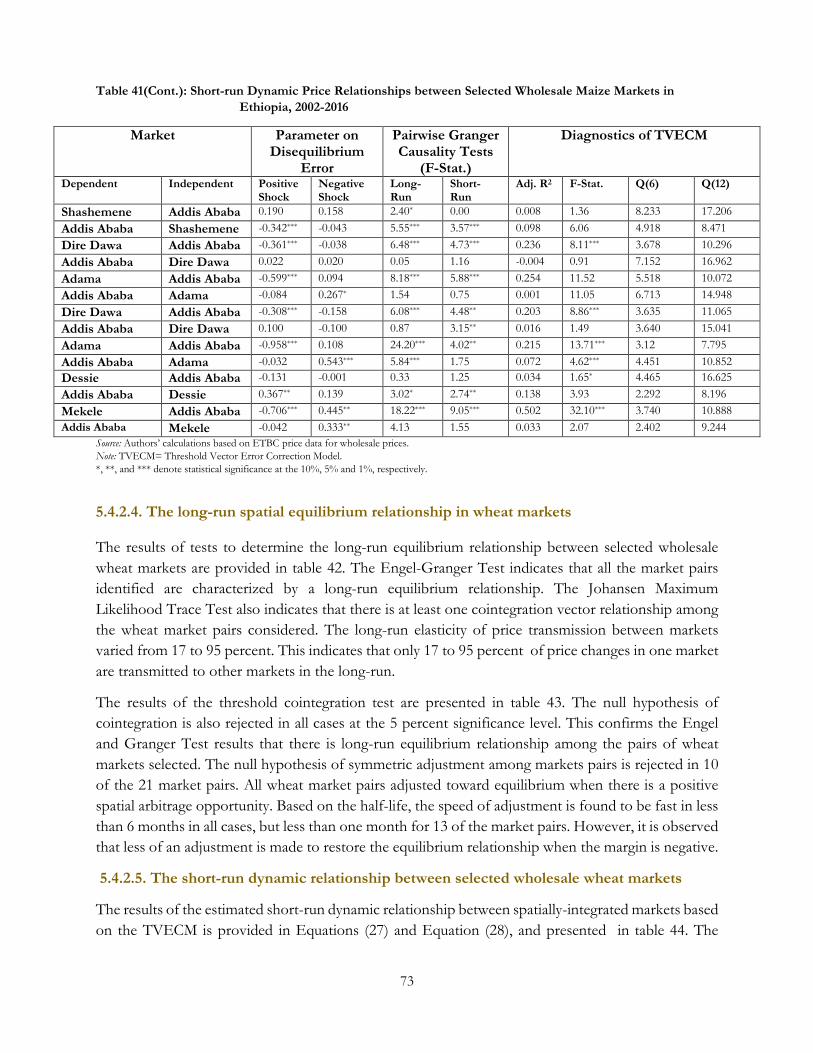
73

Table 41(Cont.): Short-run Dynamic Price Relationships between Selected Wholesale Maize Markets in

Ethiopia, 2002-2016


Error


(F-Stat.)



Negative Shock

Long-Run

Short-Run

Adj. R2 F-Stat. Q(6) Q(12)

Shashemene Addis Ababa 0.190 0.158 2.40* 0.00 0.008 1.36 8.233 17.206

Addis Ababa Shashemene -0.342*** -0.043 5.55*** 3.57*** 0.098 6.06 4.918 8.471

Dire Dawa Addis Ababa -0.361*** -0.038 6.48*** 4.73*** 0.236 8.11*** 3.678 10.296

Addis Ababa Dire Dawa 0.022 0.020 0.05 1.16 -0.004 0.91 7.152 16.962

Adama Addis Ababa -0.599*** 0.094 8.18*** 5.88*** 0.254 11.52 5.518 10.072

Addis Ababa Adama -0.084 0.267* 1.54 0.75 0.001 11.05 6.713 14.948

Dire Dawa Addis Ababa -0.308*** -0.158 6.08*** 4.48** 0.203 8.86*** 3.635 11.065

Addis Ababa Dire Dawa 0.100 -0.100 0.87 3.15** 0.016 1.49 3.640 15.041

Adama Addis Ababa -0.958*** 0.108 24.20*** 4.02** 0.215 13.71*** 3.12 7.795

Addis Ababa Adama -0.032 0.543*** 5.84*** 1.75 0.072 4.62*** 4.451 10.852

Dessie Addis Ababa -0.131 -0.001 0.33 1.25 0.034 1.65* 4.465 16.625

Addis Ababa Dessie 0.367** 0.139 3.02* 2.74** 0.138 3.93 2.292 8.196

Mekele Addis Ababa -0.706*** 0.445** 18.22*** 9.05*** 0.502 32.10*** 3.740 10.888

Addis Ababa Mekele -0.042 0.333** 4.13 1.55 0.033 2.07 2.402 9.244


Note: TVECM= Threshold Vector Error Correction Model.

*, **, and *** denote statistical significance at the 10%, 5% and 1%, respectively.

5.4.2.4. The long-run spatial equilibrium relationship in wheat markets

The results of tests to determine the long-run equilibrium relationship between selected wholesale

wheat markets are provided in table 42. The Engel-Granger Test indicates that all the market pairs

identified are characterized by a long-run equilibrium relationship. The Johansen Maximum

Likelihood Trace Test also indicates that there is at least one cointegration vector relationship among

the wheat market pairs considered. The long-run elasticity of price transmission between markets

varied from 17 to 95 percent. This indicates that only 17 to 95 percent of price changes in one market

are transmitted to other markets in the long-run.

The results of the threshold cointegration test are presented in table 43. The null hypothesis of

cointegration is also rejected in all cases at the 5 percent significance level. This confirms the Engel

and Granger Test results that there is long-run equilibrium relationship among the pairs of wheat

markets selected. The null hypothesis of symmetric adjustment among markets pairs is rejected in 10

of the 21 market pairs. All wheat market pairs adjusted toward equilibrium when there is a positive

spatial arbitrage opportunity. Based on the half-life, the speed of adjustment is found to be fast in less

than 6 months in all cases, but less than one month for 13 of the market pairs. However, it is observed

that less of an adjustment is made to restore the equilibrium relationship when the margin is negative.

5.4.2.5. The short-run dynamic relationship between selected wholesale wheat markets

The results of the estimated short-run dynamic relationship between spatially-integrated markets based

on the TVECM is provided in Equations (27) and Equation (28), and presented in table 44. The

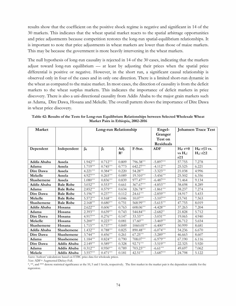
74

results show that the coefficient on the positive shock regime is negative and significant in 14 of the

30 markets. This indicates that the wheat spatial market reacts to the spatial arbitrage opportunities

and price adjustments because competition restores the long-run spatial-equilibrium relationships. It

is important to note that price adjustments in wheat markets are lower than those of maize markets.

This may be because the government is more heavily intervening in the wheat markets.

The null hypothesis of long-run causality is rejected in 14 of the 30 cases, indicating that the markets

adjust toward long-run equilibrium — at least by adjusting their prices when the spatial price

differential is positive or negative. However, in the short run, a significant causal relationship is

observed only in four of the cases and in only one direction. There is a limited short-run dynamic in

the wheat as compared to the maize market. In most cases, the direction of causality is from the deficit

markets to the wheat surplus markets. This indicates the importance of deficit markets in price

discovery. There is also a uni-directional causality from Addis Ababa to the major grain markets such

as Adama, Dire Dawa, Hosana and Mekelle. The overall pattern shows the importance of Dire Dawa

in wheat price discovery.

Table 42: Results of the Tests for Long-run Equilibrium Relationships between Selected Wholesale Wheat Market Pairs in Ethiopia, 2002-2016

Market Long-run Relationship Engel-Granger Test on

Residuals

Johansen Trace Test

Dependent Independent β0 β1 Adj. R2

F-Stat. ADF H0: r=0 vs Ha: r≥1

H0: r≤1 vs. Ha: r≥2

Addis Ababa Assela 1.942*** 0.712*** 0.809 796.38*** -5.897*** 57.755 7.278

Adama Assela 1.719*** 0.745*** 0.773 642.27*** -4.112*** 25.525 6.221

Dire Dawa Assela 4.221*** 0.384*** 0.220 54.28*** -3.323*** 21.038 4.996

Mekelle Assela 4.927*** 0.265*** 0.089 19.310*** -3.456*** 25.502 6.356

Shashemene Assela 1.080*** 0.836*** 0.839 977.47*** -6.487*** 71.464 9.134

Addis Ababa Bale Robe 3.032*** 0.553*** 0.661 367.67*** -4.853*** 38.698 8.289

Adama Bale Robe 2.852*** 0.579*** 0.634 326.78*** -1.861*** 38.237 7.274

Dire Dawa Bale Robe 5.196*** 0.237*** 0.112 24.61*** -2.859*** 18.917 5.433

Mekelle Bale Robe 5.572*** 0.168*** 0.046 10.07*** -3.107*** 23.741 7.563

Shashemene Bale Robe 2.168*** 0.680*** 0.751 568.99*** -5.615*** 47.755 8.019

Addis Ababa Hosana 2.622*** 0.606*** 0.763 608.06*** -4.428*** 37.263 7.204

Adama Hosana 2.393*** 0.639*** 0.743 544.84*** -2.682** 21.828 5.712

Dire Dawa Hosana 4.917*** 0.276*** 0.147 33.33*** -3.031*** 19.065 4.940

Mekelle Hosana 5.200*** 0.223*** 0.081 17.60*** -3.469*** 26.712 5.654

Shashemene Hosana 1.715*** 0.737*** 0.849 1060.05*** -6.400*** 50.999 8.681

Addis Ababa Shashemene 1.432*** 0.788*** 0.825 890.48*** -6.074*** 54.236 6.670

Dire Dawa Shashemene 3.744*** 0.456*** 0.261 67.25*** -3.289*** 46.663 8.607

Adama Shashemene 1.184*** 0.824*** 0.790 708.07*** -6.979*** 67.190 6.116

Dire Dawa Addis Ababa 2.149*** 0.589*** 0.328 92.71*** -3.519*** 22.325 5.920

Adama Addis Ababa 0.312*** 0.950*** 0.789 703.23*** -6.61*** 49.697 7.062

Mekele Addis Ababa 3.557*** 0.471*** 0.181 42.51*** -3.687*** 24.798 5.122 Source: Authors’ calculations based on ETBC price data for wholesale prices.

Note: ADF= Augmented Dickey-Full.

*, **, and *** denote statistical significance at the 10, 5 and 1 levels, respectively. The first market in the market pair is the dependent variable for the

regression.

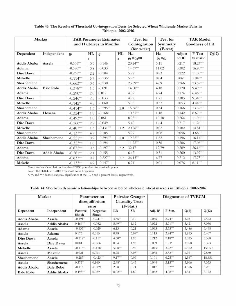
75

Table 43: The Results of Threshold Co-integration Tests for Selected Wheat Wholesale Market Pairs in Ethiopia, 2002-2016

Market TAR Parameter Estimates and Half-lives in Months

Test for Cointegration

(for φ-test)

Test for Symmetry

(F-test)

TAR Model Goodness of Fit

Dependent Independent ρ1 HL

1 ρ2 HL

2 H0: ρ1 =ρ2=0

H0: ρ1 =ρ2

Adjusted R2

F-Test Statistic

Q(12)

Addis Ababa Assela -0.536*** 0.9 -0.146 20.24*** 5.11 0.217 18.24***

Adama -0.580*** 0.8 -0.033 14.37*** 11.02 0.302 16.90***

Dire Dawa -0.266*** 2.2 -0.104 5.92 0.83 0.222 11.50***

Mekelle -0.114*** 5.7 -0.135* 5.93 0.04 0.061 5.04***

Shashemene -0.663*** 0.6 -0.230 23.69*** 4.69 0.266 23.52***

Addis Ababa Bale Robe -0.378*** 1.5 -0.091 14.00*** 4.18 0.120 9.49***

Adama -0.290*** 2.0 0.017 4.09 4.74 0.174 6.46***

Dire Dawa -0.246*** 2.5 -0.033 4.92 1.71 0.185 9.34***

Mekelle -0.142** 4.5 -0.060 5.06 0.57 0.053 4.44***

Shashemene -0.414*** 1.3 -0.295** 2.0 15.86*** 0.54 0.166 13.32***

Addis Ababa Hosana -0.324*** 1.8 -0.168* 10.35*** 1.18 0.142 8.67***

Adama -0.493*** 1.0 0.061 8.93*** 10.38 0.264 11.96***

Dire Dawa -0.266*** 2.2 -0.049 5.40 1.64 0.217 11.26***

Mekelle -0.407*** 1.3 -0.431*** 1.2 20.26*** 0.02 0.182 14.81***

Shashemene -0.137*** 4.7 -0.105 5.99* 0.08 0.056 4.68***

Addis Ababa Shashemene -0.521*** 0.9 -0.294*** 2.0 19.22*** 1.62 0.196 16.14***

Dire Dawa -0.323*** 1.8 -0.194 11.22*** 0.56 0.206 17.06***

Adama -0.872*** 0.3 -0.197** 3.2 32.17 12.79 0.289 26.16***

Dire Dawa Addis Ababa -0.281*** 2.1 -0.155 6.42* 0.51 0.260 13.97***

Adama -0.637*** 0.7 -0.227** 2.7 26.13*** 6.77 0.212 17.73***

Mekele -0.133*** 4.9 -0.147* 6.74* 0.01 0.076 6.11*** Source: Authors’ calculations based on ETBC price data for wholesale prices.

Note: HL=Half-Life; TAR= Threshold Auto Regressive

*, **, and *** denote statistical significance at the 10, 5 and 1 percent levels, respectively.

Table 44: Short-run dynamic relationships between selected wholesale wheat markets in Ethiopia, 2002-2016

Market Parameter on disequilibrium

error


(F-Stat.)



Negative Shock

LR SR Adj. R2 F-Stat. Q(6) Q(12)

Addis Ababa Assela -0.191** -0.241** 4.56** 0.10 0.036 2.74** 3.931 7.522

Assela Addis Ababa 0.466*** -0.082 5.69*** 1.12 0.092 5.71*** 5.421 8.056

Adama Assela -0.435*** -0.029 6.13 0.21 0.093 3.35*** 3.486 6.498

Assela Adama 0.173 0.016 0.78 3.09** 0.113 3.94*** 1.853 3.407

Dire Dawa Assela -0.212** -0.157 4.60** 1.95 0.212 7.18*** 2.025 6.388

Assela Dire Dawa 0.081 -0.066 0.54 1.93 0.039 1.93* 3.058 6.323

Mekelle Assela -0.118** -0.118 5.08*** 0.92 0.045 3.22** 6.372 15.050

Assela Mekelle -0.021 0.063 0.28 5.08** 0.038 2.82** 6.921 9.850

Shashemene Assela -0.287** -0.423*** 9.17*** 0.09 0.101 6.25*** 1.947 18.456

Assela Shashemene 0.375** 0.160 2.98* 0.43 0.044 3.15*** 3.906 7.335

Addis Ababa Bale Robe -0.115 -0.089 2.08 0.71 0.017 1.82*** 4.356 6.261

Bale Robe Addis Ababa 0.493*** 0.029 8.02*** 1.80 0.062 4.08*** 4.341 8.172

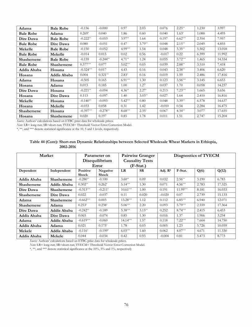
76

Adama Bale Robe -0.156 -0.000 0.97 2.03 0.076 2.25** 1.230 3.997

Bale Robe Adama 0.269* 0.040 1.86 0.60 0.040 1.63* 1.088 4.495

Dire Dawa Bale Robe -0.222** -0.053 3.97** 1.64 0.197 6.62*** 2.354 7.957

Bale Robe Dire Dawa 0.080 -0.051 0.47 3.79** 0.048 2.15** 2.049 4.855

Mekelle Bale Robe -0.150 -0.052 4.99*** 1.54 0.048 3.35** 5.502 13.018

Bale Robe Mekelle -0.014 0.015 0.02 0.56 -0.017 0.22 6.399 11.992

Shashemene Bale Robe -0.159 -0.244** 4.71** 1.24 0.055 3.72*** 1.465 14.334

Bale Robe Shashemene 0.377*** 0.077 5.02*** 0.03 0.039 2.88** 3.510 7.418

Addis Ababa Hosana -0.324*** 0.017 4.43 0.16 0.043 2.38** 3.406 6.620

Hosana Addis Ababa 0.004 0.321** 2.83* 0.16 0.019 1.59 2.486 17.816

Adama Hosana -0.505 0.165 6.91*** 1.30 0.123 3.56*** 3.145 6.653

Hosana Adama 0.013 0.185 1.00 1.27 0.037 1.70 0.058 14.237

Dire Dawa Hosana -0.221** -0.094 4.36** 2.27* 0.213 7.23*** 1.665 5.656

Hosana Dire Dawa 0.113 -0.097 1.40 3.03** 0.027 1.64 2.410 16.816

Mekelle Hosana -0.140** -0.093 5.42*** 0.80 0.048 3.39** 6.578 14.637

Hosana Mekelle -0.033 0.058 0.31 1.42 -0.010 0.54 2.284 16.475

Shashemene Hosana -0.397*** -0.278** 8.68*** 2.35* 0.067 4.34** 3.077 17.655

Hosana Shashemene 0.020 0.197 0.85 1.78 0.011 1.51 2.747 15.204


Note: LR= long-run; SR=short-run; TVECM= Threshold Vector Error Correction Model.

*, **, and *** denote statistical significance at the 10, 5 and 1 levels, respectively.

Table 44 (Cont): Short-run Dynamic Relationships between Selected Wholesale Wheat Markets in Ethiopia,

2002-2016


Error


(F-Stat.)



Negative Shock

LR SR Adj. R2 F-Stat. Q(6) Q(12)

Addis Ababa Shashemene -0.280** -0.100 3.60** 0.09 0.032 2.56** 3.190 6.783

Shashemene Addis Ababa 0.302** 0.262* 5.14*** 1.30 0.071 4.56*** 2.783 17.325

Dire Dawa Shashemene -0.313*** -0.211* 10.61*** 1.00 0.191 11.99*** 8.181 16.033

Shashemene Dire Dawa 0.022 -0.037 0.11 0.020 -0.020 0.07 2.739 15.133

Adama Shashemene -0.662*** 0.003 13.28*** 1.12 0.112 6.85*** 6.940 12.071

Shashemene Adama 0.253* 0.238* 5.06*** 2.20 0.093 5.79*** 2.559 17.364

Dire Dawa Addis Ababa -0.242** -0.189 5.38*** 3.15** 0.252 8.74*** 2.415 6.453

Addis Ababa Dire Dawa 0.065 -0.074 0.85 1.30 0.016 1.37 1.906 3.234

Adama Addis Ababa -0.619*** -0.060 14.14*** 1.57 0.118 7.22*** 7.664 14.750

Addis Ababa Adama 0.021 0.175* 1.78 0.03 0.005 1.23 5.726 10.059

Mekele Addis Ababa -0.116* -0.199* 6.03*** 1.60 0.062 4.07*** 4.671 11.330

Addis Ababa Mekele 0.044 -0.034 0.42 0.93 -0.004 0.81 5.473 8.773


Note: LR= long-run; SR=short-run; TVECM= Threshold Vector Error Correction Model.

*, **, and *** denote statistical significance at the 10%, 5% and 1%, respectively

77

6. Conclusions and policy implications

6.1 Conclusions

The temporal and spatial market performance of the maize and wheat markets in Ethiopia are

analyzed based on a rapid market appraisal, as well as on statistical and econometric analyses of

historical monthly prices (2001-2016) collected for different markets and market levels.

The overall results indicate that the maize and wheat markets are well integrated in the long run, but

that price transmission among some markets is inefficient. There is a significant long-run spatial

equilibrium relationship between maize and wheat markets. However, there is incomplete price

transmission and asymmetric price adjustments. There are excessive upward and downward

movements in the spatial gross marketing margins. Thus, the spatial margins are very volatile,

making inter-regional grain trade risky.

Although markets are integrated in the long run, there is significant unpredictability in wheat and

maize prices, implying a high risk for the value chain actors. There are slight upward movements in

maize and wheat prices at all levels, however there is significant unpredictability in maize and wheat

prices. This makes spot market temporal and spatial arbitrages very risky. For example, in the case of

maize markets about 6 to 33 percent (at the producer level), 0 to 72 percent (at the wholesale level)

and 2 to 45 percent (at the retail level) of the overall maize price fluctuations are explained by

unpredictable, random price movements. The corresponding figures in the case of wheat are 0 to 27

percent (at the producer level), 1 to 27 percent (at the wholesale level) and 0 to 46 (at the retail

level).

In addition, maize and wheat price volatility have been increasing more in recent years. High and

increasing volatility limits maize and wheat market transactions as market actors avoid risks. This

decreases the availability of maize and wheat both temporally and spatially. Furthermore, the high

risk (given the non-existence of efficient mechanisms to insure price risk) would discourage

necessary investments in maize and wheat production, as well as along the value chains. This

presents a significant bottleneck to the agricultural transformation agenda to improve smallholder

adoption of modern agricultural inputs and increase commercialization.

The incentives for the private sector to invest in storage facilities are limited. There is significant

seasonality for maize and wheat prices in different markets and at different value chain nodes, which

presents business opportunities for storage. However, the implied storage periods required between

the seasonal low and high appear to be very long (5 to 10 months) for both maize and wheat.

Furthermore, holding maize and wheat stocks does not provide sufficient incentives, given their very

low mean and highly volatile monthly returns. There are excessive downward and upward

movements in actual prices and returns which are not explained by the costs of storage in several

markets and at different market levels.

78

6.2 Policy Implications

Implications for Policy Options and Actions

The findings and conclusions of the study support the following proposed policy options and

actions:

1. Reduce price unpredictability through clearer policy directions and transparent information. An important

priority area is the necessity of improving the spatial efficiency of cereal marketing and

private sector investment in grain storage. This would help to reduce price unpredictability

and volatility. Under the current conditions, there are few incentives to hold wheat and

maize for storage. Likewise, there is not much incentive for the private sector to invest in

storage facilities. Greater transparency can help to reduce uncertainties faced by value-chain

actors. In particular, greater transparency is required with regard to the level of government

domestic grain procurement; pricing and distribution; grain imports; the timing and release

of imported grain in the market; the price at which it will be sold; and information on the

overall level of stock in the country. This will in turn help reduce price volatility in the short

term — and increase private sector investment in cereal markets. Overall, predictable

government policies that promote the participation of the private sector in grain trade and

storage will generally decrease price volatility.

2. Establish an agricultural market information system. Asymmetric price and production information

and a lack of clarity about price discovery significantly contributes to price and market

uncertainties. It is important to improve the reliability and accuracy of data so that the

government and key relevant institutions can make better policies and procurement

decisions. There is a need also to identify an institution at which a market information

system can be established to regularly collect and analyze production and price data, and

improve data reliability, timeliness and frequency. Before such a MIS is established, though,

a detailed assessment will be required to assess its value to key stakeholders, as well as their

willingness to fund and sustain such a system. This could entail establishing a new institution

or capacity building at existing institutions engaged in the provision of MIS, such as the CSA

or ETBC.

3. Reform the tax policy based on grain stocks alone. Arbitrary tax enforcement based on grain stocks

held by traders and wholesale distributors at a given time — and not considering their

turnover — creates huge disincentives for traders and wholesalers to engage in temporal

arbitrage. These are important value chain actors in grain storage and distribution, linking

producers to the markets, thereby enabling the movement of grain from surplus producing

areas to deficit areas. The tax should not be based on output alone. Rather, it should be

clearly enforced in a consistent manner.

4. Reassess the real needs for storage and the different types of storage technologies required at various market

levels. This includes clearly identifying the objective of storage at the farm, cooperative,

79

union, processor, wholesaler and retailer levels. The objective for storage facilities could be

for aggregation or arbitrage, or simply to minimize post-harvest losses. Each cause would

have different implications on the required capacity and investments. For example, improved

access to low-cost hermetic bags at the household level can greatly minimize losses. If the

cooperative’s objective is simply to aggregate or bulk and sell quickly, then other

technologies, such as this large volume storage hermetic cocoons or temporary sheds may be

required. This may be the case for some primary cooperatives. However, if it is for storing

large volumes for arbitrage which would require longer holding periods, then building a

bigger storage facility with good aeration and higher standards would be required. This is

often the case for cooperative unions.

5. Encourage independent certification of grain quality and enforce grain standards. This would help to:

encourage producers to increase the quality of the grain that they sell to millers and other

buyers; minimize cheating in the grain marketing; reward the adoption of and investments in

quality enhancing technologies and best practices; and strengthen food safety. In addition,

investments in post-harvest conditioning to make maize and wheat storable commodities

increases the overall quality of the grain being marketed. As such, it can also create job

opportunities for youth in the rural sector.

6. Improve the capacity of primary cooperatives to become effective aggregators for the cooperative unions.

Cooperatives remain a key vehicle to linking smallholder farmers to processors and other

market buyers. Turning primary cooperatives into effective aggregators for cooperative

unions and increasing the marketing potential requires strengthening the managerial capacity

of cooperatives. This would include building their agribusiness leadership skills, hiring

professional managers, and fostering trust with their members.

7. Reconsider the timing and the scaling-up process of public investments in the cooperative warehouse facilities.

Considering points (4) and (6), and given the negligible amount of marketed output being

sold by the primary cooperatives, the lack of trust, and the current low capacity of

cooperatives’ marketing function, building more warehouses will not guarantee a substantial

increase in farmers’ sales and/or the storing of grain through primary cooperatives.

8. Improve the coordination and planning among grain importing entities to utilize the existing public storage

system optimally. There is a need to improve coordination and planning among the key entities

involved in grain importation to increase the swapping of public warehouses facilities and

synchronize importation of grain in the country to avoid the simultaneous arrival of large

quantities of grain into the local market.

9. Increasing the proportion of cash-based transfers for PSNP beneficiaries and for aid recipients by other

organizations in responding to food emergency situations should be taken cautiously considering the specific

local conditions. First, the results indicate that maize and wheat markets are spatially

80

integrated in the long-run, which supports the movement of grain from surplus to deficit

areas. Although this result would generally support increasing cash transfers by the PSNP

program, the long-run elasticity of price transmission estimates indicate that the long-run

price transmissions are less than complete for some markets and the price transmission is

asymmetric. Furthermore, there are limited short-term price dynamics among the spatially-

linked markets. This indicates inefficiencies in wheat and maize price transmission — despite

the wheat and maize markets being integrated.

Second, wheat wholesale and retail prices are highly volatile, with a large component of the

volatility being unpredictable in some markets at retail, wholesale and producer levels. The

price analyses indicate that there is limited commercial incentive for the private sector to

engage in grain storage. The implication is that the complete reliance on markets and the

private sector to respond effectively under emergency situations is not advisable. There

needs to a targeted approach, accompanied by careful and close monitoring. Ideally this

could entail using more cash responses during the harvest time, but in-kind food transfers

during the lean period. But there are significant operational constraints for PSNP to

implement such time sensitive responses. Given the weak storage system under the current

market conditions, relying heavily on the market to respond to emergency situations is also

not advisable.

Third, the high unpredictability of price fluctuations imply that the purchasing power of cash

recipients is also uncertain. The complete adoption of cash transfer as the sole mode of

payment assumes that products are available in the market and that the private sector and

the market have adequate capacity to respond. Therefore, in the short-run it is advisable to

maintain a reasonable mix of in-kind transfers and cash transfers in the PSNP. If cash is

used in deficit areas, one would need a reliable trade network, storage capability, a market

information system, and infrastructure based on regular market and price monitoring. An

assessment to make timely adjustments in the amount of cash transfers would also be

required. Further price and market analysis at the local level would be required for the PSNP

and other humanitarian entities to inform them about where and when to use cash or food

transfers.

Lastly, to provide clearer and location-specific evidence-based guidance for the PSNP

program on cash vs food transfers and guidelines on policy negotiations, further analysis

regarding food availability and prices using more local specific data combined with LSMS

data to showing market position of households, and focusing on the lowland region where

the PSNP program is struggling to implement cash-based transfers, are required, In

addition, it is also important to conduct further analysis on the extent the random

component of price volatility is related to policy, procurement, lack of market information

81

and climatic shocks, and to consider other analyses16 that point more toward moving for

cash transfers.

V. Areas for Further Research

The following findings of the paper require further research before clear recommendations can be

made:

(1) Evaluate how much subsidized wheat is sold in the open market, and how this affects the

competitiveness of the local industries. This would also require finding ways to improve the

effective targeting of assistance to poor households, as well as better targeting of the

locations requiring food or cash assistance.

(2) The government may wish to consider and evaluate the impact of the wheat subsidy on

producers and the local market. There is a need to evaluate the level and extent of market

distortions created by the wheat subsidy to reform its targeting and cost effectiveness. This

would require a detailed analysis because such a distortion makes local prices relatively high,

thereby affecting the industry’s competitiveness. A related question is: Who is the

government really subsidizing? Poor and rich consumers alike, as well as foreign producers?

(3) Consider producer price support interventions. This will require detailed, regular

production cost data (enterprise budgeting) collection. However, it can greatly help the

government to know when it is necessary to intervene in the market, and at what price. It

can also help to inform farmers ahead of time about the expected minimum price so that

they can plan their production accordingly.

(4) Ways of strengthening the capacity, governance and the effective management of

cooperatives. Primary and union cooperatives present a useful platform to aggregate from

smallholder producers, who as a whole, dominate total cereal production in Ethiopia.

Improving the capacity of cooperatives to become effective aggregators — and increasing

smallholder market participation — is essential to achieving agricultural transformation and

commercialization.

(5) Is the export ban on maize trade still necessary? When the price of maize is depressed

due to over-production, exports might be one option to overcome this problem, along with

other considerations pertaining to the government’s price support options.

16 Ruth Hill and Habtamu Fuje (2017), What is the impact of drought on prices? Evidence from Ethiopia.

82

References

Ahmed, Raisuddin. 1988. “Pricing Principles and Public Intervention in Domestic

Markets.” In Agricultural Price Policy for Developing Countries , edited by John W. Mellor and

Raisuddin Ahmed, 55-80. Baltimore, Maryland: The Johns Hopkins University Press.

Ahmed, Raisuddin and John W. Mellor. 1988. “Agricultural Price Policy: The Context and

the Approach.” In Agricultural Price Policy for Developing Countries, edited by John W. Mellor and

Raisuddin Ahmed, 1-10.. Baltimore, Maryland: The Johns Hopkins University Press.

Barrett, C.B., and J.R. Li. 2002. “Distinguishing between Equilibrium and Integration in

Spatial Price Analysis.” American Journal of Agriculatual Economics 84: 292–307.

Bekele, G. 2002. “The Role of the Ethiopian Grain Trade Enterprise in Price Policy. In

Agriculture Technology Diffusion and Price Policy in Addis Ababa”. Proceedings of a Policy Forum in Addis Ababa: 2020 Vision Network for East Africa Report 1. Addis Ababa: Ethiopian Development Research Institute (Addis Ababa) and International Food Policy Research Institute (Washington DC).

Brorsen, B. Wade, Jean-Paul Chavas, and Warren R. Grant. 1987. “A Market Equilibrium

Analysis of the Impact of Risk on the U.S.A. Rice Industry.” American Journal of Agricultural

Economics 69: 733-739.

Myers, Robert. J. 2013. “Evaluating the Effectiveness of Inter-regional Trade and Storage

in Malawi’s Private Sector Maize Markets.” Food Policy 41: 75–84.

Delgado, Christopher. 1986. “A Variance Component Approach to Food Grain Market

Integration in Northern Nigeria.” American Journal of Agricultural Economies 68: 970–979.

Dickey, David A. and Wayne A. Fuller. 1979. “Distribution of the Estimators for

Autoregressive Time Series with a Unit Root. Journal of American Statistical Association 74: 427–

431.

Engle, Robert A. and C.W.J. Granger. 1987. “Cointegration and Error Correction:

Representation, Estimation and Testing.” Econometrica 55: 251–276.

Ethiopia, Central Statistics Agency. 2012a. Report on the 2010/2011 Household Income and

Expenditure Survey. Addis Ababa. Government of Ethiopia.

CSA. 2012b. “Report on Area and Production of Major Crops. Ethiopian Agricultural

Sample Survey Private Peasant Holdings.” Meher Season (2011/12 (2004 E.C.) – Volume I.

Statistical Bulletin. Addis Ababa: Central Statistical Agency.

83

Fafchamps, Marcel. 1992. “Cash Crop Production, Food Price Volatility, and Rural

Market Integration in the Third World.” American Journal of Agricultural Economies 74: 90–99.

Faminow, Merle D. and Bruce Benson. 1990. “Integration of Spatial Markets.” American

Journal of Agricultural Economies 72: 49–62.

FAO (2011). “Price Volatility in Food and Agricultural Markets” Policy Responses”.

http://www.fao.org/fileadmin/templates/est/Volatility/Interagency_Report_to_the_G20_

on_Food_Price_Volatility.pdf.

Goodwin, Barry K. and Ted C. Schroeder. 1991. “Cointegration Tests and Spatial Price

Linkages in Regional Cattle Markets.” American Journal of Agricultural Economies 73: 452–464.

Gurmu, M., Meyer, F. and Hassan R. “Modelling Price Formation and Dynamics in the

Ethiopian Maize Market.” Journal of Agricultural Science and Technology 18:1439-1452.

Heytens, Paul J. 1986. “Testing Market Integration.” Food Research Institute Studies 20: 25–41.

Hill, Ruth and Fuje, Habtamu (2017). “What is the impact of drought on prices? Evidence from Ethiopia”. World Bank.

Kohls, Richard L. and Joseph N. Uhl. 1990. Marketing of Agricultural Products. NY:

Macmillan.

Minten, B., D. Stife, and S. Tamru. 2014. “Structural Transformation of Cereal Markets

in Ethiopia.” The Journal of Development Studies. 50 (5) :611-629.

Negassa, A. and R. Meyers. 2007. “Estimating Policy Effects on Spatial Market

Efficiency: An Extension of the Parity Bound Model.” American Journal of Agricultural

Economics 89(2): 380-352.

Park, A., H. Jin, S. Rozelle, and J. Huang. 2002. Market Emergence and Transition:

Arbitrage, Transaction Costs, and Autarky in China’s Grain Markets.” American Journal of

Agricultural Economics 84: 67-82.

Pick, Daniel H., Jeffrey Karrenbrock and Hoy F. Carman. 1990. “Price Asymmetry and

Marketing Margin Behavior: An Example for California- Arizona Citrus.” Agribusiness 6: 75-

84.

Rashid, R. and A. Negassa. 2011. “Policies and Performance of Ethiopian Cereal Markets.”

Ethiopian Strategy Support Program II. ESSP II Working Paper 21, IFPRI, Washington,

DC.

http://www.fao.org/fileadmin/templates/est/Volatility/Interagency_Report_to_the_G20_on_Food_Price_Volatility.pdf

http://www.fao.org/fileadmin/templates/est/Volatility/Interagency_Report_to_the_G20_on_Food_Price_Volatility.pdf

84

Rashid, S. and S. Lemma. 2011. “Strategic Grain Reserves in Ethiopia: Institutional Design

and Operational Performance.” IFPRI Discussion Paper 01054. IFPRI, Washington, DC.

Ravallion, Martin. 1986. Testing Market Integration. American Journal of Agricultural Economics.

68: 102-109.

Sahn, David E., and Christopher Delgado. 1989. “The Nature and Implications for Market

Interventions of Seasonal Food Price Variability.” In Seasonal Variability in Third World

Agriculture: The Consequences for Food Security. 179–194. Baltimore, Maryland: The Johns

Hopkins University Press.

Southworth, V. Roy, William O. Jones and Scott R. Pearson. 1979. “Food Marketing in

Atebubu District, Ghana.” Food Research Institute Studies 17: 157–195.

Timmer, C. Peter. 1987..The relationship between price policy and food marketing". In

Food policy: Integrating supply, distribution, and consumption, edited by J. Gittinger, Joanne Leslie

Price, and Caroline Hoisington, 293–303. Baltimore, Maryland: The Johns Hopkins

University Press.

Tamru, S. 2013. “Spatial Integration of Cereal Markets in Ethiopia. Ethiopian Strategy Support

Program II.” ESSP II Working Paper 56. IFPRI, Washington, DC.

Timmer, C. Peter. 1987. “Price Policy and the Political Economy of Markets. In

Food Policy: Integrating Supply, Distribution, and Consumption, edited by J. Gittinger, Joanne Leslie

Price, and Caroline Hoisington, 264–276. Baltimore, Maryland.

Tomek, William G., and Kenneth 1. Robinson. 1991. Agricultural Product Prices.

Ithaca NY: Cormell University Press.

Tschirley, D.L. 1995. “Using Microcomputer Spreadsheets for Spatial and Temporal

Price Analysis: An Application to Rice and Maize in Ecuador.” In Prices, Products and People:

Analyzing Agricultural Markets in Developing Countries, edited by Gregory J. Scott, 277-300.

International Potato Center. Boulder, Colorado: Lynne Rienner Publishers, Inc.

Von Braun, J. and Olofinbiyi, T. 2007. “Famine and Food Security in Ethiopia.” In

Food Policy for Developing Countries: The Role of Government in the Global Food System, edited by P.

Pinstrup-Andersen and F. Cheng, 1–11. Ithaca, NY: Cornell University.

World Bank. 2016. “Food Price Stabilization South Asia. Impact of National Policies and

Implications for a Regional Approach.”

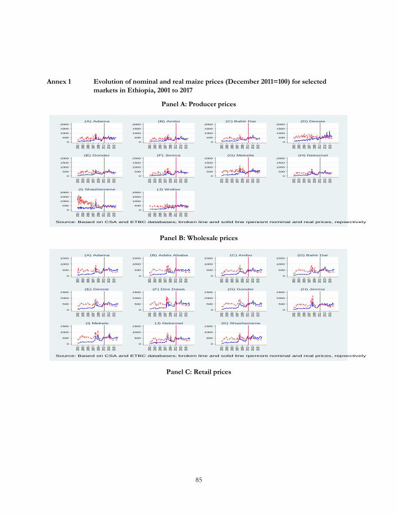
85

Annex 1 Evolution of nominal and real maize prices (December 2011=100) for selected

markets in Ethiopia, 2001 to 2017

Panel A: Producer prices

Panel B: Wholesale prices

Panel C: Retail prices

0

500

1000

1500

2000

2001

2003

2005

2007

2009

2011

2013

2015

(A) Adama

0

500

1000

1500

2000

2001

2003

2005

2007

2009

2011

2013

2015

(B) Ambo

0

500

1000

1500

2000

2001

2003

2005

2007

2009

2011

2013

2015

(C) Bahir Dar

0

500

1000

1500

2000

2001

2003

2005

2007

2009

2011

2013

2015

(D) Dessie

0

500

1000

1500

2000

2001

2003

2005

2007

2009

2011

2013

2015

(E) Gonder

0

500

1000

1500

2000

2001

2003

2005

2007

2009

2011

2013

2015

(F) Jimma

0

500

1000

1500

2000

2001

2003

2005

2007

2009

2011

2013

2015

(G) Mekelle

0

500

1000

1500

2000

2001

2003

2005

2007

2009

2011

2013

2015

(H) Nekemet

0

500

1000

1500

2000

2001

2003

2005

2007

2009

2011

2013

2015

(I) Shashemene

0

500

1000

1500

2000

2001

2003

2005

2007

2009

2011

2013

2015

(J) Woliso

Source: Based on CSA and ETBC databases; broken line and solid line rperesnt nominal and real prices, repsectively

0

500

1000

1500

2001

2003

2005

2007

2009

2011

2013

2015

(A) Adama

0

500

1000

1500

2001

2003

2005

2007

2009

2011

2013

2015

(B) Addis Ababa

0

500

1000

1500

2001

2003

2005

2007

2009

2011

2013

2015

(C) Ambo

0

500

1000

1500

2001

2003

2005

2007

2009

2011

2013

2015

(D) Bahir Dar

0

500

1000

1500

2001

2003

2005

2007

2009

2011

2013

2015

(E) Dessie

0

500

1000

1500

2001

2003

2005

2007

2009

2011

2013

2015

(F) Dire Dawa

0

500

1000

1500

2001

2003

2005

2007

2009

2011

2013

2015

(G) Gonder

0

500

1000

1500

2001

2003

2005

2007

2009

2011

2013

2015

(H) Jimma

0

500

1000

1500

2001

2003

2005

2007

2009

2011

2013

2015

(I) Mekele

0

500

1000

1500

2001

2003

2005

2007

2009

2011

2013

2015

(J) Nekemet

0

500

1000

1500

2001

2003

2005

2007

2009

2011

2013

2015

(K) Shashemene


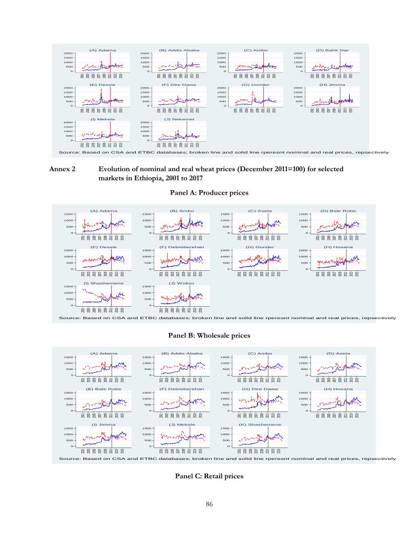
86

Annex 2 Evolution of nominal and real wheat prices (December 2011=100) for selected

markets in Ethiopia, 2001 to 2017

Panel A: Producer prices

Panel B: Wholesale prices

Panel C: Retail prices

0

500

1000

1500

2000

2001

2003

2005

2007

2009

2011

2013

2015

(A) Adama

0

500

1000

1500

2000

2001

2003

2005

2007

2009

2011

2013

2015

(B) Addis Ababa

0

500

1000

1500

2000

2001

2003

2005

2007

2009

2011

2013

2015

(C) Ambo

0

500

1000

1500

2000

2001

2003

2005

2007

2009

2011

2013

2015

(D) Bahir Dar

0

500

1000

1500

2000

2001

2003

2005

2007

2009

2011

2013

2015

(E) Dessie

0

500

1000

1500

2000

2001

2003

2005

2007

2009

2011

2013

2015

(F) Dire Dawa

0

500

1000

1500

2000

2001

2003

2005

2007

2009

2011

2013

2015

(G) Gonder

0

500

1000

1500

2000

2001

2003

2005

2007

2009

2011

2013

2015

(H) Jimma

0

500

1000

1500

2000

2001

2003

2005

2007

2009

2011

2013

2015

(I) Mekele

0

500

1000

1500

2000

2001

2003

2005

2007

2009

2011

2013

2015

(J) Nekemet


0

500

1000

1500

2001

2003

2005

2007

2009

2011

2013

2015

(A) Adama

0

500

1000

1500

2001

2003

2005

2007

2009

2011

2013

2015

(B) Ambo

0

500

1000

1500

2001

2003

2005

2007

2009

2011

2013

2015

(C) Asela

0

500

1000

1500

2001

2003

2005

2007

2009

2011

2013

2015

(D) Bale Robe

0

500

1000

1500

2001

2003

2005

2007

2009

2011

2013

2015

(E) Dessie

0

500

1000

1500

2001

2003

2005

2007

2009

2011

2013

2015

(F) Debreberehan

0

500

1000

1500

2001

2003

2005

2007

2009

2011

2013

2015

(G) Gonder

0

500

1000

1500

2001

2003

2005

2007

2009

2011

2013

2015

(H) Hosana

0

500

1000

1500

2001

2003

2005

2007

2009

2011

2013

2015

(I) Shashemene

0

500

1000

1500

2001

2003

2005

2007

2009

2011

2013

2015

(J) Woliso


0

500

1000

1500

2001

2003

2005

2007

2009

2011

2013

2015

(A) Adama

0

500

1000

1500

2001

2003

2005

2007

2009

2011

2013

2015

(B) Addis Ababa

0

500

1000

1500

2001

2003

2005

2007

2009

2011

2013

2015

(C) Ambo

0

500

1000

1500

2001

2003

2005

2007

2009

2011

2013

2015

(D) Asela

0

500

1000

1500

2001

2003

2005

2007

2009

2011

2013

2015

(E) Bale Robe

0

500

1000

1500

2001

2003

2005

2007

2009

2011

2013

2015

(F) Debreberehan

0

500

1000

1500

2001

2003

2005

2007

2009

2011

2013

2015

(G) Dire Dawa

0

500

1000

1500

2001

2003

2005

2007

2009

2011

2013

2015

(H) Hosana

0

500

1000

1500

2001

2003

2005

2007

2009

2011

2013

2015

(I) Jimma

0

500

1000

1500

2001

2003

2005

2007

2009

2011

2013

2015

(J) Mekele

0

500

1000

1500

2001

2003

2005

2007

2009

2011

2013

2015

(K) Shashemene


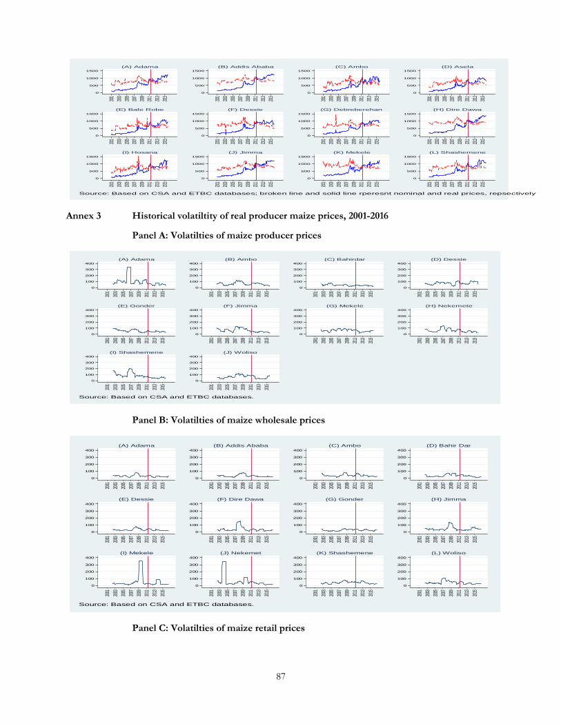
87

Annex 3 Historical volatiltity of real producer maize prices, 2001-2016

Panel A: Volatilties of maize producer prices

Panel B: Volatilties of maize wholesale prices

Panel C: Volatilties of maize retail prices

0

500

1000

1500

2001

2003

2005

2007

2009

2011

2013

2015

(A) Adama

0

500

1000

1500

2001

2003

2005

2007

2009

2011

2013

2015

(B) Addis Ababa

0

500

1000

1500

2001

2003

2005

2007

2009

2011

2013

2015

(C) Ambo

0

500

1000

1500

2001

2003

2005

2007

2009

2011

2013

2015

(D) Asela

0

500

1000

150020

01

2003

2005

2007

2009

2011

2013

2015

(E) Bale Robe

0

500

1000

1500

2001

2003

2005

2007

2009

2011

2013

2015

(F) Dessie

0

500

1000

1500

2001

2003

2005

2007

2009

2011

2013

2015

(G) Debreberehan

0

500

1000

1500

2001

2003

2005

2007

2009

2011

2013

2015

(H) Dire Dawa

0

500

1000

1500

2001

2003

2005

2007

2009

2011

2013

2015

(I) Hosana

0

500

1000

1500

2001

2003

2005

2007

2009

2011

2013

2015

(J) Jimma

0

500

1000

1500

2001

2003

2005

2007

2009

2011

2013

2015

(K) Mekele

0

500

1000

1500

2001

2003

2005

2007

2009

2011

2013

2015

(L) Shashemene


0

100

200

300

400

2001

2003

2005

2007

2009

2011

2013

2015

(A) Adama

0

100

200

300

400

2001

2003

2005

2007

2009

2011

2013

2015

(B) Ambo

0

100

200

300

400

2001

2003

2005

2007

2009

2011

2013

2015

(C) Bahirdar

0

100

200

300

400

2001

2003

2005

2007

2009

2011

2013

2015

(D) Dessie

0

100

200

300

400

2001

2003

2005

2007

2009

2011

2013

2015

(E) Gonder

0

100

200

300

400

2001

2003

2005

2007

2009

2011

2013

2015

(F) Jimma

0

100

200

300

400

2001

2003

2005

2007

2009

2011

2013

2015

(G) Mekele

0

100

200

300

400

2001

2003

2005

2007

2009

2011

2013

2015

(H) Nekemete

0

100

200

300

400

2001

2003

2005

2007

2009

2011

2013

2015

(I) Shashemene

0

100

200

300

400

2001

2003

2005

2007

2009

2011

2013

2015

(J) Woliso

Source: Based on CSA and ETBC databases.

0

100

200

300

400

2001

2003

2005

2007

2009

2011

2013

2015

(A) Adama

0

100

200

300

400

2001

2003

2005

2007

2009

2011

2013

2015

(B) Addis Ababa

0

100

200

300

400

2001

2003

2005

2007

2009

2011

2013

2015

(C) Ambo

0

100

200

300

400

2001

2003

2005

2007

2009

2011

2013

2015

(D) Bahir Dar

0

100

200

300

400

2001

2003

2005

2007

2009

2011

2013

2015

(E) Dessie

0

100

200

300

400

2001

2003

2005

2007

2009

2011

2013

2015

(F) Dire Dawa

0

100

200

300

400

2001

2003

2005

2007

2009

2011

2013

2015

(G) Gonder

0

100

200

300

400

2001

2003

2005

2007

2009

2011

2013

2015

(H) Jimma

0

100

200

300

400

2001

2003

2005

2007

2009

2011

2013

2015

(I) Mekele

0

100

200

300

400

2001

2003

2005

2007

2009

2011

2013

2015

(J) Nekemet

0

100

200

300

400

2001

2003

2005

2007

2009

2011

2013

2015

(K) Shashemene

0

100

200

300

400

2001

2003

2005

2007

2009

2011

2013

2015

(L) Woliso


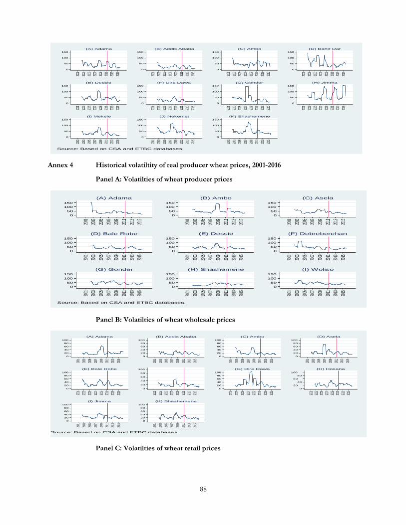
88

Annex 4 Historical volatiltity of real producer wheat prices, 2001-2016

Panel A: Volatilties of wheat producer prices

Panel B: Volatilties of wheat wholesale prices

Panel C: Volatilties of wheat retail prices

0

50

100

150

2001

2003

2005

2007

2009

2011

2013

2015

(A) Adama

0

50

100

150

2001

2003

2005

2007

2009

2011

2013

2015

(B) Addis Ababa

0

50

100

150

2001

2003

2005

2007

2009

2011

2013

2015

(C) Ambo

0

50

100

150

2001

2003

2005

2007

2009

2011

2013

2015

(D) Bahir Dar

0

50

100

150

2001

2003

2005

2007

2009

2011

2013

2015

(E) Dessie

0

50

100

150

2001

2003

2005

2007

2009

2011

2013

2015

(F) Dire Dawa

0

50

100

150

2001

2003

2005

2007

2009

2011

2013

2015

(G) Gonder

0

50

100

150

2001

2003

2005

2007

2009

2011

2013

2015

(H) Jimma

0

50

100

150

2001

2003

2005

2007

2009

2011

2013

2015

(I) Mekele

0

50

100

150

2001

2003

2005

2007

2009

2011

2013

2015

(J) Nekemet

0

50

100

150

2001

2003

2005

2007

2009

2011

2013

2015

(K) Shashemene


0

50

100

150

2001

2003

2005

2007

2009

2011

2013

2015

(A) Adama

0

50

100

150

2001

2003

2005

2007

2009

2011

2013

2015

(B) Ambo

0

50

100

150

2001

2003

2005

2007

2009

2011

2013

2015

(C) Asela

0

50

100

150

2001

2003

2005

2007

2009

2011

2013

2015

(D) Bale Robe

0

50

100

150

2001

2003

2005

2007

2009

2011

2013

2015

(E) Dessie

0

50

100

150

2001

2003

2005

2007

2009

2011

2013

2015

(F) Debreberehan

0

50

100

150

2001

2003

2005

2007

2009

2011

2013

2015

(G) Gonder

0

50

100

150

2001

2003

2005

2007

2009

2011

2013

2015

(H) Shashemene

0

50

100

150

2001

2003

2005

2007

2009

2011

2013

2015

(I) Woliso


0

20

40

60

80

100

2001

2003

2005

2007

2009

2011

2013

2015

(A) Adama

0

20

40

60

80

100

2001

2003

2005

2007

2009

2011

2013

2015

(B) Addis Ababa

0

20

40

60

80

100

2001

2003

2005

2007

2009

2011

2013

2015

(C) Ambo

0

20

40

60

80

100

2001

2003

2005

2007

2009

2011

2013

2015

(D) Asela

0

20

40

60

80

100

2001

2003

2005

2007

2009

2011

2013

2015

(E) Bale Robe

0

20

40

60

80

100

2001

2003

2005

2007

2009

2011

2013

2015

0

20

40

60

80

100

2001

2003

2005

2007

2009

2011

2013

2015

(G) Dire Dawa

0

20

40

60

80

100

2001

2003

2005

2007

2009

2011

2013

2015

(H) Hosana

0

20

40

60

80

100

2001

2003

2005

2007

2009

2011

2013

2015

(I) Jimma

0

20

40

60

80

100

2001

2003

2005

2007

2009

2011

2013

2015

(K) Shashemene


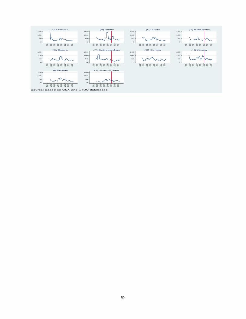
89

0

50

100

150

2001

2003

2005

2007

2009

2011

2013

2015

(A) Adama

0

50

100

150

2001

2003

2005

2007

2009

2011

2013

2015

(B) Ambo

0

50

100

150

2001

2003

2005

2007

2009

2011

2013

2015

(C) Asela

0

50

100

150

2001

2003

2005

2007

2009

2011

2013

2015

(D) Bale Robe

0

50

100

150

2001

2003

2005

2007

2009

2011

2013

2015

(E) Dessie

0

50

100

150

2001

2003

2005

2007

2009

2011

2013

2015

(F) Debreberehan

0

50

100

150

2001

2003

2005

2007

2009

2011

2013

2015

(G) Gonder

0

50

100

150

2001

2003

2005

2007

2009

2011

2013

2015

(H) Jimma

0

50

100

150

2001

2003

2005

2007

2009

2011

2013

2015

(I) Mekele

0

50

100

150

2001

2003

2005

2007

2009

2011

2013

2015

(J) Shashemene


Documents

CEREAL MARKET PERFORMANCE IN ETHIOPIAdocuments.worldbank.org/curated/en/... · CEREAL MARKET PERFORMANCE IN ETHIOPIA: Policy Implications for Improving Investments in Maize and Wheat