Embed Size (px)
Citation preview
University of New England
School of Economics
Local Government Performance Monitoring in NSW: are ‘At Risk’ Councils Really at Risk?
by
David Murray and Brian Dollery
No. 2004-15
Working Paper Series in Economics
ISSN 1442 2980
http://www.une.edu.au/febl/EconStud/wps.htm
Copyright © 2004 by UNE. All rights reserved. Readers may make verbatim copies of this document for non-commercial purposes by any means, provided this copyright notice appears on all such copies. ISBN 1 86389 9103

2
Local Government Performance Monitoring in NSW: are ‘At Risk’ Councils
Really at Risk?
David Murray and Brian Dollery ∗∗
∗∗ David Murray was an Honours student in the School of Economics at the University of New England Brian Dollery is a Professor in the School of Economics and UNE Centre for Local Government at the University of New England. Contact information: School of Economics, University of New England, Armidale, NSW 2351, Australia. Email: [email protected].
3
1. INTRODUCTION
NSW local governments are assessed by the NSW Department of Local
Government (DLG) to either be “at risk” or “not at risk”, with this outcome
dependant on the analysis of a range of key performance indicators derived from
comparative performance tables constructed by the DLG on the basis of
information supplied by individual municipalities. In the formation of monitoring
lists, the DLG undertakes a subjective analysis of these indicators to determine
whether a council should be classified as “at risk” or not. In this paper, an
econometric evaluation of these lists is undertaken in order to determine whether
the indicators employed and the results published by the DLG are sufficiently
robust to withstand analytical scrutiny. Put differently, are municipal councils
deemed to be ‘at risk’ on the basis of the DLG analysis of selected key
performance indicators (KPIs) really ‘at risk’ or have they merely been
erroneously classified as ‘at risk’?
The paper itself is divided into eight main parts. Section 2 provides
relevant institutional information by way of background to the subsequent
analysis. Section 3 discusses the requirements and selection of the chosen
econometric model. Section 4 outlines the methodology of the model. Section 5
appraises the monitoring list for the year 2000/01, whereas Section 6 analyses the
monitoring list for 2001/02. Section 7 examines the monitoring list for 2001/02.

4
Section 8 focuses on the overall robustness of the monitoring lists through the use
of the indicators employed by the DLG. The paper ends in section 9 with some
brief concluding comments on the policy implications of the empirical analysis.
2. INSTITUTIONAL BACKGROUND
As part of its drive to improve the transparency of the public sector, the NSW state
government requires councils to submit annual reports on their performance
covering eighteen areas, including financial results, infrastructure status,
employment information, and progress made in meeting specified external
legislative requirements. The NSW DLG then uses this information to compile
annual comparative performance tables based on various key performance
indicators. The information contained in these comparative performance tables
detail each council’s performance in eleven categories, with a total of thirty
different performance indicators employed. Appendix Table 1 summarises the
resultant KPIs.
The DLG presents data on the state high scores, low scores, means and
medians for each indicator and breaks the results down into the eleven categories
shown in Appendix Table 1. Individual municipalities are grouped into eleven
discrete subsets, ranging from ‘urban capital city’ through to ‘rural remote large’,
in order to facilitate comparisons of structurally similar local authorities by

5
aggregating presumed ‘peer’ councils, despite recognising that ‘when assessing the
performances of councils, it is important to remember that local circumstances can
influence how well a council provides its services’ (DLG, 2004a, p.11).
Following this procedure, the DLG constructs ‘monitoring lists’ of councils
containing those local authorities that have been identified as experiencing the
greatest financial difficulty. These lists have been made public since the financial
year 2000/01 in the DLG’s annual reports. For the three financial years from
2000/01 to 2002/03, a total of 37 councils have appeared on the monitoring lists.
Moreover, 14 councils have appeared thrice; 13 councils have appeared twice, and
10 councils have appeared once. For each successive year, the number of
municipalities listed has grown (from 20 in 2000/01, 29 in 2001/02, to 30 in
2002/03). The KPIs used in compiling these listed are shown in Table 1:
TABLE 1 FINANCIAL PERFORMANCE INDICATORS
Sources of revenue from ordinary activities
Total ordinary activities revenue per capita
Dissection of expenses from ordinary activities
Total expenses from ordinary activities per capita
Current ratio (unrestricted)
Debt service ratio
Capital expenditure ratio Source: Compiled from DLG (2004a)

6
Councils that appear on the published monitoring lists are deemed by the
DLG to be ‘at risk’. They can then be subject to various onerous sanctions, ranging
from closer scrutiny by the DLG to outright dismissal. It is thus obviously
imperative that the procedures involved in determining ‘at risk’ councils be sound
and that municipalities identified to be ‘at risk’ are in fact in serious difficulties.
3. MODEL SELECTION
The selection choice of “at risk” or “not at risk” immediately suggests the use of
econometric models with dependant variables that are dichotomous in nature; this
dependant binary result must arise from an analysis of a range of independent
variables. Linear models utilising ordinary least squares (OLS) methodology fail
to address the “either/or” criterion that is employed, and may in fact provide
probabilities of expected results that fall either side of a bound of 0 and 1. As a
result, non-linear models are more appropriate (Carter Hill, 2001). Non-linear
models will allow the dependant variable to viewed as the probability of
occurrence, which by nature must fall within a 0 and 1 bound (Kennedy, 2003).
A cumulative density approach employing the probit model will provide
for an “S” shaped curve constrained to a 0 and 1 y-axis, where the curve’s slope
will change as the values of the independent variable change. Consequently, the

7
probit function provides the probability of a normal random variable falling to the
left of a particular critical value and can be stated as (Carter Hill, 2001, p.371):
∫∞−
=≤=u
zZPzFπ2
1][)( e-.5u2du
Where: Z is a normal random variable
z is a critical value
The statistical probit model, which expresses the probability that the
dependant variable will take the value of 1, can be expressed as (Carter Hill, 2001,
p.372):
p = P[Z ≤ β1 + β2x] = F[β1 + β2x]
Where: p is the probability
F is the probit function
This model assumes normally distributed errors and utilises maximum
likelihood estimates, where the function provides that the probability of
occurrence is 1, and that the probability of non-occurrence to be 1 minus the
function. Consequently, the likelihood is the resulting product of two elements, the
resultant product of probit functions for all observed occurrences, and the resultant
product of all one minus the probit functions for all observed non-occurrences.
However, in contrast to OLS estimates, the estimated coefficients do not indicate
the effect of marginal changes in the explanatory variables on the probability.

8
Instead they provide for a function of that coefficient. Kennedy (2003) has argued
that an adequate ‘goodness of fit’ for the model would be to sum the fractions of
the correctly predicted number of zeros and the predicted number of ones, with a
‘good’ model exceeding unity.
This paper employs the probit model of estimation, since the two possible
results are either “at risk” or “not at risk”, which are binary in nature, and where
results must fall within these bounds. Secondly, these two possible results are
dependant on a range of indicators that are used by the DLG. Finally, this model
allows us to examine the impact of a change in the value of indicators. Moreover,
since the number of councils in NSW is sufficiently large, it can expected that
maximum likelihood estimators will be normally distributed and consistent (Carter
Hill, 2001).
4. METHODOLOGY
The data used in the compilation of the published comparative tables is available
in an electronic spreadsheet form from the DLG and covers the period from
1994/95 to 2002/03 in individual worksheets (DLG, 2004b). This data incorporates
the 11 categories of KPI as shown in the Appendix Table 1, and it dissects these
KPI’s into their more specific components as shown by the sub-KPI’s in Appendix
9
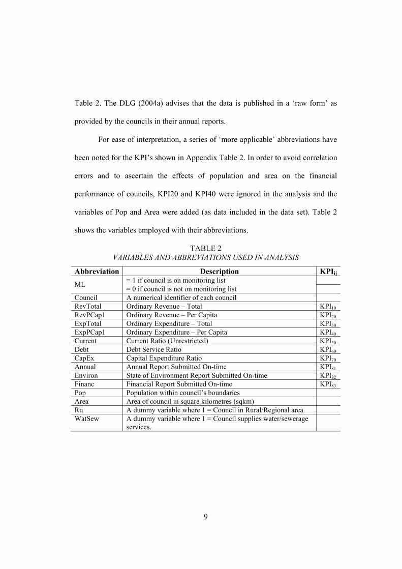
Table 2. The DLG (2004a) advises that the data is published in a ‘raw form’ as
provided by the councils in their annual reports.
For ease of interpretation, a series of ‘more applicable’ abbreviations have
been noted for the KPI’s shown in Appendix Table 2. In order to avoid correlation
errors and to ascertain the effects of population and area on the financial
performance of councils, KPI20 and KPI40 were ignored in the analysis and the
variables of Pop and Area were added (as data included in the data set). Table 2
shows the variables employed with their abbreviations.
TABLE 2 VARIABLES AND ABBREVIATIONS USED IN ANALYSIS
Abbreviation Description KPIij
= 1 if council is on monitoring list ML = 0 if council is not on monitoring list Council A numerical identifier of each council RevTotal Ordinary Revenue – Total KPI10
RevPCap1 Ordinary Revenue – Per Capita KPI20
ExpTotal Ordinary Expenditure – Total KPI30
ExpPCap1 Ordinary Expenditure – Per Capita KPI40
Current Current Ratio (Unrestricted) KPI50
Debt Debt Service Ratio KPI60
CapEx Capital Expenditure Ratio KPI70
Annual Annual Report Submitted On-time KPI81
Environ State of Environment Report Submitted On-time KPI82
Financ Financial Report Submitted On-time KPI83
Pop Population within council’s boundaries Area Area of council in square kilometres (sqkm) Ru A dummy variable where 1 = Council in Rural/Regional area WatSew A dummy variable where 1 = Council supplies water/sewerage
services.
10
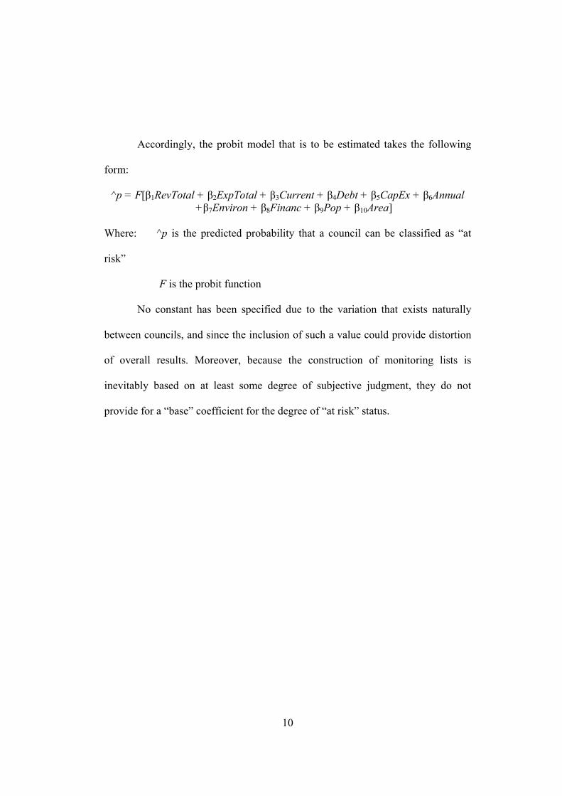
Accordingly, the probit model that is to be estimated takes the following
form:
^p = F[β1RevTotal + β2ExpTotal + β3Current + β4Debt + β5CapEx + β6Annual +β7Environ + β8Financ + β9Pop + β10Area]
Where: ^p is the predicted probability that a council can be classified as “at
risk”
F is the probit function
No constant has been specified due to the variation that exists naturally
between councils, and since the inclusion of such a value could provide distortion
of overall results. Moreover, because the construction of monitoring lists is
inevitably based on at least some degree of subjective judgment, they do not
provide for a “base” coefficient for the degree of “at risk” status.

11
The results obtained have been analysed using a three-stage process:
(i) Is the coefficient sign as per the expectations presented in Table 3.
TABLE 3 EXPECTED SIGNS OF COEFFICIENTS
Variable Expected
Sign Reason
RevTotal – Increased revenue available for service provision, therefore less likely to be “at risk”.
RevPCap1 Not Used ExpTotal + Increased costs of service provision, therefore more likely to
be “at risk”. ExpPCap1 Not Used Current – A higher ratio indicates more assets with fewer liabilities,
accordingly, less likely to be “at risk”. Debt – A lower ratio indicates that debt is a lower proportion of
revenue, therefore the council is less likely to be “at risk”. CapEx – Unity or greater would show that capital equipment is being
replaced in line with depreciation. Annual + Annual report submitted late shows that governance
mechanisms are poor. Environ + State of Environment report submitted late shows that
governance mechanisms are poor. Financ + Financial report submitted late shows that governance
mechanisms are poor. Pop – Larger populations should mean expenditure can be averaged
across a higher number of people. Area + Expenditure should increase in councils with larger areas.
(ii) Each variable is to be tested for significance utilising the following null
hypotheses and alternative hypotheses:
H0: β1 = 0, H1: β1 ≠ 0
H0: β2 = 0, H1: β2 ≠ 0
H0: β3 = 0, H1: β3 ≠ 0
H0: β4 = 0, H1: β4 ≠ 0

12
H0: β5 = 0, H1: β5 ≠ 0
H0: β6 = 0, H1: β6 ≠ 0
H0: β7 = 0, H1: β7 ≠ 0
H0: β8 = 0, H1: β8 ≠ 0
H0: β9 = 0, H1: β9 ≠ 0
H0: β10 = 0, H1: β10 ≠ 0
These hypotheses were tested against standard t-values at both the 5% and
10% significance levels, such that t0.25, n>120 = ±1.96, and t0.05, n>120 = ±1.645.
Where the null hypothesis is rejected, it is concluded that sufficient evidence
exists to claim significance of that variable in the likelihood of being
categorised as “at risk”.
(iii) Using a ratio of the overall proportion of successfully predicted results,
the model will be tested for goodness of fit as discussed earlier. This
will be used in place of traditional R2 values, where a higher ratio will
indicate the degree of accuracy that the model displays. This will allow
judgment to be made upon how “good” the model has been in
predicting econometrically whether a council is “at risk” or not based
upon the observed monitoring list for that year.
13
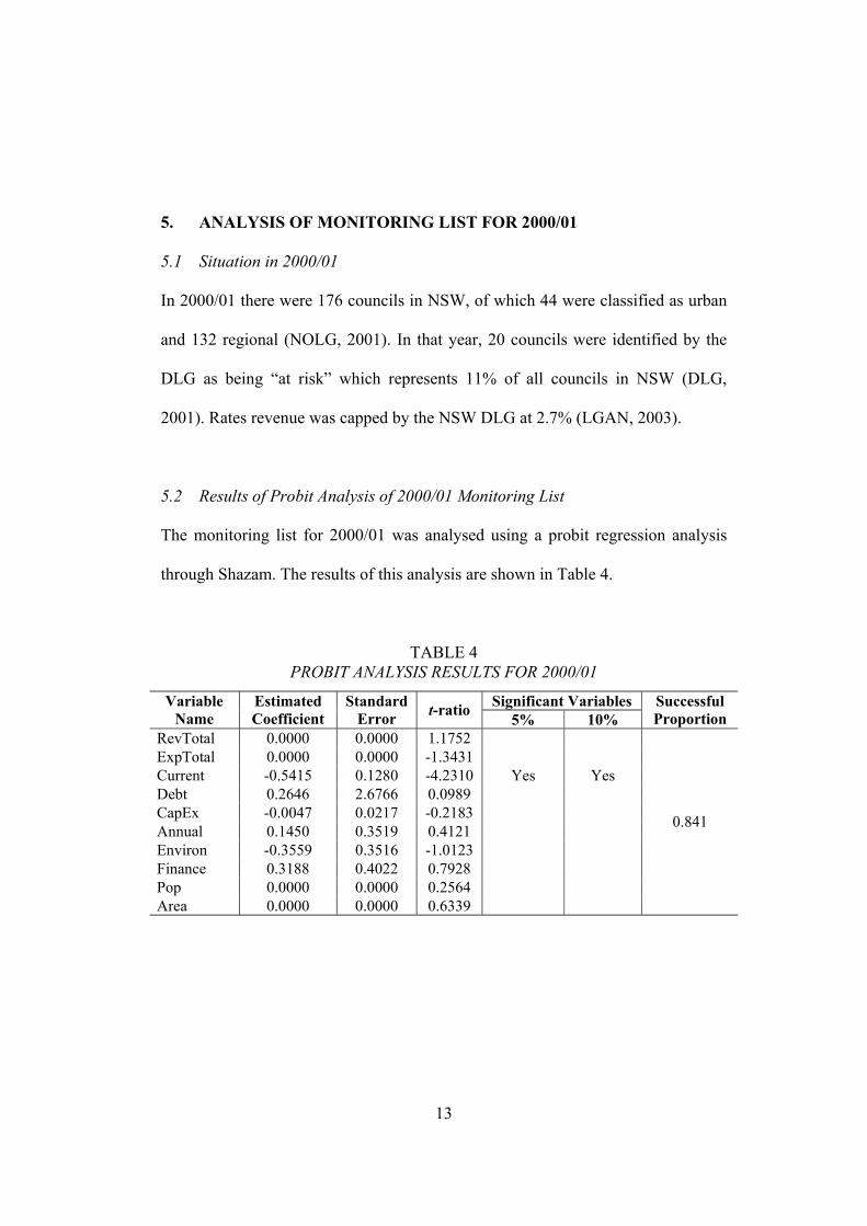
5. ANALYSIS OF MONITORING LIST FOR 2000/01
5.1 Situation in 2000/01
In 2000/01 there were 176 councils in NSW, of which 44 were classified as urban
and 132 regional (NOLG, 2001). In that year, 20 councils were identified by the
DLG as being “at risk” which represents 11% of all councils in NSW (DLG,
2001). Rates revenue was capped by the NSW DLG at 2.7% (LGAN, 2003).
5.2 Results of Probit Analysis of 2000/01 Monitoring List
The monitoring list for 2000/01 was analysed using a probit regression analysis
through Shazam. The results of this analysis are shown in Table 4.
TABLE 4 PROBIT ANALYSIS RESULTS FOR 2000/01
Significant Variables Variable
Name Estimated Coefficient
StandardError t-ratio 5% 10%
Successful Proportion
RevTotal 0.0000 0.0000 1.1752 ExpTotal 0.0000 0.0000 -1.3431 Current -0.5415 0.1280 -4.2310 Yes Yes Debt 0.2646 2.6766 0.0989 CapEx -0.0047 0.0217 -0.2183 Annual 0.1450 0.3519 0.4121 Environ -0.3559 0.3516 -1.0123 Finance 0.3188 0.4022 0.7928 Pop 0.0000 0.0000 0.2564 Area 0.0000 0.0000 0.6339
0.841
14
Table 4 shows that of the ten variables that were chosen, only the current
ratio was significant at both the 5% and the 10% significance level. The estimated
coefficient of zero for total revenue, total expenditure, population, and area is
unexpected and thus does not influence the monitoring list formation. Of the other
variables, unexpected signs were obtained for the debt service ratio, and the
timeliness of the annual and finance reports. Shazam reports the predicted
successful proportion as 0.841, which indicates that the chosen variables in this
model would predict 84.1% of the observed “at risk” councils for 2000/01.
6. ANALYSIS OF MONITORING LIST FOR 2001/02
6.1 Situation in 2001/02
In 2001/02 there were 175 councils in NSW, of which 44 were classified as urban,
with 131 as regional (NOLG, 2002). In that year, 29 councils were identified by
the DLG as being “at risk” which represents 16.5% of all councils in NSW (DLG,
2002). Rates revenue was capped by the NSW DLG at 2.8% (LGAN, 2003).
6.2 Results of Probit Analysis of 2001/02 Monitoring List
The monitoring list for 2001/02 was analysed using a probit regression analysis
through Shazam. The results of this analysis are shown in Table 5.
15
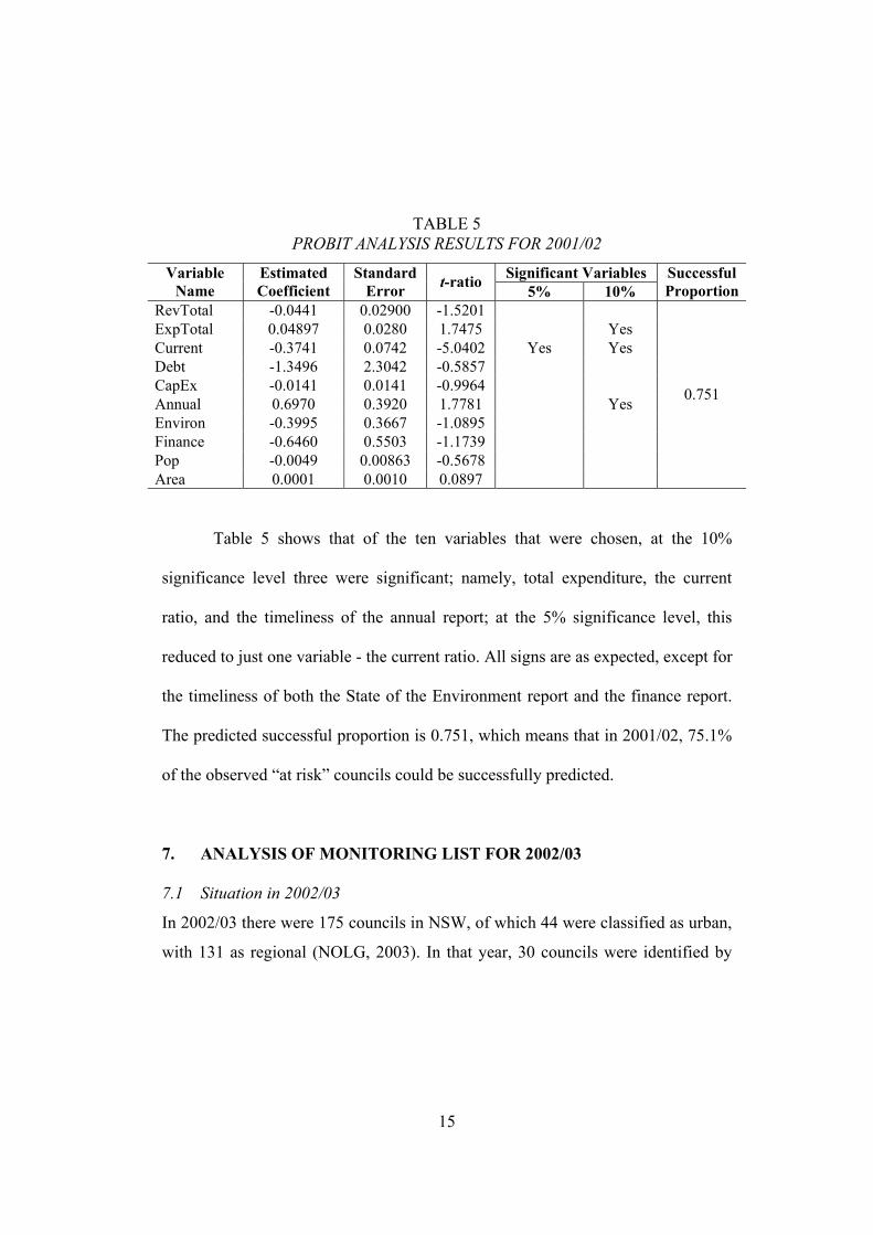
TABLE 5 PROBIT ANALYSIS RESULTS FOR 2001/02
Significant Variables Variable
Name Estimated Coefficient
Standard Error t-ratio 5% 10%
Successful Proportion
RevTotal -0.0441 0.02900 -1.5201 ExpTotal 0.04897 0.0280 1.7475 Yes Current -0.3741 0.0742 -5.0402 Yes Yes Debt -1.3496 2.3042 -0.5857 CapEx -0.0141 0.0141 -0.9964 Annual 0.6970 0.3920 1.7781 Yes Environ -0.3995 0.3667 -1.0895 Finance -0.6460 0.5503 -1.1739 Pop -0.0049 0.00863 -0.5678 Area 0.0001 0.0010 0.0897
0.751
Table 5 shows that of the ten variables that were chosen, at the 10%
significance level three were significant; namely, total expenditure, the current
ratio, and the timeliness of the annual report; at the 5% significance level, this
reduced to just one variable - the current ratio. All signs are as expected, except for
the timeliness of both the State of the Environment report and the finance report.
The predicted successful proportion is 0.751, which means that in 2001/02, 75.1%
of the observed “at risk” councils could be successfully predicted.
7. ANALYSIS OF MONITORING LIST FOR 2002/03
7.1 Situation in 2002/03
In 2002/03 there were 175 councils in NSW, of which 44 were classified as urban,
with 131 as regional (NOLG, 2003). In that year, 30 councils were identified by

16
the DLG as being “at risk” which represents 17.1% of all councils in NSW (DLG,
2003). Rates revenue was capped by the NSW DLG at 3.3% (LGAN, 2003).
7.2 Results of Probit Analysis of 2002/03 Monitoring List
The monitoring list for 2002/03 was analysed using a probit regression analysis
through Shazam. The results of this analysis are shown in Table 6.
TABLE 6 PROBIT ANALYSIS RESULTS FOR 2002/03
Significant Variables Variable
Name Estimated Coefficient
Standard Error t-ratio 5% 10%
Successful Proportion
RevTotal 0.0000 0.0000 -0.0254 ExpTotal 0.0000 0.0000 -0.2684 Current -0.2734 0.0664 -4.1147 Yes Yes Debt 1.2171 1.2981 0.9376 CapEx -0.01391 0.0222 -0.6268 Annual 0.8440 0.4403 1.9171 Yes Environ -0.5572 0.4475 -1.2451 Finance -0.1372 0.3695 -0.3712 Pop 0.0000 0.0000 -0.3007 Area 0.0000 0.0000 0.5378
0.779
Table 6 indicates that of the ten variables that were chosen, at the 10%
significance level two were significant; namely, the current ratio, and the
timeliness of the annual report; at the 5% significance level, this reduced to just
one variable, the current ratio. The estimated coefficient of zero for total revenue,
total expenditure, population and area is unexpected and thus does not influence
the monitoring list formation. Of the other variables, unexpected signs were
obtained for the debt service ratio, and the timeliness of the State of the
Environment report and the finance report. Shazam reports the predicted

17
successful proportion as 0.779, which indicates that the chosen variables in this
model would predict 77.9% of the observed “at risk” councils for 2002/03.
8. DISCUSSION OF RESULTS
Inconsistencies are evident in the results reported in Tables 4, 5 and 6. These
results will be discussed collectively.
8.1 Signs of the Coefficients
Ignoring the significance of the coefficients, there is considerable diversity in the
signs of the coefficients of the ten variables. Expectations were achieved for four
variables in 2000/01, for eight variables in 2001/02, and for three variables in
2002/03. Three variables exhibited signs as per expectations across all monitoring
lists; the current ratio (negative), the capital expenditure ratio (negative), and the
timeliness of the annual report (positive). In 2000/01, the other variable that met
expectations was the timeliness of the finance report (positive). However, this was
not repeated in either of the other years. The other variables that met expectations
occurred in 2001/02 for total revenue (negative), total expenditure (positive), the
debt ratio (negative), population size (negative) and geographic area of the
councils (positive). Of specific interest is that in 2000/01 and 2002/03, total
revenue, total expenditure, population size and geographic area all returned
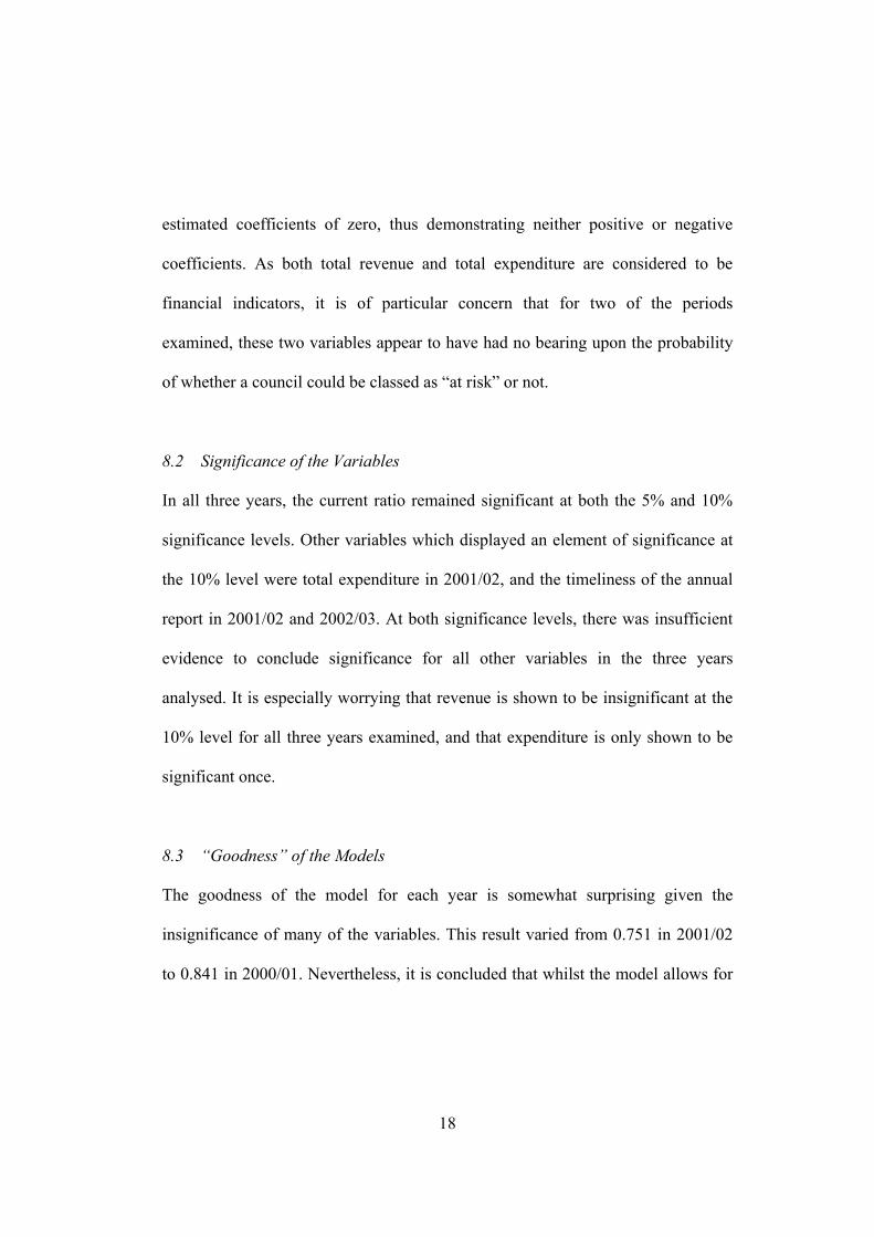
18
estimated coefficients of zero, thus demonstrating neither positive or negative
coefficients. As both total revenue and total expenditure are considered to be
financial indicators, it is of particular concern that for two of the periods
examined, these two variables appear to have had no bearing upon the probability
of whether a council could be classed as “at risk” or not.
8.2 Significance of the Variables
In all three years, the current ratio remained significant at both the 5% and 10%
significance levels. Other variables which displayed an element of significance at
the 10% level were total expenditure in 2001/02, and the timeliness of the annual
report in 2001/02 and 2002/03. At both significance levels, there was insufficient
evidence to conclude significance for all other variables in the three years
analysed. It is especially worrying that revenue is shown to be insignificant at the
10% level for all three years examined, and that expenditure is only shown to be
significant once.
8.3 “Goodness” of the Models
The goodness of the model for each year is somewhat surprising given the
insignificance of many of the variables. This result varied from 0.751 in 2001/02
to 0.841 in 2000/01. Nevertheless, it is concluded that whilst the model allows for
19
prediction of over 75% of observed results (with a high of 84% in 2000/01), there
remains considerable unexplained variation (up to 25%) beyond financial
indicators and report timeliness in the selection of “at risk” councils.
8.4 Robustness of Monitoring Lists since 2000/01
The monitoring lists as published by the DLG are for the specific purpose of
identifying those councils that have “issues of concern with their financial
operations” (DLG, 2003, p.61). In analysing these lists econometrically through
the use of a probit regression model, it has been established that the majority of the
financial indicators employed by the DLG are insignificant at the 10% significance
level, and consequently the analysis performed by the DLG appears to lack a
sound statistical basis. Moreover, whilst consistency in approach might be
expected at least, this is not the case with the changing number of significant
variables, and the discrepancies in sign of the variables over the examined period.
As a result, the determination of financially “at risk” councils in NSW by the
present methods employed by the DLG fails to provide an adequate indication of
financial soundness for those councils which have been placed on monitoring lists
for each year since 2000/01.
20
9. CONCLUDING COMMENTS
This paper has sought to analyse the published monitoring lists of “at risk”
councils in NSW. The results obtained indicate that at present there is no sound
statistical basis for the identification of “at risk” by the NSW DLG.
Three aspects of our econometric results are particularly pertinent. In the
first place, one of the major aims of our analysis has been to determine whether the
methodology that is employed in the identification of “at risk” councils in NSW is
sufficiently robust to withstand analytical scrutiny. It seems that the present
methodology used to analyse councils’ financial data is not valid. For instance, the
probit analysis performed demonstrated that the greater majority of indicators
employed by the DLG in monitoring list construction were insignificant at the
10% level. Moreover, in the goodness of fit analysis, there remained considerable
unexplained variation in the proportion of correctly predicted “at risk” councils
against the actual monitoring lists. Consequently, the conclusion is drawn that the
present methodology employed by the NSW DLG cannot be considered
sufficiently robust to predict actual “at risk” councils.
Secondly, the paper has sought to determine whether the monitoring lists
provided an accurate representation of financial performance of NSW local
authorities to the extent that the financial accountability of councils is adequately
discharged. Our results indicate that the high proportion of insignificant variables

21
raises substantial doubts concerning the ability of the present methodology to
determine “at risk” councils in NSW. It thus cannot be concluded that the existing
monitoring lists provide an accurate representation of “at risk” councils. Moreover,
where financial accountability is sought in the public sector, it is for the specific
purpose that it will call institutions to account for the manner in which they
manage their finances. NSW monitoring lists highlight specific named
municipalities which purportedly display financial inadequacies. However, if the
lists themselves are flawed, then they cannot be considered an adequate tool in
discharging accountability requirements.
Finally, as we have seen, the findings of our paper suggest that those
councils which have been publicly identified as “at risk” may in fact not be in a
parlous financial state at all. This has the potential for opening up a political “can
of worms” for both the NSW Government and the NSW DLG since those councils
which have been labelled as “at risk” could seek legal redress. Moreover, local
authorities which have been branded “at risk” may have been subject to
subsequent close scrutiny, and even dismissal, when their actual financial
soundness is in fact no worse than other councils within the same assigned
classification category.

22
APPENDIX
APPENDIX TABLE 1 NSW LOCAL GOVERNMENT ANNUAL REPORTS – KEY PERFORMANCE
INDICATORS Category Key Performance Indicator
1 Rating 1.1 Average rate per assessment 1.2 Outstanding rates, charges and fees 1.3 Percentage movement in rates and annual charges revenue from previous year 1.4 Percentage movement in user charges and fees from previous year
2 Financial 2.1 Sources of revenue from ordinary activities 2.2 Total ordinary activities revenue per capita 2.3 Dissection of expenses from ordinary activities 2.4 Total expenses from ordinary activities per capita 2.5 Current ratio (unrestricted) 2.6 Debt service ratio 2.7 Capital expenditure ratio
3 Corporate 3.1 Number of equivalent full time staff 3.2 Compliance with statutory reporting deadlines
4 Library Services 4.1 Library expenses per capita 4.2 Circulation per capita
5 Domestic Waste Management and Recycling Services 5.1 Average charge for domestic waste management services per residential
property 5.2 Costs per service for domestic waste collection 5.3 Recyclables – kilograms per capita per annum 5.4 Domestic waste – kilograms per capita per annum
6 Water Supply Services 6.1 Average bill for residential customers ($ per connected residential property) 6.2 Operating costs including depreciation ($ per connected property)
7 Sewerage Services 7.1 Average bill for residential customers ($ per connected residential property) 7.2 Operating costs including depreciation ($ per connected property)
8 Planning and Development Services 8.1 Number of development applications determined 8.2 Mean time in calendar days for determining development applications 8.3 Median time in calendar days for determining development applications 8.4 Legal expenses to total planning and development costs
9 Environmental Management and Health Services
23
9.1 Environmental management and health expenses per capita 10 Recreation and Leisure Services
10.1 Net recreation and leisure expenses per capita 11 Community Services
11.1 Community services expenses per capita Source: Compiled from DLG (2004a)
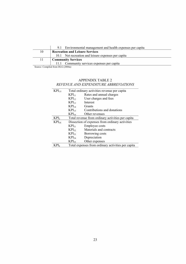
APPENDIX TABLE 2 REVENUE AND EXPENDITURE ABBREVIATIONS
KPI1Y Total ordinary activities revenue per capita KPI11 Rates and annual charges KPI12 User charges and fees KPI13 Interest KPI14 Grants KPI15 Contributions and donations KPI16 Other revenues KPI2 Total revenue from ordinary activities per capita KPI3E Dissection of expenses from ordinary activities KPI31 Employee costs KPI32 Materials and contracts KPI33 Borrowing costs KPI34 Depreciation KPI35 Other expenses KPI4 Total expenses from ordinary activities per capita
24
REFERENCES
Carter Hill, R., Griffiths, W. and Judge, G. (2001).Undergraduate Econometrics, 2nd
Edition, John Wiley and Sons, New York.
Kennedy, P. (2003). A Guide to Econometrics, 5th Edition, Blackwell, Oxford.
Local Government Association of NSW and Shires Association NSW (LGAN) (2003).
Submission No 226 to AHRSC (2003) Rates and Taxes: A Fair Share for
Responsible Local Government, Australian Government Publishing Service,
Canberra.
National Office of Local Government (NOLG) (2001). 2000-01 Annual Report, National
Office of Local Government, Department of Transport and Regional Services,
Canberra.
National Office of Local Government (NOLG) (2002). 2001-02 Annual Report, National
Office of Local Government, Department of Transport and Regional Services,
Canberra.
National Office of Local Government (NOLG) (2003). 2002-03 Annual Report, National
Office of Local Government, Department of Transport and Regional Services,
Canberra.
NSW Department of Local Government (DLG) (2001). 2000-2001 Annual Report, NSW
Department of Local Government, Bankstown.
NSW Department of Local Government (DLG) (2002). 2001-2002 Annual Report, NSW
Department of Local Government, Bankstown.
25
NSW Department of Local Government (DLG) (2003). 2002-2003 Annual Report, NSW
Department of Local Government, Nowra.
NSW Department of Local Government (DLG) (2004a). 2002-2003 Comparative
Information on New South Wales Local Governments, NSW Department of Local
Government, Nowra.
NSW Department of Local Government (DLG) (2004). Comparative Information on
NSW Local Government Councils – Time Series of Comparative Information,
(accessed 5 July 2004) URL: http://www.dlg.nsw.gov.au/dlg/dlghome/dlg_comptime.asp.