Business Cycles and Endogenous Uncertainty�

Rüdiger Bachmanny

RWTH Aachen U. and NBERGiuseppe Moscariniz

Yale U. and NBER

December 2012

Abstract

Recessions are times of increased uncertainty and volatility at both macro and microlevels. This robust empirical pattern is typically interpreted as the result of �uncertaintyshocks�which, propagated through various frictions, impact negatively on aggregate eco-nomic activity. We explore the hypothesis that the causation runs the opposite way:negative �rst moment shocks induce risky behavior, which in turn raises observed cross-sectional dispersion and time series volatility of individual economic outcomes. We focuson consumer price changes. We introduce imperfect information about demand in anotherwise standard monopolistically competitive model. Each �rm is not sure about theelasticity of the demand it faces, but learns it gradually from its volume of sales. In-formation is valuable to choose the optimal mark-up and also, due to a �xed operationcost, potentially to decide whether to exit the market. Preference shocks for each productimpair learning. This demand system is fully microfounded and the model aggregatesto general equilibrium. When deviating from competitors�average prices, a �rm su¤ersa potential pro�t loss, but observes the response of its revenues, thus gains informationabout its market power. Bad economic times are the best times to price-experiment, asthe opportunity cost of price mistakes is lower and exit from the market looms larger.The model is qualitatively consistent with the observed declining hazard rate of CPI pricechanges. Menu costs create a tension between price stickiness and increasing hazard ofprice adjustment. We also present new empirical evidence from CPI microdata support-ing a key prediction of the model: unusually high price volatility signi�cantly raises thechance of exit of the item from the market, even controlling for recessions.

�We thank Veronica Guerrieri and Luigi Paciello for very helpful discussions, David Berger, Je¤ Campbell,Eduardo Engel, Mikhail Golosov, Robert Shimer, Joseph Vavra and audiences at the Kiel Institute-PhiladelphiaFED Dec 2010 conference, Yale macro lunch, and seminars at Collegio Carlo Alberto, Chicago, Atlanta FED,Columbia, 2011 SED annual meeting in Ghent, 2011 NBER Summer Institute, 2012 AEA meetings, 2012Workshop on Macroeconomic Dynamics at the Bank of Italy for comments. We are especially grateful to DavidBerger and Joseph Vavra for coding and performing the empirical work on restricted access CPI microdata atthe BLS. The usual disclaimer applies.

yTemplergraben 64, 52062 Aachen, Germany. E-mail: ruediger-bachmann@gmx.de Web:http://www.vwlmac.rwth-aachen.de/wbaker/wb/pages/team/prof.-ruediger-bachmann-phd.php

zPO Box 208268, New Haven, CT 06520-8268, USA. E-mail: giuseppe.moscarini@.yale.edu Web:http://www.econ.yale.edu/faculty1/moscarini.htm

1

1 Introduction

Bad economic times are also times of rising uncertainty. This refrain �nds substantial empirical

support, and resonated again throughout the Great Recession. In an in�uential paper, Bloom

(2009) o¤ers new evidence and interprets the causality as running from uncertainty to aggregate

economic activity. This view applies not only to uncertainty about the economy�s prospects or

about macroeconomic policy, as re�ected in the time-varying price of risk, but also to micro-

level uncertainty about the fate of individual businesses. Exogenous changes in the volatility

of idiosyncratic shocks, mediated by frictions, impact mean economic activity, and may cause

recessions. In Bloom�s case, the frictions are irreversibility in investment and hiring/�ring, so

increased uncertainty raises the real option value of waiting.

In this paper, we entertain the hypothesis of reverse causality. We explore a mechanism

through which a decline in aggregate economic activity, a �rst moment shock, induces agents

to undertake riskier activities, that result in more dispersed and volatile individual outcomes.

Our view is that negative �rst-moment shocks to a �rm�s pro�tability, whether idiosyncratic or

aggregate, lead the �rm to review its modus operandi and to change its strategy to survive. If

our view is correct, then the root cause of aggregate �uctuations are �rst moment shocks, and

rising uncertainty is an ampli�cation device.

We explore this hypothesis in the context of price-setting. We focus on �rms, because most

of the available empirical evidence on countercyclical dispersion refers to �rm-level measures

of performance. We focus on prices, because this is the margin that �rms can activate most

quickly in response to �rst moment shocks, more so than production inputs, projects/business

ventures, relationships with suppliers and customers.1 Berger and Vavra (2010) document that,

in the micro-data underlying the Consumer Price Index, the dispersion in log price changes is

strongly countercyclical.

We revisit the standard model of monopolistic competition, and further assume that the

�rm does not know exactly the price elasticity of the demand it faces.2 Sales do not fully

reveal market power, because of unobserved preference shocks that a¤ect the distribution of

demand. Due to consumers� preference for variety, the more the price quoted by the �rm

deviates from those quoted by competitors, the more sales re�ect the true elasticity of demand,

1From a leading Marketing textbook (Kotler 2000, p. 456): �Price is the marketing-mix element thatproduces revenue; the others produce costs. Price is also one of the most �exible elements: It can be changedquickly, unlike product features and channel commitments.�

2�Many companies try to set a price that will maximize current pro�ts. They estimate the demand andcosts associated with alternative prices and choose the price that produces maximum current pro�t �ow, cash�ow, or rate of return on investment. This strategy assumes that the �rm has knowledge of its demand andcost functions; in reality, these are di¢ cult to estimate.�(Kotler (2000), p. 462).

1

hence the more informative they are. In good times, �rms choose similar prices, as the scale

of demand is high and pricing deviations, albeit informative, are costly in terms of lost �ow

pro�ts. When a �rm observes a string of poor sales, it becomes increasingly pessimistic about

its own market power, and starts contemplating the exit decision. At that point, the returns

to price experimentation, changing prices in order to learn the demand curve, increase. The

�rm makes a (possibly last) attempt to understand whether its product sells well or should

be discontinued. When a negative aggregate pro�tability shock hits the economy, the cost of

experimenting and learning for the good times falls, because business is slow anyway, and the

returns rise, as exit looms larger and �rms �gamble for resurrection�. As �rms try harder to

learn their demand curves, they modify their prices drastically, generate more variable and

informative sales, and further adjust prices in response to what they observe. So the dispersion

and volatility of price changes rise. On the other hand, when exit becomes very likely, the �rm

puts less weight on continuation, when information will be useful, a reason to experiment less.

To assess all these e¤ects we explore numerical examples. First, we present results in par-

tial stochastic equilibrium, and verify that the dispersion of price changes indeed comoves in-

versely with aggregate economic activity. Second, we calculate steady state general equilibrium,

when aggregate productivity is constant and optimal prices quoted are consistent with market

clearing. The comparative statics e¤ects across steady states of changes in aggregate labor

productivity on price dynamics are parallel those of aggregate shocks in partial equilibrium.

This exercise reveals that a burst in price volatility is more often followed by exit. We test

this prediction with CPI microdata from the BLS. We �nd that, controlling for the average price

volatility of a CPI item, for the CPI in�ation rate and average frequency of price adjustment

in the sector to which the item belongs, and for the state of the business cycle, high volatility

of an item�s price in the previous four months has a very strong and highly signi�cant positive

e¤ect on the chance that the same item is taken o¤ the market by its producer/seller.

As mentioned, the real option literature suggests that increased uncertainty discourages and

delays irreversible actions, such as investing in new capital, hiring new workers, or changing

prices in the presence of non convex adjustment costs. This prediction is not a foregone outcome.

Larger shocks increase inertia by inducing �rms to move their optimal adjustment boundaries

further apart, to take advantage of the larger option value of waiting, but also push �rms

faster against adjustment boundaries, so the net e¤ect is ambiguous. Bloom (2009) in partial

equilibrium, and Bloom, Floetotto and Jaimovich (2009) in general equilibrium, investigate

this mechanism, allowing for �xed and variable adjustment costs to labor and capital. A

calibrated S,s investment model, with garden variety aggregate shocks in mean productivity

and less traditional innovations in the volatility of �rm-speci�c shocks, shows that the latter

2

can independently cause a drop in aggregate investment and hiring, and even a recession of

plausible magnitude, followed by a sharp rebound as uncertainty is resolved.

Empirical measures of micro-level volatility tend to lag the cycle, and rise in nearly all re-

cessions for which data are available. Aggregate asset price volatility does not lag, but is not

always followed by a recession, as after the stock market crash of 1987 and the Asian crisis

of 1997. This is suggestive of a causal e¤ect from recessions to micro-level uncertainty, with

a relatively quick response of the latter to the former. Our goal here is not to diminish the

importance of uncertainty shocks, but rather to explore the viability of alternative explanations

for countercyclical uncertainty. The mechanism stressed by Bloom (2009) may still operate:

faced with �xed input adjustment costs, �rms that willingly undertake risky actions on other

margins, such as pricing or marketing, anticipate receiving news, good or bad, so they have an

incentive to wait for those news before investing or hiring. The direction of causality, however,

matters for economic policy. If agents are creating idiosyncratic risk, macro stabilization pol-

icy will also reduce micro-level uncertainty, a not necessarily desirable by-product, because it

impairs learning and interferes with e¢ cient resource reallocation.

Besides business cycles, imperfect information about the price sensitivity of demand gen-

erates two new predictions for price-setting. First, price experimentation imparts an upward

bias in prices. A �rm can learn by deviating from competitors�prices both up and down, and

then observing the impact on sales, but a high price has the additional bene�t of reducing

physical sales, thus production costs. This seems a more general principle, which goes beyond

the isoelastic utility framework. Since experimentation is more valuable when the �rm is at

risk of bankruptcy, that is in recessions, the upward bias is countercyclical.

The second prediction pertains to the dynamics of individual prices: the volatility of price

changes declines over time. A price change away from competitors�reveals information about

the demand curve. Therefore, larger subsequent changes are more likely, as more information

accrues. Volatility begets volatility. As the truth is revealed, the price settles. In terms of

testable predictions, large price changes away from competitors�prices should be likely followed

soon by more large price changes, and the probability of a non-negligible price change declines

with its duration. Our model provides a natural explanation for a hazard rate of price changes

decreasing with price duration. When a �rm adjusts a price, it learns much new information,

which may cause a new adjustment. These two phenomena are exactly what Campbell and

Eden (2010) �nd in weekly scanner data for groceries from two US cities, after controlling for

temporary sales. They conclude: �Taken together, these results suggest to us that sellers exten-

sively experiment with their prices.�3 In contrast, time- and state-dependent price adjustment

3Nakamura and Steinsson (2008) also �nd a decreasing hazard rate of price changes in CPI items, except for

3

models imply a constant or increasing hazard rate. Indeed, we explore a steady state equi-

librium of our model where �rms face also menu costs to adjust prices. The optimal inaction

region is two-dimensional, in the space of price imbalance and beliefs about the demand curve.

Menu costs tilt the hazard rate of price adjustment up again, in contrast with the empirical

evidence.

Our modeling contribution is the introduction of demand-curve uncertainty in the stan-

dard equilibrium model of monopolistic competition. Crucially, prices impact revenues via the

true price elasticity, while the confounding shocks to the level of demand are independent of

prices quoted, so the �rm can control the �ow of information by manipulating the price. This

has a cost, forgone static pro�ts, which is larger the more the �rm deviates from the aver-

age price quoted by competitors. The strategic complementarity of prices implies strategic

substitutability in information acquisition. In contrast to the literature which provides infor-

mational microfoundations to price adjustment costs (e.g., Alvarez, Lippi and Paciello 2011),

in our setting the tool to acquire information is the price itself, and the cost of information

acquisition is endogenous. One implication is that the hazard rate of price adjustment tends

to decline in duration. The multi-armed bandit literature on the �ignorant monopolist�, that

learns its own demand function through pricing decisions, o¤ers several tractable but rather ad

hoc models, which posit a primitive, ad hoc noisy demand function. See Tre�er (1993) for an

example. To the best of our knowledge, ours is the �rst general equilibrium model of Bayesian

experimentation. It is fully microfounded, preserves nice aggregation properties, and can be

solved numerically. The �rm�s equilibrium �ltering problem can easily be extended in several

directions, for example �quality obsolescence�: the introduction of new products stochastically

increases the price elasticity of demand of pre-existing products, in a way that the �rm cannot

directly observe and can learn only from declining sales.

The paper is organized as follows. Section 2 reviews existing research on uncertainty at

cyclical frequencies, to motivate our exercise and to place it in the proper context. Section 3

describes the economy, Section 4 the problem of the household, which generates the demand

curve faced by �rms under imperfect information, Section 5 the �rm�s optimal �ltering and

pricing experimentation problem, Section 6 de�nes general equilibrium. Section 7 illustrates

numerically the individual �rm problem in a stochastic economy and steady state general equi-

librium. Section 8 introduces menu costs. Section 9 presents the empirical test of the model�s

predictions with CPI microdata. Section 10 concludes with a description of feasible extensions

of the model.

annual spikes in some services that are re-priced every 12 months. Vavra (2010) controls for unobserved itemheterogeneity and �nds that the hazard rate strongly declines in the �rst two months since last adjustment. SeeAlvarez, Lippi and Paciello (2011) for an extensive discussion of hazard rates.

4

2 Uncertainty and the business cycle

It has long been known that �nancial markets are more volatile when asset prices su¤er, typically

in bad economic times. Campbell et al. (2001) document that the volatility of individual

stock prices negatively comoves with detrended GDP. Bloom (2009) shows that the VXO index

of stock market volatility covaries negatively with industrial production, and positively with

cross-sectional dispersion in pro�ts and stock returns. As mentioned, the scholarly narrative

interprets changes in uncertainty as random changes in the standard deviation of idiosyncratic

shocks, which impact aggregate economic activity. Indeed, Bloom (2009) �nds that positive

innovations to the VXO index in a VAR identi�ed by Choleski-ordering cause a sharp drop and

rebound in industrial production.

More recently, the attention has moved to uncertainty in macroeconomic policies, and un-

certainty thereof. Baker et. al (2012) measure uncertainty in macroeconomic policy from news

media. Born and Pfeifer (2012), and Fernandez-Villaverde et al. (2011, 2012) estimate un-

certainty in fundamentals, monetary and �scal policy, and show that shocks to uncertainty

about future policy have a discernible but small impact on real activity and in�ation in an

otherwise standard New Keynesian model. General equilibrium e¤ects, notably the drop in the

interest rate, erase most of the e¤ects identi�ed by Bloom (2009) in partial equilibrium. Basu

and Bundick (2012) and Johanssen (2012) show that shocks to the volatility of (resp.) funda-

mentals, such as discount factors and technology, and of �scal policy have a sizable impact on

real activity if and only if the economy is close to the Zero Lower Bound, because the general

equilibrium e¤ect is muted. The last �ndings require, of course, strong nominal rigidity, and

appear fragile in light of Vavra (2012)�s result that nominal rigidity and money non-neutrality

are severely reduced in recessions, because the distribution of price changes also experiences a

large increase in spread (Berger and Vavra 2010), so �rms change prices more independently of

monetary shocks.

We are interested, instead, in cyclical movements in cross-sectional measures of dispersion in

outcomes, primarily across �rms. Aggregate volatility comoves with micro-level �uncertainty�.

Bloom et al. (2012) document that the dispersion of shipments across manufacturing estab-

lishments, of growth rates of sales across listed companies and across all industries are strongly

countercyclical The precise mechanism through which uncertainty shocks cause recessions relies

on the type of friction that impedes continuos microeconomic adjustment.4

4An early version of this idea is Lilien (1982)�s sectorial reallocation hypothesis, based on frictions in thereallocation of employment across sectors. An increased dispersion in the size of sector-speci�c shocks causestemporary unemployment, as workers slowly retrain and reallocate to expanding industries. Brainard andCutler (1993) measure sectorial shocks by means of excess returns on industry stock indices, after controllingfor industry-speci�c betas, and indeed �nd evidence that the dispersion of excess returns moves over time and

5

Bachmann and Bayer (2011a, 2011b) use a long panel of German �rms and show that

the dispersion in �rm-level innovations in TFP, sales and real value added is countercyclical,

although the dispersion in investment rates is procyclical. Unlike much of the previous lit-

erature, they rely on direct measures of performance for a large sample of companies of all

types, not just publicly traded, but also private, and not only in manufacturing, but spanning

all sectors. This direct evidence indeed points to more news in �rms� fundamentals during

recessions. Using this evidence to calibrate a neoclassical economy with non convex adjustment

costs, Bachmann and Bayer conclude that shocks to the variance of �rm-level TFP innovations,

if any, mildly amplify �rst-moment aggregate shocks, but are not an independent source of

aggregate �uctuations. Bachmann, Elstner and Sims (2010) compare measures of individual

business expectations, from surveys of decision makers inside the �rms, with ex post business

performance, to extract a measure of genuine uncertainty. They replace stock market volatility

with mean square error in business forecasts and repeat Bloom (2009)�s VAR exercise. They

�nd a negative, but very persistent, e¤ect of uncertainty shocks on industrial output. The real

option approach predicts a sharp but short-lived e¤ect. Next, as an alternative (to ordering)

identi�cation strategy, they require that structural uncertainty shocks have no long-run e¤ects

on aggregate economic activity. They �nd that these shocks have no discernible impact even

in the short run. Conversely, various measures of uncertainty signi�cantly increase in response

to an identi�ed long-run negative shock to aggregate economic activity.

Gilchrist, Yankov and Zakrajsek (2009) reach a similar conclusion from asset prices. They

construct commercial credit spreads from a large panel of US non�nancial �rms, isolate the

component that is orthogonal to those �rms�stock prices and to contemporaneous macroeco-

nomic conditions, and show that this component explains in a VAR framework a signi�cant

fraction of the variability of aggregate employment, but at medium horizons. A natural source

of credit spread shocks are uncertainty shocks mediated by agency frictions in �nancial mar-

kets. Arellano, Bai and Kehoe (2011) and Di Tella (2012) argue that positive shocks to both

idiosyncratic and aggregate uncertainty generate, through borrowing constraints, recessions of

plausible magnitude.

Finally, a few authors have followed our early lead and entertained the hypothesis that

changes in cross-sectional dispersion may be the result, and not the cause, of business cycles.

Cui (2012) explains increasing dispersion in �rm-level TFP in recessions through the combina-

tion of credit frictions, which prevent �rms in good shape from buying assets, with the desire

of distressed �rms to develerage and unload costly debt before selling their assets and used

strongly correlates with unemployment. Its explanatory power for unemployment, however, is quantitativelyweak. Davis, Haltiwanger and Schuh (1996, Figure 5.5) �nd that the dispersion of employment growth ratesacross manufacturing establishments is signi�cantly larger in 1982 (recession) than in 1978 (expansion).

6

capital. The slowdown in used capital reallocation, indeed observed in recessions, expands

TFP dispersion. Closer to our work is the hypothesis in D�Erasmo and Moscoso-Boedo (2012).

When a negative aggregate TFP shocks hits, �rms �nd it optimal to scale down intangible in-

vestment in market access, such as marketing, advertising, brand development, or organization

development. This drop in market investment reduces the spectrum and size of the markets

that the �rm can access, which provides less averaging and exposes the �rm to more risk. The

motivation is their empirical �nding in a �rm-level dataset that �rm-level volatility in sales

is countercyclical while intangible investment is procyclical, and more generally idiosyncratic

volatility and intangible investment are negatively correlated across �rms. As in our work, they

emphasize demand shocks at the �rm level and �rst-moment aggregate shocks. In our model,

the �investment�in market access is price experimentation itself.

3 The economy

Time is discrete. There exist a continuum of di¤erentiated varieties of a perishable consumption

good or service, indexed by (j; k), j 2 (J1 [ J2), k 2 [0; 1]. Each variety is produced by a single�rm using only labor: h units of labor time produce z

�h� �h

�physical units, where �h � 0 is

minimum employment required to keep the �rm in operation, and z is aggregate productivity,

which follows a Markov process.

Firms are owned by fully diversi�ed, identical individuals, whose preferences for consumption

C and work time H are expressed by the utility function

logC � �H1+�

1 + �

where

C =pC1C2

is a composite consumption good, and for i = 1; 2

Ci =

�ZJi

Z 1

0

�1�ik c

�i�1�ij;k dkdj

� �i�i�1

(1)

is a CES aggregator of quantities cj;k � 0 consumed of varieties (j; k) 2 Ji� [0; 1]. Here �k � 0are preference weights. Of the two indices (j; k) that identify a variety, j is time-invariant,

while k, which determines the weight �k, is drawn every period independently over time and

of j from a uniform distribution on [0; 1]. The draw k is the same for all consumers. Thus,

the weight �k acts as variety-speci�c preference shock. We identify varieties with a bi-variate

7

index j; k in order to allow for preference shocks (k) independent of the identity and price of

the variety (j).

There are two types, or baskets, of varieties: �specialties�j 2 J1, hard to substitute for eachother, with elasticity of substitution across varieties �1 > 1, and �generics� j 2 J2, mutuallysubstitutable, with higher elasticity of substitution �2 > �1. We denote by i the measure of

type i varieties, the Lebesgue measure of set Ji. Finally, � > 0 is the inverse Frisch elasticity

of labor supply and � > 0 the relative disutility of labor.

Each consumer supplies laborH on a competitive market at wage rate w, and receives pro�ts

� from the �rms she owns. She chooses every period consumption of all varieties j; k, sold at

prices Pj;k, and labor supply, to maximize utility subject to her budget constraint. This is a

static problem solved anew each period, because consumers have no access to capital markets

in this economy.

Each period, each �rm (j; k) posts a price Pj;k for its variety and hires labor to produce

and serve all demand at that price. The �rm�s objective is to maximize the expected present

value of �ow pro�ts, net of labor costs, including the �xed �operation�cost = w�h per period,

discounted with factor � 2 (0; 1).5 The discount factor incorporates both time preferences ofthe households, who own the �rms, and a (constant) chance of exogenous exit of the �rm due

to some idiosyncratic destruction shock. When the �rm (variety) exits, its continuation value

is normalized to zero.

The novel element in our model is the information structure. Each period, the representative

consumer knows her preferences, so the draws of all k0s within each basket i, before supplying

labor and making purchases; so, she knows how easily substitutable in her own preferences

each variety j is. Conversely, the �rm does not observe its own identity (j; k), thus whether

it is a high- or low-market power �rm (is j 2 J1 or 2 J2?) and the preference weight �k thatthe consumer puts on its variety. For example, the consumption good is fruit, the units of all

varieties are pounds of fruit, �rm j produces kiwis, but does not know whether consumers see

kiwis as similar to such staples as apples and oranges, di¢ cult to substitute, or as another kind

of berries, which are more price sensitive. And the consumer likes some type of kiwis (j; k)

better than others (j; k0), randomly every period.

When a �rm enters the industry, Nature draws the basket i to which the variety produced

by the entering �rm belongs to be i = 1 with chance �0, which is also the �rm�s prior belief that

it is of type 1. The price quoted a¤ects sales through the elasticity of demand, but preference

shocks create demand level shocks, which hide the true elasticity. Over time, the �rm observes

5We are implicitly assuming that �rms, unlike households, have access to a perfect capital markets, so thatonly the expected present value, and not the timing, of pro�ts matters. A �rm can operate as long as theexpected continuation value more than compensates for any current loss.

8

the prices it quotes and the resulting volumes of sales, and learns from them the price elasticity

of the demand it faces.

We choose to make the elasticity �i and not the scale � of the demand curve the persistent,

unobserved component that �rms are interested in estimating. The reason is that, in the CES

preference setup, the scale of demand does not a¤ect the optimal price, and experimentation

is �passive�. In contrast, when demand elasticity is unknown, the �rm can trace the demand

curve, up to noise, by changing the price. Thus, the �rm faces an interesting trade-o¤ between

current pro�ts and information about the optimal markup to charge in the long run.

4 Consumer optimization

The complete description of the consumer-worker problem is:

maxH;fcj;kg

(j;k)2A

1

2

2Xi=1

�i�i � 1

log

�ZJi

Z 1

0

�1�ik c

�i�1�ij;k dkdj

�� �H

1+�

1 + �

s.t.2Xi=1

ZJi

Z 1

0

Pj;kcj;kdjdk = Y

Y = wH +�

The consumer chooses labor supply H and earns total income Y , then she decides how much

income to spend on each basket and how to allocate that amount within each basket across

varieties.

First, we solve the �outer� problem of choosing labor and allocating spending between

baskets. For ease of presentation, we guess that there exist price indices �Pi so that we can write

the budget constraint as�P1C1 + �P2C2 = wH +�

We will later verify this guess and solve for �Pi. The problem becomes

maxCi;H

logpC1C2 � �

H1+�

1 + �+ �

�wH +�� �P1C1 � �P2C2

�Taking FOCs for Ci

�P1C1 = �P2C2 =1

2�:

Using the budget constraint, due to the Cobb-Douglas nature of the �outer�preference aggre-

gator, the consumer spends Y=2 on each basket, independently of prices:

�P1C1 = �P2C2 =Y

2=wH +�

2

9

Taking a FOC for labor supply and using the above equations to solve out for the multiplier �,

�H� = �w =w

Y=

w

wH +�(2)

we obtain an equation solved implicitly by labor supply Hs (w;�).

Next, the consumer optimally allocates her Y=2 budget among varieties (j; k) within basket

i. The FOC for an optimal cj;k is

1

2

�1�ik c

� 1�i

j;kRJi

R 10�

1�ik c

�i�1�ij;k djdk

= �Pj;k

So the consumer equates the ratio �1�ik c

� 1�i

j;k =Pj;k between any two j; k and j0; k0 in the same

basket, and

cj0;k0 = cj;k�k0

�k

�Pj;kPj0;k0

��iMultiplying this equation through by Pj0;k0 and integrating over j0; k0 2 Ji keeping j; k �xed

Y

2=

ZJi

Z 1

0

cj0;k0Pj0;k0dj0dk0 =

cj;k

�kP��ij;k

ZJi

Z 1

0

�k0P1��ij0;k0 dj

0dk0

we obtain the demand for variety j; k as a function of prices and the total budget Y

cj;kjj2Ji = �kP��ij;k

�P 1��ii

Y

2(3)

where we de�ne the price index:

�P 1��ii =

Z 1

0

�k0

�ZJi

P 1��ij0;k0 dj0�dk0: (4)

Using this expression into the demand (3) for each variety, and the resulting expression into (1)

for the basket Ci, and using (4) for �Pi again, after some algebra we verify the guess �PiCi = Y=2:

We invoke a Law of Large Numbers for distribution (Glivenko-Cantelli theorem) and inde-

pendence of the draws of k from j to conclude that the price index �Pi is independent of the

actual realization of the k draws, and every �rm knows each �Pi. Intuitively, the demand shocks

�k average out, because there are a continuum of them for each variety of type j, although the

�rm does not observe the speci�c realizations of the demand shocks. There is no correlation

between demand shock �k0 and price quoted Pj0;k0, because the �rm quotes the price before the

demand shock is realized (in a i.i.d. fashion), and anyway the �rm does not observe the demand

10

shock even ex post; it only observed realized sales. So Pj0;k0 is independent of k0:Without loss

in generality, we can normalize the scale of demand shocks so thatR 10�k0dk

0 = 1, so that

�P 1��ii =

ZJi

P 1��ij0;k0 dj0dk0:

Note that if the measure i of active �rms of type i, the Lebesgue measure of set Ji, increases,

given individual prices, the rescaled price index �P 1��ii increases, because it is a sum of inverse

prices, not a mean. Then, the demand cj;kjj2Ji for each variety of type i falls, due to more

intense competition for the budget spent on basket Ji when this includes more varieties, a

standard preference for variety e¤ect. In contrast, the demand for varieties of the other type is

una¤ected, because the shopper always splits her budget equally between the two baskets.

5 Firm optimization

5.1 Bayesian updating

A �rm enters the industry with a prior belief �0 that its variety has low demand elasticity �1(high mark-up). Each period the �rm quotes a price Pj;k and observes the quantity Qj;k it sells.

But the �rm knows neither the customer�s preference shock (�k) nor its own demand elasticity

(�i). Taking logs in the demand function (3), a �rm j; k that is really of type i and receives

preference shock �k (but does not know either i or k) observes physical sales of

qj;k = ��ipj;k + y + �i + "k (5)

where

qj;k = logQj;k, pj;k = logPj;k, y = log Y , "k = log�k, �pi = log �Pi, �i = (�i � 1) �pi � log 2

Here the demand shock "k hides from the �rm its true price elasticity �i. The term �i sum-

marizes aggregate variables that also determine demand, namely the log price �pi index quoted

by the relevant (same type i) competitors, which depends on the measure of varieties that

consumers buy. Therefore, given a log-price quoted pj;k, demand can be high for one of three

reasons: the variety is hard to replace in consumer preferences (j 2 J1), the consumer placesa large weight on the variety in her preferences this period (high "k), and/or the variety has

few competitors, so �pi (which is an inverse log price index) is high and the consumer spends on

(j; k) much of her total budget Y=2 for the basket.

Without loss in generality, we choose a c.d.f. F and assume that preference shocks are

�k = eF�1(k)

11

Recall that k � U [0; 1], so F is the c.d.f. of the log-demand shock "k

Pr ("k � ") = Pr (log�k � ") = Pr�F�1 (k) � "

�= Pr (k � F (")) = F (") :

The only restriction on the support of F is the normalizationR 10�kdk = 1:

From now on we drop the variety index j,k in (5) for convenience, so y; p; q are public

information, while i and " are only observed by the consumer. A �rm that currently believes

to be of type 1 with probability �, quotes price p and observes sales q and aggregate income y,

all in logs, updates by Bayes rule its belief to:

�0 = B (�; p; q; Y ) =

�1 +

1� ��

F 0 (q � �2 + �2p� y)F 0 (q � �1 + �1p� y)

��1(6)

where F (~q � �i + �ip� y) = Pr (q � ~qji). The distribution of demand shocks F does not

depend on aggregate income Y = ey, to avoid introducing an exogenous source of cyclical

uncertainty, which is the whole point of our analysis.

Dynamic decision-making requires knowing the evolution of beliefs conditional on a given

state i, where true sales are q = �i � �ip + y + ". After some algebra, the conditional (ontrue state i) evolution of beliefs is independent of aggregate income Y and we can write it as a

function of prior beliefs, price quoted, and demand shocks as follows

bi (�; p; ") = B (�; �i � �ip+ y + "; q; Y ) =�1 +

1� ��

F 0 (�i � �2 + (�2 � �i) p+ ")F 0 (�i � �1 + (�1 � �i) p+ ")

��1(7)

As usual, the belief bi (�; p; ") that the state is 1 when the true state is i = 1 (2) has a positive

(resp., negative) drift, and unconditionally on the state beliefs are a martingale:

E" [b2 (�; p; ")] < � = �E" [b1 (�; p; ")] + (1� �)E" [b2 (�; p; ")] < E" [b1 (�; p; ")]

The speed of learning, that is how quickly posterior beliefs react to sale volume, is controlled by

the price through its e¤ect on the likelihood ratio, namely the ratio of densities F 0 in (7). For ex-

ample, in state i = 1, that ratio equals F 0 ((�1 � 1) (�p1 � p)� (�2 � 1) (�p2 � p) + ") =F 0 ("). Soa very large deviation of own price from the price index of each basket, jp� �pij, either positive ornegative, provides much information. Alternatively we can write is as F 0

�(�1 � 1) �p1 � (�2 � 1) �p2 + "

��2��1"p+ 1

��=F 0 ("),

so the direct e¤ect of the price on the speed of learning is proportional to the di¤erence in pos-

sible values of elasticities, divided by the scale of the noise, a signal/noise ratio. The higher

this is, the stronger the information �productivity�of price experimentation.

5.2 Optimal pricing

A �rm quotes a price P , that the shopper, fully informed about her own preferences, compares

with the price index �Pi of the immediate substitutes. Revenues are PQ(P ), where Q is the

12

demand function in (3). Costs are wh (variable) and wh = (�xed). Using the production

function and assuming the �rm serves all demand, the total demand for labor equals Q (P ) =z+

h. Putting all together, realized �ow pro�ts for �rm j equal revenues net of variable costs, minus

�xed costs:

� = �Y

2

P��i�P � w

z

��P 1��ii

� = �Y2

�P�Pi

��� �P�Pi� w

z �Pi

��:

To �x ideas, we start with two special cases. First, the �rm knows its demand elasticity. Second,

it learns demand elasticity from sales but is myopic (� = 0). Finally, we move to dynamics

with learning.

5.2.1 Perfect information

If the �rms knows to be in the basket i, hence to face demand elasticity �i, then it also knows

the demand it faces �Y P��i=2 �P 1��i1 up to the possibly unknown and i.i.d. preference shock

�. In this case, the �rm�s problem has no intertemporal dimension and consists of maximizing

�ow pro�ts each period. Using E [�] =R�kdk = 1, the �rm chooses whether to pay the �xed

cost to produce at all and, if so, the price that maximizes expected pro�ts:

max

*0;max

P

Y

2

P��i�P � w

z

��P 1��ii

�+

The optimal price is a constant markup, independent of Y

P PIi=

�i�i � 1

w

z

and the �rm earns maximized expected pro�ts

�PIi= max

*0;Y

2(�i)

��i�

w�Pi (�i � 1) z

�1��i�:

+

Since �1 < �2, type 1 �rms have more market power.

5.2.2 Imperfect information: static optimization

Now the �rm believes to be in set 1 with probability � but is fully myopic and does not care

about learning and experimentation. Again, the problem has no intertemporal dimension, and

the �rm maximizes each period expected pro�ts

max

�0;max

P

�P � w

z

� Y2

��P��1

�P 1��11

+ (1� �) P��2

�P 1��22

��

�(8)

13

The NFOC now yields an implicit function which de�nes the optimal policy PMY (�). This

does not depend on the type j; k of the �rm, which is unobserved by the �rm when choosing the

price, but only on its belief. We know that perfect information prices are ranked P PI1 > P PI2 ,

because �1 < �2. In the Appendix, we use a monotone comparative statics argument to show

that PMY (�) is monotonically increasing in the belief � of a high mark-up: the more optimistic

the �rm is to o¤er a special variety that consumers really like, the higher the price it charges.

Proposition 1 (Pro�t-maximizing price when demand elasticity is uncertain) Thepro�t-maximizing price under imperfect information about the elasticity of demand, the maxi-

mizer PMY (�) of (8), is strictly increasing, from PMY (0) = P PI2 to PMY (1) = P PI2 , in the

belief � of a low demand elasticity.

5.2.3 Imperfect information: dynamic optimization

The �rm�s Dynamic Programming problem can be written recursively with a state vector which

includes an idiosyncratic state variable, belief �, and aggregate states that we summarize in

the vector !, with Markov transition T on a support . The �rm now maximizes the expectedpresent value of pro�ts discounted with factor � 2 (0; 1). Then its value is

V (�; !) = max h0;W (�; !)i

where the �rst option is exit and the second is continuation:

W (�; !) = maxP

�P � w

z

� Y2

��P��1

�P 1��11

+ (1� �) P��2

�P 1��22

��

+��

Z

�ZV (b1 (�; logP; ") ; !

0) dF (")

�T (d!0; !)

+� (1� �)Z

�ZV (b2 (�; logP; ") ; !

0) dF (")

�T (d!0; !) (9)

To calculate beliefs bi for each type of �rm i, we use the stochastic law of motion (7) derived

earlier. The resulting optimal policy is denoted by P � (�; !).

Since the �rm enjoys more market power if it is in set J1, we should expect V to be increasing.

Then exit occurs at a belief �! 2 [0; 1] ; if any, such that value matching holds

V (�!; !) = 0 (10)

and the �rm continues as long as the belief remains above �!. If no interior �! exists, then the

�rm either never exits or never enters. At � = 1 there is perfect information and the �rm marks

up over the wage the usual way: P � (1; !) = P PI1 . At the other extreme, V (0) = 0 > W (0)

14

if the �rm exits before being sure to have low market power, which requires a large enough

operation cost to make �PI2 < 0.

The state vector of the �rm ! includes exogenous aggregate states, such as labor productivity

z, and four endogenous states, the price indices of the two baskets, �P1 and �P2, the wage rate

w, and aggregate income Y . The laws of motion of the last four are determined by general

equilibrium conditions, to which we now turn.

6 General equilibrium

We now reintroduce variety index (j; k) for aggregation. Equilibrium consistency requires for

each basket i�P 1��ii =

Z 1

0

�k

ZJi

P �1��ij;k djdk

The optimal price P � (�; !) does not depend on the place of the variety in preferences j; k; but

only on the state of the �rm pro�t maximization problem �; !. Because the current belief �

depends on past sales and preference shocks, not on the current preference shock k, denoting

by �i the cross-section c.d.f. of posterior beliefs of �rms of type i,

�P 1��ii =

Z 1

0

�k

ZJi

[P � (�; !)]1��i d�i (�) dk =

ZJi

[P � (�; !)]1��i d�i (�)

where we use the independence of the k draws from j andR 10�kdk = 1.

Market-clearing for each variety is guaranteed by the fact that �rms incorporate the demand

function in their pricing decisions, and then produce the resulting quantity demanded by the

shopper, which is cj;kjj2Ji. To produce this amount, the �rm needs to hire cj;kjj2Ji=z + �h units

of labor. Market clearing in the labor market requires that labor supply Hs (w;�) in (2) equals

labor demand Hd (w;�), which is the sum of labor demand by all �rms

Hd =2Xi=1

ZJi

�Z 1

0

cj;kjj2Jiz

dk + �h

�dj

Using the demand function for variety j and the budget constraint of the household Y = wH+�,

Hd � �h ( 1 + 2) =2Xi=1

ZJi

Z 1

0

�kY

2z

P��ij

�P 1��ii

dkdj

=Y

2z

2Xi=1

RJi

R 10�k [P

� (�; !)]��i dk

�P 1��ii

d�i (�) =wHd +�

2z

2Xi=1

RJi[P � (�; !)]��i d�i (�)R

Ji[P � (�; !)]1��i d�i (�)

15

We choose labor as the numeraire, w = 1, so this equation and labor supply pin down pro�ts

� and employment H, thus aggregate income Y = H + �. The state vector is ! = fz; �i (�)g,potentially in�nitely-dimensional.

To close equilibrium, we need to pin down the belief distribution �i and measures i of

active �rms of each type. Because �rms exit exogenously and (potentially) endogenously, we

need to specify an entry structure. We assume that Nature assigns to a new �rm type 1 with

probability equal to the prior belief �0, and provide more details below.

6.1 Perfect information

In this case, the distribution of beliefs is simple, concentrated on atoms �1 (1) = �2 (0) = 1.

Therefore, the optimal pricing policy is the usual mark-up equation for P PIi . Since the consumer

needs varieties of both types and spends half of her income on each basket, there cannot be an

equilibrium where no �rm of a given type operates, as a single �rm could sell at an arbitrarily

large price an arbitrarily small quantity (thus at negligible variable cost), obtain revenues Y=2

and make positive expected pro�ts as long as Y=2 > . With perfect information, in those

circumstances equilibrium requires that exit of varieties occurs until �PIi = 0.

Firms of the same type quote the same price, so the price index equals this common price

�P PIi = P PIi =�i

�i � 1w

z

11��ii

Replacing this price in the �ow pro�ts function, and taking expectations w.r. to the demand

shock, we can solve for expected pro�ts as a function of variables that the �rm takes as given:

�PIj2Ji =Y

2�i i�:

This expression is declining in the measure i of varieties in basket i: the more there are, the

stronger competition for the share Y=2 of income going to the basket, the lower pro�ts for each

variety.

Aggregating across all varieties in both baskets and averaging out demand shocks, total

pro�ts rebated to the consumer are

� =Y

2

�1

�1+1

�2

��( 1 + 2) :

If the proportion 2= ( 1 + 2) of type 2 �rms active in the market is su¢ ciently low relative

to price elasticities �2=�1 > 1, a type 2 �rm will earn higher pro�ts than a type 1 �rm, despite

the lower markup, due to the larger scale of demand per �rm. With free entry, the measure iof �rms of each type i cannot exceed an upper bound which drives �PIj2Ji to zero in each state.

16

6.2 Imperfect information: steady state

With z and all other aggregate variables constant, the stationary distributions �i will be such

that the �ow of �rms of type 1 that exit is a fraction �0 of all exiting �rms, and entry and exit

balance for all �rms, so they balance for each type of �rms. Let

ni =

Z 1

0

Pr (" : bi (�; p; ") � �) d�i (�)

be the endogenous probability of exit of �rms of type i, and � the exogenous exit probability

of all �rms. Since type 2 �rms are less pro�table, they will exit faster on average (b2 is a

supermartingale and b1 a submartingale). The balanced �ows equation

1 (� + n1)

1 (� + n1) + (1� 1) (� + n2)= �0

equates the fraction of exiting �rms of type 1 to the fraction of entering �rms of type 1. We

can solve this equation for the steady state share of type 1 �rms 1 given exit probabilities,

1 =

�1 +

� + n1� + n2

1� �0�0

��1and then the actual �ow of �rms that exits each period is

1 (� + n1) + (1� 1) (� + n2) =(� + n1) (� + n2)

�0 (� + n2) + (� + n1) (1� �0)

6.3 Imperfect information: stochastic equilibrium

When the economy is hit by aggregate shocks to z, the distributions �i of beliefs are state

variables for each �rm. To avoid carrying the total measure of active �rms as an additional

state variable, we think of the following organization of the industry. There is a �xed unit

measure of �slots�(location, land lot, shelf space in a store), that products can occupy. Each

�rm produces one variety and can occupy one slot. The operating cost is the rental cost

of the slot. When she goes shopping, the consumer can only �nd a maximum measure of

slots/products, that we normalize to one. The variety index j is also the slot index. Firms of

type 1 take the lower-numbered slots, thus their set is J1 = [0; 1] and �rms of type 2 take the

high-numbered slots, so their measure is 2 = 1� 1, and their set J2 = ( 1; 1]. After �rms exit,for exogenous or endogenous reasons, new �rms instantaneously enter, until slots are saturated.

Employment H, income Y , and the proportions of operating �rms 1 = 1� 2 are all functionsof the aggregate state !.

17

7 Numerical illustrations

In our leading parameterization, the log-demand shock " is normal N (m; s2), so

B (�; p; q; Y ) =

"1 +

1� ��

exp

((q � �1 + �1p+ y �m)

2 � (q � �2 + �2p+ y �m)2

2s2

)#�1:

After some algebra in Appendix, denoting an independent noise term by � � N (0; s2):

bi (�; p; �) =

"1 +

1� ��

exp

(��12

�I(i=2) "��

s

�2��p��

s� ��

s+�

s

�2#)#�1where I is the indicator function. So the true state i just determines the sign of the log-likelihoodratio, which is the term in curly brackets. The speed of learning, that is how quickly posterior

beliefs react to sale volume, is controlled by the price through the signal/noise ratio ��=s: the

farther apart the two possible values of the elasticity, relative to the noise in demand, the more

informative are sales. Note also that

p��

s� ��

s=(p� �p1) (�1 � 1)� (p� �p2) (�2 � 1)

s

so a very large jp� �pij, either positive or negative, provides much information. In order tolearn, �rms have to price di¤erently than potential competitors in either basket, and the more

pronounced the di¤erence in elasticities the more pronounced the di¤erence in sales for any

amount of noise ".

7.1 The incentives to price-experiment

The �rm trades o¤ the desire to price at the static (�myopic�) optimal mark-up PMY given

current beliefs, against the goal of making posterior beliefs move and learning the truth, to price

closer to the perfect information optimal markup P PI in subsequent periods. Note that PMY

depends on what other �rms choose (through �P1; �P2), because the �rm is unsure against whom

it is competing, while P PI is the usual mark-up �= (� � 1) over marginal cost, independent ofcompetitors�prices.

The objective function of the dynamic experimentation problem (9) is the sum of two terms,

a static pro�t function and a continuation value. The former is concave in the price (in deviation

from the average price index), and peaks at an intermediate value PMY of the price. The latter

is generally convex and U-shaped in the same price (deviation), because either a very high

or a very low price is very informative and raises the future value, while a small deviation

from others�prices teaches the �rm almost nothing, and makes the continuation less valuable.

18

The �rm trades o¤ these two incentives, a middle price that maximizes static pro�ts and an

extreme price that maximizes the value of information. The sum of the two terms on the

RHS of (9), a concave function plus a convex function, is generally a double-peaked function,

with two local maxima, a low price and a high price, with the myopic price PMY somewhere in

between.6 The twin peaks introduce a potential discontinuity in the optimal policy function. For

reasons explained below, in our model the high price is the one that the �rm always selects, so

experimentation introduces an upward bias in prices and the optimal policy is continuous. But

it is conceivable that in other demand systems, or di¤erent parameterizations or calibrations

of the problem, the �rm may optimally alternate between the low price and the high price,

depending on the values of the state variables.

Standard in Bayesian learning problems, the value function V of the optimal pricing-

experimentation problem is convex. Beliefs are a martingale, and more information cannot

hurt, as it can always be ignored. So, for any price:

V (E" [�b1 (�; logP; ") + (1� �) b2 (�; logP; ")] ; !) = V (�; !)� E" [�V (b1 (�; logP; ") ; !) + (1� �)V (b2 (�; logP; ") ; !)]

The �rm bene�ts from a mean preserving spread in posterior beliefs, that it can generate by

deviating from competitor�s prices, as sales are then very informative. The identity of the

relevant competitors (the type of the �rm) is unknown, but the �rm has beliefs about it.

We expect the gains from experimentation to increase with:

� future income Y 0, because �ow pro�ts are scaled by income and information is valuablein the future

� current income Y if its process is persistent, as a higher Y signals a higher future Y 0;

� the signal/noise ratio ��=s, as experimentation yields more �information bang for thebuck�;

� the operation cost , because information helps the �rm to exit at the appropriate time

and to stop paying when not worth it.

The cost of experimentation is an expected loss in current pro�ts. We expect this loss to

increase with:

� current income Y , which scales current pro�ts, hence the cost of making pricing �mistakes�in the short run;

6We thank Veronica Guerrieri for pointing out this property of the problem to us.

19

� the level of the elasticities �i, given their di¤erence��, as a given price deviation to attaina certain amount of learning has a more dramatic impact on pro�ts the more elastic is

demand;

� the operation cost , as the �rm pays it before receiving orders and producing, thus is

the �xed cost of not leaving the market to trying and learn.

Note that the current state of demand Y a¤ects both the gains and the costs of experi-

mentation. So experimentation increases in expected output growth Y 0=Y : the opportunity

cost of poor sales today is low relative to future potential sales. Temporarily bad times are

a motive to experiment, even without operation costs and exit. The role of is to make

experimentation more valuable for �rms in bad shape, especially in bad aggregate economic

conditions, so that the e¤ect of fundamentals on the incentives to experiment work both for

aggregate and idiosyncratic shocks.

More complex are the e¤ects of the belief � of high market power on the �rm�s incentives to

experiment. When � is close to 1, the �rm is happy to continue in the market and to sell at a

price approximately equal to the static markup P PI1= (w=z)�1= (�1 � 1). Unexpected sales are

attributed almost entirely to bad luck, i.i.d. spending shocks �k, so � moves very slowly, and

the price with it. As � approaches 1/2 from above, the �rm is increasingly uncertain and gets

the most bang for the buck in terms of learning from any unexpected sales, so the incentives

to experiment increase. As � falls further and approaches the cuto¤ �, if this is much below

1/2, the looming possibility of exit generates two con�icting e¤ects on the �rm�s incentives

to experiment. Limited liability and exit make the �rm�s value function locally more convex

in beliefs: the �rm �gambles for resurrection,�because if the results of the price experiments

are disappointing the �rm can always exit and avoid the consequences. On the other hand,

as the chance of continuation in the market declines, the likelihood of being able to use fresh

information in the future declines, the �rm discounts the future more heavily, and minds static

pro�ts more. Because the aggregate state of the economy z directly in�uences the exit cuto¤ �;

hence the chance of exit for any given �, it has similar contrasting e¤ects on experimentation,

in addition to those illustrated earlier.

To assess these complex and con�icting e¤ects, we resort to numerical examples. First, we

explore a �rm�s optimal pricing behavior when facing stochastically evolving average output Y

and price indices P i, without requiring consistency between these aggregates and actual pricing

behavior. This is a partial equilibrium exercise, to understand a �rm�s intertemporal incentives

when facing shocks to average demand and to competitors�prices. Second, we study steady

state equilibrium where aggregate productivity z is constant, entry and exit keep the measure

20

of active �rms in balance, and price indices are P i consistent with average prices by active

�rms, so all markets clear. We are still working on full stochastic equilibrium.

7.2 Partial equilibrium

The model period is one quarter. We choose the following parameter values.

� �1 �2 s2

0:98 8 10 0:1

The discount factor � includes a 1% exogenous exit rate. For aggregate dynamics we normalize

mean output to 1 and run a partial equilibrium exercise. We let price indices rise and fall with

aggregate output. We choose w = 1, labor as the numeraire, and assume a change in z around

z = 1 such that:real output Y Prob. Y switches oper. cost 0:95 0:1 0:0581:05 0:1 0:058

This is a partial equilibrium exercise because we allow price indices to move up and down by

0.5%, inversely with output. The average �Pi across states equals the average perfect information

mark-up price for �rms of type i, namely �P PI1 = 8=7 and �P PI2 = 10=9. Then we solve for the

optimal pricing policy, and simulate a panel of �rms to verify how the dispersion of its price

changes comoves with the aggregate output.

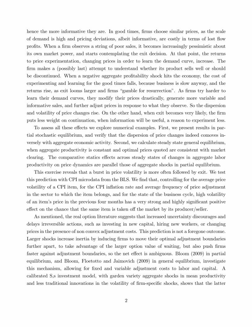
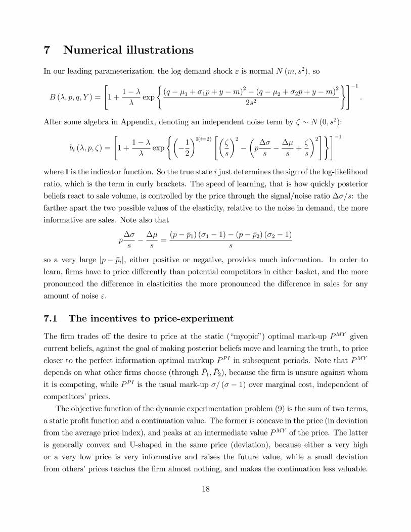
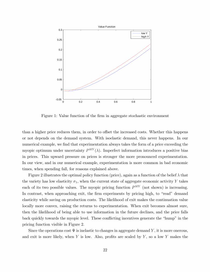
Figure 1 shows the value function V (�; Y ) of the �rm�s problem as a function of the belief

� that the variety has low elasticity �1, when the current state of aggregate economic activity

Y takes each of its two possible values. As mentioned, the value is convex, the upper envelope

of a smooth increasing and convex function W and the zero outside option when choosing exit,

which occurs where the W = 0.

As mentioned, the �rm can learn by choosing a large deviation of its own price from the

rescaled price indices �pi. Given the structure of preferences, under perfect information a �rm

of type 1 only cares about �p1 (and vice versa): only �p1 is relevant to the �rm�s decisions,

any change in the other price index �p2 will only reduce proportionally the real income spent

on basket 2, leaving spending on each basket unchanged. With imperfect information, the

�rm knows both values of �p1 and �p2 in equilibrium, but not which one is relevant to its sales.

Therefore, it can learn by quoting a price that is very high or very low relative to either price

index �pi, unless �p1 and �p2 are very di¤erent. To a �rst approximation, the e¤ect of a drastic

price change on learning only depends on its size and not on its sign: note that the leading term

in (7) is (p��=s)2 for jpj large. A very high price (p > 0), though, enjoys a unique advantage:it reduces sales, thus production costs. A low price (p < 0) must raise revenues much faster

21

0 0.2 0.4 0.6 0.8 1­0.05

0

0.05

0.1

0.15

0.2

0.25

0.3Value Function

low Yhigh Y

Figure 1: Value function of the �rm in aggregate stochastic environment

than a higher price reduces them, in order to o¤set the increased costs. Whether this happens

or not depends on the demand system. With isoelastic demand, this never happens. In our

numerical example, we �nd that experimentation always takes the form of a price exceeding the

myopic optimum under uncertainty PMY (�). Imperfect information introduces a positive bias

in prices. This upward pressure on prices is stronger the more pronounced experimentation.

In our view, and in our numerical example, experimentation is more common in bad economic

times, when spending fall, for reasons explained above.

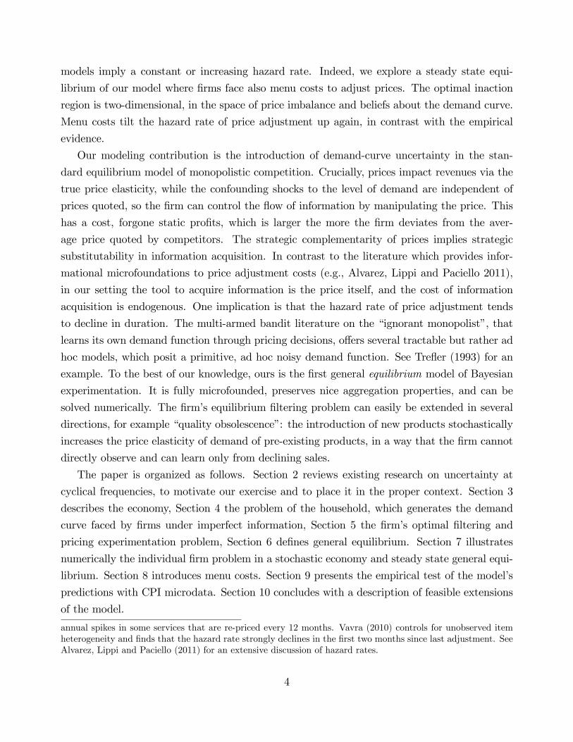
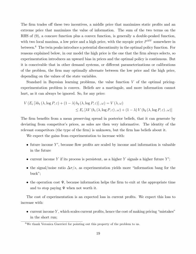
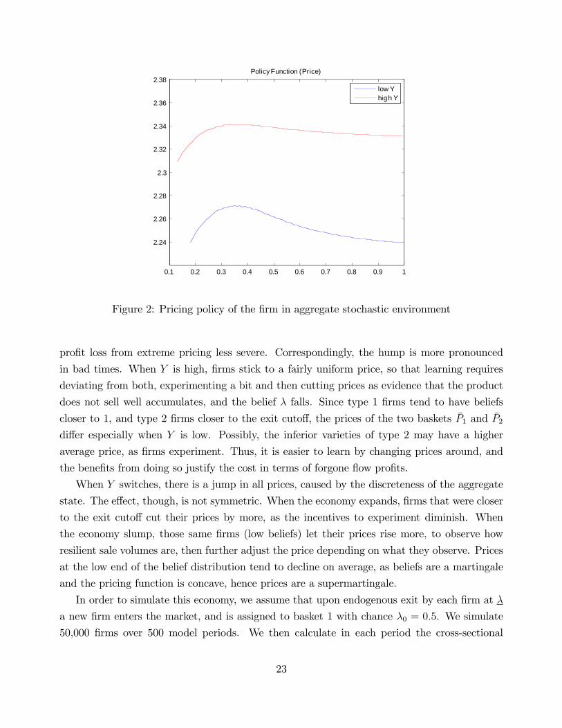
Figure 2 illustrates the optimal policy function (price), again as a function of the belief � that

the variety has low elasticity �1, when the current state of aggregate economic activity Y takes

each of its two possible values. The myopic pricing function PMY (not shown) is increasing.

In contrast, when approaching exit, the �rm experiments by pricing high, to �read�demand

elasticity while saving on production costs. The likelihood of exit makes the continuation value

locally more convex, raising the returns to experimentation. When exit becomes almost sure,

then the likelihood of being able to use information in the future declines, and the price falls

back quickly towards the myopic level. These con�icting incentives generate the �hump�in the

pricing function visible in Figure 2.

Since the operations cost is inelastic to changes in aggregate demand Y , it is more onerous,

and exit is more likely, when Y is low. Also, pro�ts are scaled by Y , so a low Y makes the

22

0.1 0.2 0.3 0.4 0.5 0.6 0.7 0.8 0.9 1

2.24

2.26

2.28

2.3

2.32

2.34

2.36

2.38Policy Function (Price)

low Yhigh Y

Figure 2: Pricing policy of the �rm in aggregate stochastic environment

pro�t loss from extreme pricing less severe. Correspondingly, the hump is more pronounced

in bad times. When Y is high, �rms stick to a fairly uniform price, so that learning requires

deviating from both, experimenting a bit and then cutting prices as evidence that the product

does not sell well accumulates, and the belief � falls. Since type 1 �rms tend to have beliefs

closer to 1, and type 2 �rms closer to the exit cuto¤, the prices of the two baskets �P1 and �P2di¤er especially when Y is low. Possibly, the inferior varieties of type 2 may have a higher

average price, as �rms experiment. Thus, it is easier to learn by changing prices around, and

the bene�ts from doing so justify the cost in terms of forgone �ow pro�ts.

When Y switches, there is a jump in all prices, caused by the discreteness of the aggregate

state. The e¤ect, though, is not symmetric. When the economy expands, �rms that were closer

to the exit cuto¤ cut their prices by more, as the incentives to experiment diminish. When

the economy slump, those same �rms (low beliefs) let their prices rise more, to observe how

resilient sale volumes are, then further adjust the price depending on what they observe. Prices

at the low end of the belief distribution tend to decline on average, as beliefs are a martingale

and the pricing function is concave, hence prices are a supermartingale.

In order to simulate this economy, we assume that upon endogenous exit by each �rm at �

a new �rm enters the market, and is assigned to basket 1 with chance �0 = 0:5. We simulate

50,000 �rms over 500 model periods. We then calculate in each period the cross-sectional

23

standard deviation of price changes. Price changes, and particularly price cuts sliding �o¤ the

hump�on either side of the peak, are more frequent in bad economic times. We �nd that this

measure of price change dispersion has a correlation of about �0:38 with aggregate economicactivity Y . Berger and Vavra (2010) report correlations around �0:4 between the interquartilerange of the monthly changes in CPI components and detrended industrial production. In

our model, revenues and output are proportional to prices, so a standard deviation in % price

changes translates directly into one of sales and output changes.

7.3 Steady state general equilibrium

We now assume that aggregate labor productivity is constant at z = 1. We now have to provide

a full calibration of the economy, because we longer treat output and price indices as exogenous

state variables. Let � denote the chance of exogenous exit, which can be absorbed into the

discount factor to solve the �rm�s experimentation problem in partial equilibrium, but must be

set separately in general equilibrium to compute the out�ow of �rms.

� � �1 �2 � �0 V ar (e") H:99 :02 8 10 1 :4 :1 :0367 :33

We require that aggregate employment equals 1/3 (of available time), and iterate over the cost

of e¤ort parameter �. Speci�cally, we proceed as follows:

1. guess values for �; �P1 and �P2; calculate the resulting value of aggregate output Y and

employment H from market-clearing in the output market and from the labor supply

equation (2);

2. solve the �rm problem in steady state, and �nd the optimal pricing policy;

3. simulate the history of 50,000 �rms, starting from a degenerate distribution of beliefs at

�0; at each step, replace each �rm that exits either exogenously or endogenously with a

new �rm; assign to this new �rm type �1 with chance �0;

4. stop the simulation when the distribution of beliefs settles in both measure of �rms active

for each type and distribution of beliefs by type; compute aggregate employment and

price indices �Pi adding across �rms the simulated prices and resulting employment from

the last round of the simulation;

5. if price indices equal the guess from step 1 and employmentH equals 0.33, stop; otherwise,

update � (in the direction of H � 0:33) and go back to step 1 with the new price indices.

24

0 0.1 0.2 0.3 0.4 0.5 0.6 0.7 0.8 0.9 11.1

1.105

1.11

1.115

1.12

1.125

1.13

1.135

1.14

1.145

z=1z=0p995

Figure 3: Steady state optimal pricing policy for two values of aggregate TFP

After �nding equilibrium for z = 1; we �x the resulting value of work disutility � and

repeat the exercise for z = 0:995; this time iterating over employment H rather than preference

parameter �, until H converges to a steady state value (below 0.33).

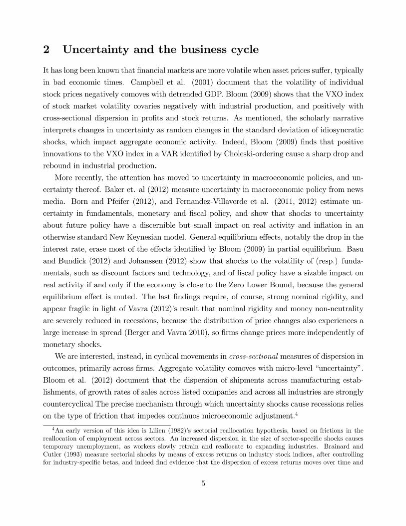
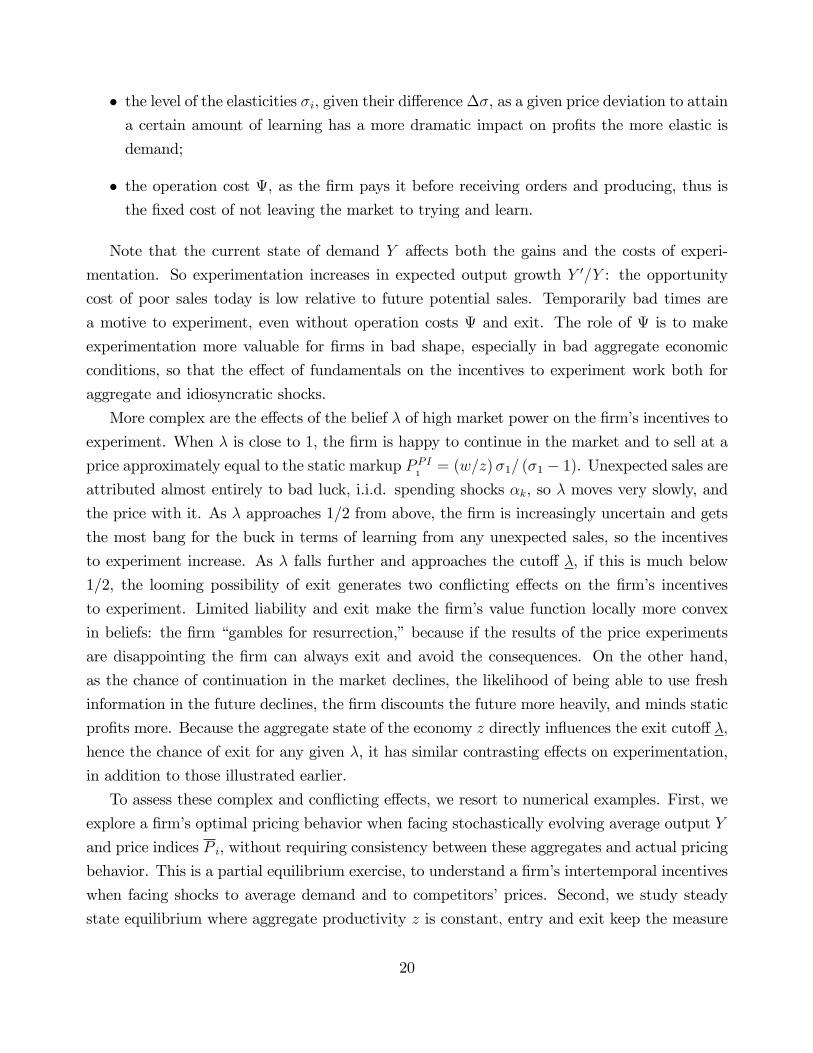
Figure 3 illustrates the pricing policy and exit cuto¤ for each aggregate state. Because the

shocks are to aggregate labor productivity, good prices in units of labor and exit cuto¤ are both

countercyclical. The hump near the exit cuto¤, albeit much less prominent than in the partial

equilibrium exercise, is still visible, and we veri�ed numerically that it is more pronounced

in the low aggregate state. For larger beliefs, the quoted price is very close to their myopic

optimal value. Barring the cyclical e¤ects described earlier, in steady state the only reason to

experiment is the desire to price according to the true demand elasticity, including the option

of exit should demand turn out to be elastic.

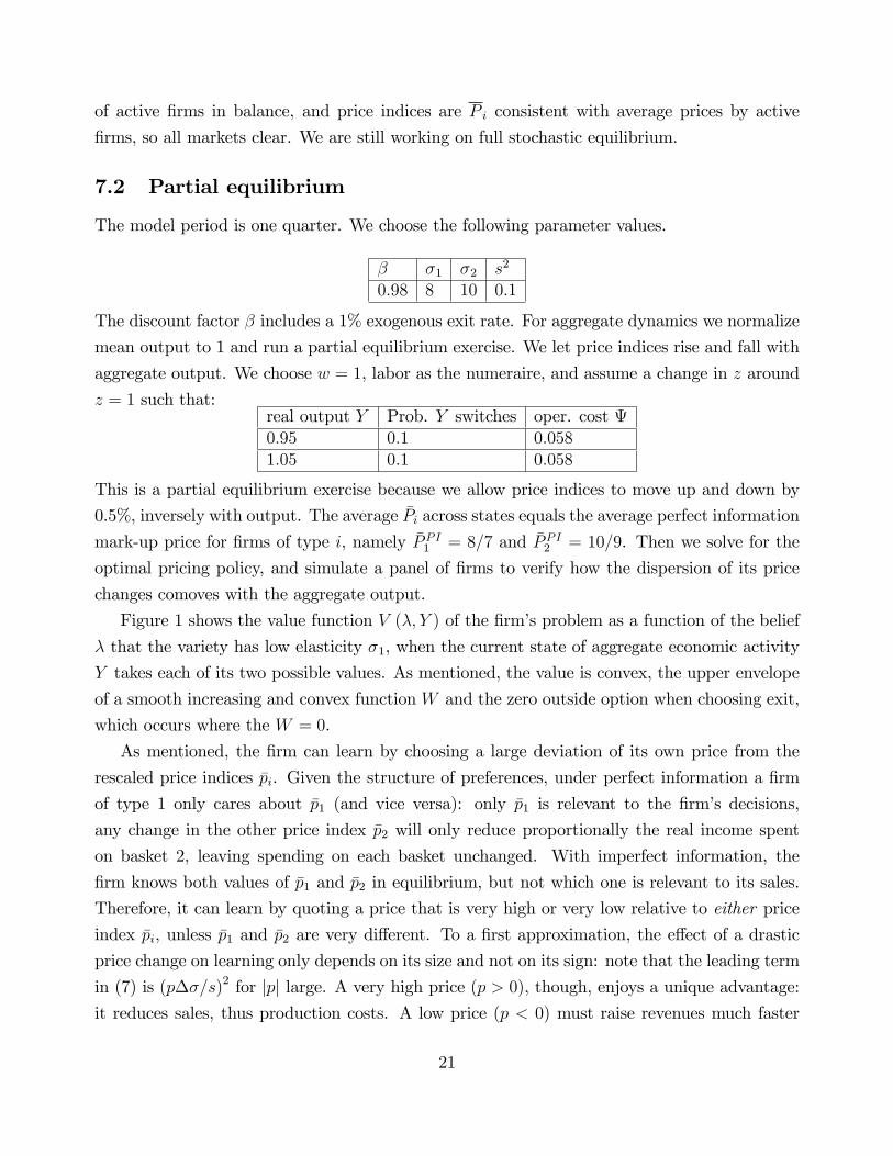
7.4 Hazard rate of price changes

To conclude this section, we study another testable prediction of the model, the hazard rate

of price changes. In both CPI and scanner data, it is well-known that prices are constant

for months at a time, with the median price duration exceeding six months, depending on

the treatment of sales, and the hazard rate of a price change is declining with price duration

(Nakamura and Steinsson 2008), even, crucially, when eliminating cross-item heterogeneity in

25

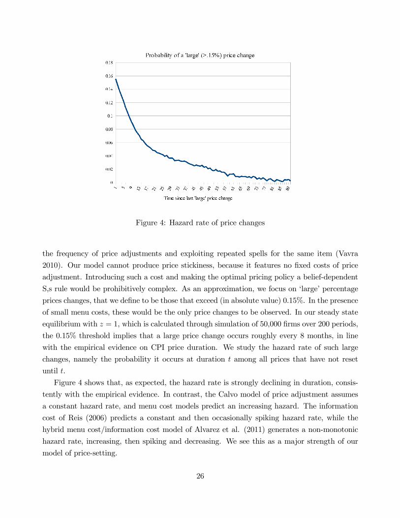
Figure 4: Hazard rate of price changes

the frequency of price adjustments and exploiting repeated spells for the same item (Vavra

2010). Our model cannot produce price stickiness, because it features no �xed costs of price

adjustment. Introducing such a cost and making the optimal pricing policy a belief-dependent

S,s rule would be prohibitively complex. As an approximation, we focus on �large�percentage

prices changes, that we de�ne to be those that exceed (in absolute value) 0.15%. In the presence

of small menu costs, these would be the only price changes to be observed. In our steady state

equilibrium with z = 1, which is calculated through simulation of 50,000 �rms over 200 periods,

the 0.15% threshold implies that a large price change occurs roughly every 8 months, in line

with the empirical evidence on CPI price duration. We study the hazard rate of such large

changes, namely the probability it occurs at duration t among all prices that have not reset

until t.

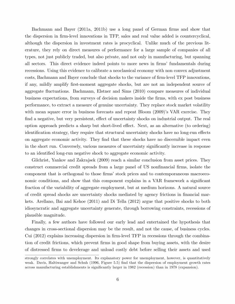
Figure 4 shows that, as expected, the hazard rate is strongly declining in duration, consis-

tently with the empirical evidence. In contrast, the Calvo model of price adjustment assumes

a constant hazard rate, and menu cost models predict an increasing hazard. The information

cost of Reis (2006) predicts a constant and then occasionally spiking hazard rate, while the

hybrid menu cost/information cost model of Alvarez et al. (2011) generates a non-monotonic

hazard rate, increasing, then spiking and decreasing. We see this as a major strength of our

model of price-setting.

26

7.5 Stochastic general equilibrium

[Under construction.]

8 A monetary model with menu costs and price experi-mentation

So far we have treated labor as the numeraire, so all prices we refer to are relative prices.

The attention of the literature, and the empirical evidence we presented, pertain, however, to

nominal prices. As mentioned, our model cannot generate persistent exact price stickiness.

To amend both, we show how to introduce money and menu costs in our model. The goal is

to generate a declining hazard rate of genuine price changes. Intuitively, a �rm is reluctant

to change its price continuously, because of adjustment (menu) costs. When the �rm does

change the price, it can set it optimally so as to maximize pro�ts but also to acquire valuable

information about the demand curve it faces. Typically, the �rst sales observed after the

price change will contain an element of surprise. As the �rm re�nes its estimate of demand

elasticity, the likelihood rises of a further price change, to take advantage of the new information.

Conversely, when a price has been constant for a long time, it is likely that the �rm knows its

demand elasticity well, and does not need to change the price further. Hence, the declining

hazard rate of price changes with duration that we observe in the data is the result of selection

by unobservables (beliefs about the demand curve). The presence of menu costs, however, makes

price adjustment infrequent and optimal, so especially unlikely right after an adjustment.

Preferences and information structure are as before. Money is the numeraire. P is the

nominal price of the variety produced by the �rm, �Pi is the price index of basket i = 1; 2:

Money supply follows

logM 0 = � + � logM + �

where � is an i.i.d. shock.

At each point in time, the consumer optimally allocates half of expenditure to each basket

i = 1, so�P1C1 = �P2C2 =

M

2:

Let the ideal price index

P � =p�P1 �P2:

which equates real spending M=P � to indirect utility. For simplicity, we �x the real wage to w

in utility units through a perfectly elastic labor supply. We also dispose of the �xed operation

27

cost , and introduce a menu cost �, in labor units, a �xed cost that must be paid to change

the current nominal price.

To make the �rm DP problem stationary, we de�ne detrended money supply and prices

m :=M

M0 (1 + �)t ; p :=

P

M0 (1 + �)t ; �pi :=

�Pi

M0 (1 + �)t

Note that these are not real variables, but nominal variables in deviations from a nominal trend.

It is easy to show that Bayes rule is identical to the stationary case with detrended prices

(updating only depends on relative prices, obviously). Using these de�nitions and equalities,

we express �ow pro�ts in real terms

���; P; �P1; �P2;M

�=

M

2p�P1 �P2

��P��1

�P 1��11

+ (1� �) P��2

�P 1��22

��P � w

p�P1 �P2

�as a function of nominal detrended variables:

=m

2

"�1

�p1

�p

�p1

���1+ (1� �) 1

�p2

�p

�p2

���2#� pp�p1�p2

� w�

We now turn to the �rm�s DP problem. The timing is as follows. The �rm enters the period

with previously quoted price P , belief �, and last period�s prices of the two baskets �Pi and

money supply M . Then a new draw of money supply M 0 is observed by all �rms, who then

choose whether to change the price or not, P possibly changes to P 0 and �Pi to �P 0i , each �rm

observes its own sales, collects pro�ts, updates beliefs. So today�s pro�ts and updating depend

on M 0, P 0 and �P 0i .

Detrended money supply follows

logm0 = � logm+ �

Given the state (�; p; �p1; �p2;m) in detrended terms, let V (�; p; �p1; �p2;m) be the value function

of the �rm at the beginning of the period, before the new money supply m0 is drawn, �rms

adjust prices and then update beliefs. LetW (�; p0; �p01; �p02;m

0) be the value of the �rm after �rms

observem0, quote detrended prices p0 and �p01; �p02, but before they observe sales and update beliefs.

Remember that � is the expected pro�t function, given current belief �. So W is the value of

the �rm after new prices are quoted and before customers react. Note that, after updating � to

the new belief �0 = B (�; p0; �p01; �p02; �) through bayes rule B, the vector (�

0; p0; �p01; �p02;m

0) becomes

the state at the beginning of next period. Then

W (�; p0; �p01; �p02;m

0) = � (�; p0; �p01; �p02;m

0)

28

+�E� [�V (b1 (�; p0; �p01; �p

02; �) ; p

0; �p01; �p02;m

0) + (1� �)V (b2 (�; p0; �p01; �p02; �) ; p0; �p01; �p02;m0)]

and the Bellman equation is

V (�; p; �p1; �p2;m) = Em0

�max

�W

��;

p

1 + �; �p01; �p

02;m

0�;max

p0W (�; p0; �p01; �p

02;m

0)� ���

If the �rm does not pay the menu cost � to adjust the nominal, undetrended price P , the

detrended price p declines by an amount equal to the trend in�ation rate �.

8.1 Steady state

We compute general equilibrium when money growth is constant at � and experiences no shocks.

The algorithm proceeds by guessing values for the price indexes of the two baskets �P1 and �P2,

solves the �rm�s DP problem, simulates a large panel of �rms, including entry and exit, and

computes the implied average prices of �rms in each basket, which provide an update for �P1and �P2. Iterating until converges yields the desired equilibrium.

The �rm�s DP problem generates an optimal sS policy in two dimensions: old price P and

belief � about demand elasticity. The �rm is more willing to change its price the farthest it

is from the optimal price, given current beliefs, and the less extreme beliefs are, because then

price changes yield more valuable information.

We now present, by way of illustration, results from a fully computed stationary general

equilibrium, where price indexes have converged to initial guesses. For simplicity, we eliminate

endogenous exit and allow only for exogenous exit with probability �, and we make labor supply

in�nitely elastic, �xing the real wage at a normalized value of 1. The rest of the parameter

values are:� � �1 �2 � �0 V ar (e") � �:99 :02 8 10 1 :4 :1 0 :02 :01

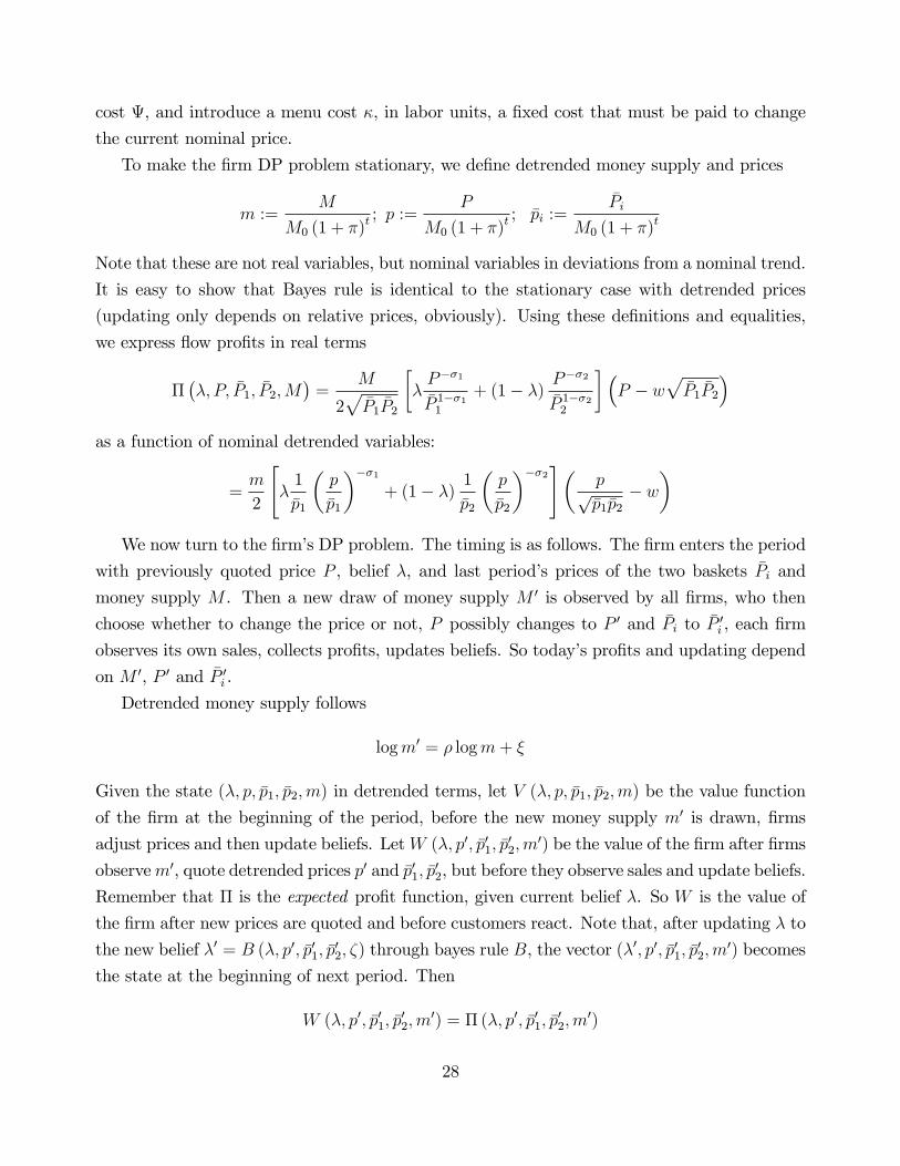
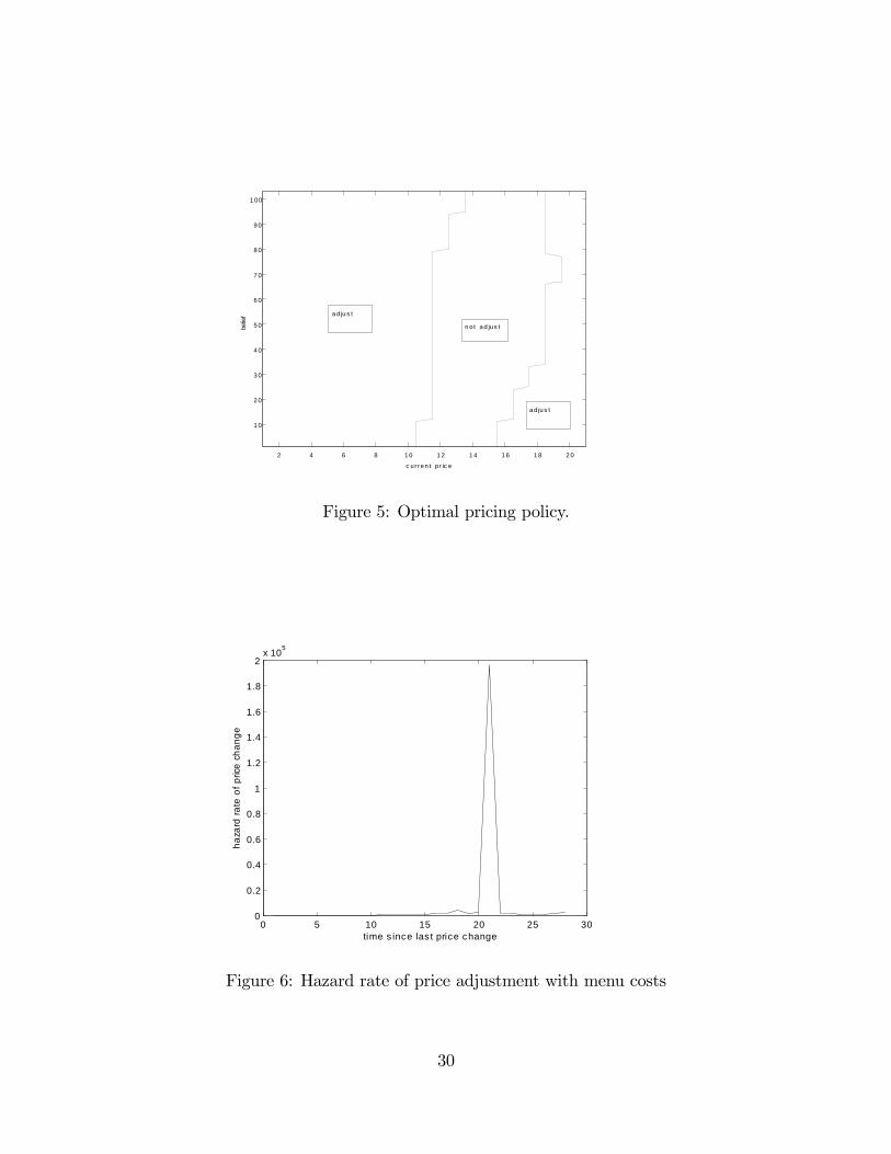
Figure 5 shows the optimal band policy. If beliefs are either 0 or 100 (%) that the state is

1, then we are back to perfect information and obtain a standard sS policy. The optimal price

increases with the belief because the mark-up is higher, so bands are skewed to the right. The

width of the bands is higher for intermediate beliefs, because there news from realized sales

matter more, beliefs move faster, so the larger variance of belief changes induces a standard

option value of waiting e¤ect.

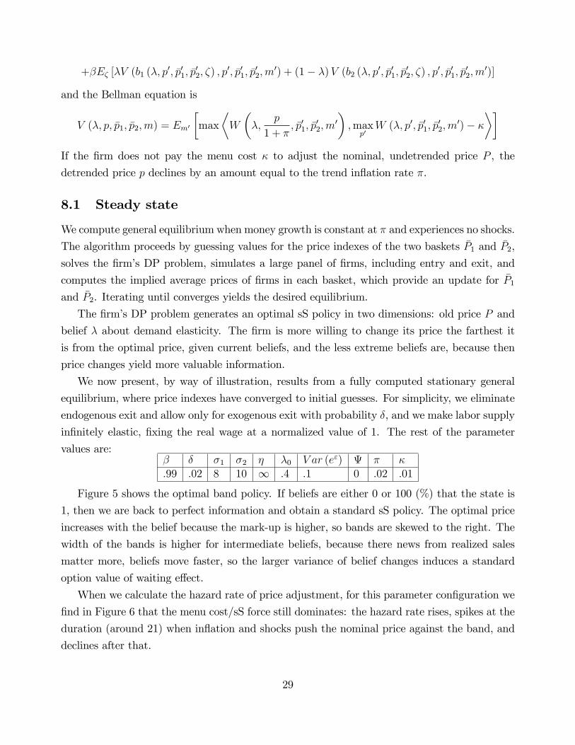
When we calculate the hazard rate of price adjustment, for this parameter con�guration we

�nd in Figure 6 that the menu cost/sS force still dominates: the hazard rate rises, spikes at the

duration (around 21) when in�ation and shocks push the nominal price against the band, and

declines after that.

29

c ur ren t   p r ic e

belie

f

2 4 6 8 1 0 1 2 1 4 1 6 1 8 2 0

1 0

2 0

3 0

4 0

5 0

6 0

7 0

8 0

9 0

1 00

n ot   ad jus t

a d ju s t

a d ju s t

Figure 5: Optimal pricing policy.

0 5 10 15 20 25 300

0.2

0.4

0.6

0.8

1

1.2

1.4

1.6

1.8

2x 105

time s ince las t price change

haza

rd ra

te o

f pric

e ch

ange

Figure 6: Hazard rate of price adjustment with menu costs

30

This exercise highlights a tension between data and models. In the data, nominal prices

stay exactly constant for months at a time, strongly suggesting some form of menu costs. The

same menu costs, however, imply that the prices that do change tend to be �old�, because far

from the target. This is the essence of state-dependent pricing. In the data, however, most

prices that change are young, they changed recently. It seems arduous to generate a declining

hazard, as observed in the data, in a rational model without some form of learning. It must be

the case that the act of changing a price alters the information set of the �rm (which is what

learning means), and that triggers a further change. If the information set did not change, the

�rm would not want to pay the menu cost twice in a row. Without menu costs, it would change

prices all the time. We are currently exploring whether for extremely small menu costs the

learning e¤ect dominates at short durations and the menu cost at long durations, where prices

are set under very accurate information.

9 Empirical evidence from CPI microdata

In the model without menu costs, price volatility should fall with time since entry (age of the

�rm), due to a standard selection e¤ect common to all learning models. Firms that survive a

long time must have been persuaded by a long series of strong sales to be facing a high level

and a low elasticity of demand. Any additional piece of news has a negligible impact on this

belief, either way, because it adds little to the previously accumulated evidence. As the optimal

policy function maps directly beliefs into price, and is approximately linear at high beliefs, it

follows that price volatility declines with �rm age.

The shape of the optimal policy also suggests that all �rms, even if old, should experience a

burst in price volatility when they are in trouble, including when the economy is in a recession.

The reason is twofold: �rms experiment more with their price when close to giving up and

leaving the market, thus generate more movement in beliefs, and the policy function has more

curvature at low beliefs. Therefore, a sudden burst of price volatility should predict exit.

We explore empirically this correlation on monthly price observations on the Entry-Level

Items (ELIs), such as �beverages�, that the Bureau of Labor Statistics collects to form the

Consumer Price Index. We restrict attention to non-durable goods and services. Each ELI

price is the average of many price observations in various stores for individual varieties of the

ELI, such as �Coca Cola six-pack�. We identify a model �rm with a single item product in the

data. We specify a logit for the chance that the items exits, namely it is no longer found to be

available for sale, as a function of (subsets of) the following variables: the standard deviation of

price growth rates for that item over the previous four months (v̂4), which should predict exit;

31

the standard deviation of price growth rates for the ELI to which the item belongs since the

ELI �rst appeared (v̂), to control for the average variability of the price of that type of product

or service; a monthly recession dummy (R), according to NBER�s business cycle dating, and

its interaction with v̂4; the frequency of adjustment (f4) of that item�s price in the last four

months; and two controls relating to the 2-digit sector to which the ELI belongs, namely the

sector-speci�c average CPI in�ation rate (�SECT ) and average frequency of price adjustment

(fSECT ). Finer sectorial classi�cations exist in the data but are di¢ cult to implement for this

speci�cation. The data cover 1988-2010. Overall we have 2,971,175 item-month observations.

For details, see Berger and Vavra (2010).

Table 1 reports the results. Standard errors are in parentheses. Estimates are very accurate

thanks to the huge sample size. All speci�cations include controls at the sector level. In

isolation, recent price volatility (v̂4) predicts a lower probability of exit (column I), the opposite

of what the model indicates. The negative estimated coe¢ cients on v̂4 in speci�cations I-II

is due entirely (and more) to unobserved heterogeneity across items. When we control for

the frequency of price changes of that item in the last four months (f4) in (II), the estimated

coe¢ cients on v̂4 remains negative but is cut in half. When we control for the the overall

volatility v̂ of price changes for the ELI to which the item belongs to since the beginning of

the sample (or since the ELI entered the CPI basket, whichever happens later), the estimated

coe¢ cient on v̂ is so large and negative that the estimated coe¢ cient of v̂4 turns positive,

without (III) or with (IV) the cyclical interaction variable v̂4�R: In other words, items whoseprice is less sticky, in frequency or actual size of price changes, even controlling for the same

characteristics at the sectorial level, are items that are much more likely to remain in the CPI

for a longer time. When we control for unobserved heterogeneity with both f4 and v̂ (V-VI),

the positive e¤ect of recent price volatility on exit grows even larger, and the cyclical interaction

v̂4�R preserves its positive sign. When we introduce the recession dummy R alone (VII-VIII),it has the expected strong positive e¤ect on the probability of exit, and the interaction term with

recent price volatility is no longer statistically signi�cant, so most of the e¤ect of the business

cycle shows up as a direct impact. But the strong predictive power of recent idiosyncratic price

volatility on exit is robust and, if anything, stronger.

The reason why the two measures of price stickiness, frequency f4 and size v̂ of log price

changes, play di¤erent roles presumably is that the latter may be large also with rare, but huge,

price changes. All estimated coe¢ cients, except as discussed that of v̂4, remain quite stable in

size across speci�cations. To interpret the size of an estimated logit coe¢ cient, for example,

in column VI, when the standard deviation of log price changes v̂4 goes up by one percentage

point, the relative likelihood of forced substitution of the item goes up by multiplicative factor

32

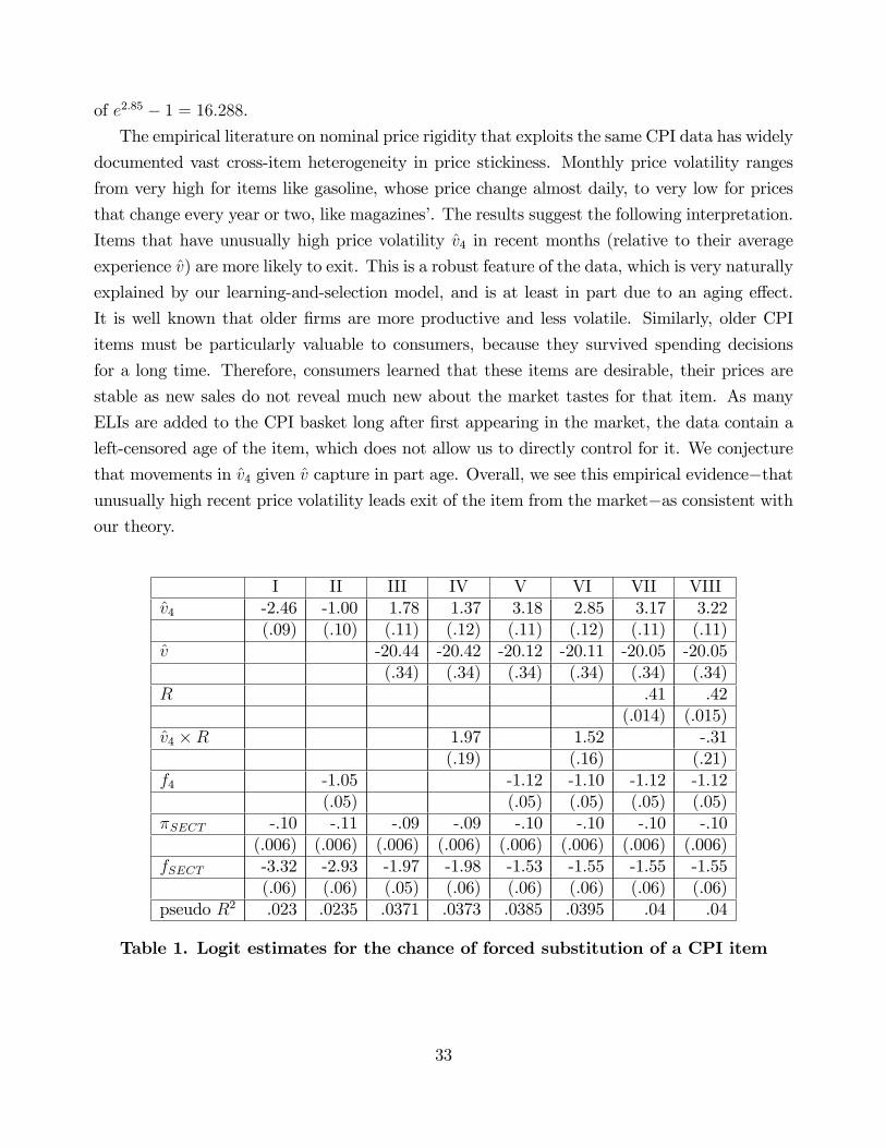
of e2:85 � 1 = 16:288.The empirical literature on nominal price rigidity that exploits the same CPI data has widely

documented vast cross-item heterogeneity in price stickiness. Monthly price volatility ranges

from very high for items like gasoline, whose price change almost daily, to very low for prices

that change every year or two, like magazines�. The results suggest the following interpretation.

Items that have unusually high price volatility v̂4 in recent months (relative to their average

experience v̂) are more likely to exit. This is a robust feature of the data, which is very naturally

explained by our learning-and-selection model, and is at least in part due to an aging e¤ect.

It is well known that older �rms are more productive and less volatile. Similarly, older CPI

items must be particularly valuable to consumers, because they survived spending decisions

for a long time. Therefore, consumers learned that these items are desirable, their prices are

stable as new sales do not reveal much new about the market tastes for that item. As many

ELIs are added to the CPI basket long after �rst appearing in the market, the data contain a

left-censored age of the item, which does not allow us to directly control for it. We conjecture

that movements in v̂4 given v̂ capture in part age. Overall, we see this empirical evidence�thatunusually high recent price volatility leads exit of the item from the market�as consistent withour theory.

I II III IV V VI VII VIIIv̂4 -2.46 -1.00 1.78 1.37 3.18 2.85 3.17 3.22

(.09) (.10) (.11) (.12) (.11) (.12) (.11) (.11)v̂ -20.44 -20.42 -20.12 -20.11 -20.05 -20.05

(.34) (.34) (.34) (.34) (.34) (.34)R .41 .42

(.014) (.015)v̂4 �R 1.97 1.52 -.31

(.19) (.16) (.21)f4 -1.05 -1.12 -1.10 -1.12 -1.12

(.05) (.05) (.05) (.05) (.05)�SECT -.10 -.11 -.09 -.09 -.10 -.10 -.10 -.10

(.006) (.006) (.006) (.006) (.006) (.006) (.006) (.006)fSECT -3.32 -2.93 -1.97 -1.98 -1.53 -1.55 -1.55 -1.55

(.06) (.06) (.05) (.06) (.06) (.06) (.06) (.06)pseudo R2 .023 .0235 .0371 .0373 .0385 .0395 .04 .04

Table 1. Logit estimates for the chance of forced substitution of a CPI item

33

10 Extensions and conclusions

It is plausible that the demand elasticity � changes stochastically, unobserved by the �rm (other

than through noisy sales). We envision the following process. New varieties are introduced each

period. For example, the iPhone, when �rst introduced, may have been considered similar to a

Blackberry. Sales (and stock market) then revealed that this was not the case, and the iPhone

was quite a unique device. New smartphones introduced later, however, may or may not be

close substitutes for the iPhone. Only sales data will tell. Therefore the true elasticity � has a

positive drift, which may depend on the amount of entry. Given the Kalman-�lter-like structure

of our observation equation (5), this extension is straightforward to implement. It describes

well a product life cycle.

A Appendix

A.1 Proof of Proposition 1

The myopic optimal price maximizes expected static pro�ts, that we denote by �MY :We show

that �MY is supermodular in P; � at least near the optimizer PMY . Taking a derivative w.r.

to �

@�MY (P; �)

@�=

�P � w

z

� Y2

�P��1

�P 1��11

� P��2

�P 1��22

�

=�MY (P; �) + �

�P � w

z

�P��2�P1��22

Y=2

�Y=2=

2

�Y

��MY (P; �)� �MY (P; 0)

�Supermodularity of �MY (P; �) is equivalent to this function being increasing in P at P =

PMY (�). Taking another derivative w.r. to P , evaluating it at PMY (�) and using the fact

that, by de�nition, PMY (�) maximizes �MY (P; �) ;�@2�MY (P; �)

@�@P

�P=PMY (�)

= � 2

�Y

d

dP

��MY (P; 0)

�P=PMY (�)

By concavity of �MY (P; 0) in P; this is positive if and only if the optimal price exceeds the one

chosen under perfect information at � = 0: PMY (�) > PMY (0) = P PI2 : We draw the following

conclusion:dPMY (�)

d�> 0, PMY (�) > PMY (0) :

The last inequality is true at � = 1 because PMY (1) = P PI1 > P PI2 = PMY (0) by �2 > �1.

By continuity, it is true for � large enough. By contradiction, if for some �0 > 0 we have

PMY (�0) = PMY (0), then either PMY (�0 ��) > PMY (0) for � > 0 small enough, but

34

this requires dPMY (�0��)d�

< 0, which contradicts the equivalence above; or PMY (�0 ��) =PMY (0) over an open interval of small positive values of �, but this equality cannot hold on

an interval by the strict concavity of expected pro�ts; or PMY (�0 ��) < PMY (0), but thendPMY (�0)

d�< 0 for all � 2 (0; �0), thus PMY (�) keeps declining with � # 0 and stays below

PMY (0), until PMY (0+) < PMY (0). But, by the Theorem of the Maximum, the optimizer

PMY (�) is continuous, which yields the �nal, desired contradiction.

A.2 Bayesian updating with log-Normal preference shocks

Assume " = log� � N (m; s2). The log-Likelihood Ratio (log-LR) of state 2 to state 1 is, in

state i = 1 (when q = �1 � �1p+ y + "),

("�m)2 � (�1 � �1p+ "� �2 + �2p�m)2

2s2=�̂2 �

��̂ ���+ p��

�22s2

where �̂ = "�m � N (0; s2), and

�� = �2 � �1�� = �2 � �1

Similarly, in state 2 (when q = �2 � �2p+ y + ") the log-LR is

(�2 � �2p+ "� �1 + �1p�m)2 � ("�m)2

2s2

=

���� p�� + �̂

�2� �̂2

2s2=

���̂ ���+ p��

�2� �̂2

2s2

Let~� = ��̂ = m" � " � N

�0; s2

�so the log-LR in state 2 is�

~� ���+ p���2���~��2

2s2=

�~� ���+ p��

�2� ~�2

2s2:

If we let � � N (0; s2) denote a generic random variable independent of the state, the log-LR

in each state is the same random variable except that the state i causes a sign switch:

(�1)I(i=2) �2 � (��p���+ �)2

2s2:

where I is the indicator function. That is, ~� and �̂ have the same distribution, independent ofthe state, that we capture through �.

35

ReferencesAlvarez, F., F. Lippi and L. Paciello, 2011, �Optimal price setting with observation and

menu costs�, Quarterly Journal of Economics, 126, pp. 1909-1960.

Arellano, C., Y. Bai, P. Kehoe, 2012, �Financial Markets and Fluctuations in Uncertainty�,

Minneapolis FED Research Department Sta¤ Report 466.

Bachmann, R. and C. Bayer, 2011a, �Investment Dispersion and the Business Cycle�, NBER

WP 16861.

Bachmann, R. and C. Bayer, 2011b, �Uncertainty Business Cycles - Really?�, NBER WP

16862.

Bachmann, R., S. Elstner, and E. Sims, 2010, �Uncertainty and Economic Activity: Evi-

dence from Business Survey Data�, NBER WP 16143. Forthcoming in the American Economic

Journal: Macroeconomics.

Baker, Scott, Nicholas Bloom, and Steven J. Davis. 2012. �Measuring Economic Policy

Uncertainty�, mimeo, Stanford University.

Berger, D. and J. Vavra, 2010, �Dynamics of the U.S. Price Distribution�, mimeo NWU

and U Chicago.

Bloom, N., 2009, �The Impact of Uncertainty Shocks�, Econometrica, May.

Bloom, N., M. Floetotto, N. Jaimovich, I. Saporta-Eksten, S. Terry, 2012, �Really Uncertain

Business Cycles�, NBER WP 18245.

Born, B. and J. Pfeifer, 2012, �Policy Risk and the Business Cycle�, mimeo U Mannheim.

Brainard, L. and D. Cutler, 1993, �Sectoral Shifts and Cyclical Unemployment Revisited�,

Quarterly Journal of Economics.

Campbell J.Y, M. Lettau, B. Malkiel and Y. Xu, 2001, �Have Individual Stocks Become

More Volatile? An Empirical Exploration of Idiosyncratic Risk�, Journal of Finance 56(1),

1-41.

Cui, W. 2012, �Delayed Capital Reallocation�, mimeo Princeton University.

Campbell, J. R. and B. Eden, 2010, �Rigid Prices: Evidence from U.S. Scanner Data�, July

2010, WP 2005-08

Davis, S., J. Haltiwanger and S. Schuh, 1996, Job Creation and Destruction, MIT Press.

D�Erasmo, P. and H. Moscoso Boedo, 2012, �Intangibles and Endogenous Firm Volatility

over the Business Cycle�. mimeo University of Virginia

Di Tella, S., 2012, �Uncertainty Shocks and Balance Sheet Recessions�, mimeo MIT.

Fernandez-Villaverde, J., P. Guerron-Quintana, J. Rubio-Ramirez, nd Martin Uribe, 2011,

�Risk Matters: The Real E¤ects of Stochastic Volatility Shocks�, American Economic Review,

101: 2530-61.

36

Fernandez-Villaverde, J., P. Guerron-Quintana, K. Kuester, J. Rubio-Ramirez, 2012 �Fiscal

Volatility Shocks and Economic Activity�, mimeo.

Gilchrist, S., V. Yankov and E. Zakrajsek, 2009, �Credit market shocks and economic �uc-

tuations: Evidence from corporate bond and stock markets�, Journal of Monetary Economics,

56(4), pp. 471-493.

Johannsen, B., 2012, �When are the E¤ects of Fiscal Policy Uncertainty Large?�, mimeo

NWU.

Kotler, P., 2000, Marketing Management, The Millenium Edition, Prentice Hall, Upper

Saddle River, NJ.

Lilien, D.M., 1982, �Sectoral shifts and cyclical unemployment�, Journal of Political Econ-

omy, 90(4), 777-793

Nakamura, E. and J. Steinsson, 2008, �Five Facts About Prices: A Reevaluation of Menu

Cost Models�, Quarterly Journal of Economics, 123(4), 1415-1464.

Tre�er, D., 1993, �The Ignorant Monopolist: Optimal Learning with Endogenous Informa-

tion,�International Economic Review.

Vavra, J., 2010, �The Empirical Price Duration Distribution andMonetary Non-Neutrality�,

mimeo.

Vavra, J., 2012, �In�ation Dynamics and Time-Varying Volatility: New Evidence and an

Ss Interpretation�, mimeo.

37