Universidade Federal do Rio de Janeiro Instituto de Matemática

Laboratór io de Matemát ica Apl icada Departamento de Matemática Aplicada

1

BRAZILIAN MORTALITY AND

SURVIVORSHIP LIFE TABLES

INSURANCE MARKET EXPERIENCE - 2010

Prof. Mário de Oliveira (PhD) – UFRJ

Prof. Ricardo Frischtak (PhD) – UFRJ

Prof. Milton Ramirez (DSc) – UFRJ

Prof. Kaizô Beltrão (PhD) – FGV

Profª. Sonoe Pinheiro (DSc) – IBGE

2

CONTENTS

CHAPTER 1 – INTRODUCTION ................................................................................ 3

CHAPTER 2 – BRIEF HISTORY OF MORTALITY TABLES.................................... 4 CHAPTER 3 – MORTALITY GRADUATION ............................................................ 7

3.1 Introduction ......................................................................................................... 7 3.2 Distributions ........................................................................................................ 8

3.3 Criteria for model choice ................................................................................... 10 CHAPTER 4 – DATABASE CONSTRUCTION ........................................................ 11

4.1 The insured population ...................................................................................... 11 4.2 The TABUAS Database .................................................................................... 12

CHAPTER 5 – SELECTION OF SUBPOPULATIONS.............................................. 17 5.1 Population Distribution and Evolution in Time .................................................. 17

5.2 IBNR Estimates ................................................................................................. 22 5.3 Selection criteria for exclusion of subpopulations .............................................. 23

5.4 Differentiation of mortality curves according to sex and coverage ..................... 29 CHAPTER 6 – CONSTRUCTION OF LIFE AND SURVIVAL TABLES ................. 34

6.1. HELIGMAN & POLLARD Model................................................................... 34 6.2. Methodology for the parameters estimation ...................................................... 42

6.3. Curve fitting ..................................................................................................... 43 CHAPTER 7 – BR-EMS TABLES ............................................................................. 58

7.1 Male Survivorship: BR-EMSsb-v.2010-m ......................................................... 59 7.2 Male Mortality: BR-EMSmt-v.2010-m .............................................................. 62

7.3 Female survivorship: BR-EMSsb-v.2010-f ........................................................ 65 7.4 Female Mortality: BR-EMSmt-v.2010-f ............................................................ 68

7.5 Comparison of BR-EMS with well known tables ............................................... 71 7.6 Examples of the use of BR-EMS tables ............................................................. 79

3

CHAPTER 1 – INTRODUCTION

In the first decade of the present century, the Brazilian life insurance market has

expanded at an accelerated rate. Insurance companies operating in Brazil were using

foreign life tables, since there were no available local life tables.

Consequently, FenaPrevi – the National Federation of Open pension funds and Life

Insurance Companies – commissioned LabMA/UFRJ – the Applied Mathematics Lab

of the Mathematics Institute of Federal University of Rio de Janeiro – to construct life

tables for the Brazilian insurance market.

This project was followed by SUSEP – the Brazilian Supervising Insurance Authority.

The present work describes the methodology used and presents the survival and

mortality tables constructed thereof, based on the experience of the Brazilian insurance

market of life products, for the years 2004, 2005 and 2006. Data was provided by a pool

of Insurance Companies, representing an 82% share of the market.

These life tables were named Experiência do Mercado Segurador Brasileiro, BR-EMS

(Experience of the Brazilian Insurance Market) and consists of four variants for

mortality (male and female) and survivorship (male and female). The variants were

given the following names: BR-EMSsb-v.2010-m, BR-EMSsb-v.2010-f, BR-EMSmt-

v.2010-m e BR-EMSmt-v.2010-f, where “sb” denotes survivorship, “mt” mortality, “m”

male and “f” female.

SUSEP established tables BR-EMS as Standard Life Tables for the Brazilian Insurance

Market. SUSEP also demanded that they are to be reviewed in 2015.

We would like to thank all members of the Actuarial Committee of FenaPrevi who

contributed with suggestions and discussions in all phases of the present work and also

all of our students of LabMA/UFRJ, specially Paulo Vitor da Costa Pereira who was in

charge of redoing all graphs in the book.

4

CHAPTER 2 – BRIEF HISTORY OF MORTALITY TABLES

Life tables exist for a long time in human history. There is evidence that in ancient

Rome, in the 3rd century B.C., the State collected and elaborated statistics of life and

death, probably using life table schemes, calculating life expectancy at birth and other

ages (Duchene & Wunsch, 1988). However, the first scientific references to life tables

occur in the work of John Graunt, “Natural and political observations made upon the

bills of mortality”, published in 1662 (apud David, 1998), and notably the seminal paper

by astronomer Edmond Halley, in 1693 (apud Duchene & Wunsch, 1988) where the

basis of actuarial science were laid.

Since then, numerous tables have been built for different countries and regions, as well

as, tables for specific purposes to subsidize the actuarial work of insurance companies

and pension funds.

Life tables are an important tool to help with the establishment of public policies, such

as, health, education, economic planning, workforce allocation, social security,

insurance in general, and investment planning.

There are two issues when one considers constructing a life table for a specific

population group:

i) The first concerns the data in itself, mostly characteristics of the population at

risk, e.g. age and sex, and statistics of deaths. For example, in Brazil, IBGE

(National Central Statistical Agency) constructs life tables for the population

as a whole, based on census data and deaths from the Civil Registry. It is

well known that there is under-registration of deaths, since not all deaths are

reported appropriately.

Therefore, one usually uses a correction factor to account for this error. The

literature reports several techniques to estimate under-registration (UN,

Manual X, 1983). For instance, it could be a uniform correction for all ages,

or alternatively, specific corrections for certain age groups, such as children

and elderly population. In Brazil, there is evidence of stronger under-

registration for the extreme age-groups, so that one usually should perform

5

corrections differentiated for the extremely young and extremely old age-

groups.

In the present study, though data were administrative records from insurance

companies, LabMA/UFRJ decided to countercheck the death information

with available government data in systems of the Ministério da Previdência

Social (Social Security Administration).

ii) The second issue involves choosing an adequate model to describe the mortality

pattern. For a given age-group (x), deaths can be considered as random

variables with Binomial distributions, B(Nx,qx), with a given size parameter,

Nx, and an unknown probability of death, qx, to be estimated. If the age-

group x is large, one may consider a Poisson approximation to the Binomial.

In this area of knowledge, it is quite common to use non parametric

techniques for estimating the vector probability of death in all ages. In

general these methods involve some kind of smoothing. The UN published

Manual X: Indirect techniques for demographic estimation (1983), where a

family of life tables was established according to different regions of the

world, based on the experience of 158 life tables. These families were

indexed by a single parameter, making their use somehow limited.

On the other hand, there have always been many parametric models for life

tables. The first models were simple mathematical curves, such as the linear

model proposed by DeMoivre. Gompertz (1825) proposed a model based on

the hypothesis of a life force diminishing with age. He defined the life force

as the inverse of the instant mortality rate: 1x , where xxx ll / , hence

solving the differential equation for 1x , 1

1

xx k

dxd

,where k is a positive

constant. Solving for x , one finds xx Bc . From the definition of x in

terms of xl the solution of the differential equation is xcx gll 0 , where g and

c are positive constants.

Later in the 19th century, Makeham generalized Gompertz`s model with the

introduction of a constant factor to the instant mortality rate, independent of

age, to represent deaths by accidents. Models based on Gompertz/Makeham

proposals are still very much popular and proved to produce very good

6

results. It just happens that in many instances, these models are particularly

good for describing mortality for certain age groups, but not for all. For

instance, the model proposed by Heligman and Pollard has a very important

component for middle and old ages which is basically Gompertz/Makeham.

Other authors followed different paths to establish mortality laws. For

instance, the Weibull distribution, which describes the failure pattern of

interacting complex and multiple dynamical systems, may also be used for

human beings.

Still another approach would be to model different age brackets using

specific mortality models. For instance, Heligman and Pollard used three

components, each one dominant in a certain age bracket: children, young

adults and adults.

For all methods used for estimating life tables, one usually starts with a process of

smoothing the crude rates, initially calculated from the raw data, ( xq̂ ) x = 0, 1, 2... In

many cases, crude rates tend to oscillate as a function of age, which is not plausible as a

theoretical model for mortality. Since the ageing process is continuous in time, one

should expect a rather continuous mortality function. Therefore, the true non-observable

parameters of a life table, ( xq~ ), should be continuous as a function of age, and the crude

rates could be considered as sample estimates of these non-observable parameters. The

greater the population, the greater is the precision of estimate.

Graduation can be defined as the set of principles and methods used to smooth the crude

mortality rates to generate a mortality function, presenting desirable features such as

avoiding spikes and depression, as well as being monotone above a certain age.

The analysis of different models for life-tables constitutes an important part of the

present work. The next chapter mentions some of these techniques and analyzes their

pros and cons, converging to the chosen model.

7

CHAPTER 3 – MORTALITY GRADUATION

3.1 Introduction

This chapter covers some graduation methods for mortality tables. The present brief

review is based in the literature, which is listed in the bibliography. Usually the idea is

to obtain a smooth curve of mortality rates, monotonically increasing after a certain age,

typically around 30 years.

There are several possible classifications of graduation methods. The first possibility is

between parametric and nonparametric methods.

Parametric methods are rather efficient, once one can describe the mortality

phenomenon by a set of equations with a given (not too large) number of parameters.

With the right parametric family one can rationalize the mortality behavior of a

population, sometimes by associating the parameters with certain mortality

characteristics.

On the other hand, nonparametric methods are smoothing methods that either directly

transforms crude rates through running averages or medians into a smooth sequence, or

else this kind of sequence is obtained by an optimization process. Parametric and

nonparametric methods can be combined in a complementary fashion, by proceeding

initially with a nonparametric method, which in turn feeds a parametric procedure

(Debón, 2003).

There are several other possible classifications of graduation methods, according to

whether they incorporate or not the time dimension. In what follows, one lists some of

the alternative classifications found in the literature, without the time dimension.

Copas and Haberman (1983) classify the graduation methods which do not involve the

time dimension in three groups:

1. Graphical methods;

2. Parametric methods; and

3. Summation and adjusted-average methods

Benjamin and Pollard (1980) consider 5 large groups:

1. Graphical methods;

8

2. Summation and adjusted-average methods;

3. Graduation methods using mathematical formulae;

4. Graduation by reference to a standard life table; and

5. Osculatory interpolation and splines (abridged and model life tables)

Abid, Kamhawey & Alsalloum (2005) tally actuarial graduation methods into nine

groups, fractioning some of groups mentioned by Copas/Haberman and

Benjamin/Pollard:

1. Graphical method;

2. Summation and adjusted-average methods;

3. Kernel's method;

4. The method of osculatory interpolation;

5. The spline method;

6. The curve fitting or parametric method;

7. Graduation by reference to a standard table;

8. Difference equation method; and

9. Linear programming method.

3.2 Distributions

The most commonly used distributions for modeling deaths and survivors in life table

models for a homogenous population group (same sex and age) are the binomial and the

Poisson distributions. The death of a person can be modeled by a Bernouilli (0,1)

distribution, and the sum of independent Bernouilli distributions is a Binomial

distribution B(Nx, qx), where Nx is the number of living individuals of age x and qx is the

probability of death at age x. The maximum likelihood estimator for qx is given by the

observed mortality rate x

xx N

Oq ˆ . The use of MLE for qx does not guarantee the

smoothness of the curve of xq̂ as function of x. Therefore, one rarely uses these MLEs

directly, but rather employs a smoothing method for the graduation of life tables. This

smoothing process is equivalent to the introduction of constraints in an optimization

process. The probability of death usually concerns a given time interval (most

commonly one year). In a given population, not all individuals are exposed to the risk

for the full year. Nevertheless, an individual exposed during a whole year is equivalent

to n individuals exposed to periods that sum up to one year. The total age group

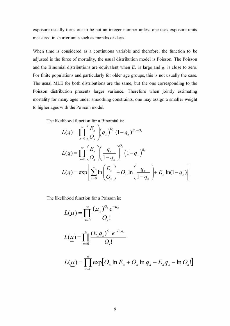
9

exposure usually turns out to be not an integer number unless one uses exposure units

measured in shorter units such as months or days.

When time is considered as a continuous variable and therefore, the function to be

adjusted is the force of mortality, the usual distribution model is Poisson. The Poisson

and the Binomial distributions are equivalent when Ex is large and qx is close to zero.

For finite populations and particularly for older age groups, this is not usually the case.

The usual MLE for both distributions are the same, but the one corresponding to the

Poisson distribution presents larger variance. Therefore when jointly estimating

mortality for many ages under smoothing constraints, one may assign a smaller weight

to higher ages with the Poisson model.

The likelihood function for a Binomial is:

0

0

0

( ) (1 )

( ) 11

( ) exp ln ln ln(1 )1

x x x

xx

w O E Oxx x

x x

Ow Ex x

xx xx

wx x

x x xx xx

EL q q q

O

E qL q qqO

E qL q O E qqO

The likelihood function for a Poisson is:

w

x x

Ox

OeL

xx

0 !)()(

w

x x

qEOxx

OeqEL

xxx

0 !)()(

w

xxxxxxxx OqEqOEOL

0

!lnlnlnexp)(

10

3.3 Criteria for model choice

Due to the intrinsic characteristics of the project that originated this book, the selection

of methodology to be adopted was guided by the following desiderata:

i) parsimony criterion (Ockham’s razor) – given a choice, follow the

simplest theory which solves the problem;

ii) intelligibility criterion - easy to understand and communicate

methodology;

iii) replicability criterion – results should be replicable by other

researchers;

iv) stability criterion – universally accepted and tested methodology;

v) transparency criterion – methodology should be fully documentable;

vi) self-sufficiency criterion – methodology should not depend on a single

or experimental software

In the case of a family of time dependent life tables, one would also need:

vii) criterion of compatibility between static and dynamic tables –

methodology should allow for a time evolution of the static life tables

By considering all the above listed criteria, the chosen model was Heligman & Pollard.

According to Beltrão and Sugahara (2004) a model life table should present the

following three properties: a) they should be simple and easy to use as, for example, the

Coale-Demeny family, the United Nations models, Brass logit model and the system of

Lederman; b) they should be able to describe any specific age mortality pattern found in

a real population; and c) they should present the best possible adjustment when

comparing real and predicted mortality rates.

11

CHAPTER 4 – DATABASE CONSTRUCTION

4.1 The insured population

The population dataset used to pursue the life tables study was provided individually by

13 economic conglomerates, comprising 23 insurance companies. These companies are:

Mapfre Nossa Caixa Vida e Previdência S/A, Brasilprev Seguros e Previdência S/A,

HSBC Vida e Previdência S/A, Unibanco AIG Vida e Previdência S/A , Sul América

Seguros, Icatu Hartford Seguros S/A, Itaú Vida e Previdência S.A., Itaú Seguros S/A,

Bradesco Seguros S.A, Finasa Seguradora S/A, Caixa Seguradora S/A, Mapfre Vera

Cruz Vida e Previdência S.A, Generali do Brasil, Unibanco AIG Seguros S/A, HSBC

Seguros S.A., Sul América Seguros de Vida e Previdência S/A, Aliança do Brasil,

MARES-Mapfre Riscos Especiais Seguradora S/A, Bradesco Vida e Previdência S.A.,

Caixa Vida e Previdência S.A., AIG Brasil Companhia de Seguros, CAPEMI e

GBOEX. The considered insured population covers over 82% of the Brazilian Life

Insurance market.

Every insurance company is required to annually send its life insurance data to SUSEP

– Brazilian Insurance Authority, individually listing every insured person, following a

given protocol. The protocol may vary in time (SUSEP regulations n. 197 for 2004 data,

n. 312 and 322 for 2005 data and n. 335 for 2006 data), but requires basically the same

information. The information is organized in two major groups of forms: one for the

insured individual and the other for the beneficiaries of the insurance benefits. The

forms for the insured individuals are divided into death and survival coverages. Each

individual is identified by his/hers CPF – tax registration ID, sex and birth date. For

each calendar year, the insurance company informs the exposure period, and the

eventual death for each insured person, in every insurance product, in separate files.

According to Brazilian Law, life insurance products are classified as:

1. Defined Benefit Pension Plan (PPT – Previdência Privada Tradicional);

2. Variable Contribution Pension Plan (PBL – Plano Gerador de Benefício Livre);

3. Accumulation and Annuities (FGB – Fundo Gerador de Benefício);

4. Variable Contribution Pension Plan (VGL – Vida Gerador de Benefício Livre);

12

5. Group life insurance – Corporations (VGA – Vida em Grupo –

empregado/empregador)

6. Group life insurance – Associations (VGB – Vida em Grupo – associações);

7. Group life insurance – Insurance Clubs (VGC – Vida em Grupo – clubes de

seguro);

8. Personnal Accidents (AP – Acidentes Pessoais);

9. Private Pensions (PP – Previdência Privada); and

10. Individual life insurance (VI – Vida Individual).

Products 1 to 4 are considered savings products, while products 5 to 7 are life

insurances. In the present work, an insured person with any of the savings products is

classified in the survivorship group, whereas a person solely with a life insurance

product is classified in the mortality group. The last three products which were present

up to 2004, relate to a previous classification.

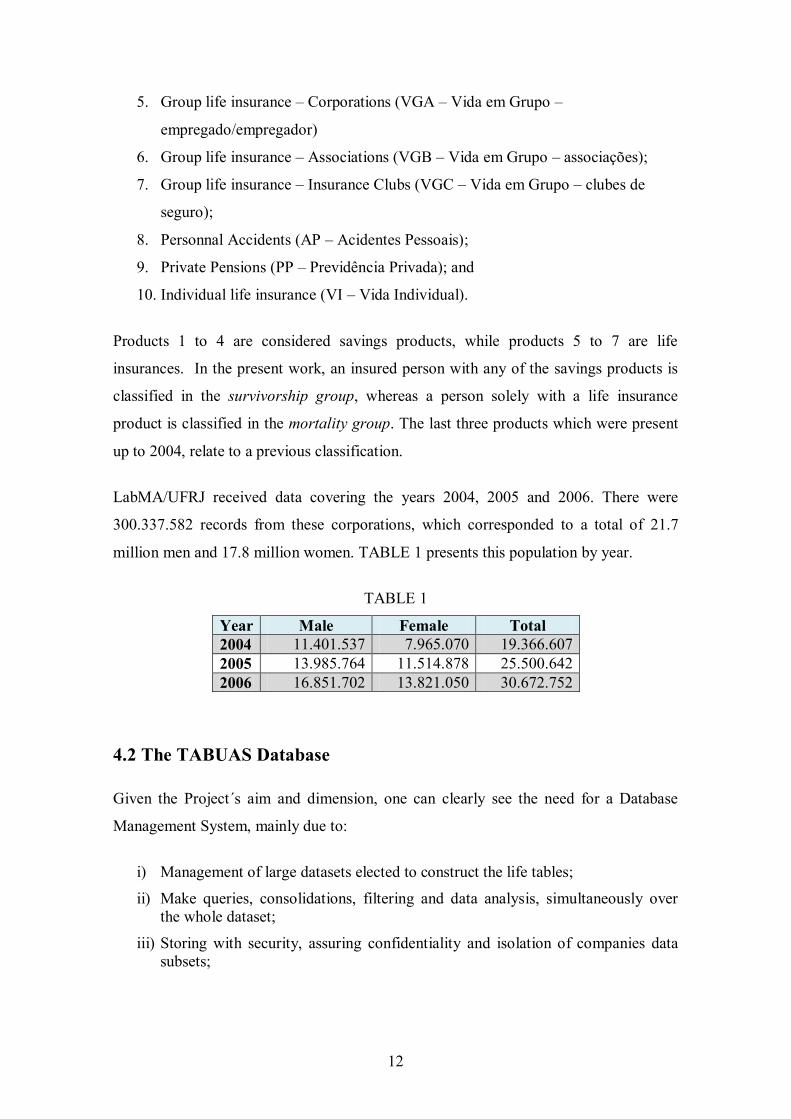
LabMA/UFRJ received data covering the years 2004, 2005 and 2006. There were

300.337.582 records from these corporations, which corresponded to a total of 21.7

million men and 17.8 million women. TABLE 1 presents this population by year.

TABLE 1 Year Male Female Total 2004 11.401.537 7.965.070 19.366.607 2005 13.985.764 11.514.878 25.500.642 2006 16.851.702 13.821.050 30.672.752

4.2 The TABUAS Database

Given the Project´s aim and dimension, one can clearly see the need for a Database

Management System, mainly due to:

i) Management of large datasets elected to construct the life tables;

ii) Make queries, consolidations, filtering and data analysis, simultaneously over the whole dataset;

iii) Storing with security, assuring confidentiality and isolation of companies data subsets;

13

The database developed within the project was named TABUAS. In what follows, a

series of actions for database construction are commented:

i) Data gathering and transformation of data subsets from the several participating insurance companies;

ii) Storage and security procedures, as well as routines to assure confidentiality;

iii) Data Model of the TABUAS database; and iv) Integration routines of several data sources.

Data Gathering and Transformation

Each participating insurance company sent to LabMA/UFRJ its data sets, recorded

according to SUSEP`s protocol. Each data set was individually incorporated into

TABUAS database. LabMA/UFRJ adopted a different database schema for each

insurance company and calendar year due to confidentiality and data isolation. The C

language was used to program some routines to import each company data set into the

corresponding database schema. For all sessions due to security reasons, log files were

kept in order to allow error tracking in the process. The whole process, as conceived, is

robust and replicable.

Storage, Security and Confidentiality Procedures

The life table project had a major requisite of complete confidentiality of the

information received from the insurance companies. To ensure that this requisite is fully

satisfied the TABUAS database environment was set to partition all data access. A

firewall was set to protect the database environment, as well as, the network of

computers used in project development, which deal directly or indirectly with the data.

Every external data access was forbidden while all internal accesses were logged.

Backup procedures were implemented, particularly, with respect to the integration and

data analysis processes.

“Tabuas” Database Schema

The main objectives of the database model conceived for the life table project were to

aid in the statistical processing and to construct a temporal profile for each individual (a

time line in the Lexis Diagram).

14

The “Tabuas” database was logically and physically divided in two levels. The first

level concerns the process of gathering, importing, transforming and integrating data.

The second level is the basis for conducting data analysis required for the construction

of life tables.

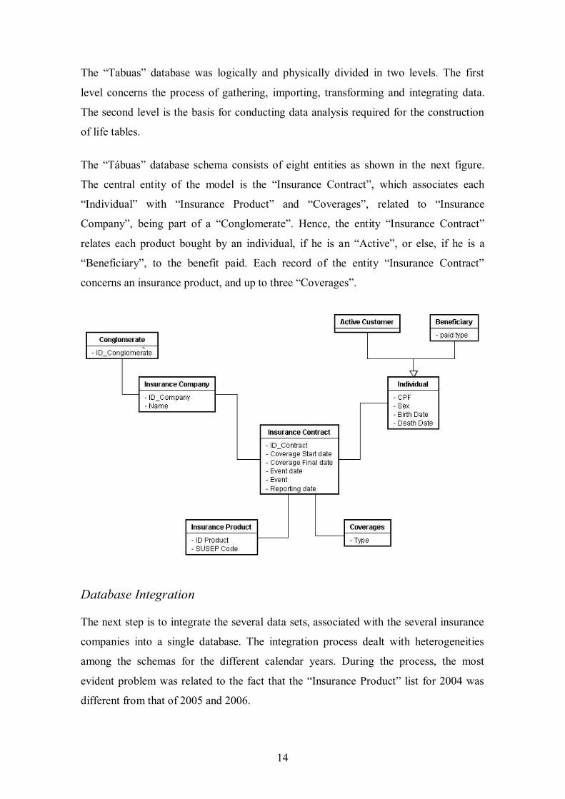
The “Tábuas” database schema consists of eight entities as shown in the next figure.

The central entity of the model is the “Insurance Contract”, which associates each

“Individual” with “Insurance Product” and “Coverages”, related to “Insurance

Company”, being part of a “Conglomerate”. Hence, the entity “Insurance Contract”

relates each product bought by an individual, if he is an “Active”, or else, if he is a

“Beneficiary”, to the benefit paid. Each record of the entity “Insurance Contract”

concerns an insurance product, and up to three “Coverages”.

Database Integration

The next step is to integrate the several data sets, associated with the several insurance

companies into a single database. The integration process dealt with heterogeneities

among the schemas for the different calendar years. During the process, the most

evident problem was related to the fact that the “Insurance Product” list for 2004 was

different from that of 2005 and 2006.

15

The data conversion and integration processes goes through successive steps of filtering

and clustering using database views. To implement the integration of the database as a

whole, 178 database views were programmed. The highest database view hierarchical

level integrates all the data collected from the insurance companies. All data analysis

routines run on this database view.

Data Quality check

In this step a data analysis was performed in order to check the quality of the data

gathered. To do that, three different procedures were implemented:

i) Consistency check of stocks and flows;

ii) CPF – tax registration ID validation check; and

iii) Population and death age and sex distribution check.

This last check was performed for each combination of calendar year, “Insurance

Company”, “Insurance Product” and “Coverage”.

Consistency check of stocks and flows

In the first check performed stocks and flows were verified for consistency: stock at the

begging of the year plus new entries should match stock at the end of the year plus

withdraws.

This Consistency check was performed for the aggregated database by sex and, later on,

tallying by the combination of:

i) Insurance company (23 companies); ii) Calendar year (2004, 2005 and 2006);

iii) Insurance product (defined by SUSEP in 7 categories); iv) Coverage (2 types);

v) Activity status (active or beneficiary); and vi) Age.

16

The second consistency check verified information in adjacent years: stock at the end of

a given calendar year should match the stock at the begging of the following year. This

check was performed for the link between 2004 and 2005, and between 2005 and 2006.

This consist check was also performed for the aggregated database by sex and, later on,

tallying by the same combination described above. These analyses showed some

inconsistencies, which were not particularly important for the project.

Tax Registration ID Validation Check

The validation check of the CPF (tax ID) information was first performed using the

internal consistency check of the tax ID. The CPF consists of a set of 9 digits followed

by 2 control digits. The 2 control digits can be obtained as a function of the previous 9

digits (IRS defines the function). In the validation check, CPFs that did not conform to

the control digit verification were considered invalid and correspond records were

analyzed separately. Afterwards, some combinations that did conform to the control

digit verification but were well known fakes, such as 000.000.001-71, 111.111.111-11,

222.222.222-22, were also considered invalid. In the “Tabuas” database, 13.7% of the

registers contained invalid tax ID numbers, which corresponded to less than 0,1% of the

individuals of the whole database.

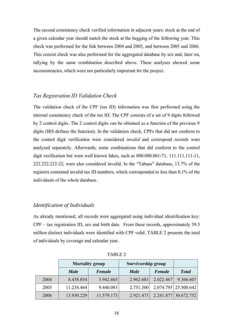
Identification of Individuals

As already mentioned, all records were aggregated using individual identification key:

CPF – tax registration ID, sex and birth date. From these records, approximately 39.5

million distinct individuals were identified with CPF valid. TABLE 2 presents the total

of individuals by coverage and calendar year.

TABLE 2

Mortality group Survivorship group

Male Female Male Female Total

2004 8.438.854 5.942.603 2.962.683 2.022.467 9.366.607

2005 11.234.464 9.440.083 2.751.300 2.074.795 25.500.642

2006 13.930.229 11.579.173 2.921.473 2.241.877 30.672.752

17

CHAPTER 5 – SELECTION OF SUBPOPULATIONS

5.1 Population Distribution and Evolution in Time

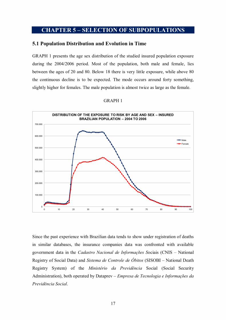
GRAPH 1 presents the age sex distribution of the studied insured population exposure

during the 2004/2006 period. Most of the population, both male and female, lies

between the ages of 20 and 80. Below 18 there is very little exposure, while above 80

the continuous decline is to be expected. The mode occurs around forty something,

slightly higher for females. The male population is almost twice as large as the female.

GRAPH 1

0

100.000

200.000

300.000

400.000

500.000

600.000

700.000

0 10 20 30 40 50 60 70 80 90 100

DISTRIBUTION OF THE EXPOSURE TO RISK BY AGE AND SEX – INSURED BRAZILIAN POPULATION – 2004 TO 2006

Male

Female

Since the past experience with Brazilian data tends to show under registration of deaths

in similar databases, the insurance companies data was confronted with available

government data in the Cadastro Nacional de Informações Sociais (CNIS – National

Registry of Social Data) and Sistema de Controle de Óbitos (SISOBI – National Death

Registry System) of the Ministério da Previdência Social (Social Security

Administration), both operated by Dataprev – Empresa de Tecnologia e Informações da

Previdência Social.

18

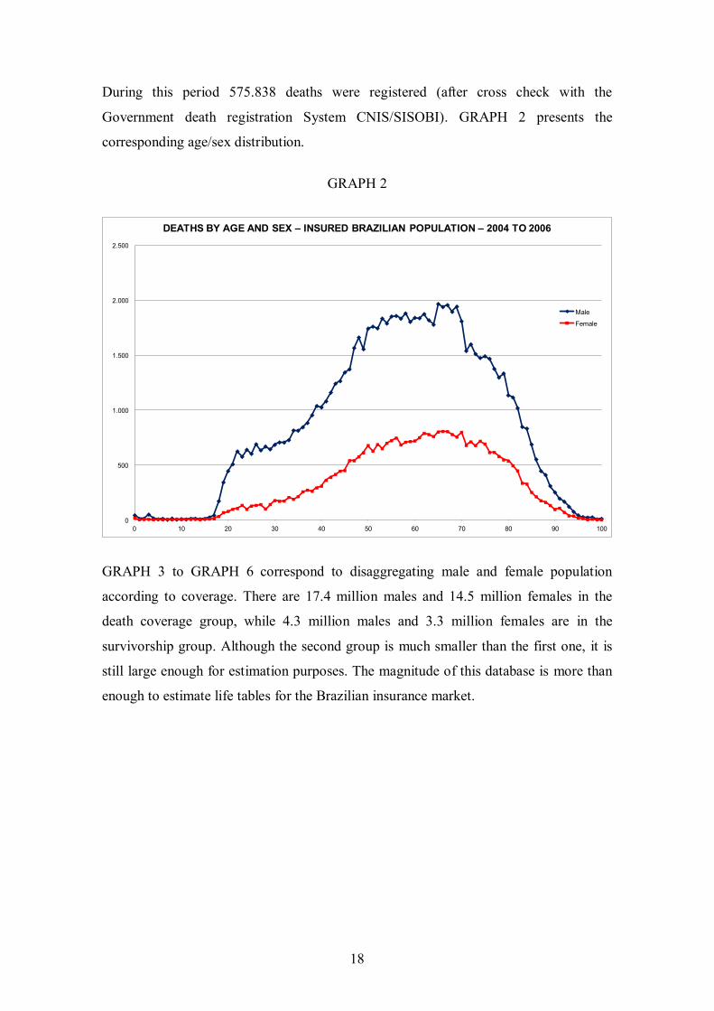
During this period 575.838 deaths were registered (after cross check with the

Government death registration System CNIS/SISOBI). GRAPH 2 presents the

corresponding age/sex distribution.

GRAPH 2

0

500

1.000

1.500

2.000

2.500

0 10 20 30 40 50 60 70 80 90 100

DEATHS BY AGE AND SEX – INSURED BRAZILIAN POPULATION – 2004 TO 2006

Male

Female

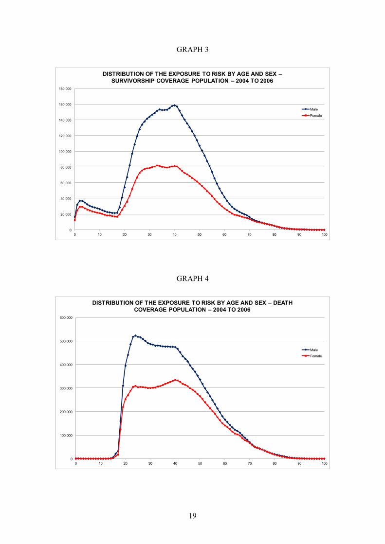
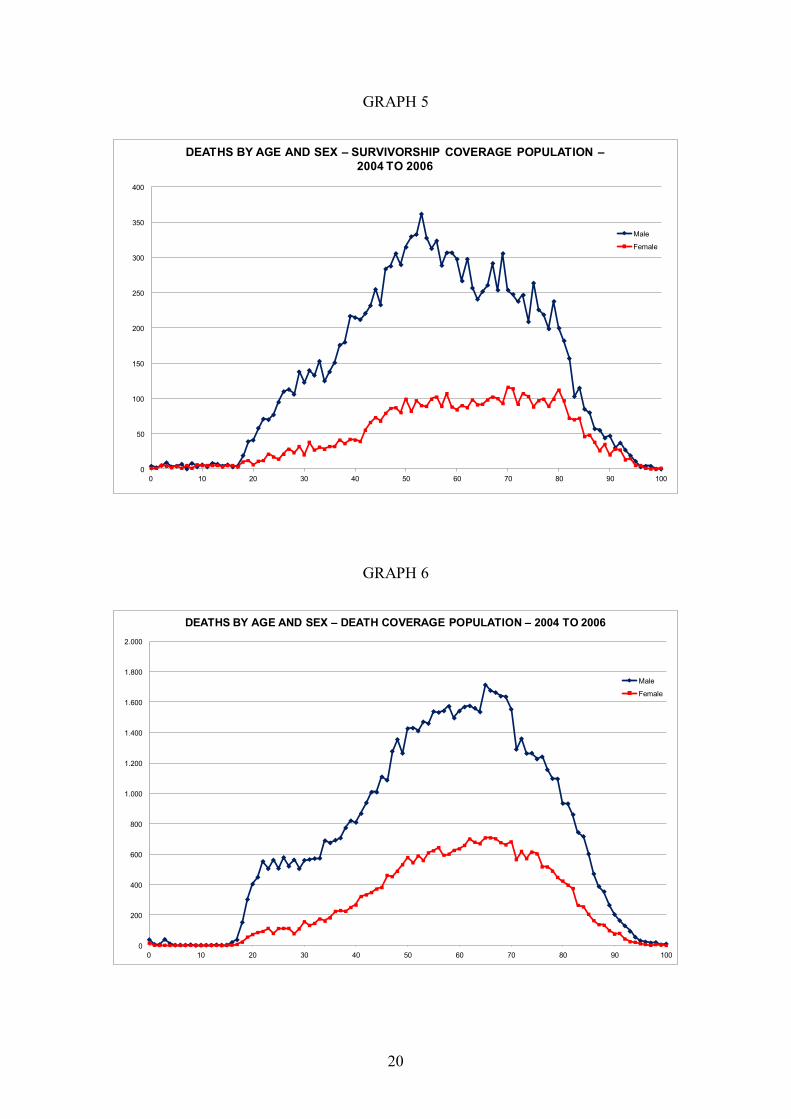
GRAPH 3 to GRAPH 6 correspond to disaggregating male and female population

according to coverage. There are 17.4 million males and 14.5 million females in the

death coverage group, while 4.3 million males and 3.3 million females are in the

survivorship group. Although the second group is much smaller than the first one, it is

still large enough for estimation purposes. The magnitude of this database is more than

enough to estimate life tables for the Brazilian insurance market.

19

GRAPH 3

0

20.000

40.000

60.000

80.000

100.000

120.000

140.000

160.000

180.000

0 10 20 30 40 50 60 70 80 90 100

DISTRIBUTION OF THE EXPOSURE TO RISK BY AGE AND SEX –SURVIVORSHIP COVERAGE POPULATION – 2004 TO 2006

Male

Female

GRAPH 4

0

100.000

200.000

300.000

400.000

500.000

600.000

0 10 20 30 40 50 60 70 80 90 100

DISTRIBUTION OF THE EXPOSURE TO RISK BY AGE AND SEX – DEATH COVERAGE POPULATION – 2004 TO 2006

Male

Female

20

GRAPH 5

0

50

100

150

200

250

300

350

400

0 10 20 30 40 50 60 70 80 90 100

DEATHS BY AGE AND SEX – SURVIVORSHIP COVERAGE POPULATION –2004 TO 2006

Male

Female

GRAPH 6

0

200

400

600

800

1.000

1.200

1.400

1.600

1.800

2.000

0 10 20 30 40 50 60 70 80 90 100

DEATHS BY AGE AND SEX – DEATH COVERAGE POPULATION – 2004 TO 2006

Male

Female

21

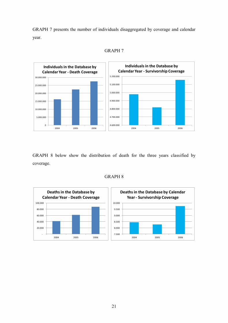
GRAPH 7 presents the number of individuals disaggregated by coverage and calendar

year.

GRAPH 7

0

5.000.000

10.000.000

15.000.000

20.000.000

25.000.000

30.000.000

2004 2005 2006

Individuals in the Database by Calendar Year - Death Coverage

4.600.000

4.700.000

4.800.000

4.900.000

5.000.000

5.100.000

5.200.000

2004 2005 2006

Individuals in the Database by Calendar Year - Survivorship Coverage

GRAPH 8 below show the distribution of death for the three years classified by

coverage.

GRAPH 8

-

20.000

40.000

60.000

80.000

100.000

2004 2005 2006

Deaths in the Database by Calendar Year - Death Coverage

7.500

8.000

8.500

9.000

9.500

10.000

2004 2005 2006

Deaths in the Database by Calendar Year - Survivorship Coverage

22

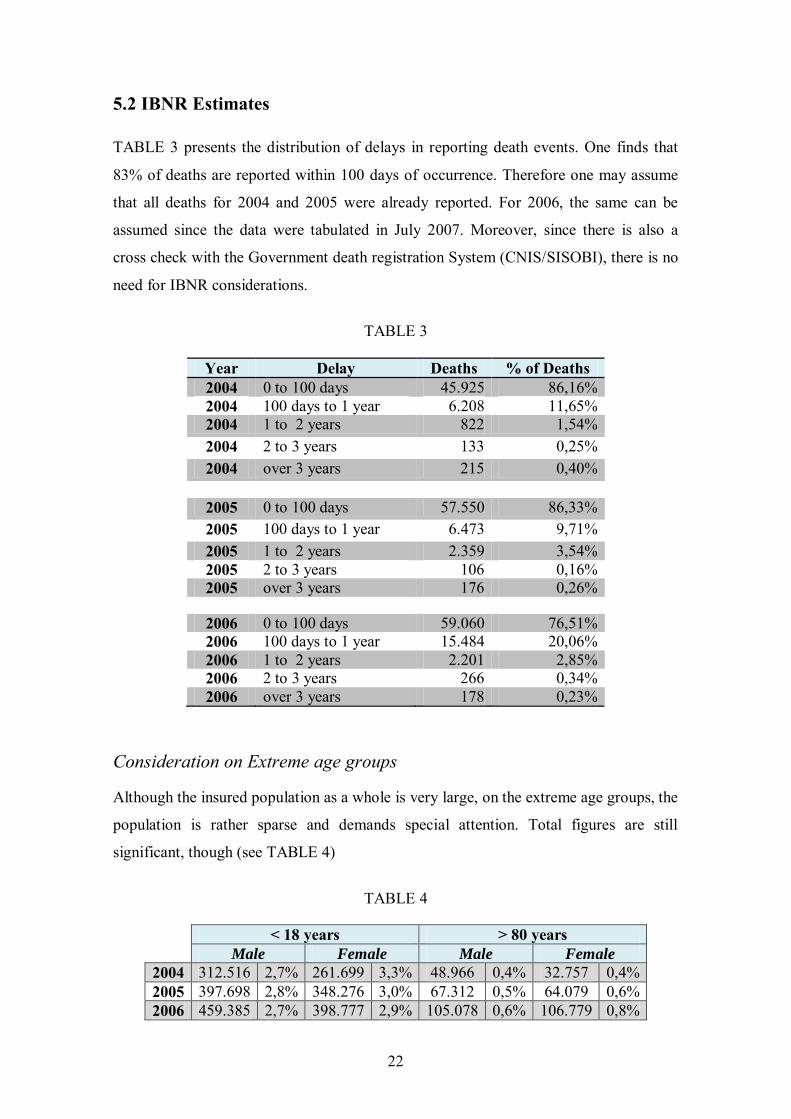
5.2 IBNR Estimates

TABLE 3 presents the distribution of delays in reporting death events. One finds that

83% of deaths are reported within 100 days of occurrence. Therefore one may assume

that all deaths for 2004 and 2005 were already reported. For 2006, the same can be

assumed since the data were tabulated in July 2007. Moreover, since there is also a

cross check with the Government death registration System (CNIS/SISOBI), there is no

need for IBNR considerations.

TABLE 3

Year Delay Deaths % of Deaths 2004 0 to 100 days 45.925 86,16% 2004 100 days to 1 year 6.208 11,65% 2004 1 to 2 years 822 1,54% 2004 2 to 3 years 133 0,25% 2004 over 3 years 215 0,40%

2005 0 to 100 days 57.550 86,33% 2005 100 days to 1 year 6.473 9,71% 2005 1 to 2 years 2.359 3,54% 2005 2 to 3 years 106 0,16% 2005 over 3 years 176 0,26%

2006 0 to 100 days 59.060 76,51% 2006 100 days to 1 year 15.484 20,06% 2006 1 to 2 years 2.201 2,85% 2006 2 to 3 years 266 0,34% 2006 over 3 years 178 0,23%

Consideration on Extreme age groups

Although the insured population as a whole is very large, on the extreme age groups, the

population is rather sparse and demands special attention. Total figures are still

significant, though (see TABLE 4)

TABLE 4

< 18 years > 80 years Male Female Male Female

2004 312.516 2,7% 261.699 3,3% 48.966 0,4% 32.757 0,4% 2005 397.698 2,8% 348.276 3,0% 67.312 0,5% 64.079 0,6% 2006 459.385 2,7% 398.777 2,9% 105.078 0,6% 106.779 0,8%

23

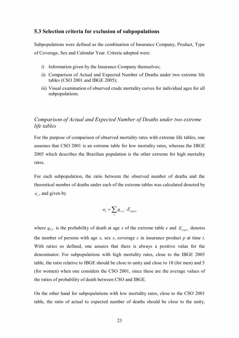
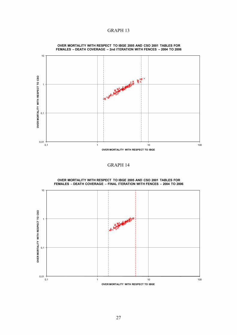
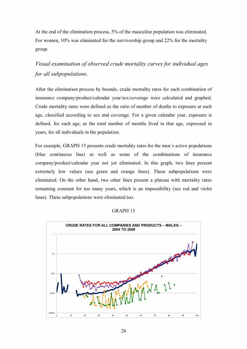
5.3 Selection criteria for exclusion of subpopulations

Subpopulations were defined as the combination of Insurance Company, Product, Type

of Coverage, Sex and Calendar Year. Criteria adopted were:

i) Information given by the Insurance Company themselves;

ii) Comparison of Actual and Expected Number of Deaths under two extreme life tables (CSO 2001 and IBGE 2005);

iii) Visual examination of observed crude mortality curves for individual ages for all subpopulations.

Comparison of Actual and Expected Number of Deaths under two extreme life tables

For the purpose of comparison of observed mortality rates with extreme life tables, one

assumes that CSO 2001 is an extreme table for low mortality rates, whereas the IBGE

2005 which describes the Brazilian population is the other extreme for high mortality

rates.

For each subpopulation, the ratio between the observed number of deaths and the

theoretical number of deaths under each of the extreme tables was calculated denoted by

eo , and given by

xspctx

exe Eqo ,

where qx,e is the probability of death at age x of the extreme table e and xspctE denotes

the number of persons with age x, sex s, coverage c in insurance product p at time t.

With ratios so defined, one assures that there is always a positive value for the

denominator. For subpopulations with high mortality rates, close to the IBGE 2005

table, the ratio relative to IBGE should be close to unity and close to 10 (for men) and 5

(for women) when one considers the CSO 2001, since these are the average values of

the ratios of probability of death between CSO and IBGE.

On the other hand for subpopulations with low mortality rates, close to the CSO 2001

table, the ratio of actual to expected number of deaths should be close to the unity,

24

whereas close to 1/10 (for men) and 1/5 (for women) when the IBGE table is

considered.

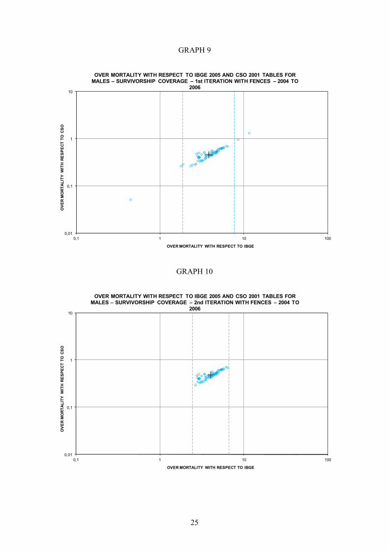
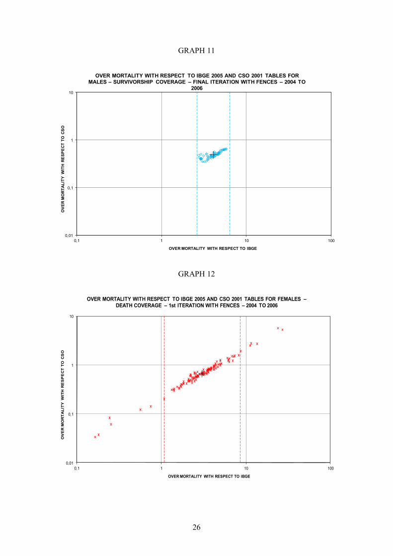
These ratios were plotted in an x-y graph, with the ratio relative to IBGE in the x-axis

and the ratio relative to CSO in the y-axis. One should expect, roughly, in case all

subpopulations were submitted to the same mortality pattern, that all points should be in

a cloud around a center point, close to each other, probably close to a straight line.

Points far away from the central point of the cloud should be discharged, since they

would probably involve data errors and could bias the results.

Since the numerator of each fraction is the actual number of deaths for each

subpopulation, and since the number of deaths, considered as a random variable, is the

sum of independent binomial random variables, one for each age, one may assume that

the numerator of each fraction will be approximately normally distributed. Therefore,

inspired by Tukey (1977), one can calculate bounds that will define subpopulation

outliers. For the present case, all subpopulation outside these bounds were discharged.

The process of establishing bounds and not considering subpopulation outliers was

carried on interactively until no further outliers existed. Each bound was established by

adding and subtracting 1.5 inter quartile distance to the median, thus leaving roughly

95% of the points inside.

The graphs below present over mortality calculated with respect to the IBGE 2005 and

CSO 2001 tables for subpopulations with death and survivorship coverage according to

sex and calendar year. In these graphs, crosses indicate medians and the bounds are

designed as dashed lines. Different colors indicate different years in order to stress

possible time trends. These graphs do not show any temporal evolution in mortality.

25

GRAPH 9

0,01

0,1

1

10

0,1 1 10 100

OVE

R M

ORT

ALIT

Y W

ITH

RESP

ECT

TO C

SO

OVER MORTALITY WITH RESPECT TO IBGE

OVER MORTALITY WITH RESPECT TO IBGE 2005 AND CSO 2001 TABLES FOR MALES – SURVIVORSHIP COVERAGE – 1st ITERATION WITH FENCES – 2004 TO

2006

GRAPH 10

0,01

0,1

1

10

0,1 1 10 100

OVE

R M

ORT

ALIT

Y W

ITH

RESP

ECT

TO C

SO

OVER MORTALITY WITH RESPECT TO IBGE

OVER MORTALITY WITH RESPECT TO IBGE 2005 AND CSO 2001 TABLES FOR MALES – SURVIVORSHIP COVERAGE – 2nd ITERATION WITH FENCES – 2004 TO

2006

26

GRAPH 11

0,01

0,1

1

10

0,1 1 10 100

OVE

R M

ORT

ALIT

Y W

ITH

RESP

ECT

TO C

SO

OVER MORTALITY WITH RESPECT TO IBGE

OVER MORTALITY WITH RESPECT TO IBGE 2005 AND CSO 2001 TABLES FOR MALES – SURVIVORSHIP COVERAGE – FINAL ITERATION WITH FENCES – 2004 TO

2006

GRAPH 12

0,01

0,1

1

10

0,1 1 10 100

OV

ER

MO

RTA

LITY

WIT

H R

ES

PE

CT

TO C

SO

OVER MORTALITY WITH RESPECT TO IBGE

OVER MORTALITY WITH RESPECT TO IBGE 2005 AND CSO 2001 TABLES FOR FEMALES –DEATH COVERAGE – 1st ITERATION WITH FENCES – 2004 TO 2006

27

GRAPH 13

0,01

0,1

1

10

0,1 1 10 100

OVE

R M

ORT

ALIT

Y W

ITH

RESP

ECT

TO C

SO

OVER MORTALITY WITH RESPECT TO IBGE

OVER MORTALITY WITH RESPECT TO IBGE 2005 AND CSO 2001 TABLES FOR FEMALES – DEATH COVERAGE – 2nd ITERATION WITH FENCES – 2004 TO 2006

GRAPH 14

0,01

0,1

1

10

0,1 1 10 100

OVE

R M

ORT

ALIT

Y W

ITH

RESP

ECT

TO C

SO

OVER MORTALITY WITH RESPECT TO IBGE

OVER MORTALITY WITH RESPECT TO IBGE 2005 AND CSO 2001 TABLES FOR FEMALES – DEATH COVERAGE – FINAL ITERATION WITH FENCES – 2004 TO 2006

28

At the end of the elimination process, 5% of the masculine population was eliminated.

For women, 10% was eliminated for the survivorship group and 22% for the mortality

group.

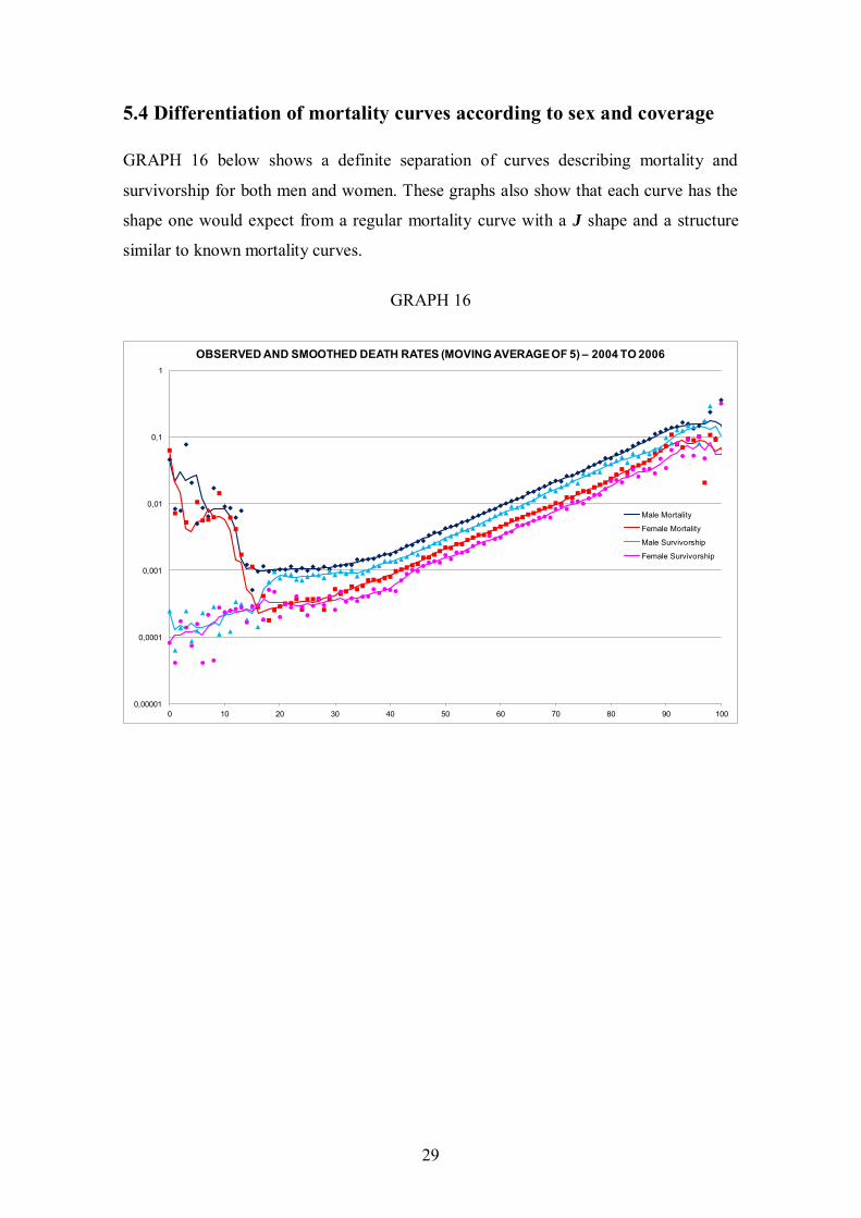
Visual examination of observed crude mortality curves for individual ages

for all subpopulations.

After the elimination process by bounds, crude mortality rates for each combination of

insurance company/product/calendar year/sex/coverage were calculated and graphed.

Crude mortality rates were defined as the ratio of number of deaths to exposure at each

age, classified according to sex and coverage. For a given calendar year, exposure is

defined, for each age, as the total number of months lived in that age, expressed in

years, for all individuals in the population.

For example, GRAPH 15 presents crude mortality rates for the men´s active populations

(blue continuous line) as well as some of the combinations of insurance

company/product/calendar year not yet eliminated. In this graph, two lines present

extremely low values (see green and orange lines). These subpopulations were

eliminated. On the other hand, two other lines present a plateau with mortality rates

remaining constant for too many years, which is an impossibility (see red and violet

lines). These subpopulations were eliminated too.

GRAPH 15

0,0001

0,001

0,01

0,1

1

0 10 20 30 40 50 60 70 80 90 100

CRUDE RATES FOR ALL COMPANIES AND PRODUCTS – MALES –2004 TO 2006

29

5.4 Differentiation of mortality curves according to sex and coverage

GRAPH 16 below shows a definite separation of curves describing mortality and

survivorship for both men and women. These graphs also show that each curve has the

shape one would expect from a regular mortality curve with a J shape and a structure

similar to known mortality curves.

GRAPH 16

0,00001

0,0001

0,001

0,01

0,1

1

0 10 20 30 40 50 60 70 80 90 100

OBSERVED AND SMOOTHED DEATH RATES (MOVING AVERAGE OF 5) – 2004 TO 2006

Male Mortality

Female Mortality

Male Survivorship

Female Survivorship

30

Men

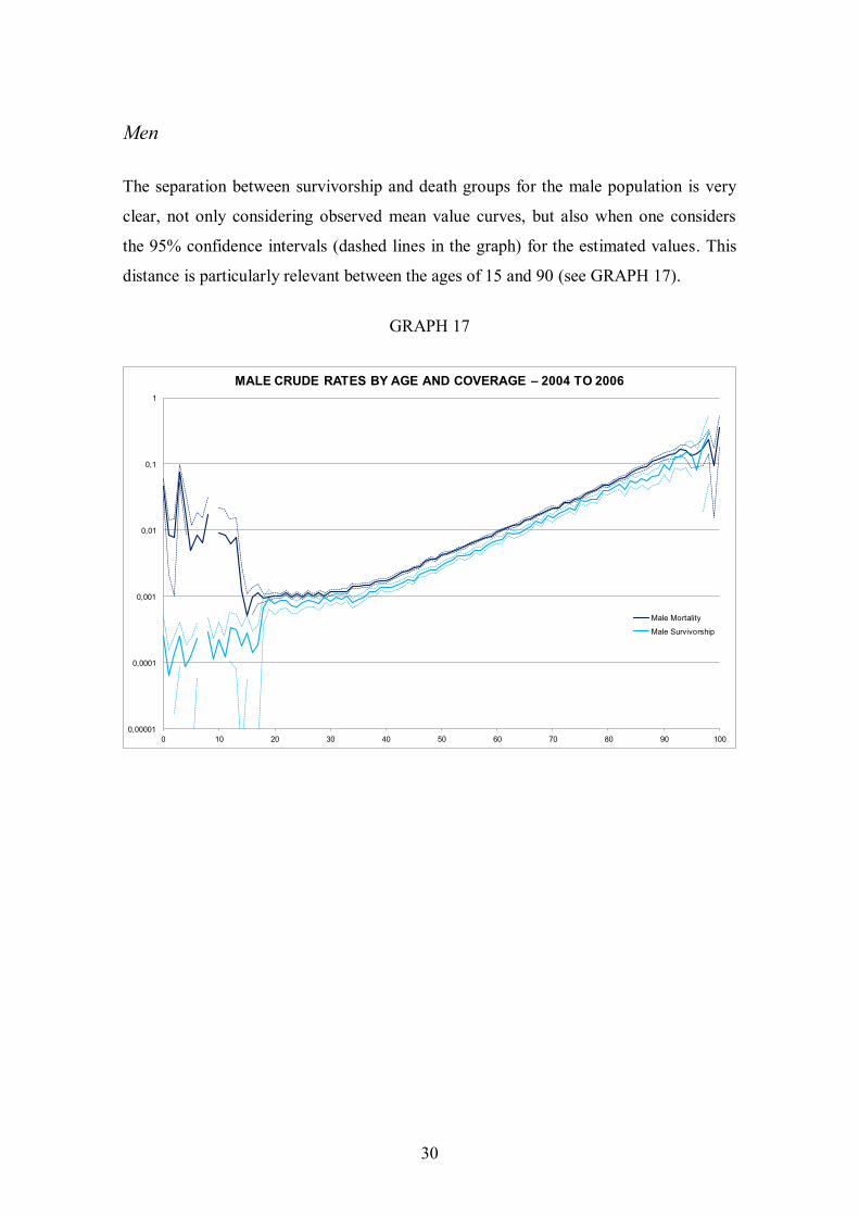
The separation between survivorship and death groups for the male population is very

clear, not only considering observed mean value curves, but also when one considers

the 95% confidence intervals (dashed lines in the graph) for the estimated values. This

distance is particularly relevant between the ages of 15 and 90 (see GRAPH 17).

GRAPH 17

0,00001

0,0001

0,001

0,01

0,1

1

0 10 20 30 40 50 60 70 80 90 100

MALE CRUDE RATES BY AGE AND COVERAGE – 2004 TO 2006

Male Mortality

Male Survivorship

31

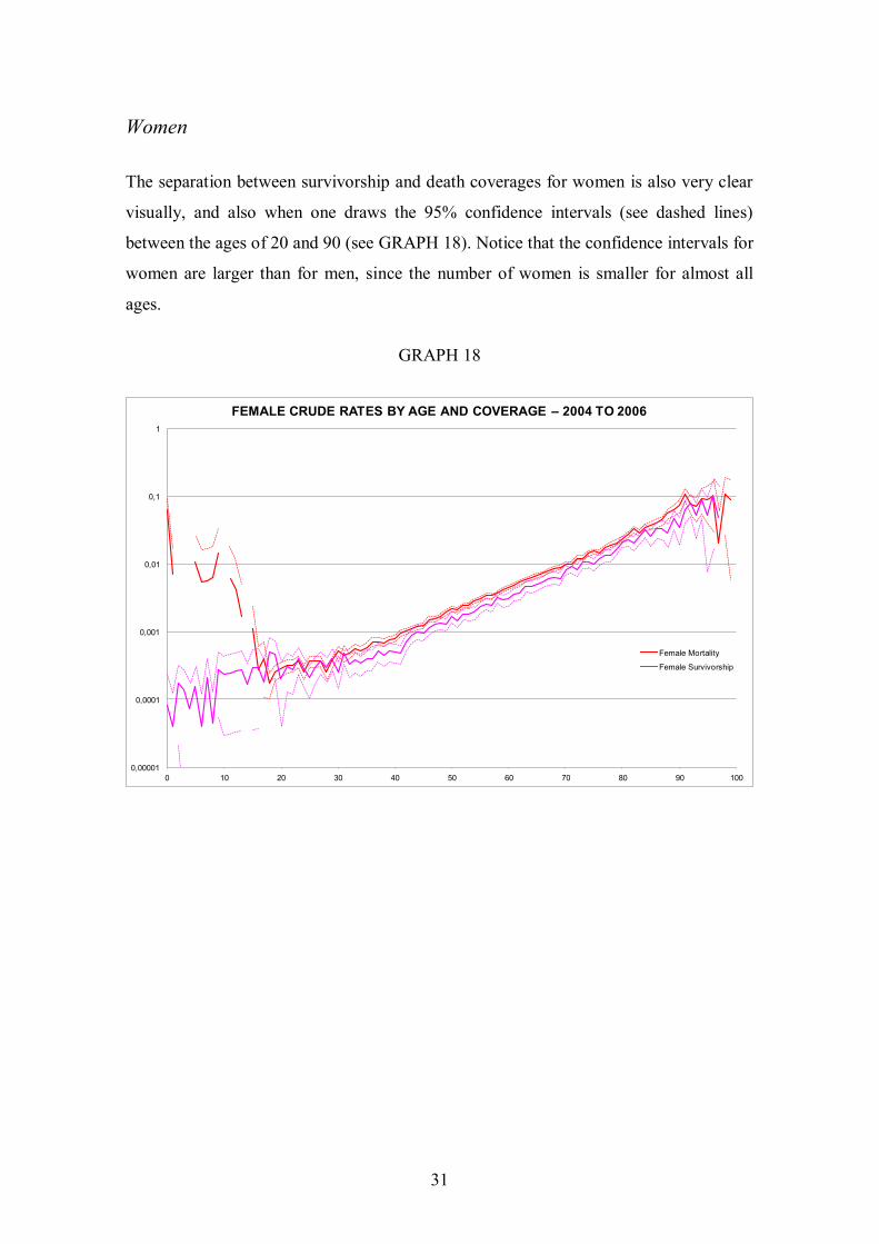
Women

The separation between survivorship and death coverages for women is also very clear

visually, and also when one draws the 95% confidence intervals (see dashed lines)

between the ages of 20 and 90 (see GRAPH 18). Notice that the confidence intervals for

women are larger than for men, since the number of women is smaller for almost all

ages.

GRAPH 18

0,00001

0,0001

0,001

0,01

0,1

1

0 10 20 30 40 50 60 70 80 90 100

FEMALE CRUDE RATES BY AGE AND COVERAGE – 2004 TO 2006

Female Mortality

Female Survivorship

32

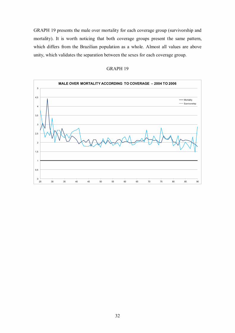
GRAPH 19 presents the male over mortality for each coverage group (survivorship and

mortality). It is worth noticing that both coverage groups present the same pattern,

which differs from the Brazilian population as a whole. Almost all values are above

unity, which validates the separation between the sexes for each coverage group.

GRAPH 19

0

0,5

1

1,5

2

2,5

3

3,5

4

4,5

5

25 30 35 40 45 50 55 60 65 70 75 80 85 90

MALE OVER MORTALITY ACCORDING TO COVERAGE – 2004 TO 2006

Mortality

Survivorship

33

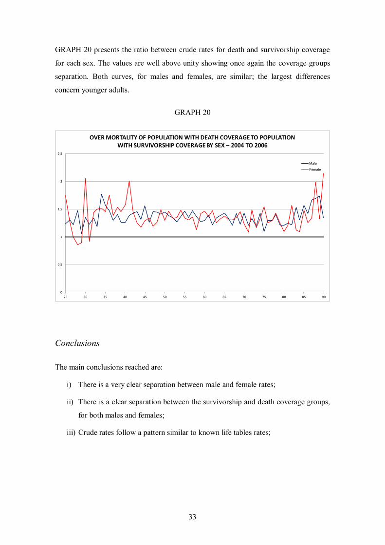
GRAPH 20 presents the ratio between crude rates for death and survivorship coverage

for each sex. The values are well above unity showing once again the coverage groups

separation. Both curves, for males and females, are similar; the largest differences

concern younger adults.

GRAPH 20

0

0,5

1

1,5

2

2,5

25 30 35 40 45 50 55 60 65 70 75 80 85 90

OVER MORTALITY OF POPULATION WITH DEATH COVERAGE TO POPULATION WITH SURVIVORSHIP COVERAGE BY SEX – 2004 TO 2006

Male

Female

Conclusions

The main conclusions reached are:

i) There is a very clear separation between male and female rates;

ii) There is a clear separation between the survivorship and death coverage groups,

for both males and females;

iii) Crude rates follow a pattern similar to known life tables rates;

34

CHAPTER 6 – CONSTRUCTION OF LIFE AND SURVIVAL TABLES

6.1. HELIGMAN & POLLARD Model

The model proposed by Heligman & Pollard (1980) has three components: child

mortality, a “hump” for young adult mortality and a component for middle and old ages

mortality:

)1(

2)ln(ln)()( xKGH

xGHFxEDeCBxAxq

.

The Heligman & Pollard model can be viewed as a combination of different parametric

models for describing human mortality. The second component is particularly useful for

describing the mortality of young adults by external causes, a phenomenon which has

been increasing since the middle of last century.

Since the model has nine parameters for the three components, it is very flexible and

can approximate almost all known human mortality experiences. For these reasons, the

Heligman & Pollard model was chosen for construction of mortality and survival tables.

GRAPH 21 shows the three components and the resultant for a typical case.

GRAPH 21

1E-05

0,0001

0,001

0,01

0,1

1

0 5 10 15 20 25 30 35 40 45 50 55 60 65 70 75 80 85 90 95 100

HELIGMAN & POLLARD MODEL COMPONENTS

EARLY CHILDHOOD YOUNG ADULTS SENESCENCE TOTAL

35

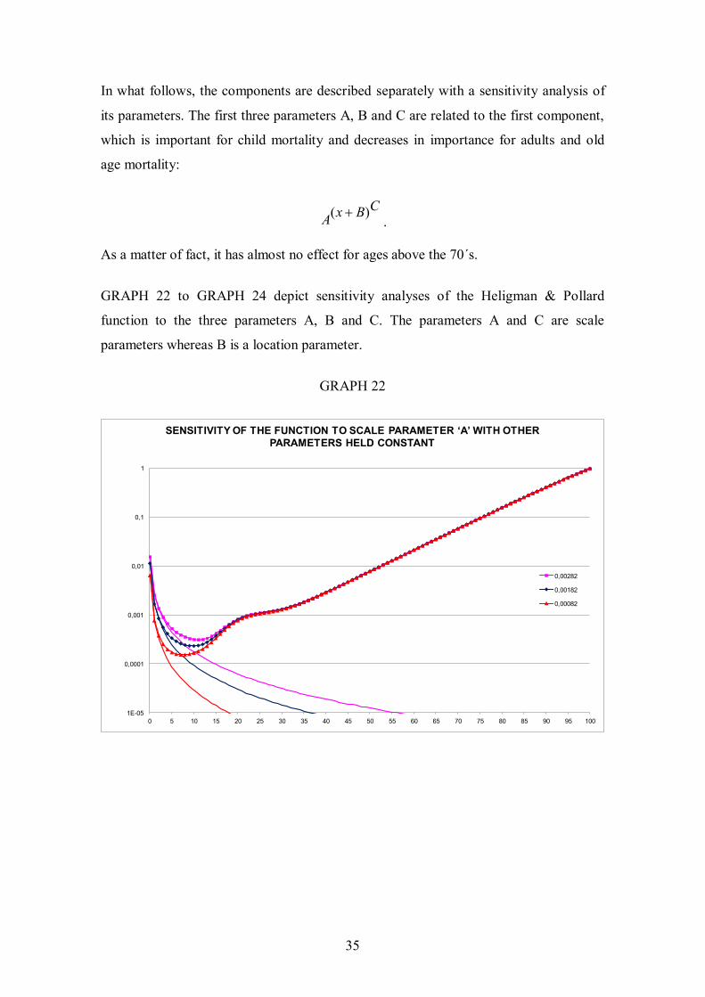
In what follows, the components are described separately with a sensitivity analysis of

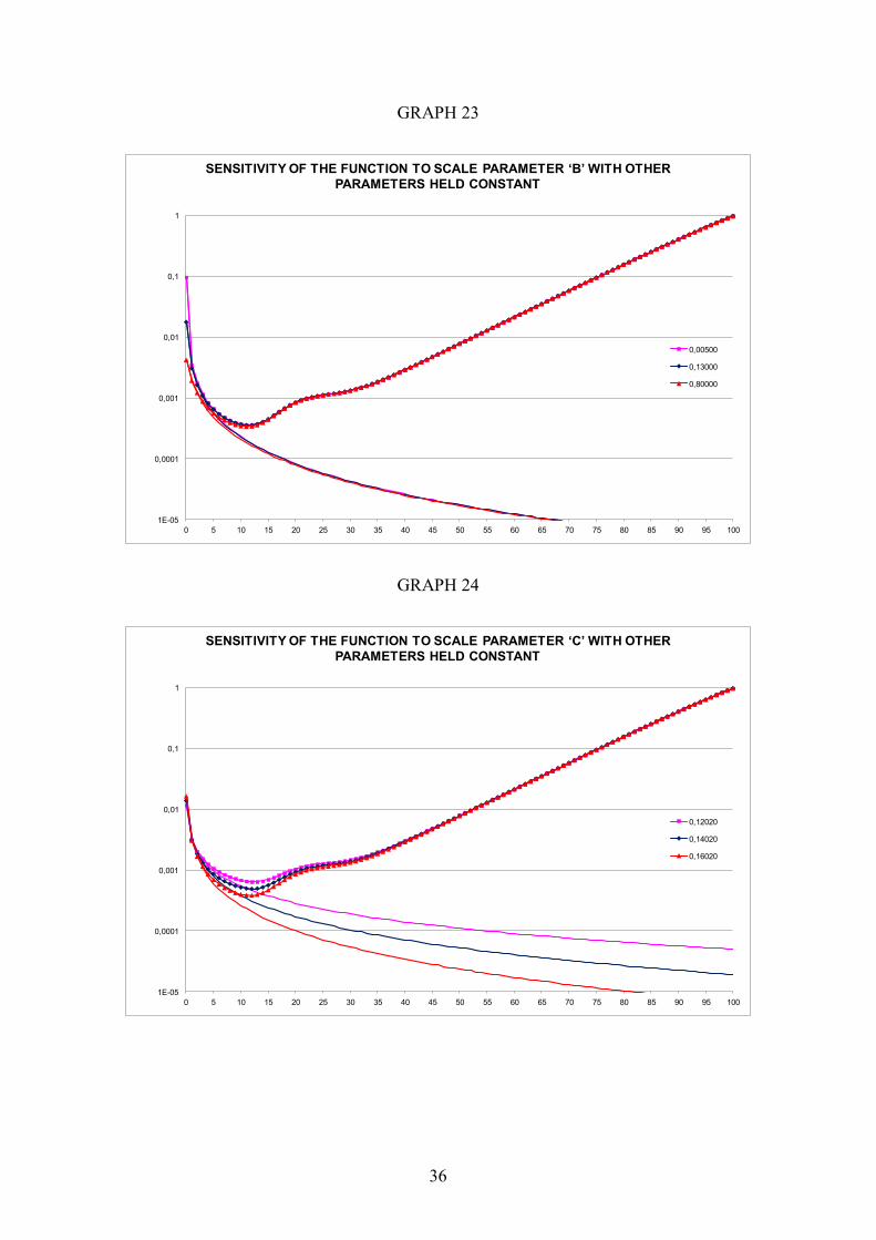
its parameters. The first three parameters A, B and C are related to the first component,

which is important for child mortality and decreases in importance for adults and old

age mortality:

CBxA )( .

As a matter of fact, it has almost no effect for ages above the 70´s.

GRAPH 22 to GRAPH 24 depict sensitivity analyses of the Heligman & Pollard

function to the three parameters A, B and C. The parameters A and C are scale

parameters whereas B is a location parameter.

GRAPH 22

1E-05

0,0001

0,001

0,01

0,1

1

0 5 10 15 20 25 30 35 40 45 50 55 60 65 70 75 80 85 90 95 100

SENSITIVITY OF THE FUNCTION TO SCALE PARAMETER ‘A’ WITH OTHER PARAMETERS HELD CONSTANT

0,00282

0,00182

0,00082

36

GRAPH 23

1E-05

0,0001

0,001

0,01

0,1

1

0 5 10 15 20 25 30 35 40 45 50 55 60 65 70 75 80 85 90 95 100

SENSITIVITY OF THE FUNCTION TO SCALE PARAMETER ‘B’ WITH OTHER PARAMETERS HELD CONSTANT

0,00500

0,13000

0,80000

GRAPH 24

1E-05

0,0001

0,001

0,01

0,1

1

0 5 10 15 20 25 30 35 40 45 50 55 60 65 70 75 80 85 90 95 100

SENSITIVITY OF THE FUNCTION TO SCALE PARAMETER ‘C’ WITH OTHER PARAMETERS HELD CONSTANT

0,12020

0,14020

0,16020

37

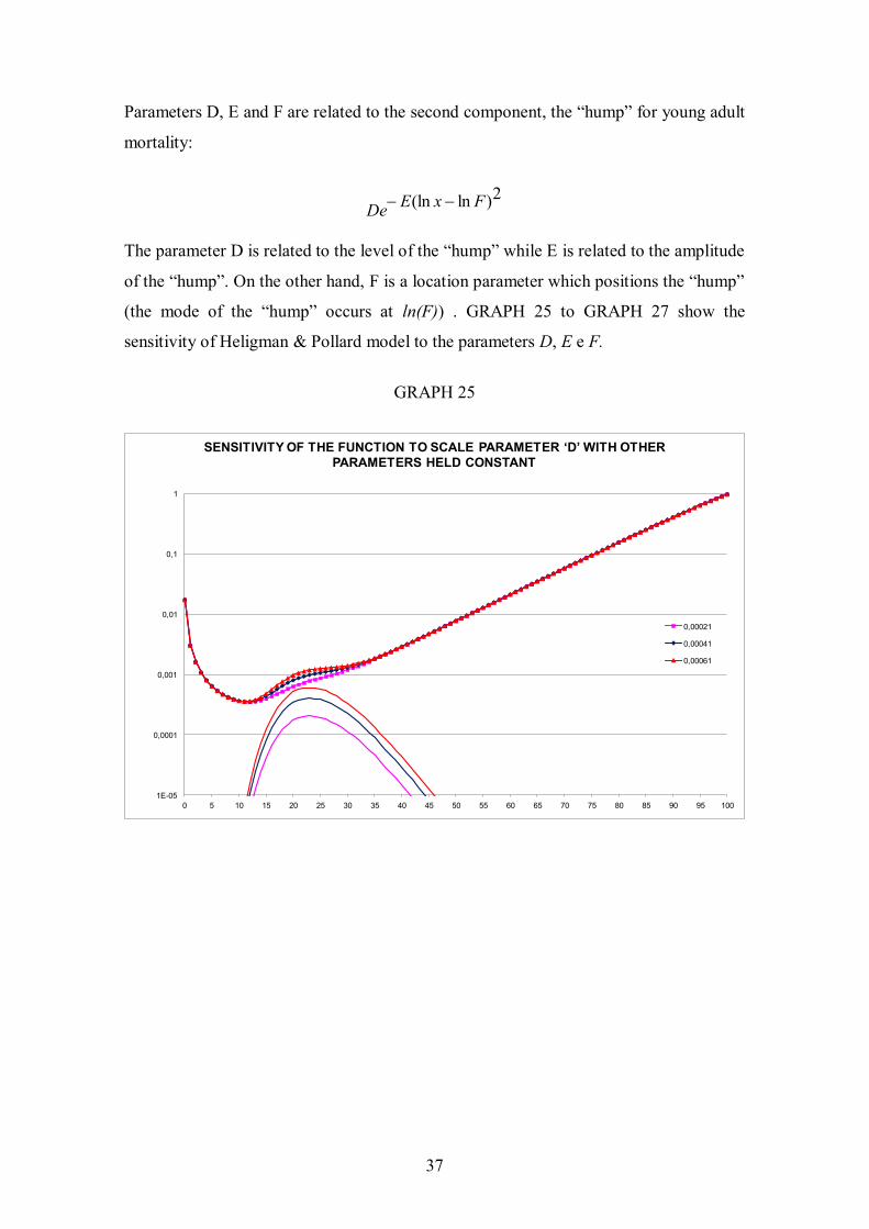
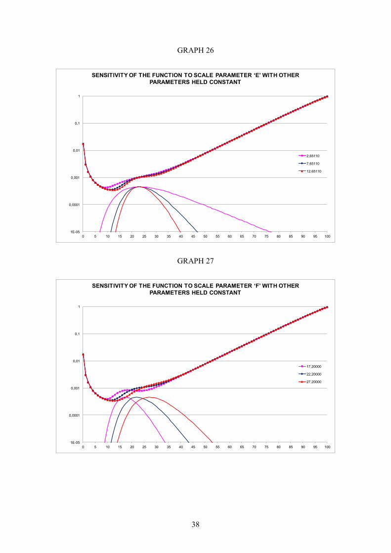
Parameters D, E and F are related to the second component, the “hump” for young adult

mortality:

2)ln(ln FxEDe

The parameter D is related to the level of the “hump” while E is related to the amplitude

of the “hump”. On the other hand, F is a location parameter which positions the “hump”

(the mode of the “hump” occurs at ln(F)) . GRAPH 25 to GRAPH 27 show the

sensitivity of Heligman & Pollard model to the parameters D, E e F.

GRAPH 25

1E-05

0,0001

0,001

0,01

0,1

1

0 5 10 15 20 25 30 35 40 45 50 55 60 65 70 75 80 85 90 95 100

SENSITIVITY OF THE FUNCTION TO SCALE PARAMETER ‘D’ WITH OTHER PARAMETERS HELD CONSTANT

0,00021

0,00041

0,00061

38

GRAPH 26

1E-05

0,0001

0,001

0,01

0,1

1

0 5 10 15 20 25 30 35 40 45 50 55 60 65 70 75 80 85 90 95 100

SENSITIVITY OF THE FUNCTION TO SCALE PARAMETER ‘E’ WITH OTHER PARAMETERS HELD CONSTANT

2,65110

7,65110

12,65110

GRAPH 27

1E-05

0,0001

0,001

0,01

0,1

1

0 5 10 15 20 25 30 35 40 45 50 55 60 65 70 75 80 85 90 95 100

SENSITIVITY OF THE FUNCTION TO SCALE PARAMETER ‘F’ WITH OTHER PARAMETERS HELD CONSTANT

17,20000

22,20000

27,20000

39

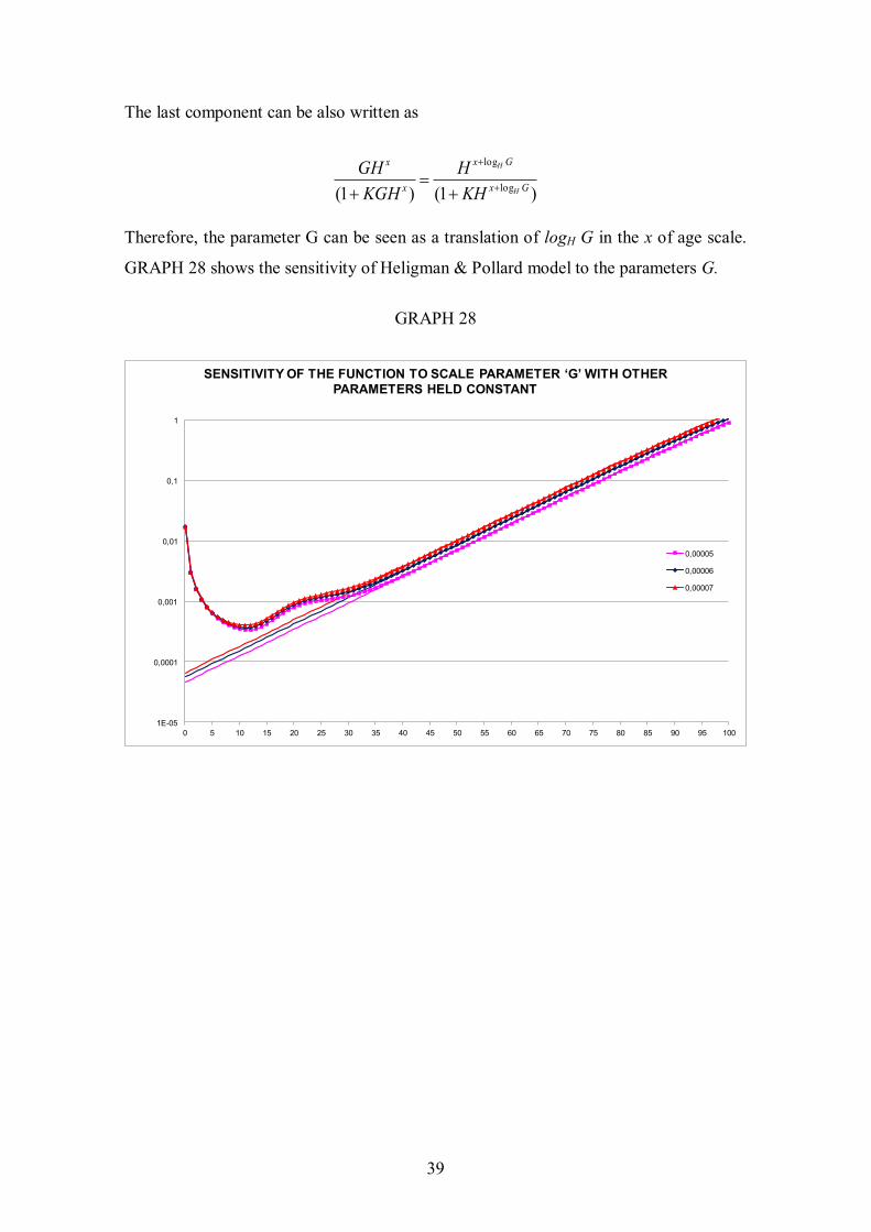
The last component can be also written as

)1()1( log

log

Gx

Gx

x

x

H

H

KHH

KGHGH

Therefore, the parameter G can be seen as a translation of logH G in the x of age scale.

GRAPH 28 shows the sensitivity of Heligman & Pollard model to the parameters G.

GRAPH 28

1E-05

0,0001

0,001

0,01

0,1

1

0 5 10 15 20 25 30 35 40 45 50 55 60 65 70 75 80 85 90 95 100

SENSITIVITY OF THE FUNCTION TO SCALE PARAMETER ‘G’ WITH OTHER PARAMETERS HELD CONSTANT

0,00005

0,00006

0,00007

40

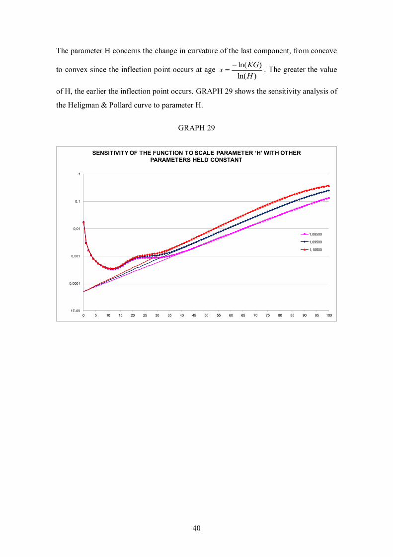
The parameter H concerns the change in curvature of the last component, from concave

to convex since the inflection point occurs at age )ln(

)ln(HKGx

. The greater the value

of H, the earlier the inflection point occurs. GRAPH 29 shows the sensitivity analysis of

the Heligman & Pollard curve to parameter H.

GRAPH 29

1E-05

0,0001

0,001

0,01

0,1

1

0 5 10 15 20 25 30 35 40 45 50 55 60 65 70 75 80 85 90 95 100

SENSITIVITY OF THE FUNCTION TO SCALE PARAMETER ‘H’ WITH OTHER PARAMETERS HELD CONSTANT

1,08500

1,09500

1,10500

41

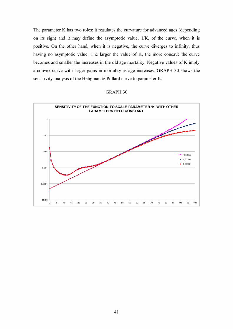
The parameter K has two roles: it regulates the curvature for advanced ages (depending

on its sign) and it may define the asymptotic value, 1/K, of the curve, when it is

positive. On the other hand, when it is negative, the curve diverges to infinity, thus

having no asymptotic value. The larger the value of K, the more concave the curve

becomes and smaller the increases in the old age mortality. Negative values of K imply

a convex curve with larger gains in mortality as age increases. GRAPH 30 shows the

sensitivity analysis of the Heligman & Pollard curve to parameter K.

GRAPH 30

1E-05

0,0001

0,001

0,01

0,1

1

0 5 10 15 20 25 30 35 40 45 50 55 60 65 70 75 80 85 90 95 100

SENSITIVITY OF THE FUNCTION TO SCALE PARAMETER ‘K’ WITH OTHER PARAMETERS HELD CONSTANT

-0,50000

1,00000

4,00000

42

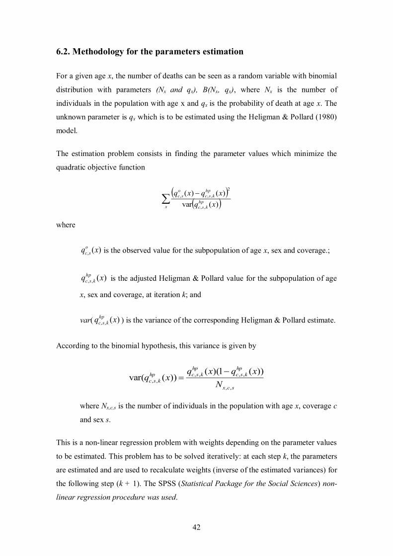
6.2. Methodology for the parameters estimation

For a given age x, the number of deaths can be seen as a random variable with binomial

distribution with parameters (Nx and qx), B(Nx, qx), where Nx is the number of

individuals in the population with age x and qx is the probability of death at age x. The

unknown parameter is qx which is to be estimated using the Heligman & Pollard (1980)

model.

The estimation problem consists in finding the parameter values which minimize the

quadratic objective function

xhp

ksc

hpksc

osc

xqxqxq

)(var)()(

,,

2,,,

where

)(, xqosc is the observed value for the subpopulation of age x, sex and coverage.;

)(,, xqhpksc is the adjusted Heligman & Pollard value for the subpopulation of age

x, sex and coverage, at iteration k; and

var( )(,, xqhpksc ) is the variance of the corresponding Heligman & Pollard estimate.

According to the binomial hypothesis, this variance is given by

scx

hpksc

hpkschp

ksc Nxqxq

xq,,

,,,,,,

))(1)(())(var(

where Nx,c,s is the number of individuals in the population with age x, coverage c

and sex s.

This is a non-linear regression problem with weights depending on the parameter values

to be estimated. This problem has to be solved iteratively: at each step k, the parameters

are estimated and are used to recalculate weights (inverse of the estimated variances) for

the following step (k + 1). The SPSS (Statistical Package for the Social Sciences) non-

linear regression procedure was used.

43

This process resembles the methodology of Generalized Linear Models (see Dobson,

1983 or MacCullagh & Nelder, 1983), except that in GLM the usual packages do it

internally while in this case the weights of each step have to be fed manually. One could

wonder whether using the Poisson or the Normal approximations would lead to a

simplified process. But this is not true since both distributions have age dependent

variances heteroscedasticity, which would not allow a closed solution.

6.3. Curve fitting

The fitting process was conducted in two stages for each sex.

In the first stage, the fitting was conducted, separately for men and women, for the

population independently of the coverage type (survivorship and death). For both sexes,

the adjusted curves presented the three Heligman & Pollard components. It was decided

to estimate the first two Heligman & Pollard components up to the age of 35 years,

independently of the last components. The third component was estimated afterwards,

taking the first two estimated components as given. For this third component the

minimization process was conducted for all ages up to 100 years. It should be noted that

the estimation of the third component parameters is quite independent of the first two

components.

Estimated infant mortality is higher for men but with a declining difference up to 12

years of age. The second component (associated with external causes) starts to appear at

younger ages for women, although it is less pronounced and shows a shorter amplitude

as compared to men. For the country as a whole, this second component is less

pronounced for women, but starts showing up at a later age as compared to men.

44

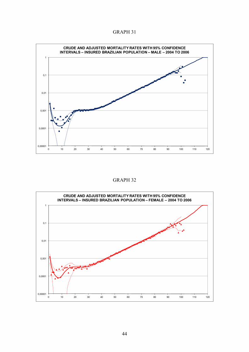
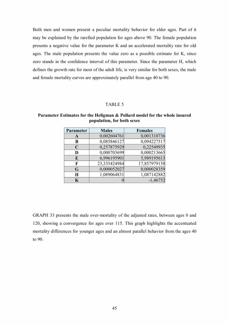
GRAPH 31

0,00001

0,0001

0,001

0,01

0,1

1

0 10 20 30 40 50 60 70 80 90 100 110 120

CRUDE AND ADJUSTED MORTALITY RATES WITH 95% CONFIDENCE INTERVALS – INSURED BRAZILIAN POPULATION – MALE – 2004 TO 2006

GRAPH 32

0,00001

0,0001

0,001

0,01

0,1

1

0 10 20 30 40 50 60 70 80 90 100 110 120

CRUDE AND ADJUSTED MORTALITY RATES WITH 95% CONFIDENCE INTERVALS – INSURED BRAZILIAN POPULATION – FEMALE – 2004 TO 2006

45

Both men and women present a peculiar mortality behavior for elder ages. Part of it

may be explained by the rarefied population for ages above 90. The female population

presents a negative value for the parameter K and an accelerated mortality rate for old

ages. The male population presents the value zero as a possible estimate for K, since

zero stands in the confidence interval of this parameter. Since the parameter H, which

defines the growth rate for most of the adult life, is very similar for both sexes, the male

and female mortality curves are approximately parallel from age 40 to 90.

TABLE 5

Parameter Estimates for the Heligman & Pollard model for the whole insured population, for both sexes

Parameter Males Females

A 0,002604761 0,001310736 B 0,085846127 0,094227517 C 0,257875929 0,22549935 D 0,000703699 0,000213665 E 6,996195901 5,989195613 F 23,335424984 17,857979158 G 0,000052027 0,000028359 H 1,089064831 1,087142882 K 0 -1,46752

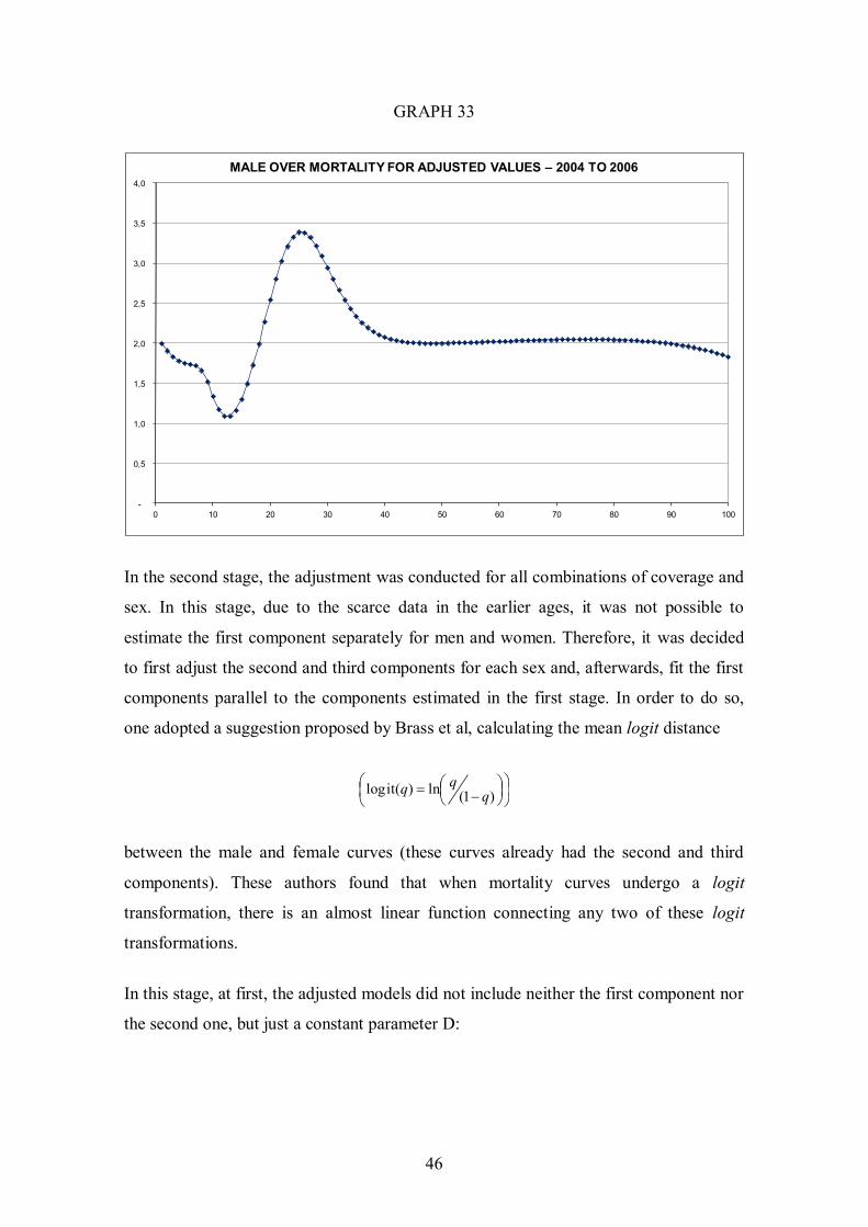
GRAPH 33 presents the male over-mortality of the adjusted rates, between ages 0 and

120, showing a convergence for ages over 115. This graph highlights the accentuated

mortality differences for younger ages and an almost parallel behavior from the ages 40

to 90.

46

GRAPH 33

-

0,5

1,0

1,5

2,0

2,5

3,0

3,5

4,0

0 10 20 30 40 50 60 70 80 90 100

MALE OVER MORTALITY FOR ADJUSTED VALUES – 2004 TO 2006

In the second stage, the adjustment was conducted for all combinations of coverage and

sex. In this stage, due to the scarce data in the earlier ages, it was not possible to

estimate the first component separately for men and women. Therefore, it was decided

to first adjust the second and third components for each sex and, afterwards, fit the first

components parallel to the components estimated in the first stage. In order to do so,

one adopted a suggestion proposed by Brass et al, calculating the mean logit distance

)1(ln)(itlog qqq

between the male and female curves (these curves already had the second and third

components). These authors found that when mortality curves undergo a logit

transformation, there is an almost linear function connecting any two of these logit

transformations.

In this stage, at first, the adjusted models did not include neither the first component nor

the second one, but just a constant parameter D:

47

)1()(,, xKGH

xGHDxqhpksc

.

This model fitting was conducted for ages in the interval between 20 to 100 years. It is

worth noticing that for ages below and above this interval were not considered in the

adjustment process but were incorporated afterwards by an analysis of the adherence of

the estimated curves to the data, taking into consideration confidence intervals for the

death rates.

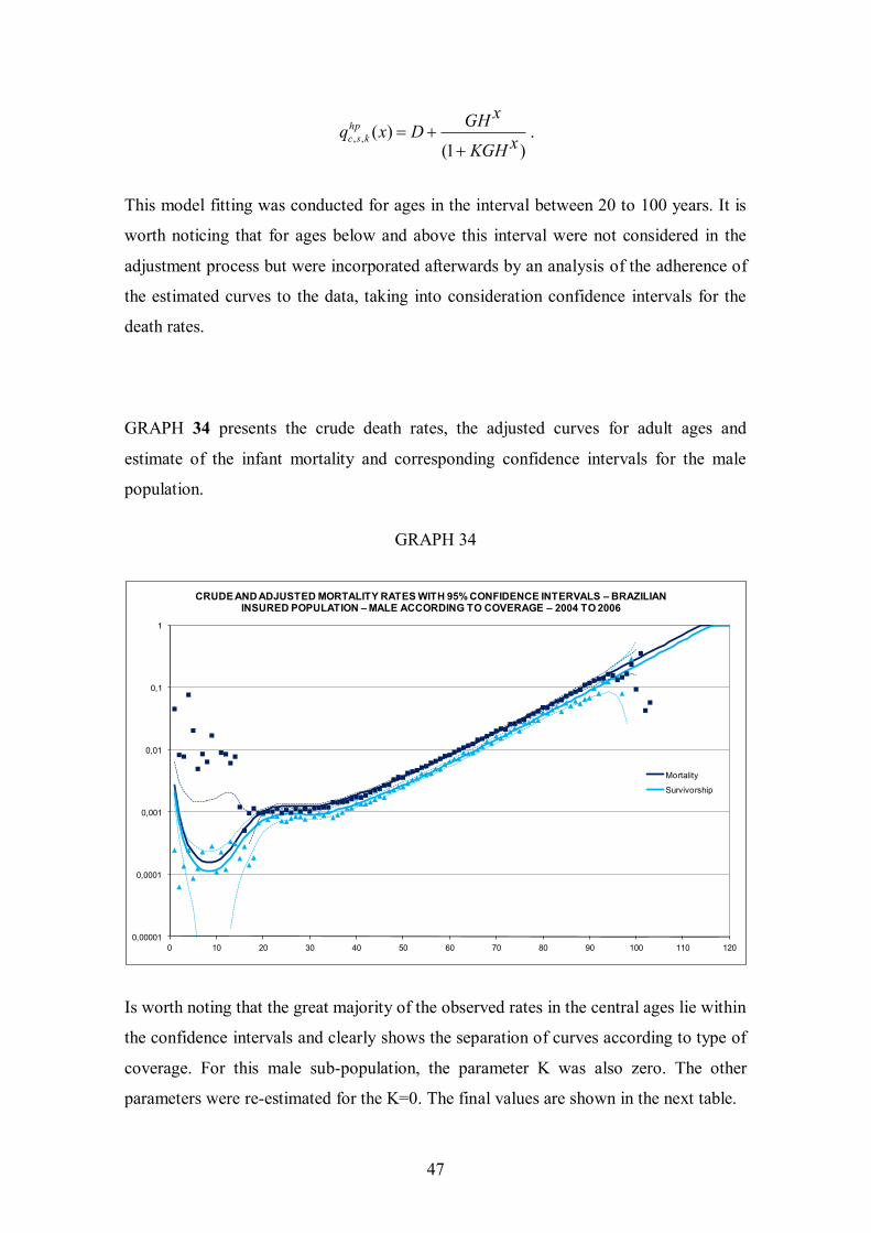
GRAPH 34 presents the crude death rates, the adjusted curves for adult ages and

estimate of the infant mortality and corresponding confidence intervals for the male

population.

GRAPH 34

0,00001

0,0001

0,001

0,01

0,1

1

0 10 20 30 40 50 60 70 80 90 100 110 120

CRUDE AND ADJUSTED MORTALITY RATES WITH 95% CONFIDENCE INTERVALS – BRAZILIAN INSURED POPULATION – MALE ACCORDING TO COVERAGE – 2004 TO 2006

Mortality

Survivorship

Is worth noting that the great majority of the observed rates in the central ages lie within

the confidence intervals and clearly shows the separation of curves according to type of

coverage. For this male sub-population, the parameter K was also zero. The other

parameters were re-estimated for the K=0. The final values are shown in the next table.

48

TABLE 6

Estimates of Heligman & Pollard parameters for the simplified model according to sex and coverage type

Males Females

Survivorship Death Survivorship Death

D 0,00048519 0,00064511 0,00013377 0,000113 G 2,3647E-05 3,5241E-05 1,5425E-05 2,53E-05 H 1,09690236 1,09510716 1,09246271 1,089157 K 0 0 -1,46752 -1,46752

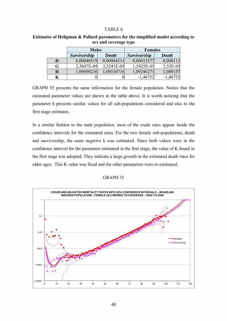
GRAPH 35 presents the same information for the female population. Notice that the

estimated parameter values are shown in the table above. It is worth noticing that the

parameter h presents similar values for all sub-populations considered and also to the

first stage estimates.

In a similar fashion to the male population, most of the crude rates appear inside the

confidence intervals for the estimated rates. For the two female sub-populations, death

and survivorship, the same negative k was estimated. Since both values were in the

confidence interval for the parameter estimated in the first stage, the value of K found in

the first stage was adopted. They indicate a large growth in the estimated death rates for

older ages. This K value was fixed and the other parameters were re-estimated.

GRAPH 35

0,00001

0,0001

0,001

0,01

0,1

1

0 10 20 30 40 50 60 70 80 90 100 110 120

CRUDE AND ADJUSTED MORTALITY RATES WITH 95% CONFIDENCE INTERVALS – BRAZILIAN INSURED POPULATION – FEMALE ACCORDING TO COVERAGE – 2004 TO 2006

Mortality

Survivorship

49

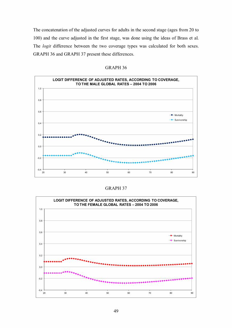
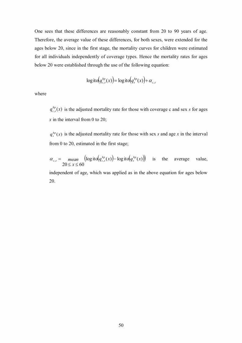
The concatenation of the adjusted curves for adults in the second stage (ages from 20 to

100) and the curve adjusted in the first stage, was done using the ideas of Brass et al.

The logit difference between the two coverage types was calculated for both sexes.

GRAPH 36 and GRAPH 37 present these differences.

GRAPH 36

-0,4

-0,2

0,0

0,2

0,4

0,6

0,8

1,0

20 30 40 50 60 70 80 90

LOGIT DIFFERENCE OF ADJUSTED RATES, ACCORDING TO COVERAGE, TO THE MALE GLOBAL RATES – 2004 TO 2006

Mortality

Survivorship

GRAPH 37

-0,4

-0,2

0,0

0,2

0,4

0,6

0,8

1,0

20 30 40 50 60 70 80 90

LOGIT DIFFERENCE OF ADJUSTED RATES, ACCORDING TO COVERAGE, TO THE FEMALE GLOBAL RATES – 2004 TO 2006

Mortality

Survivorship

50

One sees that these differences are reasonably constant from 20 to 90 years of age.

Therefore, the average value of these differences, for both sexes, were extended for the

ages below 20, since in the first stage, the mortality curves for children were estimated

for all individuals independently of coverage types. Hence the mortality rates for ages

below 20 were established through the use of the following equation:

schps

hpsc xqxq ,, )(itolog)(itolog

where

)(, xqhpsc is the adjusted mortality rate for those with coverage c and sex s for ages

x in the interval from 0 to 20;

)(xqhps is the adjusted mortality rate for those with sex s and age x in the interval

from 0 to 20, estimated in the first stage;

)(itolog)(itolog6020

,, xqxqmeanx

hps

hpscsc

is the average value,

independent of age, which was applied as in the above equation for ages below

20.

51

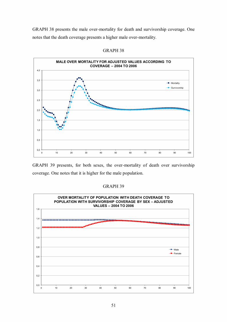
GRAPH 38 presents the male over-mortality for death and survivorship coverage. One

notes that the death coverage presents a higher male over-mortality.

GRAPH 38

0,0

0,5

1,0

1,5

2,0

2,5

3,0

3,5

4,0

0 10 20 30 40 50 60 70 80 90 100

MALE OVER MORTALITY FOR ADJUSTED VALUES ACCORDING TO COVERAGE – 2004 TO 2006

Mortality

Survivorship

GRAPH 39 presents, for both sexes, the over-mortality of death over survivorship

coverage. One notes that it is higher for the male population.

GRAPH 39

0,0

0,2

0,4

0,6

0,8

1,0

1,2

1,4

1,6

0 10 20 30 40 50 60 70 80 90 100

OVER MORTALITY OF POPULATION WITH DEATH COVERAGE TO POPULATION WITH SURVIVORSHIP COVERAGE BY SEX – ADJUSTED

VALUES – 2004 TO 2006

Male

Female

52

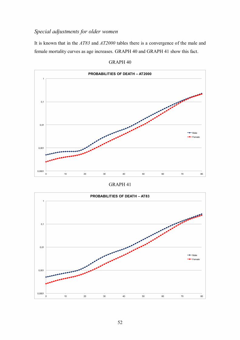
Special adjustments for older women It is known that in the AT83 and AT2000 tables there is a convergence of the male and

female mortality curves as age increases. GRAPH 40 and GRAPH 41 show this fact.

GRAPH 40

0,0001

0,001

0,01

0,1

1

0 10 20 30 40 50 60 70 80

PROBABILITIES OF DEATH – AT2000

Male

Female

GRAPH 41

0,0001

0,001

0,01

0,1

1

0 10 20 30 40 50 60 70 80

PROBABILITIES OF DEATH – AT83

Male

Female

53

Moreover, despite the fact that life expectancy at birth for women is higher than for

men, for older ages (90 and over), the mortality rates for both sexes tend to converge,

for most developed societies, for example France, Germany, United Kingdom, Russia,

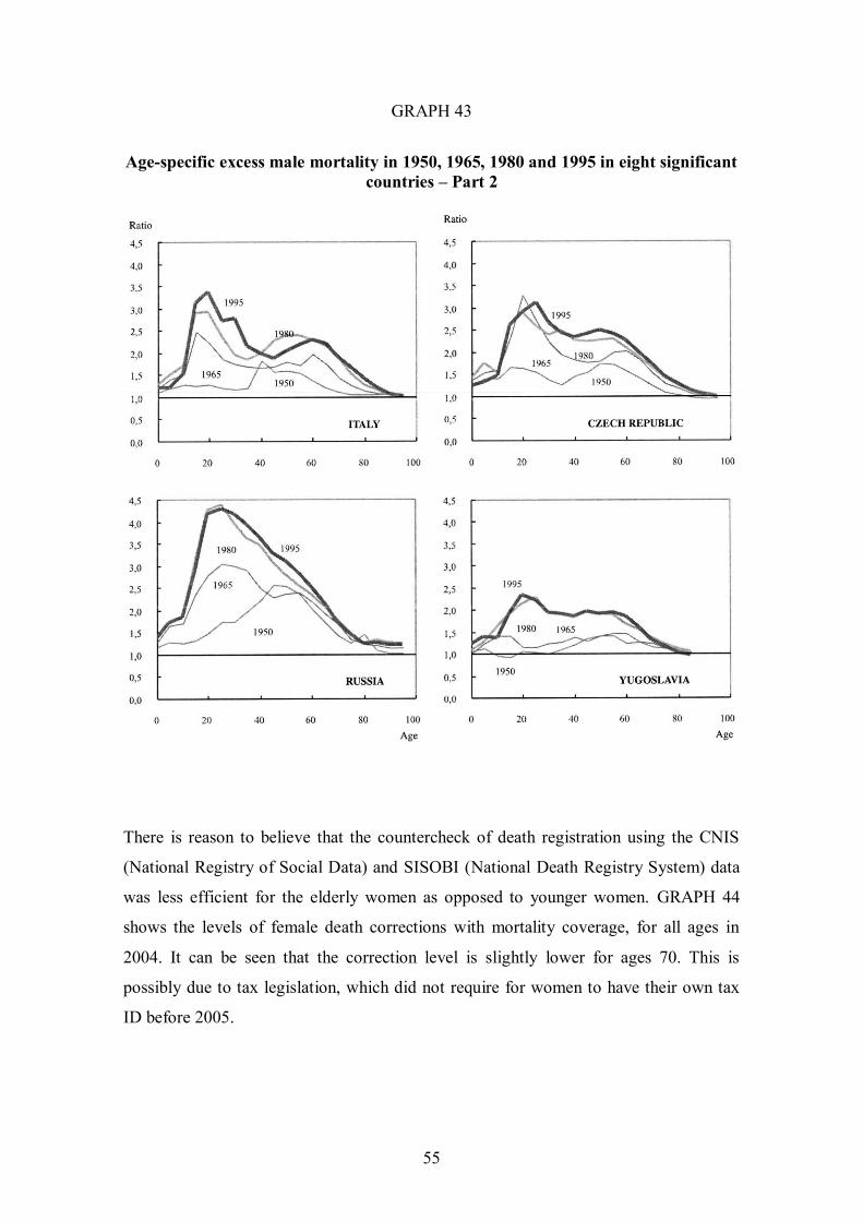
Czech Republic and Italy since 1950. As it occurs in the AT tables (see GRAPH 42 and

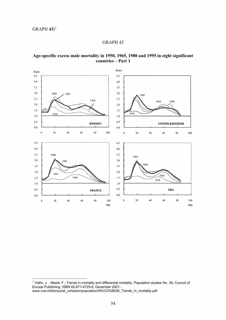
54

GRAPH 43)1

GRAPH 42

Age-specific excess male mortality in 1950, 1965, 1980 and 1995 in eight significant countries – Part 1

1 Vallin, J. , Meslé, F.; Trends in mortality and differential mortality, Population studies No. 36, Council of Europe Publishing, ISBN 92-871-4725-6, December 2001 - www.coe.int/t/e/social_cohesion/population/N%C2%B036_Trends_in_mortality.pdf

55

GRAPH 43

Age-specific excess male mortality in 1950, 1965, 1980 and 1995 in eight significant countries – Part 2

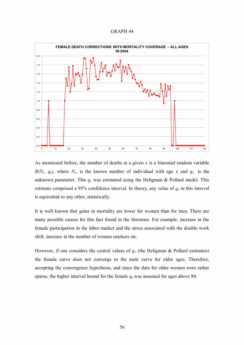
There is reason to believe that the countercheck of death registration using the CNIS

(National Registry of Social Data) and SISOBI (National Death Registry System) data

was less efficient for the elderly women as opposed to younger women. GRAPH 44

shows the levels of female death corrections with mortality coverage, for all ages in

2004. It can be seen that the correction level is slightly lower for ages 70. This is

possibly due to tax legislation, which did not require for women to have their own tax

ID before 2005.

56

GRAPH 44

0,0

0,2

0,4

0,6

0,8

1,0

1,2

1,4

1,6

1,8

2,0

0 10 20 30 40 50 60 70 80 90 100 110 120

FEMALE DEATH CORRECTIONS WITH MORTALITY COVERAGE – ALL AGES IN 2004

As mentioned before, the number of deaths at a given x is a binomial random variable

B(Nx, qx), where Nx, is the known number of individual with age x and qx is the

unknown parameter. This qx was estimated using the Heligman & Pollard model. This

estimate comprised a 95% confidence interval. In theory, any value of qx in this interval

is equivalent to any other, statistically.

It is well known that gains in mortality are lower for women than for men. There are

many possible causes for this fact found in the literature. For example, increase in the

female participation in the labor market and the stress associated with the double work

shift, increase in the number of women smokers etc.

However, if one considers the central values of qx (the Heligman & Pollard estimates)

the female curve does not converge to the male curve for older ages. Therefore,

accepting the convergence hypothesis, and since the data for older women were rather

sparse, the higher interval bound for the female qx was assumed for ages above 80.

57

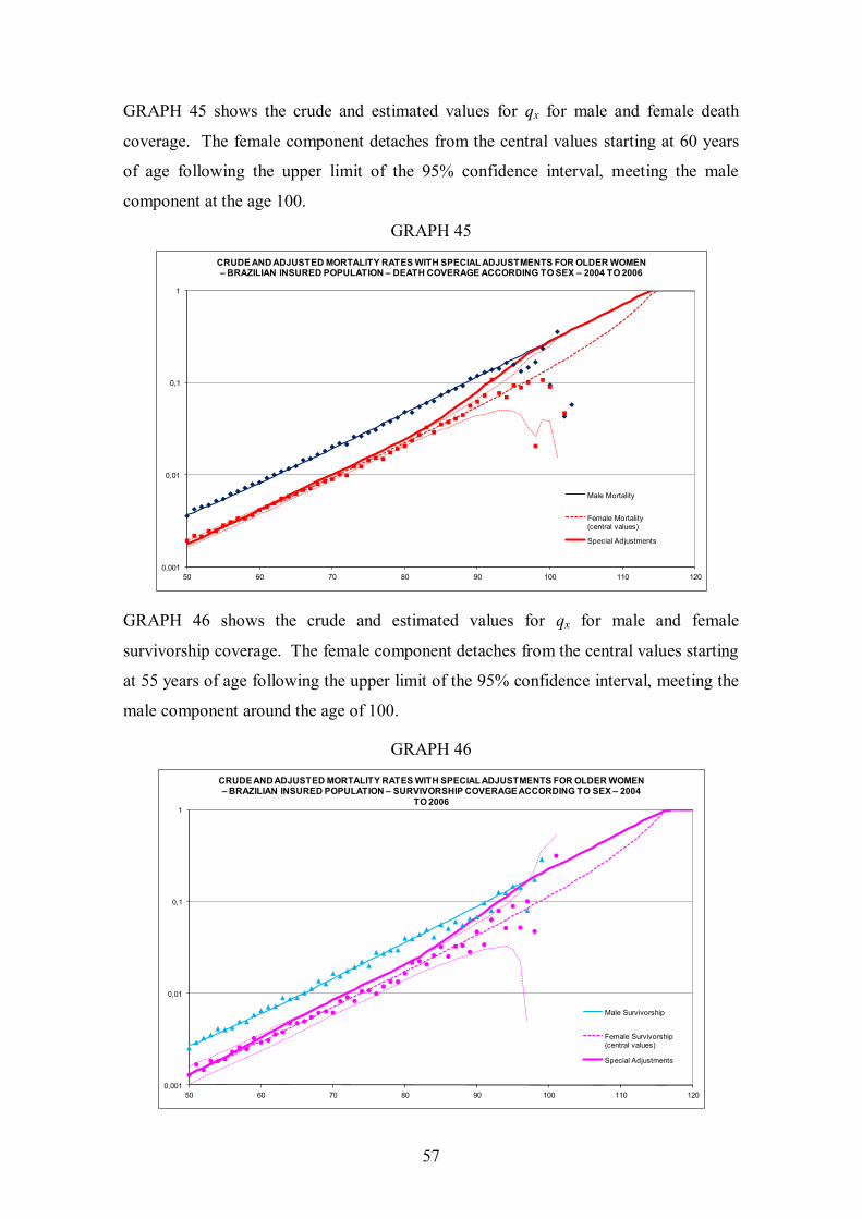
GRAPH 45 shows the crude and estimated values for qx for male and female death

coverage. The female component detaches from the central values starting at 60 years

of age following the upper limit of the 95% confidence interval, meeting the male

component at the age 100.

GRAPH 45

0,001

0,01

0,1

1

50 60 70 80 90 100 110 120

CRUDE AND ADJUSTED MORTALITY RATES WITH SPECIAL ADJUSTMENTS FOR OLDER WOMEN – BRAZILIAN INSURED POPULATION – DEATH COVERAGE ACCORDING TO SEX – 2004 TO 2006

Male Mortality

Female Mortality (central values)

Special Adjustments

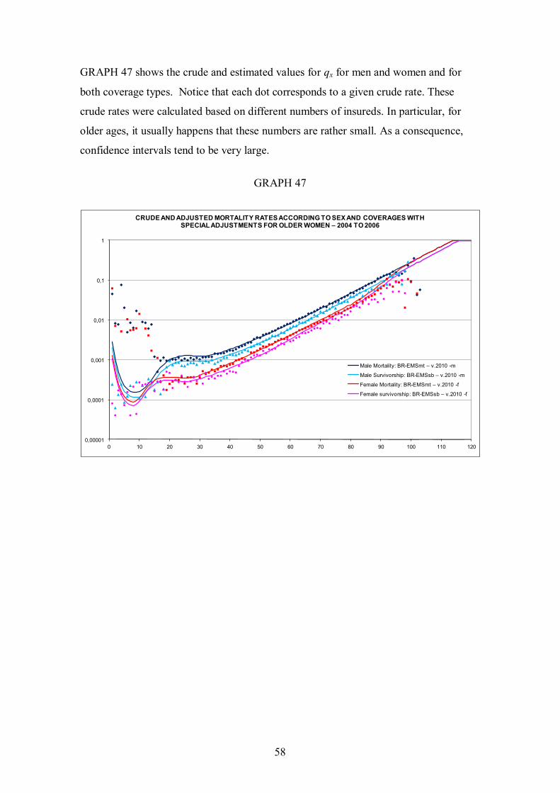
GRAPH 46 shows the crude and estimated values for qx for male and female

survivorship coverage. The female component detaches from the central values starting

at 55 years of age following the upper limit of the 95% confidence interval, meeting the

male component around the age of 100.

GRAPH 46

0,001

0,01

0,1

1

50 60 70 80 90 100 110 120

CRUDE AND ADJUSTED MORTALITY RATES WITH SPECIAL ADJUSTMENTS FOR OLDER WOMEN – BRAZILIAN INSURED POPULATION – SURVIVORSHIP COVERAGE ACCORDING TO SEX – 2004

TO 2006

Male Survivorship

Female Survivorship (central values)

Special Adjustments

58

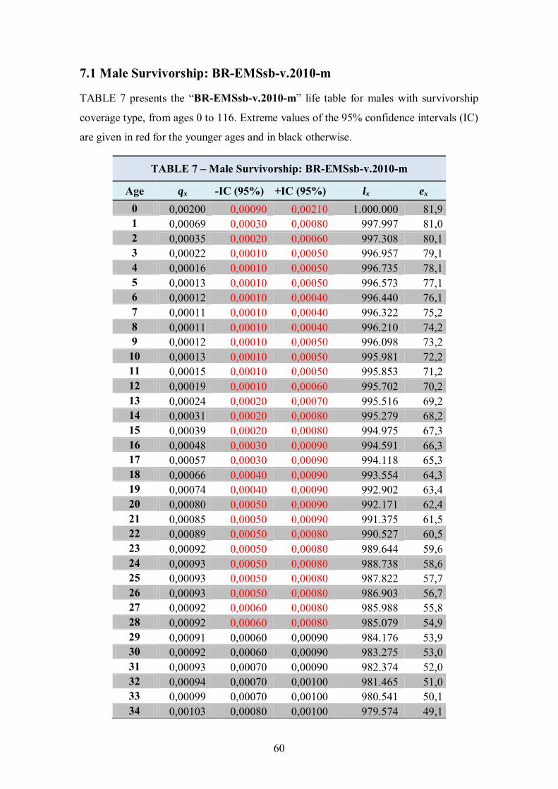
GRAPH 47 shows the crude and estimated values for qx for men and women and for

both coverage types. Notice that each dot corresponds to a given crude rate. These

crude rates were calculated based on different numbers of insureds. In particular, for

older ages, it usually happens that these numbers are rather small. As a consequence,

confidence intervals tend to be very large.

GRAPH 47

0,00001

0,0001

0,001

0,01

0,1

1

0 10 20 30 40 50 60 70 80 90 100 110 120

CRUDE AND ADJUSTED MORTALITY RATES ACCORDING TO SEX AND COVERAGES WITH SPECIAL ADJUSTMENTS FOR OLDER WOMEN – 2004 TO 2006

Male Mortality: BR-EMSmt – v.2010 -m

Male Survivorship: BR-EMSsb – v.2010 -m

Female Mortality: BR-EMSmt – v.2010 -f

Female survivorship: BR-EMSsb – v.2010 -f

59

CHAPTER 7 – BR-EMS TABLES

The adjusted tables, denominated “Experiência do Mercado Segurador Brasileiro –

BR-EMS”, presents variants classified according to coverage type and sex. The given

names of these variants follow the usual life table naming procedure, coverage type –

“sb” for survivorship and “mt” for mortality – and sex.

Although the life tables concern the death experience for the years 2004 to 2006,

centered in 2005, they were officially adopted, as standard tables, by SUSEP (Circular

SUPERINTENDÊNCIA DE SEGUROS PRIVADOS – SUSEP, nº 402, 18.03.2010 -

D.O.U.: 19.03.2010), and named the 2010 version of the BR-EMS.

Hence, we have the following variants of the BR-EMS.

BR-EMSsb-v.2010-m BR-EMSsb-v.2010-f

BR-EMSmt-v.2010-m BR-EMSmt-v.2010-f

Each variant comprises with the following parameters:

qx – probability (or rate) of death between ages x and x+1;

lx – number of living at age x;

ex – life expectancy at age x;

+IC (95%) – upper bound of 95% confidence interval and

-IC (95%) – lower bound of 95% confidence interval.

Confidence intervals were obtained using the normal approximation to the binomial

distribution. Hence negative values are not to be considered.

60

7.1 Male Survivorship: BR-EMSsb-v.2010-m

TABLE 7 presents the “BR-EMSsb-v.2010-m” life table for males with survivorship

coverage type, from ages 0 to 116. Extreme values of the 95% confidence intervals (IC)

are given in red for the younger ages and in black otherwise.

TABLE 7 – Male Survivorship: BR-EMSsb-v.2010-m

Age qx -IC (95%) +IC (95%) lx ex

0 0,00200 0,00090 0,00210 1.000.000 81,9 1 0,00069 0,00030 0,00080 997.997 81,0 2 0,00035 0,00020 0,00060 997.308 80,1 3 0,00022 0,00010 0,00050 996.957 79,1 4 0,00016 0,00010 0,00050 996.735 78,1 5 0,00013 0,00010 0,00050 996.573 77,1 6 0,00012 0,00010 0,00040 996.440 76,1 7 0,00011 0,00010 0,00040 996.322 75,2 8 0,00011 0,00010 0,00040 996.210 74,2 9 0,00012 0,00010 0,00050 996.098 73,2

10 0,00013 0,00010 0,00050 995.981 72,2 11 0,00015 0,00010 0,00050 995.853 71,2 12 0,00019 0,00010 0,00060 995.702 70,2 13 0,00024 0,00020 0,00070 995.516 69,2 14 0,00031 0,00020 0,00080 995.279 68,2 15 0,00039 0,00020 0,00080 994.975 67,3 16 0,00048 0,00030 0,00090 994.591 66,3 17 0,00057 0,00030 0,00090 994.118 65,3 18 0,00066 0,00040 0,00090 993.554 64,3 19 0,00074 0,00040 0,00090 992.902 63,4 20 0,00080 0,00050 0,00090 992.171 62,4 21 0,00085 0,00050 0,00090 991.375 61,5 22 0,00089 0,00050 0,00080 990.527 60,5 23 0,00092 0,00050 0,00080 989.644 59,6 24 0,00093 0,00050 0,00080 988.738 58,6 25 0,00093 0,00050 0,00080 987.822 57,7 26 0,00093 0,00050 0,00080 986.903 56,7 27 0,00092 0,00060 0,00080 985.988 55,8 28 0,00092 0,00060 0,00080 985.079 54,9 29 0,00091 0,00060 0,00090 984.176 53,9 30 0,00092 0,00060 0,00090 983.275 53,0 31 0,00093 0,00070 0,00090 982.374 52,0 32 0,00094 0,00070 0,00100 981.465 51,0 33 0,00099 0,00070 0,00100 980.541 50,1 34 0,00103 0,00080 0,00100 979.574 49,1

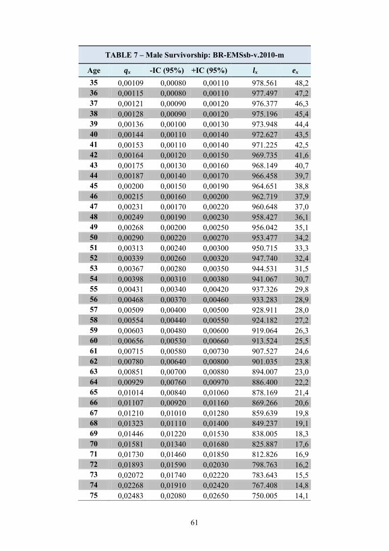
61

TABLE 7 – Male Survivorship: BR-EMSsb-v.2010-m

Age qx -IC (95%) +IC (95%) lx ex

35 0,00109 0,00080 0,00110 978.561 48,2 36 0,00115 0,00080 0,00110 977.497 47,2 37 0,00121 0,00090 0,00120 976.377 46,3 38 0,00128 0,00090 0,00120 975.196 45,4 39 0,00136 0,00100 0,00130 973.948 44,4 40 0,00144 0,00110 0,00140 972.627 43,5 41 0,00153 0,00110 0,00140 971.225 42,5 42 0,00164 0,00120 0,00150 969.735 41,6 43 0,00175 0,00130 0,00160 968.149 40,7 44 0,00187 0,00140 0,00170 966.458 39,7 45 0,00200 0,00150 0,00190 964.651 38,8 46 0,00215 0,00160 0,00200 962.719 37,9 47 0,00231 0,00170 0,00220 960.648 37,0 48 0,00249 0,00190 0,00230 958.427 36,1 49 0,00268 0,00200 0,00250 956.042 35,1 50 0,00290 0,00220 0,00270 953.477 34,2 51 0,00313 0,00240 0,00300 950.715 33,3 52 0,00339 0,00260 0,00320 947.740 32,4 53 0,00367 0,00280 0,00350 944.531 31,5 54 0,00398 0,00310 0,00380 941.067 30,7 55 0,00431 0,00340 0,00420 937.326 29,8 56 0,00468 0,00370 0,00460 933.283 28,9 57 0,00509 0,00400 0,00500 928.911 28,0 58 0,00554 0,00440 0,00550 924.182 27,2 59 0,00603 0,00480 0,00600 919.064 26,3 60 0,00656 0,00530 0,00660 913.524 25,5 61 0,00715 0,00580 0,00730 907.527 24,6 62 0,00780 0,00640 0,00800 901.035 23,8 63 0,00851 0,00700 0,00880 894.007 23,0 64 0,00929 0,00760 0,00970 886.400 22,2 65 0,01014 0,00840 0,01060 878.169 21,4 66 0,01107 0,00920 0,01160 869.266 20,6 67 0,01210 0,01010 0,01280 859.639 19,8 68 0,01323 0,01110 0,01400 849.237 19,1 69 0,01446 0,01220 0,01530 838.005 18,3 70 0,01581 0,01340 0,01680 825.887 17,6 71 0,01730 0,01460 0,01850 812.826 16,9 72 0,01893 0,01590 0,02030 798.763 16,2 73 0,02072 0,01740 0,02220 783.643 15,5 74 0,02268 0,01910 0,02420 767.408 14,8 75 0,02483 0,02080 0,02650 750.005 14,1

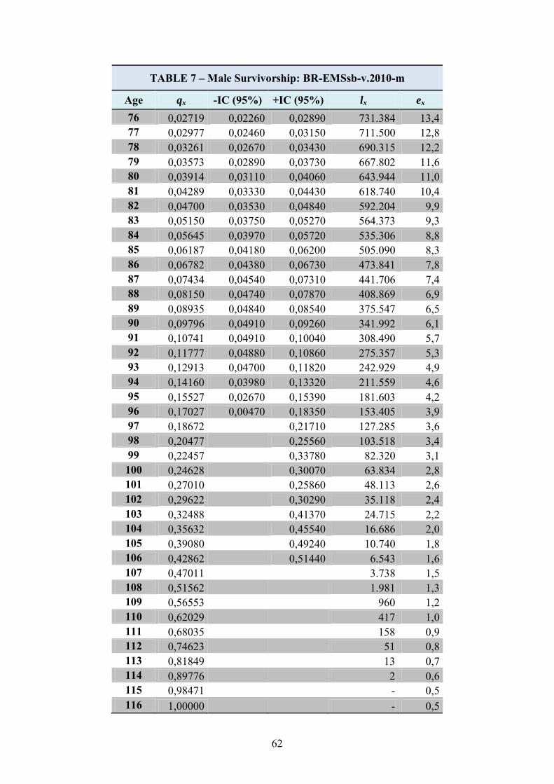
62

TABLE 7 – Male Survivorship: BR-EMSsb-v.2010-m

Age qx -IC (95%) +IC (95%) lx ex

76 0,02719 0,02260 0,02890 731.384 13,4 77 0,02977 0,02460 0,03150 711.500 12,8 78 0,03261 0,02670 0,03430 690.315 12,2 79 0,03573 0,02890 0,03730 667.802 11,6 80 0,03914 0,03110 0,04060 643.944 11,0 81 0,04289 0,03330 0,04430 618.740 10,4 82 0,04700 0,03530 0,04840 592.204 9,9 83 0,05150 0,03750 0,05270 564.373 9,3 84 0,05645 0,03970 0,05720 535.306 8,8 85 0,06187 0,04180 0,06200 505.090 8,3 86 0,06782 0,04380 0,06730 473.841 7,8 87 0,07434 0,04540 0,07310 441.706 7,4 88 0,08150 0,04740 0,07870 408.869 6,9 89 0,08935 0,04840 0,08540 375.547 6,5 90 0,09796 0,04910 0,09260 341.992 6,1 91 0,10741 0,04910 0,10040 308.490 5,7 92 0,11777 0,04880 0,10860 275.357 5,3 93 0,12913 0,04700 0,11820 242.929 4,9 94 0,14160 0,03980 0,13320 211.559 4,6 95 0,15527 0,02670 0,15390 181.603 4,2 96 0,17027 0,00470 0,18350 153.405 3,9 97 0,18672

0,21710 127.285 3,6

98 0,20477

0,25560 103.518 3,4 99 0,22457

0,33780 82.320 3,1

100 0,24628

0,30070 63.834 2,8 101 0,27010

0,25860 48.113 2,6

102 0,29622

0,30290 35.118 2,4 103 0,32488

0,41370 24.715 2,2

104 0,35632

0,45540 16.686 2,0 105 0,39080

0,49240 10.740 1,8

106 0,42862

0,51440 6.543 1,6 107 0,47011

3.738 1,5

108 0,51562

1.981 1,3 109 0,56553

960 1,2

110 0,62029

417 1,0 111 0,68035

158 0,9

112 0,74623

51 0,8 113 0,81849

13 0,7

114 0,89776

2 0,6 115 0,98471

- 0,5

116 1,00000

- 0,5

63

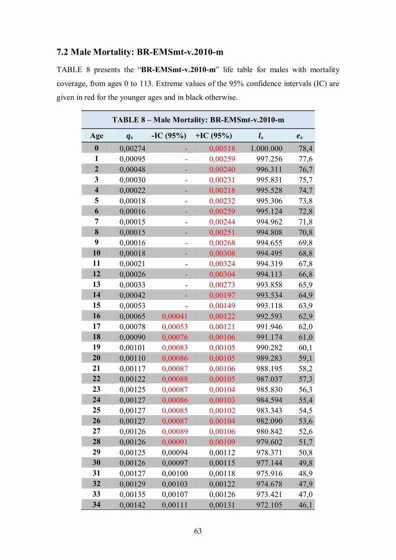
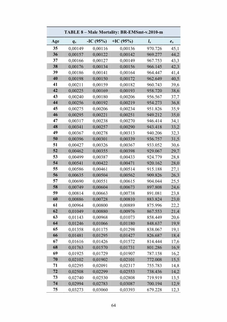
7.2 Male Mortality: BR-EMSmt-v.2010-m

TABLE 8 presents the “BR-EMSmt-v.2010-m” life table for males with mortality

coverage, from ages 0 to 113. Extreme values of the 95% confidence intervals (IC) are

given in red for the younger ages and in black otherwise.

TABLE 8 – Male Mortality: BR-EMSmt-v.2010-m

Age qx -IC (95%) +IC (95%) lx ex

0 0,00274 - 0,00518 1.000.000 78,4 1 0,00095 - 0,00259 997.256 77,6 2 0,00048 - 0,00240 996.311 76,7 3 0,00030 - 0,00231 995.831 75,7 4 0,00022 - 0,00218 995.528 74,7 5 0,00018 - 0,00232 995.306 73,8 6 0,00016 - 0,00259 995.124 72,8 7 0,00015 - 0,00244 994.962 71,8 8 0,00015 - 0,00251 994.808 70,8 9 0,00016 - 0,00268 994.655 69,8

10 0,00018 - 0,00308 994.495 68,8 11 0,00021 - 0,00324 994.319 67,8 12 0,00026 - 0,00304 994.113 66,8 13 0,00033 - 0,00273 993.858 65,9 14 0,00042 - 0,00197 993.534 64,9 15 0,00053 - 0,00149 993.118 63,9 16 0,00065 0,00041 0,00122 992.593 62,9 17 0,00078 0,00053 0,00121 991.946 62,0 18 0,00090 0,00076 0,00106 991.174 61,0 19 0,00101 0,00083 0,00105 990.282 60,1 20 0,00110 0,00086 0,00105 989.283 59,1 21 0,00117 0,00087 0,00106 988.195 58,2 22 0,00122 0,00088 0,00105 987.037 57,3 23 0,00125 0,00087 0,00104 985.830 56,3 24 0,00127 0,00086 0,00103 984.594 55,4 25 0,00127 0,00085 0,00102 983.343 54,5 26 0,00127 0,00087 0,00104 982.090 53,6 27 0,00126 0,00089 0,00106 980.842 52,6 28 0,00126 0,00091 0,00109 979.602 51,7 29 0,00125 0,00094 0,00112 978.371 50,8 30 0,00126 0,00097 0,00115 977.144 49,8 31 0,00127 0,00100 0,00118 975.916 48,9 32 0,00129 0,00103 0,00122 974.678 47,9 33 0,00135 0,00107 0,00126 973.421 47,0 34 0,00142 0,00111 0,00131 972.105 46,1

64

TABLE 8 – Male Mortality: BR-EMSmt-v.2010-m

Age qx -IC (95%) +IC (95%) lx ex

35 0,00149 0,00116 0,00136 970.726 45,1 36 0,00157 0,00122 0,00142 969.277 44,2 37 0,00166 0,00127 0,00149 967.753 43,3 38 0,00176 0,00134 0,00156 966.145 42,3 39 0,00186 0,00141 0,00164 964.447 41,4 40 0,00198 0,00150 0,00172 962.649 40,5 41 0,00211 0,00159 0,00182 960.743 39,6 42 0,00225 0,00169 0,00193 958.720 38,6 43 0,00240 0,00180 0,00206 956.567 37,7 44 0,00256 0,00192 0,00219 954.273 36,8 45 0,00275 0,00206 0,00234 951.826 35,9 46 0,00295 0,00221 0,00251 949.212 35,0 47 0,00317 0,00238 0,00270 946.414 34,1 48 0,00341 0,00257 0,00290 943.418 33,2 49 0,00367 0,00278 0,00313 940.206 32,3 50 0,00396 0,00301 0,00339 936.757 31,5 51 0,00427 0,00326 0,00367 933.052 30,6 52 0,00462 0,00355 0,00398 929.067 29,7 53 0,00499 0,00387 0,00433 924.779 28,8 54 0,00541 0,00422 0,00471 920.162 28,0 55 0,00586 0,00461 0,00514 915.188 27,1 56 0,00635 0,00504 0,00562 909.826 26,3 57 0,00690 0,00551 0,00615 904.044 25,5 58 0,00749 0,00604 0,00673 897.808 24,6 59 0,00814 0,00663 0,00738 891.081 23,8 60 0,00886 0,00728 0,00810 883.824 23,0 61 0,00964 0,00800 0,00889 875.996 22,2 62 0,01049 0,00880 0,00976 867.553 21,4 63 0,01143 0,00968 0,01073 858.449 20,6 64 0,01246 0,01066 0,01180 848.637 19,9 65 0,01358 0,01175 0,01298 838.067 19,1 66 0,01481 0,01295 0,01427 826.687 18,4 67 0,01616 0,01426 0,01572 814.444 17,6 68 0,01763 0,01570 0,01731 801.286 16,9 69 0,01925 0,01729 0,01907 787.158 16,2 70 0,02102 0,01902 0,02101 772.008 15,5 71 0,02295 0,02091 0,02317 755.783 14,8 72 0,02508 0,02299 0,02553 738.436 14,2 73 0,02740 0,02530 0,02808 719.919 13,5 74 0,02994 0,02783 0,03087 700.194 12,9 75 0,03273 0,03060 0,03393 679.228 12,3

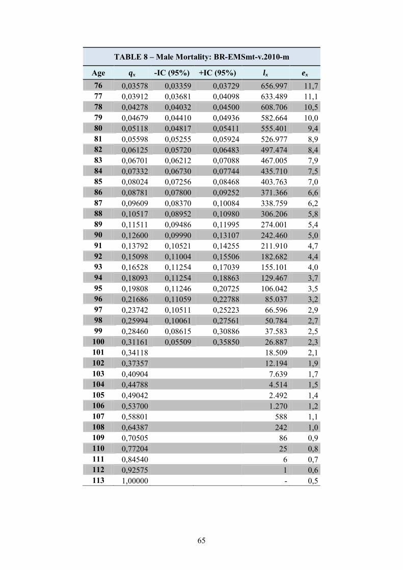
65

TABLE 8 – Male Mortality: BR-EMSmt-v.2010-m

Age qx -IC (95%) +IC (95%) lx ex

76 0,03578 0,03359 0,03729 656.997 11,7 77 0,03912 0,03681 0,04098 633.489 11,1 78 0,04278 0,04032 0,04500 608.706 10,5 79 0,04679 0,04410 0,04936 582.664 10,0 80 0,05118 0,04817 0,05411 555.401 9,4 81 0,05598 0,05255 0,05924 526.977 8,9 82 0,06125 0,05720 0,06483 497.474 8,4 83 0,06701 0,06212 0,07088 467.005 7,9 84 0,07332 0,06730 0,07744 435.710 7,5 85 0,08024 0,07256 0,08468 403.763 7,0 86 0,08781 0,07800 0,09252 371.366 6,6 87 0,09609 0,08370 0,10084 338.759 6,2 88 0,10517 0,08952 0,10980 306.206 5,8 89 0,11511 0,09486 0,11995 274.001 5,4 90 0,12600 0,09990 0,13107 242.460 5,0 91 0,13792 0,10521 0,14255 211.910 4,7 92 0,15098 0,11004 0,15506 182.682 4,4 93 0,16528 0,11254 0,17039 155.101 4,0 94 0,18093 0,11254 0,18863 129.467 3,7 95 0,19808 0,11246 0,20725 106.042 3,5 96 0,21686 0,11059 0,22788 85.037 3,2 97 0,23742 0,10511 0,25223 66.596 2,9 98 0,25994 0,10061 0,27561 50.784 2,7 99 0,28460 0,08615 0,30886 37.583 2,5 100 0,31161 0,05509 0,35850 26.887 2,3 101 0,34118

18.509 2,1

102 0,37357

12.194 1,9 103 0,40904

7.639 1,7

104 0,44788

4.514 1,5 105 0,49042

2.492 1,4

106 0,53700

1.270 1,2 107 0,58801

588 1,1

108 0,64387

242 1,0 109 0,70505

86 0,9

110 0,77204

25 0,8 111 0,84540

6 0,7

112 0,92575

1 0,6 113 1,00000

- 0,5

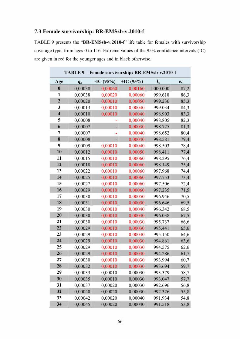
66

7.3 Female survivorship: BR-EMSsb-v.2010-f

TABLE 9 presents the “BR-EMSsb-v.2010-f” life table for females with survivorship

coverage type, from ages 0 to 116. Extreme values of the 95% confidence intervals (IC)

are given in red for the younger ages and in black otherwise.

TABLE 9 – Female survivorship: BR-EMSsb-v.2010-f

Age qx -IC (95%) +IC (95%) lx ex

0 0,00038 0,00060 0,00160 1.000.000 87,2 1 0,00038 0,00020 0,00060 999.618 86,3 2 0,00020 0,00010 0,00050 999.236 85,3 3 0,00013 0,00010 0,00040 999.034 84,3 4 0,00010 0,00010 0,00040 998.903 83,3 5 0,00008 - 0,00040 998.805 82,3 6 0,00007 - 0,00030 998.725 81,3 7 0,00007 - 0,00040 998.652 80,4 8 0,00008 - 0,00040 998.581 79,4 9 0,00009 0,00010 0,00040 998.503 78,4 10 0,00012 0,00010 0,00050 998.411 77,4 11 0,00015 0,00010 0,00060 998.295 76,4 12 0,00018 0,00010 0,00060 998.149 75,4 13 0,00022 0,00010 0,00060 997.968 74,4 14 0,00025 0,00010 0,00060 997.753 73,4 15 0,00027 0,00010 0,00060 997.506 72,4 16 0,00029 0,00010 0,00060 997.235 71,5 17 0,00030 0,00010 0,00050 996.946 70,5 18 0,00031 0,00010 0,00050 996.646 69,5 19 0,00030 0,00010 0,00040 996.342 68,5 20 0,00030 0,00010 0,00040 996.038 67,5 21 0,00030 0,00010 0,00030 995.737 66,6 22 0,00029 0,00010 0,00030 995.441 65,6 23 0,00029 0,00010 0,00030 995.150 64,6 24 0,00029 0,00010 0,00030 994.861 63,6 25 0,00029 0,00010 0,00030 994.575 62,6 26 0,00029 0,00010 0,00030 994.286 61,7 27 0,00030 0,00010 0,00030 993.994 60,7 28 0,00032 0,00010 0,00030 993.694 59,7 29 0,00033 0,00010 0,00030 993.379 58,7 30 0,00035 0,00010 0,00030 993.047 57,7 31 0,00037 0,00020 0,00030 992.696 56,8 32 0,00040 0,00020 0,00030 992.326 55,8 33 0,00042 0,00020 0,00040 991.934 54,8 34 0,00045 0,00020 0,00040 991.518 53,8

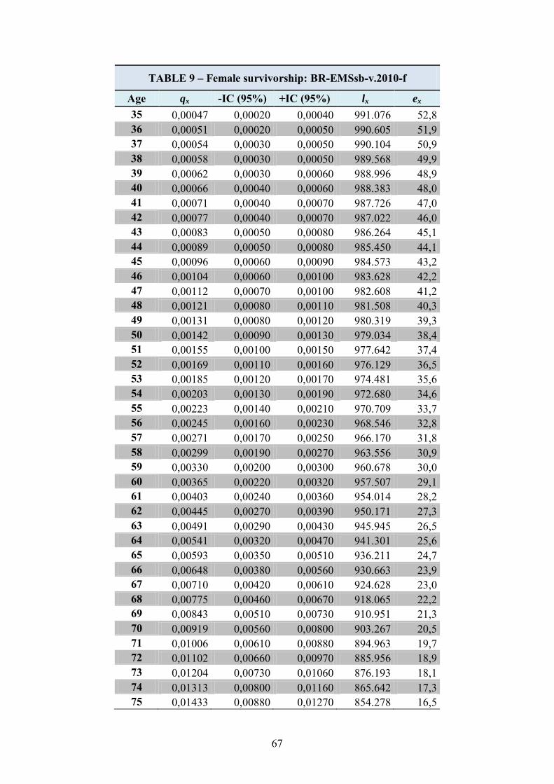
67

TABLE 9 – Female survivorship: BR-EMSsb-v.2010-f

Age qx -IC (95%) +IC (95%) lx ex

35 0,00047 0,00020 0,00040 991.076 52,8 36 0,00051 0,00020 0,00050 990.605 51,9 37 0,00054 0,00030 0,00050 990.104 50,9 38 0,00058 0,00030 0,00050 989.568 49,9 39 0,00062 0,00030 0,00060 988.996 48,9 40 0,00066 0,00040 0,00060 988.383 48,0 41 0,00071 0,00040 0,00070 987.726 47,0 42 0,00077 0,00040 0,00070 987.022 46,0 43 0,00083 0,00050 0,00080 986.264 45,1 44 0,00089 0,00050 0,00080 985.450 44,1 45 0,00096 0,00060 0,00090 984.573 43,2 46 0,00104 0,00060 0,00100 983.628 42,2 47 0,00112 0,00070 0,00100 982.608 41,2 48 0,00121 0,00080 0,00110 981.508 40,3 49 0,00131 0,00080 0,00120 980.319 39,3 50 0,00142 0,00090 0,00130 979.034 38,4 51 0,00155 0,00100 0,00150 977.642 37,4 52 0,00169 0,00110 0,00160 976.129 36,5 53 0,00185 0,00120 0,00170 974.481 35,6 54 0,00203 0,00130 0,00190 972.680 34,6 55 0,00223 0,00140 0,00210 970.709 33,7 56 0,00245 0,00160 0,00230 968.546 32,8 57 0,00271 0,00170 0,00250 966.170 31,8 58 0,00299 0,00190 0,00270 963.556 30,9 59 0,00330 0,00200 0,00300 960.678 30,0 60 0,00365 0,00220 0,00320 957.507 29,1 61 0,00403 0,00240 0,00360 954.014 28,2 62 0,00445 0,00270 0,00390 950.171 27,3 63 0,00491 0,00290 0,00430 945.945 26,5 64 0,00541 0,00320 0,00470 941.301 25,6 65 0,00593 0,00350 0,00510 936.211 24,7 66 0,00648 0,00380 0,00560 930.663 23,9 67 0,00710 0,00420 0,00610 924.628 23,0 68 0,00775 0,00460 0,00670 918.065 22,2 69 0,00843 0,00510 0,00730 910.951 21,3 70 0,00919 0,00560 0,00800 903.267 20,5 71 0,01006 0,00610 0,00880 894.963 19,7 72 0,01102 0,00660 0,00970 885.956 18,9 73 0,01204 0,00730 0,01060 876.193 18,1 74 0,01313 0,00800 0,01160 865.642 17,3 75 0,01433 0,00880 0,01270 854.278 16,5

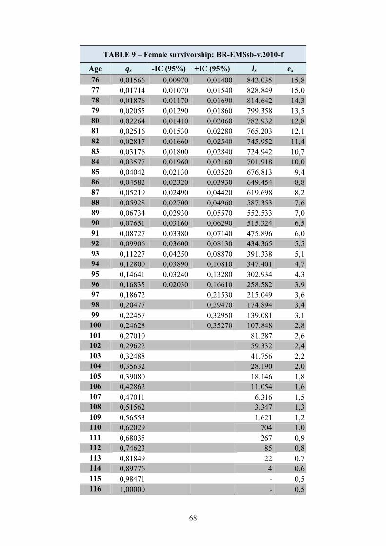
68

TABLE 9 – Female survivorship: BR-EMSsb-v.2010-f

Age qx -IC (95%) +IC (95%) lx ex

76 0,01566 0,00970 0,01400 842.035 15,8 77 0,01714 0,01070 0,01540 828.849 15,0 78 0,01876 0,01170 0,01690 814.642 14,3 79 0,02055 0,01290 0,01860 799.358 13,5 80 0,02264 0,01410 0,02060 782.932 12,8 81 0,02516 0,01530 0,02280 765.203 12,1 82 0,02817 0,01660 0,02540 745.952 11,4 83 0,03176 0,01800 0,02840 724.942 10,7 84 0,03577 0,01960 0,03160 701.918 10,0 85 0,04042 0,02130 0,03520 676.813 9,4 86 0,04582 0,02320 0,03930 649.454 8,8 87 0,05219 0,02490 0,04420 619.698 8,2 88 0,05928 0,02700 0,04960 587.353 7,6 89 0,06734 0,02930 0,05570 552.533 7,0 90 0,07651 0,03160 0,06290 515.324 6,5 91 0,08727 0,03380 0,07140 475.896 6,0 92 0,09906 0,03600 0,08130 434.365 5,5 93 0,11227 0,04250 0,08870 391.338 5,1 94 0,12800 0,03890 0,10810 347.401 4,7 95 0,14641 0,03240 0,13280 302.934 4,3 96 0,16835 0,02030 0,16610 258.582 3,9 97 0,18672

0,21530 215.049 3,6

98 0,20477

0,29470 174.894 3,4 99 0,22457

0,32950 139.081 3,1

100 0,24628

0,35270 107.848 2,8 101 0,27010

81.287 2,6

102 0,29622

59.332 2,4 103 0,32488

41.756 2,2

104 0,35632

28.190 2,0 105 0,39080

18.146 1,8

106 0,42862

11.054 1,6 107 0,47011

6.316 1,5

108 0,51562

3.347 1,3 109 0,56553

1.621 1,2

110 0,62029

704 1,0 111 0,68035

267 0,9

112 0,74623

85 0,8 113 0,81849

22 0,7

114 0,89776

4 0,6 115 0,98471

- 0,5

116 1,00000

- 0,5

69

7.4 Female Mortality: BR-EMSmt-v.2010-f

TABLE 10 presents the “BR-EMSmt-v.2010-f” life table for females with mortality

coverage, from ages 0 to 113. Extreme values of the 95% confidence intervals (IC) are

given in red for the younger ages and in black otherwise.

TABLE 10 – Female Mortality: BR-EMSmt-v.2010-f

Age qx -IC (95%) +IC (95%) lx ex

0 0,00128

0,00850 1.000.000 85,2 1 0,00046

0,00430 998.716 84,3

2 0,00025

0,00370 998.252 83,4 3 0,00016

0,00390 998.007 82,4

4 0,00012

0,00360 997.847 81,4 5 0,00010

0,00360 997.728 80,4

6 0,00009

0,00360 997.630 79,4 7 0,00009

0,00370 997.542 78,4

8 0,00009

0,00420 997.455 77,4 9 0,00011

0,00470 997.361 76,4

10 0,00014

0,00490 997.249 75,4 11 0,00018

0,00490 997.108 74,4

12 0,00022

0,00410 996.930 73,5 13 0,00026

0,00300 996.711 72,5

14 0,00030

0,00250 996.449 71,5 15 0,00033

0,00170 996.150 70,5

16 0,00035 0,00020 0,00120 995.820 69,5 17 0,00037 0,00030 0,00100 995.469 68,6 18 0,00037 0,00050 0,00070 995.105 67,6 19 0,00037 0,00050 0,00060 994.735 66,6 20 0,00037 0,00040 0,00060 994.366 65,6 21 0,00036 0,00040 0,00050 994.001 64,7 22 0,00036 0,00040 0,00050 993.642 63,7 23 0,00035 0,00040 0,00050 993.288 62,7 24 0,00035 0,00040 0,00050 992.938 61,7 25 0,00035 0,00040 0,00050 992.589 60,7 26 0,00036 0,00040 0,00050 992.239 59,8 27 0,00037 0,00040 0,00050 991.884 58,8 28 0,00039 0,00040 0,00050 991.520 57,8 29 0,00041 0,00040 0,00050 991.134 56,8 30 0,00044 0,00040 0,00060 990.723 55,9 31 0,00047 0,00040 0,00060 990.286 54,9 32 0,00050 0,00050 0,00060 989.820 53,9 33 0,00054 0,00050 0,00060 989.323 52,9

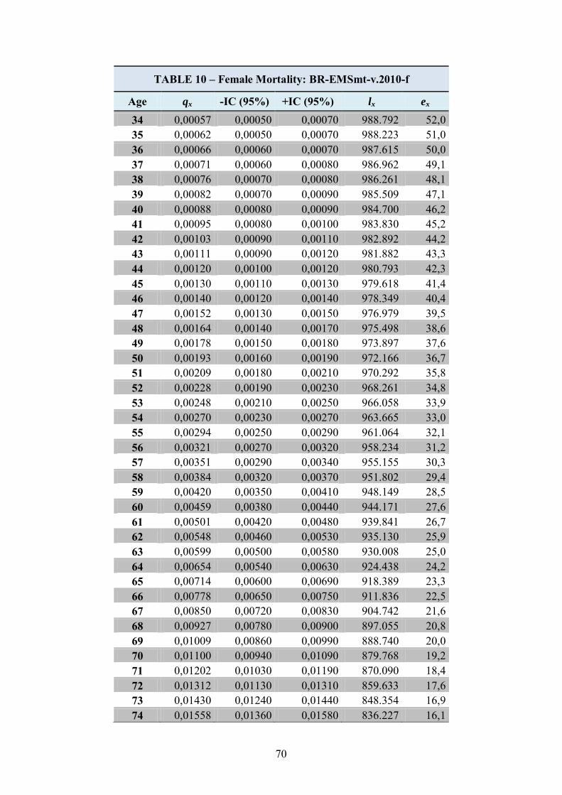
70

TABLE 10 – Female Mortality: BR-EMSmt-v.2010-f

Age qx -IC (95%) +IC (95%) lx ex

34 0,00057 0,00050 0,00070 988.792 52,0 35 0,00062 0,00050 0,00070 988.223 51,0 36 0,00066 0,00060 0,00070 987.615 50,0 37 0,00071 0,00060 0,00080 986.962 49,1 38 0,00076 0,00070 0,00080 986.261 48,1 39 0,00082 0,00070 0,00090 985.509 47,1 40 0,00088 0,00080 0,00090 984.700 46,2 41 0,00095 0,00080 0,00100 983.830 45,2 42 0,00103 0,00090 0,00110 982.892 44,2 43 0,00111 0,00090 0,00120 981.882 43,3 44 0,00120 0,00100 0,00120 980.793 42,3 45 0,00130 0,00110 0,00130 979.618 41,4 46 0,00140 0,00120 0,00140 978.349 40,4 47 0,00152 0,00130 0,00150 976.979 39,5 48 0,00164 0,00140 0,00170 975.498 38,6 49 0,00178 0,00150 0,00180 973.897 37,6 50 0,00193 0,00160 0,00190 972.166 36,7 51 0,00209 0,00180 0,00210 970.292 35,8 52 0,00228 0,00190 0,00230 968.261 34,8 53 0,00248 0,00210 0,00250 966.058 33,9 54 0,00270 0,00230 0,00270 963.665 33,0 55 0,00294 0,00250 0,00290 961.064 32,1 56 0,00321 0,00270 0,00320 958.234 31,2 57 0,00351 0,00290 0,00340 955.155 30,3 58 0,00384 0,00320 0,00370 951.802 29,4 59 0,00420 0,00350 0,00410 948.149 28,5 60 0,00459 0,00380 0,00440 944.171 27,6 61 0,00501 0,00420 0,00480 939.841 26,7 62 0,00548 0,00460 0,00530 935.130 25,9 63 0,00599 0,00500 0,00580 930.008 25,0 64 0,00654 0,00540 0,00630 924.438 24,2 65 0,00714 0,00600 0,00690 918.389 23,3 66 0,00778 0,00650 0,00750 911.836 22,5 67 0,00850 0,00720 0,00830 904.742 21,6 68 0,00927 0,00780 0,00900 897.055 20,8 69 0,01009 0,00860 0,00990 888.740 20,0 70 0,01100 0,00940 0,01090 879.768 19,2 71 0,01202 0,01030 0,01190 870.090 18,4 72 0,01312 0,01130 0,01310 859.633 17,6 73 0,01430 0,01240 0,01440 848.354 16,9 74 0,01558 0,01360 0,01580 836.227 16,1

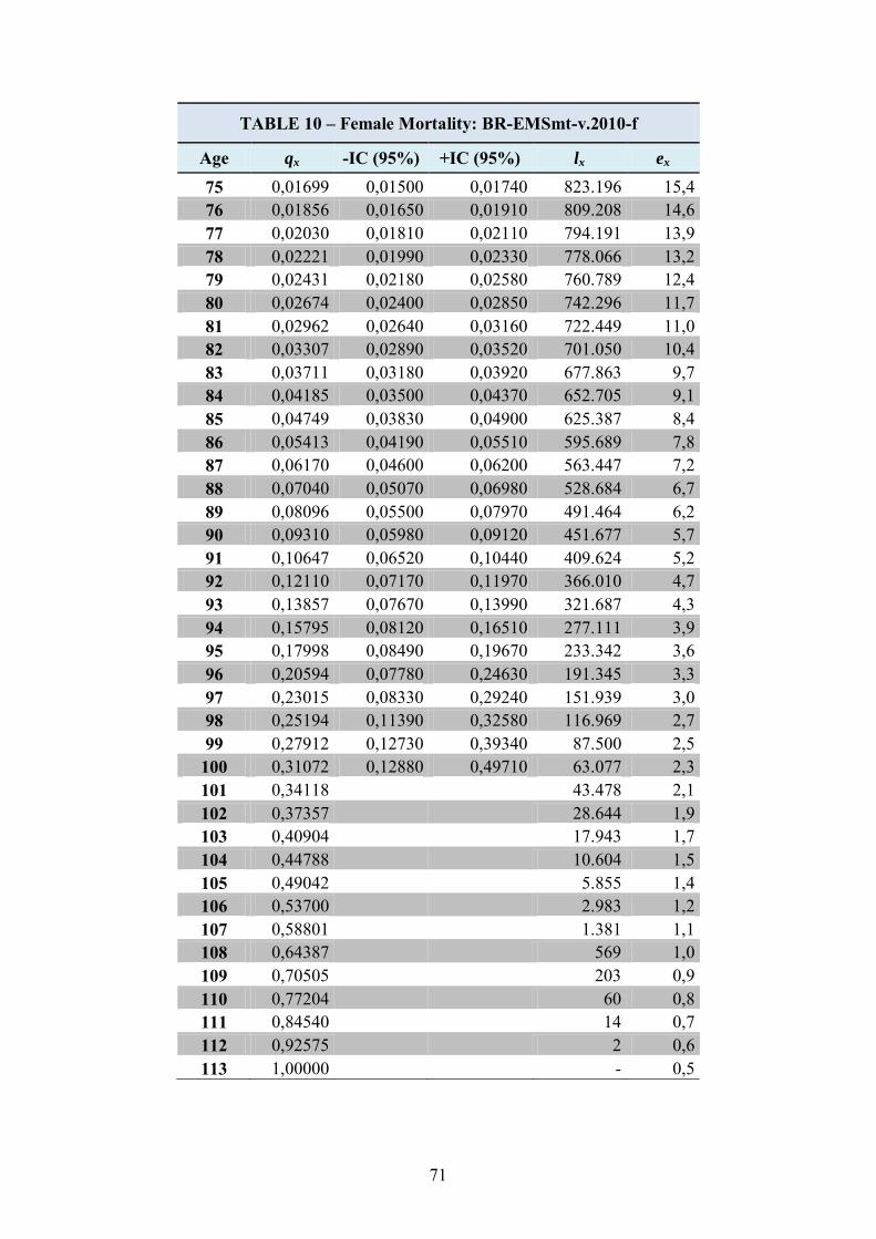
71

TABLE 10 – Female Mortality: BR-EMSmt-v.2010-f

Age qx -IC (95%) +IC (95%) lx ex

75 0,01699 0,01500 0,01740 823.196 15,4 76 0,01856 0,01650 0,01910 809.208 14,6 77 0,02030 0,01810 0,02110 794.191 13,9 78 0,02221 0,01990 0,02330 778.066 13,2 79 0,02431 0,02180 0,02580 760.789 12,4 80 0,02674 0,02400 0,02850 742.296 11,7 81 0,02962 0,02640 0,03160 722.449 11,0 82 0,03307 0,02890 0,03520 701.050 10,4 83 0,03711 0,03180 0,03920 677.863 9,7 84 0,04185 0,03500 0,04370 652.705 9,1 85 0,04749 0,03830 0,04900 625.387 8,4 86 0,05413 0,04190 0,05510 595.689 7,8 87 0,06170 0,04600 0,06200 563.447 7,2 88 0,07040 0,05070 0,06980 528.684 6,7 89 0,08096 0,05500 0,07970 491.464 6,2 90 0,09310 0,05980 0,09120 451.677 5,7 91 0,10647 0,06520 0,10440 409.624 5,2 92 0,12110 0,07170 0,11970 366.010 4,7 93 0,13857 0,07670 0,13990 321.687 4,3 94 0,15795 0,08120 0,16510 277.111 3,9 95 0,17998 0,08490 0,19670 233.342 3,6 96 0,20594 0,07780 0,24630 191.345 3,3 97 0,23015 0,08330 0,29240 151.939 3,0 98 0,25194 0,11390 0,32580 116.969 2,7 99 0,27912 0,12730 0,39340 87.500 2,5

100 0,31072 0,12880 0,49710 63.077 2,3 101 0,34118

43.478 2,1

102 0,37357

28.644 1,9 103 0,40904

17.943 1,7

104 0,44788

10.604 1,5 105 0,49042

5.855 1,4

106 0,53700

2.983 1,2 107 0,58801

1.381 1,1

108 0,64387

569 1,0 109 0,70505

203 0,9

110 0,77204

60 0,8 111 0,84540

14 0,7

112 0,92575

2 0,6 113 1,00000

- 0,5

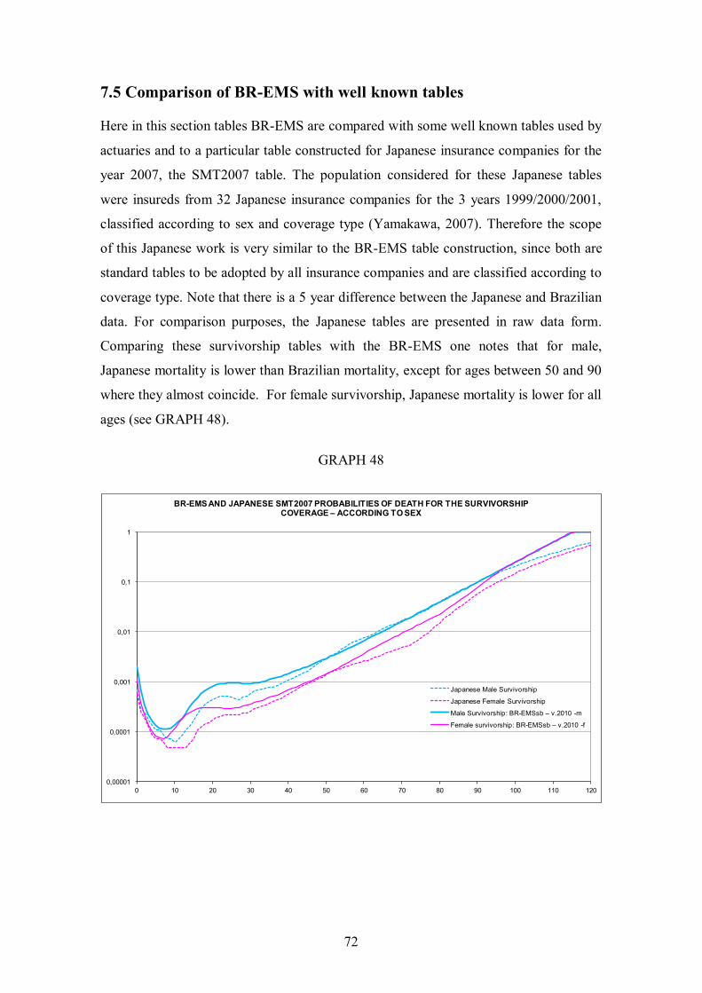
72

7.5 Comparison of BR-EMS with well known tables

Here in this section tables BR-EMS are compared with some well known tables used by

actuaries and to a particular table constructed for Japanese insurance companies for the

year 2007, the SMT2007 table. The population considered for these Japanese tables

were insureds from 32 Japanese insurance companies for the 3 years 1999/2000/2001,

classified according to sex and coverage type (Yamakawa, 2007). Therefore the scope

of this Japanese work is very similar to the BR-EMS table construction, since both are

standard tables to be adopted by all insurance companies and are classified according to

coverage type. Note that there is a 5 year difference between the Japanese and Brazilian

data. For comparison purposes, the Japanese tables are presented in raw data form.

Comparing these survivorship tables with the BR-EMS one notes that for male,

Japanese mortality is lower than Brazilian mortality, except for ages between 50 and 90

where they almost coincide. For female survivorship, Japanese mortality is lower for all

ages (see GRAPH 48).

GRAPH 48

0,00001

0,0001

0,001

0,01

0,1

1

0 10 20 30 40 50 60 70 80 90 100 110 120

BR-EMS AND JAPANESE SMT2007 PROBABILITIES OF DEATH FOR THE SURVIVORSHIP COVERAGE – ACCORDING TO SEX

Japanese Male Survivorship

Japanese Female Survivorship

Male Survivorship: BR-EMSsb – v.2010 -m

Female survivorship: BR-EMSsb – v.2010 -f

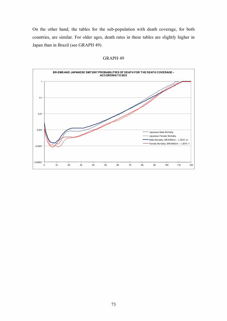
73

On the other hand, the tables for the sub-population with death coverage, for both

countries, are similar. For older ages, death rates in these tables are slightly higher in

Japan than in Brazil (see GRAPH 49).

GRAPH 49

0,00001

0,0001

0,001

0,01

0,1

1

0 10 20 30 40 50 60 70 80 90 100 110 120

BR-EMS AND JAPANESE SMT2007 PROBABILITIES OF DEATH FOR THE DEATH COVERAGE –ACCORDING TO SEX

Japanese Male Mortality

Japanese Female Mortality

Male Mortality: BR-EMSmt – v.2010 -m

Female Mortality: BR-EMSmt – v.2010 -f

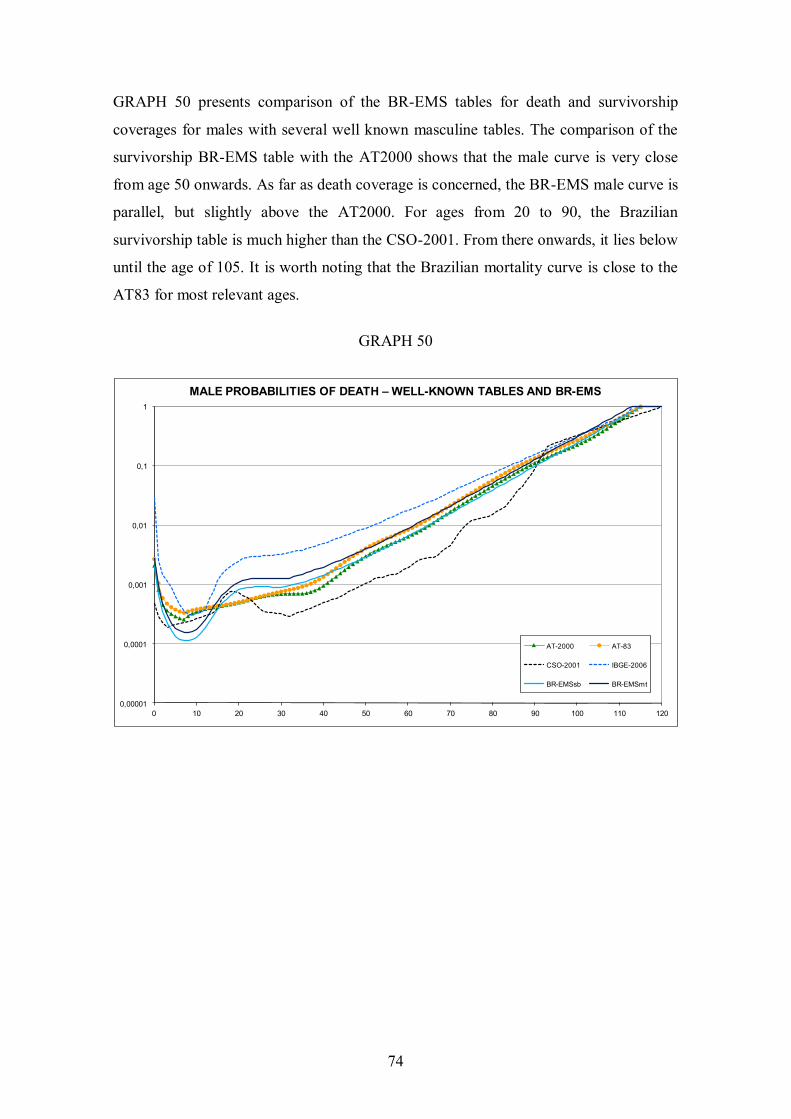
74

GRAPH 50 presents comparison of the BR-EMS tables for death and survivorship

coverages for males with several well known masculine tables. The comparison of the

survivorship BR-EMS table with the AT2000 shows that the male curve is very close

from age 50 onwards. As far as death coverage is concerned, the BR-EMS male curve is

parallel, but slightly above the AT2000. For ages from 20 to 90, the Brazilian

survivorship table is much higher than the CSO-2001. From there onwards, it lies below

until the age of 105. It is worth noting that the Brazilian mortality curve is close to the

AT83 for most relevant ages.

GRAPH 50

0,00001

0,0001

0,001

0,01

0,1

1

0 10 20 30 40 50 60 70 80 90 100 110 120

MALE PROBABILITIES OF DEATH – WELL-KNOWN TABLES AND BR-EMS

AT-2000 AT-83

CSO-2001 IBGE-2006

BR-EMSsb BR-EMSmt

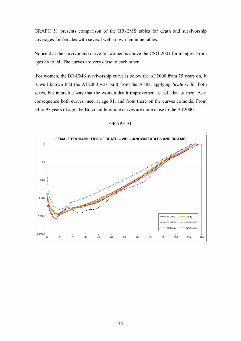
75

GRAPH 51 presents comparison of the BR-EMS tables for death and survivorship

coverages for females with several well known feminine tables.

Notice that the survivorship curve for women is above the CSO-2001 for all ages. From

ages 86 to 94. The curves are very close to each other.

For women, the BR-EMS survivorship curve is below the AT2000 from 75 years on. It

is well known that the AT2000 was built from the AT83, applying Scale G for both

sexes, but in such a way that the women death improvement is half that of men. As a

consequence both curves meet at age 91, and from there on the curves coincide. From

34 to 97 years of age, the Brazilian feminine curves are quite close to the AT2000.

GRAPH 51

0,00001

0,0001

0,001

0,01

0,1

1

0 10 20 30 40 50 60 70 80 90 100 110 120

FEMALE PROBABILITIES OF DEATH – WELL-KNOWN TABLES AND BR-EMS

AT-2000 AT-83

CSO-2001 IBGE-2006

BR-EMSsb BR-EMSmt

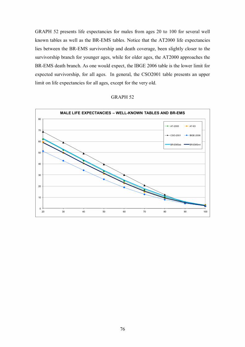
76

GRAPH 52 presents life expectancies for males from ages 20 to 100 for several well

known tables as well as the BR-EMS tables. Notice that the AT2000 life expectancies

lies between the BR-EMS survivorship and death coverage, been slightly closer to the

survivorship branch for younger ages, while for older ages, the AT2000 approaches the

BR-EMS death branch. As one would expect, the IBGE 2006 table is the lower limit for

expected survivorship, for all ages. In general, the CSO2001 table presents an upper

limit on life expectancies for all ages, except for the very old.

GRAPH 52

0

10

20

30

40

50

60

70

80

20 30 40 50 60 70 80 90 100

MALE LIFE EXPECTANCIES – WELL-KNOWN TABLES AND BR-EMS

AT-2000 AT-83

CSO-2001 IBGE-2006

BR-EMSsb BR-EMSmt

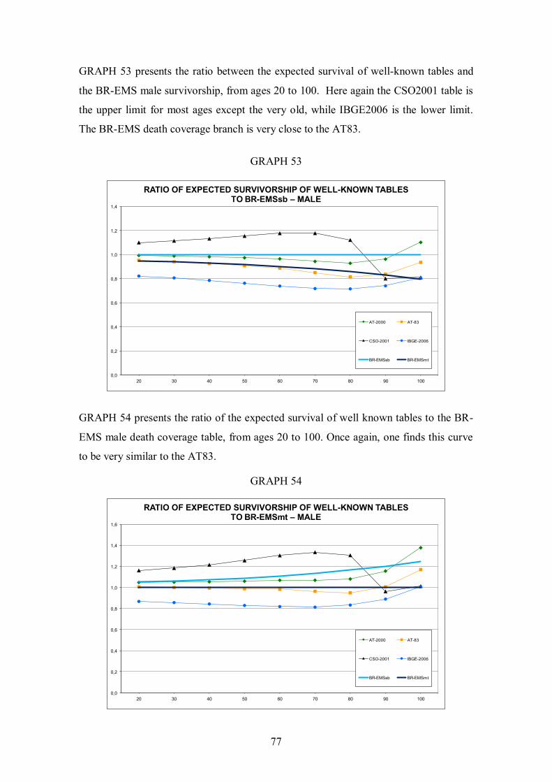
77

GRAPH 53 presents the ratio between the expected survival of well-known tables and

the BR-EMS male survivorship, from ages 20 to 100. Here again the CSO2001 table is

the upper limit for most ages except the very old, while IBGE2006 is the lower limit.

The BR-EMS death coverage branch is very close to the AT83.

GRAPH 53

0,0

0,2

0,4

0,6

0,8

1,0

1,2

1,4

20 30 40 50 60 70 80 90 100

RATIO OF EXPECTED SURVIVORSHIP OF WELL-KNOWN TABLES TO BR-EMSsb – MALE

AT-2000 AT-83

CSO-2001 IBGE-2006

BR-EMSsb BR-EMSmt

GRAPH 54 presents the ratio of the expected survival of well known tables to the BR-

EMS male death coverage table, from ages 20 to 100. Once again, one finds this curve

to be very similar to the AT83.

GRAPH 54

0,0

0,2

0,4

0,6

0,8

1,0

1,2

1,4

1,6

20 30 40 50 60 70 80 90 100

RATIO OF EXPECTED SURVIVORSHIP OF WELL-KNOWN TABLES TO BR-EMSmt – MALE

AT-2000 AT-83

CSO-2001 IBGE-2006

BR-EMSsb BR-EMSmt

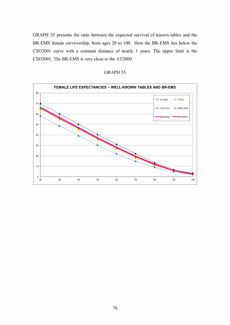
78

GRAPH 55 presents the ratio between the expected survival of known tables and the

BR-EMS female survivorship, from ages 20 to 100. Here the BR-EMS lies below the

CSO2001 curve with a constant distance of nearly 3 years. The upper limit is the

CSO2001. The BR-EMS is very close to the AT2000.

GRAPH 55

0

10

20

30

40

50

60

70

80

20 30 40 50 60 70 80 90 100

FEMALE LIFE EXPECTANCIES – WELL-KNOWN TABLES AND BR-EMS

AT-2000 AT-83

CSO-2001 IBGE-2006

BR-EMSsb BR-EMSmt

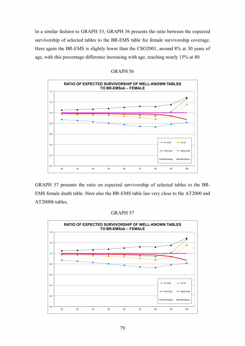
79

In a similar fashion to GRAPH 53, GRAPH 56 presents the ratio between the expected

survivorship of selected tables to the BR-EMS table for female survivorship coverage.

Here again the BR-EMS is slightly lower than the CSO2001, around 8% at 30 years of

age, with this percentage difference increasing with age, reaching nearly 15% at 80.

GRAPH 56

0,0

0,2

0,4

0,6

0,8

1,0

1,2

1,4

20 30 40 50 60 70 80 90 100

RATIO OF EXPECTED SURVIVORSHIP OF WELL-KNOWN TABLES TO BR-EMSsb – FEMALE

AT-2000 AT-83

CSO-2001 IBGE-2006

BR-EMSsb BR-EMSmt

GRAPH 57 presents the ratio on expected survivorship of selected tables to the BR-

EMS female death table. Here also the BR-EMS table lies very close to the AT2000 and

AT2000b tables.

GRAPH 57

0,0

0,2

0,4

0,6

0,8

1,0

1,2

1,4

20 30 40 50 60 70 80 90 100

RATIO OF EXPECTED SURVIVORSHIP OF WELL-KNOWN TABLES TO BR-EMSsb – FEMALE

AT-2000 AT-83

CSO-2001 IBGE-2006

BR-EMSsb BR-EMSmt

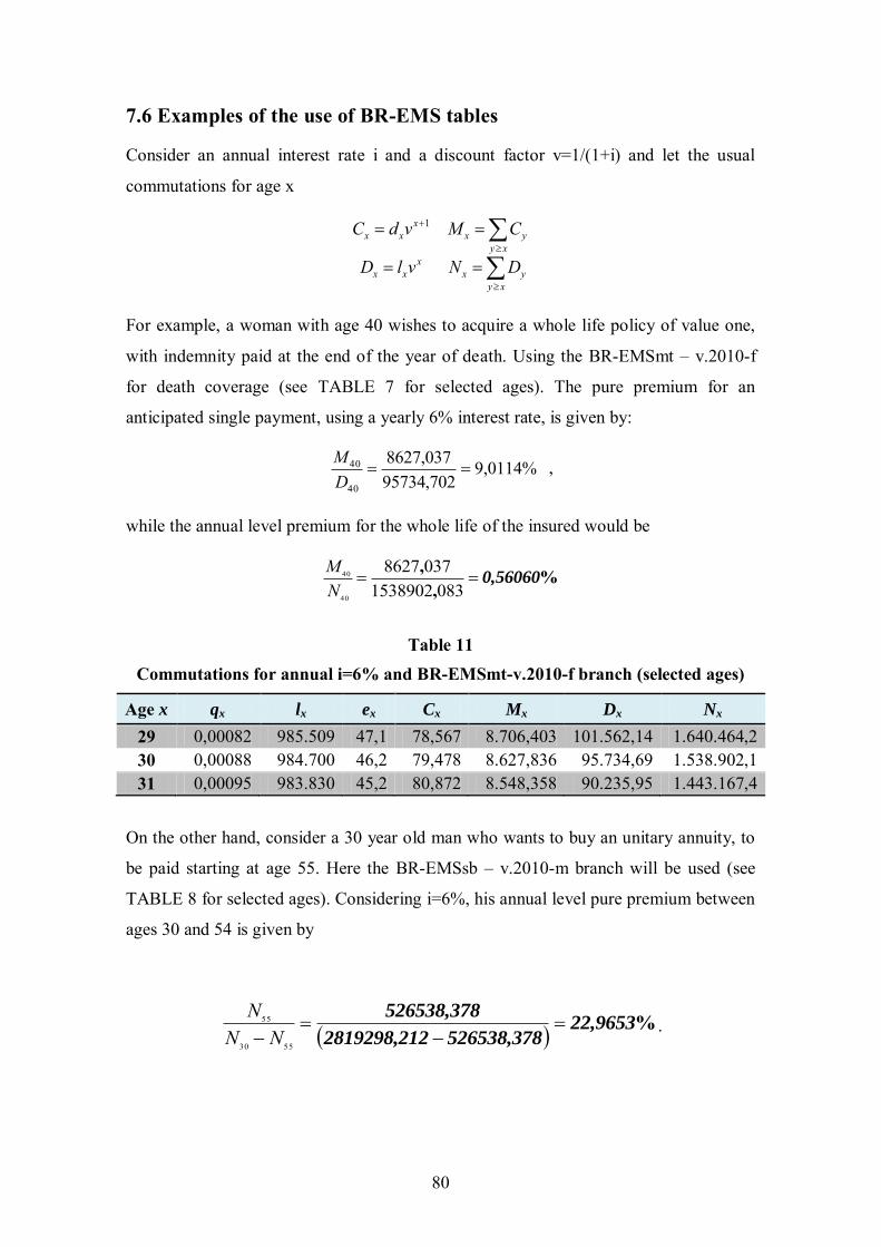
80

7.6 Examples of the use of BR-EMS tables

Consider an annual interest rate i and a discount factor v=1/(1+i) and let the usual

commutations for age x

xyyx

xxx

xyyx

xxx

DNvlD

CMvdC 1

For example, a woman with age 40 wishes to acquire a whole life policy of value one,

with indemnity paid at the end of the year of death. Using the BR-EMSmt – v.2010-f

for death coverage (see TABLE 7 for selected ages). The pure premium for an

anticipated single payment, using a yearly 6% interest rate, is given by:

%9,0114702,95734

037,8627

40

40 DM

,

while the annual level premium for the whole life of the insured would be

%,

,0,56060

08315389020378627

40

40

NM

Table 11 Commutations for annual i=6% and BR-EMSmt-v.2010-f branch (selected ages)

Age x qx lx ex Cx Mx Dx Nx

29 0,00082 985.509 47,1 78,567 8.706,403 101.562,14 1.640.464,2 30 0,00088 984.700 46,2 79,478 8.627,836 95.734,69 1.538.902,1 31 0,00095 983.830 45,2 80,872 8.548,358 90.235,95 1.443.167,4

On the other hand, consider a 30 year old man who wants to buy an unitary annuity, to

be paid starting at age 55. Here the BR-EMSsb – v.2010-m branch will be used (see

TABLE 8 for selected ages). Considering i=6%, his annual level pure premium between

ages 30 and 54 is given by

%22,9653

526538,37822819298,21

526538,378

5530

55

NNN

.

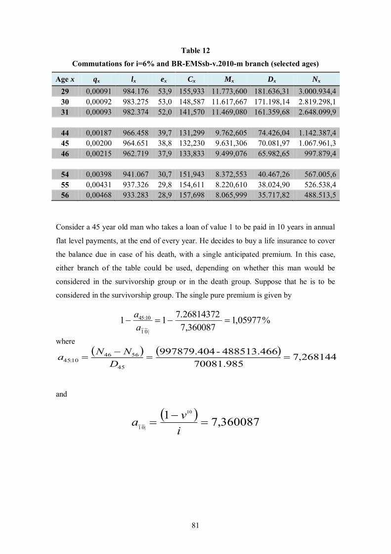
81

Table 12

Commutations for i=6% and BR-EMSsb-v.2010-m branch (selected ages)

Age x qx lx ex Cx Mx Dx Nx

29 0,00091 984.176 53,9 155,933 11.773,600 181.636,31 3.000.934,4 30 0,00092 983.275 53,0 148,587 11.617,667 171.198,14 2.819.298,1 31 0,00093 982.374 52,0 141,570 11.469,080 161.359,68 2.648.099,9

44 0,00187 966.458 39,7 131,299 9.762,605 74.426,04 1.142.387,4 45 0,00200 964.651 38,8 132,230 9.631,306 70.081,97 1.067.961,3 46 0,00215 962.719 37,9 133,833 9.499,076 65.982,65 997.879,4

54 0,00398 941.067 30,7 151,943 8.372,553 40.467,26 567.005,6 55 0,00431 937.326 29,8 154,611 8.220,610 38.024,90 526.538,4 56 0,00468 933.283 28,9 157,698 8.065,999 35.717,82 488.513,5

Consider a 45 year old man who takes a loan of value 1 to be paid in 10 years in annual

flat level payments, at the end of every year. He decides to buy a life insurance to cover

the balance due in case of his death, with a single anticipated premium. In this case,

either branch of the table could be used, depending on whether this man would be

considered in the survivorship group or in the death group. Suppose that he is to be

considered in the survivorship group. The single pure premium is given by

%05977,1360087,7

7.2681437211|01

10:45 aa

where

268144,770081.985

488513.466-997879.40445

564610:45

DNNa

and

360087,71 10

|01

iva

82

REFERENCES

ABDOUG, B.; GHOUDI, K.; and KHOUDRAJI, A.. Non parametric estimation of the

limit dependence function of multivariate extremes. Extremes, 2(3):245-268, 1999.

ANDREEV, Kirill F. and VAUPEL, James W.. Patterns of Mortality Improvement over

Age and Time in Developed Countries: Estimation, Presentation and Implications for

Mortality Forecasting. Web February 12, 2005

AON CONSULTING. Implications of the adoption of the 2001 CSO: a research report

from Aon Insurance Consulting Service, September, 2002.

BALKEMA, A.A.; and de HAAN, L. Residual life time at great age. Annals of

Probability, 2:792{804, 1974.

BARBI, Elisabetta. Assessing the rate of ageing of the human population, MPIDR

WORKING PAPER WP 2003-008, MARCH 2003

BELTRÃO, Kaizô Iwakami; SUGAHARA, Sonoe. Taxas de Mortalidade no Setor de

Seguros – 1998-2000. Estimativas e Comparações com Tábuas de Mercado. Rio de

Janeiro, Funenseg 250 pp, 2005.

BELTRÃO, Kaizô Iwakami; SUGAHARA, Sonoe. Tábua de mortalidade para os

funcionários públicos civis federais do poder executivo por sexo e escolaridade:

comparação com tábuas do mercado. TD 3, ENCE/IBGE, Rio de Janeiro, de 2002b.

BELTRÃO, Kaizô Iwakami; SUGAHARA, Sonoe. Mortality Rates in the Brazilian

Insurance Market: a Comparison. Brazilian Journal of Probability and Statistics, 19,2,

December 2005.

BENNETT, Neil G; HORIUCHI, Shiro. Estimating the completeness of death

registration in a closed population: current items. Population Index, Princeton, NJ,

USA, pp. 207-222, 1981.

BLOOMFIELD, D. S. F. & HABERMAN, S. Graduation: some experiments with

kernel methods. JIA 114 (1987) 339-369

BONGAARTS, John & FEENEY, Grifth. How long do we live? Population Council.

Policy Research Division, Working Paper No. 156, 2002.

BONGAARTS, John & FEENEY, Grifth. Estimating Mean Lifetime. Population

Council. Policy Research Division, Working Paper No. 179, 2003.

83

BOWERS, N. L.; GERBER, H.U.; HICKMAN, J. C.; and NESBIT, C. J. Actuarial

Mathematics. Society of Actuaries, Itasca, Illinois, 1986.

BRASS, William. Methods for estimating fertility and mortality from limited and

defective data. Chapell Hill, North Carolina, Carolina Population Center, Laboratories

for Population Studies, 1975.

BRIAN, Eric; ROHRBASSER, Jean-Marc; THÉRÉ, Christine; et VÉRON, Jacques. La

duree de vie: Histoire et calcul - especulations sur la vie humaine et crise financiere a

la fin du XVIII-eme siecle. l’INED - DOCUMENTS DE TRAVAIL, 109, 2002.

BRILLINGER, D.R. A justification of some common laws of mortality, Transactions of

the Society of Actuaries, 116-126, 1961.

CARRIERE, Jacques F.. Parametric models for life tables. Transactions of Society of

Actuaries, 1992 vol. 44.

CARRIERE, Jacques F.. A Select and Ultimate Parametric Model. Transactions of

society of Actuaries, 1994 vol. 46.

COALE, Ansley J. & Demeny Paul, Regional Model Life Tables and Stable Population,

Princeton UP, Princeton, NJ, 1966.

Continuous Mortality Investigation/Mortality Committee. The Graduation of the CMI

1999-2002 Mortality Experience: Feedback on Working Paper 8 and Proposed Assured

Lives Graduations. CMI Working Paper 12, April 2005.

_________________________________. Projecting future mortality: Towards a

proposal for a stochastic methodology. CMI Working Paper 15, July 2005.

_________________________________. The Graduation of the CMI 1999-2002

Mortality Experience: Proposed Annuitant and Pensioner Graduations. CMI Working

Paper 16, September 2005.

_________________________________. The Graduation of the CMI 1999-2002

Mortality Experience: Final “00” Series Mortality Tables – Assured Lives. CMI

Working Paper 21, July 2006.

_________________________________. The Graduation of the CMI 1999-2002

Mortality Experience: Final “00” Series Mortality Tables – Annuitants and Pensioners.

CMI Working Paper 22, July 2006.

84

_________________________________. Stochastic projection methodologies: Lee-

Carter model features, example results and implications. CMI Working Paper 25, April

2007.

_________________________________. Extensions to Younger Ages of the “00”

Series Pensioner Tables of mortality. CMI Working Paper 26, April 2007.

_________________________________. The “library” of Mortality Projections. CMI

Working Paper 27, July 2007.

COPAS, J.B. & HABERMAN, M. A. (1983). Non-parametric graduation using kernel

methods, Journal of the Institute of Actuaries, 110, 135-156.

COURBAGE, Youssef; FARGUES, Philippe. A method for deriving mortality

estimates from incomplete vital statistics. Population Studies, 33, 1, 1979.

CURRIE, Iain; KIRKBY, James; DURBAN, Maria; and EILERS, Paul. Smooth Lee-

Carter Models and Beyond. International Centre for Mathematical Sciences, Edinburgh,

September 2004.

HELIGMAN, Larry; POLLARD, J. H.. The age pattern of mortality. Readings in

Population Research Methodology, v.2, pp. 97-104, 1980.

JOSEPH, A.W. The Whittaker-Henderson method of graduation, Journal of the Institute

of Actuaries, 99-114, 1952.

KIMELDORF, G. S. e JONES, D. A. Bayesian graduation. Transactions of Society of

Actuaries, v. 19, 1967, p 66-112.

KOSTAKI, A. & PANOUSIS, V. Expanding an abridged life table, Demographic

Research, vol.5, article 1, 2001.

LAUDERDALE Diane S. & KESTENBAUM Bert, Mortality rates of elderly Asian

American populations, Demography, 39,3, August 2002.

LEDERMANN, S. & BREAS, Jean. “Les dimensions de la mortalité”, Population, 14,

4, 1959.

LEE, Ronald D.; CARTER, Lawrence R. Modeling and forecasting the time series of

US mortality. Journal of the American Statistical Association, 87: pp.659-71, 1992.

LEVY, A. & ZACS, A. Dynamical Life Tables, Technion, IIT, Haifa, 2002.

85

NAVATHE, S., ELMASRI, R., “Fundamentals of Database Systems”, Addison

Wesley; 6th edition; 2011

ROLAND, Rau; SOROKO, Eugeny; JASILIONIS, Domantas; VAUPEL, James W. 10

years after Kannisto: further evidence for mortality decline at advanced ages in

developed countries, MPIDR WORKING PAPER WP 2006-033 October 2006.

RENSHAW, A. E. e HABERMAN, S. Modelling for mortality reduction factors.

Actuarial Research Paper, v. 127. London: City University, 2000.

ROSENWAIKE Ira & STONE, Leslie F. Verification of the ages of super centenarians

in the United States: results of a matching study, Demography, vol. 40, pp.727-739,

2003.

SEAL, H.L. Tests Of Mortality Table Graduation, Journal Of The Institute Of

Actuaries, 5-67, 1953.

TUKEY, JOHN W (1977). Exploratory Data Analysis. Addison-Wesley.

UNITED NATIONS, Manual X: Indirect techniques for demographic estimation, New

York, 1983.

UNITED NATIONS, Model Life Tables for Developing Countries, New York, 1983.

VALLIN, J., MESLÉ, F.; Trends in mortality and differential mortality, Population

studies No. 36, Council of Europe Publishing, ISBN 92-871-4725-6, December 2001; In

www.coe.int/t/e/social_cohesion/population/N%C2%B036_Trends_in_mortality.pdf

VAUPEL, James W. et al. Biodemographic Trajectories of Longevity. Science, vol.

280: pp.855-60, 1998.

VERRALL, R. (1996). A Unified Framework For Graduation, Actuarial Research Paper

91, CITY University, London, UK.

WACHETER, Kenneth W.; FINCH, Caleh E. eds. Between Zeus and the salmon – The

biodemography of longevity. National Academy Press, Washington D.C., 1997.

YAMAKAWA, Tatsuhiro. The standard mortality table 2007. Tokyo: Institute of

Actuaries of Japan, 2007. In www.actuaries.jp/eaac14th/pdf/session/06_2P_Yamakawa

Tatsuhiro_18Revised.pdf