Embed Size (px)
Citation preview

Dipartimento di Scienze Statistiche
Sezione di Statistica Economica ed Econometria
Elisa Fusco Bernardo Maggi
Bank financial world crisis: inefficienciesand responsibilities
DSS Empirical Economics and EconometricsWorking Papers Series
DSS-E3 WP 2016/2

Dipartimento di Scienze StatisticheSezione di Statistica Economica ed Econometria
“Sapienza” Università di RomaP.le A. Moro 5 – 00185 Roma - Italia
http://www.dss.uniroma1.it
Bank Financial world crisis:Inefficiencies and Responsibilities
Elisa Fuscoa, Bernardo Maggi b,∗
aUniversity of Rome La SapienzabDepartment of Statistical Sciences, University of Rome La Sapienza, Faculty of
Engineering, Informatics and Statistics
Abstract
In light of the recent financial world crisis, is crucial to investigate into theresponsibilities of the main actors in the credit sectors, i.e. banks and local gov-ernments.
In this framework, we propose a methodology able to analyze the quality ofthe problem loans adopted by banks, their level of efficiency in the risk man-agement strategies and the governments policy action in the supervision of thelocal banking system. Our approach is based on the introduction of the “Nonperforming Loans” variable as an undesirable output in an output distance func-tion (as stochastic frontier) in order to estimate the efficiency of the bank andcalculate the shadow price of the NPLs (not normally observable) per each year,bank and country. Then we compare the management of the NPLs and theirprice across geographic areas and bank dimension over time in order to map theresponsibilities and to draw some policy implications.
From an econometric point of view, we -to our knowledge- for first adopt thesemi-nonparametric Fourier specification which, among the functional-flexible-form alternatives, is capable to guarantee the convergence of the estimated pa-rameters and the related X-efficiency to the true ones.
Keywords: Commercial bank, Financial world crisis, Non performing loans,Efficiency, Flexible forms, Distance functionJEL classification: G21, D24, C33, C51, L23.
∗Corresponding author.Email addresses: [email protected] (Elisa Fusco ),
[email protected] (Bernardo Maggi )
1. Introduction
Till recently, most part of the literature of banking systems efficiency ne-glected the question of problem loans. Under the influence of the 2008-9 cri-sis, such a question started having growing consideration. Berger and DeYoung(1997) pioneered this field trying to face the study of the relations between prob-lem loans and efficiency by means of the Granger-causality method, Hughes andMester (1993) considered problem loans inside the frontier function. However,both of the attempts are not satisfactory because, the former is a mere statisticaltool based on the VAR methodology and so deprived from an economic inter-pretation of causality, the latter is incoherent since an increase of efficiency maybe due simply by increasing number of regressors. Only at the beginning ofthe first decade of 20s with the works of Pastor (2002) and Pastor and Serrano(2005) the question under consideration has been addressed properly with a nonparametric approach, which is of less powerful insight from the modelizationpoint of view. Pastor and Serrano (2006) adopted a parametric approach but didnot find a functional relationship between stochastic frontier and non performingloans (NPLs) and focused their investigation on the connection between NPLsand X-efficiency. Maggi and Guida (2011) addressed this point by consideringan indirect function linking NPLs with stochastic frontier.
With the present work we go further by inserting directly the NPLs variablein the stochastic frontier as a negative output, taking advantage of the fact thatour definition of efficiency relies on the concept of the distance function. In sucha way we are capable to asses on the quality of the problem loans adopted bybanks and on their responsibility in the risk management. The former question isaddressed by calculating the price of non performing loans per each year, bankand country considered in our dataset, the latter by comparing the management- in terms of variance analysis - of NPLs and their price across geographic areasand bank dimension over time. In doing so we provide a methodology whichallows from one hand to alert in advance on an incumbent state of crisis and, fromthe other hand to evaluate the responsibility to be imputed to the main actors inthe credit sectors, i.e. banks and local governments. Furthermore, an economicpolicy in terms of regulatory activities focused on the NPLs price comes outnaturally as an implication of the analysis implemented. In fact, notably, theNPLs price is unknown and therefore not normally observable. Instead, ourmethodology allows to calculate it from the first order conditions underlyingthe estimation performed. Indeed, also in Maggi and Guida (2011) there is thepossibility to evaluate a similar indicator. However, from the cost function thereconsidered, the marginal cost calculated cannot be assumed as a price-quality
2
indicator in that this would have been possible only with perfect competitionwhich is not the case for credit market. Moreover, that methodology passesthrough the definition of a density function which inevitably involves a degreeof arbitrariness in its form of definition. From an econometric point of view, we-to our knowledge- for first adopt the semi-nonparametric Fourier specificationwhich, among the functional-flexible-form alternatives, is capable to guaranteethe convergence of the estimated parameters and the related X-efficiency to thetrue ones (Gallant (1981), Berger et al. (1997)).
Then our goals consist in: 1) finding a map of the responsibilities of the lastfinancial crisis, 2) finding a road to regulate the risk in the credit market, 3) alert-ing the crisis period, 4) providing a rigorous method to calculate efficiency incase of a production function with undesired outputs. In order to cope with ex-igency of monitoring the credit sector, for what said above, our prime necessityis to calculate the shadow-price applied to NPLs. Hence, in the second sectionwe define the theoretical framework of the model, where the optimizing behav-ior of the banks in charging prices is described. In the third section we describeour dataset and variables. In the fourth section, we derive, specifically for thenon performing loans the analytical expression of such a price and the analyt-ical form used in the empirical analysis. In the fifth section, we estimate thedistance-revenue function. In the sixth section, we obtain the evaluation of theX-efficiency and the distribution of the NPLs price, which let us detect the out-coming responsibilities and omissions in the monitoring processes relatively tothe last financial world crisis. The seventh section draws some comments on themain results with the policy implications. The eight section concludes.
2. Theoretical model
In this section we present the model for the determination of banks outputsprices. We intend to derive the X-inefficiency and a closed form solution for priceof problem loans conceived as a negative output. Such a closed form will be usedfor the estimation in the next section. The representative commercial bank uses apositive vector of N inputs, denoted by x= (x1, ...,xN) , x∈RN
+ to produce a pos-itive vector of M outputs, denoted by u = (u1, ...,uM) , u ∈ RM
+ . The productiontechnology of the bank can be defined by the output set, P(x) that can be pro-duced by means of the input vector x, i.e., P(x) =
{u ∈ RM
+ : x can produce u}
.It is also assumed that technology satisfies the usual axioms initially proposed byShephard (1970), which allow to define the distance function -in terms of output-as the reciprocal of the maximum radial expansion of a given output vector pro-portional to the maximum output attainable. In such a way the resulting output
3
vector remains within P(x), being attainable using the available resources andtechnology. The output distance can be formally defined as 1:
Do(x,u) = in f{
θ :(u
θ
)∈ P(x)
}(1)
where Do(x,u) is the distance from the banks output set to the frontier, and θ ∈[0,1] is the corresponding level of efficiency. The output distance function seeksthe largest proportional increase in the observed output vector u provided thatthe expanded vector ( u
θ)) is still an element of the original output set (Fare and
Primont (1995)). Such an expression defines the weak disposability of outputsand therefore the inefficiency, which could explain, in our context, the presenceof NPLs (undesirable outputs) that banks generate in their production processes,and that cannot freely eliminate either because it would require a greater useof inputs, and/or because resources would have to be diverted from marketableproduction.
In effect, by considering the NPLs as an output of a production process, otherthan to give the advantage of deriving the correspondent price, eliminates the em-pirical complications that would have occurred using a cost function approach.In fact, in this case a simultaneity problem would have been arisen between inef-ficiency and therefore costs- and NPLs considered as an explicative variable. Ourapproach exploits the duality of maximum revenue problem, expressed in termsof distance function (1), where the correspondence between the primal and thedual problems relies on efficiency and output prices. Furthermore, such an ap-proach allows to define inefficiency as a function of outputs and prices, includedthat one of NPLs, on which the empirical analysis is focused. More specifically,undesirable outputs, such as NPLs, have non-positive shadow prices that maybe obtained empirically by exploiting the above mentioned duality. Now we setprimal and revenue function problems in order to find the two correspondingshadow prices vectors in natural numbers and normalized for the revenue func-tion, respectively. Then, we find the NPLs price in natural numbers from therevenue function.
Denoting by r = (r1, ...,rM) the output prices-vector, and assuming that rm 6=0, the revenue function in terms of the distance function may be expressed as:
maxR(x,r) = maxu
{r′u : u ∈ P(x)
}(2)
1This expression is equivalent to the reciprocal of the output oriented efficiency measure ofFarrell (Farrell (1957) and Fare and Knox Lovell (1978)).
4
If the parent technology has convex output sets P(x), for all x ∈ RN+ , then
one can prove (see Shephard (1970) or Fare (1988)) that the following dualityholds:
R(x,r) = supu
{r′u : Do(x,u)≤ 1
}Do(x,u) = sup
r
{r′u : R(x,r)≤ 1
} (3)
that is, the revenue function may be obtained by maximizing revenue with re-spect to outputs compatibly with the output distance function, which in its turnmay be obtained by maximizing the actual revenue function with respect to out-put prices (normalized for the maximum revenue) compatibly with the attainablerevenue out of the maximum one. Then, assuming that the revenue and distancefunctions are both differentiable, a Lagrange problem can be set up to maximizerevenue:
maxu
Λ = r′u+λ (Do(x,u)−1) (4)
and first order conditions with respect to outputs yield the relationship (Fare andPrimont (1995)):
r =−λOuDo(x,u) (5)
At the optimum, in force of the homogeneity of degree 1 of Do(x,u) (see Ja-cobsen (1972)), the negative of the Lagrange multiplier equals the revenue func-tion, i.e., −λ = Λ = R(x,r). Thus, we may write (5) in terms of the followingsystem of equations:
r = R(x,r)OuDo(x,u) (6)
Now by means of the second part of the duality theorem (3), we obtain that:
Do(x,u) = r∗(x,u)u (7)
where r∗(x,u) represents the output price vector that maximises revenue.Applying Shephards dual lemma to expression (7), yields:
OuDo(x,u) = r∗(x,u) (8)
which, combined with (6), leads to:
r = R(x,r)r∗(x,u) (9)5
where, r∗(x,u) is obtained from the gradient of the distance function, andrepresents revenue-deflated output prices. The main difficulty that arises in orderto obtain absolute shadow prices from expression (9) is due to the dependenceof the revenue function R(x,r) on r, that is precisely the vector of shadow priceswe are seeking for.
Therefore, in order to obtain R(x,r) we assume that ”The observed price ofan output m, ro
m , equals its absolute shadow price rm”, which allows to obtainthe maximum revenue as:
R =ro
mr∗m(x,u)
(10)
which may be used to calculate the absolute shadow prices of the remainingoutputs from its deflated shadow prices r∗. Denoting by rm′ the absolute shadowprices for outputs other than m, we get:
rm′ = R · r∗m′(x,u) = R · ∂Do(x,u)∂um′
= rom ·
∂Do(x,u)/∂um′
∂Do(x,u)/∂um(11)
3. Variables and data
Data are from Bankscope and are referred to 517 Commercial Banks in Eu-rope and 2404 in the U.S., the sample period is 2000-2008. Europe includes theEuro system plus UK, Sweden, Norway and Turkey. The list of countries consid-ered is reported in the following Tables 1 and 2. The large database used enablesto asses very specifically both on the responsibilities of the single country policyand legislation and on the bank discipline during the last financial crisis.
The specification we adopt for the distance function is the production ap-proach with three outputs and two inputs. Among desirable outputs we considerdeposits (u1), loans (u2) and services (u3), NPL (u4) is the undesirable output andinputs are capital (x1) and labor (x2). Deposits are regarded as an output, ratherthan an input, for the diminishing importance of the corresponding interest ratestill in the commercial banking system. All variables are expressed in nominal(dollar) values at constant prices (year 2000). The labor price is calculated astotal personnel cost divided by the number of employees. Fixed assets have beentransformed from the historical cost evaluation of balance sheet (InternationalAccounting Standards 16) to current cost. As for capital price we estimate thefollowing indirect function where the total capital is proxied2:
2We tried also direct functions both linear and logarithmic and other indirect functions withless qualitative results available upon request.
6

log(CapitalCostkt) =K
∑k=1
dpck · log(pck0)+β1log(
At +Lt
2
)+ εkt (12)
for k = 1, ...,K, t = 2000, ...,2008where At stands for total assets, Lt for total liabilities, pck are estimated coeffi-cients of the dummy variables dpck representing the capital price for each branch
and β1log(
At+Lt2
)is the proxied total capital.
The services variable is constructed as the total value of ”net” services.
Importantly, NPLs have different definitions across European countries andin the U.S.. In particular, the U.S. definition includes only the protested creditswhilst a more prudential definition is adopted in Europe where are also consid-ered the uncertain loans. We may now calculate a first indicator of the bankingsystem risk consisting in the empirical NPLs failure probability for loans givenby NPLs out of loans and reported in Figure 1.
Below are shown the descriptive statistics. We consider the mean and thestandard deviation of the variables used in the estimation.
Table 1: Descriptive statistics: Europe (Time average data are expressed in millions of Dollars)
NonCountry Statistics Deposits Loans Services Capital Labour Performing
(u1) (u2) (u3) (x1) (x2) loans (u4)Austria Mean 1747,04 1213,82 18,32 5985,93 267 12,09
St. Dev. 5977,25 4553,54 32,11 18095,67 797 27,11Belgium Mean 2031,03 1306,25 20,79 4488,13 404 17,84
St. Dev. 2170,53 1677,11 26,58 4974,75 407 15,84Denmark Mean 4661,29 4252,55 47,77 15587,65 885 27,34
St. Dev. 17543,28 14334,46 151,75 55413,08 2459 60,31Finland Mean 21048,81 14555,98 238,64 67574,18 3183 91,98
St. Dev. 23227,00 15318,52 294,19 87932,30 3372 68,33France Mean 13656,28 6885,30 164,02 37467,77 1777 37,99
St. Dev. 68586,04 30746,82 799,17 205861,30 6327 88,48Germany Mean 8495,53 5686,36 64,33 21259,51 815 30,50
St. Dev. 43770,04 25874,97 331,86 107016,10 3456 81,58Great Britain Mean 1425,02 661,53 18,11 3747,84 134 9,62
St. Dev. 3006,67 1646,89 41,26 9392,71 209 14,44Greece Mean 20988,58 14953,53 225,88 47050,90 5307 95,79
St. Dev. 19250,46 13110,13 247,78 43570,73 4192 61,60Ireland Mean 1628,32 876,27 4,16 11277,91 28 14,63
St. Dev. 1351,37 752,11 13,56 18714,80 24 9,34Italy Mean 9368,70 8047,37 151,08 29230,47 2156 51,09
St. Dev. 25245,42 21729,86 405,87 83840,79 5555 76,63Luxembourg Mean 6482,70 1791,80 51,02 14633,63 253 21,08
St. Dev. 9543,99 2645,64 86,90 20937,75 429 21,58Continued on Next Page. 7
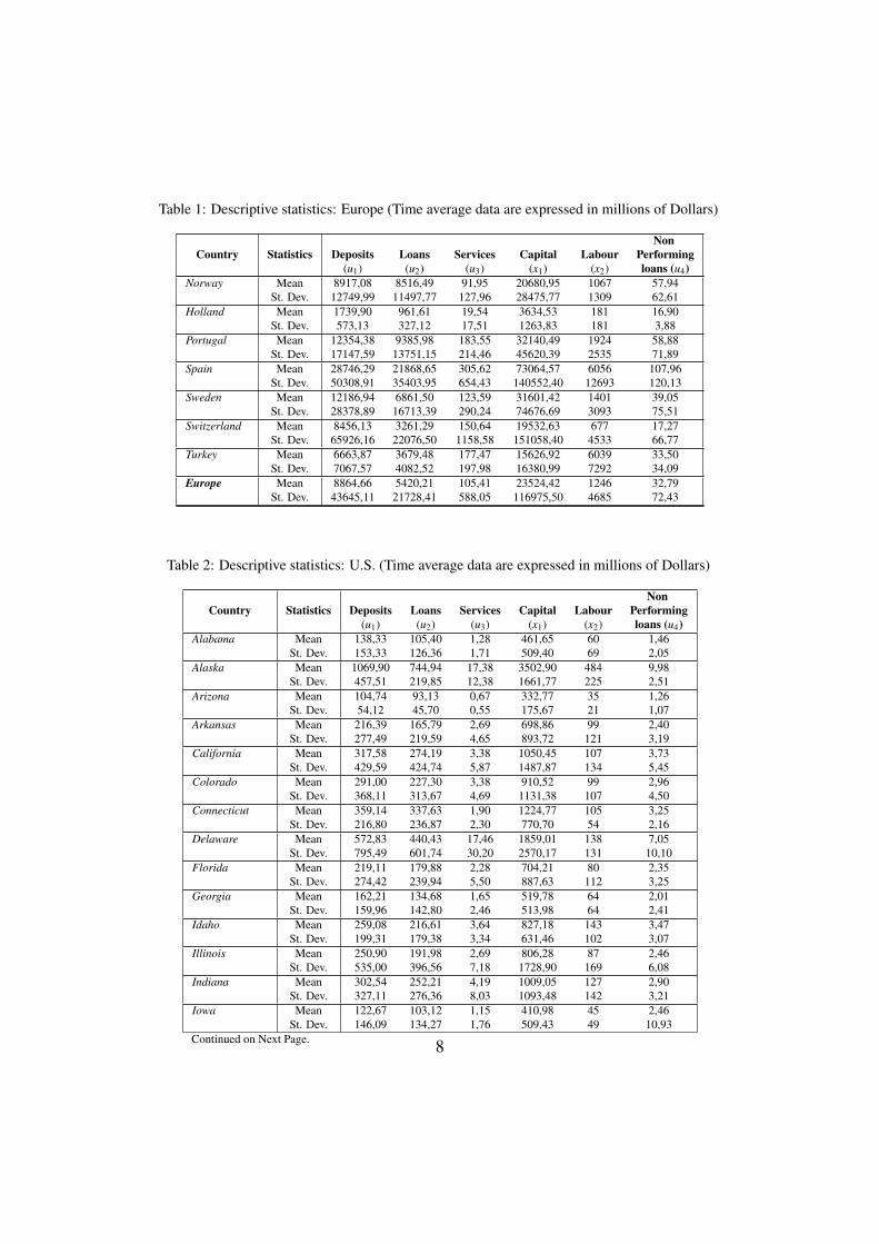
Table 1: Descriptive statistics: Europe (Time average data are expressed in millions of Dollars)
NonCountry Statistics Deposits Loans Services Capital Labour Performing
(u1) (u2) (u3) (x1) (x2) loans (u4)Norway Mean 8917,08 8516,49 91,95 20680,95 1067 57,94
St. Dev. 12749,99 11497,77 127,96 28475,77 1309 62,61Holland Mean 1739,90 961,61 19,54 3634,53 181 16,90
St. Dev. 573,13 327,12 17,51 1263,83 181 3,88Portugal Mean 12354,38 9385,98 183,55 32140,49 1924 58,88
St. Dev. 17147,59 13751,15 214,46 45620,39 2535 71,89Spain Mean 28746,29 21868,65 305,62 73064,57 6056 107,96
St. Dev. 50308,91 35403,95 654,43 140552,40 12693 120,13Sweden Mean 12186,94 6861,50 123,59 31601,42 1401 39,05
St. Dev. 28378,89 16713,39 290,24 74676,69 3093 75,51Switzerland Mean 8456,13 3261,29 150,64 19532,63 677 17,27
St. Dev. 65926,16 22076,50 1158,58 151058,40 4533 66,77Turkey Mean 6663,87 3679,48 177,47 15626,92 6039 33,50
St. Dev. 7067,57 4082,52 197,98 16380,99 7292 34,09Europe Mean 8864,66 5420,21 105,41 23524,42 1246 32,79
St. Dev. 43645,11 21728,41 588,05 116975,50 4685 72,43
Table 2: Descriptive statistics: U.S. (Time average data are expressed in millions of Dollars)
NonCountry Statistics Deposits Loans Services Capital Labour Performing
(u1) (u2) (u3) (x1) (x2) loans (u4)Alabama Mean 138,33 105,40 1,28 461,65 60 1,46
St. Dev. 153,33 126,36 1,71 509,40 69 2,05Alaska Mean 1069,90 744,94 17,38 3502,90 484 9,98
St. Dev. 457,51 219,85 12,38 1661,77 225 2,51Arizona Mean 104,74 93,13 0,67 332,77 35 1,26
St. Dev. 54,12 45,70 0,55 175,67 21 1,07Arkansas Mean 216,39 165,79 2,69 698,86 99 2,40
St. Dev. 277,49 219,59 4,65 893,72 121 3,19California Mean 317,58 274,19 3,38 1050,45 107 3,73
St. Dev. 429,59 424,74 5,87 1487,87 134 5,45Colorado Mean 291,00 227,30 3,38 910,52 99 2,96
St. Dev. 368,11 313,67 4,69 1131,38 107 4,50Connecticut Mean 359,14 337,63 1,90 1224,77 105 3,25
St. Dev. 216,80 236,87 2,30 770,70 54 2,16Delaware Mean 572,83 440,43 17,46 1859,01 138 7,05
St. Dev. 795,49 601,74 30,20 2570,17 131 10,10Florida Mean 219,11 179,88 2,28 704,21 80 2,35
St. Dev. 274,42 239,94 5,50 887,63 112 3,25Georgia Mean 162,21 134,68 1,65 519,78 64 2,01
St. Dev. 159,96 142,80 2,46 513,98 64 2,41Idaho Mean 259,08 216,61 3,64 827,18 143 3,47
St. Dev. 199,31 179,38 3,34 631,46 102 3,07Illinois Mean 250,90 191,98 2,69 806,28 87 2,46
St. Dev. 535,00 396,56 7,18 1728,90 169 6,08Indiana Mean 302,54 252,21 4,19 1009,05 127 2,90
St. Dev. 327,11 276,36 8,03 1093,48 142 3,21Iowa Mean 122,67 103,12 1,15 410,98 45 2,46
St. Dev. 146,09 134,27 1,76 509,43 49 10,93Continued on Next Page. 8
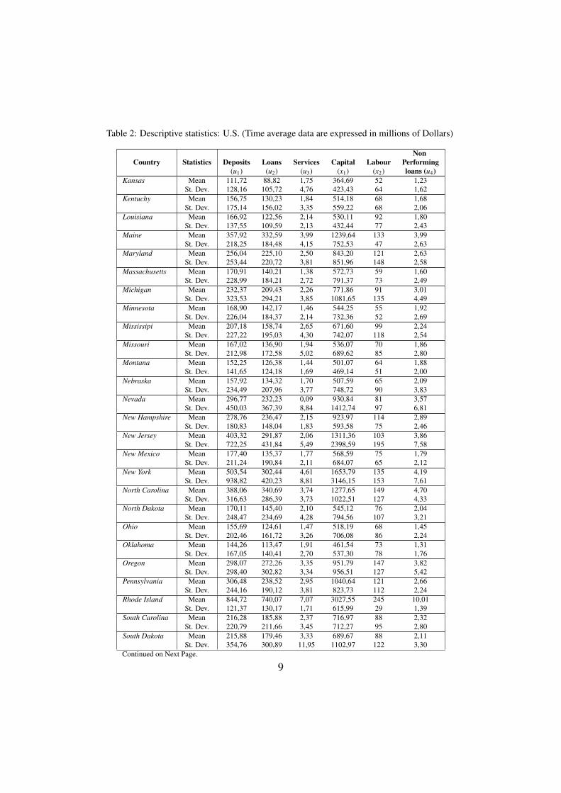
Table 2: Descriptive statistics: U.S. (Time average data are expressed in millions of Dollars)
NonCountry Statistics Deposits Loans Services Capital Labour Performing
(u1) (u2) (u3) (x1) (x2) loans (u4)Kansas Mean 111,72 88,82 1,75 364,69 52 1,23
St. Dev. 128,16 105,72 4,76 423,43 64 1,62Kentuchy Mean 156,75 130,23 1,84 514,18 68 1,68
St. Dev. 175,14 156,02 3,35 559,22 68 2,06Louisiana Mean 166,92 122,56 2,14 530,11 92 1,80
St. Dev. 137,55 109,59 2,13 432,44 77 2,43Maine Mean 357,92 332,59 3,99 1239,64 133 3,99
St. Dev. 218,25 184,48 4,15 752,53 47 2,63Maryland Mean 256,04 225,10 2,50 843,20 121 2,63
St. Dev. 253,44 220,72 3,81 851,96 148 2,58Massachusetts Mean 170,91 140,21 1,38 572,73 59 1,60
St. Dev. 228,99 184,21 2,72 791,37 73 2,49Michigan Mean 232,37 209,43 2,26 771,86 91 3,01
St. Dev. 323,53 294,21 3,85 1081,65 135 4,49Minnesota Mean 168,90 142,17 1,46 544,25 55 1,92
St. Dev. 226,04 184,37 2,14 732,36 52 2,69Mississipi Mean 207,18 158,74 2,65 671,60 99 2,24
St. Dev. 227,22 195,03 4,30 742,07 118 2,54Missouri Mean 167,02 136,90 1,94 536,07 70 1,86
St. Dev. 212,98 172,58 5,02 689,62 85 2,80Montana Mean 152,25 126,38 1,44 501,07 64 1,88
St. Dev. 141,65 124,18 1,69 469,14 51 2,00Nebraska Mean 157,92 134,32 1,70 507,59 65 2,09
St. Dev. 234,49 207,96 3,77 748,72 90 3,83Nevada Mean 296,77 232,23 0,09 930,84 81 3,57
St. Dev. 450,03 367,39 8,84 1412,74 97 6,81New Hampshire Mean 278,76 236,47 2,15 923,97 114 2,89
St. Dev. 180,83 148,04 1,83 593,58 75 2,46New Jersey Mean 403,32 291,87 2,06 1311,36 103 3,86
St. Dev. 722,25 431,84 5,49 2398,59 195 7,58New Mexico Mean 177,40 135,37 1,77 568,59 75 1,79
St. Dev. 211,24 190,84 2,11 684,07 65 2,12New York Mean 503,54 302,44 4,61 1653,79 135 4,19
St. Dev. 938,82 420,23 8,81 3146,15 153 7,61North Carolina Mean 388,06 340,69 3,74 1277,65 149 4,70
St. Dev. 316,63 286,39 3,73 1022,51 127 4,33North Dakota Mean 170,11 145,40 2,10 545,12 76 2,04
St. Dev. 248,47 234,69 4,28 794,56 107 3,21Ohio Mean 155,69 124,61 1,47 518,19 68 1,45
St. Dev. 202,46 161,72 3,26 706,08 86 2,24Oklahoma Mean 144,26 113,47 1,91 461,54 73 1,31
St. Dev. 167,05 140,41 2,70 537,30 78 1,76Oregon Mean 298,07 272,26 3,35 951,79 147 3,82
St. Dev. 298,40 302,82 3,34 956,51 127 5,42Pennsylvania Mean 306,48 238,52 2,95 1040,64 121 2,66
St. Dev. 244,16 190,12 3,81 823,73 112 2,24Rhode Island Mean 844,72 740,07 7,07 3027,55 245 10,01
St. Dev. 121,37 130,17 1,71 615,99 29 1,39South Carolina Mean 216,28 185,88 2,37 716,97 88 2,32
St. Dev. 220,79 211,66 3,45 712,27 95 2,80South Dakota Mean 215,88 179,46 3,33 689,67 88 2,11
St. Dev. 354,76 300,89 11,95 1102,97 122 3,30Continued on Next Page.
9
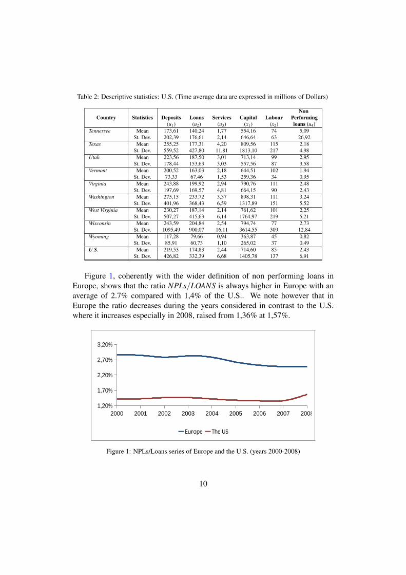
Table 2: Descriptive statistics: U.S. (Time average data are expressed in millions of Dollars)
NonCountry Statistics Deposits Loans Services Capital Labour Performing
(u1) (u2) (u3) (x1) (x2) loans (u4)Tennessee Mean 173,61 140,24 1,77 554,16 74 5,09
St. Dev. 202,39 176,61 2,14 646,64 63 26,92Texas Mean 255,25 177,31 4,20 809,56 115 2,18
St. Dev. 559,52 427,80 11,81 1813,10 217 4,98Utah Mean 223,56 187,50 3,01 713,14 99 2,95
St. Dev. 178,44 153,63 3,03 557,56 87 3,58Vermont Mean 200,52 163,03 2,18 644,51 102 1,94
St. Dev. 73,33 67,46 1,53 259,36 34 0,95Virginia Mean 243,88 199,92 2,94 790,76 111 2,48
St. Dev. 197,69 169,57 4,81 664,15 90 2,43Washington Mean 275,15 233,72 3,37 898,31 111 3,24
St. Dev. 401,96 368,43 6,59 1317,89 151 5,52West Virginia Mean 230,27 187,14 2,14 761,62 101 2,25
St. Dev. 507,27 415,63 6,14 1764,97 219 5,21Wisconsin Mean 243,59 204,84 2,54 794,74 77 2,73
St. Dev. 1095,49 900,07 16,11 3614,55 309 12,84Wyoming Mean 117,28 79,66 0,94 363,87 45 0,82
St. Dev. 85,91 60,73 1,10 265,02 37 0,49U.S. Mean 219,53 174,83 2,44 714,60 85 2,43
St. Dev. 426,82 332,39 6,68 1405,78 137 6,91
Figure 1, coherently with the wider definition of non performing loans inEurope, shows that the ratio NPLs/LOANS is always higher in Europe with anaverage of 2.7% compared with 1,4% of the U.S.. We note however that inEurope the ratio decreases during the years considered in contrast to the U.S.where it increases especially in 2008, raised from 1,36% at 1,57%.
2000 2001 2002 2003 2004 2005 2006 2007 20081,20%
1,70%
2,20%
2,70%
3,20%
NPL/LOANS
Europe The US
Figure 1: NPLs/Loans series of Europe and the U.S. (years 2000-2008)
10
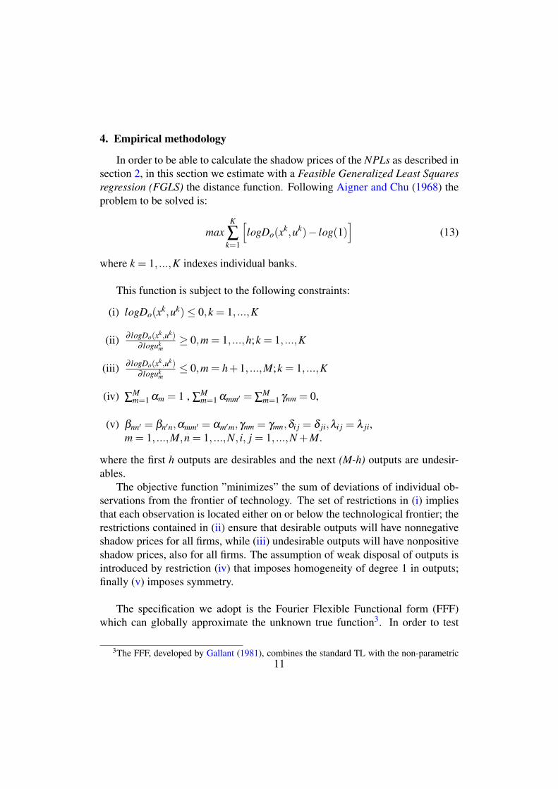
4. Empirical methodology
In order to be able to calculate the shadow prices of the NPLs as described insection 2, in this section we estimate with a Feasible Generalized Least Squaresregression (FGLS) the distance function. Following Aigner and Chu (1968) theproblem to be solved is:
maxK
∑k=1
[logDo(xk,uk)− log(1)
](13)
where k = 1, ...,K indexes individual banks.
This function is subject to the following constraints:
(i) logDo(xk,uk)≤ 0,k = 1, ...,K
(ii) ∂ logDo(xk,uk)∂ loguk
m≥ 0,m = 1, ...,h;k = 1, ...,K
(iii) ∂ logDo(xk,uk)∂ loguk
m≤ 0,m = h+1, ...,M;k = 1, ...,K
(iv) ∑Mm=1 αm = 1 , ∑
Mm=1 αmm′ = ∑
Mm=1 γnm = 0,
(v) βnn′ = βn′n,αmm′ = αm′m,γnm = γmn,δi j = δ ji,λi j = λ ji,m = 1, ...,M,n = 1, ...,N, i, j = 1, ...,N +M.
where the first h outputs are desirables and the next (M-h) outputs are undesir-ables.
The objective function ”minimizes” the sum of deviations of individual ob-servations from the frontier of technology. The set of restrictions in (i) impliesthat each observation is located either on or below the technological frontier; therestrictions contained in (ii) ensure that desirable outputs will have nonnegativeshadow prices for all firms, while (iii) undesirable outputs will have nonpositiveshadow prices, also for all firms. The assumption of weak disposal of outputs isintroduced by restriction (iv) that imposes homogeneity of degree 1 in outputs;finally (v) imposes symmetry.
The specification we adopt is the Fourier Flexible Functional form (FFF)which can globally approximate the unknown true function3. In order to test
3The FFF, developed by Gallant (1981), combines the standard TL with the non-parametric11
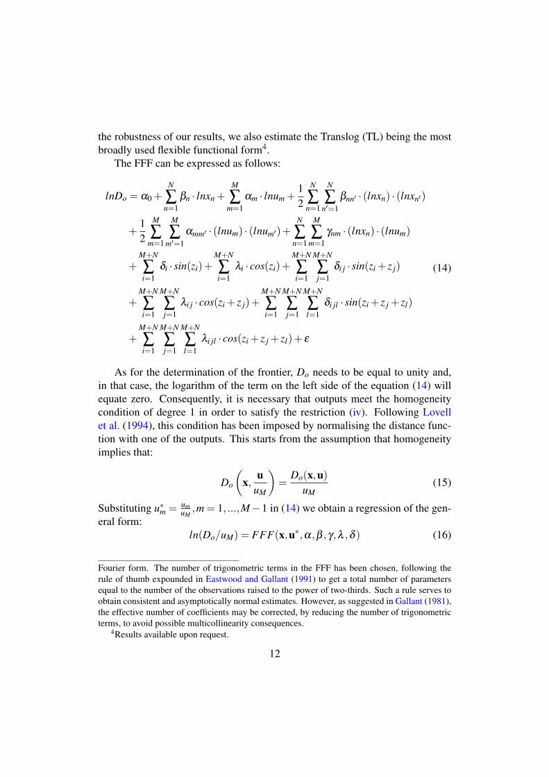
the robustness of our results, we also estimate the Translog (TL) being the mostbroadly used flexible functional form4.
The FFF can be expressed as follows:
lnDo = α0 +N
∑n=1
βn · lnxn +M
∑m=1
αm · lnum +12
N
∑n=1
N
∑n′=1
βnn′ · (lnxn) · (lnxn′)
+12
M
∑m=1
M
∑m′=1
αmm′ · (lnum) · (lnum′)+N
∑n=1
M
∑m=1
γnm · (lnxn) · (lnum)
+M+N
∑i=1
δi · sin(zi)+M+N
∑i=1
λi · cos(zi)+M+N
∑i=1
M+N
∑j=1
δi j · sin(zi + z j)
+M+N
∑i=1
M+N
∑j=1
λi j · cos(zi + z j)+M+N
∑i=1
M+N
∑j=1
M+N
∑l=1
δi jl · sin(zi + z j + zl)
+M+N
∑i=1
M+N
∑j=1
M+N
∑l=1
λi jl · cos(zi + z j + zl)+ ε
(14)
As for the determination of the frontier, Do needs to be equal to unity and,in that case, the logarithm of the term on the left side of the equation (14) willequate zero. Consequently, it is necessary that outputs meet the homogeneitycondition of degree 1 in order to satisfy the restriction (iv). Following Lovellet al. (1994), this condition has been imposed by normalising the distance func-tion with one of the outputs. This starts from the assumption that homogeneityimplies that:
Do
(x,
uuM
)=
Do(x,u)uM
(15)
Substituting u∗m = umuM
,m = 1, ...,M−1 in (14) we obtain a regression of the gen-eral form:
ln(Do/uM) = FFF(x,u∗,α,β ,γ,λ ,δ ) (16)
Fourier form. The number of trigonometric terms in the FFF has been chosen, following therule of thumb expounded in Eastwood and Gallant (1991) to get a total number of parametersequal to the number of the observations raised to the power of two-thirds. Such a rule serves toobtain consistent and asymptotically normal estimates. However, as suggested in Gallant (1981),the effective number of coefficients may be corrected, by reducing the number of trigonometricterms, to avoid possible multicollinearity consequences.
4Results available upon request.
12
where u∗ = ( u1uM
, u2uM
, ..., uM−1uM
).Equation (16) can be written as:
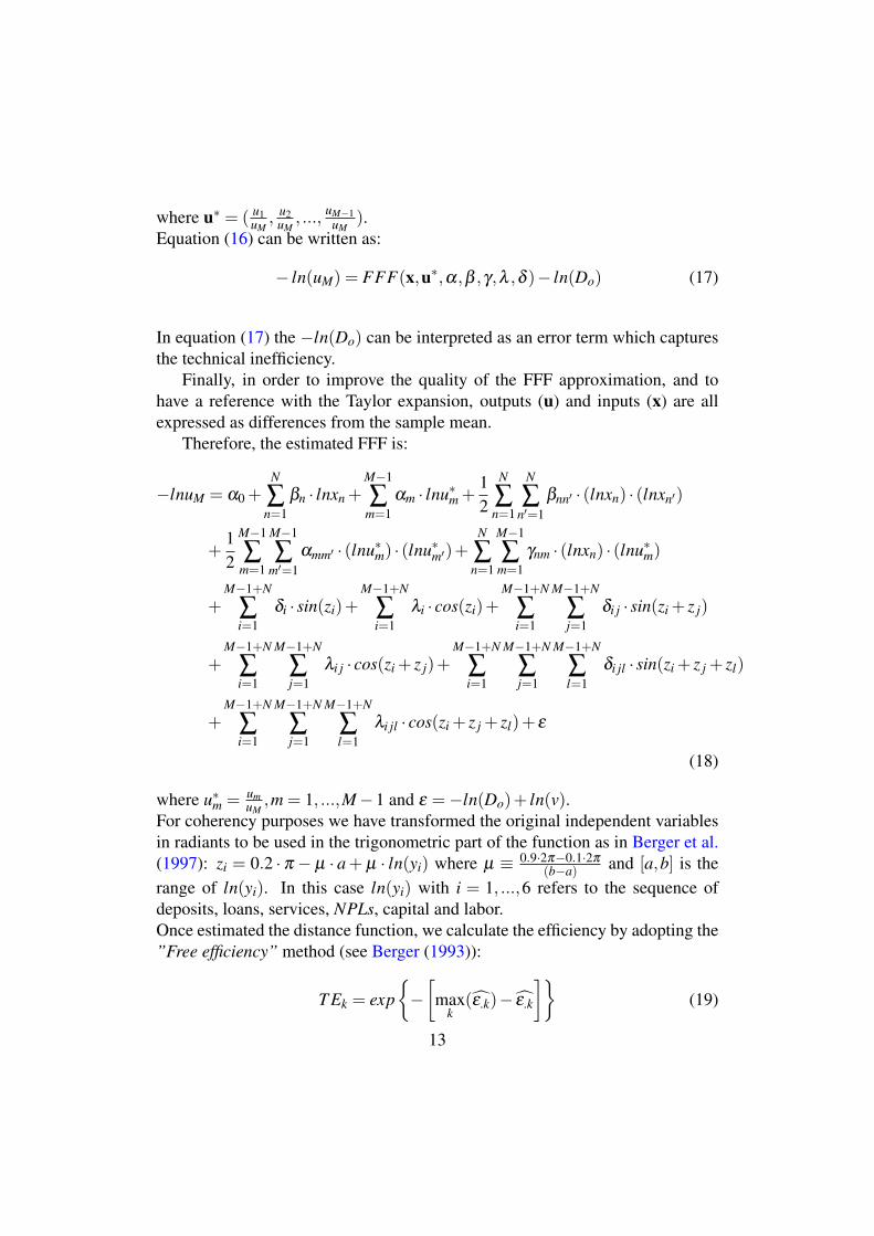
− ln(uM) = FFF(x,u∗,α,β ,γ,λ ,δ )− ln(Do) (17)
In equation (17) the −ln(Do) can be interpreted as an error term which capturesthe technical inefficiency.
Finally, in order to improve the quality of the FFF approximation, and tohave a reference with the Taylor expansion, outputs (u) and inputs (x) are allexpressed as differences from the sample mean.
Therefore, the estimated FFF is:
−lnuM = α0 +N
∑n=1
βn · lnxn +M−1
∑m=1
αm · lnu∗m +12
N
∑n=1
N
∑n′=1
βnn′ · (lnxn) · (lnxn′)
+12
M−1
∑m=1
M−1
∑m′=1
αmm′ · (lnu∗m) · (lnu∗m′)+N
∑n=1
M−1
∑m=1
γnm · (lnxn) · (lnu∗m)
+M−1+N
∑i=1
δi · sin(zi)+M−1+N
∑i=1
λi · cos(zi)+M−1+N
∑i=1
M−1+N
∑j=1
δi j · sin(zi + z j)
+M−1+N
∑i=1
M−1+N
∑j=1
λi j · cos(zi + z j)+M−1+N
∑i=1
M−1+N
∑j=1
M−1+N
∑l=1
δi jl · sin(zi + z j + zl)
+M−1+N
∑i=1
M−1+N
∑j=1
M−1+N
∑l=1
λi jl · cos(zi + z j + zl)+ ε
(18)
where u∗m = umuM
,m = 1, ...,M−1 and ε =−ln(Do)+ ln(v).For coherency purposes we have transformed the original independent variablesin radiants to be used in the trigonometric part of the function as in Berger et al.(1997): zi = 0.2 · π − µ · a+ µ · ln(yi) where µ ≡ 0.9·2π−0.1·2π
(b−a) and [a,b] is therange of ln(yi). In this case ln(yi) with i = 1, ...,6 refers to the sequence ofdeposits, loans, services, NPLs, capital and labor.Once estimated the distance function, we calculate the efficiency by adopting the”Free efficiency” method (see Berger (1993)):
T Ek = exp{−[
maxk
(ε.k)− ε.k
]}(19)
13
where ε.k = ∑t εtk/T.Then the shadow price of NPLs may be found according to the procedure
expounded above.Hence, we estimate the price of loans by assuming that its shadow price is equalto its market price. So, we compute normalized shadow prices r∗(x,u) of de-sirable and undesirable outputs for each bank, using (8), and we calculate theshadow revenue R using the (10). Given the shadow revenue, we derive absoluteshadow prices for NPLs using the (11).
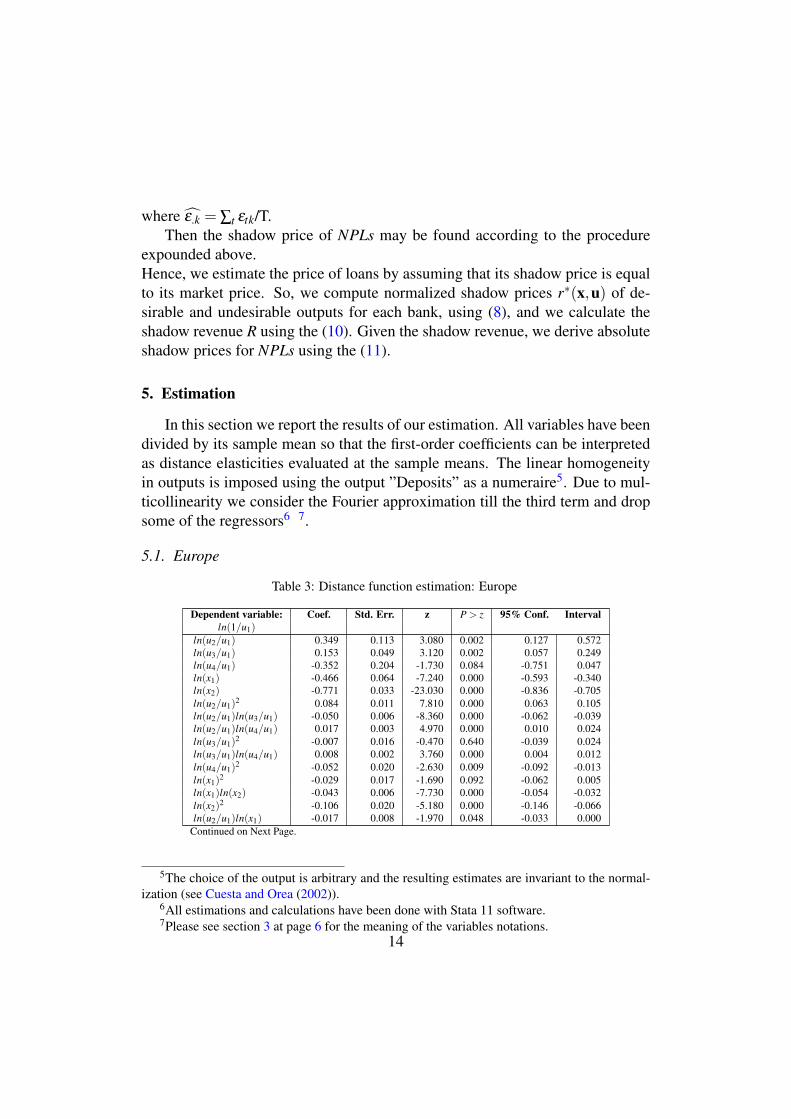
5. Estimation
In this section we report the results of our estimation. All variables have beendivided by its sample mean so that the first-order coefficients can be interpretedas distance elasticities evaluated at the sample means. The linear homogeneityin outputs is imposed using the output ”Deposits” as a numeraire5. Due to mul-ticollinearity we consider the Fourier approximation till the third term and dropsome of the regressors6 7.
5.1. Europe
Table 3: Distance function estimation: Europe
Dependent variable: Coef. Std. Err. z P > z 95% Conf. Intervalln(1/u1)
ln(u2/u1) 0.349 0.113 3.080 0.002 0.127 0.572ln(u3/u1) 0.153 0.049 3.120 0.002 0.057 0.249ln(u4/u1) -0.352 0.204 -1.730 0.084 -0.751 0.047ln(x1) -0.466 0.064 -7.240 0.000 -0.593 -0.340ln(x2) -0.771 0.033 -23.030 0.000 -0.836 -0.705ln(u2/u1)
2 0.084 0.011 7.810 0.000 0.063 0.105ln(u2/u1)ln(u3/u1) -0.050 0.006 -8.360 0.000 -0.062 -0.039ln(u2/u1)ln(u4/u1) 0.017 0.003 4.970 0.000 0.010 0.024ln(u3/u1)
2 -0.007 0.016 -0.470 0.640 -0.039 0.024ln(u3/u1)ln(u4/u1) 0.008 0.002 3.760 0.000 0.004 0.012ln(u4/u1)
2 -0.052 0.020 -2.630 0.009 -0.092 -0.013ln(x1)
2 -0.029 0.017 -1.690 0.092 -0.062 0.005ln(x1)ln(x2) -0.043 0.006 -7.730 0.000 -0.054 -0.032ln(x2)
2 -0.106 0.020 -5.180 0.000 -0.146 -0.066ln(u2/u1)ln(x1) -0.017 0.008 -1.970 0.048 -0.033 0.000
Continued on Next Page.
5The choice of the output is arbitrary and the resulting estimates are invariant to the normal-ization (see Cuesta and Orea (2002)).
6All estimations and calculations have been done with Stata 11 software.7Please see section 3 at page 6 for the meaning of the variables notations.
14
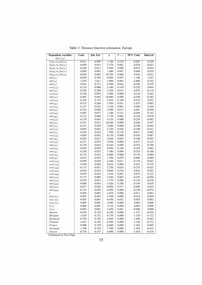
Table 3: Distance function estimation: Europe
Dependent variable: Coef. Std. Err. z P > z 95% Conf. Intervalln(1/u1)
ln(u2/u1)ln(x2) 0.011 0.009 1.180 0.236 -0.007 0.029ln(u3/u1)ln(x1) -0.049 0.015 -3.370 0.001 -0.078 -0.021ln(u3/u1)ln(x2) -0.048 0.012 -3.940 0.000 -0.072 -0.024ln(u4/u1)ln(x1) 0.005 0.003 1.980 0.047 0.000 0.010ln(u4/u1)ln(x2) -0.029 0.003 -10.350 0.000 -0.034 -0.023sin(z2) -0.029 0.549 -0.050 0.957 -1.106 1.047sin(z4) -1.879 1.011 -1.860 0.063 -3.860 0.102sin(z5) -0.054 0.272 -0.200 0.844 -0.586 0.479cos(z22) -0.124 0.086 -1.440 0.149 -0.292 0.044sin(z22) -0.526 0.209 -2.520 0.012 -0.935 -0.116cos(z33) 0.326 0.059 5.490 0.000 0.210 0.443sin(z33) -0.465 0.042 -10.960 0.000 -0.548 -0.382cos(z44) -0.244 0.152 -1.610 0.108 -0.542 0.053sin(z44) -0.515 0.264 -1.950 0.051 -1.033 0.003cos(z55) 0.127 0.039 3.230 0.001 0.050 0.204sin(z55) -0.224 0.090 -2.490 0.013 -0.401 -0.048cos(z66) 0.092 0.077 1.200 0.231 -0.058 0.242sin(z66) -0.212 0.068 -3.130 0.002 -0.344 -0.079cos(z23) -0.176 0.043 -4.110 0.000 -0.259 -0.092sin(z23) 0.251 0.023 10.840 0.000 0.206 0.297sin(z24) -0.121 0.030 -4.040 0.000 -0.180 -0.062cos(z25) -0.095 0.043 -2.220 0.026 -0.180 -0.011sin(z25) 0.036 0.024 1.500 0.135 -0.011 0.082cos(z26) 0.005 0.042 0.130 0.898 -0.076 0.087sin(z26) -0.054 0.027 -2.010 0.045 -0.108 -0.001cos(z35) -0.271 0.074 -3.650 0.000 -0.417 -0.125sin(z35) -0.270 0.042 -6.420 0.000 -0.353 -0.188cos(z36) -0.050 0.059 -0.850 0.396 -0.165 0.065sin(z36) -0.256 0.035 -7.380 0.000 -0.324 -0.188cos(z56) -0.132 0.022 -5.880 0.000 -0.176 -0.088sin(z56) 0.032 0.018 1.760 0.079 -0.004 0.069cos(z222) -0.099 0.039 -2.540 0.011 -0.176 -0.023cos(z333) 0.260 0.030 8.610 0.000 0.201 0.319cos(z444) -0.115 0.051 -2.250 0.024 -0.215 -0.015cos(z555) -0.010 0.016 -0.640 0.524 -0.043 0.022cos(z666) 0.078 0.023 3.410 0.001 0.033 0.123sin(z222) -0.175 0.060 -2.940 0.003 -0.292 -0.058sin(z333) -0.079 0.021 -3.770 0.000 -0.120 -0.038sin(z444) -0.088 0.054 -1.620 0.106 -0.194 0.018sin(z555) -0.017 0.026 -0.650 0.517 -0.069 0.035sin(z666) -0.132 0.030 -4.450 0.000 -0.190 -0.074t -0.005 0.003 -1.670 0.096 -0.011 0.001t(u2/u1) -0.007 0.002 -4.700 0.000 -0.010 -0.004t(u3/u1) -0.001 0.001 -0.450 0.652 -0.003 0.002t(u4/u1) 0.005 0.001 4.940 0.000 0.003 0.006t(x1) 0.006 0.001 4.110 0.000 0.003 0.008t(x2) -0.003 0.001 -1.870 0.061 -0.006 0.000Austria -0.928 0.150 -6.180 0.000 -1.223 -0.634Belgium -1.019 0.151 -6.730 0.000 -1.316 -0.722Denmark -0.756 0.150 -5.050 0.000 -1.050 -0.463Finland -1.031 0.158 -6.540 0.000 -1.340 -0.722France -0.988 0.150 -6.600 0.000 -1.282 -0.695Germany -1.108 0.150 -7.390 0.000 -1.402 -0.814Greece -0.718 0.153 -4.690 0.000 -1.018 -0.418
Continued on Next Page.
15
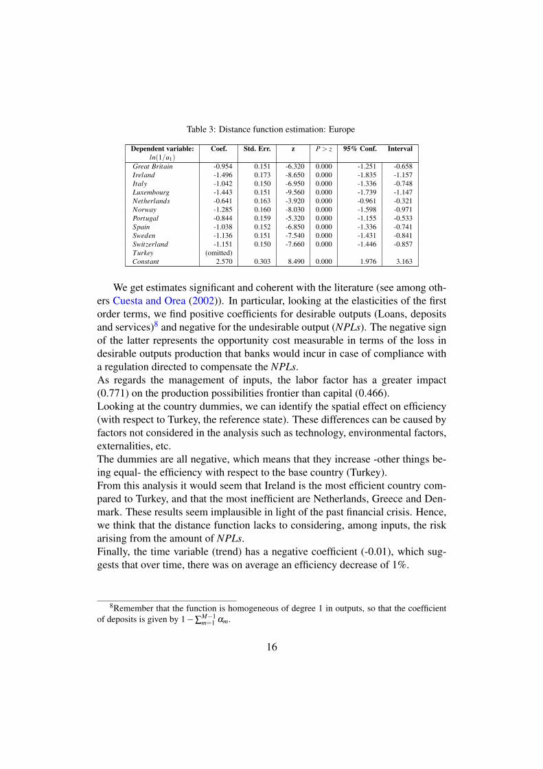
Table 3: Distance function estimation: Europe
Dependent variable: Coef. Std. Err. z P > z 95% Conf. Intervalln(1/u1)
Great Britain -0.954 0.151 -6.320 0.000 -1.251 -0.658Ireland -1.496 0.173 -8.650 0.000 -1.835 -1.157Italy -1.042 0.150 -6.950 0.000 -1.336 -0.748Luxembourg -1.443 0.151 -9.560 0.000 -1.739 -1.147Netherlands -0.641 0.163 -3.920 0.000 -0.961 -0.321Norway -1.285 0.160 -8.030 0.000 -1.598 -0.971Portugal -0.844 0.159 -5.320 0.000 -1.155 -0.533Spain -1.038 0.152 -6.850 0.000 -1.336 -0.741Sweden -1.136 0.151 -7.540 0.000 -1.431 -0.841Switzerland -1.151 0.150 -7.660 0.000 -1.446 -0.857Turkey (omitted)Constant 2.570 0.303 8.490 0.000 1.976 3.163
We get estimates significant and coherent with the literature (see among oth-ers Cuesta and Orea (2002)). In particular, looking at the elasticities of the firstorder terms, we find positive coefficients for desirable outputs (Loans, depositsand services)8 and negative for the undesirable output (NPLs). The negative signof the latter represents the opportunity cost measurable in terms of the loss indesirable outputs production that banks would incur in case of compliance witha regulation directed to compensate the NPLs.As regards the management of inputs, the labor factor has a greater impact(0.771) on the production possibilities frontier than capital (0.466).Looking at the country dummies, we can identify the spatial effect on efficiency(with respect to Turkey, the reference state). These differences can be caused byfactors not considered in the analysis such as technology, environmental factors,externalities, etc.The dummies are all negative, which means that they increase -other things be-ing equal- the efficiency with respect to the base country (Turkey).From this analysis it would seem that Ireland is the most efficient country com-pared to Turkey, and that the most inefficient are Netherlands, Greece and Den-mark. These results seem implausible in light of the past financial crisis. Hence,we think that the distance function lacks to considering, among inputs, the riskarising from the amount of NPLs.Finally, the time variable (trend) has a negative coefficient (-0.01), which sug-gests that over time, there was on average an efficiency decrease of 1%.
8Remember that the function is homogeneous of degree 1 in outputs, so that the coefficientof deposits is given by 1−∑
M−1m=1 αm.
16
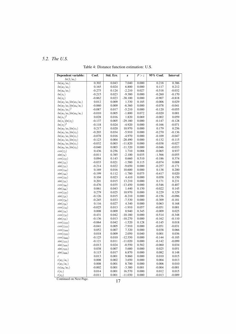
5.2. The U.S.
Table 4: Distance function estimation: U.S.
Dependent variable: Coef. Std. Err. z P > z 95% Conf. Intervalln(1/u1)
ln(u2/u1) 0.302 0.043 7.040 0.000 0.218 0.386ln(u3/u1) 0.165 0.024 6.800 0.000 0.117 0.212ln(u4/u1) -0.275 0.124 -2.210 0.027 -0.518 -0.032ln(x1) -0.215 0.023 -9.380 0.000 -0.260 -0.170ln(x2) -0.862 0.023 -38.100 0.000 -0.907 -0.818ln(u2/u1)ln(u3/u1) 0.012 0.009 1.330 0.185 -0.006 0.029ln(u2/u1)ln(u4/u1) -0.060 0.009 -6.360 0.000 -0.078 -0.041ln(u3/u1)
2 -0.087 0.017 -5.210 0.000 -0.120 -0.055ln(u3/u1)ln(u4/u1) -0.010 0.005 -1.800 0.072 -0.020 0.001ln(x1)
2 0.028 0.016 1.820 0.069 -0.002 0.059ln(x1)ln(x2) -0.137 0.005 -29.180 0.000 -0.147 -0.128ln(x2)
2 -0.118 0.024 -4.920 0.000 -0.166 -0.071ln(u2/u1)ln(x1) 0.217 0.020 10.970 0.000 0.179 0.256ln(u2/u1)ln(x2) -0.203 0.034 -5.910 0.000 -0.270 -0.136ln(u3/u1)ln(x1) -0.078 0.016 -4.970 0.000 -0.109 -0.047ln(u3/u1)ln(x2) -0.123 0.004 -28.490 0.000 -0.132 -0.115ln(u4/u1)ln(x1) -0.032 0.003 -11.820 0.000 -0.038 -0.027ln(u4/u1)ln(x2) -0.040 0.003 -11.320 0.000 -0.046 -0.033cos(z2) 0.436 0.256 1.710 0.088 -0.065 0.937sin(z4) -0.811 0.385 -2.100 0.035 -1.566 -0.055cos(z22) 0.094 0.143 0.660 0.510 -0.186 0.374sin(z22) -0.033 0.021 -1.580 0.115 -0.074 0.008sin(z33) -0.214 0.022 -9.650 0.000 -0.257 -0.171cos(z44) 0.169 0.016 10.600 0.000 0.138 0.200sin(z44) -0.199 0.112 -1.780 0.075 -0.417 0.020cos(z55) 0.104 0.023 4.410 0.000 0.058 0.150sin(z55) 0.201 0.015 13.210 0.000 0.171 0.231cos(z66) -0.476 0.035 -13.450 0.000 -0.546 -0.407sin(z66) 0.061 0.043 1.440 0.150 -0.022 0.145cos(z25) 0.279 0.025 10.970 0.000 0.229 0.329sin(z25) -0.126 0.015 -8.210 0.000 -0.156 -0.096cos(z26) -0.245 0.033 -7.530 0.000 -0.309 -0.181sin(z26) 0.116 0.027 4.340 0.000 0.063 0.168cos(z34) -0.025 0.013 -1.910 0.057 -0.051 0.001sin(z34) 0.008 0.009 0.940 0.345 -0.009 0.025cos(z35) -0.431 0.042 -10.180 0.000 -0.514 -0.348sin(z35) -0.136 0.013 -10.270 0.000 -0.162 -0.110cos(z222) -0.064 0.042 -1.520 0.128 -0.145 0.018cos(z333) -0.041 0.005 -7.910 0.000 -0.051 -0.031cos(z444) 0.052 0.007 7.320 0.000 0.038 0.066cos(z555) 0.018 0.009 2.050 0.040 0.001 0.036cos(z666) -0.125 0.010 -12.550 0.000 -0.144 -0.105sin(z333) -0.121 0.011 -11.020 0.000 -0.142 -0.099sin(z444) -0.013 0.024 -0.550 0.582 -0.060 0.034sin(z555) 0.038 0.007 5.680 0.000 0.025 0.051sin(z666) 0.115 0.017 6.870 0.000 0.082 0.148t 0.013 0.001 9.860 0.000 0.010 0.015t(u2/u1) 0.008 0.002 3.650 0.000 0.004 0.013t(u3/u1) 0.008 0.001 8.700 0.000 0.006 0.010ty(u4/u1) -0.002 0.001 -3.380 0.001 -0.004 -0.001t(x1) 0.014 0.001 16.570 0.000 0.012 0.015t(x2) -0.011 0.001 -11.030 0.000 -0.013 -0.009
Continued on Next Page. 17
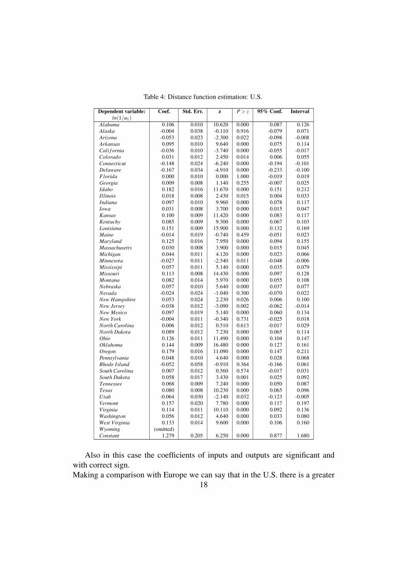
Table 4: Distance function estimation: U.S.
Dependent variable: Coef. Std. Err. z P > z 95% Conf. Intervalln(1/u1)
Alabama 0.106 0.010 10.620 0.000 0.087 0.126Alaska -0.004 0.038 -0.110 0.916 -0.079 0.071Arizona -0.053 0.023 -2.300 0.022 -0.098 -0.008Arkansas 0.095 0.010 9.640 0.000 0.075 0.114Cali f ornia -0.036 0.010 -3.740 0.000 -0.055 -0.017Colorado 0.031 0.012 2.450 0.014 0.006 0.055Connecticut -0.148 0.024 -6.240 0.000 -0.194 -0.101Delaware -0.167 0.034 -4.910 0.000 -0.233 -0.100Florida 0.000 0.010 0.000 1.000 -0.019 0.019Georgia 0.009 0.008 1.140 0.255 -0.007 0.025Idaho 0.182 0.016 11.670 0.000 0.151 0.212Illinois 0.018 0.008 2.430 0.015 0.004 0.033Indiana 0.097 0.010 9.960 0.000 0.078 0.117Iowa 0.031 0.008 3.700 0.000 0.015 0.047Kansas 0.100 0.009 11.420 0.000 0.083 0.117Kentuchy 0.085 0.009 9.300 0.000 0.067 0.103Louisiana 0.151 0.009 15.900 0.000 0.132 0.169Maine -0.014 0.019 -0.740 0.459 -0.051 0.023Maryland 0.125 0.016 7.950 0.000 0.094 0.155Massachusetts 0.030 0.008 3.900 0.000 0.015 0.045Michigan 0.044 0.011 4.120 0.000 0.023 0.066Minnesota -0.027 0.011 -2.540 0.011 -0.048 -0.006Mississipi 0.057 0.011 5.140 0.000 0.035 0.079Missouri 0.113 0.008 14.430 0.000 0.097 0.128Montana 0.082 0.014 5.970 0.000 0.055 0.108Nebraska 0.057 0.010 5.640 0.000 0.037 0.077Nevada -0.024 0.024 -1.040 0.300 -0.070 0.022New Hampshire 0.053 0.024 2.230 0.026 0.006 0.100New Jersey -0.038 0.012 -3.090 0.002 -0.062 -0.014New Mexico 0.097 0.019 5.140 0.000 0.060 0.134New York -0.004 0.011 -0.340 0.731 -0.025 0.018North Carolina 0.006 0.012 0.510 0.613 -0.017 0.029North Dakota 0.089 0.012 7.230 0.000 0.065 0.114Ohio 0.126 0.011 11.490 0.000 0.104 0.147Oklahoma 0.144 0.009 16.480 0.000 0.127 0.161Oregon 0.179 0.016 11.090 0.000 0.147 0.211Pennsylvania 0.048 0.010 4.640 0.000 0.028 0.068Rhode Island -0.052 0.058 -0.910 0.364 -0.166 0.061South Carolina 0.007 0.012 0.560 0.574 -0.017 0.031South Dakota 0.058 0.017 3.430 0.001 0.025 0.092Tennessee 0.068 0.009 7.240 0.000 0.050 0.087Texas 0.080 0.008 10.230 0.000 0.065 0.096Utah -0.064 0.030 -2.140 0.032 -0.123 -0.005Vermont 0.157 0.020 7.780 0.000 0.117 0.197Virginia 0.114 0.011 10.110 0.000 0.092 0.136Washington 0.056 0.012 4.640 0.000 0.033 0.080West Virginia 0.133 0.014 9.600 0.000 0.106 0.160Wyoming (omitted)Constant 1.279 0.205 6.250 0.000 0.877 1.680
Also in this case the coefficients of inputs and outputs are significant andwith correct sign.Making a comparison with Europe we can say that in the U.S. there is a greater
18
impact of labor (-0.86 vs -0.77) and the opposite for capital (-0.22 vs -0.47).This means that the labor factor (capital factor) in the U.S. performs more (less)than in Europe, in fact, increasing the latter the negative effect on efficiency ismore limited. This is probably due to the lower dimension of capital employedin Europe compared to labor.If we analyze the spatial dummies, there are two groups of countries placingabove and below the baseline country (Wyoming) in terms of efficiency level.This leads us to question on the inefficiencies and responsibilities of countriesand banks.
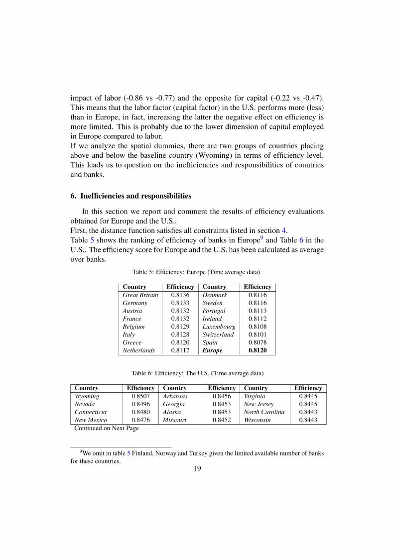
6. Inefficiencies and responsibilities
In this section we report and comment the results of efficiency evaluationsobtained for Europe and the U.S..First, the distance function satisfies all constraints listed in section 4.Table 5 shows the ranking of efficiency of banks in Europe9 and Table 6 in theU.S.. The efficiency score for Europe and the U.S. has been calculated as averageover banks.
Table 5: Efficiency: Europe (Time average data)
Country Efficiency Country EfficiencyGreat Britain 0.8136 Denmark 0.8116Germany 0.8133 Sweden 0.8116Austria 0.8132 Portugal 0.8113France 0.8132 Ireland 0.8112Belgium 0.8129 Luxembourg 0.8108Italy 0.8128 Switzerland 0.8101Greece 0.8120 Spain 0.8078Netherlands 0.8117 Europe 0.8120
Table 6: Efficiency: The U.S. (Time average data)
Country Efficiency Country Efficiency Country EfficiencyWyoming 0.8507 Arkansas 0.8456 Virginia 0.8445Nevada 0.8496 Georgia 0.8453 New Jersey 0.8445Connecticut 0.8480 Alaska 0.8453 North Carolina 0.8443New Mexico 0.8476 Missouri 0.8452 Wisconsin 0.8443Continued on Next Page
9We omit in table 5 Finland, Norway and Turkey given the limited available number of banksfor these countries.
19
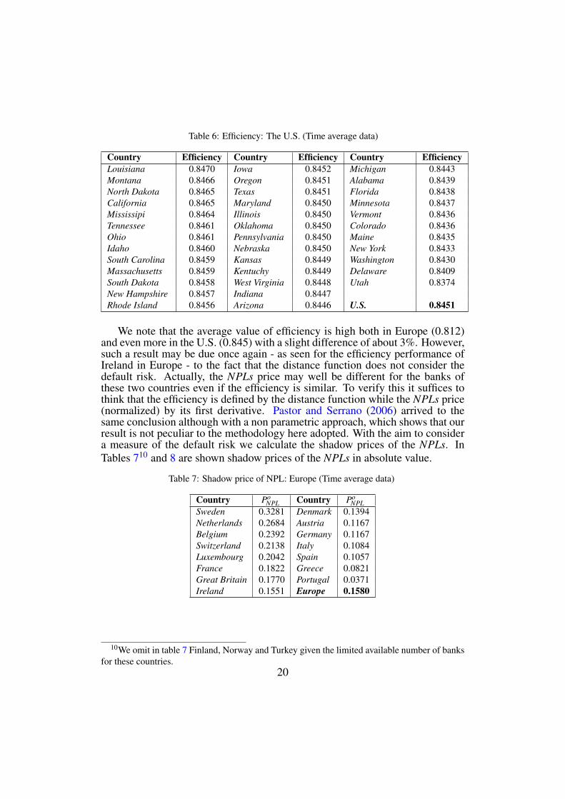
Table 6: Efficiency: The U.S. (Time average data)
Country Efficiency Country Efficiency Country EfficiencyLouisiana 0.8470 Iowa 0.8452 Michigan 0.8443Montana 0.8466 Oregon 0.8451 Alabama 0.8439North Dakota 0.8465 Texas 0.8451 Florida 0.8438California 0.8465 Maryland 0.8450 Minnesota 0.8437Mississipi 0.8464 Illinois 0.8450 Vermont 0.8436Tennessee 0.8461 Oklahoma 0.8450 Colorado 0.8436Ohio 0.8461 Pennsylvania 0.8450 Maine 0.8435Idaho 0.8460 Nebraska 0.8450 New York 0.8433South Carolina 0.8459 Kansas 0.8449 Washington 0.8430Massachusetts 0.8459 Kentuchy 0.8449 Delaware 0.8409South Dakota 0.8458 West Virginia 0.8448 Utah 0.8374New Hampshire 0.8457 Indiana 0.8447Rhode Island 0.8456 Arizona 0.8446 U.S. 0.8451
We note that the average value of efficiency is high both in Europe (0.812)and even more in the U.S. (0.845) with a slight difference of about 3%. However,such a result may be due once again - as seen for the efficiency performance ofIreland in Europe - to the fact that the distance function does not consider thedefault risk. Actually, the NPLs price may well be different for the banks ofthese two countries even if the efficiency is similar. To verify this it suffices tothink that the efficiency is defined by the distance function while the NPLs price(normalized) by its first derivative. Pastor and Serrano (2006) arrived to thesame conclusion although with a non parametric approach, which shows that ourresult is not peculiar to the methodology here adopted. With the aim to considera measure of the default risk we calculate the shadow prices of the NPLs. InTables 710 and 8 are shown shadow prices of the NPLs in absolute value.
Table 7: Shadow price of NPL: Europe (Time average data)
Country PoNPL Country Po
NPLSweden 0.3281 Denmark 0.1394Netherlands 0.2684 Austria 0.1167Belgium 0.2392 Germany 0.1167Switzerland 0.2138 Italy 0.1084Luxembourg 0.2042 Spain 0.1057France 0.1822 Greece 0.0821Great Britain 0.1770 Portugal 0.0371Ireland 0.1551 Europe 0.1580
10We omit in table 7 Finland, Norway and Turkey given the limited available number of banksfor these countries.
20
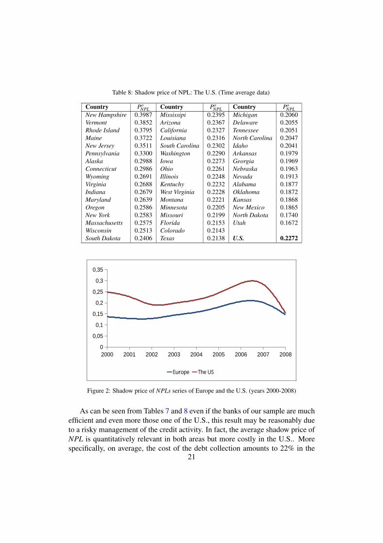
Table 8: Shadow price of NPL: The U.S. (Time average data)
Country PoNPL Country Po
NPL Country PoNPL
New Hampshire 0.3987 Mississipi 0.2395 Michigan 0.2060Vermont 0.3852 Arizona 0.2367 Delaware 0.2055Rhode Island 0.3795 California 0.2327 Tennessee 0.2051Maine 0.3722 Louisiana 0.2316 North Carolina 0.2047New Jersey 0.3511 South Carolina 0.2302 Idaho 0.2041Pennsylvania 0.3300 Washington 0.2290 Arkansas 0.1979Alaska 0.2988 Iowa 0.2273 Georgia 0.1969Connecticut 0.2986 Ohio 0.2261 Nebraska 0.1963Wyoming 0.2691 Illinois 0.2248 Nevada 0.1913Virginia 0.2688 Kentuchy 0.2232 Alabama 0.1877Indiana 0.2679 West Virginia 0.2228 Oklahoma 0.1872Maryland 0.2639 Montana 0.2221 Kansas 0.1868Oregon 0.2586 Minnesota 0.2205 New Mexico 0.1865New York 0.2583 Missouri 0.2199 North Dakota 0.1740Massachusetts 0.2575 Florida 0.2153 Utah 0.1672Wisconsin 0.2513 Colorado 0.2143South Dakota 0.2406 Texas 0.2138 U.S. 0.2272
2000 2001 2002 2003 2004 2005 2006 2007 20080
0,05
0,1
0,15
0,2
0,25
0,3
0,35
Shadow price of NPL
Europe The US
Figure 2: Shadow price of NPLs series of Europe and the U.S. (years 2000-2008)
As can be seen from Tables 7 and 8 even if the banks of our sample are muchefficient and even more those one of the U.S., this result may be reasonably dueto a risky management of the credit activity. In fact, the average shadow price ofNPL is quantitatively relevant in both areas but more costly in the U.S.. Morespecifically, on average, the cost of the debt collection amounts to 22% in the
21
U.S. and 16% in Europe.The graph in Figure 2 shows how in both cases the price of NPLs has greatlyrisen since 2002 with a peak between years 2006 and 2007 and has fallen during2008 for the regulatory actions of the governments as a consequence of the crisis.In 2008 the two NPLs prices become almost equal.
But who is the responsible between countries and banks?
To answer this question we move from the consideration that if the bankrisk is controlled across countries by each single bank, then the banking systemwould be reliable. On the other hand, if the risk doesnt vary across banks pereach single country, then the regulation imposed by countries is effective. If theautonomy of the banks to manage with the risk across countries is high, thenthe responsibility is more referable to banks. This problem can be analyzed interms of between-variances, applied to the variable representing the risk, evalu-ated across countries (σ2
Bcountries) and across banks (σ2
Bbanks): the former represents
the capacity of the banks to control the risk and the latter the capacity of coun-ties to set appropriate regulations capable to control the risk. We normalize theformer to the latter to make a comparison. We consider two variables of interest,NPLs/L and NPLs price, and conclude that the higher is the σ2
Bcountries/σ2
Bbanksratio
the less the attention devoted by countries to the control the risk of the bankingsystem.
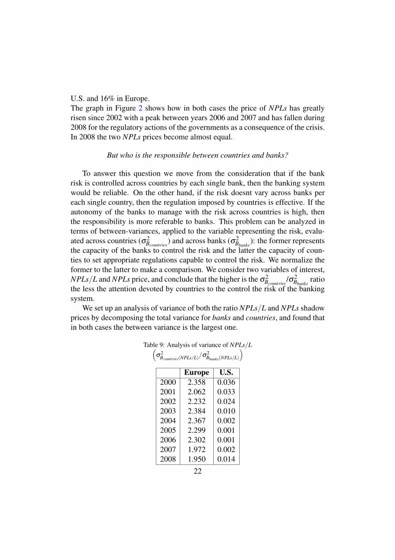
We set up an analysis of variance of both the ratio NPLs/L and NPLs shadowprices by decomposing the total variance for banks and countries, and found thatin both cases the between variance is the largest one.
Table 9: Analysis of variance of NPLs/L(σ2
Bcountries(NPLs/L)/σ2Bbanks(NPLs/L)
)Europe U.S.
2000 2.358 0.0362001 2.062 0.0332002 2.232 0.0242003 2.384 0.0102004 2.367 0.0022005 2.299 0.0012006 2.302 0.0012007 1.972 0.0022008 1.950 0.014
22
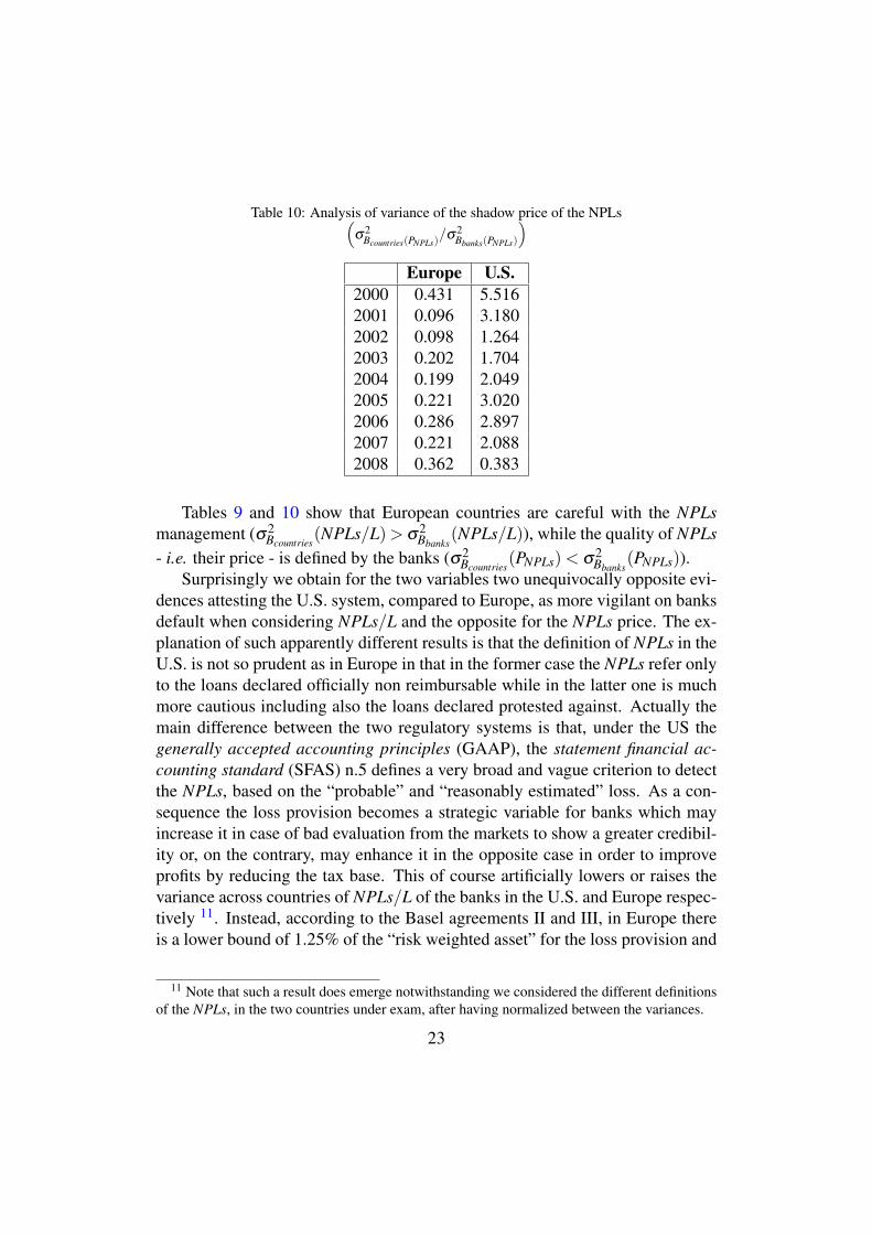
Table 10: Analysis of variance of the shadow price of the NPLs(σ2
Bcountries(PNPLs)/σ2
Bbanks(PNPLs)
)Europe U.S.
2000 0.431 5.5162001 0.096 3.1802002 0.098 1.2642003 0.202 1.7042004 0.199 2.0492005 0.221 3.0202006 0.286 2.8972007 0.221 2.0882008 0.362 0.383
Tables 9 and 10 show that European countries are careful with the NPLsmanagement (σ2
Bcountries(NPLs/L)> σ2
Bbanks(NPLs/L)), while the quality of NPLs
- i.e. their price - is defined by the banks (σ2Bcountries
(PNPLs)< σ2Bbanks
(PNPLs)).Surprisingly we obtain for the two variables two unequivocally opposite evi-
dences attesting the U.S. system, compared to Europe, as more vigilant on banksdefault when considering NPLs/L and the opposite for the NPLs price. The ex-planation of such apparently different results is that the definition of NPLs in theU.S. is not so prudent as in Europe in that in the former case the NPLs refer onlyto the loans declared officially non reimbursable while in the latter one is muchmore cautious including also the loans declared protested against. Actually themain difference between the two regulatory systems is that, under the US thegenerally accepted accounting principles (GAAP), the statement financial ac-counting standard (SFAS) n.5 defines a very broad and vague criterion to detectthe NPLs, based on the “probable” and “reasonably estimated” loss. As a con-sequence the loss provision becomes a strategic variable for banks which mayincrease it in case of bad evaluation from the markets to show a greater credibil-ity or, on the contrary, may enhance it in the opposite case in order to improveprofits by reducing the tax base. This of course artificially lowers or raises thevariance across countries of NPLs/L of the banks in the U.S. and Europe respec-tively 11. Instead, according to the Basel agreements II and III, in Europe thereis a lower bound of 1.25% of the “risk weighted asset” for the loss provision and
11 Note that such a result does emerge notwithstanding we considered the different definitionsof the NPLs, in the two countries under exam, after having normalized between the variances.
23
an upper bound of 50% of the “regulatory capital requirements”12.
7. Final Remarks and Policy implications
In the analysis developed we discuss about credit market, country’s policyactions and efficiency of the banking system.
With regard to the credit market our analysis identifies an increasing NPLsprice in the considered period as showed in Figure 2 and underlines that in theusual risk analysis is difficult to take properly into account this trend, being theNPLs price not normally observable.
Moreover, comparing the NPLs price with the interest rate of loans, wereckon that banks measure incorrectly the real risk and the cost to recover theNPLs by fixing an interest rate that does not contain adequately the effectiveNPLs price. Given such an excessive cost, it would be appropriate to monitorthe lending banks policy with apposite regulations which take into account theNPLs price as a margin to be stored in case of loss.
A second point is that there is the necessity to homogenize the definitionof NPLs in order to avoid that the ratio NPLs/L is systemically and artificiallydifferent between countries, like in the case considered here where where suchratio is sensibly lower in the US compared to Europe. On the contrary, ouranalysis shows that the NPLs price is always higher in the U.S. with respect toEurope.
A significant result of our research the importance of countries in explainingthe recent financial crisis. From Table 10 in the U.S. theσ2
Bcountries(PNPLs)/σ2
Bbanks(PNPLs) ratio is very high from 2000 to 2007 showing a
great responsibility of the countries in not having preserved a homogeneous riskmanagement of banks (low σ2
Bbanks(PNPLs)). This is confirmed by the low NPLs/L
ratio obtained in 2008 when the U.S. government intervened by introducingmarket-wide support measures and assisting failing financial institutions. In lightof these facts, legislative measures for monitoring the banks would be importantto avoid future crisis. In Europe, instead, this supervision was already effectiveas showed by the low σ2
Bcountries(PNPLs)/σ2
Bbanks(PNPLs) ratio. Therefore, in order to
improve the quality of loans in Europe the direction is to look for some improve-ments in terms of efficiency. In effect, in such a respect we note that in Europe therisk strategies, concerning the ratio between non performing loans and loans, arevery different among banks (high σ2
Bcountries(NPLs/L)/σ2
Bbanks(NPLs/L)), which
12Moreover, still in the definition of the “risk weighted asset” the weights are more compellingin Europe than in the US.
24
is likely to be referred to different levels of efficiency in the loans management.Actually, Tables 5 and 6 show a lower efficiency in Europe than in the U.S..A possible explanation of this fact is that European banks try to bypass thestricter rules on the NPLs registration by improving profits with a reduction inthe regulatory capital13. Hence, an intriguing question, possibly of future re-search, should be to understand how much part of the banks efficiency is dueto the correct proportion between the undervalued NPLs/L and the regulatorycapital, or how much of inefficiency is due to the correct evaluation of NPLs/Lin contrast to a low regulatory capital. A way to solve this problem would be topenalize risky banks by asking them to pay as a penalty the NPLs price. Thiswould be a counterincentive to the expansion of NPLs as a strategy to gathermore funds irrespective of the risk.
8. Conclusion
The analysis conducted in this paper showed that the recent bank crisis couldbe anticipated if appropriate indicators would have been used. We propose herethe NPLs price which is not observable. Our econometric methodology basedon the Fourier expansion validates significantly the theoretical set up adopted.Actually we found that the market interest rates do not adequately account forthe risk of loans loss. Further, Europe and the U.S. have different peculiaritiesconcerning the inefficiencies of the bank system and the responsibilities of thetwo countries. We found more countries’ responsibility in terms of low regu-lations for the U.S. and a slightly more inefficiency for Europe. A proposal tomonitor both aspects is to penalize risky banks by asking to pay as a penalty theNPLs price.
Acknoledgments
The authors wish to thank Daniela Palatta and Ronald Gallant for helpfulcomments and suggestions. Financial support is from University of Rome LaSapienza and MIUR.
13Slovik (2012) finds the same result on the base of an analysis of the ratio between the risk-weighted assets to total asset.
25
BibliographyAigner, D. J., Chu, S. F., 1968. On estimating the industry production function. American Eco-
nomic Review 58, 826–839.Berger, A. N., 1993. ’distribution free’ estimates of efficiency of the u.s. banking industry and
tests of the standard distributional assumptions. Finance and Economics Discussion Series188, Board of Governors of the Federal Reserve System (U.S.).
Berger, A. N., DeYoung, R., 1997. Problem loans and cost efficiency in commercial banks. Tech.rep.
Berger, A. N., Leusner, J. H., Mingo, J. J., 1997. The efficiency of bank branches. Journal ofMonetary Economics 40 (1), 141 – 162.
Cuesta, R. A., Orea, L., 2002. Mergers and technical efficiency in spanish savings banks: Astochastic distance function approach. Journal of Banking & Finance 26 (12), 2231–2247.
Eastwood, B. J., Gallant, A. R., 1991. Adaptive rules for seminonparametric estimators thatachieve asymptotic normality. Econometric Theory 7 (03), 307–340.
Fare, R., 1988. Fundamentals of production theory. Lecture notes in economics and mathematicalsystems. Springer.
Fare, R., Knox Lovell, C. A., October 1978. Measuring the technical efficiency of production.Journal of Economic Theory 19 (1), 150–162.
Fare, R., Primont, D., 1995. Multi-output production and duality: theory and applications.Kluwer Academic Publishers.
Farrell, M. J., 1957. The measurement of productive efficiency. Journal Of The Royal StatisticalSociety Series A General 120 (3), 253–290.
Gallant, A. R., February 1981. On the bias in flexible functional forms and an essentially unbi-ased form : The fourier flexible form. Journal of Econometrics 15 (2), 211–245.
Hughes, J. P., Mester, L. J., 1993. A quality and risk-adjusted cost function for banks: Evidenceon the too-big-to-fail doctrine. Journal of Productivity Analysis 4, 293–315.
Jacobsen, S. E., June 1972. On shephard’s duality theorem. Journal of Economic Theory 4 (3),458–464.
Lovell, K., Richardson, S., Travers, P., Wood, L., 1994. Resources and functions: A new view ofinequality in australia. School of Economics Working Papers 1990-07, University of Adelaide,School of Economics.
Maggi, B., Guida, M., 2011. Modelling non-performing loans probability in the commercialbanking system: efficiency and effectiveness related to credit risk in italy. Empirical Eco-nomics 41, 269–291.
Pastor, J., 2002. Credit risk and efficiency in the european banking system: A three-stage analy-sis. Applied Financial Economics 12 (12), 895–911.
Pastor, J., Serrano, L., 2005. Efficiency, endogenous and exogenous credit risk in the bankingsystems of the euro area. Applied Financial Economics 15 (9), 631–649.
Pastor, J., Serrano, L., 2006. The effect of specialisation on banks’ efficiency: An internationalcomparison. International Review of Applied Economics 20 (1), 125–149.
Shephard, R., 1970. Theory of cost and production functions. Princeton studies in mathematicaleconomics. Princeton University Press.
Slovik, P., 2012. Systematically important banks and capital regulations challenges. DepartmentWorking Papers, OECD Publishing 916.
26