HAL Id: hal-01889235https://hal.archives-ouvertes.fr/hal-01889235v2

Submitted on 18 Oct 2020

HAL is a multi-disciplinary open accessarchive for the deposit and dissemination of sci-entific research documents, whether they are pub-lished or not. The documents may come fromteaching and research institutions in France orabroad, or from public or private research centers.

L’archive ouverte pluridisciplinaire HAL, estdestinée au dépôt et à la diffusion de documentsscientifiques de niveau recherche, publiés ou non,émanant des établissements d’enseignement et derecherche français ou étrangers, des laboratoirespublics ou privés.

Asymptotic approximations for the close evaluation ofdouble-layer potentials

Camille Carvalho, Shilpa Khatri, Arnold Kim

To cite this version:Camille Carvalho, Shilpa Khatri, Arnold Kim. Asymptotic approximations for the close evaluation ofdouble-layer potentials. SIAM Journal on Scientific Computing, Society for Industrial and AppliedMathematics, 2020, 42, pp.A504-A533. �hal-01889235v2�

Asymptotic approximations for the close evaluation of

double-layer potentials

Camille Carvalho∗ Shilpa Khatri ∗ Arnold D. Kim ∗

Abstract

When using boundary integral equation methods to solve a boundary value problem, the eval-uation of the solution near the boundary is challenging to compute because the layer potentialsthat represent the solution are nearly-singular integrals. To address this close evaluation problem,we develop a new numerical method by applying an asymptotic analysis of these nearly singularintegrals and obtaining an asymptotic approximation. We derive the asymptotic approximationfor the case of the double-layer potential in two and three dimensions, representing the solutionof the interior Dirichlet problem for Laplace’s equation. By doing so, we obtain an asymptoticapproximation given by the Dirichlet data at the boundary point nearest to the interior evaluationpoint plus a nonlocal correction. We present the numerical methods using this asymptotic approx-imation, and we demonstrate the efficiency and accuracy of these methods and the asymptoticapproximation through several examples. These examples show that the numerical method basedon the asymptotic approximation accurately approximates the close evaluation of the double-layerpotential while requiring only modest computational resources.

1 Introduction

The close evaluation problem refers to the nonuniform error produced by high-order quadrature rulesused in boundary integral equation methods. High-order quadrature rules attain spectral accuracywhen computing the solution, represented by layer potentials, far from the boundary, but incur avery large error when computing the solution close to the boundary. This large error incurred whenevaluating layer potentials close to the boundary is called the close evaluation problem. It is wellunderstood that this growth in error is due to the fact that the integrand of the layer potentialsbecomes increasingly peaked as the point of evaluation approaches the boundary. In fact, when thedistance between the evaluation point and its closest boundary point is smaller than the distancebetween quadrature points on the boundary for a fixed-order quadrature rule, the quadrature pointsdo not adequately resolve the peak of the integrand and therefore produce an O(1) error.

Accurate evaluations of layer potentials close to the boundary of the domain are needed for a widerange of applications, including the modeling of swimming micro-organisms, droplet suspensions, andblood cells in Stokes flow [8, 18, 23, 30], and to predict accurate measurements of the electromagneticnear-field in the field of plasmonics [22] for nano-antennas [3, 26] and sensors [24,28].

Several computational methods have been developed to address this close evaluation problem.Schwab and Wendland [29] have developed a boundary extraction method based on a Taylor seriesexpansion of the layer potentials. Beale and Lai [10] have developed a method that first regularizesthe nearly singular kernel of the layer potential and then adds corrections for both the discretizationand the regularization. Beale et al. [11] have extended the regularization method to three-dimensionalproblems. Helsing and Ojala [16] developed a method that combines a globally compensated quadraturerule and interpolation to achieve very accurate results over all regions of the domain. Barnett [9] has

∗Applied Mathematics Unit, School of Natural Sciences, University of California, Merced, 5200 North Lake Road,Merced, CA 95343

1

used surrogate local expansions with centers placed near, but not on, the boundary. Klockner et al. [20]introduced Quadrature By Expansion (QBX), which uses expansions about accurate evaluation pointsfar away from the boundary to compute accurate evaluations close to it. There have been severalsubsequent studies of QBX [1,2, 14,27,31] that have extended its use and characterized its behavior.

Recently, the authors have applied asymptotic analysis to study the close evaluation problem. Fortwo-dimensional problems, the authors developed a method that used matched asymptotic expansionsfor the kernel of the layer potential [12]. In that method, the asymptotic expansion that captures thepeaked behavior of the kernel (namely, the peaked behavior of the integrand of the layer potential)can be integrated exactly and the relatively smooth remainder is integrated numerically, resultingin a highly accurate method. For three-dimensional problems, the authors have developed a simple,three-step method for computing layer potentials [13]. This method involves first rotating the spher-ical coordinate system used to compute the layer potential so that the boundary point at which theintegrand becomes singular is aligned with the north pole. By studying the asymptotic behavior ofthe integral, they found that integration with respect to the azimuthal angle after the initial rotationis a natural averaging operation that regularizes the integral, and allows for a high-order quadraturerule to be used for the integral with respect to the polar angle. This numerical method was shownto achieve an error that decays quadratically with the distance to the boundary provided that theunderlying boundary integral equation for the density is sufficiently resolved. In this work, we carryout an asymptotic analysis of the close evaluation of the double-layer potential for the interior Dirich-let problem for Laplace’s equation in two and three dimensions. By doing so, we derive asymptoticapproximations that provide valuable insight into the inherent challenges of the close evaluation prob-lem. These asymptotic approximations are given by the Dirichlet data at the boundary point closestto the evaluation point plus a nonlocal correction. It is the nonlocal correction that makes the closeevaluation problem challenging to address. The asymptotic analysis leads to an explicit expressionfor this nonlocal correction and suggests a natural way to accurately and efficiently compute it. Wedevelop new, explicit numerical methods for computing the close evaluation using these asymptoticapproximations. We provide several examples that demonstrate that these methods are consistentwith the expected accuracy from the asymptotic analysis. The remainder of this paper is as follows.We precisely define the close evaluation problem for the double-layer potential and state the expectedleading-order asymptotic behavior of the double-layer potential in Section 2. We give the derivationin two dimensions in Section 3 and three dimensions in Section 4. We describe the new numericalmethods using the asymptotic approximations for the close evaluation of the double-layer potential inSection 5. We give several examples demonstrating the accuracy of this numerical method in Section 6.Section 7 gives our conclusions. The Appendices provide details of the computations used throughoutthis paper: Appendix A establishes additional results we have used to justify the obtained asymptoticapproximations of Sections 3-4, Appendix B gives details of how we rotate spherical integrals, andAppendix C gives a useful derivation of the spherical Laplacian.

2 Motivation and results of asymptotic analysis

Consider a simply connected, open set, denoted by D ⊂ Rn with n = 2, 3, with an analytic closeboundary, B, and let D = D ∪ B. Given some smooth data f ∈ C2(B), we write the functionu ∈ C2(D) ∩ C1(D) satisfying the interior Dirichlet problem,

∆u = 0 in D, (2.1a)

u = f on B, (2.1b)

as the double-layer potential,

u(x) =1

2n−1π

∫B

νy · (x− y)

|x− y|nµ(y)dσy, x ∈ D, n = 2, 3. (2.2)

2

Β

D

y*

ν*

Δs

x2

x1

O(Δs)

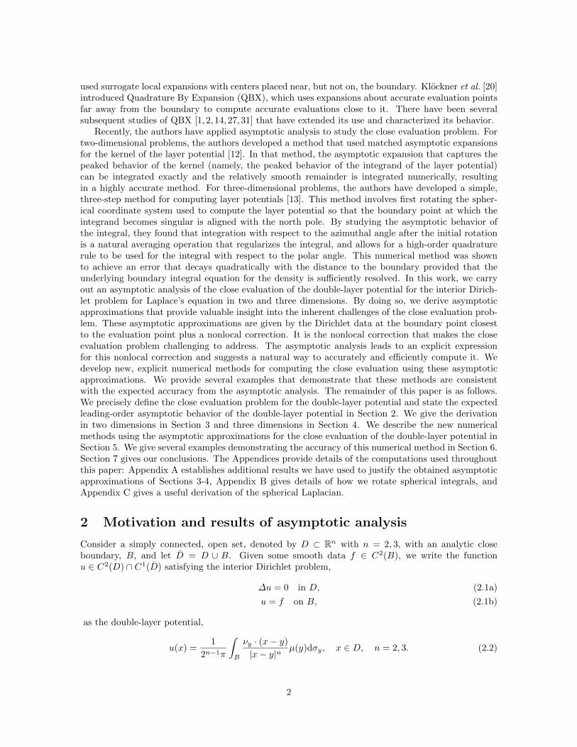
Figure 1: 2D sketch showing the finite length scale, ∆s, of the discretization for (2.1) which leads tothe close evaluation problem. For the point x1 which is farther than ∆s from the boundary, we findthat the kernel is well resolved with the boundary grid. However, for the same boundary grid, we findthat the kernel is poorly resolved for x2, which is closer to the boundary than ∆s. In each plot on

the right, the kernel K(xi − y(s)) :=νy·(xi−y(s))|xi−y(s)|2 , i = 1, 2, is plotted in blue, and a piece-wise linear

approximation using a fixed ∆s grid is plotted in dashed orange.

Here, νy denotes the unit outward normal at y ∈ B, dσy denotes the boundary element, and µ ∈ C2(B)denotes the density. The double-layer potential given by (2.2) satisfies (2.1a). To require that (2.2)satisfies (2.1b), we first recognize that it satisfies the following jump condition [15,21],

limx→y?∈Bx∈D

1

2n−1π

∫B

νy · (x− y)

|x− y|nµ(y)dσy =

1

2n−1π

∫B

νy · (y? − y)

|y? − y|nµ(y)dσy −

1

2µ(y?). (2.3)

In light of the jump condition (2.3) and the boundary condition (2.1b), µ satisfies the boundary integralequation,

1

2n−1π

∫B

νy · (y? − y)

|y? − y|nµ(y)dσy −

1

2µ(y?) = f(y?), y? ∈ B. (2.4)

2.1 The close evaluation problem

The close evaluation problem refers to the large-error resulting from computing the solution close tothe boundary using a high-order quadrature rule at a fixed order. The close evaluation problem for(2.1) can be understood intuitively. Laplace’s equation has no intrinsic finite length scale. This lack offinite length scale is manifest in the kernel of (2.4), which is singular at y = y?. When one introduces afinite discretization of the boundary, one effectively is introducing a finite length scale into the problem.Let ∆s denote this finite length scale corresponding to the boundary discretization. For evaluationpoints in the domain farther than ∆s from the boundary, the kernel of (2.2) is smooth and a fixed∆s boundary discretization adequately resolves it. In contrast, for evaluation points in the domaincloser than ∆s from the boundary, the kernel is nearly singular and cannot be adequately resolved bythis fixed boundary grid. Figure 1 shows these differences. This description of the close evaluationproblem provides valuable insight. First, we understand that the size of the region exhibiting the

3

close evaluation problem scales with the boundary discretization. Hence, in the limit as the numberof boundary points grows, this region shrinks proportionally, which is simply a consequence of theconvergence of the numerical method. However, we also understand that the close evaluation problemexists for any fixed boundary discretization and is therefore unavoidable for any practical calculation.

As stated in the introduction, there have been several methods developed that successfully addressthe close evaluation problem. However, because the close evaluation problem is an intrinsic propertyof the boundary integral equation formulation and because close evaluations near the boundary areimportant for many physical applications, we are motivated to consider an alternative method to studythe close evaluation problem. The method presented here closely follows the intuitive explanation abovein which the discretization introduces a finite length scale into the problem. In particular, we applyasymptotic analysis to study the evaluation of the double-layer potential in the limit as the evaluationpoint x approaches a point on the boundary y? and use this analysis to develop an accurate numericalmethod for these close evaluation points.

2.2 Preliminaries

To prepare to state our results of the asymptotic analysis, we introduce some notation. We referthe reader to the Definition 1.1 (“Big-oh”), Definition 1.2 (“Big-oh” near z0), Definition 1.4 (“Little-oh”), Definition 1.9 (Asymptotic sequence), and Definition 1.10 (Asymptotic expansion) from Miller’stext [25], and to [17, Section 2.5] for more details. Given some functions f and g defined over someset D, we will use the notation f � g to indicate that f(x) = o(g(x)) whenever x ∈ D, and x tendsto some x0 ∈ D [25, Definition 1.4]. Given a function f , we construct an asymptotic expansion of theform

f(x) ∼∞∑n=0

εnfn(x), ε→ 0+.

In other words, we only consider the asymptotic sequence {εn}∞n=0 as ε→ 0+ [25, Definition 1.10]. Wewill make use of the notation f(x) = f0(x) + εf1(x) +O(ε2), to denote the “asymptotic approximationof f(x) to order ε2 in the limit as ε→ 0+.” With these definitions and notations established, we statethe the formal asymptotic analysis in the next subsection.

2.3 Results of asymptotic analysis

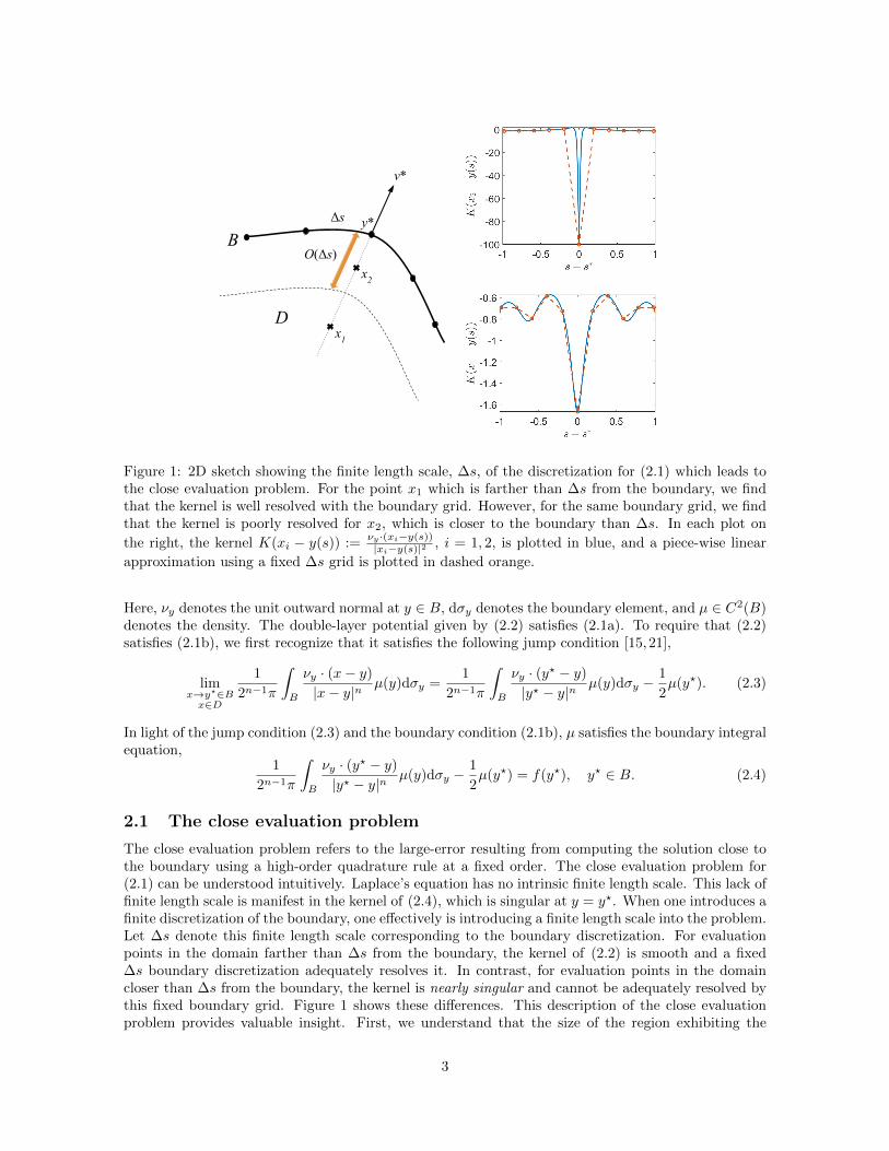
To study the close evaluation of (2.2), we introduce the parameter, ε, in the evaluation point xaccording to

x = y? − ε`ν?, (2.5)

and consider the asymptotic limit of ε → 0+. Here, y? ∈ B denotes the closest point to x on theboundary, ν? denotes the unit, outward normal at y?, and ` denotes a characteristic length of theproblem, like the radius of curvature at y? (see Fig. 2). Since the solution of (2.1) continuouslyapproaches its boundary data from within D,

u(x) = u(y? − ε`ν?) = f(y?) + εU(y?; ε). (2.6)

To determine an expression for U , we substitute (2.2) evaluated at (2.5) for u(y?− ε`ν?) and (2.4) forf(y?) into (2.6), and find that

U(y?; ε) = ε−1[

1

2µ(y?) +

1

2n−1π

∫B

[νy · (yd − ε`ν?)|yd − ε`ν?|n

− νy · yd|yd|n

]µ(y)dσy

], (2.7)

where we have introduced the notation, yd = y? − y. Next, we make use of Gauss’ theorem [15],

1

2n−1π

∫B

νy · (x− y)

|x− y|ndσy =

−1 x ∈ D,− 1

2 x ∈ B,0 x 6∈ D,

(2.8)

4

y?

x

ν?

B

D

εl

y?

x

ν?

B

D

εl

Figure 2: Sketch of the quantities introduced in (2.5) to study evaluation points close to the boundaryin 2D (left) and in 3D (right).

to write1

2µ(y?) = µ(y?)− 1

2µ(y?)

= − 1

2n−1π

∫B

νy · (yd − ε`ν?)|yd − ε`ν?|n

µ(y?)dσy +1

2n−1π

∫B

νy · yd|yd|n

µ(y?)dσy.(2.9)

Substituting (2.9) into (2.7) yields

U(y?; ε) =1

2n−1π

∫B

ε−1[νy · (yd − ε`ν?)|yd − ε`ν?|n

− νy · yd|yd|n

][µ(y)− µ(y?)]dσy. (2.10)

Let

K(yd, ε) =1

2n−1π

νy · (yd − εlν?)|yd − εlν?|n

. (2.11)

Then (2.10) can be rewritten as

U(y?; ε) =

∫B

K(yd, ε)−K(yd, 0)

ε[µ(y)− µ(y?)]dσy, (2.12)

which reveals that the kernel of U(y?; ε) is proportional to ∂εK(yd, 0). This observation motivates us toseek asymptotic expansions for U(y?; ε). Note that U(y?; ε) is a weakly singular integral that providesan important contribution to the double-layer potential off and on the boundary. The asymptoticanalysis results of this paper are stated in the two conjectures below.

Conjecture 2.1. (2D Asymptotic Approximation) Consider a bounded open set D ⊂ R2 with ananalytic closed boundary B that can be parameterized as y = y(t) for 0 ≤ t ≤ 2π. Let y? = y(0). Forf ∈ C2(B), the solution of (2.1) at x = y? − ε`ν? is given by u(y? − ε`ν?) = f(y?) + εU(y?; ε), andthe asymptotic approximation of U(y?; ε) to O(ε2) is

U(y?; ε) = L1[µ](y?) + εL2[µ](y?)

− ε`2y′(0) · y′′(0)

4|y′(0)|4dµ(y(t))

dt

∣∣∣∣t=0

+ ε`2

4|y′(0)|2d2µ(y(t))

dt2

∣∣∣∣t=0

+O(ε2), (2.13)

with

L1[µ](y?) = `

∫B

2(νy · yd)(ν? · yd)− νy · ν?|yd|2

|yd|4[µ(y)− µ(y?)] dσy, (2.14)

5

and

L2[µ](y?) = `2∫B

(νy · yd)[4(ν? · yd)2

]− 2|yd|2(νy · ν?)(ν? · yd)|yd|6

[µ(y)− µ(y?)] dσy. (2.15)

By replacing U in u(y? − ε`ν?) = f(y?) + εU(y?; ε) with (2.13), we obtain the asymptotic approx-imation of u(y? − ε`ν?) to O(ε3).

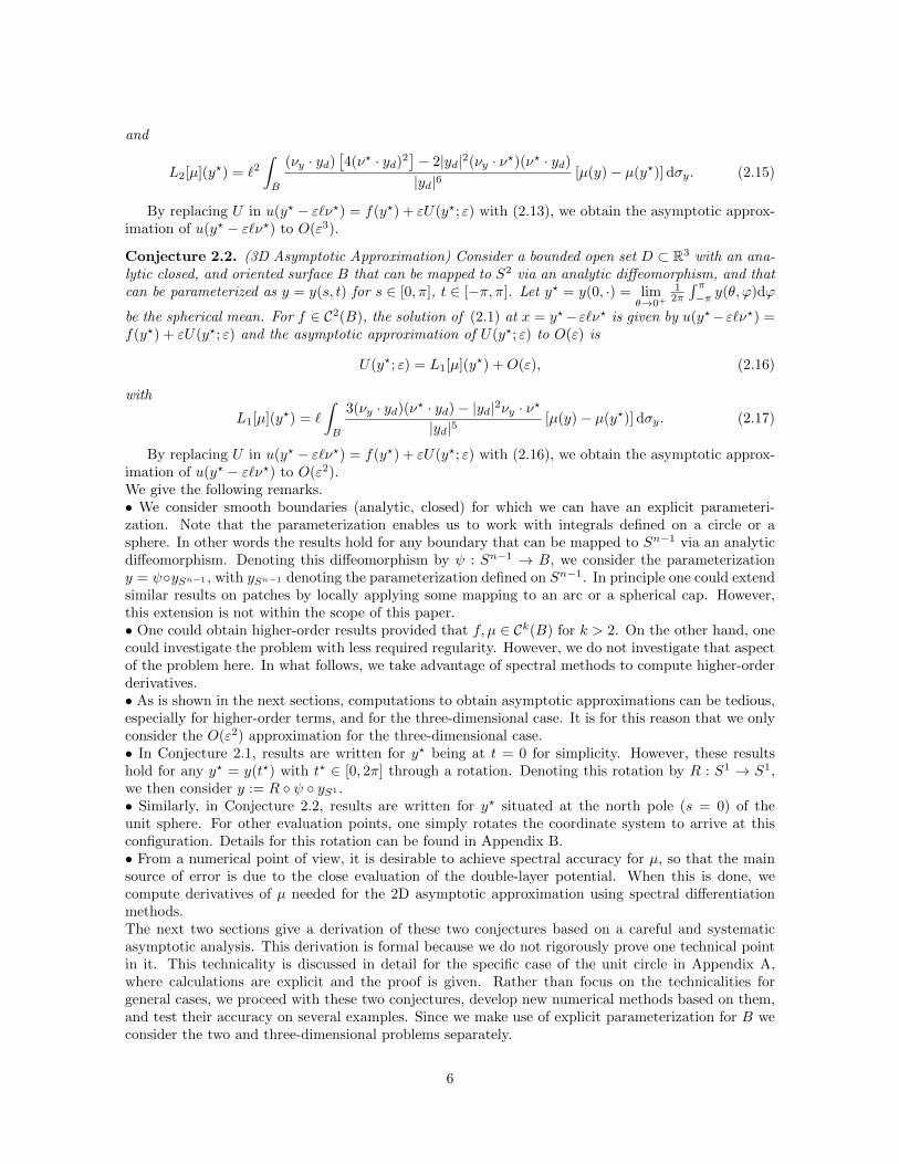
Conjecture 2.2. (3D Asymptotic Approximation) Consider a bounded open set D ⊂ R3 with an ana-lytic closed, and oriented surface B that can be mapped to S2 via an analytic diffeomorphism, and thatcan be parameterized as y = y(s, t) for s ∈ [0, π], t ∈ [−π, π]. Let y? = y(0, ·) = lim

θ→0+

12π

∫ π−π y(θ, ϕ)dϕ

be the spherical mean. For f ∈ C2(B), the solution of (2.1) at x = y?−ε`ν? is given by u(y?−ε`ν?) =f(y?) + εU(y?; ε) and the asymptotic approximation of U(y?; ε) to O(ε) is

U(y?; ε) = L1[µ](y?) +O(ε), (2.16)

with

L1[µ](y?) = `

∫B

3(νy · yd)(ν? · yd)− |yd|2νy · ν?

|yd|5[µ(y)− µ(y?)] dσy. (2.17)

By replacing U in u(y? − ε`ν?) = f(y?) + εU(y?; ε) with (2.16), we obtain the asymptotic approx-imation of u(y? − ε`ν?) to O(ε2).We give the following remarks.• We consider smooth boundaries (analytic, closed) for which we can have an explicit parameteri-zation. Note that the parameterization enables us to work with integrals defined on a circle or asphere. In other words the results hold for any boundary that can be mapped to Sn−1 via an analyticdiffeomorphism. Denoting this diffeomorphism by ψ : Sn−1 → B, we consider the parameterizationy = ψ◦ySn−1 , with ySn−1 denoting the parameterization defined on Sn−1. In principle one could extendsimilar results on patches by locally applying some mapping to an arc or a spherical cap. However,this extension is not within the scope of this paper.• One could obtain higher-order results provided that f, µ ∈ Ck(B) for k > 2. On the other hand, onecould investigate the problem with less required regularity. However, we do not investigate that aspectof the problem here. In what follows, we take advantage of spectral methods to compute higher-orderderivatives.• As is shown in the next sections, computations to obtain asymptotic approximations can be tedious,especially for higher-order terms, and for the three-dimensional case. It is for this reason that we onlyconsider the O(ε2) approximation for the three-dimensional case.• In Conjecture 2.1, results are written for y? being at t = 0 for simplicity. However, these resultshold for any y? = y(t?) with t? ∈ [0, 2π] through a rotation. Denoting this rotation by R : S1 → S1,we then consider y := R ◦ ψ ◦ yS1 .• Similarly, in Conjecture 2.2, results are written for y? situated at the north pole (s = 0) of theunit sphere. For other evaluation points, one simply rotates the coordinate system to arrive at thisconfiguration. Details for this rotation can be found in Appendix B.• From a numerical point of view, it is desirable to achieve spectral accuracy for µ, so that the mainsource of error is due to the close evaluation of the double-layer potential. When this is done, wecompute derivatives of µ needed for the 2D asymptotic approximation using spectral differentiationmethods.The next two sections give a derivation of these two conjectures based on a careful and systematicasymptotic analysis. This derivation is formal because we do not rigorously prove one technical pointin it. This technicality is discussed in detail for the specific case of the unit circle in Appendix A,where calculations are explicit and the proof is given. Rather than focus on the technicalities forgeneral cases, we proceed with these two conjectures, develop new numerical methods based on them,and test their accuracy on several examples. Since we make use of explicit parameterization for B weconsider the two and three-dimensional problems separately.

6

3 Asymptotic approximations in two dimensions

We give a derivation of the O(ε) term in Conjecture 2.1, i.e. L1[µ](y?) defined in (2.14), and thencomment on how to compute the O(ε2) terms in Conjecture 2.1. As stated in Conjecture 2.1, weassume B to be an analytic, closed curve on the plane. We introduce the parameter t ∈ [−π, π] suchthat y = y(t) and y? = y(0). In terms of this parameterization, (2.10) is given by

U(y?; ε) =1

2π

∫ π

−πε−1K(t; ε)[µ(t)− µ(0)]dt, (3.1)

with µ(t) = µ(y(t)), µ(0) = µ(y(0)) = µ(y?), and

K(t; ε) =

[ν(t) · (yd(t)− ε`ν?)|yd(t)− ε`ν?|2

− ν(t) · yd(t)|yd(t)|2

]J(t), (3.2)

with ν(t) = ν(y(t)), yd(t) = y(0)− y(t), and J(t) = |y′(t)|. Note that ν? = ν(0).To determine the asymptotic expansion for U , we write

U(y?; ε) = U in(y?; ε) + Uout(y?; ε), (3.3)

with the inner expansion, U in, and the outer expansion, Uout, given by

U in(y?; ε) =1

2π

∫ √ε/2−√ε/2

ε−1K(t; ε) [µ(t)− µ(0)] dt, (3.4a)

Uout(y?; ε) =1

2π

∫ −√ε/2−π

ε−1K(t; ε) [µ(t)− µ(0)] dt

+1

2π

∫ π

√ε/2

ε−1K(t; ε) [µ(t)− µ(0)] dt.

(3.4b)

The inner expansion involves integration over an O(ε1/2) portion of the boundary about y?, whereasthe outer expansion involves integration over the remaining portion of the boundary. The followingresults also hold if one considers O(εα) portion of the boundary with 0 < α < 1. Since the innerand outer expansions come from splitting the integral over the boundary, we refer to this procedureas an integral splitting method for computing the asymptotic expansion for the close evaluation of thedouble-layer potential.

We determine the leading-order asymptotic behaviors of U in and Uout in the subsections below.Then, we combine those results to obtain the asymptotic approximation for the double-layer potentialin two dimensions, and discuss higher-order asymptotic approximations. The procedure we use herefollows that by Hinch [17, Section 3]. We have developed Mathematica notebooks that contain thepresented calculations, available in a GitHub repository [19]. In what follows we assume that K and µhave asymptotic expansions in the limit as ε→ 0+ (as described in Section 2.2) and that the remainderof the asymptotic approximation to O(εn) with n > 1 yields an O(εn−1) after integration. Details ofthe proof are given for the unit circle in Appendix A.

3.1 Inner expansion

To determine the leading-order asymptotic behavior of U in, we substitute t = εT into (3.4a), andobtain

U in(y?; ε) =1

2π

∫ 1/(2√ε)

−1/(2√ε)

K(εT ; ε) [µ(εT )− µ(0)] dT. (3.5)

Recognizing that ν(εT ) = ν? +O(ε) and yd(εT ) = −εTy′(0) +O(ε2) with ν? · y′(0) = 0, we find thatby expanding K(εT ; ε) about ε = 0 that

K(εT ; ε) = − ε−1`J(0)

T 2J2(0) + `2+O(1). (3.6)

7

Using the fact that this leading-order behavior is even in T , and expanding µ about ε = 0, we substitutethese expansions into (3.5) to get

U in(y?; ε) =1

2π

∫ 1/(2√ε)

−1/(2√ε)

[− ε−1`J(0)

T 2J2(0) + `2+O(1)

][µ(εT )− µ(0)] dT

=1

2π

∫ 1/(2√ε)

0

[− ε−1`J(0)

T 2J2(0) + `2+O(1)

][µ(εT ) + µ(−εT )− 2µ(0)] dT

=1

2π

∫ 1/(2√ε)

0

[− ε−1`J(0)

T 2J2(0) + `2+O(1)

] [ε2T 2µ′′(0) +O(ε4)

]dT

=1

2π

∫ 1/(2√ε)

0

[− εT 2`J(0)

T 2J2(0) + `2µ′′(0) +O(ε2)

]dT.

(3.7)

Above, we have obtained an asymptotic approximation of the integrand to O(ε2) (see Section 2.2).Following the procedure given by Hinch [17, Section 3.4], after integrating (see [19] and Appendix A)and expanding about ε = 0, we find the leading-order asymptotic behavior of U in to be

U in(y?; ε) = −√ε`

4πJ(0)µ′′(0) +O(ε). (3.8)

Remark 1. The obtained asymptotic expansion used in 3.7 is nonuniform. One needs to establishuniform convergence to rigorously prove that the remainder of the asymptotic approximation to orderε2, after integration, is O(ε). Obtaining this result in general is not straightforward. We give detailsof the proof for the case of the unit circle in Appendix A.

3.2 Outer expansion

To determine the leading-order asymptotic behavior of Uout, we expand K(t; ε) about ε = 0 and findthat K(t; ε) = [εK1(t) +O(ε2)]J(t), with

K1(t) = `2(ν(t) · yd(t))(ν? · yd(t))− ν(t) · ν?|yd(t)|2

|yd(t)|4. (3.9)

Substituting this expansion into (3.4b), we find that

Uout(y?; ε) =1

2π

∫ −√ε/2−π

K1(t) [µ(t)− µ(0)] J(t)dt

+1

2π

∫ π

√ε/2

K1(t) [µ(t)− µ(0)] J(t)dt+O(ε). (3.10)

To eliminate√ε from the integration limits, we rewrite (3.10) as

Uout(y?; ε) =1

2π

∫ π

−πK1(t) [µ(t)− µ(0)] J(t)dt− V out(y?; ε) +O(ε) (3.11)

with

V out(y?; ε) =1

2π

∫ √ε/2−√ε/2

K1(t) [µ(t)− µ(0)] J(t)dt. (3.12)

Note that t 7→ K1(t) [µ(t)− µ(0)] J(t) can be integrated, as a Cauchy Principal value, allowing us towrite (3.11) with (3.12).

8

To determine the leading-order behavior for V out, we proceed exactly as in Section 3.1. We sub-stitute t = εT into (3.12) and obtain

V out(y?; ε) =1

2π

∫ 1/(2√ε)

−1/(2√ε)

K1(εT ) [µ(εT )− µ(0)] J(εT )εdT. (3.13)

Again, by recognizing that ν(εT ) = ν? +O(ε) and yd(εT ) = −εTy′(0) +O(ε2) with ν? · y′(0) = 0, wefind that

K1(εT ) = − ε−2`

T 2J2(0)+O(ε−1). (3.14)

Using the fact that this leading-order behavior is even in T , and that J(εT ) = J(0) +O(ε), when wesubstitute it into (3.13), we find, after expanding about ε = 0, that

V out(y?; ε) =1

2π

∫ 1/(2√ε)

−1/(2√ε)

[− ε−2`

T 2J2(0)+O(ε−1)

][µ(εT )− µ(0)] J(εT )εdT

=1

2π

∫ 1/(2√ε)

0

[− ε−2`

T 2J2(0)+O(ε−1)

][µ(εT ) + µ(−εT )− 2µ(0)] [J(0) +O(ε)] εdT

=1

2π

∫ 1/(2√ε)

0

[− ε−1`

T 2J(0)+O(1)

] [ε2T 2µ′′(0) +O(ε4)

]dT

=1

2π

∫ 1/(2√ε)

0

[− ε`

J(0)µ′′(0) +O(ε2)

]dT

= −√ε`

4πJ(0)µ′′(0) +O(ε).

(3.15)

Substituting this result into (3.11), we find that the leading-order asymptotic behavior for Uout isgiven by

Uout(y?; ε) =1

2π

∫ π

−πK1(t) [µ(t)− µ(0)] J(t)dt+

√ε`

4πJ(0)µ′′(0) +O(ε). (3.16)

3.3 Two-dimensional asymptotic approximation

We obtain an asymptotic approximation for U by summing the leading-order behaviors obtained forU in and Uout given in (3.8) and (3.16), respectively which gives

U(y?; ε) =1

2π

∫ π

−πK1(t) [µ(t)− µ(0)] J(t)dt+O(ε):= L1[µ] +O(ε), (3.17)

where K1 is given by (3.9). It follows that the asymptotic approximation for u(y? − ε`ν?) to O(ε2) is

u(y? − ε`ν?) = f(y?) + εL1[µ] +O(ε2). (3.18)

This result gives the leading-order asymptotic behavior of U(y?; ε) as ε→ 0+. The obtained asymp-totic approximation does not have any terms of O(ε1/2) because those terms in (3.8) and (3.16) vanishidentically. Asymptotic approximation (3.18) gives an explicit approximation for the close evaluationof the double-layer potential in two dimensions. According to the asymptotic analysis, the expectederror of this approximation is O(ε2). It gives the double-layer potential as the Dirichlet data at theboundary point y? closest to the evaluation point x plus a nonlocal correction. This nonlocal correctionis consistent with the fact that solutions to elliptic partial differential equations have a global depen-dence on their boundary data. The leading-order asymptotic expansion indicates that the nonlocalcorrection only comes from the outer expansion, and the inner expansion does not contribute to thelower order terms.

9

As stated in Remark 1, we do not establish the uniform convergence that is needed to rigorouslyjustify this asymptotic error, and proceed with this asymptotic analysis as conjecture. We show in thenumerical examples below that this expression yields approximations with the expected asymptoticerror estimate thereby indicating that the conjecture is correct.

3.4 Higher-order asymptotic approximations

By continuing on to higher order terms in the expansions for U in and Uout, we can obtain higher-orderasymptotic approximations. Details can be found in the Mathematica notebooks [19]. The result fromthese calculations is the asymptotic approximation,

U(y?; ε) = L1[µ] + ε

[L2[µ]− `2y′(0) · y′′(0)

4J4(0)µ′(0) +

`2

4J2(0)µ′′(0)

]+O(ε2), (3.19)

with L1[µ] as in (3.17), and

L2[µ] :=1

2π

∫ π

−πK2(t) [µ(t)− µ(0)] J(t)dt, where (3.20)

K2(t) = `2(ν · yd)

[4(ν? · yd)2 − |yd|2

]− 2|yd|2(ν · ν?)(ν? · yd)

|yd|6. (3.21)

It follows that the asymptotic approximation for u(y? − ε`ν?) to O(ε3) is given by

u(y? − ε`ν?) = f(y?) + εL1[µ]

+ ε2[L2[µ]− `2y′(0) · y′′(0)

4J4(0)µ′(0) +

`2

4J2(0)µ′′(0)

]+O(ε3). (3.22)

In addition to nonlocal terms, this approximation includes local contributions made by first and secondderivatives of the density, µ, evaluated at the boundary point y?. These local contributions come fromthe inner expansion.

4 Asymptotic approximations in three dimensions

As stated in Conjecture 2.2 we assume B to be an analytic, closed, and oriented surface that canbe parametrized by y = y(s, t) for s ∈ [0, π] and t ∈ [−π, π]. This implies that the double-layerpotential is a surface integral in a spherical coordinate system, which we will explicitly make useof in what follows. We assume that y(s,−π) = y(s, π) ∀s ∈ [0, π], and that y? = y(0, ·) wherey(0, ·) := lim

θ→0+

12π

∫ π−π y(θ, ϕ)dϕ denotes the spherical mean. In other words, we consider y? to be at

the north pole of the sphere corresponding to s = 0. One can always arrive at this configuration byrotating the local spherical system (see Appendix B). In terms of this parameterization, (2.10) is givenby

U(y?; ε) =1

4π

∫ π

−π

∫ π

0

ε−1K(s, t; ε) [µ(s, t)− µ(0, ·)] sin(s)dsdt, (4.1)

with µ(s, t) = µ(y(s, t)), µ(0, ·) = µ(y(0, ·)), and

K(s, t; ε) =

[ν(s, t) · (yd(s, t)− ε`ν?)|yd(s, t)− ε`ν?|3

− ν(s, t) · yd(s, t)|yd(s, t)|3

]J(s, t), (4.2)

with ν(s, t) = νy, yd(s, t) = y(0, ·) − y(s, t), J(s, t) = |ys(s, t) × yt(s, t)|/ sin(s). The integral (4.1)is written as a surface integral in a spherical coordinate system. In this integral, we have explicitly

10

included the spherical Jacobian, sin(s). It follows that J(s, t) sin(s) for this integral is always bounded.Note also that ν? = ν(0, ·). write

U(y?; ε) = U in(y?; ε) + Uout(y?; ε), (4.3)

with the inner expansion, U in, and the outer expansion, Uout, given by

U in(y?; ε) =1

4π

∫ π

−π

∫ √ε0

ε−1K(s, t; ε) [µ(s, t)− µ(0, ·)] sin(s)dsdt, (4.4a)

Uout(y?; ε) =1

4π

∫ π

−π

∫ π

√ε

ε−1K(s, t; ε) [µ(s, t)− µ(0, ·)] sin(s)dsdt. (4.4b)

We once again assume that K and µ have asymptotic expansions as ε→ 0+, and that the remainderof the asymptotic approximation to O(εn) with n > 1, is O(εn−1) after integration. We determinethe leading-order asymptotic behaviors for U in and Uout separately. Then, we combine those resultsto obtain an asymptotic approximation for the close evaluation of the double-layer potential in threedimensions and discuss higher-order asymptotic approximations. The procedure follows [17, Section3]. Details can be found in the Mathematica notebook available on GitHub [19].

4.1 Inner expansion

To find the leading-order asymptotic behavior of U in, we substitute s = εS into (4.4a), and obtain

U in(y?; ε) =1

4π

∫ π

−π

∫ 1/√ε

0

K(εS, t; ε) [µ(εS, t)− µ(0, ·)] sin(εS)dSdt. (4.5)

Recognizing that ν(εS, t) = ν? + O(ε), and yd(εS, t) = −εSys(0, ·) + O(ε2) with the vector ys(0, ·)lying on the plane tangent to B at y?, we find by expanding K(εS, t; ε) about ε = 0 that

K(εS, t; ε) = − ε−2`J(0, ·)(S2|ys(0, ·)|2 + `2)3/2

+O(ε−1). (4.6)

Since this leading-order asymptotic behavior for K(εS, t; ε) is independent of t, we write

U in(y?; ε) =1

4π

∫ π

0

∫ 1/√ε

0

[− ε−2`J(0, ·)

(S2|ys(0, ·)|2 + `2)3/2+O(ε−1)

][µ(εS, t) + µ(εS, t+ π)− 2µ(0, ·)] sin(εS)dSdt. (4.7)

Next, we use the regularity of µ over the north pole to substitute µ(εS, t+ π) = µ(−εS, t), so that

µ(εS, t) + µ(εS, t+ π)− 2µ(0, ·) = µ(εS, t) + µ(−εS, t)− 2µ(0, ·)= ε2S2µss(0, ·) +O(ε4).

(4.8)

Thus, we find after substituting (4.8) and sin(εS) = εS +O(ε3) into (4.7) that

U in(y?; ε) =1

4π

∫ π

0

∫ 1/√ε

0

[− εS3`J(0, ·)

(S2|ys(0, ·)|2 + `2)3/2µss(0, ·) +O(ε2)

]dSdt

= −`J(0, ·)8

∆S2µ(y?)

∫ 1/√ε

0

[εS3

(S2|ys(0, ·)|2 + `2)3/2+O(ε2)

]dS,

(4.9)

where we have used the fact that

1

π

∫ π

0

µss(0, ·)dt =1

2∆S2µ(y?), (4.10)

11

with ∆S2µ(y?) denoting the spherical Laplacian of µ evaluated at y? (see Appendix C). Note thatthe Laplace-Beltrami operator ∆S2 appears due to the use of a local spherical coordinate system.Furthermore, following the procedure given by Hinch [17, Section 3.4] (see [19] and Appendix A),when expanding about ε = 0 we have∫ 1/

√ε

0

[εS3

(S2|ys(0, ·)|2 + `2)3/2+O(ε2)

]dS =

√ε

|ys(0, ·)|3+O(ε), (4.11)

and therefore

U in(y?; ε, δ) = −√ε`J(0, ·)

8|ys(0, ·)|3∆S2µ(y?) +O(ε). (4.12)

This result gives the leading-order asymptotic behavior of U in.

Remark 2. One needs again to establish uniform convergence to rigorously prove that the remainderof the asymptotic approximation to O(ε2), after integration, is O(ε). One could obtain the results inthe case of the unit sphere, proceeding similarly as in Appendix A.

4.2 Outer expansion

To determine the leading-order asymptotic behavior of Uout, we expand K(s, t; ε) about ε = 0 andfind K(s, t; ε) =

[εK1(s, t) +O(ε2)

]J(s, t), with

K1(s, t) = `3(ν(s, t) · yd(s, t))(ν? · yd(s, t))− |yd(s, t)|2ν(s, t) · ν?

|yd(s, t)|5. (4.13)

Substituting this expansion into (4.4b), we obtain

Uout(y?; ε) =1

4π

∫ π

−π

∫ π

√ε

K1(s, t) [µ(s, t)− µ(0, ·)] J(s, t) sin(s)dsdt+O(ε). (4.14)

To eliminate√ε as a limit of integration in (4.14), we write

Uout(y?; ε) =1

4π

∫ π

−π

∫ π

0

K1(s, t) [µ(s, t)− µ(0, ·)] J(s, t) sin(s)dsdt

− V out(y?; ε) +O(ε), (4.15)

with

V out(y?; ε) =1

4π

∫ π

−π

∫ √ε0

K1(s, t) [µ(s, t)− µ(0, ·)] J(s, t) sin(s)dsdt. (4.16)

Note that (s, t) 7→ K1(s, t) [µ(s, t)− µ(0, ·)] J(s, t) sin(s) can be integrated, as Cauchy Principal value,allowing us to write (4.15) with (4.16). To determine the leading-order asymptotic behavior ofV out(y?; ε), we proceed as in Section 4.1. We substitute s = εS into (4.16), and obtain

V out(y?; ε) =1

4π

∫ π

−π

∫ 1/√ε

0

K1(εS, t) [µ(εS, t)− µ(0, ·)] J(εS, t) sin(εS)εdSdt. (4.17)

Recognizing that ν(εS, t) = ν? + O(ε), and yd(εS, t) = −εSys(0, ·) + O(ε2) with the vector ys(0, ·)lying on the plane tangent to B at y?, we find by expanding K1(εS, t) about ε = 0 that

K1(εS, t) = − ε−3`

S3|ys(0, ·)|3+O(ε−2). (4.18)

12

Since the leading-order behavior of K1 is independent of t, we use (4.8), plus knowing that J(εS, t) =J(0, ·) +O(ε) and sin(εS) = εS +O(ε3) to obtain (see [19] for details)

V out(y?; ε) =1

4π

∫ π

0

∫ 1/√ε

0

[− ε`J(0, ·)|ys(0, ·)|3

µss(0, ·) +O(ε2)

]dSdt

= −√ε`J(0, ·)

8|ys(0, ·)|3∆S2µ(y?) +O(ε).

(4.19)

Note that we have used (4.10) in the last step. Substituting this result into (4.15), we find that

Uout(y?; ε, δ) =1

4π

∫ π

−π

∫ π

0

K1(s, t) [µ(s, t)− µ(0, ·)] J(s, t) sin(s)dsdt

+√ε`J(0, ·)

8|ys(0, ·)|3∆S2µ(y?) +O(ε). (4.20)

This result gives the leading-order asymptotic behavior of Uout.

4.3 Three-dimensional asymptotic approximation

We obtain an asymptotic approximation for U by summing the leading-order behaviors obtained forU in and Uout given in (4.12) and (4.20), respectively, which yields

U(y?; ε) =1

4π

∫ π

−π

∫ π

0

K1(s, t) [µ(s, t)− µ(0, ·)] J(s, t) sin(s)dsdt+O(ε)

:= L1[µ] +O(ε), (4.21)

with K1 given in (4.18). It follows that the asymptotic approximation of u(y?−ε`ν?) to O(ε2) is givenby

u(y? − ε`ν?) = f(y?) + εL1[µ] +O(ε2). (4.22)

The structure of this asymptotic approximation for the close evaluation of the double-layer potentialin three dimensions is exactly the same as what we found for the two-dimensional case: the leading-order asymptotic approximation is composed of the Dirichlet data and a nonlocal term coming fromthe outer expansion. Similarly, high-order asymptotic approximations could be obtained by continuingon to higher order terms in the expansions U in and Uout.

5 Numerical methods

We now use the results of the asymptotic analysis above to develop new numerical methods for theclose evaluation problem. Numerical methods to compute the asymptotic approximations for theclose evaluation of the double-layer potential must be sufficiently accurate in comparison to O(ε).Otherwise, the error made by the numerical method will dominate over the error of the asymptoticapproximation. On the other hand, if the numerical method requires restrictively high resolution tocompute the asymptotic approximation to sufficient accuracy, the numerical method suffers from thevery issue of the close evaluation problem. In what follows, we describe numerical methods to computethe asymptotic approximations derived above at high accuracy with modest resolution requirements.From the computation of the asymptotic expansions, we found that splitting the integral into twoparts (“close” to y? and “far” from y?) was crucial for obtaining the leading-order behavior. We usethe same integral splitting procedure in the numerical methods that follow.

13

5.1 Two dimensions

Suppose we have parameterized B by y = y(ϕ) with −π ≤ ϕ ≤ π with y? = y(ϕ?). For that case, weneed to compute

U1(y?) =1

2π

∫ π

−πF1(ϕ;ϕ?)dϕ, with (5.1)

F1(ϕ;ϕ?) = K1(ϕ)J(ϕ) [µ(ϕ)− µ(ϕ?)] , (5.2)

where K1 is given in (3.9). The function, K1, is singular at ϕ = ϕ?. Consequently, applying a highorder accurate numerical quadrature rule to compute U1 will be limited in its accuracy even though F1

vanishes identically at ϕ = ϕ? due to the factor of µ(ϕ)−µ(ϕ?). To improve the accuracy of a numericalevaluation of (5.1), we revisit the asymptotic expansion obtained for V out(y?; ε) in (3.13)-(3.15). Wesplit the integral according to

U1(y?) =1

2π

∫ −δ/2−π

F1(ϕ;ϕ?)dϕ+1

2π

∫ π

δ/2

F1(ϕ;ϕ?)dϕ+1

2π

∫ δ/2

−δ/2F1(ϕ;ϕ?)dϕ,

where δ is a chosen constant (for numerical purposes one can set δ to be the discretization step size).The last integral is analogous to V out(y?; ε). Using the results from Section 3.2, we find

1

2π

∫ δ/2

−δ/2F1(ϕ;ϕ?)dϕ ∼ − δ

4π

`µ′′(ϕ?)

J(ϕ?), ε→ 0+. (5.3)

This result suggests the following method to compute U1(y?) numerically using the N -point periodictrapezoid rule (PTR). Suppose we are given the grid function, µ(ϕj) for j = 1, · · · , N with ϕj =−π+ 2π(j − 1)/N , and suppose ϕ? = ϕk is one of the quadrature points. We introduce the numericalapproximation

U1(y?) ≈ UN1 (y?) =1

N

∑j 6=k

F1(ϕj ;ϕk)− `µ′′(ϕk)

2NJ(ϕk), (5.4)

where we have replaced the quadrature around ϕ? with (5.3), and we have set δ = 2π/N . Wecompute µ′′(ϕk) with spectral accuracy using Fast Fourier transform methods. Using this numericalapproximation, we compute the O(ε2) asymptotic approximation for the close evaluation of the double-layer potential in two dimensions through evaluation of

u(y? − ε`ν?) ≈ f(y?) + εUN1 (y?) +O(ε2). (5.5)

To compute the O(ε3) asymptotic approximation, in addition to U1, we need to compute

U2(y?) =1

2π

∫ π

−πF2(ϕ;ϕ?)dϕ, where (5.6)

F2(ϕ;ϕ?) = K2(ϕ)J(ϕ) [µ(ϕ)− µ(ϕ?)] , (5.7)

and K2 given in (3.21). By using the higher-order asymptotic expansion for V out (computed in theMathematica notebook available on the GitHub repository [19]), we apply the same method used forU1(y?) and arrive at

U2(y?) ≈ UN2 =1

N

∑j 6=k

F2(ϕj ;ϕk)− `2κ?µ′′(ϕk)

4NJ(ϕk), (5.8)

with κ? denoting the signed curvature at y?. Using this numerical approximation, we compute theO(ε3) asymptotic approximation for the close evaluation of the double-layer potential in two dimensionsthrough evaluation of

u(y? − ε`ν?) ≈ f(y?) + εUN1 (y?)

+ ε2[UN2 (y?)− `2y′(ϕ?) · y′′(ϕ?)

4J4(ϕ?)µ′(ϕ?) +

`2µ′′(ϕ?)

4J2(ϕ?)

]+O(ε3). (5.9)

14

Since the boundary is given, we are able to compute y′(ϕ) and y′′(ϕ), explicitly. We use Fast Fouriertransform methods to compute µ′(ϕ) and µ′′(ϕ) with spectral accuracy.

The numerical method we propose: (i) uses the asymptotic approximations as an alternative to agiven quadrature rule (here PTR) when computing the solution for close evaluation points, and (ii)takes advantage of the integral splitting method to determine corrections of the quadrature rule usedto numerically compute the asymptotic approximations. In the numerical examples that follow, we willstudy the error made by the numerical evaluation of the asymptotic approximations with respect to ε,not with respect to N . Nonetheless, let us make some comments about how the integral splitting affectsthe quadrature rule (point (ii)). It has been shown that PTR has an exponential rate of convergence,however for ε < 1/N one always encounters an O(1) error [9]. By splitting the integral as we havedone, we disrupt this spectral convergence for close evaluation points, but maintain at least an O(N−2)convergence rate with the trapezoid rule if the peaked behavior of the integrand is addressed. This isprecisely what happens with (5.4)–(5.8). Further, one could consider applying the integral splittingmethod over multiple quadrature points, i.e. δ = j2π/N for some j > 1.

5.2 Three dimensions

Suppose we have parameterized B by y = y(θ, ϕ) with θ ∈ [0, π] and ϕ ∈ [−π, π] with y? = y(θ?, ϕ?).For that case, we seek to compute

U1(y?) =1

4π

∫ π

−π

∫ π

0

F1(θ, ϕ; θ?, ϕ?) sin(θ)dθdϕ, with (5.10)

F1(θ, ϕ; θ?, ϕ?) = K1(θ, ϕ)J(θ, ϕ) [µ(θ, ϕ)− µ(θ?, ϕ?)] , (5.11)

where K1 is given in (4.13). Just as with the two-dimensional case, the function K1 is singular at(θ, ϕ) = (θ?, ϕ?), so any attempt to apply a quadrature rule to compute U1 will be limited in itsaccuracy even though F1 vanishes identically at (θ?, ϕ?) due to the factor of µ(θ, ϕ)− µ(θ?, ϕ?).

To numerically evaluate (5.10), we apply a three-step method developed by the authors [13]. Thismethod has been shown to be effective for computing layer potentials in three dimensions. We firstrotate this integral to another spherical coordinate system in which y? is aligned with the north pole(see Appendix B). This leads to θ = θ(s, t) and ϕ = ϕ(s, t) with s ∈ [0, π] and t ∈ [−π, π] whereθ? = θ(0, ·) and ϕ? = ϕ(0, ·). We apply this rotation and find that

U1(y?) =1

4π

∫ π

−π

∫ π

0

F (s, t) sin(s)dsdt, (5.12)

with F (s, t) = F1(θ(s, t), ϕ(s, t); θ?, ϕ?). Now K1(θ(s, t), ϕ(s, t)) is singular at the north pole of thisrotated coordinate system corresponding to s = 0. To improve the accuracy of a numerical evaluationof (5.12), we revisit the asymptotic expansion obtained for V out(y?; ε) in (4.19). By rewriting thatresult for the present context, we find

1

2

∫ δ

0

[1

2π

∫ π

−πF (s, t)dt

]sin(s)ds =

∫ δ

0

[− `J(0, ·)

8|ys(0, ·)|3∆S2µ(y?)

]ds+O(ε). (5.13)

where δ is a chosen constant (for numerical purposes one can set δ to be the discretization step size).Suppose we compute

F (s) =1

2π

∫ π

−πF (s, t)dt. (5.14)

The result in (5.13) suggests that F (s) smoothly limits to a finite value as s→ 0. Although we coulduse this result to evaluate F (s) in a numerical quadrature scheme, it will suffice to consider an openquadrature rule for s that does not include the point s = 0 such as the Gauss-Legendre quadrature.This result suggests the following three-step method to compute U1(y?) numerically.

15

Let tk = −π+π(k−1)/N for k = 1, · · · , 2N , and let zj and wj for j = 1, · · · , N denote the N -pointGauss-Legendre quadrature abscissas and weights, respectively, such that∫ 1

−1f(x)dx ≈

N∑j=1

f(zj)wj . (5.15)

We perform the mapping: sj = π(zj + 1)/2 for j = 1, · · · , N , and make appropriate adjustments tothe weights as is shown below. For the first step, we rotate the spherical coordinate system so that y?

is aligned with its north pole as described in Appendix B. For the second step, we compute

F (sj) ≈ FNj =1

2N

2N∑k=1

F (sj , tk), j = 1, · · · , N. (5.16)

For the third step, we compute the numerical approximation

U1(y?) ≈ UN1 (y?) =π

4

N∑j=1

FNj wj . (5.17)

In (5.17), a factor of π/2 is introduced to scale the quadrature weights due to the mapping from zj tosj , and a factor of 1/2 remains from the factor of 1/4π in (5.10).

Using the numerical approximation UN1 , we compute the O(ε2) asymptotic approximation for theclose evaluation of the double-layer potential in three dimensions through evaluation of

u(y? − ε`ν?) ≈ f(y?) + εUN1 (y?) +O(ε2). (5.18)

The integral operator in the asymptotic approximation in three dimensions is better behaved thanthose in two dimensions. As a result, using an open quadrature rule for s circumvents the need toexplicitly perform the integral splitting method. Nonetheless, the integral splitting method gives theinsight needed to derive the three-step method described above. In the numerical examples that follow,we will study the error made by the numerical evaluation of the asymptotic approximation with respectto ε for close evaluation points, not with respect to N .

6 Numerical results

We present results that show the accuracy and efficiency of the numerical methods based on theasymptotic approximations for the close evaluation of the double-layer potential. For all of the exam-ples shown, we prescribe Dirichlet data corresponding to a particular harmonic function. With thatDirichlet data, we solve the boundary integral equation (2.4) numerically to obtain the density, µ. Weuse that density to compute the double-layer potential using different methods, for comparison. Theresults below show the error made in computing the harmonic function at close evaluation points. TheMatlab codes used to compute all of the following examples are available in a GitHub repository [19].

When the boundary integral equation for µ is resolved with limited resolution, then standardnumerical methods to compute the double-layer potential will inherit the error. How that error interactswith the error in the asymptotic approximation must then be considered. We will consider such anexample for the three-dimensional case.

6.1 Two dimensions

For the two-dimensional examples, we use the harmonic function,

u(x) = − 1

2πlog |x− x0|, (6.1)

16

with x0 ∈ R2 \ D and prescribe Dirichlet data by evaluating this function on the boundary (theDirichlet data is then C∞). We solve the boundary integral equation (2.4) using the Nystrom methodwith the N -point periodic trapezoid rule (PTR) resulting in the numerical approximation for thedensity, µj ≈ µ(ϕj) with ϕj = −π + 2(j − 1)π/N for j = 1, · · · , N . We compute the close evaluationof the double-layer potential at points, x = y? − εν? (from now on we set ` = 1), using the followingfour methods:1. PTR method – Compute the double-layer potential,

u(y? − εν?) =1

2π

∫ π

−π

νy · (y? − εν? − y)

|y? − εν? − y|2µ(y)dσy,

using the same N -point PTR used to solve (2.4) .2. Subtraction method – Compute the modified double-layer potential,

u(y? − εν?) = −µ(y?) +1

2π

∫ π

−π

νy · (y? − εν? − y)

|y? − εν? − y|2[µ(y)− µ(y?)] dσy,

using the same N -point PTR used to solve (2.4).3. O(ε2) asymptotic approximation – Compute the O(ε2) asymptotic approximation given by(3.18) using the new numerical method given in (5.5) using the same N -point PTR used to solve (2.4).4. O(ε3) asymptotic approximation – Compute the O(ε3) asymptotic approximation given by(3.22) using the new numerical method given in (5.9) using the same N -point PTR used to solve (2.4).We consider two different domains, D:• A kite domain whose boundary, B, is given by

y(t) = (cos t+ 0.65 cos 2t− 0.65, 1.5 sin t), −π ≤ t ≤ π. (6.2)

• A star domain whose boundary, B, is given by

y(t) = r(t)(cos t, sin t), r(t) = 1 + 0.3 cos 5t, −π ≤ t ≤ π. (6.3)

For both examples we pick x0 = (1.85, 1.65) which lies outside the domains. We consider N fixed,N = 128, and study the dependence of the error on ε as ε→ 0+.

In Fig. 3 we show results for the kite domain. The error, using a log scale, is presented for each ofthe four methods described above. The results show that the PTR method exhibits an O(1) error asε → 0+. The subtraction method and the asymptotic approximations all show substantially smallererrors.

To compare the four methods more quantitatively, in Fig. 4 we plot the errors made by the fourmethods at yA − ενA (left) and yB − ενB (right) with 10−6 ≤ ε ≤ 10−1 where νA and νB are the unitoutward normals at yA = (−1.3571,−1.0607), and yB = (0.0571, 1.0607), respectively. The points yAand yB are shown in each plot of Fig. 3. From the results in Fig. 4 we observe that, the error whenusing the PTR method increases as ε→ 0+, while the error in the other three methods decreases. Theerrors made by the asymptotic approximations are monotonically decreasing as ε → 0+. However,the error made by the subtraction method presents a different behavior: it reaches a maximum atε ≈ 10−2 after which it decreases as ε increases. For larger values of ε, the double-layer potentialis no longer nearly singular, so the N -point PTR (and therefore methods 1 and 2) become moreaccurate. The error is at a maximum for the subtraction method when ε = O(1/N), which is whywe observe the maximum error occuring at ε ≈ 10−2. The results in Fig. 4 show a clear difference inthe rate at which the errors vanish as ε → 0+ between the subtraction method and the asymptoticapproximation methods. The O(ε3) asymptotic approximation decays the fastest, followed by theO(ε2) asymptotic approximation, and then the subtraction method. For ε < 10−4, the error incurredby the O(ε3) asymptotic approximation levels out at machine precision. We estimate the rate at whichthe subtraction method and the asymptotic approximation methods decay with respect to ε from theslope of the best fit line through the log− log plot of the error versus ε in Fig. 5. We compute the

17

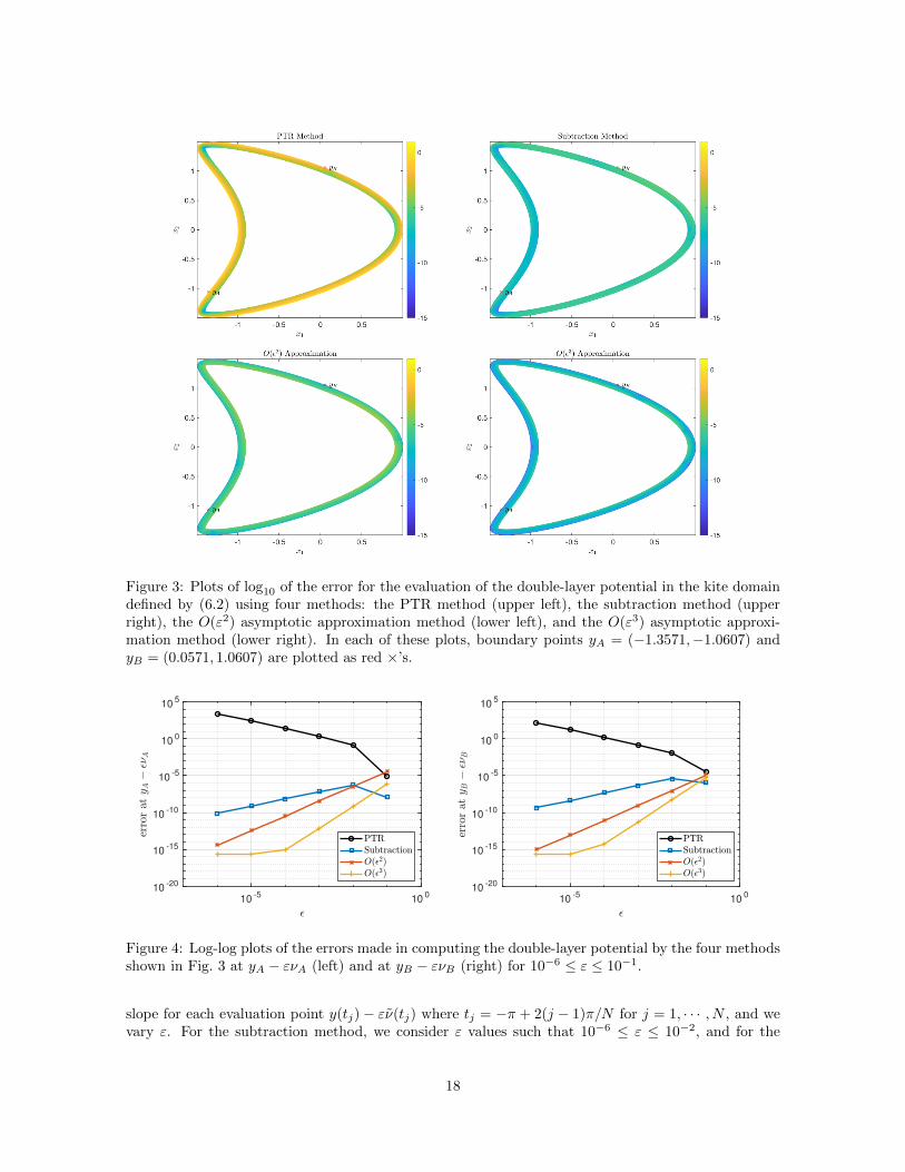
Figure 3: Plots of log10 of the error for the evaluation of the double-layer potential in the kite domaindefined by (6.2) using four methods: the PTR method (upper left), the subtraction method (upperright), the O(ε2) asymptotic approximation method (lower left), and the O(ε3) asymptotic approxi-mation method (lower right). In each of these plots, boundary points yA = (−1.3571,−1.0607) andyB = (0.0571, 1.0607) are plotted as red ×’s.

10-5

100

10-20

10-15

10-10

10-5

100

105

10-5

100

10-20

10-15

10-10

10-5

100

105

Figure 4: Log-log plots of the errors made in computing the double-layer potential by the four methodsshown in Fig. 3 at yA − ενA (left) and at yB − ενB (right) for 10−6 ≤ ε ≤ 10−1.

slope for each evaluation point y(tj)− εν(tj) where tj = −π + 2(j − 1)π/N for j = 1, · · · , N , and wevary ε. For the subtraction method, we consider ε values such that 10−6 ≤ ε ≤ 10−2, and for the

18

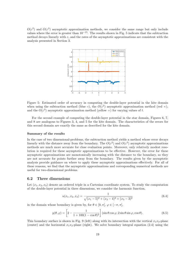
O(ε2) and O(ε3) asymptotic approximation methods, we consider the same range but only includevalues where the error is greater than 10−15. The results shown in Fig. 5 indicate that the subtractionmethod decays linearly with ε, and the rates of the asymptotic approximations are consistent with theanalysis presented in Section 3.

-4 -3 -2 -1 0 1 2 3 4

0

0.5

1

1.5

2

2.5

3

3.5

4

Figure 5: Estimated order of accuracy in computing the double-layer potential in the kite domainwhen using the subtraction method (blue ◦), the O(ε2) asymptotic approximation method (red ×),and the O(ε3) asymptotic approximation method (yellow +) for varying values of t.

For the second example of computing the double-layer potential in the star domain, Figures 6, 7,and 8 are analogous to Figures 3, 4, and 5 for the kite domain. The characteristics of the errors forthis second domain are exactly the same as described for the kite domain.

Summary of the results

In the case of two dimensional-problems, the subtraction method yields a method whose error decayslinearly with the distance away from the boundary. The O(ε2) and O(ε3) asymptotic approximationsmethods are much more accurate for close evaluation points. Moreover, only relatively modest reso-lution is required for these asymptotic approximations to be effective. However, the error for theseasymptotic approximations are monotonically increasing with the distance to the boundary, so theyare not accurate for points further away from the boundary. The results given by the asymptoticanalysis provide guidance on where to apply these asymptotic approximations effectively. For all ofthese reasons, we find that the asymptotic approximations and corresponding numerical methods areuseful for two-dimensional problems.

6.2 Three dimensions

Let (x1, x2, x3) denote an ordered triple in a Cartesian coordinate system. To study the computationof the double-layer potential in three dimensions, we consider the harmonic function,

u(x1, x2, x3) =1√

(x1 − 5)2 + (x2 − 4)2 + (x3 − 3)2(6.4)

in the domain whose boundary is given by, for θ ∈ [0, π], ϕ ∈ [−π, π],

y(θ, ϕ) =

[2− 1

1 + 100(1− cos θ)2

](sin θ cosϕ, 2 sin θ sinϕ, cos θ). (6.5)

This boundary surface is shown in Fig. 9 (left) along with its intersection with the vertical x1x3-plane(center) and the horizontal x1x2-plane (right). We solve boundary integral equation (2.4) using the

19

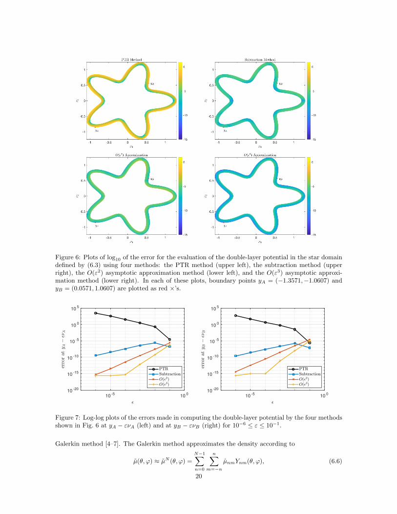
Figure 6: Plots of log10 of the error for the evaluation of the double-layer potential in the star domaindefined by (6.3) using four methods: the PTR method (upper left), the subtraction method (upperright), the O(ε2) asymptotic approximation method (lower left), and the O(ε3) asymptotic approxi-mation method (lower right). In each of these plots, boundary points yA = (−1.3571,−1.0607) andyB = (0.0571, 1.0607) are plotted as red ×’s.

10-5

100

10-20

10-15

10-10

10-5

100

105

10-5

100

10-20

10-15

10-10

10-5

100

105

Figure 7: Log-log plots of the errors made in computing the double-layer potential by the four methodsshown in Fig. 6 at yA − ενA (left) and at yB − ενB (right) for 10−6 ≤ ε ≤ 10−1.

Galerkin method [4–7]. The Galerkin method approximates the density according to

µ(θ, ϕ) ≈ µN (θ, ϕ) =

N−1∑n=0

n∑m=−n

µnmYnm(θ, ϕ), (6.6)

20

-4 -3 -2 -1 0 1 2 3 4

0

0.5

1

1.5

2

2.5

3

3.5

4

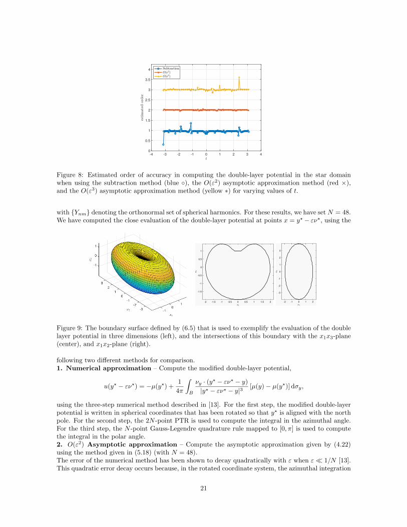
Figure 8: Estimated order of accuracy in computing the double-layer potential in the star domainwhen using the subtraction method (blue ◦), the O(ε2) asymptotic approximation method (red ×),and the O(ε3) asymptotic approximation method (yellow ∗) for varying values of t.

with {Ynm} denoting the orthonormal set of spherical harmonics. For these results, we have set N = 48.We have computed the close evaluation of the double-layer potential at points x = y?− εν?, using the

-2 -1.5 -1 -0.5 0 0.5 1 1.5 2

-1.5

-1

-0.5

0

0.5

1

-2 -1 0 1 2

-3

-2

-1

0

1

2

3

Figure 9: The boundary surface defined by (6.5) that is used to exemplify the evaluation of the doublelayer potential in three dimensions (left), and the intersections of this boundary with the x1x3-plane(center), and x1x2-plane (right).

following two different methods for comparison.1. Numerical approximation – Compute the modified double-layer potential,

u(y? − εν?) = −µ(y?) +1

4π

∫B

νy · (y? − εν? − y)

|y? − εν? − y|3[µ(y)− µ(y?)] dσy,

using the three-step numerical method described in [13]. For the first step, the modified double-layerpotential is written in spherical coordinates that has been rotated so that y? is aligned with the northpole. For the second step, the 2N -point PTR is used to compute the integral in the azimuthal angle.For the third step, the N -point Gauss-Legendre quadrature rule mapped to [0, π] is used to computethe integral in the polar angle.2. O(ε2) Asymptotic approximation – Compute the asymptotic approximation given by (4.22)using the method given in (5.18) (with N = 48).The error of the numerical method has been shown to decay quadratically with ε when ε� 1/N [13].This quadratic error decay occurs because, in the rotated coordinate system, the azimuthal integration

21

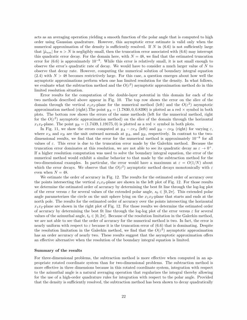
acts as an averaging operation yielding a smooth function of the polar angle that is computed to highorder using Gaussian quadrature. However, this asymptotic error estimate is valid only when thenumerical approximation of the density is sufficiently resolved. If N in (6.6) is not sufficiently largethat |µnm| for n > N is negligibly small, then the truncation error associated with (6.6) may interruptthis quadratic error decay. For the domain here, with N = 48, we find that the estimated truncationerror for (6.6) is approximately 10−8. While this error is relatively small, it is not small enough toobserve the error’s quadratic rate of decay. We would have to consider a much larger value of N toobserve that decay rate. However, computing the numerical solution of boundary integral equation(2.4) with N > 48 becomes restrictively large. For this case, a question emerges about how well theasymptotic approximations perform when one has limited resolution for the density. In what follows,we evaluate what the subtraction method and the O(ε2) asymptotic approximation method do in thislimited resolution situation.

Error results for the computation of the double-layer potential in this domain for each of thetwo methods described above appear in Fig. 10. The top row shows the error on the slice of thedomain through the vertical x1x3-plane for the numerical method (left) and the O(ε2) asymptoticapproximation method (right).The point yA = (1.7830, 0, 0.8390) is plotted as a red × symbol in bothplots. The bottom row shows the errors of the same methods (left for the numerical method, rightfor the O(ε2) asymptotic approximation method) on the slice of the domain through the horizontalx1x2-plane. The point yB = (1.7439, 1.19175, 0) is plotted as a red × symbol in both plots.

In Fig. 11, we show the errors computed at yA − ενA (left) and yB − ενB (right) for varying ε,where νA and νB are the unit outward normals at yA, and yB , respectively. In contrast to the two-dimensional results, we find that the error for the numerical method is approximately 10−8 for allvalues of ε. This error is due to the truncation error made by the Galerkin method. Because thetruncation error dominates at this resolution, we are not able to see its quadratic decay as ε → 0+.If a higher resolution computation was used to solve the boundary integral equation, the error of thenumerical method would exhibit a similar behavior to that made by the subtraction method for thetwo-dimensional examples. In particular, the error would have a maximum at ε = O(1/N) aboutwhich the error decays. We observe that the O(ε2) asymptotic method decays monotonically with εeven when N = 48.

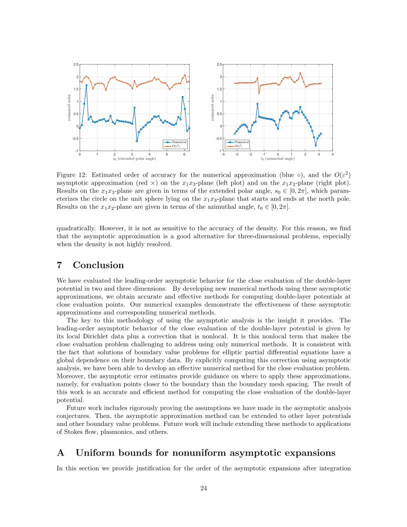
We estimate the order of accuracy in Fig. 12. The results for the estimated order of accuracy overthe points intersecting the vertical x1x3-plane are shown in the left plot of Fig. 12. For those resultswe determine the estimated order of accuracy by determining the best fit line through the log-log plotof the error versus ε for several values of the extended polar angle, s0 ∈ [0, 2π]. This extended polarangle parameterizes the circle on the unit sphere lying on the x1x3-plane that starts and ends at thenorth pole. The results for the estimated order of accuracy over the points intersecting the horizontalx1x2-plane are shown in the right plot of Fig. 12. For those results we determine the estimated orderof accuracy by determining the best fit line through the log-log plot of the error versus ε for severalvalues of the azimuthal angle, t0 ∈ [0, 2π]. Because of the resolution limitation in the Galerkin method,we are not able to see that the order of accuracy for the numerical method is two. In fact, the error isnearly uniform with respect to ε because it is the truncation error of (6.6) that is dominating. Despitethe resolution limitation in the Galerkin method, we find that the O(ε2) asymptotic approximationhas an order accuracy of nearly two. These results suggest that the asymptotic approximation offersan effective alternative when the resolution of the boundary integral equation is limited.

Summary of the results

For three-dimensional problems, the subtraction method is more effective when computed in an ap-propriate rotated coordinate system than for two-dimensional problems. The subtraction method ismore effective in three dimensions because in this rotated coordinate system, integration with respectto the azimuthal angle is a natural averaging operation that regularizes the integral thereby allowingfor the use of a high-order quadrature rules for integration with respect to the polar angle. Providedthat the density is sufficiently resolved, the subtraction method has been shown to decay quadratically

22

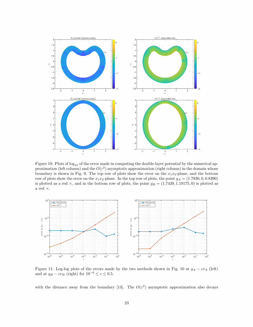
Figure 10: Plots of log10 of the error made in computing the double-layer potential by the numerical ap-proximation (left column) and the O(ε2) asymptotic approximation (right column) in the domain whoseboundary is shown in Fig. 9. The top row of plots show the error on the x1x3-plane, and the bottomrow of plots show the error on the x1x2-plane. In the top row of plots, the point yA = (1.7830, 0, 0.8390)is plotted as a red ×, and in the bottom row of plots, the point yB = (1.7439, 1.19175, 0) is plotted asa red ×.

10-6

10-5

10-4

10-3

10-2

10-1

100

10-15

10-10

10-5

100

10-6

10-5

10-4

10-3

10-2

10-1

100

10-15

10-10

10-5

100

Figure 11: Log-log plots of the errors made by the two methods shown in Fig. 10 at yA − ενA (left)and at yB − ενB (right) for 10−6 ≤ ε ≤ 0.5.

with the distance away from the boundary [13]. The O(ε2) asymptotic approximation also decays

23

0 1 2 3 4 5 6

-1

-0.5

0

0.5

1

1.5

2

2.5

-4 -3 -2 -1 0 1 2 3 4

-1

-0.5

0

0.5

1

1.5

2

2.5

Figure 12: Estimated order of accuracy for the numerical approximation (blue ◦), and the O(ε2)asymptotic approximation (red ×) on the x1x3-plane (left plot) and on the x1x2-plane (right plot).Results on the x1x3-plane are given in terms of the extended polar angle, s0 ∈ [0, 2π], which param-eterizes the circle on the unit sphere lying on the x1x3-plane that starts and ends at the north pole.Results on the x1x2-plane are given in terms of the azimuthal angle, t0 ∈ [0, 2π].

quadratically. However, it is not as sensitive to the accuracy of the density. For this reason, we findthat the asymptotic approximation is a good alternative for three-dimensional problems, especiallywhen the density is not highly resolved.

7 Conclusion

We have evaluated the leading-order asymptotic behavior for the close evaluation of the double-layerpotential in two and three dimensions. By developing new numerical methods using these asymptoticapproximations, we obtain accurate and effective methods for computing double-layer potentials atclose evaluation points. Our numerical examples demonstrate the effectiveness of these asymptoticapproximations and corresponding numerical methods.

The key to this methodology of using the asymptotic analysis is the insight it provides. Theleading-order asymptotic behavior of the close evaluation of the double-layer potential is given byits local Dirichlet data plus a correction that is nonlocal. It is this nonlocal term that makes theclose evaluation problem challenging to address using only numerical methods. It is consistent withthe fact that solutions of boundary value problems for elliptic partial differential equations have aglobal dependence on their boundary data. By explicitly computing this correction using asymptoticanalysis, we have been able to develop an effective numerical method for the close evaluation problem.Moreover, the asymptotic error estimates provide guidance on where to apply these approximations,namely, for evaluation points closer to the boundary than the boundary mesh spacing. The result ofthis work is an accurate and efficient method for computing the close evaluation of the double-layerpotential.

Future work includes rigorously proving the assumptions we have made in the asymptotic analysisconjectures. Then, the asymptotic approximation method can be extended to other layer potentialsand other boundary value problems. Future work will include extending these methods to applicationsof Stokes flow, plasmonics, and others.

A Uniform bounds for nonuniform asymptotic expansions

In this section we provide justification for the order of the asymptotic expansions after integration

24

for (3.8), (3.15), (4.12), (4.19). Throughout the paper we assume that the general boundary B is ananalytic closed boundary that can be mapped to Sn−1, n = 2, 3 (with an analytic diffeomorphism).Therefore, we establish the result for the unit circle (where calculations are explicit), and for theintegrand of (3.5). To obtain (3.15), (4.12), (4.19) one proceeds similarly. One can check that in thiscase the integrand of (3.5) becomes:

F (t; ε) =`(ε`− 2)

2

1

2 + ε`(ε`− 2) + 2(ε`− 1) cos(t)(µ(t)− µ(0)), (A.1)

with the abuse of notation µ(t) = µ(y(t)).

Lemma A.1 (Nonuniform expansion with uniform bounds on the unit circle).

∫ √ε−√ε

F (t; ε)dt =∫ 1/√ε

−1/√ε

εF (εT ; ε)dT =

N∑k=0

εkak + O(εN ), for F given by (A.1), with (ak)k depending on µ and its

derivatives at 0.

Proof. The proof is divided in three steps.

Step 1: Write F (εT ; ε) =N∑

k=−1εkFk(T ) + O(εN+1) and provide an explicit expression for

Fk(T ). We define G(t; ε) := 2 + ε`(ε` − 2) + 2(ε` − 1) cos(t). By substituting t = εT and expandingabout ε = 0 we get

G(εT ; ε) = 2 + ε2`2 − 2ε`+ 2(ε`− 1)

[1− ε2T 2

2+ε4T 4

4!+ ...

],

= ε2(`2 + T 2)

[1− ε `T 2

`2 + T 2+ ε2P (ε, T )

],

where P (ε, T ) is a polynomial in ε and a sum of rational functions in T . Then, after expanding andrearranging the terms we have

1

G(εT ; ε)=

1

ε2(`2 + T 2)

[1 +

N∑m=1

[−ε `T 2

`2 + T 2+ ε2P (ε, T )

]m],

=1

ε21

(`2 + T 2)+

N−2∑m=−1

εmPm(T ) + ...

where Pm(T ) =

2m+4∑j=m+1

αjTj

(`2+T 2)m+3 , with αj ∈ R, j ∈ N polynomial coefficients. From here on after we will

still denote αj while the value can change after each operation.Plugging this expansion into F and expanding the density, µ(t), we obtain, again after combiningterms

F (εT ; ε) =`(ε`− 2)

2

[1

ε21

(`2 + T 2)+

N−2∑m=−1

εmPm(T ) + ...

][N∑k=1

εkT kµ(k)(0) + . . .

]

= − `Tµ′(0)

ε(`2 + T 2)+

N∑k=0

εkFk(T ) +O(εN+1) =

N∑k=−1

εkFk(T ) +O(εN+1),

with Fk(T ) =

3(k+1)∑j=k+1

αj(µ)Tj

(`2+T 2)k+2 , k ≥ 2, and αj(µ) ∈ R coefficients depending on µ and its derivatives at 0.

F0 and F1 can be found in the Mathematica notebook [19].

Step 2: Prove that

∫ 1/√ε

−1/√ε

εk+1Fk(T )dT = O(εk), for all k ≥ 0. One can check that

∫ 1/√ε

−1/√ε

F−1(T )dT =

25

0, and a straightforward computation gives that

∫ 1/√ε

−1/√ε

εk+1Fk(T )dT = O(εk), k = 0, 1. Details of

calculations can be found in the Mathematica notebook [19]. Note that some of the integrals aretreated as a Cauchy principal value. For k ≥ 2, one has

|Fk(T )| ≤3(k+1)∑j=k+1

|αj(µ)|T j−2k−4 ≤k−1∑

j=−k−3

|αj(µ)|T j .

It follows that∣∣∣∣∣∫ 1/

√ε

−1/√ε

εk+1Fk(T )dT

∣∣∣∣∣ ≤2k+3∑j=1

|αj(µ)|ε2k+1−j

2 ≤Mkεk, Mk = 2(k + 1) max

j∈J1,2k+3K|αj(µ)|,

leading to

∫ 1/√ε

−1/√ε

εk+1Fk(T )dT = O(εk), for all k ≥ 0.

Step 3: Establish uniform convergence. We have∫ √ε−√ε

F (t; ε)dt =

∫ 1/√ε

−1/√ε

εF (εT ; ε)dT =

∫ 1/√ε

−1/√ε

(N∑k=0

εk+1F k(T ) +O(εN+2)

)dT.

Using Tonelli’s theorem it follows that∣∣∣∣∣∫ 1/

√ε

−1/√ε

εF (εT ; ε)−N∑k=0

εk+1F k(T )dT

∣∣∣∣∣ =

∣∣∣∣∣∫ 1/

√ε

−1/√ε

( ∞∑k=N+1

εk+1F k(T )

)dT

∣∣∣∣∣ ,≤

∞∑k=N+1

∣∣∣∣∣∫ 1/

√ε

−1/√ε

εk+1F k(T )dT

∣∣∣∣∣ ≤∞∑

k=N+1

Mkεk ≤MN+1ε

N+1

(1 +

∞∑k=1

Mkεk

),

leading to

∫ 1/√ε

−1/√ε

(εF (εT ; ε)−

N∑k=0

εk+1F k(T )

)dT = O(εN+1).

B Rotations on the sphere

We give the explicit rotation formulas over the sphere used in the numerical method for the asymptoticapproximation in three dimensions. Consider y, y? ∈ S2. We introduce the parameters θ ∈ [0, π] andϕ ∈ [−π, π] and write

y = y(θ, ϕ) = sin θ cosϕ ı + sin θ sinϕ + cos θ k. (B.1)

The parameter values, θ? and ϕ?, are set such that that y? = y(θ?, ϕ?). We would like to work in therotated, uvw-coordinate system in which

u = cos θ? cosϕ? ı + cos θ? sinϕ? − sin θ? k,

v = − sinϕ? ı + cosϕ? ,

w = sin θ? cosϕ? ı + sin θ? sinϕ? + cos θ? k.

(B.2)

Notice that w = y?. For this rotated coordinate system, we introduce the parameters s ∈ [0, π] andt ∈ [−π, π] such that

y = y(s, t) = sin s cos t u + sin s sin t v + cos s w. (B.3)

26

It follows that y? = y(0, ·). By equating (B.1) and (B.3) and substituting (B.2) into that result, weobtain sin θ cosϕ

sin θ sinϕcos θ

=

cos θ? cosϕ? − sinϕ? sin θ? cosϕ?

cos θ? sinϕ? cosϕ? sin θ? sinϕ?

− sin θ? 0 cos θ?

sin s cos tsin s sin t

cos s

. (B.4)

We rewrite (B.4) compactly as y(θ, ϕ) = R(θ?, ϕ?)y(s, t) with R(θ?, ϕ?) denoting the 3× 3 orthogonalrotation matrix. We now seek to write θ = θ(s, t) and ϕ = ϕ(s, t). To do so, we introduce

ξ(s, t; θ?, ϕ?) = cos θ? cosϕ? sin s cos t− sinϕ? sin s sin t+ sin θ? cosϕ? cos s, (B.5)

η(s, t, θ?, ϕ?) = cos θ? sinϕ? sin s cos t+ cosϕ? sin s sin t+ sin θ? sinϕ? cos s, (B.6)

ζ(s, t, θ?, ϕ?) = − sin θ? sin s cos t+ cos θ? cos s. (B.7)

From (B.4), we find that

θ = arctan

(√ξ2 + η2

ζ

), and ϕ = arctan

(η

ξ

). (B.8)

With these formulas, we can write θ = θ(s, t) and ϕ = ϕ(s, t).

C Spherical Laplacian

In this Appendix, we establish the result given in (4.10). We first seek an expression for ∂2s [·]|s=0 interms of θ and ϕ. By the chain rule, we find that

∂2

∂s2[·]∣∣∣∣s=0

=

[(∂θ

∂s

)2∂2

∂θ2+

(∂ϕ

∂s

)2∂2

∂ϕ2+ 2

∂θ

∂s

∂ϕ

∂s

∂2

∂θ∂ϕ+∂2θ

∂s2∂

∂θ+∂2ϕ

∂s2∂

∂ϕ

] ∣∣∣∣s=0

. (C.1)

Using θ and ϕ defined in (B.8), we find that

∂θ(s, t)

∂s

∣∣∣∣s=0

= cos t,∂2θ(s, t)

∂s2

∣∣∣∣s=0

=cos θ?

sin θ?sin2 t, (C.2)

∂ϕ(s, t)

∂s

∣∣∣∣s=0

=sin t

sin θ?,

∂2ϕ(s, t)

∂s2

∣∣∣∣s=0

= − cos θ?

sin2 θ?sin 2t. (C.3)

Note that at s = 0, we have θ? = θ. Substituting (C.2) – (C.3) into (C.1) and replacing θ? by θ, weobtain

∂2

∂s2[·]∣∣∣∣s=0

= cos2 t∂2

∂θ2+ sin2 t

1

sin2 θ

∂2

∂ϕ2+ 2 cos t sin t

1

sin θ

∂2

∂θ∂ϕ

+ sin2 tcos θ

sin θ

∂

∂θ− sin 2t

cos θ

sin2 θ

∂

∂ϕ, (C.4)

from which it follows that

1

π

∫ π

0

∂2

∂s2[·]∣∣∣∣s=0

dt =1

2

[∂2

∂θ2+

cos θ

sin θ

∂

∂θ+

1

sin2 θ

∂2

∂ϕ2

]=

1

2∆S2 . (C.5)

which establishes the result.

27

References

[1] L. af Klinteberg and A.-K. Tornberg, A fast integral equation method for solid particles inviscous flow using quadrature by expansion, J. Comput. Phys., 326 (2016), pp. 420–445.

[2] L. af Klinteberg and A.-K. Tornberg, Error estimation for quadrature by expansion inlayer potential evaluation, Adv. Comput. Math., 43 (2017), pp. 195–234.

[3] G. M. Akselrod, C. Argyropoulos, T. B. Hoang, C. Ciracı, C. Fang, J. Huang,D. R. Smith, and M. H. Mikkelsen, Probing the mechanisms of large Purcell enhancement inplasmonic nanoantennas, Nat. Photonics, 8 (2014), pp. 835–840.

[4] K. E. Atkinson, The numerical solution Laplace’s equation in three dimensions, SIAM J. Numer.Anal., 19 (1982), pp. 263–274.

[5] K. E. Atkinson, Algorithm 629: An integral equation program for Laplace’s equation in threedimensions, ACM Trans. Math. Softw., 11 (1985), pp. 85–96.

[6] K. E. Atkinson, A survey of boundary integral equation methods for the numerical solution ofLaplace’s equation in three dimensions, in Numerical Solution of Integral Equations, Springer,1990, pp. 1–34.

[7] K. E. Atkinson, The Numerical Solution of Integral Equations of the Second Kind, CambridgeUniversity Press, 1997.

[8] A. Barnett, B. Wu, and S. Veerapaneni, Spectrally accurate quadratures for evaluationof layer potentials close to the boundary for the 2d Stokes and Laplace equations, SIAM J. Sci.Comput., 37 (2015), pp. B519–B542.

[9] A. H. Barnett, Evaluation of layer potentials close to the boundary for Laplace and Helmholtzproblems on analytic planar domains, SIAM J. Sci. Comput., 36 (2014), pp. A427–A451.

[10] J. T. Beale and M.-C. Lai, A method for computing nearly singular integrals, SIAM J. Numer.Anal., 38 (2001), pp. 1902–1925.

[11] J. T. Beale, W. Ying, and J. R. Wilson, A simple method for computing singular or nearlysingular integrals on closed surfaces, Commun. Comput. Phys., 20 (2016), pp. 733–753.

[12] C. Carvalho, S. Khatri, and A. D. Kim, Asymptotic analysis for close evaluation of layerpotentials, J. Comput. Phys., 355 (2018), pp. 327–341.

[13] C. Carvalho, S. Khatri, and A. D. Kim, Close evaluation of layer potentials in three dimen-sions, arXiv:1807.02474, (2018).

[14] C. L. Epstein, L. Greengard, and A. Klockner, On the convergence of local expansions oflayer potentials, SIAM J. Numer. Anal., 51 (2013), pp. 2660–2679.

[15] R. B. Guenther and J. W. Lee, Partial Differential Equations of Mathematical Physics andIntegral Equations, Dover Publications, 1996.

[16] J. Helsing and R. Ojala, On the evaluation of layer potentials close to their sources, J. Comput.Phys., 227 (2008), pp. 2899–2921.

[17] E. J. Hinch, Perturbation Methods, Cambridge University Press, 1991.

[18] E. E. Keaveny and M. J. Shelley, Applying a second-kind boundary integral equation forsurface tractions in Stokes flow, J. Comput. Phys., 230 (2011), pp. 2141–2159.

[19] A. D. Kim, Asymptotic-DLP. https://github.com/arnolddkim/Asymptotic-DLP, 2018.

28

[20] A. Klockner, A. Barnett, L. Greengard, and M. O’Neil, Quadrature by expansion: Anew method for the evaluation of layer potentials, J. Comput. Phys., 252 (2013), pp. 332–349.

[21] R. Kress, Linear Integral Equations, Springer-Verlag, New York, 1999.

[22] S. A. Maier, Plasmonics: Fundamentals and Applications, Springer, 2007.

[23] G. R. Marple, A. Barnett, A. Gillman, and S. Veerapaneni, A fast algorithm for simu-lating multiphase flows through periodic geometries of arbitrary shape, SIAM J. Sci. Comput., 38(2016), pp. B740–B772.

[24] K. M. Mayer, S. Lee, H. Liao, B. C. Rostro, A. Fuentes, P. T. Scully, C. L. Nehl,and J. H. Hafner, A label-free immunoassay based upon localized surface plasmon resonance ofgold nanorods, ACS Nano, 2 (2008), pp. 687–692.

[25] P. Miller, Applied Asymptotic Analysis, American Mathematical Soc., 2006.

[26] L. Novotny and N. Van Hulst, Antennas for light, Nat. Photonics, 5 (2011), pp. 83–90.

[27] M. Rachh, A. Klockner, and M. O’Neil, Fast algorithms for quadrature by expansion i:Globally valid expansions, J. Comput. Phys., 345 (2017), pp. 706–731.

[28] T. Sannomiya, C. Hafner, and J. Voros, In situ sensing of single binding events by localizedsurface plasmon resonance, Nano Lett., 8 (2008), pp. 3450–3455.

[29] C. Schwab and W. Wendland, On the extraction technique in boundary integral equations,Math. Comput., 68 (1999), pp. 91–122.

[30] D. J. Smith, A boundary element regularized Stokeslet method applied to cilia-and flagella-drivenflow, Proc. R. Soc. Lond. A, 465 (2009), pp. 3605–3626.

[31] M. Wala and A. Klockner, A fast algorithm for Quadrature by Expansion in three dimensions,Journal of Computational Physics, 388 (2019), pp. 655–689.

29