Asymptotic Approximations of the Stable and Unstable Manifolds …campus.mst.edu/ijde/contents/v10n1p3.pdf · 2015-05-01 · Asymptotic Approximations of the Stable and Unstable Manifolds

International Journal of Difference EquationsISSN 0973-6069, Volume 10, Number 1, pp. 39–58 (2015)http://campus.mst.edu/ijde

Asymptotic Approximations of theStable and Unstable Manifolds of Fixed Points

of a Two-dimensional Cubic Map

Jasmin BektesevicUniversity of Sarajevo

Faculty of Mechanical EngineeringSarajevo, 71000, Bosnia and Herzegovina

[email protected]

Mustafa R. S. KulenovicUniversity of Rhode IslandDepartment of Mathematics

Kingston, Rhode Island 02881-0816, [email protected]

Esmir PilavUniversity of Sarajevo

Department of MathematicsSarajevo, 71000, Bosnia and Herzegovina

[email protected]

Abstract

We find the asymptotic approximations of the stable and unstable manifolds ofthe saddle equilibrium solutions of the following difference equation xn+1 =ax3n + bx3n−1 + cxn + dxn−1, n = 0, 1, . . . where the parameters a, b, c and dare positive numbers and the initial conditions x−1 and x0 are arbitrary numbers.These manifolds determine completely the global dynamics of this equation.

Keywords: 39A10, 39A11, 37E99, 37D10.AMS Subject Classifications: Basin of attraction, cooperative map, normal form, sta-ble manifold, unstable manifold, monotonicity.

Received January 10, 2015; Accepted March 29, 2015Communicated by Martin Bohner

40 J. Bektesevic, M. R. S. Kulenovic and E. Pilav

1 IntroductionIn this paper we consider the difference equation

xn+1 = ax3n + bx3n−1 + cxn + dxn−1, (1.1)

where the parameters a, b, c and d are positive numbers and the initial conditions x−1and x0 are arbitrary numbers. Equation (1.1) is a special case of a general second or-der difference equation with cubic terms considered in [2], where the global dynamicswas established in the case of all non-negative parameters and the initial conditions, inthe hyperbolic case. In [2] we found precisely the basins of attraction of all attractors,which are either equilibrium points, period-two solutions or the point at infinity. Theboundaries of these basins of attraction are the global stable manifolds of neighboringsaddle equilibrium points (resp. nonhyperbolic equilibrium points of stable type) or thesaddle period-two points (resp. nonhyperbolic period-two points of stable type). Theunstable manifolds of neighboring saddle equilibrium points (resp. nonhyperbolic equi-librium points of stable type) play the role of carrying simplex, that is of the manifoldwhich eventually carries the solutions toward its attractor. See [1] for similar results onsecond order difference equation with quadratic terms.

In this paper we demonstrate the computational procedure for finding the local stableand unstable manifold for equation (1.1). The method can be extended in a straightfor-ward manner to the general second order difference equation with cubic terms consid-ered in [2], but it will be computationally extensive and it will contain 10 parameters.

The paper is organized as follows. The rest of this section contains the result onglobal behavior of solutions of equation (1.1) from [2]. Section 2 contains some prelim-inary results about cooperative maps needed to establish the smoothness of stable andunstable manifolds and so justify the use of a method of undetermined coefficients. Sec-tion 3 contains a computational procedure and asymptotic expansions of two invariantmanifolds, obtained by using Mathematica. Finally Section 4 contains some numericalexamples and the comparison of the asymptotic expansions of global stable manifoldswith the basins of attraction obtained by Dynamica 3 [7]. Appendix gives the valuesof some coefficients in asymptotic expansions of two invariant manifolds, obtained byusing Mathematica.

Setun = xn−1 and vn = xn for n = 0, 1, . . . (1.2)

and write Eq.(1.1) in the equivalent form:

un+1 = vn (1.3)vn+1 = av3n + bu3n + cvn + dun.

Let T be the corresponding map defined by:

T

(uv

)=

(v

av3 + bu3 + cv + du

). (1.4)

Asymptotic Approximations of the Stable and Unstable Manifolds 41

The following result was established in [2]:

Theorem 1.1. If

c+ d < 1 and((

c >(d− 1)(2a− b)

2b− aand 2a < b

)or 2a ≥ b

)(1.5)

then Eq.(1.1) has three distinct equilibrium points x− = −√

1− c− d√a+ b

, x0 = 0 and

x+ =

√1− c− d√a+ b

, and the following holds:

i) x− and x+ are the saddle points;

ii) x0 is locally asymptotically stable.

Further, there exist four continuous curves Ws(x−),Ws(x+) (stable manifolds of x−and x+), Wu(x−),Wu(x+), (unstable manifolds of x− and x−) where Ws(x−) andWs(x+) are passing through the points E−(x−, x−) and E+(x+, x+) respectively, andare graphs of decreasing functions. The curves Wu(x−) are the graphs of increasingfunctions, and it has endpoints E−(x−, x−) and E0(0, 0). The curve Wu(x+) is thegraphs of increasing function and it has the endpoints E0(0, 0) and E+(x+, x+). Everysolution {xn} which starts below Ws(x+) and above Ws(x−) in North-east orderingconverges to E0(0, 0) and every solution {xn} which starts above Ws(x+) or belowWs(x−) in North-east ordering satisfies limxn =∞. The set of initial conditions R2 isthe union of four disjoint basins of attraction, namely

R2 = B(E−) ∪ B(E+) ∪ B(E) ∪ B(E∞),

where E−, E, E+and E∞ denote the points (x−, x−), (0, 0), (x+, x+) and (∞,∞)respectively, and

B(E−) =Ws(E−),

B(E+) =Ws(E+),

B(E0) ={

(x, y)|(xE− , yE−) �ne (x, y) �ne (xE+ , yE+) for some

(xE+ , yE+) ∈ Ws(E+) and (xE− , yE−) ∈ Ws(E−)},

B(E∞) ={

(x, y)|(xE+ , yE+) �ne (x, y) for some (xE+ , yE+) ∈ Ws(E+)}

∪{

(x, y)|(x, y) �ne (xE− , yE−) for some (xE− , yE−) ∈ Ws(E−)}.

As one may see from Theorem 1.1 the boundaries of the basins of attraction of all at-tractors of Eq.(1.1) are the stable manifolds of equilibrium points. In addition, by usingthe results from [10] one can see that the solutions which are asymptotic to the locallyasymptotically stable equilibrium solutions are approaching the unstable manifolds ofthe neighboring saddle equilibrium points. The monotonicity and smoothness of stable


and unstable manifolds for the map T given with (1.4) is guaranteed by Theorems 2.1,2.3, 2.4 of [10]. See [5, 8, 10, 13, 14] for related results about the stable manifolds forcompetitive maps. Our main goal here is to get the local asymptotic estimates for thesemanifolds for both equilibrium solutions. We will bring the considered map to the nor-mal form around the equilibrium solutions and then use the method of undeterminedcoefficients to find the local approximations of the considered manifolds. Since the mapT is cooperative, it is guaranteed that both stable and unstable manifolds are as smoothas the functions of the considered map and that are monotonic such that the stable man-ifold is decreasing and unstable manifold is increasing, see [3, 10]. See [5, 11, 15] forsimilar local approximations of stable and unstable manifolds. See [4, 6, 7, 12, 15] forbasic results on stable and unstable manifolds for general maps.

2 PreliminariesIn this section we present some basic results for the cooperative maps which describethe existence and the properties of their invariant manifolds.

A first order system of difference equations{xn+1 = f(xn, yn)yn+1 = g(xn, yn)

, n = 0, 1, 2, . . . , (x0, y0) ∈ S , (2.1)

where S ⊂ R2, (f, g) : S → S, f , g are continuous functions is cooperative if f(x, y)and g(x, y) are non-decreasing in x and y. Strongly cooperative systems of differenceequations or strongly cooperative maps are those for which the functions f and g arecoordinate-wise strictly monotone.

If v = (u, v) ∈ R2, we denote with Q`(v), ` ∈ {1, 2, 3, 4}, the four quadrants inR2 relative to v, i.e., Q1(v) = {(x, y) ∈ R2 : x ≥ u, y ≥ v}, Q2(v) = {(x, y) ∈R2 : x ≤ u, y ≥ v}, and so on. Define the South-East partial order �se on R2 by(x, y) �se (s, t) if and only if x ≤ s and y ≥ t. Similarly, we define the North-Eastpartial order �ne on R2 by (x, y) �ne (s, t) if and only if x ≤ s and y ≤ t. For A ⊂ R2

and x ∈ R2, define the distance from x to A as dist(x,A) := inf {‖x − y‖ : y ∈ A}.By intA we denote the interior of a set A.

It is easy to show that a map F is cooperative if it is non-decreasing with respect tothe North-East partial order, that is if the following holds:(

x1

y1

)�ne

(x2

y2

)⇒ F

(x1

y1

)�ne F

(x2

y2

). (2.2)

The following five results were proved by Kulenovic and Merino [10] for compet-itive systems in the plane, when one of the eigenvalues of the linearized system at anequilibrium (hyperbolic or non-hyperbolic) is by absolute value smaller than 1 while theother has an arbitrary value. We give the analogue versions for cooperative maps.

A regionR ⊂ R2 is rectangular if it is the cartesian product of two intervals in R.


Theorem 2.1. Let T be a cooperative map on a rectangular regionR ⊂ R2. Let x ∈ Rbe a fixed point of T such that ∆ := R ∩ int (Q2(x) ∪ Q4(x)) is nonempty (i.e., x isnot the NE or SW vertex of R), and T is strongly cooperative on ∆. Suppose that thefollowing statements are true.

a. The map T has a C1 extension to a neighborhood of x.

b. The Jacobian matrix of T at x has real eigenvalues λ, µ such that 0 < |λ| < µ,where |λ| < 1, and the eigenspace Eλ associated with λ is not a coordinate axis.

Then there exists a curve C ⊂ R through x that is invariant and a subset of the basinof attraction of x, such that C is tangential to the eigenspace Eλ at x, and C is the graphof a strictly decreasing continuous function of the first coordinate on an interval. Anyendpoints of C in the interior ofR are either fixed points or minimal period-two points.In the latter case, the set of endpoints of C is a minimal period-two orbit of T .

Corollary 2.2. If T has no fixed point nor periodic points of minimal period two in ∆,then the endpoints of C belong to ∂R.

As is well known for maps that are strongly cooperative near the fixed point, hy-pothesis (b). of Theorem 2.1 reduces just to |λ| < 1, see [10]. Also, one can show thatin such a case no associated eigenvector is aligned with a coordinate axis.

Theorem 2.3. Under the hypotheses of Theorem 2.1, suppose there exists a neighbor-hood U of x in R2 such that T is of class Ck on U ∪ ∆ for some k ≥ 1, and thatthe Jacobian of T at each x ∈ ∆ is invertible. Then the curve C in the conclusion ofTheorem 2.1 is of class Ck.

The following result gives a description of the global stable and unstable manifoldsof a saddle point of a cooperative map. The result is the modification of Theorem 5from [8]. See also [9].

Theorem 2.4. In addition to the hypotheses of Theorem 2.1, suppose that µ > 1 andthat the eigenspace Eµ associated with µ is not a coordinate axis. If the curve C ofTheorem 2.1 has endpoints in ∂R, then C is the global stable manifoldWs(x) of x, andthe global unstable manifold Wu(x) is a curve in R that is tangential to Eµ at x andsuch that it is the graph of a strictly increasing function of the first coordinate on aninterval. Any endpoints ofWu(x) inR are fixed points of T .

Theorem 2.5. Assume the hypotheses of Theorem 2.1, and let C be the curve whoseexistence is guaranteed by Theorem 2.1. If the endpoints of C belong to ∂R, then CseparatesR into two connected components, namely

W− : = {x ∈ R \ C : ∃y ∈ C with x �ne y}W+ : = {x ∈ R \ C : ∃y ∈ Cwith y �ne x} ,

(2.3)

such that the following statements are true.


(i) W− is invariant, and dist(T n(x),Q1(x))→ 0 as n→∞ for every x ∈ W−.

(ii) W+ is invariant, and dist(T n(x),Q3(x))→ 0 as n→∞ for every x ∈ W+.

If, in addition, x is an interior point of R and T is C2 and strongly cooperative ina neighborhood of x, then T has no periodic points in the boundary of Q2(x) ∪ Q4(x)except for x, and the following statements are true.

(iii) For every x ∈ W− there exists n0 ∈ N such that T n(x) ∈ intQ1(x) for n ≥ n0.

(iv) For every x ∈ W+ there exists n0 ∈ N such that T n(x) ∈ intQ3(x) for n ≥ n0.

Remark 2.6. The map T defined with (1.4) is strongly cooperative in R2. Theorems2.1, 2.3 and 2.4 show that the stable and unstable manifolds of cooperative maps, whichsatisfies certain conditions, are simple monotonic curves which are as smooth as thefunctions of the map. Thus the assumed forms of these manifolds are justified. As iswell-known the stable and unstable manifolds of general maps can have complicatedstructure consisting of many branches or being strange attractors, see [4,6,15] for someexamples of polynomial maps such as Henon with unstable manifold being a strangeattractor. Finally, see [14] for examples of competitive and so cooperative maps in theplane with chaotic attractors.

3 Invariant Manifolds and Normal FormsLet (

ξn+1

ηn+1

)=

(µ1 00 µ2

)(ξnηn

)+

(g1(ξn, ηn)g2(ξn, ηn)

), (3.1)

where g1(0, 0) = 0, g2(0, 0) = 0, Dg1(0, 0) = 0 and Dg2(0, 0) = 0. Suppose that|µ1| < 1 and |µ2| > 1. Then, there are two unique invariant manifolds Ws and Wu

tangents to (1, 0) and (0, 1) at (0,0), which are graphs of the maps ϕ : E1 → E2 and ψ :E1 → E2, such that ϕ(0) = ψ(0) = 0 and ϕ′(0) = ψ′(0) = 0. See [5,6,11,15]. Lettingηn = ϕ(ξn) yields

ηn+1 = ϕ(ξn+1) = ϕ(µ1ξn + g1(ξn, ϕ(ξn))). (3.2)

On the other hand by (3.1)

ηn+1 = µ2ϕ(ξn) + g2(ξn, ϕ(ξn)). (3.3)

Equating equations (3.2) and (3.3) yields

ϕ(µ1ξn + g1(ξn, ϕ(ξn))) = µ2ϕ(ξn) + g2(ξn, ϕ(ξn)). (3.4)


Similarly, letting ξn = ψ(ηn) yields

ξn+1 = ψ(ηn+1) = ψ(µ2ηn + g2(ψ(ηn), ηn)). (3.5)

By using (3.1) we obtain

ξn+1 = µ1ψ(ηn) + g1(ψ(ηn), ηn). (3.6)

Equating equations (3.5) and (3.6) yields

ψ(µ2ηn + g2(ψ(ηn), ηn)) = µ1ψ(ηn) + g1(ψ(ηn), ηn). (3.7)

Thus the functional equations (3.4) and (3.7), define the local stable manifoldWs ={(ξ, η) ∈ R2 : η = ϕ(ξ)}, and the local unstable manifold Wu = {(ξ, η) ∈ R2 :ξ = ψ(η)}. Without loss generality, we can assume that solutions of the functionalequations (3.4) and (3.7) take the forms ϕ(ξ) = α1ξ

2 + β1ξ3 + O(|ξ|4) and ψ(η) =

α2η2 + β2η

3 +O(|η|4).

3.1 Normal Form of the Map T at the Saddle Points x− and x+

Let x denote one of the saddle points x− or x+. Put yn = xn− x. Then Eq(1.1) becomes

yn+1 = a (x+ yn) 3 + b (x+ yn−1)3 + c (x+ yn) + d (x+ yn−1)− x. (3.8)

Set un = yn−1 and vn = yn for n = 0, 1, . . . and write Eq(3.8) in the equivalent form:

un+1 = vn (3.9)vn+1 = a (x+ vn) 3 + b (x+ un)3 + c (x+ vn) + d (x+ un)− x.

Let F be the function defined by:

F

(uv

)=

(v

a (x+ v) 3 + b (x+ u)3 + c (x+ v) + d (x+ u)− x

). (3.10)

Then F has the fixed point (0, 0), which corresponds to the fixed point (x, x) of the mapT. The Jacobian matrix of F is given by

JacF (u, v) =

(0 1

d+ 3b (u+ x)2 c+ 3a (v + x)2

).

At (0, 0), JacF (u, v) has the form

J0 = JacF (0, 0) =

(0 1

d+ 3bx2 c+ 3ax2

)

=

0 1−3cb− 2db+ 3b+ ad

a+ b

−2ca− 3da+ 3a+ bc

a+ b

.

(3.11)


The eigenvalues of (3.11) are µ1,2 where

µ1 = −a(2c+ 3d− 3)− bc+ A

2(a+ b)and µ2 = −a(2c+ 3d− 3)− bc− A

2(a+ b),

andA =

√(a(−2c− 3d+ 3) + bc)2 + 4(a+ b)(ad+ b(−3c− 2d+ 3)),

and the corresponding eigenvectors are given by

v1 =

(−2ac− 3ad+ 3a+ bc+ A

b(6c+ 4d− 6)− 2ad, 1

)Tand

v2 =

(−2ac− 3ad+ 3a+ bc− Ab(6c+ 4d− 6)− 2ad

, 1

)T,

respectively.Then we have that

F

(uv

)=

(0 1

d+ 3bx2 c+ 3ax2

)(uv

)+

(f1(u, v)g1(u, v)

), (3.12)

and

f1(u, v) =0

g1(u, v) =x(3av2 + 3bu2 − 1 + c+ d

)+ (a+ b)x3 + av3 + bu3.

Then, the system (3.9) is equivalent to(un+1

vn+1

)=

(0 1

d+ 3bx2 c+ 3ax2

)(unvn

)+

(f1(un, vn)g1(un, vn)

). (3.13)

Let (unvn

)= P ·

(ξnηn

)where

P =

−2ca+ 3da− 3a− A− bc2(3cb+ 2db− 3b− ad)

−2ca− 3da+ 3a− A+ bc

2(3cb+ 2db− 3b− ad)1 1

and

P−1 =

3cb+ 2db− 3b− adA

2ca+ 3da− 3a+ A− bc2A

−3cb− 2db+ 3b+ ad

A

−2ca− 3da+ 3a+ A+ bc

2A

.


Then system (3.13) is equivalent to(ξn+1

ηn+1

)=

(µ1 00 µ2

)(ξnηn

)+

(f1(ξn, ηn)g1(ξn, ηn)

), (3.14)

where (f1(u, v)g1(u, v)

):= P−1 ·H1

(P ·(uv

))and

H1

(uv

):=

(f1(u, v)g1(u, v)

).

By straightforward calculation we obtain that

f1(u, v) =a(2c+ 3d− 3) + A− bc

2AΥ1(u, v),

g1(u, v) =a(−2c− 3d+ 3) + A+ bc

2AΥ1(u, v),

where

Υ1(u, v) = x

(3b(−a(2c+ 3d− 3)(u+ v) + A(u− v) + bc(u+ v))2

4(ad+ b(−3c− 2d+ 3))2

)+ x

(3a(u+ v)2 + c+ d− 1

)+ a(u+ v)3

+ x3(a+ b) +b(−a(2c+ 3d− 3)(u+ v) + A(u− v) + bc(u+ v))3

8(b(3c+ 2d− 3)− ad)3.

3.2 Stable Manifolds at x− and x+

Assume that (1.5) holds and that the local stable manifold corresponding to the saddlepoint E+ is the graph of the function ϕ1 of the form

ϕ1(ξ) = α1ξ2 + β1ξ

3 +O(|ξ|4), α1, β1 ∈ R,

and that the local stable manifold corresponding to the saddle point E− is the graph ofthe function ϕ2 of the form

ϕ2(ξ) = α2ξ2 + β2ξ

3 +O(|ξ|4), α2, β2 ∈ R,

Now we compute the constants α1, α2, β1 and β2. The function ϕ1 must satisfy thestable manifold equation

ϕ1

(µ1ξ + f1 (ξ, ϕ1(ξ))

)= µ2ϕ1(ξ) + g1 (ξ, ϕ1(ξ)) ,


for x =

√1− c− d√a+ b

. This leads to the following polynomial equation

p1ξ2 + p2ξ

3 + · · ·+ p26ξ27 = 0.

Substituting x2 into p1 and p2 and solving system p1 = 0 and p2 = 0, we obtain thevalues

α1 =Υ1

Υ2

, β1 =Υ3

Υ4

where the coefficients Υ3 and Υ4, generated by Mathematica are in Appendix A and

Υ1 = 3(a+ b)3/2√

1− c− d(a(2c+ 3d− 3) + A− bc)(4a3d2 + a2b

(4c2 − 12c(d+ 1) + (6− 7d)d+ 9

)+ 2ab (A(2c+ 3d− 3)

+b(16c2 + 3c(7d− 11) + 2(3− 2d)2

))+ b(A− bc)2

),

Υ2 = 2A(ad+ b(3− 3c− 2d))2(a2(2c+ 3d− 3)(2c+ 3d− 1)− 2a(3d(A

+b(c− 1)) + 2(c− 2)(A+ bc) + 3b) + A2 + 2Ab(c+ 1) + b2(c− 2)c).

Since ηn = α1ξ2n + β1ξ

3n, and(

ξnηn

)= P−1 ·

(xn−1 − x+xn − x+

)(3.15)

we can approximate locally the local stable manifoldWsloc(x+, x+) as the graph of the

map ϕ1(x) such that S+(x, ϕ1(x)) = 0 where

S+(x, y) :=(y − x+) (a(3− 2c− 3d) +A+ bc) + 2 (x− x+) (ad+ b(3− 3c− 2d))

2A

− β1 ((A− bc+ a(2c+ 3d− 3)) (y − x+) + (x− x+) (b(6c+ 4d− 6)− 2ad)) 3

8A3

− α1 ((A− bc+ a(2c+ 3d− 3)) (y − x+) + (x− x+) (b(6c+ 4d− 6)− 2ad)) 2

4A3(3.16)

and which satisfies

ϕ1(x+) = x+ and ϕ′1(x+) =b(6c+ 4d− 6)− 2ad

−2ac− 3ad+ 3a+ bc+ A.

The function ϕ2 must satisfy the stable manifold equation

ϕ2

(µ1ξ + f1 (ξ, ϕ2(ξ))

)= µ2ϕ2(ξ) + g1 (ξ, ϕ2(ξ)) ,

for x = −√

1− c− d√a+ b


p′1ξ2 + p′2ξ

3 + · · ·+ p′26ξ27 = 0.


Substituting x2 into p′1 and p′2 and solving system p′1 = 0 and p′2 = 0, we obtain thevalues

α2 = −α1 = −Υ1

Υ2

, β2 =Υ5

Υ4

where the coefficient Υ5, generated by Mathematica is in appendix A. Since ηn =α2ξ

2n + β2ξ

3n, (3.15) we can approximate locally the local stable manifoldWs

loc(x−, x−)as the graph of the map ϕ2(x) such that S−(x, ϕ2(x)) = 0 where

S−(x, y) :=(y − x−) (a(3− 2c− 3d) +A+ bc) + 2 (x− x−) (ad+ b(3− 3c− 2d))

2A

− β2 ((A− bc+ a(2c+ 3d− 3)) (y − x−) + (x− x−) (b(6c+ 4d− 6)− 2ad)) 3

8A3

− α2 ((A− bc+ a(2c+ 3d− 3)) (y − x−) + (x− x−) (b(6c+ 4d− 6)− 2ad)) 2

4A3(3.17)

and which satisfies

ϕ2(x−) = x− and ϕ′2(x−) =b(6c+ 4d− 6)− 2ad

−2ac− 3ad+ 3a+ bc+ A.

Theorem 3.1. Consider Eq.(1.1). Then the local stable manifolds corresponding to thesaddle points x+ and x− are given with the asymptotic expansions S+(x, ϕ1(x)) = 0and S−(x, ϕ2(x)) = 0 respectively.

3.3 Unstable Manifolds at x− and x+

Assume (1.5) and that the local unstable manifold, that corresponds to the saddle point

x+ =

√1− c− d√a+ b

, is the graph of the function ψ1 that has the form

ψ1(η) = γ1η2 + δ1η

3 +O(|η|4), γ1, δ1 ∈ R

and that the local unstable manifold, that corresponds to the saddle point

x− = −√

1− c− d√a+ b

,

is the graph of the function ψ2 that has the form

ψ2(η) = γ2η2 + δ2η

3 +O(|η|4), γ2, δ2 ∈ R.

Now we compute the constants γ1 and δ1.The function ψ1 must satisfy the unstable manifold equation

ψ1(µ2η + g1(ψ1(η), η)) = µ1ψ1(η) + f1(ψ1(η), η),


for x = x+ =

√1− c− d√a+ b


q1η2 + q2η

3 + · · ·+ q26η27 = 0.

Substituting x+ into q1 and q2 and solving system q1 = 0 and q2 = 0, we obtain thevalues

γ1 =Γ1

Γ2

, δ1 =Γ3

Γ4

.

where the coefficients Γ3 and Γ4, generated by Mathematica are in Appendix A and

Γ1 = 3(a+ b)3/2√−c− d+ 1(a(2c+ 3d− 3) +A− bc)

(4a3d2 + a2b

(4c2 − 12c(d+ 1)

+(6− 7d)d+ 9) + 2ab(A(2c+ 3d− 3) + b

(16c2 + 3c(7d− 11) + 2(3− 2d)2

))+b(A− bc)2

)Γ2 = 2A(ad+ b(−3c− 2d+ 3))2

(a2(2c+ 3d− 3)(2c+ 3d− 1)− 2a(3d(A+ b(c− 1))

+2(c− 2)(A+ bc) + 3b) +A2 + 2Ab(c+ 1) + b2(c− 2)c).

Since ξn = γ1η2n + δ1η

3n, and (3.15) we can approximate locally the local unstable

manifoldWuloc(x+, x+) as the graph of the map ψ1(y) such that U(ψ1(y), y) = 0 where

U+(x, y) :=(y − x+) (a(2c+ 3d− 3) +A− bc) + (x− x+) (2ad+ b(6c+ 4d− 6))

2A

− δ1 ((y − x+) (a(3− 2c− 3d) +A+ bc) + 2 (x− x+) (ad+ b(3− 3c− 2d))) 3

8A3

− γ1 ((y − x+) (a(3− 2c− 3d) +A+ bc) + 2 (x− x+) (ad+ b(3− 3c− 2d))) 2

4A2(3.18)

and which satisfies

ψ1(x+) = x+ and ψ′1(x+) =b(6c+ 4d− 6)− 2ad

−2ac− 3ad+ 3a+ bc− A.

Now we compute the constants γ2 and δ2.The function ψ2 must satisfy the unstable manifold equation

ψ2(µ2η + g1(ψ2(η), η)) = µ1ψ2(η) + f1(ψ2(η), η),

for x = x− = −√

1− c− d√a+ b

.

This leads to the following polynomial equation

q′1η2 + q′2η

3 + · · ·+ q′26η27 = 0.


Substituting x− into q1 and q2 and solving system q1 = 0 and q2 = 0, we obtain thevalues

γ2 = −γ1 =Γ1

Γ2

, δ2 =Γ5

Γ4

.

where the coefficient Γ5, generated by Mathematica is in appendix A.Since ξn = γ2η

2n + δ2η

3n, and (3.15) we can approximate locally the local unstable

manifoldWuloc(x−, x−) as the graph of the function ψ2(y) such that U ′(ψ2(y), y) = 0,

where

U−(x, y) :=(y − x−) (a(2c+ 3d− 3) +A− bc) + (x− x−) (2ad+ b(6c+ 4d− 6))

2A

− δ2 ((y − x−) (a(3− 2c− 3d) +A+ bc) + 2 (x− x−) (ad+ b(3− 3c− 2d))) 3

8A3

− γ2 ((y − x−) (a(3− 2c− 3d) +A+ bc) + 2 (x− x−) (ad+ b(3− 3c− 2d))) 2

4A2(3.19)

and which satisfies

ψ2(x−) = x− and ψ′2(x−) =b(6c+ 4d− 6)− 2ad

−2ac− 3ad+ 3a+ bc− A.

Thus we proved the following result.

Theorem 3.2. Consider Eq.(1.1). Then the local unstable manifolds corresponding tothe saddle points x− and x+ are given with the asymptotic expansions U−(ψ2(y), y) = 0and U+(ψ1(y), y) = 0 respectively.

4 Numerical ExamplesIn this section we provide some numerical examples and we compare visually theasymptotic approximations of stable and unstable manifolds, obtained by using Math-ematica, with the boundaries of the basins of attraction obtained by using the softwarepackage Dynamica 3 [7].For a = 1.0, b = 1.0, c = 0.3 and d = 0.2 we have that

S1+(x, y) =0.00687369(1.(−3.4(x− 0.5)− 0.3(y − 0.5))− 0.4(x− 0.5)

+ 2.62832(y − 0.5))3 − 0.0430681(1.(−3.4(x− 0.5)− 0.3(y − 0.5))

− 0.4(x− 0.5) + 2.62832(y − 0.5))2 − 0.11291(3.8(x− 0.5)

+ 6.52832(y − 0.5)),

S1−(x, y) =0.00687369(1.(−3.4(x+ 0.5)− 0.3(y + 0.5))− 0.4(x+ 0.5)

+ 2.62832(y + 0.5))3 + 0.0430681(1.(−3.4(x+ 0.5)− 0.3(y + 0.5))

− 0.4(x+ 0.5) + 2.62832(y + 0.5))2 − 0.11291(3.8(x+ 0.5)

+ 6.52832(y + 0.5))


and for a = 16.0, b = 2.0, c = 0.5 and d = 0.1

S2+(x, y) =− 0.0150918(8.4(x− 0.149071) + 61.3307(y − 0.149071))

+ 0.00186278(2.(−2.6(x− 0.149071)− 0.5(y − 0.149071))

− 3.2(x− 0.149071) + 5.93065(y − 0.149071))3

− 0.00686115(2.(−2.6(x− 0.149071)− 0.5(y − 0.149071))

− 3.2(x− 0.149071) + 5.93065(y − 0.149071))2,

S2−(x, y) =− 0.0150918(8.4(0.149071 + x) + 61.3307(0.149071 + y))

+ 0.00686115(−3.2(0.149071 + x) + 5.93065(0.149071 + y)

+ 2.(−2.6(0.149071 + x)− 0.5(0.149071 + y)))2

+ 0.00186278(−3.2(0.149071 + x) + 5.93065(0.149071 + y)

+ 2.(−2.6(0.149071 + x)− 0.5(0.149071 + y)))3.

Figures 4.1 and 4.2 show the graph of the functions S1+(x, y) = 0, S1

−(x, y) = 0,S2+(x, y) = 0, and S2

−(x, y) = 0 with the basins of attraction created with Dynamica 3.

Figure 4.1: The graph of the function S1+(x, y) = 0 (red curves) and S1

−(x, y) = 0 (bluecurves) for a = 1.0, b = 1.0, c = 0.3 and d = 0.2 with the basins of attraction generatedby Dynamica 3.

For a = 1.0, b = 1.0, c = 0.3 and d = 0.2 we have that

U1+(x, y) =− 0.11291(1.(−3.4(x− 0.5)− 0.3(y − 0.5))− 0.4(x− 0.5)

+ 2.62832(y − 0.5)) + 0.00213032(3.8(x− 0.5) + 6.52832(y − 0.5))2

− 0.000149822(3.8(x− 0.5) + 6.52832(y − 0.5))3,


Figure 4.2: The graph of the function S2+(x, y) = 0 (red curves) and S2

−(x, y) = 0(blue curves) for a = 16.0, b = 2.0, c = 0.5 and d = 0.1 with the basins of attractiongenerated byDynamica 3.

U1−(x, y) =− 0.11291(1.(−3.4(x+ 0.5)− 0.3(y + 0.5))− 0.4(x+ 0.5)

+ 2.62832(y + 0.5))− 0.000149822(3.8(x+ 0.5) + 6.52832(y + 0.5))3

− 0.00213032(3.8(x+ 0.5) + 6.52832(y + 0.5))2,

and for a = 16.0, b = 2.0, c = 0.5 and d = 0.1

U2+(x, y) =− 0.0150918(2.(−2.6(x− 0.149071)− 0.5(y − 0.149071))

− 3.2(x− 0.149071) + 5.93065(y − 0.149071))

+ 0.0000416195(8.4(x− 0.149071) + 61.3307(y − 0.149071))2

− 2.0226418 · 10−6(8.4(x− 0.149071) + 61.3307(y − 0.149071))3,

U2−(x, y) =0.0150918(2.(−2.6(x+ 0.149071)− 0.5(y + 0.149071))

− 3.2(x+ 0.149071) + 5.93065(y + 0.149071))

− 2.0226418 · 10−6(8.4(x+ 0.149071) + 61.3307(y + 0.149071))3

− 0.0000416195(8.4(x+ 0.149071) + 61.3307(y + 0.149071))2.

Figures 4.3 and 4.4 show the graph of the functions U1+(x, y) = 0, U1

−(x, y) = 0,U2+(x, y) = 0, and U2

−(x, y) = 0 with the basins of attraction created with Dynamica 3.


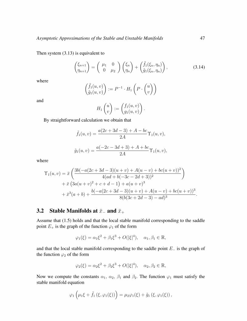
Figure 4.3: The graph of the function U1+(x, y) = 0 (red curve) and U1

−(x, y) = 0 (bluecurve) for a = 1.0, b = 1.0, c = 0.3 and d = 0.2 with the basins of attraction generatedby Dynamica 3.

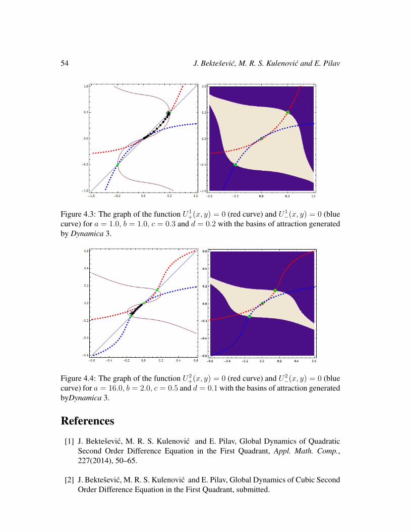
Figure 4.4: The graph of the function U2+(x, y) = 0 (red curve) and U2

−(x, y) = 0 (bluecurve) for a = 16.0, b = 2.0, c = 0.5 and d = 0.1 with the basins of attraction generatedbyDynamica 3.

References

[1] J. Bektesevic, M. R. S. Kulenovic and E. Pilav, Global Dynamics of QuadraticSecond Order Difference Equation in the First Quadrant, Appl. Math. Comp.,227(2014), 50–65.

[2] J. Bektesevic, M. R. S. Kulenovic and E. Pilav, Global Dynamics of Cubic SecondOrder Difference Equation in the First Quadrant, submitted.


[3] A. Brett and M. R. S. Kulenovic, Basins of attraction of equilibrium points ofmonotone difference equations. Sarajevo J. Math. 5(18) (2009), 211–233.

[4] S. Elaydi, Discrete chaos. With applications in science and engineering. Secondedition. With a foreword by Robert M. May., Chapman & Hall/CRC, Boca Raton,FL, 2008.

[5] M. Guzowska, R. Luis and S. Elaydi, Bifurcation and invariant manifolds of thelogistic competition model, J. Difference Equ. Appl., 2011, 17:12, 1851–1872.

[6] J. K. Hale and H. Kocak, Dynamics and bifurcations. Texts in Applied Mathemat-ics, 3. Springer-Verlag, New York, 1991.

[7] M. R. S. Kulenovic and O. Merino, Discrete Dynamical Systems and Differ-ence Equations with Mathematica, Chapman and Hall/CRC, Boca Raton, London,2002.

[8] M. R. S. Kulenovic and O. Merino, Competitive-Exclusion versus Competitive-Coexistence for Systems in the Plane, Discrete Contin. Dyn. Syst. Ser. B 6(2006),1141-1156.

[9] M. R. S. Kulenovic and O. Merino, Global Bifurcation for Competitive Systemsin the Plane, Discrete Contin. Dyn. Syst. B 12(2009), 133-149.

[10] M. R. S. Kulenovic and O. Merino, Invariant manifolds for competitive discretesystems in the plane. Internat. J. Bifur. Chaos Appl. Sci. Engrg. 20 (2010), no. 8,2471–2486.

[11] H. A. Lauwerier, Two-dimensional iterative maps. Chaos, 5895, Nonlinear Sci.Theory Appl., Manchester Univ. Press, Manchester, 1986.

[12] C. Robinson, Stability, Symbolic Dynamics, and Chaos, CRC Press, Boca Raton,1995.

[13] H. L. Smith, Periodic competitive differential equations and the discrete dynamicsof competitive maps, J. Differential Equations 64 (1986), 165-194.

[14] H. L. Smith, Planar Competitive and Cooperative Difference Equations,J. Differ.Equ. Appl. 3(1998), 335-357.

[15] S. Wiggins, Introduction to applied nonlinear dynamical systems and chaos. Sec-ond edition. Texts in Applied Mathematics, 2. Springer-Verlag, New York, 2003.


A Values of Coefficients Υ3, Υ4, Υ5, Γ3, Γ4 and Γ5

Υ4 =2A(ad− 3bc− 2bd+ 3b)3(8a3c3 + 36a3c2d− 36a3c2 + 54a3cd2 − 108a3cd+ 46a3c+ 27a3

d3 − 81a3d2 + 69a3d− 15a3 + 12a2Ac2 + 36a2Acd− 36a2Ac+ 27a2Ad2 − 54a2Ad+ 31a2

A− 12a2bc3 −36a2bc2d+ 36a2bc2 − 27a2bcd2 + 54a2bcd− 39a2bc− 24a2bd+ 24a2b+ 6a

A2c+ 9aA2d− 9aA2 −12aAbc2 − 18aAbcd+ 18aAbc+ 8aAb+ 6ab2c3 + 9ab2c2d− 9ab2c2

− 12ab2d+ 12ab2 +A3 − 3A2bc +3Ab2c2 + 4Ab2 − b3c3 + 4b3c)

Γ4 =2A(ad+ b(−3c− 2d+ 3))3(a3(−(2c+ 3d− 5))(2c+ 3d− 3)(2c+ 3d− 1)

+a2(A(12c2 + 36c(d− 1) + 27(d− 2)d+ 31

)+ 3b

(c(4c2 + 12c(d− 1)

+9(d− 2)d+ 13) + 8(d− 1)))− a(A2(6c+ 9d− 9)

+2Ab(3c(2c+ 3d− 3)− 4) + 3b2(c2(2c+ 3d− 3)− 4d+ 4

))+A3 + 3A2bc

+Ab2(3c2 + 4

)+ b3c

(c2 − 4

))Υ3 =(a+ b)3

(8d3(2c+ 3d− 3)a5 +

(b(16c4 + 96(d− 1)c3 + 72

(d2 − 6d+ 3

)c2 −

8(13d3 + 36d2 − 81d+ 27

)c− 9

(7d4 − 4d3 − 30d2 + 36d− 9

))− 8Ad3

)a4

−4b(A(8c3 + 36(d− 1)c2 + 18

(2d2 − 6d+ 3

)c+ 3

(5d3 − 21d2 + 27d− 9

))+(8c4 − 36(2d+ 1)c3 − 54

(5d2 − 5d− 1

)c2 − 3

(83d3 − 207d2 + 117d+ 9

)c− 18(3− 2d)2(d− 1)d

))a3 − 2b

((204c4 + 36(23d− 26)c3 + 27

(39d2 − 98d+ 59

)c2

+4(3− 2d)2(34d− 33)c+ 12(d− 1)(2d− 3)3)b2 − 6A

(4c3 − 6(d+ 2)

c2 +(−15d2 + 18d+ 9

)c− 2(3− 2d)2d

)b− 3A2(2c+ 3d− 3)2

)a2 + 4b ((−2c− 3d+ 3)

A3 − 3bc(2c+ 3d− 3)A2 + b2(48c3 + 9(11d− 17)c2 + 18(3− 2d)2c+ 2(2d− 3)3

)A

+b3c(52c3 + 3(35d− 53)c2 + 18(3− 2d)2c+ 2(2d− 3)3

))a+ b(A+ bc)4

)− 6(a+ b)3/2

√−c− d+ 1(b(−3c− 2d+ 3) + ad)

(4d2

(4c2 + 4(3d− 4)c

+3(3d2 − 8d+ 5

))a5 +

(8A(2c+ 3d− 2)d2 + b

(16c4 − 112c3 − 8

(19d2 + 3d− 36

)c2

−4(54d3 − 95d2 − 30d+ 81

)c− 9

(7d4 − 22d3 + 16d2 + 14d− 15

)))a4

+2((

56c4 + 4(72d− 89)c3 + 6(80d2 − 204d+ 135

)c2

+3(102d3 − 403d2 + 564d− 267

)c+ 9

(8d4 − 43d3 + 91d2 − 89d+ 33

))b2

+A(−48d3 + 117d2 − 66d+ c2(4− 48d)− 12c

(9d2 − 9d+ 1

)+ 9)b+ 2A2d2

)a3

−2b((

4c2 + 2(12d− 7)c+ 17d2 − 33d+ 12)A2 − 3b

(24c3 + (76d− 72)c2

+2(32d2 − 75d+ 35

)c+ 16d3 − 61d2 + 70d− 21

)A+ b2

(60c4 + 6(30d− 31)c3

+(157d2 − 261d+ 108

)c2 +

(48d3 − 43d2 − 126d+ 117

)c+ 12(3− 2d)2(d− 1)

))a2 + 2b

(−A3 + b

(22c2 + (30d− 41)c+ 8d2 − 21d+ 15

)A2

+b2(−36c3 + (105− 48d)c2 − 2

(8d2 − 45d+ 51

)c

+4(3− 2d)2)A+ b3c

(14c3 + (18d+ 1)c2 +

(8d2 + 15d− 45

)c+ 4(3− 2d)2

))a

+b(A+ bc)2(A2 − 2b(c+ 1)A+ b2c(c+ 2)

))α1


Υ5 =(8d3(2c+ 3d− 3)a5 +

(b(16c4 + 96(d− 1)c3 + 72

(d2 − 6d+ 3

)c2

−8(13d3 + 36d2 − 81d+ 27

)c− 9

(7d4 − 4d3 − 30d2 + 36d− 9

))− 8Ad3

)a4

−4b(A(8c3 + 36(d− 1)c2 + 18

(2d2 − 6d+ 3

)c+ 3

(5d3 − 21d2 + 27d− 9

))+b(8c4 − 36(2d+ 1)c3 − 54

(5d2 − 5d− 1

)c2 − 3

(83d3 − 207d2 + 117d+ 9

)c

−18(3− 2d)2(d− 1)d))a3 − 2b

((204c4 + 36(23d− 26)c3 + 27

(39d2 − 98d+ 59

)c2

+4(3− 2d)2(34d− 33)c+ 12(d− 1)(2d− 3)3)b2 − 6A

(4c3 − 6(d+ 2)c2 +

(−15d2 + 18d

+9) c− 2(3− 2d)2d)b− 3A2(2c+ 3d− 3)2

)a2

+4b((−2c− 3d+ 3)A3 − 3bc(2c+ 3d− 3)A2

+b2(48c3 + 9(11d− 17)c2 + 18(3− 2d)2c+ 2(2d− 3)3

)A

+b3c(52c3 + 3(35d− 53)c2 + 18(3− 2d)2c

+2(2d− 3)3))a+ b(A+ bc)4

)(a+ b)3 + 6

√−c− d+ 1(b(−3c− 2d+ 3) + ad)(

4d2(4c2 + 4(3d− 4)c+ 3

(3d2 − 8d+ 5

))a5 +

(8A(2c+ 3d− 2)d2 + b

(16c4 − 112c3

−8(19d2 + 3d− 36

)c2 − 4

(54d3 − 95d2 − 30d+ 81

)c

−9(7d4 − 22d3 + 16d2 + 14d− 15

)))a4 + 2

((56c4 + 4(72d− 89)c3

+6(80d2 − 204d+ 135

)c2 + 3

(102d3 − 403d2 + 564d− 267

)c

+9(8d4 − 43d3 + 91d2 − 89d+ 33

))b2

+A(−48d3 + 117d2 − 66d+ c2(4− 48d)− 12c

(9d2 − 9d+ 1

)+ 9)b+ 2A2d2

)a3

−2b((

4c2 + 2(12d− 7)c+ 17d2 − 33d+ 12)A2

−3b(24c3 + (76d− 72)c2 + 2

(32d2 − 75d+ 35

)c+ 16d3 − 61d2 + 70d− 21

)A+ b2

(60c4 + 6(30d− 31)c3 +

(157d2 − 261d+ 108

)c2

+(48d3 − 43d2 − 126d+ 117

)c+ 12(3− 2d)2(d− 1)

))a2

+2b(−A3 + b

(22c2 + (30d− 41)c+ 8d2 − 21d+ 15

)A2 + b2

(−36c3 + (105− 48d)c2

−2(8d2 − 45d+ 51

)c+ 4(3− 2d)2

)A+ b3c

(14c3 + (18d+ 1)c2 +

(8d2 + 15d− 45

)c

+4(3− 2d)2))a+ b(A+ bc)2

(A2 − 2b(c+ 1)A+ b2c(c+ 2)

))α2(a+ b)3/2

Γ3 =2(a+ b)3(8d3(2c+ 3d− 3)a5 +

(8Ad3 + b

(16c4 + 96(d− 1)c3 + 72

(d2 − 6d+ 3

)c2 − 8

(13d3 + 36d2 − 81d+ 27

)c− 9

(7d4 − 4d3 − 30d2 + 36d− 9

)))a4

+4b(A(8c3 + 36(d− 1)c2 + 18

(2d2 − 6d+ 3

)c

+3(5d3 − 21d2 + 27d− 9

))+ b

(−8c4 + 36(2d+ 1)c3 + 54

(5d2 − 5d− 1

)c2

+3(83d3 − 207d2 + 117d+ 9

)c+ 18(3− 2d)2(d− 1)d

))a3

+2b(−(204c4 + 36(23d− 26)

c3 + 27(39d2 − 98d+ 59

)c2 + 4(3− 2d)2(34d− 33)c+ 12(d− 1)(2d− 3)3

)b2

−6A(4c3 − 6(d+ 2)c2 +

(−15d2 + 18d+ 9

)c− 2(3− 2d)2d

)b+ 3A2(2c+ 3d− 3)2

)a2

+4b((2c+ 3d− 3)A3 − 3bc(2c+ 3d− 3)A2

−b2(48c3 + 9(11d− 17)c2 + 18(3− 2d)2c+ 2(2d− 3)3

)A+ b3c

(52c3 + 3(35d− 53)c2

+18(3− 2d)2c+ 2(2d− 3)3))a+ b(A− bc)4

)− 6γ1(a+ b)3/2

√1− c− d

(b(−3c− 2d+ 3) + ad)(4d2

(4c2 + 4(3d− 4)c+ 3

(3d2 − 8d+ 5

))a5 +

(b(16c4 − 112c3

−8(19d2 + 3d− 36

)c2 − 4

(54d3 − 95d2 − 30d+ 81

)c


−9(7d4 − 22d3 + 16d2 + 14d− 15

))− 8Ad2(2c+ 3d− 2)

)a4

+2((

56c4 + 4(72d− 89)c3 + 6(80d2 − 204d+ 135

)c2 + 3

(102d3 − 403d2 + 564d− 267

)c

+9(8d4 − 43d3 + 91d2 − 89d+ 33

))b2 +A

(48d3 − 117d2 + 66d+ c2(48d− 4)

+12c(9d2 − 9d+ 1

)− 9)b+ 2A2d2

)a3 − 2b

((4c2 + 2(12d− 7)c+ 17d2 − 33d+ 12

)A2

+3b(24c3 + (76d− 72)c2 + 2

(32d2 − 75d+ 35

)c+ 16d3 − 61d2 + 70d− 21

)A

+b2(60c4 + 6(30d− 31)c3 +

(157d2 − 261d+ 108

)c2

+(48d3 − 43d2 − 126d+ 117

)c+ 12(3− 2d)2(d− 1)

))a2

+2b(A3 + b

(22c2 + (30d− 41)c+ 8d2 − 21d+ 15

)A2 + b2

(36c3 + 3(16d− 35)c2

+2(8d2 − 45d+ 51

)c− 4(3− 2d)2

)A

+b3c(14c3 + (18d+ 1)c2 +

(8d2 + 15d− 45

)c

+4(3− 2d)2))a+ b(A− bc)2

(A2 + 2b(c+ 1)A+ b2c(c+ 2)

)).

Γ5 =(8d3(2c+ 3d− 3)a5 +

(8Ad3 + b

(16c4 + 96(d− 1)c3 + 72

(d2 − 6d+ 3

)c2

−8(13d3 + 36d2 − 81d+ 27

)c− 9

(7d4 − 4d3 − 30d2 + 36d− 9

)))a4

+4b(A(8c3 + 36(d− 1)c2 + 18

(2d2 − 6d+ 3

)c+ 3

(5d3 − 21d2 + 27d− 9

))+b(−8c4 + 36(2d+ 1)c3 + 54

(5d2 − 5d− 1

)c2

+3(83d3 − 207d2 + 117d+ 9

)c+ 18(3− 2d)2(d− 1)d

))a3

+2b(−(204c4 + 36(23d− 26)c3 + 27

(39d2 − 98d+ 59

)c2

+4(3− 2d)2(34d− 33)c+ 12(d− 1)(2d− 3)3)b2 − 6A

(4c3 − 6(d+ 2)c2

+(−15d2 + 18d+ 9

)c− 2(3− 2d)2d

)b+ 3A2(2c+ 3d− 3)2

)a2 + 4b

((2c+ 3d− 3)A3

−3bc(2c+ 3d− 3)A2 − b2(48c3 + 9(11d− 17)c2 + 18(3− 2d)2c+ 2(2d− 3)3

)A

+b3c(52c3 + 3(35d− 53)c2 + 18(3− 2d)2c+ 2(2d− 3)3

))a+ b(A− bc)4

)(a+ b)3

+ 6γ2√−c− d+ 1(b(−3c− 2d+ 3) + ad)

(4d2

(4c2 + 4(3d− 4)c+ 3

(3d2 − 8d+ 5

))a5

+(b(16c4 − 112c3 − 8

(19d2 + 3d− 36

)c2

−4(54d3 − 95d2 − 30d+ 81

)c− 9

(7d4 − 22d3 + 16d2 + 14d− 15

))−8Ad2(2c+ 3d− 2)

)a4 + 2

((56c4 + 4(72d− 89)c3 + 6

(80d2 − 204d+ 135

)c2

+3(102d3 − 403d2 + 564d− 267

)c+ 9

(8d4 − 43d3 + 91d2 − 89d+ 33

))b2

+A(48d3 − 117d2 + 66d+ c2(48d− 4) + 12c

(9d2 − 9d+ 1

)− 9)b

+2A2d2)a3 − 2b

((4c2 + 2(12d− 7)c+ 17d2 − 33d+ 12

)A2 + 3b

(24c3 + (76d− 72)c2

+2(32d2 − 75d+ 35

)c+ 16d3 − 61d2 + 70d− 21

)A+ b2

(60c4 + 6(30d− 31)c3

+(157d2 − 261d+ 108

)c2 +

(48d3 − 43d2 − 126d+ 117

)c+ 12(3− 2d)2(d− 1)

))a2

+2b(A3 + b

(22c2 + (30d− 41)c+ 8d2 − 21d+ 15

)A2 + b2

(36c3 + 3(16d− 35)c2

+2(8d2 − 45d+ 51

)c− 4(3− 2d)2

)A+ b3c

(14c3 + (18d+ 1)c2 +

(8d2 + 15d− 45

)c

+4(3− 2d)2))a+ b(A− bc)2

(A2 + 2b(c+ 1)A+ b2c(c+ 2)

))(a+ b)3/2

Documents

Asymptotic Approximations of the Stable and Unstable Manifolds …campus.mst.edu/ijde/contents/v10n1p3.pdf · 2015-05-01 · Asymptotic Approximations of the Stable and Unstable Manifolds