Improving and BoundingAsymptotic Approximations for

Diversity Combiners inCorrelated Generalized Rician

Fadingby

Joshua Schlenker

B.A.Sc., The University of British Columbia, 2010

A THESIS SUBMITTED IN PARTIAL FULFILLMENT OFTHE REQUIREMENTS FOR THE DEGREE OF

MASTER OF APPLIED SCIENCE

in

The Faculty of Graduate Studies

(Electrical & Computer Engineering)

THE UNIVERSITY OF BRITISH COLUMBIA

(Vancouver)

February 2013

c© Joshua Schlenker 2013

Abstract

Although relatively simple exact error rate expression are available for se-

lection combining (SC) and equal gain combining (EGC) with independent

fading channels, results for correlated channels are highly complex, requiring

multiple levels of integration when more than two branches are involved. Not

only does the complexity make numeric computation resource intensive, it

obscures how channel statistics and correlation affect system performance.

Asymptotic analysis has been used to derive simple error expressions valid

in high signal-to-noise ratio (SNR) regimes. However, it is not clear at what

SNR value the asymptotic results are an accurate approximation of the exact

solution. In this thesis, we derive asymptotic results for SC, EGC, and max-

imal ratio combining (MRC) in correlated generalized Rician fading chan-

nels. By assuming generalized Rician fading, our results incorporate Rician,

Rayleigh, and Nakagami-m fading scenarios as special cases. Furthermore,

the asymptotic results for SC are expanded into an exact infinite series. Al-

though this series grows quickly in complexity as more terms are included,

truncation to even two or three terms has much greater accuracy than the

first (asymptotic) term alone. Finally, we derive asymptotically tight lower

ii

and upper bounds on the error rate for EGC. Using these bounds, we are

able to show at what SNR values the asymptotic results are valid.

iii

Table of Contents

Abstract . . . . . . . . . . . . . . . . . . . . . . . . . . . . . . . . . . ii

Table of Contents . . . . . . . . . . . . . . . . . . . . . . . . . . . . iv

List of Tables . . . . . . . . . . . . . . . . . . . . . . . . . . . . . . viii

List of Figures . . . . . . . . . . . . . . . . . . . . . . . . . . . . . . ix

List of Notation . . . . . . . . . . . . . . . . . . . . . . . . . . . . . xii

List of Abbreviations . . . . . . . . . . . . . . . . . . . . . . . . . . xiv

Acknowledgements . . . . . . . . . . . . . . . . . . . . . . . . . . . xvi

1 Introduction . . . . . . . . . . . . . . . . . . . . . . . . . . . . . 1

1.1 Background and Motivation . . . . . . . . . . . . . . . . . . . 1

1.2 Literature Review . . . . . . . . . . . . . . . . . . . . . . . . 2

1.3 Thesis Outline and Contributions . . . . . . . . . . . . . . . . 6

2 Fading and Diversity Combining . . . . . . . . . . . . . . . . 8

2.1 Multipath Fading . . . . . . . . . . . . . . . . . . . . . . . . 8

iv

2.1.1 Rayleigh Distribution . . . . . . . . . . . . . . . . . . 11

2.1.2 Rician Distribution . . . . . . . . . . . . . . . . . . . 13

2.1.3 Nakagami-m Distribution . . . . . . . . . . . . . . . . 15

2.1.4 Generalized Rician Distribution . . . . . . . . . . . . . 16

2.2 Diversity Combining . . . . . . . . . . . . . . . . . . . . . . . 18

2.3 Generalized Correlation Model . . . . . . . . . . . . . . . . . 20

3 Asymptotic Performance Analysis of Combining Methods in

Generalized Rician Fading . . . . . . . . . . . . . . . . . . . . 26

3.1 System Model . . . . . . . . . . . . . . . . . . . . . . . . . . 27

3.2 Asymptotic Analysis . . . . . . . . . . . . . . . . . . . . . . . 27

3.3 First Order Joint Distributions . . . . . . . . . . . . . . . . . 30

3.4 Combiner Asymptotics . . . . . . . . . . . . . . . . . . . . . . 32

3.4.1 SC . . . . . . . . . . . . . . . . . . . . . . . . . . . . . 32

3.4.2 EGC . . . . . . . . . . . . . . . . . . . . . . . . . . . 33

3.4.3 MRC . . . . . . . . . . . . . . . . . . . . . . . . . . . 34

3.5 Discussion and Numerical Results . . . . . . . . . . . . . . . 34

3.5.1 Discussion . . . . . . . . . . . . . . . . . . . . . . . . 34

3.5.2 Numerical Results . . . . . . . . . . . . . . . . . . . . 37

4 Exact Series Form of the BER with SC in Generalized Rician

Fading . . . . . . . . . . . . . . . . . . . . . . . . . . . . . . . . . 41

4.1 Channel Model . . . . . . . . . . . . . . . . . . . . . . . . . . 41

4.2 SNR Distribution . . . . . . . . . . . . . . . . . . . . . . . . 42

v

4.3 BER of Binary Modulations . . . . . . . . . . . . . . . . . . . 46

4.3.1 BER for Binary Coherent Modulations . . . . . . . . . 46

4.3.2 BER for Binary Noncoherent Modulations . . . . . . . 47

4.4 Convergence and Truncation Error . . . . . . . . . . . . . . . 47

4.4.1 Convergence . . . . . . . . . . . . . . . . . . . . . . . 47

4.4.2 Truncation Error . . . . . . . . . . . . . . . . . . . . . 51

4.5 Numerical Results . . . . . . . . . . . . . . . . . . . . . . . . 52

5 Asymptotically Tight Error Bounds for EGC with General-

ized Rician Fading . . . . . . . . . . . . . . . . . . . . . . . . . 58

5.1 Channel Model . . . . . . . . . . . . . . . . . . . . . . . . . . 58

5.2 Bounds on Joint PDF . . . . . . . . . . . . . . . . . . . . . . 59

5.2.1 Lower Bound . . . . . . . . . . . . . . . . . . . . . . . 60

5.2.2 Upper Bound . . . . . . . . . . . . . . . . . . . . . . . 61

5.3 Error Bounds . . . . . . . . . . . . . . . . . . . . . . . . . . . 65

5.4 Numerical Results . . . . . . . . . . . . . . . . . . . . . . . . 68

6 Conclusion . . . . . . . . . . . . . . . . . . . . . . . . . . . . . . 75

6.1 Summary of Results . . . . . . . . . . . . . . . . . . . . . . . 75

6.2 Future Work . . . . . . . . . . . . . . . . . . . . . . . . . . . 76

Bibliography . . . . . . . . . . . . . . . . . . . . . . . . . . . . . . . 77

vi

Appendices

A Derivation of the Correlation Coefficient ρGkGi . . . . . . . . 85

B Derivation of the Integral Identity (4.7) . . . . . . . . . . . . 87

vii

List of Tables

3.1 Parameters p and q for various coherent modulations . . . . . 29

viii

List of Figures

2.1 The probability density function of a Rayleigh RV with differ-

ent values of Ω. . . . . . . . . . . . . . . . . . . . . . . . . . . 12

2.2 The probability density function of a Rician RV with Ω = 1. . 14

2.3 The probability density function of a Nakagami-m RV with

Ω = 1. . . . . . . . . . . . . . . . . . . . . . . . . . . . . . . . 16

3.1 Performance of EGC and SC relative to MRC. . . . . . . . . . 36

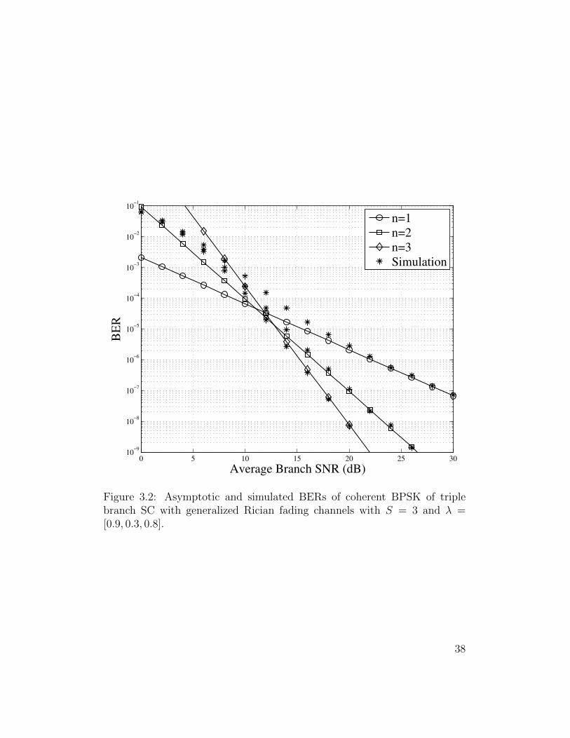
3.2 Asymptotic and simulated BERs of coherent BPSK of triple

branch SC with generalized Rician fading channels with S = 3

and λ = [0.9, 0.3, 0.8]. . . . . . . . . . . . . . . . . . . . . . . . 38

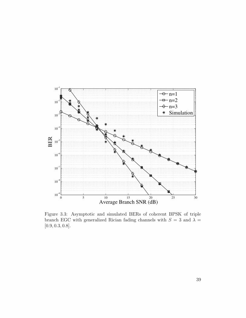
3.3 Asymptotic and simulated BERs of coherent BPSK of triple

branch EGC with generalized Rician fading channels with S =

3 and λ = [0.9, 0.3, 0.8]. . . . . . . . . . . . . . . . . . . . . . . 39

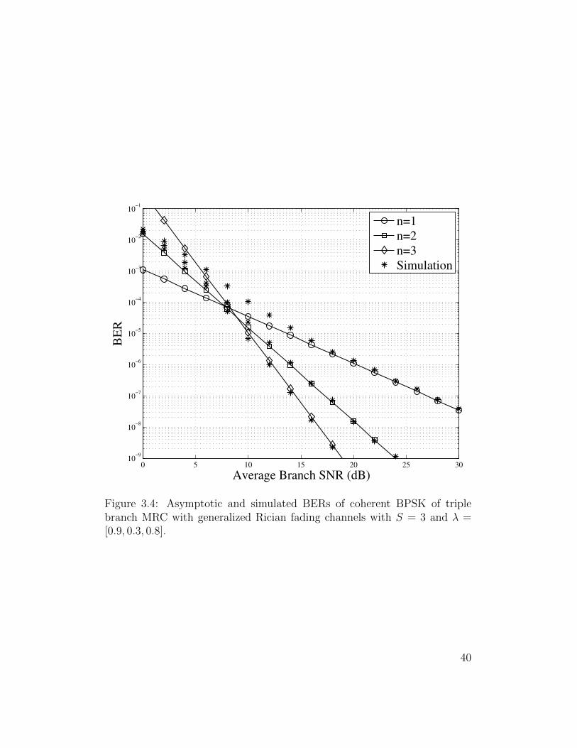
3.4 Asymptotic and simulated BERs of coherent BPSK of triple

branch MRC with generalized Rician fading channels with S =

3 and λ = [0.9, 0.3, 0.8]. . . . . . . . . . . . . . . . . . . . . . . 40

ix

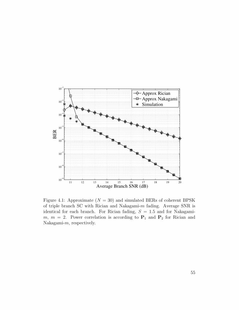
4.1 Approximate (N = 30) and simulated BERs of coherent BPSK

of triple branch SC with Rician and Nakagami-m fading. Av-

erage SNR is identical for each branch. For Rician fading,

S = 1.5 and for Nakagami-m, m = 2. Power correlation is ac-

cording to P1 and P2 for Rician and Nakagami-m, respectively. 55

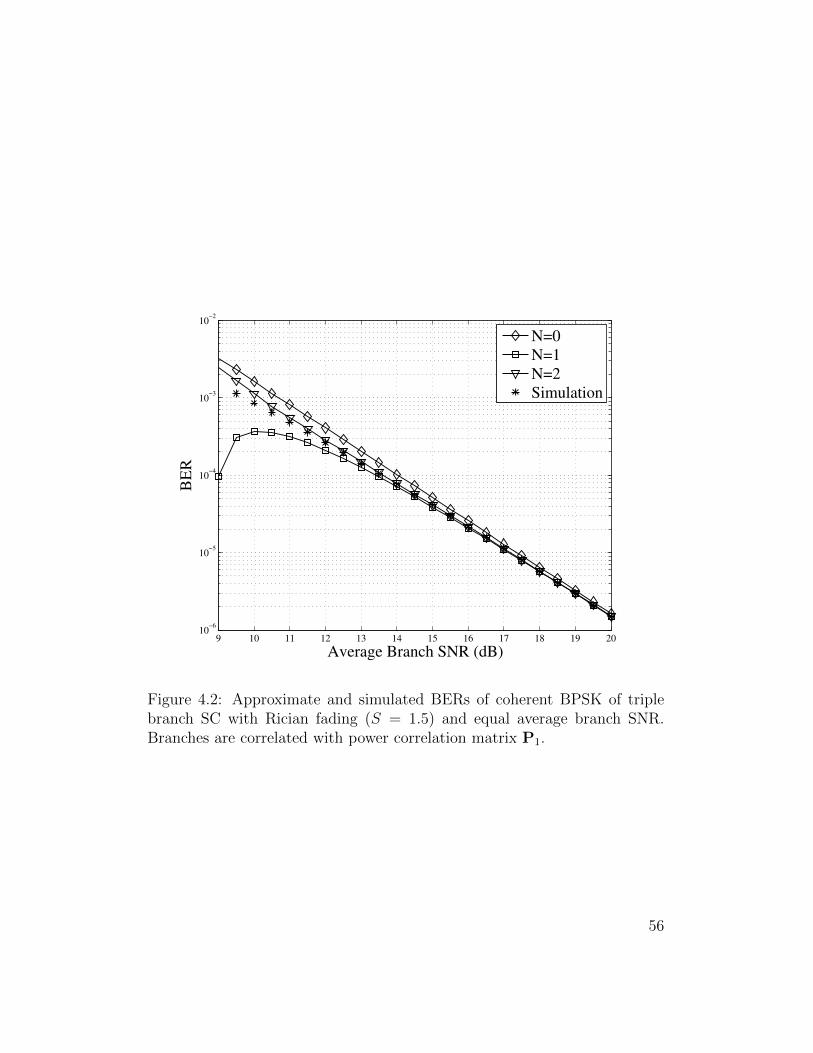
4.2 Approximate and simulated BERs of coherent BPSK of triple

branch SC with Rician fading (S = 1.5) and equal average

branch SNR. Branches are correlated with power correlation

matrix P1. . . . . . . . . . . . . . . . . . . . . . . . . . . . . . 56

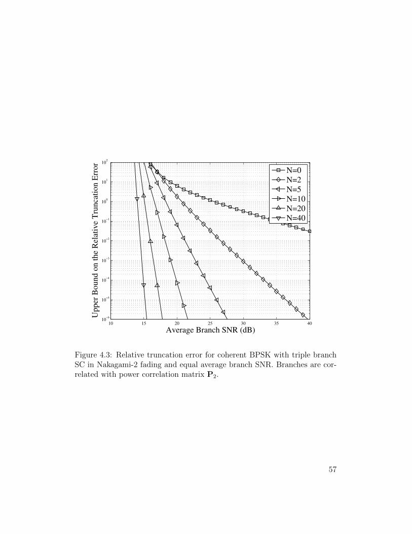
4.3 Relative truncation error for coherent BPSK with triple branch

SC in Nakagami-2 fading and equal average branch SNR. Branches

are correlated with power correlation matrix P2. . . . . . . . . 57

5.1 Upper and lower BER bounds of coherent BPSK over Rayleigh

fading channels with triple branch EGC and equal average

branch SNR. λ = [0.9, 0.8, 0.9] and power correlation matrix P1. 71

5.2 Upper and lower BER bounds of coherent BPSK over Rayleigh

fading channels with triple branch EGC and equal average

branch SNR. λ = [0.5, 0.3, 0.8] and power correlation matrix P2. 72

5.3 Upper and lower BER bounds of coherent BPSK over Nakagami-

1.5 fading channels with triple branch EGC and equal average

branch SNR. λ = [0.2, 0.3, 0.5] and power correlation matrix P3. 73

x

5.4 Upper and lower BER bounds of coherent BPSK over Rician

fading channels (S = 2) with triple branch EGC and equal

average branch SNR. λ = [0.6,−0.4, 0.5] and power correlation

matrix P4. . . . . . . . . . . . . . . . . . . . . . . . . . . . . . 74

xi

List of Notation

| · | Absolute value of a complex number

Iv(·) Modified Bessel function of the first kind with order v, Iv(x) ,∑∞i=0

(x/2)v+2i

i!Γ(v+i+1)

Jv(·) Bessel function of the first kind with order v, Jv(x) ,∑∞i=0

(−1)i(x/2)v+2i

i!Γ(v+i+1)(nk

)Binomial coefficient,

(nk

), n!

k!(n−k)!

ΦX(·) Characteristic function of a random variable X, ΦX(ω) ,

E[ejωX

](·)∗ Conjugate of a complex number

F (·) Dawson’s integral, F (x) , e−x2 ∫ x

0et

2dt

det(·) Determinant of a matrix

E[·] Expectation of a random variable

N ! Factorial of a non-negative integer N , N ! , 1 ·2 · · · (N−1) ·N

and 0! = 1

Γ(·) Euler’s Gamma function, Γ(x) ,∫∞

0tx−1e−tdt

N (µ, σ2) Gaussian distribution with mean µ and variance σ2

xii

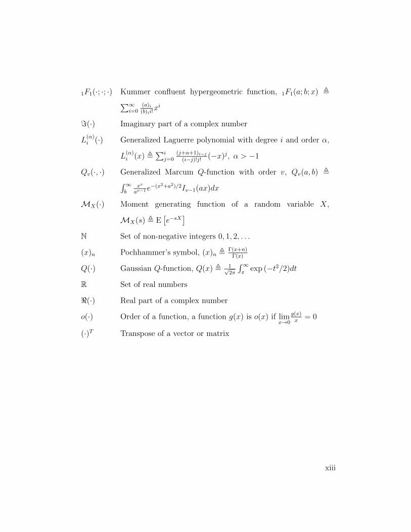
1F1(·; ·; ·) Kummer confluent hypergeometric function, 1F1(a; b;x) ,∑∞i=0

(a)i(b)ii!

xi

=(·) Imaginary part of a complex number

L(α)i (·) Generalized Laguerre polynomial with degree i and order α,

L(α)i (x) ,

∑ij=0

(j+α+1)i−j(i−j)!j! (−x)j, α > −1

Qv(·, ·) Generalized Marcum Q-function with order v, Qv(a, b) ,∫∞b

xv

av−1 e−(x2+a2)/2Iv−1(ax)dx

MX(·) Moment generating function of a random variable X,

MX(s) , E[e−sX

]N Set of non-negative integers 0, 1, 2, . . .

(x)n Pochhammer’s symbol, (x)n , Γ(x+n)Γ(x)

Q(·) Gaussian Q-function, Q(x) , 1√2π

∫∞x

exp (−t2/2)dt

R Set of real numbers

<(·) Real part of a complex number

o(·) Order of a function, a function g(x) is o(x) if limx→0

g(x)x

= 0

(·)T Transpose of a vector or matrix

xiii

List of Abbreviations

AWGN Additive White Gaussian Noise

BCFSK Binary Coherent Frequency Shift Keying

BDPSK Binary Differential Phase Shift Keying

BER Bit Error Rate

BNCFSK Binary Noncoherent Frequency Shift Keying

BPSK Binary Phase Shift Keying

CDF Cumulative Distribution Function

CHF Characteristic Function

EGC Equal Gain Combining

H-S/MRC Hybrid Selection/Maximal Ratio Combining

i.i.d. Independent, Identically Distributed

LOS Line-Of-Sight

MGF Moment Generating Function

M -PAM M -ary Pulse Amplitude Modulation

M -PSK M -ary Phase Shift Keying

M -QAM M -ary Quadrature Amplitude Modulation

MRC Maximal Ratio Combining

xiv

OFDM Orthogonal Frequency Division Multiplexing

PDF Probability Density Function

RF Radio Frequency

RV Random Variable

SC Selection Combining

SER Symbol Error Rate

SNR Signal-to-Noise Ratio

w.r.t. With Respect To

xv

Acknowledgements

I would like to express deep gratitude to my superiors Julian Cheng and

Robert Schober for their hard work and dedication to seeing me through to

the end despite my doubts along the way. Without their insight and expertise

I would scarcely have scratched the surface of what this project became. I

also owe debts of thanks to many colleagues I have encountered in my time at

UBC in Vancouver and the Okanagan, some of whom have become life long

friends. Finally, I would like to thank my parents for their enduring support

and my closest confidant, my girlfriend Kayla, for having the patience to

stick with me through to the end.

Funding for this research was provided by the Natural Sciences and En-

gineering Research Council of Canada (NSERC).

xvi

Chapter 1

Introduction

1.1 Background and Motivation

In recent decades the use of wireless devices has exploded, driven mainly by

the increase in consumer electronics with wireless capabilities, such as cellular

phones, laptops, and GPS units. The mobile nature of these devices and the

multipath propagation of the wireless signal introduces a time variation in

the quality of the channel between transmitter and receiver known as fading.

Without adequate mitigation of this effect, the experience to the end user

would be extremely detrimental, causing dropped phone calls, inability to

load webpages, etc. when a deep fade occurs. One powerful method of com-

bating fading is known as diversity combining. Diversity combining employs

multiple antennas at the receiver, with each branch experiencing different in-

stantaneous signal-to-noise ratios (SNRs) provided the antennas are spaced

sufficiently far apart. The probability that each antenna simultaneously ex-

periences poor channel conditions decreases significantly as more antennas

are added. Although many diversity combining techniques have been studied

in the literature, the three most popular are selection combining (SC), equal

1

gain combining (EGC), and maximal ratio combining (MRC).

Although exact performance analysis of SC, EGC, and MRC has been

widely studied, the results are generally complex, even for independent fad-

ing. For correlated fading with more than two branches, the results are given

in terms of multiple nested infinite series or integrations even for specialized

correlation matrices. This complexity obscures how performance is affected

by fading parameters and the correlation among branches. In response, a

number of research papers have studied the performance when SNR ap-

proaches infinity. This technique is known as asymptotic analysis. The

assumption of high SNR results in a closed-form equation for performance

metrics such as symbol error rate (SER) and outage probability. Although

only strictly valid at infinite SNR, the exact performance can be approx-

imated by the asymptotic results at moderate SNR levels. However, it is

difficult to determine at what SNR value the approximation is valid without

resorting to computationally expensive exact analytical analysis or Monte

Carlo simulations, both of which are susceptible to inaccuracies at low SERs

typical in the high SNR regime.

1.2 Literature Review

The performance analysis of SC, EGC, and MRC for independently faded

channels has been widely studied, and SER expressions are available for a

wide variety of linear modulations which only require a single level of integra-

2

tion regardless of the number of branches. (See [1] and the references therein.)

However, correlation among branches arises when the diversity antennas are

in close proximity, which occurs for devices with space constrained form fac-

tors such as mobile phones. For the general case of L diversity branches and

arbitrary channel correlation, single integral forms and single infinite series

exist for the error rate with MRC at the receiver [2–4]. However, error rate

expressions for EGC and SC are much more complex, typically involving

multi-level integration or infinite series. Expressions with a single integral

or infinite series are only available when the number of branches is limited

to two [5–10]. For L > 2, single integral or infinite series forms for the error

rate are unavailable even for specialized correlation models.

Regarding the SC literature, Karagiannidis et al. obtained a dual infi-

nite series representation of the error rate for a triple branch SC undergoing

Nakagami-m fading with exponential branch correlation [11]. The general

result for arbitrary correlation can be obtained using the joint cumulative

distribution function (CDF) of three Nakagami-m random variables (RVs)

obtained in [12]; however this requires an additional two infinite series. The

joint CDF of L exponentially correlated Nakagami-m RVs was obtained

in [13], consisting of a L − 1 fold infinite series. The results of [13] were

extended to arbitrarily correlated Nakagami-m RVs using a Green’s matrix

approximation of the correlation matrix [14]. Exact results for the most gen-

eral case of arbitrary L and correlation matrix are available for SC but the

complexity of the error rate expressions increases exponentially in L. In [15]

3

the authors took a characteristic function (CHF) approach independent of

the fading distribution; however, the Fourier inversion requires L infinite inte-

grals. A multivariate joint probability density function (PDF) of the general

α− µ distribution consisting of a single infinite sum of generalized Laguerre

polynomials was derived in [16]; however, application to SC performance

analysis requires an L-fold integral of the joint PDF.

The literature for EGC with L > 2 and correlation among the branches is

limited to special correlation models and approximations. In [17], the authors

found the moments at the output of an EGC combiner with Nakagami-m fad-

ing in terms of an L−1 fold infinite summation. The results are approximate

for arbitrarily correlated branches and exact for exponential correlation. The

moment generating function (MGF) can be found from the central moments

via a Taylor series expansion or Pade approximation, from which the error

rate follows with a single integration. A different approach was taken in [18],

where the approximate PDF of a sum of correlated Nakagami-m RVs was

found using moment matching. Using the joint PDF of exponentially corre-

lated Nakagami-m RVs in [13], Sahu and Chaturvedi found the error rates

for coherent BPSK [19] and noncoherent modulations [20]. However, the ex-

pressions are highly complex and involve L−1 fold infinite summation along

with several levels of finite summation.

A novel approach was taken in [21] to find single integral representations

for the CDF of the SNR at the output of a SC combiner with equally cor-

related Nakagami-m, Rayleigh, and Rician fading channels. The correlated

4

RVs are modelled using a linear combination of independent Gaussian RVs.

This allowed the authors to find the error rate using two nested integrals.

Using the same model as [21], Chen and Tellambura found the moments at

the output of an EGC combiner for equally correlated Rayleigh, Rician, and

Nakagami-m fading channels [22]. The authors then presented an approach

for finding the error rate using a single infinite series of the moments. Al-

though the joint PDF was found in single integral form, the moment expres-

sions are L-fold summations of a Lth order Lauricella function. In [23], the

model was generalized for Nakagami-m fading channels and was termed the

‘generalized correlation model’, which was then utilized to derive error rate

and outage probability expressions for hybrid selection/maximal ratio com-

bining (H-S/MRC). Using the generalized correlation model, Beaulieu and

Hemachandra [24] derived single integral forms of the joint PDF and CDF

of Rayleigh, Rician, generalized Rician, Nakagami-m, and Weibull RVs.

The results cited above all require multiple nested levels of integration to

evaluate the exact SER for SC or EGC with correlated fading when L > 2.

Asymptotic analysis allows this complexity to be circumvented by finding

simple SER expressions which are valid only at asymptotically high SNR.

Results for SC, EGC, and MRC are available in the literature. In [25],

Li and Cheng conducted an asymptotic performance analysis for SC with

Nakagami-m fading channels using the generalized correlation model. For

arbitrary correlated Rician channels, the asymptotic results for SC and EGC

can be found in [26]. For arbitrarily correlated Nakagami-m and Rician

5

channels the asymptotic technique was employed to find the SER of MRC

in [27] and [28], respectively.

Although it provides insight into how correlation and fading distribution

parameters affect SER, the major shortcoming of the asymptotic technique

is that it can not predict at what SNR value the asymptotic solutions can

adequately approximate the exact solution. Assessment of the accuracy of

asymptotic solutions for a particular SNR using Monte Carlo simulations

or exact analytical analysis is problematic. Monte Carlo simulation is time

consuming due to the low probability of a symbol error at high SNR, and

the computation of exact analytical solutions requires complex multilevel nu-

meric integration which is also susceptible to error due to the small numerical

values or oscillatory nature of the integrand over the integration region.

1.3 Thesis Outline and Contributions

The remainder of this thesis consists of five chapters. In Chapter 2, we intro-

duce necessary background information relevant to the chapters that follow,

including an overview of fading and diversity combining. Furthermore, the

joint CDF and PDF of generalized Rician RVs correlated according to the

generalized correlation model are derived. In Chapter 3, we find the asymp-

totic error rate expressions for SC, EGC, MRC. In Chapter 4, an infinite

series expansion of the bit error rate (BER) of SC is derived along with the

truncation error when the series is terminated at a finite number of terms.

6

The termination of the series to the first term is the asymptotic error rate.

In Chapter 5, we develop asymptotically tight error bounds for EGC. The

bounds are in the form of a single integration, comparable to the complexity

of computing the exact error rate if the branches were independent. Chap-

ters 3-5 assume generalized Rician fading with generalized correlation among

branches. The results of Chapter 4 and Chapter 5 can be utilized to show at

what SNR the asymptotic error rate is guaranteed to be within a specified

tolerance of the exact error rate. In Chapter 6, we conclude this thesis and

suggest possibilities for related future work.

7

Chapter 2

Fading and Diversity

Combining

In this chapter, we present an overview of the challenges that fading places

on reliable wireless communications and several statistical distributions com-

monly used to model the fading channel. We then introduce several diver-

sity combining techniques which are used to reduce the deleterious effects

of multipath fading when the transmitted signal is sent over multiple fad-

ing channels. In general, the multiple fading channels are correlated, and

we introduce a method to construct generalized Rician RVs for a special

correlation model known as the generalized correlation model.

2.1 Multipath Fading

When a radio frequency (RF) signal is propagated from a transmitter to

receiver wirelessly it typically takes multiple paths due to scattering and

reflections caused by objects in the surrounding environment include build-

ings, roads and cars in an urban environment, and trees and hills in a more

8

rural area. The number of propagation paths can be large, especially in

an urban setting. Each path experiences a different attenuation and phase

delay. When the signals recombine at the receiver, their constructive and

destructive addition results in a phenomenon known as small-scale fading.

Small-scale fading, as opposed to large-scale fading which is the result of

large objects such as buildings or hills located between transmitter and re-

ceiver, is highly location specific. Even motion on the order of centimeters

can cause large fluctuations in the signal strength at the receiver due to the

high carrier frequencies in typical wireless communication systems. For ex-

ample, if a mobile phone operates with a carries frequency of 2 GHz, with a

corresponding wavelength of approximately 15 cm, even a small movement

by the mobile user could cause the signal strength to transition from rel-

atively strong to weak. In this thesis, we only consider small-scale fading,

which we will simply refer to as fading. This is a common assumption in the

literature.

A deterministic treatment of the wireless channel is not practical due

to large number of propagation paths and random movements of the users

and surrounding objects. Thus, fading is typically modelled as a random

process. The fading channel is characterized by its coherence time and band-

width. The coherence time, roughly speaking, is the length of time the fading

coefficient can be considered as approximately constant. Signals with a sym-

bol duration smaller than the coherence time will experience slow fading,

where the channel conditions are constant throughout the symbol duration.

9

A signal with a symbol duration longer than the channel coherence time

will experience fast fading, where the fading coefficient changes during sym-

bol transmission. Coherence bandwidth is a frequency-domain description

of fading channels. A transmitted symbol with a bandwidth larger than

the channel coherence bandwidth will experience frequency selective fading

whereas when the opposite is true, each frequency in the transmitted symbol

will experience approximately identical fading resulting in frequency nonse-

lective or flat fading. In slow, frequency nonselective fading, the channel can

be described by the complex gain hejθ for the duration of the transmitted

symbol, where h and θ are the random fading envelope and phase respec-

tively. We will assume slow, frequency nonselective fading in this thesis. In

situations where the channel is frequency selective, it can be divided into

multiple frequency nonselective channels using orthogonal frequency division

multiplexing (OFDM) [30]. Though there exists a large number of statisti-

cal models for h, each tailored to specific fading environments, three widely

adopted fading models are Rayleigh, Rician, and Nakagami-m.

The effect of fading on receiver performance is significant. In a constant

channel gain, i.e. no fading, in the high SNR regime, a binary phase shift

keying (BPSK) modulated signal has the BER

Pe ≈1

2√πγe−γ (2.1)

where γ is the average SNR at the receiver. The identical receiver in a

10

Rayleigh fading channel experiences a BER at large SNR of [31]

Pe ≈1

4γ. (2.2)

In effect, the presence of fading has reduced the BER from being exponential

in γ to only linear. At typical SNRs, fading increases the error rate by several

orders of magnitude. For example, at 10 dB a constant gain channel would

experience a BER of approximately 5×10−5, while a Rayleigh faded channel

would experience a BER of roughly 2×10−2. As this is also only the average

error rate, the instantaneous error rate can even be worse.

2.1.1 Rayleigh Distribution

When the complex channel gain is modelled as a zero mean Gaussian RV

with independent, identically distributed (i.i.d.) real and imaginary parts,

the fading envelop follows the Rayleigh distribution. This model best fits

environments in which the transmitted signal is scattered and reflected mul-

tiple times before reaching the receiver without a line-of-sight (LOS) path.

By a central limit theorem, the sum of all signal paths at the receiver will

have a zero-mean Gaussian distribution. The Rayleigh RV X has a PDF of

fX(x) =2x

σ2e−

x2

σ2 (2.3)

11

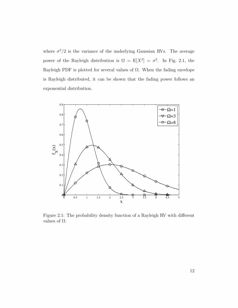
where σ2/2 is the variance of the underlying Gaussian RVs. The average

power of the Rayleigh distribution is Ω = E[X2] = σ2. In Fig. 2.1, the

Rayleigh PDF is plotted for several values of Ω. When the fading envelope

is Rayleigh distributed, it can be shown that the fading power follows an

exponential distribution.

0 0.5 1 1.5 2 2.5 3 3.5 4 4.5 50

0.1

0.2

0.3

0.4

0.5

0.6

0.7

0.8

0.9

f X(x

)

x

Ω=1

Ω=3

Ω=8

Figure 2.1: The probability density function of a Rayleigh RV with differentvalues of Ω.

12

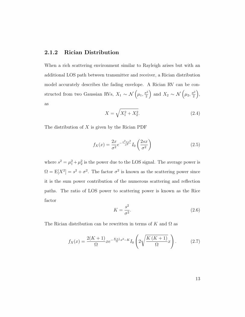
2.1.2 Rician Distribution

When a rich scattering environment similar to Rayleigh arises but with an

additional LOS path between transmitter and receiver, a Rician distribution

model accurately describes the fading envelope. A Rician RV can be con-

structed from two Gaussian RVs, X1 ∼ N(µ1,

σ2

2

)and X2 ∼ N

(µ2,

σ2

2

),

as

X =√X2

1 +X22 . (2.4)

The distribution of X is given by the Rician PDF

fX(x) =2x

σ2e−

x2+s2

σ2 I0

(2sx

σ2

)(2.5)

where s2 = µ21 +µ2

2 is the power due to the LOS signal. The average power is

Ω = E[X2] = s2 + σ2. The factor σ2 is known as the scattering power since

it is the sum power contribution of the numerous scattering and reflection

paths. The ratio of LOS power to scattering power is known as the Rice

factor

K =s2

σ2. (2.6)

The Rician distribution can be rewritten in terms of K and Ω as

fX(x) =2(K + 1)

Ωxe−

K+1Ω

x2−KI0

(2

√K (K + 1)

Ωx

). (2.7)

13

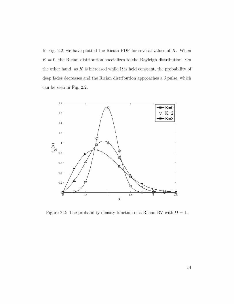
In Fig. 2.2, we have plotted the Rician PDF for several values of K. When

K = 0, the Rician distribution specializes to the Rayleigh distribution. On

the other hand, as K is increased while Ω is held constant, the probability of

deep fades decreases and the Rician distribution approaches a δ pulse, which

can be seen in Fig. 2.2.

0 0.5 1 1.5 2 2.50

0.2

0.4

0.6

0.8

1

1.2

1.4

1.6

1.8

f X(x

)

x

K=0

K=2

K=8

Figure 2.2: The probability density function of a Rician RV with Ω = 1.

14

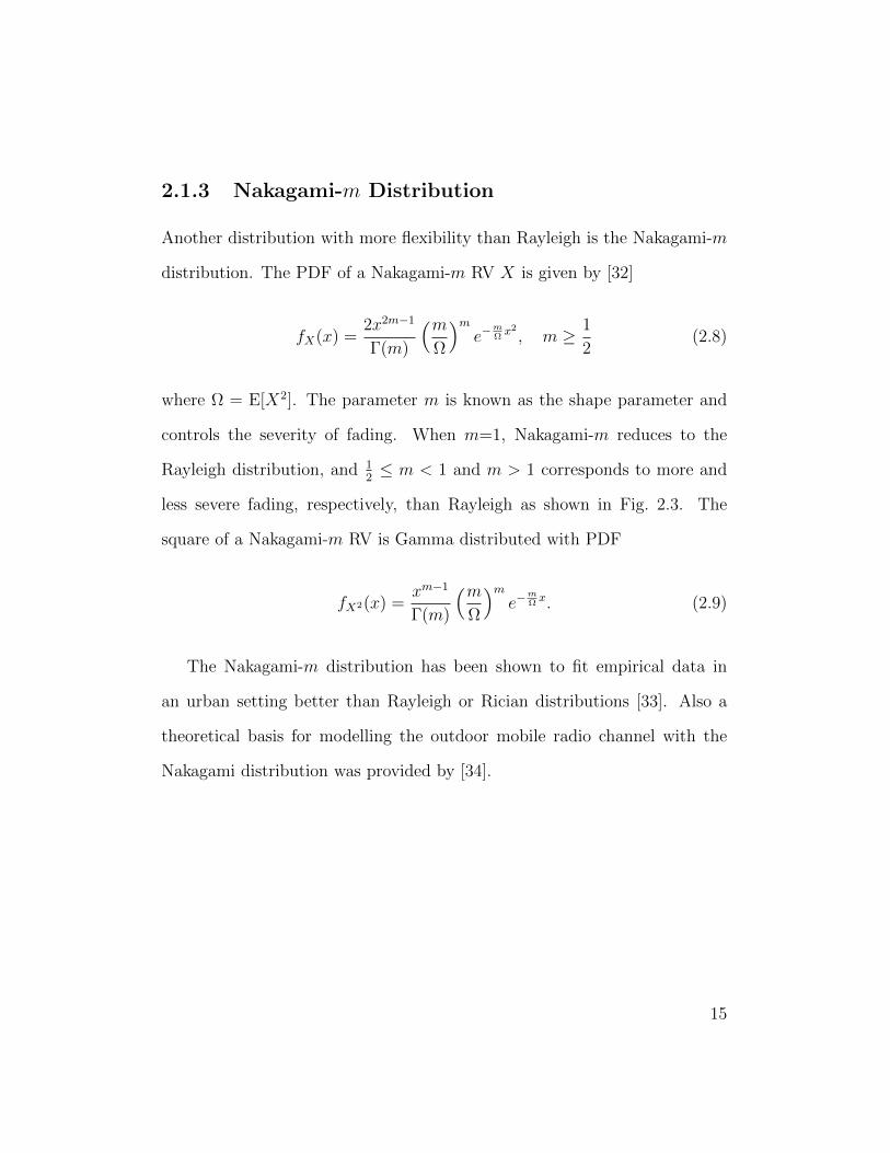
2.1.3 Nakagami-m Distribution

Another distribution with more flexibility than Rayleigh is the Nakagami-m

distribution. The PDF of a Nakagami-m RV X is given by [32]

fX(x) =2x2m−1

Γ(m)

(mΩ

)me−

mΩx2

, m ≥ 1

2(2.8)

where Ω = E[X2]. The parameter m is known as the shape parameter and

controls the severity of fading. When m=1, Nakagami-m reduces to the

Rayleigh distribution, and 12≤ m < 1 and m > 1 corresponds to more and

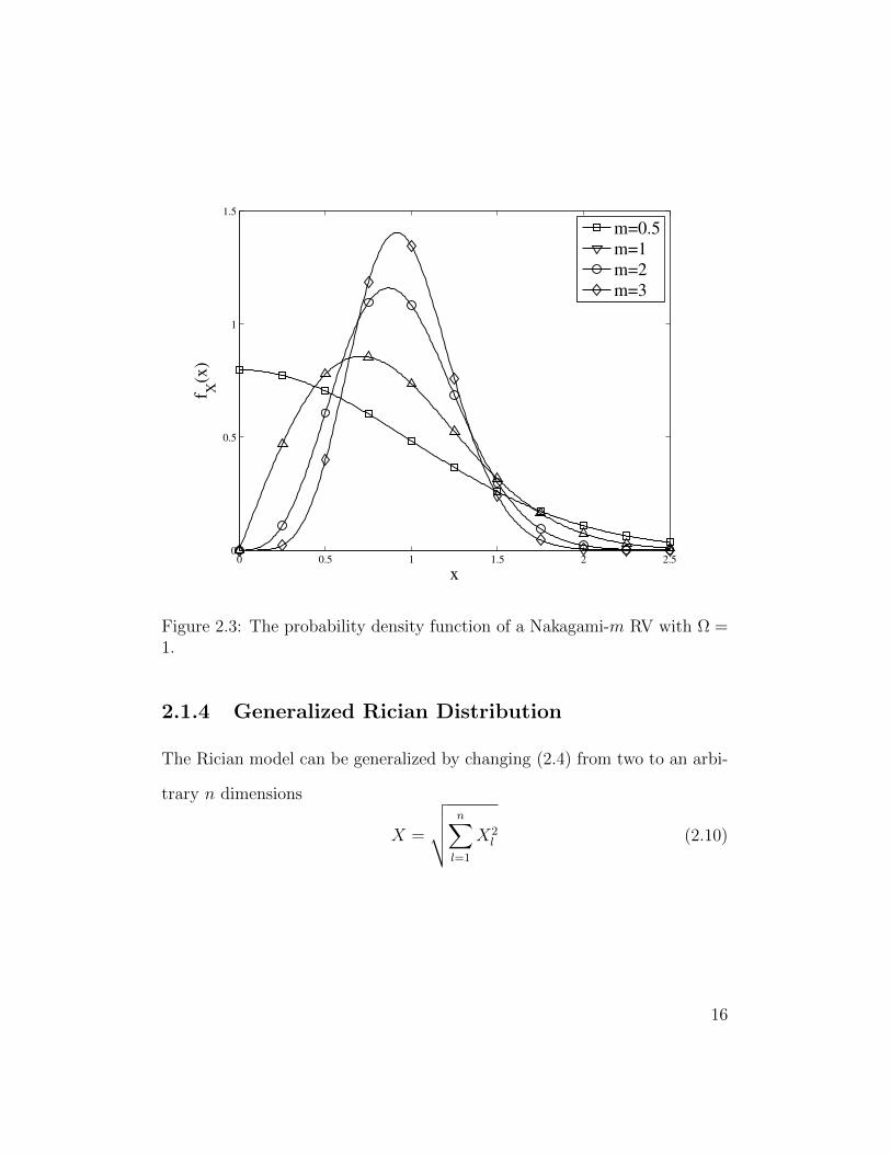
less severe fading, respectively, than Rayleigh as shown in Fig. 2.3. The

square of a Nakagami-m RV is Gamma distributed with PDF

fX2(x) =xm−1

Γ(m)

(mΩ

)me−

mΩx. (2.9)

The Nakagami-m distribution has been shown to fit empirical data in

an urban setting better than Rayleigh or Rician distributions [33]. Also a

theoretical basis for modelling the outdoor mobile radio channel with the

Nakagami distribution was provided by [34].

15

0 0.5 1 1.5 2 2.50

0.5

1

1.5f X

(x)

x

m=0.5

m=1

m=2

m=3

Figure 2.3: The probability density function of a Nakagami-m RV with Ω =1.

2.1.4 Generalized Rician Distribution

The Rician model can be generalized by changing (2.4) from two to an arbi-

trary n dimensions

X =

√√√√ n∑l=1

X2l (2.10)

16

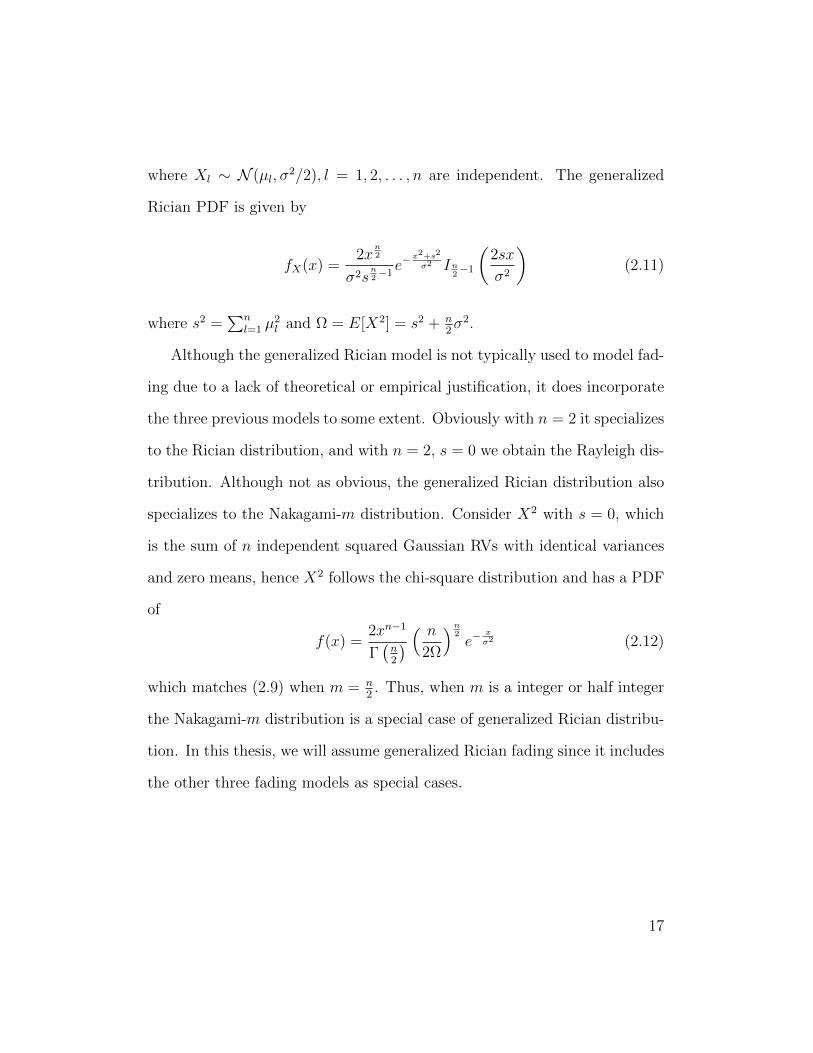
where Xl ∼ N (µl, σ2/2), l = 1, 2, . . . , n are independent. The generalized

Rician PDF is given by

fX(x) =2x

n2

σ2sn2−1e−

x2+s2

σ2 In2−1

(2sx

σ2

)(2.11)

where s2 =∑n

l=1 µ2l and Ω = E[X2] = s2 + n

2σ2.

Although the generalized Rician model is not typically used to model fad-

ing due to a lack of theoretical or empirical justification, it does incorporate

the three previous models to some extent. Obviously with n = 2 it specializes

to the Rician distribution, and with n = 2, s = 0 we obtain the Rayleigh dis-

tribution. Although not as obvious, the generalized Rician distribution also

specializes to the Nakagami-m distribution. Consider X2 with s = 0, which

is the sum of n independent squared Gaussian RVs with identical variances

and zero means, hence X2 follows the chi-square distribution and has a PDF

of

f(x) =2xn−1

Γ(n2

) ( n

2Ω

)n2e−

xσ2 (2.12)

which matches (2.9) when m = n2. Thus, when m is a integer or half integer

the Nakagami-m distribution is a special case of generalized Rician distribu-

tion. In this thesis, we will assume generalized Rician fading since it includes

the other three fading models as special cases.

17

2.2 Diversity Combining

A common method for mitigating fading is to employ diversity at the receiver.

Multiple copies of the transmitted signal are made available to the receiver,

each experiencing different fading channels. The probability that all fading

channels are in deep fade simultaneously decreases rapidly as diversity is

increased. Receive diversity can be achieved by transmitting the same symbol

over multiple frequencies or time slots. However, this requires additional

bandwidth. To circumvent this problem, the receiver can employ multiple

antennas, each receiving the transmitted signal over different fading channels.

In general, the channels are correlated due to space constraints in small

form factors, such as mobile phones, which requires antennas to be in close

proximity. Branches in a system employing time or frequency diversity will

be correlated if duplicate transmissions occur within the coherence time or

coherence bandwidth respectively.

There are several methods to combine the received signals, each with a

different performance-complexity trade off. Suppose that the receiver has L

branches of diversity available, and the transmitted symbol with energy ES

is subject to a fading channel with complex channel gain hkejθk and additive

white Gaussian noise (AWGN) with power spectral density N0 on the kth

branch. The instantaneous SNR on branch k is then γk = h2kESN0

. A linear

combiner multiplies the signal on the kth branch by a complex weight wk,

then sums the result. The instantaneous SNR at the output of a general

18

linear combiner is then

γc =

∣∣∣∑Lk=1wkhke

jθk

∣∣∣2∑Lk=1 |wk|2

ESN0

. (2.13)

The simplest combining technique would be to only consider the branch

with the largest SNR and perform signal detection on this branch exclu-

sively. This technique is known as SC. For SC, wi = 1 and wk = 0, k =

1, 2, . . . , L, k 6= i where i = arg maxk=1,2,...,L γk. SC has an instantaneous

SNR at the combiner output of

γSC = maxk=1,2,...,L

γk. (2.14)

Beyond its implementation simplicity, SC is also advantageous for noncoher-

ent modulations since it does not require knowledge of the channel phases.

Although all the other branches may have lower SNRs, they still contain

valuable information about the transmitted signal. A more complex combin-

ing technique that utilizes all available branches is known as EGC. EGC uses

the weight wk = e−jθk , phase aligning each branch before summation. This

technique requires phase knowledge for each branch and is suitable only for

coherent modulations. EGC has an instantaneous SNR of

γEGC =

(∑Lk=1

√γk

)2

L. (2.15)

19

Although performance of EGC is better in most cases than SC, this may

not be true in severe fading [35] or exponentially decaying average branch

SNRs [36].

With EGC, we treat each branch identically regardless of the individ-

ual SNRs of each branch. A more sophisticated method is to weigh the

contribution of each branch according to the severity of the fading by recog-

nizing that branches with high SNR are more trustworthy than those with

lower SNR. This combining method is known as MRC, which has the weight

wk = hke−jθk . MRC has an instantaneous SNR at the output of the combiner

of

γMRC =L∑k=1

γk. (2.16)

Applying the Cauchy-Swartz inequality to (2.13), one can prove that MRC

is the optimal linear combining scheme in terms of maximizing the combiner

output SNR. Although MRC is optimal, it requires knowledge of the fading

envelope and phase, thus analysis of the simpler EGC and SC is of practical

interest.

2.3 Generalized Correlation Model

In general, the fading channels of a diversity combiner are correlated, thus we

require the joint statistics of the channel to analyze combiner performance.

In this section, we present the method of Beaulieu and Hemachandra for

obtaining single integral representations of the multivariate joint PDF and

20

CDF of correlated generalized Rician RVs [24]. Consider the following1

Xkl = σk

(√1− λ2

kUkl + λkU0l

), k = 1, 2, . . . , L, l = 1, 2, . . . , n (2.17)

where −1 < λk < 1, Ukl ∼ N (0, 12), k = 1, 2, . . . , L, l = 1, 2, . . . , n, and

U0l ∼ N(ml,

12

), l = 1, 2, . . . , n, Ukl and Uij are independent for k 6= i

or l 6= j. Each Xkl is the sum of independent Gaussian RVs and hence a

Gaussian RV itself with Xkl ∼ N(σkλkml,

σ2k

2

). For a given l, U0l is common

to Xkl for k = 1, 2, . . . , L, it then follows that the Xkl’s are correlated RVs.

Define the correlation coefficient between two RVs X and Y as

ρXY ,E [XY ]− E [X] E [Y ]√

Var[X]Var[Y ](2.18)

where Var[X] is the variance of RV X. The correlation coefficient between

Xkl and Xij is given by

ρXklXij =

1 k = i, l = j

λkλi k 6= i, l = j

0 l 6= j

. (2.19)

1We have removed the imaginary part of [24, Eq. (11)] to match the conventional formof the generalized Rician model given in [31].

21

Since for a given k, the Xkl are a set of independent Gaussian RVs with

identical variance σk and non-zero means, Gk =∑n

l=1 X2kl and Rk =

√Gk,

k = 1, 2, . . . L, are a noncentral χ2 and generalized Rician RV, respectively.

It is shown in Appendix A that the correlation between Gi and Gk is

ρGkGi = ρR2kR

2i

=λ2kλ

2i (n2

+ 2S2)√n2

+ 2λ2kS

2√

n2

+ 2λ2iS

2, k 6= i (2.20)

where S2 =∑n

l=1m2l . For Nakagami-m fading, (2.20) reduces to

ρGkGi = ρR2kR

2i

= λ2kλ

2i , k 6= i. (2.21)

To find the joint PDF of R = [R1, R2, . . . , RL], we remove the dependence

by conditioning Xkl on U0l, which is a Gaussian RV with E[Xkl|U0l] = σkλkU0l

and Ωk = Var[Xkl|U0l] =σ2k(1−λ2

k)

2. It follows then that Gk conditioned on

U0l, l = 1, 2, . . . , n is noncentral χ2 distributed with PDF

fGk|T (gk) =1

2Ω2k

(gk

σ2kλ

2kT

)n−24

e−x+λ2

kσ2kT

2Ω2k In

2−1

(√gkσ2

kλ2kT

Ω2k

)(2.22)

where T =∑n

l=1 U20l, and we have used the fact that conditioning on U0l, l =

1, 2, . . . , n is identical to conditioning on T . T is a noncentral χ2 RV with

PDF

fT (t) =

(t

S2

)n−24

e−(t+S2)In2−1

(2S√t). (2.23)

SinceGk’s conditioned on T are independent, the joint PDF of G = [G1, G2, . . . , GL]

22

conditioned on T is then

fG|T (g1, g2, . . . , gL) =L∏k=1

1

2Ω2k

(gk

σ2kλ

2kT

)n−24

e− gk+λ2

kσ2kT

2Ω2k In

2−1

(√gkσ2

kλ2kT

Ω2k

).

(2.24)

We obtain the joint PDF of G by taking the expectation of (2.24) with

respect to (w.r.t.) the PDF of T

fG(g1, g2, . . . , gL) =

∞∫0

(t

S2

)n−24

e−(t+S2)In2−1

(2S√t)

×L∏k=1

1

2Ω2k

(gk

σ2kλ

2kt

)n−24

exp

(−gk + λ2

kσ2kt

2Ω2k

)In

2−1

(√gkσ2

kλ2kt

Ω2k

)dt. (2.25)

By definition, the joint CDF of G is

FG(g1, g2, . . . , gL)

=

g1∫0

g2∫0

· · ·gL∫

0

fG(x1, x2, . . . , xL)dx1dx2 · · · dxL

=

∞∫0

(t

S2

)n−24

e−(t+S2)In2−1

(2S√t) L∏k=1

[1−Qn

2

(√2λ2

kt

1− λ2k

,

√gk

Ωk

)]dt

(2.26)

where we have used the property Qv(a, 0) = 1. We can now obtain the joint

23

CDF of R from (2.26) as follows

FR(r1,r2, . . . , rL)

=Pr[r1 ≤

√G1, r2 ≤

√G2, rL ≤

√GL

]=FG(r2

1, r22, . . . , r

2L)

=

∞∫0

(t

S2

)n−24

e−(t+S2)In2−1

(2S√t) L∏k=1

[1−Qn

2

(√2λ2

kt

1− λ2k

,rkΩk

)]dt.

(2.27)

Taking the partial differentiation of (2.27) w.r.t. r1, r2, . . . , rL, we obtain the

joint PDF of R as

fR(r1, r2, . . . , rL) =exp (−S2)

Sn2−1

∞∫0

tn−2

4 exp (−t)In2−1(2S

√t)

×L∏k=1

rn2k

(λ2kσ

2kt)

n−24 Ω2

k

exp

−r

2k + λ2

kσ2kt

2Ω2k

In

2−1

(rk√σ2kλ

2kt

Ω2k

)dt. (2.28)

Although [24] justifies the relevance of the generalized correlation model

by pointing out the lack of simple PDF and CDF expressions for commonly

used fading models with L > 2, it does not discuss the limitations of the

model. Let us examine the marginal PDF of Rk, which can be found by

setting ri =∞ for i = 1, 2, . . . , L, i 6= k in (2.27), then differentiating w.r.t.

24

to rk to obtain

fRk(rk) =2r

n2k

(λkσkS)n2−1σ2

k

exp

(−λ2

kS2 − r2

k

σ2k

)In

2−1

(2λkSrkσk

)(2.29)

where we have also used the integral identity [37, Eq. (3.25.17.1)]. Compar-

ing (2.29) to the generalized Rician PDF (2.11), we see that s2k = λ2

kσ2kS

2 in

the generalized correlation model. Since the parameter S is identical in the

marginal PDF of each Rk, k = 1, 2, . . . , L, si cannot be chosen independently

of sk for i 6= k. For Rician fading, this translates to a dependence among

the Rice factors. Of course, this limitation does not apply to the Rayleigh

and Nakagami-m special cases since sk = 0. The second limitation is that

the power correlation coefficients of R (2.20) cannot be arbitrarily chosen for

L > 3. There are (L2−L)/2 correlation coefficients, but only L number of λ

coefficients. When L > 3, (L2 − L)/2 > L and there are not enough degrees

of freedom available to arbitrarily choose each correlation coefficient. The

generalized correlation model does however include the special case of equal

correlation when λk = λ, k = 1, 2, . . . L. Despite the limitations we have

outlined here, we will adopt the generalized correlation model for this thesis

in the absence of a tractable analytical model for arbitrary correlation.

25

Chapter 3

Asymptotic Performance

Analysis of Combining Methods

in Generalized Rician Fading

In this chapter, we derive the asymptotic error rates of SC, EGC, and MRC

for coherent and noncoherent modulations in correlated generalized Rician

fading channels. Although using our results, asymptotic error rates can be

found for all combinations of signal modulations and combining schemes we

consider, some of combinations are not useful in practice, e.g. asymptotic

error rates of noncoherent modulations with EGC and MRC combiners.

As mentioned in Chapter 1, some results derived here are not original,

as asymptotic error rate expressions for Rician and Nakagami-m fading with

generalized correlation are a special case of those in [26–28]. The case of

Nakagami-m fading with SC is also identical to the results in [25]. How-

ever, the asymptotic SC results are expanded into an exact infinite series in

Chapter 4 with an upper bound on the truncation error. In addition, asymp-

totically tight bounds on the error rate under EGC are derived in Chapter 5.

26

The results of Chapters 4 and 5 can guarantee the minimum SNR at which

the asymptotic error rates given here are within a tolerance of the exact

error rate. The results for MRC are derived here for completeness and for

comparison to SC and EGC.

3.1 System Model

Consider an L-branch diversity combiner where the transmitted signal is im-

paired by slow, frequency nonselective fading and AWGN on each branch.

The instantaneous SNR on the kth branch is γk = R2k, where Rk is a general-

ized Rician RV. We assume correlation among branches fits the generalized

correlation model discussed in Chapter 2, then the average SNR on the kth

branch is γk = E[γk] = σ2k

(n2

+ λ2kS

2), and power correlation between the

kth and ith branch is

ργkγi =λ2kλ

2i (n2

+ 2S2)√n2

+ 2λ2kS

2√

n2

+ 2λ2iS

2, k 6= i. (3.1)

3.2 Asymptotic Analysis

Let us assume a generic receiver where γ is the instantaneous SNR at the

demodulator with average SNR γ = E [γ] and PDF fγ(γ). If the conditional

SER for a constant (non fading) channel is Pe|γ, then the SER for a fading

27

channel is given by

Pe =

∞∫0

Pe|γfγ(γ)dγ. (3.2)

It turns out that when the average SNR approaches infinity, the error prob-

ability is solely determined by the shape of the fγ(γ) at the origin [27]. This

can be intuitively explained as follows. The conditional error rate decreases

exponentially in SNR due to the nature of Gaussian noise, thus even for

moderate γ, Pe is mostly determined by the probability that γ is small since

Pe|γ will be several orders of magnitude greater at γ = 0 than at γ = γ. Let

the first-order approximation of fγ(γ) at the origin be given by

fγ(γ) = aγt + o(γt). (3.3)

Using (3.3) in conjunction with (3.2) we can produce an approximation of

Pe. As γ → ∞, Pe is increasingly dominated by the probability that γ is

near zero, and the approximation approaches the exact solution.

At high SNR, many coherent modulations have a conditional error proba-

bility in the form of pQ(√qγ) including BPSK, M -ary pulse amplitude mod-

ulation (M -PAM), M -ary phase shift keying (M -PSK), and M -ary quadra-

ture amplitude modulation (M -QAM) [31]. The parameters p and q for

these modulations are listed in Table 3.1. The asymptotic SER with con-

ditional error probability pQ(√qγ) and the first-order approximation of the

28

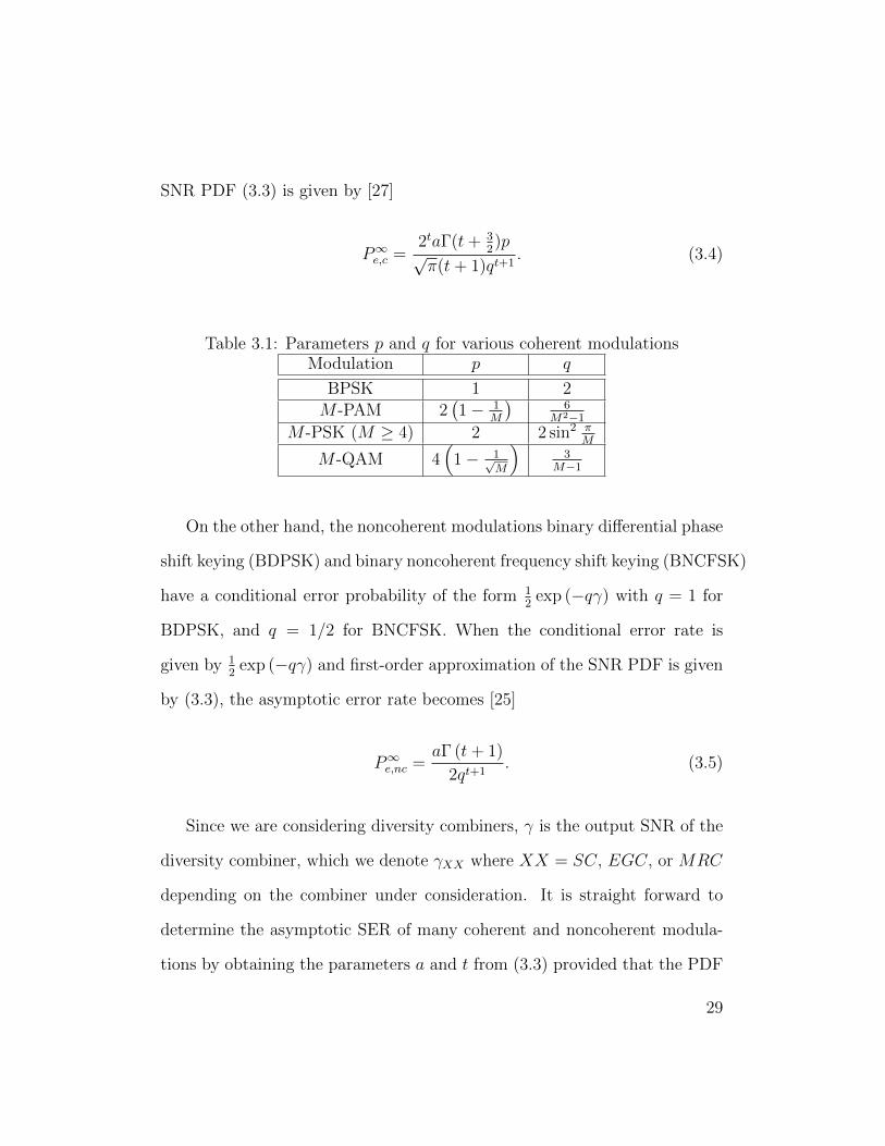
SNR PDF (3.3) is given by [27]

P∞e,c =2taΓ(t+ 3

2)p

√π(t+ 1)qt+1

. (3.4)

Table 3.1: Parameters p and q for various coherent modulationsModulation p q

BPSK 1 2M -PAM 2

(1− 1

M

)6

M2−1

M -PSK (M ≥ 4) 2 2 sin2 πM

M -QAM 4(

1− 1√M

)3

M−1

On the other hand, the noncoherent modulations binary differential phase

shift keying (BDPSK) and binary noncoherent frequency shift keying (BNCFSK)

have a conditional error probability of the form 12

exp (−qγ) with q = 1 for

BDPSK, and q = 1/2 for BNCFSK. When the conditional error rate is

given by 12

exp (−qγ) and first-order approximation of the SNR PDF is given

by (3.3), the asymptotic error rate becomes [25]

P∞e,nc =aΓ (t+ 1)

2qt+1. (3.5)

Since we are considering diversity combiners, γ is the output SNR of the

diversity combiner, which we denote γXX where XX = SC, EGC, or MRC

depending on the combiner under consideration. It is straight forward to

determine the asymptotic SER of many coherent and noncoherent modula-

tions by obtaining the parameters a and t from (3.3) provided that the PDF

29

at the output of the combiner, fγXX (γ), is available. While this approach is

feasible for SC, it is difficult to directly determine the PDF of the sum of

RVs directly, as is the case with MRC and EGC. In these cases, a Laplace

transform approach is often employed. For this approach, we require the

MGF of γ, defined as Mγ(s) = E [e−sγ], to be

Mγ(s) =aΓ(t+ 1)

st+1+ o

(1

st+1

)(3.6)

as s → ∞. Alternatively, we can also find a, and t from the MGF of the

equivalent channel at the output of the combiner, h =√γ. The MGF of h

when s→∞ is

Mh(s) =2aΓ(2t+ 2)

s2t+2+ o

(1

s2t+2

). (3.7)

3.3 First Order Joint Distributions

In order to determine the first-order approximation of γ at the origin we first

find the joint PDF and the joint CDF of R = [R1, R2, . . . , RL] near the origin.

From a Taylor series expansion of the exponential function, limx→0

exp(x) =

1 + o(1) and from the series expansion of the modified Bessel function of the

first kind [39, Eq. (9.6.10)], limx→0

Iv(x) = 1Γ(v+1)

(12x)v

+ o(xv+1). Substituting

these asymptotic expression into the joint PDF of R (2.28) we find

fR(r1, . . . , rL) =2Le−

ΛΛ+1

S2

ΓL(n2

)det

n2 (M)

(∏Lk=1 σ

2k

)n2

L∏k=1

(rn−1k + o(rn−1

k )) (3.8)

30

where Λ =∑L

k=1

λ2k

1−λ2k. In obtaining (3.8), we have used an integral iden-

tity [40, Eq. (6.643.2)] and performed algebraic simplifications using [40, Eq.

(9.220.2)] and [39, Eq. (13.6.12)]. We have also introduced the correlation

matrix M

M =

1 λ1λ2 · · · λ1λL

λ1λ2 1 · · · ...

......

. . . λL−1λL

λ1λL · · · λL−1λL 1

(3.9)

where det(M) =[1 +

∑Lk=1

λ2k

1−λ2k

]∏Lk=1(1 − λ2

k). This result can be found

by expressing M as a rank 1 update matrix and using a matrix determinant

lemma [25]. The off diagonal elements of M are the correlation coefficients

of the underlying Gaussian RVs in R which were given in (2.19). The CDF

of R can be found by integrating (3.8) over r1, r2, . . . , rL, resulting in

FR(r1, . . . , rL) =e−

ΛΛ+1

S2

ΓL(n2

+ 1)

detn2 (M)

(∏Lk=1 σ

2k

)n2

L∏k=1

(rnk + o(rnk )). (3.10)

31

3.4 Combiner Asymptotics

3.4.1 SC

From (2.14), the CDF of γSC can be related to FR(r1, . . . , rL) via

FγSC (γ) = Pr[γ1 ≤ γ, γ2 ≤ γ, . . . , γL ≤ γ]

= Pr[R1 ≤√γ,R2 ≤

√γ, . . . , RL ≤

√γ]

= FR (√γ, . . . ,

√γ) . (3.11)

Substituting (3.10) into (3.11) and differentiating w.r.t. γ we obtain the PDF

of γSC as γ → 0 as

fγSC (γ) =nLe−

ΛΛ+1

S2

γnL2−1

2ΓL(n2

+ 1)

detn2 (M)

(∏Lk=1 σ

2k

)n2

+ o(γnL2−1). (3.12)

Extracting the parameters a and t from (3.12), we have

aSC =nLe−

ΛΛ+1

S2

2ΓL(n2

+ 1)

detn2 (M)

(∏Lk=1 σ

2k

)n2

(3.13)

and

tSC =nL

2− 1. (3.14)

32

3.4.2 EGC

For EGC, we consider the equivalent channel gain at the output of the EGC

hEGC ,√γEGC

=1√L

L∑k=1

Rk. (3.15)

By definition, the MGF of hEGC is

MhEGC (s) = E[e−shEGC

]=

∫ ∞0

· · ·∫ ∞

0︸ ︷︷ ︸L

e− s√

L

∑Lk=1 rkfR(r1, . . . , rL)dr1 . . . drL. (3.16)

If we apply the first-order joint PDF (3.8) to (3.16) and convert the L-fold

integral to a product of L integrals we obtain MhEGC (s) for s→∞ as

MhEGC (s) =e−

ΛΛ+1

S2

detn2 (M)

(2L

n2 Γ(n)

Γ(n2

) )L( L∏k=1

1

σ2k

)n2

1

snL+ o

(1

snL

). (3.17)

Comparing (3.17) to (3.7) we find

aEGC =e−

ΛΛ+1

S2

2Γ(nL) detn2 (M)

(2L

n2 Γ(n)

Γ(n2

) )L( L∏k=1

1

σ2k

)n2

(3.18)

and

tEGC =nL

2− 1. (3.19)

33

3.4.3 MRC

Since (2.16) is a linear sum, we can easily find the MGF of γMRC using

(3.8) and convert the resulting the L-fold integral to a product of L easily

evaluated integrals. This results in

MγMRC(s) =

e−Λ

Λ+1S2

detn2 (M)

(L∏k=1

1

σ2k

)n2

1

snL2

+ o

(1

snL2

)(3.20)

for s→∞. From (3.6) and (3.20) parameters a and t can be calculated as

aMRC =e−

ΛΛ+1

S2

Γ(nL2

)det

n2 (M)

(L∏k=1

1

σ2k

)n2

(3.21)

and

tMRC =nL

2− 1. (3.22)

3.5 Discussion and Numerical Results

3.5.1 Discussion

As the t parameter (t+1 is also known as the diversity gain and indicates the

slope on a log-log plot of P∞e vs SNR) is identical for each diversity scheme we

can directly evaluate the relative asymptotic error probability with identical

modulation among the combining schemes solely by comparing the parameter

a. It can be seen from (3.13), (3.18), and (3.21) that for each combining

scheme, the parameters aSC , aEGC , and aMRC share several common terms.

34

If we isolate the commonality, we can redefine aXX as aXX = µXXc, where

c = e− Λ

Λ+1S2

detn2 (M)

(∏Lk=1

1σ2k

)n2

is the common component among all combining

schemes and µXX is the combining specific factor given by

µSC =nL

2ΓL(n2

+ 1) (3.23)

µEGC =1

2Γ(nL)

[2L

n2 Γ(n)

Γ(n2

) ]L(3.24)

µMRC =1

Γ(nL2

) . (3.25)

Note that µXX only depends on the severity of the fading and number of

branches, and does not depend on the channel correlation or average branch

power.

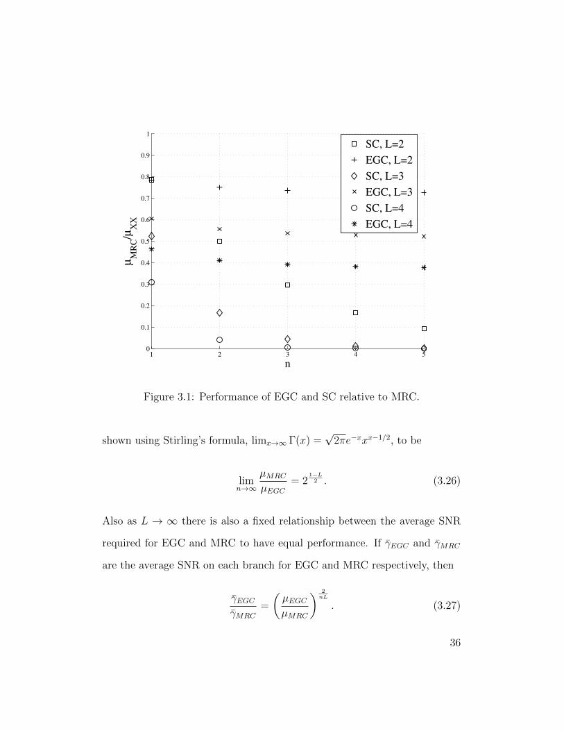
If we plot the µXX of SC and EGC relative to µMRC (the optimum linear

combiner), i.e. µMRC/µXX , as in Fig. 3.1, we see that for dual diversity (L=2)

and n = 1, SC and EGC achieve identical performance with µSC = µEGC =

4/π. This result has also been shown to apply at all SNRs for independent

Nagakami-m fading channels [41]. For L > 2 and n > 1 we see that EGC

is able to outperform SC while achieving similar performance to MRC. The

performance gap between both SC and EGC relative to MRC increases with

the number of branches and as the fading severity decreases.

Interestingly in Fig. 3.1, it appears as though as n → ∞, the ratio

µMRC/µEGC approaches a constant. This is indeed the case and can be

35

1 2 3 4 50

0.1

0.2

0.3

0.4

0.5

0.6

0.7

0.8

0.9

1µ

MR

C/µ

XX

n

SC, L=2

EGC, L=2

SC, L=3

EGC, L=3

SC, L=4

EGC, L=4

Figure 3.1: Performance of EGC and SC relative to MRC.

shown using Stirling’s formula, limx→∞ Γ(x) =√

2πe−xxx−1/2, to be

limn→∞

µMRC

µEGC= 2

1−L2 . (3.26)

Also as L → ∞ there is also a fixed relationship between the average SNR

required for EGC and MRC to have equal performance. If γEGC and γMRC

are the average SNR on each branch for EGC and MRC respectively, then

γEGCγMRC

=

(µEGCµMRC

) 2nL

. (3.27)

36

Again, using Sterling’s formula, we obtain

limL→∞

γEGCγMRC

=e

n21− 2n

[Γ(n)

Γ(n2

)] 2n

(3.28)

= 10 log10

(e

n21− 2n

)+

20

nlog10

(Γ(n)

Γ(n2

)) [dB]. (3.29)

This represents the additional power required at the transmitter if EGC is

implemented over MRC to reduce the combiner complexity. Similar results

for SC do not exist, with limn→∞ µMRC/µSC = 0 and limL→∞ γSC/γMRC =

∞.

3.5.2 Numerical Results

In order to validate our results we have plotted P∞e,c for BPSK and equal

average branch SNR along with Monte Carlo simulations in Fig. 3.2, Fig. 3.3,

and Fig. 3.4 for SC, EGC, and MRC respectively. In all cases we let λ =

[0.9, 0.3, 0.8]. We can see from Figs. 3.2-3.4 that for each combining method

the simulated results approach the asymptotic error rates as SNR increases.

37

0 5 10 15 20 25 3010

−9

10−8

10−7

10−6

10−5

10−4

10−3

10−2

10−1

BE

R

Average Branch SNR (dB)

n=1

n=2

n=3

Simulation

Figure 3.2: Asymptotic and simulated BERs of coherent BPSK of triplebranch SC with generalized Rician fading channels with S = 3 and λ =[0.9, 0.3, 0.8].

38

0 5 10 15 20 25 3010

−9

10−8

10−7

10−6

10−5

10−4

10−3

10−2

10−1

BE

R

Average Branch SNR (dB)

n=1

n=2

n=3

Simulation

Figure 3.3: Asymptotic and simulated BERs of coherent BPSK of triplebranch EGC with generalized Rician fading channels with S = 3 and λ =[0.9, 0.3, 0.8].

39

0 5 10 15 20 25 3010

−9

10−8

10−7

10−6

10−5

10−4

10−3

10−2

10−1

BE

R

Average Branch SNR (dB)

n=1

n=2

n=3

Simulation

Figure 3.4: Asymptotic and simulated BERs of coherent BPSK of triplebranch MRC with generalized Rician fading channels with S = 3 and λ =[0.9, 0.3, 0.8].

40

Chapter 4

Exact Series Form of the BER

with SC in Generalized Rician

Fading

In this chapter we develop an exact infinite series representation for the PDF

and CDF of the SNR for SC. The statistical distributions are then used to

obtain an exact infinite series expression for the BER of binary coherent and

noncoherent modulations. We also find an upper bound on the truncation

error introduced when the infinite series is truncated to a finite number of

terms.

4.1 Channel Model

Consider an L-branch diversity combiner where the transmitted signal is im-

paired by slow, frequency nonselective fading and AWGN on each branch.

The instantaneous SNR on the kth branch is γk = R2k, where Rk is a gen-

eralized Rician RV. Assume correlation among branches fits the generalized

41

correlation model, then the average SNR on the kth branch is γk = E[γk] =

σ2k

(n2

+ λ2kS

2)

and the power correlation between the kth and ith branch is

ργkγi =λ2kλ

2i (n2

+ 2S2)√n2

+ 2λ2kS

2√

n2

+ 2λ2iS

2, k 6= i (4.1)

as found in Chapter 2. Furthermore, let the average SNR of the kth branch

be given by γk = gkγ where gk is the gain of the kth branch relative to some

baseline SNR value γ. For instance, γ could be the average SNR across all

branches, in which case γ =∑L

k=1 γk.

4.2 SNR Distribution

We start by deriving an infinite series expression for the CDF at the output

of the SC combiner. Using the joint CDF of generalized Rician RVs with

generalized correlation (2.27), the CDF of γSC is given in single integral form

as

FγSC (γ) =FR (R1 ≤√γ,R2 ≤

√γ . . . , RL ≤

√γ) (4.2)

=exp (−S2)

Sn2−1

∞∫0

tn−2

4 exp (−t)In2−1(2S

√t)

×L∏k=1

[1−Qn

2

(√2λ2

kt

1− λ2k

,

√2dkγ

γ

)]dt. (4.3)

where dk =(n+2λ2

kS2)

2gk(1−λ2k)

.

42

A novel infinite series form of the generalized Marcum Q-function in

terms of generalized Laguerre polynomials was recently proposed by Andras

et al. [42] as

Qv(a, b) = 1−∞∑i=0

(−1)ie−a2

2

L(v−1)i

(a2

2

)Γ(v + i+ 1)

(b2

2

)v+i

. (4.4)

The availability of well known inequalities for the generalized Laguerre poly-

nomial makes this series suitable for a truncation error analysis. Substituting

(4.4) into (4.3) and interchanging the order of summation and integration we

can express FγSC (γ) as an infinite series

FγSC (γ) =

[L∏k=1

dk

]n2 ∞∑i=0

Ci

(γ

γ

)i+nL2

(4.5)

where the coefficient Ci is given by

Ci =(−1)i e−S

2

Sn2−1

∞∫0

tn−2

4 exp (− (Λ + 1) t) In2−1

(2S√t)

×∑

j1+···+jL=i

L∏k=1

L(n2−1)jk

(λ2kt

1−λ2k

)Γ(n

2+ jk + 1)

djkk dt. (4.6)

To evaluate the integral in Ci we consider the integral identity

∞∫0

ti+µ−1

2 e−αtIµ−1

(2β√t)dt = i!

(β

αi

)µexp

(β2

α

)L

(µ−1)i

(−β

2

α

)(4.7)

43

where i ∈ N and µ > 0. The derivation of (4.7) is located in Appendix B.

The integral in Ci can then be evaluated using a finite series form of the

generalized Laguerre polynomial [39, Eq. (22.3.9)]

L(α)i (x) =

i∑j=0

(j + α + 1)i−j(i− j)!j!

(−x)j, α > −1 (4.8)

and the integral identity (4.7) along with some algebraic simplifications to

obtain

Ci =(−1)i e−

ΛΛ+1

S2

(Λ + 1)n2 ΓL

(n2

) ∑j1+···+jL=i

L∏k=1

djkkjk!(n2

+ jk)

×j1,...,jL∑

l1=0,...,lL=0

(∑Lk=1 lk

)!

(Λ + 1)∑Lk=1 lk

L(n2−1)∑Lk=1 lk

(− S2

1 + Λ

)

×L∏k=1

(jklk

)1(n2

)lk

(−λ2

k

1− λ2k

)lk. (4.9)

The PDF of γSC can be found by differentiating (4.5) w.r.t. γ, upon

which we obtain

fγSC (γ) =

[L∏k=1

dk

]n2 ∞∑i=0

(nL

2+ i

)Ciγ

(γ

γ

)i+nL2−1

. (4.10)

It is easy to verify that the first term in (4.10) is the asymptotic PDF at the

output of the SC combiner (3.12) derived in Chapter 3.

As a sanity check, we examine the special case when L = 1. For L = 1,

44

Ci is simplifies to

Ci =(−d)i(1− λ2)

n2

+ie−λ2S2

Γ(n2

)i!(n2

+ i) i∑

l=0

(i

l

)(1 +

λ2

1− λ2

)i−l( −λ2

1− λ2

)l

× L(n2−1)l (−(1− λ2)S2)

L(n2−1)l (0)

=(−d)i(1− λ2)

n2

+ie−λ2S2

Γ(n2

)i!(n2

+ i) L

(n2−1)i (λ2S2)

L(n2−1)i (0)

(4.11)

where we have used the fact that L(α)n (0) = (α+1)n

n!and a Laguerre sum

formula [43, Eq. (18.18.12)]. Substituting (4.11) into (4.10) we obtain the

following

fγSC (γ) =e−λ

2S2

Γ(n2

)σ2

( γσ2

)n2−1

∞∑i=0

(− γ

σ2

)i L(n2−1)i (λ2S2)

i!L(n2−1)i (0)

(4.12)

=γn−2

4 e−λ2S2− γ

σ2

σ2 (λSσ)n2−1

In2−1

(2λS

σ

√γ

)(4.13)

where we have used the formula [42]

∞∑i=0

L(α)i (x)

L(α)i (0)

(−z)i

i!= Γ(α + 1)e−z(xz)−

α2 Iα(2

√xz). (4.14)

This matches the result found by differentiating (4.2) w.r.t. γ, substituting

(2.29) and letting L = 1.

45

4.3 BER of Binary Modulations

4.3.1 BER for Binary Coherent Modulations

For binary coherent modulations, the conditional error rate is given by

Pe|γ = Q (√qγ) . (4.15)

where q = 2 for BPSK and q = 1 for binary coherent frequency shift keying

(BCFSK). Substituting (4.15) into (3.2) and changing the order of integration

we obtain

Pe,c =1√2π

∞∫0

exp

(−x

2

2

)Fγ

(x2

q

)dx. (4.16)

An infinite series form for Pe,c can then be found by substituting (4.5)

into (4.16) and changing the order of summation and integration to arrive at

Pe,c =1

2√π

[L∏k=1

dk

]n2 ∞∑i=0

2nL2

+iCiΓ(i+ nL+1

2

)(γq)

nL2

+i. (4.17)

As γ →∞, Eq. (4.17) is dominated by the first term in the summation:

Pe,c ≈1

2√π

L∏k=1

(n+ 2λ2

kS2

2gk

)n2 (−1)i e−

ΛΛ+1

S2

Γ(nL+1

2

)(Λ + 1)

n2 ΓL

(n2

+ 1) 1

γnL2

(4.18)

which matches the asymptotic BER (3.4) when t and a are given by (3.14)

and (3.13) respectively.

Although we have only derived the BER of coherent binary modulations,

46

the results can be generalized to many M -ary linear digital modulations

following an MGF approach [1].

4.3.2 BER for Binary Noncoherent Modulations

As mentioned in Chapter 3, the conditional error rate for binary noncoherent

modulations is given by Pe|γ = 12

exp (−qγ), where q = 1/2 for BNCFSK and

q = 1 for BDPSK. We then obtain the average BER as

Pe,nc =1

2

∞∫0

exp (−qγ) fγ (γ) dγ. (4.19)

Substituting (4.10) into (4.19) and changing the order of integration we ob-

tain an infinite series solution for the BER

Pe,nc =1

2

[L∏k=1

dk

]n2 ∞∑i=0

CiΓ(i+ nL

2+ 1)

(γq)nL2

+i. (4.20)

4.4 Convergence and Truncation Error

4.4.1 Convergence

Thus far, we have proceeded with interchanging the order of summation

and integration without considering whether the resulting series converges

or not. While we will show the infinite series forms of FγSC (γ) and fγSC (γ)

are convergent for all 0 ≤ γ < ∞, the infinite series for the BER for both

47

coherent and noncoherent modulations are only convergent for a sufficiently

high average SNR.

We start by finding an upper bound on Ci. To achieve this, we return to

the form of Ci prior to carrying out the integration (4.6), and apply a well

known inequality for the generalized Laguerre polynomial [39, Eq. (22.14.13)]

∣∣∣L(α)i (x)

∣∣∣ ≤ (α + 1)ii!

exp(x

2

), α ≥ 0, x ≥ 0 (4.21)

along with an integral identity [37, Eq. (3.15.2.8)] to obtain

|Ci| ≤exp

(− ΛS2

(Λ+2)

)ΓL(n2

) (Λ2

+ 1)n

2

∑j1+···+jL=i

L∏k=1

djkk(n2

+ jk)jk!

≤exp

(− ΛS2

(Λ+2)

)ΓL(n2

+ 1) (

Λ2

+ 1)n

2

∑j1+···+jL=i

L∏k=1

djkkjk!

=exp

(− ΛS2

(Λ+2)

)ΓL(n2

+ 1) (

Λ2

+ 1)n

2

ηi

i!(4.22)

where η =∑L

k=1 dk and we have used the multinomial identity to get (4.22).

Note that due to the use of (4.21), which is valid only for α ≥ 0, Eq. (4.22)

applies for n > 1 only. For n = 1 we use the inequality

∣∣∣L(α)i (x)

∣∣∣ ≤ 2 exp(x

2

)− 1 < α ≤ 0, x ≥ 0 (4.23)

which is a relaxed form of [39, Eq. (22.14.14)]. Using a similar methodology

48

to how (4.25) was obtained, we find for n = 1

|Ci| ≤2L exp

(− ΛS2

(Λ+2)

)√

Λ2

+ 1

∑j1+···+jL=i

L∏k=1

djkkΓ(jk + 3

2)

≤2L exp

(− ΛS2

(Λ+2)

)√

Λ2

+ 1

∑j1+···+jL=i

L∏k=1

djkkjk!

=2L exp

(− ΛS2

(Λ+2)

)√

Λ2

+ 1

ηi

i!. (4.24)

Since (4.22) and (4.24) vary only by a constant coefficient, we define a new

term valid for all n = 1, 2, . . .

|Ci| ≤ Aηi

i!(4.25)

A =

2 exp

(− ΛS2

(Λ+2)

)πL2 (Λ

2+1)

n2

n = 1

exp(− ΛS2

(Λ+2)

)ΓL(n2 +1)(Λ

2+1)

n2

n = 2, 3, . . .

. (4.26)

Using (4.25), we can now bound the series form of FγSC (γ) (4.5) as follows

|FγSC (γ)| ≤

[L∏k=1

dk

]n2 ∞∑i=0

|Ci|(γ

γ

)i+nL2

≤ A

(γ

γ

)nL2

[L∏k=1

dk

]n2 ∞∑i=0

1

i!

(ηγ

γ

)i

= A

(γ

γ

)nL2

[L∏k=1

dk

]n2

exp

(ηγ

γ

). (4.27)

49

Eq. (4.27) converges for 0 ≤ γ <∞, thus convergence of (4.5) is guaranteed

for the same interval. A similar exercise can be performed to show that the

PDF in (4.10) also converges for 0 ≤ γ <∞.

Due to the presence of the Γ(·) term in the numerator of the summation

in (4.17), convergence of the series is conditional. Finding the entire region

of convergence of (4.17) is extremely complex due to the nested summations.

However, we can find a subset of the region of convergence using the upper

bound on |Ci|. Using (4.25), we find

|Pe,c| ≤2nL2−1A

√π(qγ)

nL2

[L∏k=1

dk

]n2 ∞∑i=0

Γ(i+ (nL+1)

2

)i!

(2η

qγ

)i(4.28)

which converges by the ratio test for 2ηqγ< 1. Similarly, it can be shown (4.20)

converges when ηqγ< 1.

The requirement 2ηqγ

< 1 or ηqγ

< 1 is satisfied provided that average

branch power is sufficiently high. For instance, for branches experiencing

equally correlated Nakagami-m fading, equal average branch SNR, and BPSK

modulation we require ηγ< 1, which is achieved when γ > mL

(1−√ρ)where

ρ = λ4 is the power correlation coefficient between any two branches. From

this we can infer that the minimum γ required to guarantee the infinite series

expressions for Pe converge increases with the number of branches and branch

correlation, but decreases with the fading severity.

50

4.4.2 Truncation Error

In this section we derive an upper bound on the truncation errors when

the infinite series for SNR CDF (4.5) and BER for binary coherent mod-

ulations (4.17) are terminated at a finite number of terms. We omit the

results for binary noncoherent modulations, but the truncation error can be

bounded in a similar manner.

The truncation of (4.5) and (4.17) and to the first N + 1 terms is given

by

F (N)γSC

(γ) =

[L∏k=1

dk

]n2 N∑i=0

Ci

(γ

γ

)i+nL2

(4.29)

P (N)e,c =

1

2√π

[L∏k=1

dk

]n2 N∑i=0

2nL2

+iCiΓ(i+ nL+1

2

)(qγ)

nL2

+i. (4.30)

We then define the associated truncation errors as ε(N)FγSC

(γ) ,∣∣∣FγSC (γ)− F (N)

γSC (γ)∣∣∣

and ε(N)Pe,c

(γ) ,∣∣∣Pe,c(γ)− P (N)

e,c (γ)∣∣∣ respectively. ε

(N)FγSC

(γ) can be bounded us-

ing (4.25) to obtain

ε(N)FγSC

(γ) ≤A(γ

γ

)nL2

[L∏k=1

dk

]n2 ∞∑i=N+1

1

i!

(ηγ

γ

)i(4.31)

=A

(γ

γ

)nL2

[L∏k=1

dk

]n2

exp

(ηγ

γ

)i−

N∑i=0

1

i!

(ηγ

γ

)i. (4.32)

51

Likewise we bound ε(N)Pe,c

(γ) as

ε(N)Pe,c≤ 2

nL2−1A

√π(qγ)

nL2

[L∏k=1

dk

]n2 ∞∑i=N+1

Γ(i+ nL+1

2

)i!

(2η

qγ

)i(4.33)

=2nL2−1Γ

(nL+1

2

)A

√π(qγ)

nL2

[L∏k=1

dk

]n2

1(1− 2η

qγ

)nL+12

−N∑i=0

(nL+1

2

)i

i!

(2η

qγ

)i(4.34)

where we have used the binomial series 1(1−x)α

=∑∞

i=0(α)ii!xi, |x| < 1 to

obtain (4.34). It is easy to see from (4.33) that the upper bound on the

truncation error is o(γ−(nL2 +N+2)

), the same order as the first term ignored

when the series is truncated to (4.30). Thus, we can conclude our truncation

error bound decreases relative to the truncated error rate as γ →∞.

4.5 Numerical Results

In order to verify that (4.30) converges to the exact error rate, we have

plotted it for BPSK with N = 30 along with Monte Carlo simulations for

Nakagami-m (m = 2) and Rician (S = 1.5) fading with equal average branch

SNR in Fig. 4.1. In both cases we have used λ = [0.6, 0.4, 0.9], resulting in

52

power correlation matrices, where the (k, i)th element is given by (4.1), of

P1 =

1 0.149 0.460

0.149 1 0.252

0.460 0.252 1

(4.35)

and

P2 =

1 0.058 0.292

0.058 1 0.130

0.292 0.130 1

(4.36)

for Rician and Nagakami-m respectively. We see fem Fig. 4.1 that in both

cases, the approximation is highly accurate where the series converges. The

convergence criterion for BPSK, ηγ< 1, is satisfied when γ > 12.85 dB for

Rician fading and γ > 12.05 dB for Nakagami-m fading. This is very close to

the true value for the Nakagami-m fading; however, the convergence region

of Rician fading is underestimated by roughly 2 dB.

Although we have chosen N = 30 in the previous example, the asymptotic

error rate can be greatly improved by including only a couple extra terms.

This is shown in Fig. 4.2, where we have replotted the asymptotic (N = 0)

error rate along with N = 1 and N = 2 for Rician fading. The parameters

are the same as the for the Rician case in Fig. 4.1. The asymptotic error rate

is not within 1% of the exact error rate until 28.9 dB. By adding a single

additional term this occurs at 18.5 dB, and two additional terms improves it

further to 14.8 dB. Thus, we can extend the SNR region where the asymptotic

53

expression is valid with little additional complexity by including the first

several terms of the infinite series.

Fig. 4.3 shows the relative truncation error for Nakagami-2 fading, where

the relative truncation error is the ratio of (4.34) to (4.30). As we would

expect, the number of terms required to satisfy a truncation error target di-

minishes as SNR increases. For instance, to guarantee a relative truncation

error less than 1%, we require N = 40 at 14.3 dB, but this drops to N = 10

at 17.4 dB, and further to N = 5 at 19.7 dB. Although it is tempting to

increase N to achieve an arbitrary accuracy, computation of CN can be very

intensive for large N and numerical integration of (4.16) may be more effi-

cient. However, it should be noted that provided the relative SNRs between

branches remains constant, Ci, i = 1, 2, . . . , N need only be computed once,

whereas numerical integration would have to be performed at each SNR.

54

11 12 13 14 15 16 17 18 19 2010

−9

10−8

10−7

10−6

10−5

10−4

10−3

10−2

BE

R

Average Branch SNR (dB)

Approx Rician

Approx Nakagami

Simulation

Figure 4.1: Approximate (N = 30) and simulated BERs of coherent BPSKof triple branch SC with Rician and Nakagami-m fading. Average SNR isidentical for each branch. For Rician fading, S = 1.5 and for Nakagami-m, m = 2. Power correlation is according to P1 and P2 for Rician andNakagami-m, respectively.

55

9 10 11 12 13 14 15 16 17 18 19 2010

−6

10−5

10−4

10−3

10−2

BE

R

Average Branch SNR (dB)

N=0

N=1

N=2

Simulation

Figure 4.2: Approximate and simulated BERs of coherent BPSK of triplebranch SC with Rician fading (S = 1.5) and equal average branch SNR.Branches are correlated with power correlation matrix P1.

56

10 15 20 25 30 35 4010

−6

10−5

10−4

10−3

10−2

10−1

100

101

102

Up

per

Bo

un

d o

n t

he

Rel

ativ

e T

run

cati

on

Err

or

Average Branch SNR (dB)

N=0

N=2

N=5

N=10

N=20

N=40

Figure 4.3: Relative truncation error for coherent BPSK with triple branchSC in Nakagami-2 fading and equal average branch SNR. Branches are cor-related with power correlation matrix P2.

57

Chapter 5

Asymptotically Tight Error

Bounds for EGC with

Generalized Rician Fading

In this chapter, we derive single integral upper and lower bounds on the

average error rate of a receiver employing EGC in correlated generalized

Rician fading. These bounds are asymptotically exact, i.e. as average SNR

approaches infinity. Furthermore, the bounds reduce to the exact error rate

when the branches are independent.

5.1 Channel Model

Consider an L-branch diversity combiner where the transmitted signal is im-

paired by slow, frequency nonselective fading and AWGN on each branch.

The instantaneous SNR on the kth branch is γk = R2k, where Rk is a gen-

eralized Rician RV. Assume correlation among branches fits the generalized

correlation model, then the average SNR on the kth branch is γk = E[γk] =

58

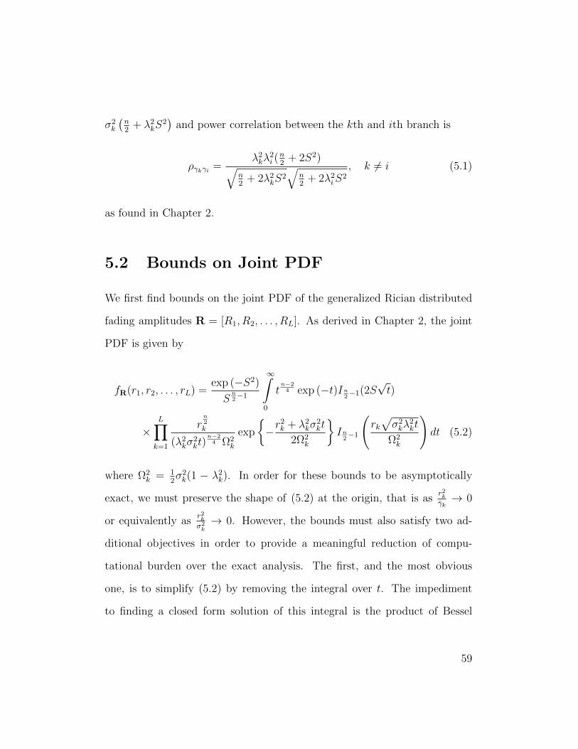
σ2k

(n2

+ λ2kS

2)

and power correlation between the kth and ith branch is

ργkγi =λ2kλ

2i (n2

+ 2S2)√n2

+ 2λ2kS

2√

n2

+ 2λ2iS

2, k 6= i (5.1)

as found in Chapter 2.

5.2 Bounds on Joint PDF

We first find bounds on the joint PDF of the generalized Rician distributed

fading amplitudes R = [R1, R2, . . . , RL]. As derived in Chapter 2, the joint

PDF is given by

fR(r1, r2, . . . , rL) =exp (−S2)

Sn2−1

∞∫0

tn−2

4 exp (−t)In2−1(2S

√t)

×L∏k=1

rn2k

(λ2kσ

2kt)

n−24 Ω2

k

exp

−r

2k + λ2

kσ2kt

2Ω2k

In

2−1

(rk√σ2kλ

2kt

Ω2k

)dt (5.2)

where Ω2k = 1

2σ2k(1 − λ2

k). In order for these bounds to be asymptotically

exact, we must preserve the shape of (5.2) at the origin, that is asr2k

γk→ 0

or equivalently asr2k

σ2k→ 0. However, the bounds must also satisfy two ad-

ditional objectives in order to provide a meaningful reduction of compu-

tational burden over the exact analysis. The first, and the most obvious

one, is to simplify (5.2) by removing the integral over t. The impediment

to finding a closed form solution of this integral is the product of Bessel

59

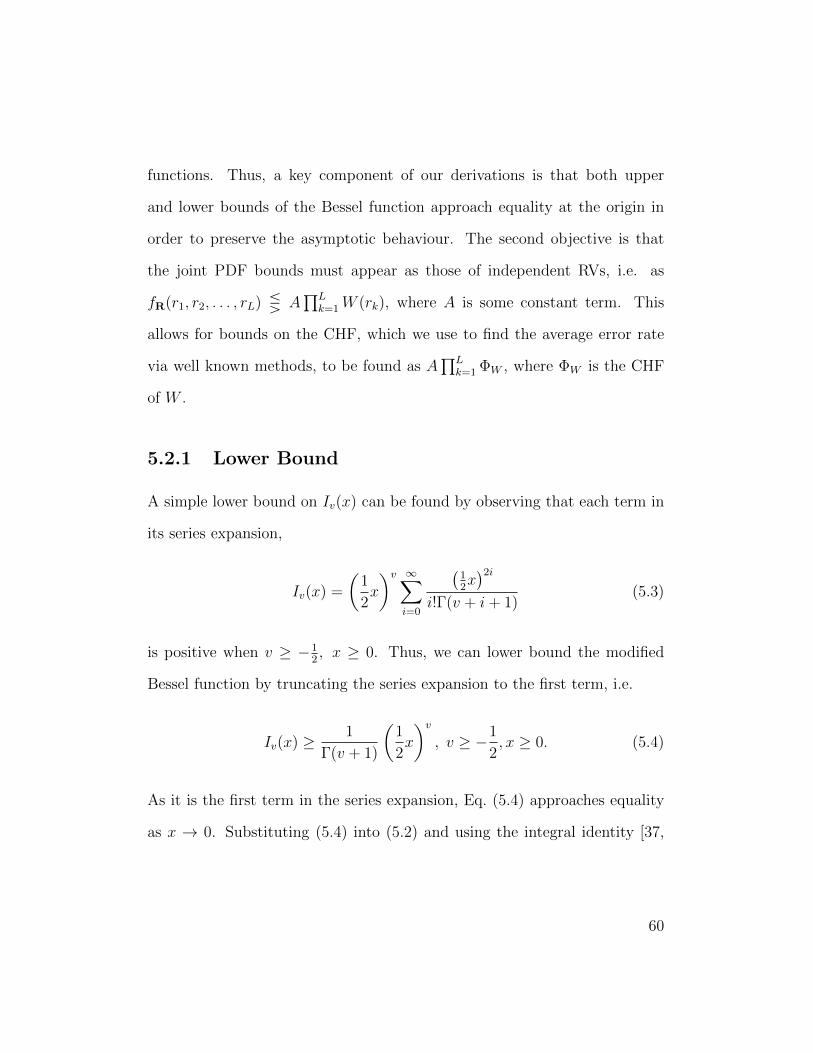
functions. Thus, a key component of our derivations is that both upper

and lower bounds of the Bessel function approach equality at the origin in

order to preserve the asymptotic behaviour. The second objective is that

the joint PDF bounds must appear as those of independent RVs, i.e. as

fR(r1, r2, . . . , rL) Q A∏L

k=1W (rk), where A is some constant term. This

allows for bounds on the CHF, which we use to find the average error rate

via well known methods, to be found as A∏L

k=1 ΦW , where ΦW is the CHF

of W .

5.2.1 Lower Bound

A simple lower bound on Iv(x) can be found by observing that each term in

its series expansion,

Iv(x) =

(1

2x

)v ∞∑i=0

(12x)2i

i!Γ(v + i+ 1)(5.3)

is positive when v ≥ −12, x ≥ 0. Thus, we can lower bound the modified

Bessel function by truncating the series expansion to the first term, i.e.

Iv(x) ≥ 1

Γ(v + 1)

(1

2x

)v, v ≥ −1

2, x ≥ 0. (5.4)

As it is the first term in the series expansion, Eq. (5.4) approaches equality

as x → 0. Substituting (5.4) into (5.2) and using the integral identity [37,

60

Eq. (3.15.2.8)] we obtain

fR(r1, . . . , rL) ≥ e−Λ

Λ+1S2

detn2 (M)

L∏k=1

2rn−1k

Γ(n2

)σnke− r2k

2Ω2k (5.5)

where Λ =∑L

k=1

λ2k

1−λ2k

and the matrix M is defined in (3.9). Eq. (5.5) satisfies

both our objectives, and thus it is a suitable lower bound.

For the special case of Nakagami-m fading, we note that (5.5) is a scaled

product of Nakagami-m PDFs

fR(r1, . . . , rL) ≥ 1

(1 + Λ)m

L∏k=1

21−mr2m−1k

Γ (m) Ω2mk

e− r2k

2Ω2k (5.6)

and thus the equality is also achieved for independent branches since Λ = 0.

5.2.2 Upper Bound

While derivation of a suitable lower bound of the joint PDF is straightfor-

ward, this is not the case for the upper bound. We start by considering an

upper bound on the Bessel function of the first kind [39, Eq. (9.1.62)]

|Jv(x)| ≤ exp |=(x)|Γ(v + 1)

∣∣∣∣12x∣∣∣∣ , v ≥ −1

2. (5.7)

Using the relation Iv(x) = j−vJv(jx), where j2 = −1, we obtain for x ∈ R

Iv(x) ≤ exp(x)

Γ(v + 1)

(1

2x

)v, v ≥ −1

2, x ≥ 0 (5.8)

61

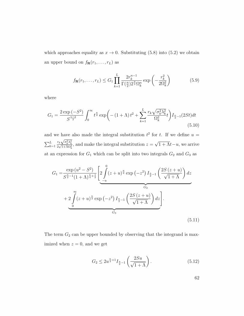
which approaches equality as x→ 0. Substituting (5.8) into (5.2) we obtain

an upper bound on fR(r1, . . . , rL) as

fR(r1, . . . , rL) ≤ G1

L∏k=1

2rn−1k

Γ(n2)2

n2 Ωn

k

exp

(− r2

k

2Ω2k

)(5.9)

where

G1 =2 exp (−S2)

Sn−2

2

∫ ∞0

tn2 exp

(− (1 + Λ) t2 +

L∑k=1

rk√σ2kλ

2k

Ω2k

t

)In

2−1(2St)dt

(5.10)

and we have also made the integral substitution t2 for t. If we define u =∑Lk=1

rk√σ2kλ

2k

2√

1+ΛΩ2k

, and make the integral substitution z =√

1 + Λt−u, we arrive

at an expression for G1 which can be split into two integrals G2 and G3 as

G1 =exp (u2 − S2)

Sn2−1(1 + Λ)

n4

+ 12

[2

0∫−u

(z + u)n2 exp

(−z2

)In

2−1

(2S (z + u)√

1 + Λ

)dz

︸ ︷︷ ︸G2

+ 2

∞∫0

(z + u)n2 exp

(−z2

)In

2−1

(2S (z + u)√

1 + Λ

)dz

︸ ︷︷ ︸G3

].

(5.11)

The term G2 can be upper bounded by observing that the integrand is max-

imized when z = 0, and we get

G2 ≤ 2un2

+1In2−1

(2Su√1 + Λ

). (5.12)

62

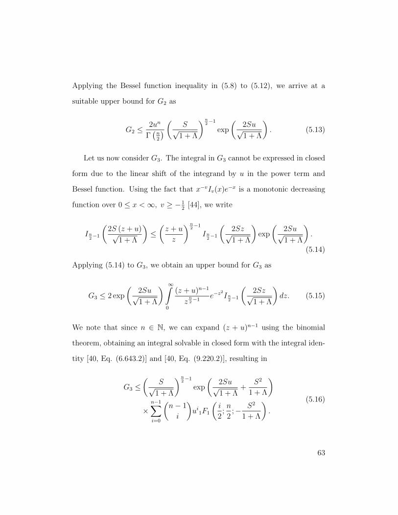
Applying the Bessel function inequality in (5.8) to (5.12), we arrive at a

suitable upper bound for G2 as

G2 ≤2un

Γ(n2

) ( S√1 + Λ

)n2−1

exp

(2Su√1 + Λ

). (5.13)

Let us now consider G3. The integral in G3 cannot be expressed in closed

form due to the linear shift of the integrand by u in the power term and

Bessel function. Using the fact that x−vIv(x)e−x is a monotonic decreasing

function over 0 ≤ x <∞, v ≥ −12

[44], we write

In2−1

(2S (z + u)√

1 + Λ

)≤(z + u

z

)n2−1

In2−1

(2Sz√1 + Λ

)exp

(2Su√1 + Λ

).

(5.14)

Applying (5.14) to G3, we obtain an upper bound for G3 as

G3 ≤ 2 exp

(2Su√1 + Λ

) ∞∫0

(z + u)n−1

zn2−1

e−z2

In2−1

(2Sz√1 + Λ

)dz. (5.15)

We note that since n ∈ N, we can expand (z + u)n−1 using the binomial

theorem, obtaining an integral solvable in closed form with the integral iden-

tity [40, Eq. (6.643.2)] and [40, Eq. (9.220.2)], resulting in

G3 ≤(

S√1 + Λ

)n2−1

exp

(2Su√1 + Λ

+S2

1 + Λ

)×

n−1∑i=0

(n− 1

i

)ui1F1

(i

2;n

2;− S2

1 + Λ

).

(5.16)

63

The results in (5.13) and (5.16) allow us to find an upper bound on G1 as

G1 ≤1

(1 + Λ)n2

exp

(u2 +

2Su√1 + Λ

− ΛS2

1 + Λ

)[ n∑i=0

aiui

](5.17)

ai =

(n−1i

)1F1

(i2; n

2;− S2

1+Λ

)i = 0, . . . , n− 1

2

Γ(n2 )exp

(−S2

1+Λ

)i = n

. (5.18)

Although we have found an upper bound for G1 which is in the desired closed

form, we cannot partition (5.17) into a product of L independent functions.

Since ui for i ∈ N, u ≥ 0 is a convex function we can obtain, via Jensen’s

inequality, the following

(L∑k=1

rk√σ2kλ

2k

2√

1 + ΛΩ2k

)i

≤L∑k=1

λ2k

Λ (1− λ2k)

(Λrk√

(1 + Λ) σ2kλ

2k

)i

. (5.19)

Eq. (5.19), when combined with the inequality 1 +∑N

k=1 bk ≤∏N

k=1(1 +

bk), bk ≥ 0, allows us to find a suitable upper bound for G1 as

G1 ≤exp

(− Λ

Λ+1S2)

(1 + Λ)n2

L∏k=1

exp

(Λ

1 + Λ

r2k

2Ω2k

+S

1 + Λ

rk√λ2kσ

2k

Ω2k

)

×

1 +λ2k

Λ (1− λ2k)

n∑i=1

ai

(Λrk√

1 + Λ√σ2kλ

2k

)i . (5.20)

Finally, by substituting (5.20) into (5.9) we obtain the upper bound of joint

64

PDF of the generalized Rician distribution as

fR(r1, . . . , rL)

≤exp

(− Λ

Λ+1S2)

(1 + Λ)n2 ΓL

(n2

) L∏k=1

1 +λ2k

Λ (1− λ2k)

n−1∑i=1

ai

(Λrk√

1− λ2k√

1 + Λ√

2Ω2kλ

2k

)i

× 2rn−1k

2n2 Ωn

k

exp

(− 1

1 + Λ

r2k

2Ω2k

+S

1 + Λ

rk√λ2kσ

2k

Ω2k

). (5.21)

As in the case with the lower bound of the joint PDF, by letting λk = 0, k =

1, . . . , L, we can show the equality in (5.21) is obtained for the Nakagami-m

fading with independent branches.

5.3 Error Bounds

In this section we use the lower and upper bounds on the joint PDF in (5.5)

and (5.21) respectively, to bound the error rate of an EGC combiner. As in

Chapter 3, we perform error analysis on the equivalent channel at the output

of the combiner hEGC =√γEGC = 1

L

∑Lk=1 Rk.

An alternate equation for the average error probability can be found by

applying Parseval’s theorem to (3.2) [45]:

Pe =1

π

∞∫0

<G∗ (ω) ΦhEGC (ω) dω (5.22)

where ΦhEGC (ω) is the CHF of hEGC and G (ω) is the Fourier transform of

65

the conditional error probability. A full list of G(ω) for various coherent and

noncoherent modulations is given in [Table 1][45]. For example, G(ω) for

BPSK is given by

G (ω) =1

2ω

2√πF(ω

2

)+ j

[1− exp

(−ω

2

4

)]. (5.23)

It is apparent that using upper or lower bounds on ΦhEGC (ω) in the

integration of (5.22) results in upper or lower bounds on Pe as

Pe ≥ Pe,L =1

π

∞∫0

<G∗ (ω) ΦhEGC ,L (ω) dω (5.24)

Pe ≤ Pe,H =1

π

∞∫0

<G∗ (ω) ΦhEGC ,H (ω) dω (5.25)

where ΦhEGC ,L (ω) and ΦhEGC ,H (ω) are the upper and lower bounds respec-

tively on ΦhEGC (ω) found using (5.5) and (5.21). From the definition of the

CHF we have

ΦhEGC (ω) =

∞∫0

· · ·∞∫

0︸ ︷︷ ︸L

ej ω√

L

∑Lk=1 rkfR(r1, r2, . . . , rL)dr1dr2 · · · rL. (5.26)

In both cases, substituting (5.5) or (5.21) into (5.26) to find ΦhEGC ,L (ω) or

66

ΦhEGC ,H (ω), respectively requires integral identity

∞∫0

xn+i−1

αn+iΓ(n)exp

(− x2

2α2+ βx

)dx = (n)i D−n−i (−αβ) (5.27)

which can be found from [40, Eq. (3.462.1)]. Here in (5.27), D−n (z) is the

normalized parabolic cylinder function2 and can be expressed in terms of the

confluent hypergeometric function using [40, Eq. (9.240)]

D−n (z) =1

2n2

[ √π

Γ(n+1

2

)1F1

(n

2;1

2;z2

2

)−√

2πz

Γ(n2

) 1F1

(n+ 1

2;3

2;z2

2

)]. (5.28)

From (5.5) we obtain the lower bound of the characteristic function

ΦhEGC ,L(ω) =exp

(− Λ

Λ+1S2)

(1 + Λ)n2

(Γ(n+1

2

)2n2

√π

)L L∏k=1

D−n

(−jωΩk√

L

)(5.29)

and from (5.21), we obtain the upper bound of the characteristic function

ΦhEGC ,H(ω) =exp

(− Λ

Λ+1S2)

(1 + Λ)(1−L)n2

(2n2 Γ(n+1

2

)√π

)L L∏k=1

[D−n (−βk)

+λ2k

Λ (1− λ2k)

n∑i=1

(Λ√

1− λ2k√

λ2k

)iai (n)i

2i2

D−n−i (−βk)

](5.30)

where βk = S√1+Λ

√2λ2k

1−λ2k

+ jωΩk

√1+ΛL

. We have made use of the Gauss

duplication formula [40, Eq. (8.335.1)] in the derivation of (5.29) and (5.30).

2Dp (z) is related to the parabolic cylinder function, Dp (z), in [40] by Dp (z) =

e−z2

4 Dp (z). We have elected to use this alternate notation for simplicity.

67

Both error bounds, (5.24) and (5.25), consist of a single integral of closed

form functions with implementations in popular mathematical software. There-

fore, they are similar in computational complexity to the exact analysis for

independent branches found in [45] and far simpler than the exact results

in [22] and [46] which use the generalized correlation model with λk = λ, k =

1, 2 . . . , L, i.e. equally correlated branches.

5.4 Numerical Results

The upper and lower bounds we have developed, in addition to being asymp-

totically tight for correlated fading, are exact for independent fading. Thus

we expect the bounds to be tighter for weaker correlation among branches.

We can see this is indeed the case by comparing Fig. 5.1 and Fig. 5.2 which

plot Pe,L and Pe,H along with the asymptotic results found in Chapter 3

for Rayleigh fading channels with coherent BPSK and equal average branch

SNRs. The numerical results in Fig. 5.1 and Fig. 5.2 have power correlation

matrices, where the (k, i)th element is given by (5.1), of

P1 =

1 0.518 0.656

0.518 1 0.518

0.656 0.518 1

(5.31)

68

and

P2 =

1 2.25× 10−2 2.03× 10−1

2.25× 10−2 1 7.29× 10−2

2.03× 10−1 7.29× 10−2 1

(5.32)

respectively. We observe that while both bounds approach simulation results

asymptotically, the lower bound is a much tighter fit especially at the higher

correlation of P2 in Fig. 5.1.

Additional scenarios with Nakagami-m and Rician fading channels are

shown in Fig. 5.3 and Fig. 5.4 with power correlation matrices

P3 =

1 3.5× 10−3 1× 10−2

3.5× 10−3 1 2.25× 10−2

1× 10−2 2.25× 10−2 1

(5.33)

and

P4 =

1 0.174 0.237

0.174 1 0.138

0.237 0.138 1

(5.34)

respectively.

We can see in Figs. 5.1-5.4, that while both bounds approach simulation

results asymptotically, the lower bound is a much tighter fit especially at

higher correlation. This is to be expected given the extra inequalities needed

to produce a suitable upper bound. In situations were the SER-SNR curve

is concave, as is the case in Figs. 5.1-5.4, the asymptotic error rate approx-

69

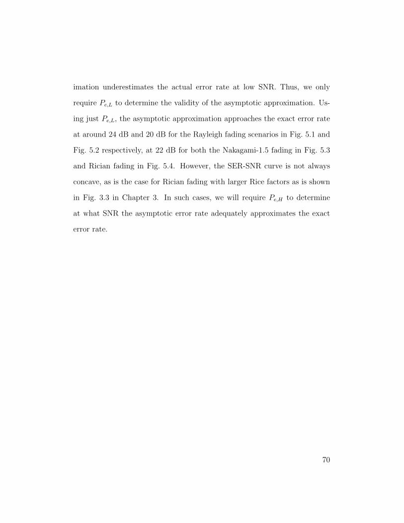
imation underestimates the actual error rate at low SNR. Thus, we only

require Pe,L to determine the validity of the asymptotic approximation. Us-

ing just Pe,L, the asymptotic approximation approaches the exact error rate

at around 24 dB and 20 dB for the Rayleigh fading scenarios in Fig. 5.1 and

Fig. 5.2 respectively, at 22 dB for both the Nakagami-1.5 fading in Fig. 5.3

and Rician fading in Fig. 5.4. However, the SER-SNR curve is not always

concave, as is the case for Rician fading with larger Rice factors as is shown

in Fig. 3.3 in Chapter 3. In such cases, we will require Pe,H to determine

at what SNR the asymptotic error rate adequately approximates the exact

error rate.

70

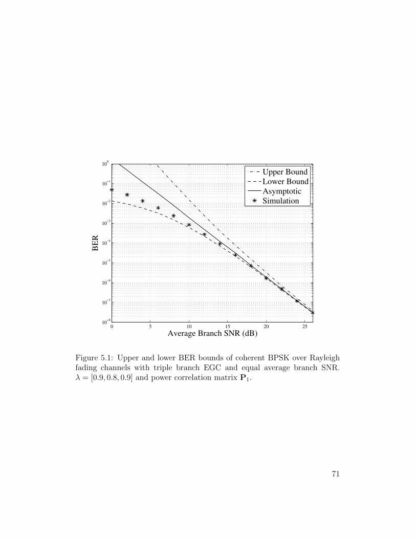
0 5 10 15 20 2510

−8

10−7

10−6

10−5

10−4

10−3

10−2

10−1

100

BE

R

Average Branch SNR (dB)

Upper Bound

Lower Bound

Asymptotic

Simulation

Figure 5.1: Upper and lower BER bounds of coherent BPSK over Rayleighfading channels with triple branch EGC and equal average branch SNR.λ = [0.9, 0.8, 0.9] and power correlation matrix P1.

71

0 5 10 15 20 2510

−8

10−7

10−6

10−5

10−4

10−3

10−2

10−1

100

BE

R

Average Branch SNR (dB)

Upper Bound

Lower Bound

Asymptotic

Simulation

Figure 5.2: Upper and lower BER bounds of coherent BPSK over Rayleighfading channels with triple branch EGC and equal average branch SNR.λ = [0.5, 0.3, 0.8] and power correlation matrix P2.

72

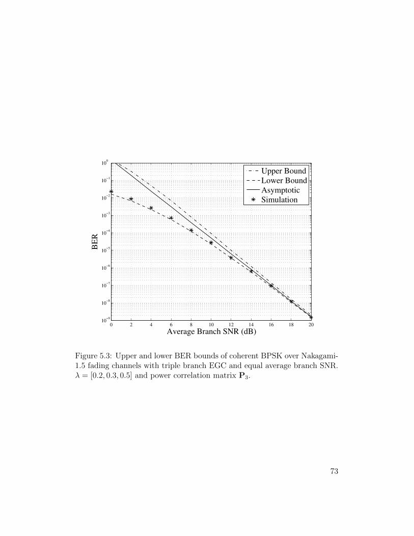
0 2 4 6 8 10 12 14 16 18 2010

−9

10−8

10−7

10−6

10−5

10−4

10−3

10−2

10−1

100

BE

R

Average Branch SNR (dB)

Upper Bound

Lower Bound

Asymptotic

Simulation

Figure 5.3: Upper and lower BER bounds of coherent BPSK over Nakagami-1.5 fading channels with triple branch EGC and equal average branch SNR.λ = [0.2, 0.3, 0.5] and power correlation matrix P3.

73

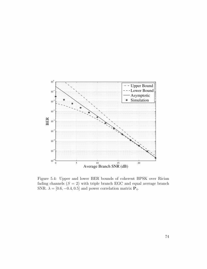
0 5 10 15 2010

−8

10−7

10−6

10−5

10−4

10−3

10−2

10−1

100

BE

R

Average Branch SNR (dB)

Upper Bound

Lower Bound

Asymptotic

Simulation

Figure 5.4: Upper and lower BER bounds of coherent BPSK over Ricianfading channels (S = 2) with triple branch EGC and equal average branchSNR. λ = [0.6,−0.4, 0.5] and power correlation matrix P4.

74

Chapter 6

Conclusion

6.1 Summary of Results

In this thesis we derived methods for improving and/or bounding the asymp-

totic error rates of SC and EGC over correlated generalized Rician fading

channels. We first derived asymptotic error rates for SC, EGC, and MRC

and compared their relative performance. The asymptotic results for SC were

then extended into an exact infinite series for the SNR distributions and er-

ror rate for both coherent and noncoherent modulations. We proved that the

series expansions for the SNR distributions converge unconditionally, and the

error rate series expansion converges provided that the average SNR is suf-

ficiently high. For all series, we provided truncation error bounds when the

series is terminated at a finite number of terms. As the first term of the series

expansions are the asymptotic results, this also provides an asymptotically

tight bounds on the asymptotic results. Furthermore, we developed asymp-

totically tight bounds on the joint PDF of correlated generalized Rician RVs.

Using this result, we then derived corresponding upper and lower bounds on

the CHF of the root of the combined SNR and error rates for the EGC

75

combiner. The asymptotically tight bounds we have derived can be used to

predict at what SNR value the asymptotic error rate can adequately approx-

imate the exact error rate. This avoids time consuming multilevel numeric

integration or Monte Carlo simulations that would otherwise be necessary.

All our results have been verified by Monte Carlo simulations.

6.2 Future Work

The following is a list of possible future research opportunities:

• The Laguerre polynomial expansion of the Marcum Q-function could

possibly be used to develop an infinite series expansion of the error rate

of the EGC combiner.

• It may be feasible to extend the results for SC in Chapter 4 to the more

general H-S/MRC. Using the joint PDF of generalized Rician RVs, the

SNR MGF of an MRC can be found in closed form. With results for

SC and MRC available, it is possible that similar results for H-S/MRC

could be derived.

• Investigate other fading models. For example, single integral represen-

tations of the PDF and CDF of generalized correlated Weibull RVs are

given in [24]. Thus, it is possible many of the ideas developed here

could be applied to Weibull fading as well.

76

Bibliography

[1] M. K. Simon and M.-S. Alouini, Digital Communications over Fading

Channels. New York: Wiley, 2000.

[2] V. Aalo, T. Piboongungon, and G. Efthymoglou, “Another look at the

performance of MRC schemes in Nakagami-m fading channels with ar-

bitrary parameters,” IEEE Transactions on Communications, vol. 53,

pp. 2002–2005, Dec. 2005.

[3] M.-S. Alouini, A. Abdi, and M. Kaveh, “Sum of gamma variates and

performance of wireless communication systems over Nakagami-fading

channels,” IEEE Transactions on Vehicular Communications, vol. 50,

pp. 1471–1480, Nov. 2001.

[4] V. Veeravalli, “On performance analysis for signaling on correlated fad-

ing channels,” IEEE Transactions on Communications, vol. 49, pp.

1879–1883, Nov. 2001.

[5] M. Simon and M.-S. Alouini, “A unified performance analysis of digi-

tal communication with dual selective combining diversity over corre-

77

lated Rayleigh and Nakagami-m fading channels,” IEEE Transactions

on Communications, vol. 47, pp. 33–43, Jan. 1999.

[6] G. Vitetta, U. Mengali, and D. Taylor, “An error probability formula

for noncoherent orthogonal binary FSK with dual diversity on correlated

Rician channels,” IEEE Communications Letters, vol. 3, pp. 43–45, Feb.

1999.

[7] R. Mallik, M. Win, and J. Winters, “Performance of dual-diversity

predetection EGC in correlated Rayleigh fading with unequal branch

SNRs,” IEEE Transactions on Communications, vol. 50, pp. 1041–1044,

Jul. 2002.

[8] C. Tellambura, A. Annamalai, and V. Bhargava, “Closed form and infi-

nite series solutions for the MGF of a dual-diversity selection combiner

output in bivariate Nakagami fading,” IEEE Transactions on Commu-

nications, vol. 51, pp. 539–542, Apr. 2003.

[9] G. Karagiannidis, D. Zogas, and S. Kotsopoulos, “BER performance

of dual predetection EGC in correlative Nakagami-m fading,” IEEE

Transactions on Communications, vol. 52, pp. 50–53, Jan. 2004.

[10] P. Bithas, G. Karagiannidis, N. Sagias, D. Zogas, and P. Mathiopoulos,

“Dual-branch diversity receivers over correlated Rician fading channels,”

in Proc. IEEE Vehicular Technology Conf. (VTC) 2005, vol. 4, Dallas,

Tx, Sept. 25-28 2005, pp. 2642–2646.

78

[11] G. Karagiannidis, D. Zogas, and S. Kotsopoulos, “Performance analysis

of triple selection diversity over exponentially correlated Nakagami-m

fading channels,” IEEE Transactions on Communications, vol. 51, pp.

1245–1248, Aug. 2003.

[12] P. Dharmawansa, N. Rajatheva, and C. Tellambura, “Infinite series

representations of the trivariate and quadrivariate Nakagami-m distri-

butions,” IEEE Transactions on Wireless Communications, vol. 6, pp.

4320–4328, Dec. 2007.

[13] G. Karagiannidis, D. Zogas, and S. Kotsopoulos, “On the multivariate

Nakagami-m distribution with exponential correlation,” IEEE Transac-

tions on Communications, vol. 51, pp. 1240–1244, Aug. 2003.

[14] ——, “An efficient approach to multivariate Nakagami-m distribution

using Green’s matrix approximation,” IEEE Transactions on Wireless

Communications, vol. 2, pp. 883–889, Sep. 2003.

[15] Q. Zhang and H. Lu, “A general analytical approach to multi-branch

selection combining over various spatially correlated fading channels,”

IEEE Transactions on Communications, vol. 50, pp. 1066–1073, Jul.

2002.

[16] R. de Souza and M. Yacoub, “On the mulitvariate α − µ distribution

with arbitrary correlation and fading parameters,” in Proc. IEEE Inter-

79

national Conf. Communications (ICC) 2008, Beijing, China, May 19-23

2008, pp. 4456–4460.

[17] G. Karagiannidis, “Moments-based approach to the performance anal-

ysis of equal gain diversity in Nakagami-m fading,” IEEE Transactions

on Communications, vol. 52, pp. 685–690, May 2004.

[18] N. Zlatanov, Z. Hadzi-Velkov, and G. Karagiannidis, “An efficient ap-

proximation to the correlated Nakagami-m sums and its application in

equal gain diversity receivers,” IEEE Transactions on Wireless Commu-

nications, vol. 9, pp. 302–310, Jan. 2010.

[19] P. Sahu and A. Chaturvedi, “Performance analysis of predetection EGC

in exponentially correlated Nakagami-m fading channel,” IEEE Trans-

actions on Communications, vol. 53, pp. 1252 – 1256, Aug. 2005.

[20] ——, “Performance analysis of a predetection EGC receiver in expo-

nentially correlated Nakagami-m fading channels for noncoherent binary

modulations,” IEEE Transactions on Wireless Communications, vol. 5,

pp. 1634–1638, Jul. 2006.

[21] Y. Chen and C. Tellambura, “Distribution functions of selection com-

biner output in equally correlated Rayleigh, Rician, and Nakagami-m

fading channels,” IEEE Transactions on Communications, vol. 52, pp.

1948–1956, Nov. 2004.

80

[22] ——, “Moment analysis of the equal gain combiner output in equally

correlated fading channels,” IEEE Transactions on Vehicular Commu-

nications, vol. 54, pp. 1971–1979, Nov. 2005.

[23] X. Zhang and N. Beaulieu, “Performance analysis of generalized selec-

tion combining in generalized correlated Nakagami-m fading,” IEEE

Transactions on Communications, vol. 54, pp. 2103–2112, Nov. 2006.

[24] N. Beaulieu and K. Hemachandra, “Novel simple representations for

Gaussian class multivariate distributions with generalized correlation,”

IEEE Transactions on Information Theory, vol. 57, pp. 8072–8083, Dec.

2011.

[25] X. Li and J. Cheng, “Asymptotic error rate analysis of selection com-

bining on generalized correlated Nakagami-m channels,” IEEE Trans-

actions on Communications, vol. 60, pp. 1765–1771, Jul. 2012.

[26] S. Liu, J. Cheng, and N. Beaulieu, “Asymptotic error rates of EGC and

SC on Rician channels with arbitrary correlation,” in Proc. Canadian

Workshop Information Theory, Ottawa, Canada, May 13-15 2009, pp.

217–220.

[27] Z. Wang and G. Giannakis, “A simple and general parameterization

quantifying performance in fading channels,” IEEE Transactions on

Communications, vol. 51, pp. 1389–1398, Aug. 2003.

81

[28] Y. Ma, “Impact of correlated diversity branches in Rician fading chan-

nels,” in Proc. IEEE International Conf. Communications (ICC) 2005,

vol. 1, Seoul, Korea, May 16-20 2005, pp. 473–477.

[29] A. F. Molisch, Wireless Communications, 2nd ed. New York: Wiley-

IEEE Press, 2011.

[30] Y. Li and G. L. Stuber, Orthogonal Frequency Division Multiplexing for

Wireless Communications. New York: Springer Publications, 2006.

[31] J. G. Proakis and M. Salehi, Digital Communications, 5th ed. New

York: McGraw-Hill, 2008.

[32] M. Nakagami, “The m-distribution, a general formula of intensity dis-

tribution of rapid fading,” in Statistical Methods in Radio Wave Propa-

gation, W. G. Hoffman, Ed. Oxford, U.K.: Pergamon, 1960.

[33] H. Suzuki, “A statistical model for urban radio propogation,” IEEE

Transactions on Communications, vol. 25, pp. 673 – 680, Jul. 1977.

[34] W. Braun and U. Dersch, “A physical mobile radio channel model,”

IEEE Transactions on Vehicular Technology, vol. 40, pp. 472–482, May

1991.

[35] D. Brennan, “Linear diversity combining techniques,” Proc. IRE, vol. 47,

pp. 1075–1102, Jun. 1959.

82

[36] M.-S. Alouini and M. Simon, “Performance analysis of coherent equal

gain combining over Nakagami-m fading channels,” IEEE Transactions

on Vehicular Technology, vol. 50, pp. 1449–1463, Nov. 2001.

[37] A. P. Prudnikov, Y. Brychkov, and O. Marichev, Integrals and Series.

Gorden and Breach Science, 1998, vol. 4.

[38] A. Papoulis and S. U. Pillai, Probability, Random Variables and Stochas-

tic Processes, 4th ed. New York: McGraw-Hill, 2002.

[39] M. Abramowitz and I. A. Stegun, Eds., Handbook of Mathematical Func-

tions with Formulas, Graphs, and Mathematical Tables, 10th ed. New

York: Dover Publications, 1972.

[40] I. S. Gradshteyn and I. M. Ryzhik, Table of Integrals, Series, and Prod-

ucts, 6th ed. San Diego: Academic Press, 2000.

[41] N. Beaulieu and A. Rabiei, “Linear diversity combining on Nakagami-

0.5 fading channels,” IEEE Transactions on Communications, vol. 59,

pp. 2742–2752, Oct. 2011.

[42] S. Andras, A. Baricz, and Y. Sun, “The generalized Marcum Q-function:

an orthogonal polynomial approach,” Acta Universitatis Sapientiae

Mathematica, vol. 3, pp. 60–76, 2011.

[43] F. W. J. Olver, D. W. Lozier, R. F. Boisvert, and C. W. Clark, Eds.,

NIST Handbook of Mathematical Functions. New York, NY: Cambridge

University Press, 2010.

83

[44] A. Baricz and Y. Sun, “New bounds for the generalized Marcum Q-

function,” IEEE Transactions on Information Theory, vol. 55, pp. 3091–

3100, Jul. 2009.

[45] A. Annamalai, C. Tellambura, and V. Bhargava, “Equal-gain diversity

receiver performance in wireless channels,” IEEE Transactions on Com-

munications, vol. 48, pp. 1732–1745, Oct. 2000.

[46] Y. Chen and C. Tellambura, “Performance of L-branch diversity com-

biners in equally correlated Rician fading channels,” in Proc. IEEE

GLOBECOM 2004, vol. 5, Dallas, Tx, Nov. 29-Dec. 3 2004, pp. 3379–

3383.

84

Appendix A

Derivation of the Correlation

Coefficient ρGkGi

The correlation coefficient by definition between Gk and Gi is

ρGkGi ,E [GkGi]− E [Gk] E [Gi]√

Var[Gk]Var[Gi]. (A.1)

Since Gk =∑n

l=1X2kl, the term in numerator can be written as

E [GkGi]− E [Gk] E [Gi] =n∑l=1

n∑j=1

E[X2klXij

]− E

[X2kl

]E[X2ij

](A.2)

=n∑l=1

E[X2klX

2il

]− E

[X2kl

]E[X2il

](A.3)

where we have used the fact that X2kl and X2

ij are independent for l 6= j.

By examining (2.17) we note that Xkl and Xil consist of a component which

is independent for k 6= i, i.e. Ukl, and a common component, U0l. After

substitution of (2.17) into (A.3) the independent components will cancel out

85

and the cross terms are zero since E [Ukl] = 0 for k ≥ 1, we are left with

E [GkGi]− E [Gk] E [Gi] = σ2kσ

2i λ

2kλ

2i

n∑l=1

E[U4

0,l

]− E

[U2

0,l

]2(A.4)

= σ2kσ

2i λ

2kλ

2i

(n2

+ 2S2)

(A.5)

where S2 =∑n

l=1m2l . Since Gk is noncentral χ2 distributed its variance is

Var[Gk] = σ4k

(n2

+ 2λ2kS

2). (A.6)

Upon substituting (A.5) and (A.6) into (A.1) we obtain

ρGkGi =λ2kλ

2i (n2

+ 2S2)√n2

+ 2λ2kS

2√

n2

+ 2λ2iS

2, k 6= i. (A.7)

86

Appendix B

Derivation of the Integral

Identity (4.7)

Define

I =

∞∫0

ti+µ−1

2 e−αtIµ−1

(2β√t)dt (B.1)

where i ∈ N and µ > 0, then from the integral identity [40, Eq. (6.643.2)]

and [39, Eq. (13.1.32)] we have

I = (µ)i

(β

αi

)µ1F1

(µ+ i;µ;

β2

α

). (B.2)

Using Kummer’s transform 1F1(a; b; z) = ez1F1(b − a; b;−z) [39], (B.2) be-

comes

I = (µ)i

(β

αi

)µexp

(β2

α

)1F1

(−i;µ;−β

2

α

). (B.3)

Since i is a nonnegative integer, 1F1

(−i;µ;−β2

α

)reduces to a generalized

Laguerre polynomial [39, Eq. (13.6.9)] and we have

I = i!

(β

αi

)µexp

(β2

α

)L

(µ−1)i

(−β

2

α

). (B.4)

87